attitude-based strategic and tactical negotiations for
TRANSCRIPT

Attitude-Based Strategic and Tactical Negotiations
for Conflict Resolution
in Construction
bbyy SSaaiieedd YYoouusseeffii
A thesis
presented to the University of Waterloo in fulfillment of the
thesis requirement for the degree of Doctor of Philosophy
in Systems Design Engineering
Waterloo, Ontario, Canada, 2009
©Saied Yousefi 2009
ii
Author’s Declaration I hereby declare that I am the sole author of this thesis. This is a true copy of the thesis, including any required final revisions, as accepted by my examiners. I understand that my thesis may be made electronically available to the public. --Saied Yousefi

iii
Abstract
An innovative negotiation framework for resolving complex construction conflicts
and disputes has been developed in this research. The unique feature of the
proposed negotiation framework is that it takes into account the attitudes of the
decision makers, which is an important human factor in construction negotiation
at both the strategic and tactical levels of decision making. At the strategic level,
the Graph Model for Conflict Resolution (GMCR) technique has been
systematically employed as a method of determining the most beneficial strategic
agreement that is possible, given the competing interests and attitudes of the
decision makers. At the tactical level, a previously agreed-upon strategic decision
has been analyzed in depth using utility functions in order to determine the trade-
offs or concessions needed for the decision makers to reach a mutually
acceptable resolution of the negotiation issues. A real-life case study of a
brownfield construction negotiation has been used to illustrate how the proposed
methodology can be applied and to demonstrate the importance and benefits of
incorporating the attitudes of the decision makers into the negotiation process to
better identify the most feasible resolutions.
The proposed attitude-based negotiation framework constitutes a new systems
engineering methodology that will assist managers in tackling real-world
controversies, particularly in the construction industry. The negotiation framework
iv
has been implemented into a convenient negotiation decision support system
that automates the proposed negotiation methodology. The research is expected
to improve negotiation methodologies for construction disputes, thereby saving
significant amounts of time and resources. The proposed methodology may also
assist decision makers in overcoming the challenges of conventional negotiation
processes because the incorporation of the attitudes of the decision makers
results in a more accurate identification of tradeoffs, greater recognition of the
level of satisfaction of the decision makers, and enhanced generation of optimum
solutions.

v
Acknowledgments
I would like first to dedicate my doctoral program to my mother, Sedigheh, who
has committed her life to me and strongly motivated me with her spiritual prayers
throughout my life, particularly during this program. My brave farther, Ali Akbar,
and my mother have had profound and undeniable roles in my successes.
I am profoundly grateful to my supervisors, Professor Keith W. Hipel and
Professor Tarek Hegazy, for their inspiration, sincere and constructive guidance,
and ongoing assistance throughout my study. Along with their time, they have
devoted their enthusiasm and patience in guiding me to the completion of this
program. Through their continual encouragement, I have been given the chance
to pursue a new professional aspiration. I wish to express my deep gratitude to
the University of Waterloo, especially the faculty and staff in the Department of
Systems Design Engineering for their support and assistance; to my PhD
committee members for their valuable comments; and to my family and friends
who motivated me to pursue my doctoral program. I am also very thankful to Mr.
Lee Larson, the president of LP Holding; to Mr. Jim Witmer and Mr. Terry
Boutilier, the managers of the City of Kitchener; and to Mr. Peter Gray, the vice-
president in MTE company for their valuable assistances, information, and
comments about brownfield projects.
Last but certainly not least, I would like to express my sincerest gratitude to my
wife, Hoda, who has supported me throughout this research with her prayers and

vi
incredible encouragement. She has concurrently been pursuing her own Master’s
program and taking care of our baby girl, Golsa, as well as providing an
outstanding environment for working at my studies. My wife’s endless efforts and
help are greatly appreciated.
vii
Dedication
To my mother, Sedigheh, and my father, Ali-Akbar
Who
Have dedicated their lives to me
viii
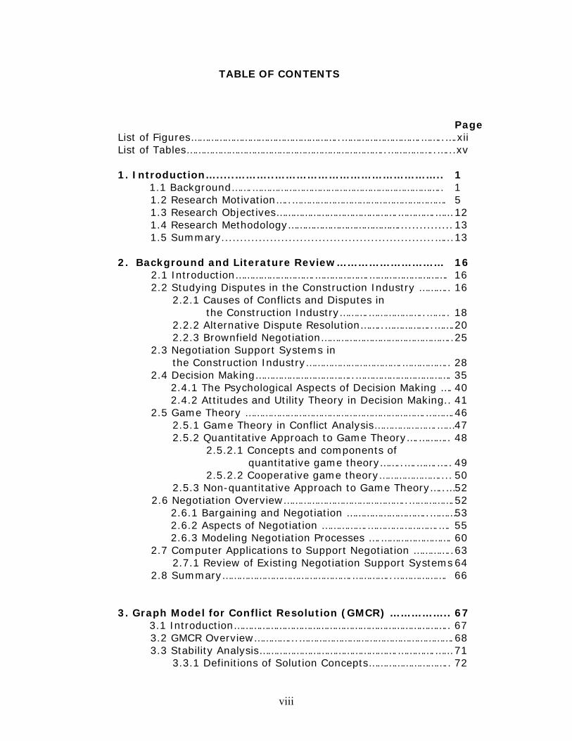
TABLE OF CONTENTS
Page List of Figures……………………………………………..……………………….……..….xii List of Tables……………………………………………………………..……………..…...xv 1. Introduction….....………..……………………………………….. 1 1.1 Background…….………………………………………………………….. 1 1.2 Research Motivation…..………………………………………………. 5 1.3 Research Objectives…………………………………….………….…… 12 1.4 Research Methodology…………………………………............... 13 1.5 Summary.........................................................…... 13 2. Background and Literature Review………………………… 16
2.1 Introduction……………………….……………….………………………. 16 2.2 Studying Disputes in the Construction Industry ……….. 16
2.2.1 Causes of Conflicts and Disputes in the Construction Industry……….………………..…….. 18
2.2.2 Alternative Dispute Resolution……..……………..……. 20 2.2.3 Brownfield Negotiation……………………………………….. 25
2.3 Negotiation Support Systems in the Construction Industry…………………………….…………….. 28
2.4 Decision Making……………………………..……………………………. 35 2.4.1 The Psychological Aspects of Decision Making …. 40 2.4.2 Attitudes and Utility Theory in Decision Making.. 41
2.5 Game Theory ……………………………………………………….………. 46 2.5.1 Game Theory in Conflict Analysis………………….…… 47 2.5.2 Quantitative Approach to Game Theory….……….. 48
2.5.2.1 Concepts and components of quantitative game theory……..….…….….. 49
2.5.2.2 Cooperative game theory………………….... 50 2.5.3 Non-quantitative Approach to Game Theory…..… 52
2.6 Negotiation Overview……………………………………..……………. 52 2.6.1 Bargaining and Negotiation ………………………..………53 2.6.2 Aspects of Negotiation …………….…………………….…. 55 2.6.3 Modeling Negotiation Processes ….……………………. 60
2.7 Computer Applications to Support Negotiation ………….. 63 2.7.1 Review of Existing Negotiation Support Systems 64
2.8 Summary……………………………………….…………..………………. 66 3. Graph Model for Conflict Resolution (GMCR) …………….. 67 3.1 Introduction………………………………………………………………….. 67 3.2 GMCR Overview…………...………………………………………………. 68 3.3 Stability Analysis………………………………………….………….…… 71
3.3.1 Definitions of Solution Concepts……………………….. 72
ix
3.4 Sensitivity Analyses……………………………………............... 74 3.5 Summary.........................................................…... 75 4. Attitude-Based Strategic Negotiation Methodology
Involving Two Decision Makers……………………….…….. 76 4.1 Introduction……………………………………………………….……….. 76 4.2 Propose Negotiation Framework ……………….……………….. 77 4.3 Understand Construction Negotiations ……..……….……… 77
4.3.1 General Negotiation Characteristics…………………… 79 4.3.2 Negotiators’ Characteristics……………………….………. 81 4.3.3 Challenges and Needs………………………….……………. 81
4.4 Attitude-Based GMCR…………………………….…..……..…..….. 84 4.4.1 GMCR Formal Definition…..……………………….……….. 84 4.4.2 Attitude Representation …………………………………….. 85 4.4.3 Formal Definition of Attitude…………………………….. 87 4.4.4 Attitude-Based Solution Concepts ……..…………….. 88 4.4.5 Propositions on Relationships among Attitude-Based Stability Types……….……………….. 94
4.5 Strategic Negotiation Methodology: A Brownfield Case Study……………………………………………………..…………………….. 95
4.5.1 Feasible States and Preferences ……………………….. 97 4.5.2 Reachable List…………………………….…………………….. 99 4.5.3 Stability Analysis…………………………………………….…… 100 4.5.4 Analysis of DMs’ Neutral Attitudes
towards Each Other………………………………………….. 101 4.5.4.1 Assessment of the stability…..………….... 102
4.5.5 Analysis of DMs’ Negative Attitudes towards Each Other………………………………………….. 104 4.5.5.1 Assessment of the stability…..………….... 106
4.5.6 Analysis of DMs’ Positive Attitudes towards Each Other…………………………………..……… 107 4.5.6.1 Assessment of the stability…..………….... 109
4.6 Discussion of the Resulting Strategic Decisions …….….. 110 4.6.1 Attitude Case 1 ………………………………………………….. 113 4.6.2 Attitude Case 2 ………………………………………………….. 114 4.6.3 Attitude Case 3 ………………………………………………….. 115
4.7 Summary……………………..………………………………………….….. 117
5. Attitude-based Strategic Negotiation Methodology Involving Multiple Decision Makers………………………….. 119
5.1 Introduction……………………………………………………….….…….. 119 5.2 Real-Life Brownfield Case Study ……….……………..……….. 119
5.2.1 The Causes of the Conflict…….…….……….…………… 122 5.3 Identifying the DMs and Their Options …..………..…..….. 123 5.4 Infeasible States ……………………………………….…………….….. 125 5.5 DMs’ State Rankings…….………………………………………….….. 126 5.6 Stability Analysis…….……………………………………………….….. 128
5.6.1 Reachable List……………….…………………………..……… 128

x
5.6.2 Attitude-Based Stability Analysis for Three DMs. 130 5.6.3 Proposed Algorithms for Removing Infeasible Attitude Cases..………………………….…… 132
5.6.4 Determining the Most Relevant Feasible Attitude Cases ……………………………….………………… 135 5.6.5 Analysis of the Most Relevant Attitude Cases…….137
5.7 Discussions of the Results of the Stability Analyses ….. 142 5.7.1 Qualitative Analysis of the Findings …..………..…… 143 5.7.2 Quantitative Analysis of the Findings………………... 149
5.7.2.1 Step 1: Determine the attitude values.. 150 5.7.2.2 Step 2: Determine the average satisfaction values………………... 151 5.7.2.3 Step 3: Draw attitude-satisfaction graph155
5.7.3 Determining the Most Beneficial Strategic Decision………………………………………………………………. 160 5.7.3.1 Updated level of information for the case study ………..………………………... 165
5.8 Evolution of the Brownfield Conflict…………………………..… 166 5.9 Summary …………………….………………………………………….….. 168
6. Attitude-Based Tactical Negotiation Involving Two Decision Makers……………………………………….………….. 171
6.1 Introduction……………………………………………………….……….. 171 6.2 Tactical Negotiation Methodology: A Brownfield Case Study ……………………………..………….. 172
6.2.1 Step 1: Identify Conflicting Issues within the Strategic Decision ……………………………………… 173 6.2.2 Step 2: Determine the DMs’ Utility Functions...… 173 6.2.3 Step 3: Obtain an Integrated Utility Function for Each Issue……………………………………………..…….. 180 6.2.4. Step 4: Select the Best Decision Value …………… 185
6.3 Sensitivity to the DMs’ Attitudes………………………..…..….. 187 6.4 Discussion of the Results ……………………………………….….. 192 6.5 Summary……………………..………………………………………….….. 195
7. Attitude-Based Tactical Negotiation Involving Multiple Decision Makers……………………………………….………….. 196
7.1 Introduction……………………………………………………….……….. 196 7.2 Generalized Tactical Negotiation Methodology..……….. 196 7.3 Tactical Negotiation Process: Multiple DMs and Issues 198
7.3.1 Approach 1: One Issue at a Time.………………..…… 200 7.3.2 Approach 2: Two DMs at a Time …………………..… 203
7.4 Application to the School of Pharmacy Tactical Negotiation …………………………………………………………….….. 205
7.4.1 Step 1: Decompose Negotiation Issues into Sub-Issues …………………………………………...…… 206 7.4.2 Step 2: Identify the DMs’ Least Expectations … 209 7.4.3 Step 3: Simulate the Tactical Negotiation …….… 210
xi
7.4.4 Step 3a: Tactical Negotiations between PolyOne and the City ….……………………………………..211 7.4.5 Step 3b: Tactical Negotiations between PolyOne and UW………………………………………….....… 214 7.4.6 Step 3c: Tactical Negotiations between the City and UW ……………………………………….....… 215 7.4.7 Discussion of the Tactical Negotiation Results … 217
7.5 Attitude-Based Sensitivity Analysis ……………………….….. 224 7.5.1 Discussion of Attitude-Based Sensitivity Results 229 7.5.2 Monte Carlo Simulation ……………………………...…… 232
7.6 Case Study Updates …………………….………………….…….….. 239 7.7 Lessons Learned …………………….……………………………….….. 241 7.8 Summary ……………………………….……………………………….….. 244
8. Decision Support System for Construction Negotiation. 246
8.1 Introduction……………………………..……………………….……….. 246 8.2 Design of the Proposed System……………………………….…. 246
8.3 Prototype Negotiation Decision Support System ………. 247 8.3.1 Step 1: Determine the DMs and Their Options … 250 8.3.2 Step 2: Rank DMs’ States …………………………...…… 251 8.3.3 Step 3: Specify DMs’ Reachable Lists………………. 253 8.3.4 Step 4: Perform the Attitude-Based Stability Analysis……………………………………………………………... 254 8.3.5 Step 5: Select a Strategic Decision ……….…...…… 257
8.4 Tactical Negotiation Support………………..…………….……….. 258 8.5 Summary……………………………..……………………….…….……….. 261 9. Conclusions………………………………………..…….………….. 263
9.1 Introduction……………………………..………………………..……….. 263 9.2 Research Summary………………………………………………………. 263 9.3 Research Contributions……………..…………………………………. 268
9.4 Recommendations for Future Research………………………. 271 References………………………………………………………………… 274
Appendix A …………………………….………………………………… 287
xii
LIST OF FIGURES
Tile Caption Page _______________________________________________________________
Figure 1.1 Worldwide Litigation Fees for Various Industries 1 Figure 1.2 ADR Methods in Construction 4 Figure 1.3 Proposed Research Methodology 14
Figure 2.1 Key Considerations in a Contracting Strategy 18 Figure 2.2 Dispute Resolution Continuum 24 Figure 2.3 Engineering Decision Making 37 Figure 2.4 Perspectives on Decision Making 38 Figure 2.5 Exponential Utility Functions 45 Figure 2.6 Genealogy of Formal Conflict Models 48 Figure 2.7 Aspects of Negotiation Analysis 55 Figure 2.8 Negotiation Process Flowchart 63
Figure 3.1 Systematic Procedure for Applying GMRC 69 Figure 4.1 Proposed Negotiation Framework 78 Figure 4.2 GMCR Procedures Using Rational and Attitude-Based Analyses 93 Figure 4.3 Integrated Graph Model and State Preference for DMs 99 Figure 4.4 Stability Analysis Tableau for Two DMs with Rational Attitudes 102 Figure 4.5 Attitude-Based Stability Analysis Tableau for Two DMs with Negative Attitudes 105 Figure 4.6 Attitude-Based Stability Analysis Tableau for Two DMs with Positive Attitudes 108 Figure 4.7 Three Sets of Equilibria for Three Attitude Cases 113 Figure 5.1 Satellite Image of the Former Brownfield Site 120 Figure 5.2 Graph Model for the DMs Involved in the School of Pharmacy Negotiations 131 Figure 5.3 Eight Strategic Orientations of DMs’ Negotiations 133 Figure 5.4 Stability Tableau for Case 1 139 Figure 5.5 Stability Tableau for Case 2 139 Figure 5.6 Stability Tableau for Case 3 140 Figure 5.7 Stability Tableau for Case 4 140 Figure 5.8 Stability Tableau for Case 5 141

xiii
Figure 5.9 Stability Tableau for Case 6 141 Figure 5.10 The Results of the Stability Analysis for the Six Attitude Cases 142 Figure 5.11 The Proposed Framework for the Quantitative Analysis 150 Figure 5.12 Combined Satisfaction Level of the Equilibrium States Disregarding the Influence of DMs’ Attitudes 154 Figure 5.13 Sorted Satisfaction Level of the Equilibrium States Disregarding the Influence of DMs’ Attitudes 154 Figure 5.14 Attitude-Satisfaction Graph for Attitude Case 6 156 Figure 5.15 The Attitude Satisfaction Relationship for Attitude Cases 1, 2, 4, and 5 158 Figure 5.16 Attitude Satisfaction Relationship for Attitude Cases 3 and 6 158 Figure 5.17 Satisfaction and Attitude Values for the Six Attitude Cases 162 Figure 5.18 Overall Preference Sorted for the Resulting Equilibrium States 164 Figure 6.1 Changes in Utility Value with Changes in Function Form 178 Figure 6.2 The DMs’ Utility Functions for the “Price” Issue 180 Figure 6.3 The Process of Integrating Utility Function Forms 181 Figure 6.4 Tactical Negotiation Process Involving Two DMs 183 Figure 6.5 Decision with the Maximum Utility Value 186 Figure 6.6 The Sensitivity of the DMs’ Attitudes to Negotiation Results 189
Figure 7.1 Pair-wise Negotiation Used to Formulate Generalized Tactical
Negotiation Methodology 197 Figure 7.2 Two Approaches for Conducting Tactical Negotiation 200 Figure 7.3 The Hierarchy of Negotiation Issues for the School of Pharmacy Negotiations
207 Figure 7.4 Simulation of the Tactical Negotiations for the School of Pharmacy 211 Figure 7.5 Tactical Negotiations between PolyOne and the City 213 Figure 7.6 Tactical Negotiations between PolyOne and UW 215 Figure 7.7 Tactical Negotiations between the City and UW 216 Figure 7.8 Sensitivity Analysis for a Specific DM in PolyOne – City Negotiations 226 Figure 7.9 Sensitivity Analysis for a Specific DM in PolyOne – UW Negotiations 227 Figure 7.10 Sensitivity Analysis for a Specific DM in City – UW Negotiations 228 Figure 7.11 Overall Results of the Sensitivity Analysis for the Tactical Negotiations for the School of Pharmacy 230 Figure 7.12 The Application of Monte Carlo Simulation for the Case Study233 Figure 7.13 Histograms for PO – City Resulting from the Monte Carlo
xiv
Simulation 235 Figure 7.14 Histograms for PO – UW Resulting from the Monte Carlo Simulation 236 Figure 7.15 Histograms for City – UW Resulting from the Monte Carlo Simulation 237 Figure 7.16 The UW School of Pharmacy under Construction 242 Figure 8.1 The NDSS Main Menu Screen 248 Figure 8.2 Components of the Proposed NDSS 249 Figure 8.3 Decision Makers Screen in the Proposed NDSS 251 Figure 8.4 The DMs’ State Rankings Screen in the Proposed NDSS 252 Figure 8.5 Reachable Lists Screen in the Proposed NST 254 Figure 8.6 Automated Attitude-Based Stability Analysis Using the Proposed NDSS 255 Figure 8.7 “Strategic Decision” Screen in the Proposed NDSS 257 Figure 8.8 Tactical Negotiation Screen in the Proposed NDSS 259
xv
LIST OF TABLES
Title Caption Page ________________________________________________________________
Table 2.1 Compiled Causes of Disputes in the Construction Industry 19 Table 2.2 The Characteristics of ADR Techniques 22 Table 2.3 The Objectives of Brownfield Reconstruction 26 Table 2.4 Reviewed Literature of Negotiation Support Systems in the Construction Industry 30
Table 2.5 Major Psychological Aspects of Decision Making 42 Table 2.6 Game Theory Classification 49 Table 2.7 Characteristics of Behavioral Negotiation 59 Table 2.8 A Summary of Literature about Negotiation Support Systems 65 Table 3.1 Solution Concepts Implemented in GMCR 72 Table 4.1 Negotiators’ Characteristics in Brownfield Reconstruction 83 Table 4.2 Assumptions on Relationships between Attitudes and Behaviors 86 Table 4.3 Tabular Representation of Attitudes 88 Table 4.4 Attitudes of DMs ‘o’ and ‘g’ in a Regular Analysis 88 Table 4.5 Rational and Attitude-Based Solution Concepts in GMCR 92 Table 4.6 Feasible States for the Case Study 98 Table 4.7 Reachable Lists for the Case Study 100 Table 4.8 Summary of the Stability Analysis for the Case Study 111 Table 4.9 Results for the Owner 112 Table 4.10 Results for the Government 112 Table 5.1 The DMs and Their Options in the UW School of Pharmacy Negotiations 124 Table 5.2 Infeasible States for the Case Study 125 Table 5.3 Resulting Feasible States for the Case Study 126 Table 5.4 DMs’ State Rankings for the School of Pharmacy Negotiations 127 Table 5.5 Reachable Lists for the School of Pharmacy Negotiation 129 Table 5.6 Algorithm for Removing Infeasible Attitude Cases in Negotiations with Two DMs 134 Table 5.7 Algorithm for Removing Infeasible Attitude Cases in

xvi
Negotiations with Three DMs 134 Table 5.8 Algorithm for Removing Infeasible Attitude Cases in Negotiations with n DMs 136 Table 5.9 The Most Relevant Attitude Cases for the School of Pharmacy Negotiations 138 Table 5.10 Attitude Values for Attitude Case 6 151 Table 5.11 Satisfaction Values for States in the DMs’ State Rankings 152 Table 5.12 The Average Satisfaction Values for Equilibrium States 6 and 8 153 Table 5.13 Attitude and Satisfaction Values for Six Attitude Cases 157 Table 5.14 Values of the DM’s Attitude and Satisfaction 161 Table 5.15 Combined DMs’ Satisfaction and Attitude Values for Attitude Case 6 163 Table 5.16 Overall Preference for the Equilibrium States 164 Table 5.17 State Transition for the Brownfield Conflict 166 Table 6.1 The Results of the Sensitivity of the DMs’ Attitudes 192 Table 7.1 Tactical Issues Identified within the Strategic Decision 206 Table 7.2 The Tactical Negotiation Results for the School of Pharmacy 218 Table 7.3 DMs’ Shares of the Costs of the Tactical Issues 222 Table 7.4 Summary of the Monte Carlo Simulation Results for the Case Study 238
1
CHAPTER 1: Introduction
1.1. Background
The construction industry is one of the largest industries in the world, with
members who are expert in planning, design, construction, operation, and
administration. Construction projects have become increasingly complex, with
the parties involved often having conflicting objectives. For example, the owner
would like a project to be inexpensive and quickly completed, while the contractor
wants large and income-generating projects with few time restrictions. According
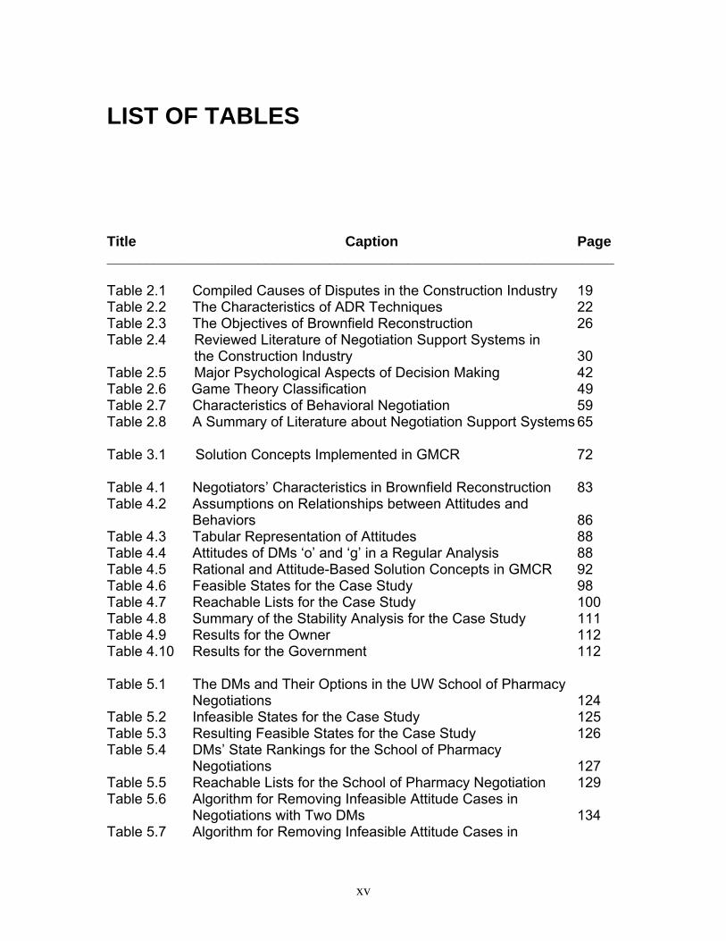
to Litigation Trends Survey Findings (LTSF, 2006), construction firms worldwide
spend close to 31 million US dollars annually on litigation: the second highest
expenditure by type of industry, as shown in Figure 1.1.
8.3
2.1
11.812.3
3133
9.77.4
0
5
10
15
20
25
30
35
Insu
ranc
eCo
nstru
ctio
nM
anuf
actu
ring
Ener
gyHe
alth
Car
eTe
chno
logy
Fina
ncia
l
Reta
il
Industry
US$M
illio
n
Litigation Fees
Figure 1.1: Worldwide Litigation Fees for Various Industries (LTSF, 2006)

2
In the highly competitive multi-party environment of construction, disputes can
arise for many reasons, such as the complexity and magnitude of the work, the
lack of coordination among the contracting parties, poorly prepared and/or
executed contract documents, inadequate planning, financial issues, and
disagreements about methods of solving on-the-spot site-related problems. Any
one of these factors can derail a project and lead to complicated litigation or
arbitration, increased costs, and a breakdown in the communication and
relationships between parties (Harmon, 2003).
According to the Department of Justice Canada (1995), construction is the
industry that has the highest number of disputes. Moreover, Kumaraswamy
(1997) has found that about 75% of construction contracts have been the subject
of some types of dispute which represents an enormous expenditure of time,
effort, and human resources. In other words, the construction industry has
become an adversarial culture prone to conflict and disputes (Brooker and
Lavers, 1997; Fenn et al., 1997; Garrett, 2002; Kellogg, 2001; Kumaraswamy,
1997; Mathews, 1997). The adversarial attitude prevalent in many disputes
undermines the cooperative environment necessary for the success of a project
and is at odds with the collaborative nature required in construction activities. A
great deal of research has been devoted to finding ways to reduce the number
and magnitude of these conflicts and more effective approaches are needed if
sustainable solutions are to be found for the current types of conflicts (Barnett,
1997).
3
The three major parties traditionally involved in a construction project are the
owner, the consultant, and the contractor. Clearly, the successful delivery of a
project requires their full cooperation and collaboration: time, costs, resources,
and objectives must be coordinated. However, differences in the perceptions of
the parties involved in a project make conflicts and disputes inevitable.
Therefore, resolving disputes has become an essential component of
construction administration and many studies have been conducted with respect
to finding effective dispute resolution methods (Barnett, 1997; Cheung et al.,
2002; Diekmann and Girard, 1995; Doug, 2006; Rameezdeen and Gunarathna,
2003; and Shen et al., 2007).
The traditional method of resolving construction disputes is litigation, which is
usually complicated because of unresolved conflicts or disputes connected with
large, complex projects (Pinnell, 1999). The enormous amounts of time and
money expended by all parties involved in litigation (Figure 1.1) have led to the
emergence of other dispute resolution methods, called Alternative Dispute
Resolution (ADR) tactics (Harmon, 2003). The main purpose of ADR tactics is to
resolve disputes with the ‘‘least possible intervention by an outside third party’’
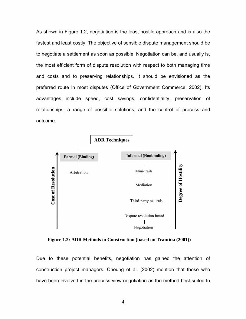
(Gillie et al., 1991). As illustrated in Figure 1.2, two groups of ADR tactics are
used in construction: formal-binding and informal-nonbinding tactics (Di-Donato,
1993). Formal-binding ADR is predominantly arbitration, while informal-
nonbinding ADR tactics include mini-trials, mediation, third-party neutrals, dispute
resolution boards, and negotiation (Trantina, 2001).
4
As shown in Figure 1.2, negotiation is the least hostile approach and is also the
fastest and least costly. The objective of sensible dispute management should be
to negotiate a settlement as soon as possible. Negotiation can be, and usually is,
the most efficient form of dispute resolution with respect to both managing time
and costs and to preserving relationships. It should be envisioned as the
preferred route in most disputes (Office of Government Commerce, 2002). Its
advantages include speed, cost savings, confidentiality, preservation of
relationships, a range of possible solutions, and the control of process and
outcome.
Due to these potential benefits, negotiation has gained the attention of
construction project managers. Cheung et al. (2002) mention that those who
have been involved in the process view negotiation as the method best suited to
ADR Techniques
Formal (Binding)
Arbitration
Informal (Nonbinding)
Third-party neutrals
Mediation
Mini-trails
Negotiation
Cos
t of R
esol
utio
n
Deg
ree
of H
ostil
ity
Dispute resolution board
Figure 1.2: ADR Methods in Construction (based on Trantina (2001))

5
preserving or enhancing existing job relationships. Their research also points out
that negotiation is effective in reducing costs and opening channels of
communication. In addition, according to an official document published by the
Office of Government Commerce (OGC) (2002), negotiation is by far the most
common form of dispute resolution, with a variety of related systems having been
developed for employing it. Despite the importance of negotiation and the
availability of formal negotiation techniques, they have not thus far been widely
used in the construction industry.
1.2. Research Motivation
The goal of this research is to develop a systematic negotiation methodology,
especially suited for complex construction disputes, which incorporates the
negotiators’ attitudes not only at the strategic level of decision making but also at
the tactical (detailed) level of decision making. The research has been motivated
by the following considerations.
A) Negotiation is important to the construction industry: Most construction
projects involve cost overruns, time extensions, and conflicts among parties. The
widespread extent of these problems is generally attributed to two main factors
(Hegazy, 2002): the unique and highly uncertain nature of construction projects
and the fragmented and highly competitive nature of the construction industry. In
this challenging environment, any of the variables that affect a project, such as
the weather, the interpretation of the contract, soil conditions, labor, or

6
equipment, can become a problem at any moment. Because each party then
strives not to take the blame for the consequences of any difficulties that arise,
disputes and conflicts are inevitable. Efficient conflict and dispute management
techniques, such as negotiation, thus become key to the success of projects and
of the parties involved in the project. It should be mentioned that construction
negotiations take place among the parties who are often bounded by a contract.
However, there are negotiations among construction parties who are not
necessarily bounded by a contract.
B) The construction industry lacks negotiation support: Negotiation is
potentially one of the most effective methods of ADR in the construction industry.
It provides a process whereby construction disputants can communicate to one
another their conflicting interests and resolve differences so that further disputes
arising from misperceptions of the current conflict can be prevented. The ability
of construction managers to effectively negotiate significantly influences the
performance of the project.
In spite of the importance of negotiation, with respect to construction, it has been
the subject of little research or education (Dudziak and Hendrickson, 1988).
Engineering managers, for example, learn negotiating skills mainly through
experience and observation (Smith, 1992). Moreover, negotiation in construction
can be difficult since the individuals charged with negotiating the settlement are
reluctant to make concessions because of the risk of having to explain them to
7
uninformed senior management. In other words, construction disputants lack
organized negotiation support to help them handle complex construction conflicts
and disputes. Developing negotiation support tools that can provide assistance
for construction managers and administrators is therefore important.
In response to the need for negotiation support tools, several studies have been
conducted in the area of negotiation support systems (NSS) (Cheung et al.,
2004; Li, 1996; Molenaar et al., 2000; Omoto et al., 2002; Ren et al., 2003; and
Yaoyueyong et al., 2005). Such systems, however, seem to suffer from the
following restrictions:
• They do not consider the psychological aspects of the decision makers in
the negotiation and thus fail to address attitude, which is one of most
influential psychological factors in negotiation (Kahneman and Tversky,
2000).
• They are restricted to informing decision makers about the progress of
only the current negotiation and cannot provide details about past rounds
of negotiation, or about the parties involved, or their preferences.
• They do not consider the characteristics of disputes and disputants in the
negotiation methodology.
• They fail to implement suitable negotiation strategies that incorporate
changes, since they do not take into account the effect of moves and
countermoves by decision makers during interactive strategic decision
making.
8
• They provide decision makers with only cardinal payoff values for
conflicting issues and do not suggest to the involved parties any strategic
equilibrium state.
• They lack a systematic approach for complementing varying levels of
negotiation, such as complementing strategic and tactical levels of
decision making to develop a comprehensive negotiation methodology.
Therefore, if current negotiation methodologies are to overcome the above
limitations and constraints, they need improvement.
C) The psychological aspects of negotiation need to be considered:
Negotiation is considered a decision-making process in which decision makers
take into account the social factors (e.g., economic, psychological, financial, and
political) that affect their offers and counteroffers during negotiation. Depending
on the circumstances surrounding the decision, some of these aspects are more
important than others. Psychological factors, such as attitude, often have
significant influence on the outcome of the negotiation. For example, when two
parties who have negative attitudes toward each other negotiate, the outcome of
the negotiation is unlikely to be productive. The attitudes of decision makers
toward one another may also change during each round of negotiation. For
example, two decision makers may initially have negative attitudes toward each
other, but as negotiation continues and they share their concerns and limitations,
they may develop more positive attitudes and eventually reach a productive
9
outcome. Therefore, using a negotiation methodology that considers the attitudes
of the negotiators is more likely to provide a reliable outcome that can be a stable
solution to the conflict.
When parameters are set for conflict situations, the few negotiation models
prepared for the construction industry (Cheung et al., 2004; Molenaar et al.,
2000; and Omoto et al., 2002) lack consideration of the psychological states of
the decision makers. A key goal of this research is therefore to incorporate the
attitudes of the decision makers into the modeling of the negotiation process so
that more realistic and reliable equilibrium outcomes can be suggested. In other
words, a comprehensive negotiation methodology should be capable of including
the psychological aspects of negotiation, such as the negotiators’ behavior and
attitudes, at both the strategic and the tactical levels of the decision making
process. Such unified methodology can then suggest the most stable solution.
D) Decision analysis tools should be integrated within the negotiation
methodology: Recent research in negotiation has shown the advantage of
employing decision-making tools to help produce better negotiation outcomes
(Bellucci and Zeleznikow, 1998; Kersten, 2002; Matwin et al., 1989; and
Thiessen and McMahon, 2000). Such integration provides the following
advantages:
• Effective communication among decision makers,
• The capability of learning from experience,
10
• Explanations helpful to decision makers,
• The modelling of the dynamic properties of the negotiation, and
• The ability to draw reasonable conclusions and clear strategic guidance.
Negotiation Decision Support Systems (NDSSs) have been used successfully in
other domains, such as family counseling (Bellucci and Zeleznikow, 1998); E-
commerce and E-negotiations (Kersten, 2002); and manufacturing disputes
(Sycara, 1993). In spite of the potential benefits and inherent capabilities of
NDSSs, the construction industry has not been sufficiently introduced to these
recent developments in negotiation methodologies and support systems. For
example, the Graph Model for Conflict Resolution (GMCR) methodology was
developed by Fang et al. (1993); the concept of utility theory was explained by
Fishrburn (1970); the concept of Efficiency Frontier was introduced by Raiffa et
al. (2002); and the concepts of Even Swaps and Value-Focused Thinking were
introduced by Hammond et al. (1999) and Keeney (1992), respectively. These
concepts have not been widely employed for addressing construction disputes.
Moreover, such theories and methodologies have potentially beneficial
applications in resolving construction conflicts because they can model the risk
attitudes and behaviors of decision makers, and can effectively account for
negotiation-related uncertainties.
E) Challenges in brownfield negotiations need to be overcome: As an area
of construction in which negotiation can be applied, this research focuses on
11
brownfield negotiations: a growing problem in the Canadian construction industry
and elsewhere (De Sousa, 2001 and Ellerbusch, 2006). A brownfield is
contaminated land that lies unused and unproductive. Due to the enormous
amount of uncertainty and the number of unexpected events involved in
brownfield redevelopment, the parties involved (e.g., the current owner and the
government) spend tremendous amounts of time in multiple rounds of negotiation
in the hope of reaching an agreement about cleaning up the contaminated site
(De Sousa, 2000). They must analyze past and current information in order to
make effective offers and counteroffers that can lead to an agreement about the
transfer of ownership and the decontamination and redevelopment of a
brownfield property. The negotiating parties may, however, lack negotiation skills
and be unable to handle the negotiation process efficiently, communicate their
concerns and preferences, and make suitable decisions about the problem.
Although the parties involved are willing to reach a mutual agreement
cooperatively, the negotiation process in brownfield projects is complex and often
unproductive, particularly when few practical solutions are suggested by any of
the parties (Begley, 1997).
A negotiation support system that provides more effective practical guidelines for
the parties involved is therefore needed (Hipel et al., 2009). Such brownfield
negotiation tools must take into consideration the risk attitudes and behavioral
characteristics of the current owner, the government, the stakeholders involved,
and possibly the future purchaser.

12
1.3. Research Objectives
The primary objective of this research is to provide a better understanding of the
negotiation processes among the decision makers involved in construction
disputes. Accordingly, a systematic negotiation framework has been developed
that considers decision makers’ attitudes in order to help the negotiating parties
reach a stable mutual agreement. The proposed negotiation methodology
provides the parties involved with both strategic decision options and tactical
(detailed) payoff outcomes. The specific objectives are as follows:
1. To understand how construction negotiators behave and negotiate in
practice to reach mutual compromises with respect to conflicting issues;
2. To identify, with respect to construction, the characteristics of both
negotiations (e.g., the parties involved, the type and number of conflicting
issues, and the type of project) and negotiators (e.g., position, choices);
3. To study the applications of game theory, negotiation analysis, the Graph
Model analysis, utility theory to model a construction negotiation process;
4. To develop an attitude-based negotiation methodology at both the
strategic and tactical levels of negotiation for addressing and resolving
construction disputes when multiple decision makers and multiple
conflicting issues are involved;
5. To demonstrate the application of the proposed negotiation methodology
in real-life brownfield case studies; and
6. To implement the proposed negotiation methodology into a construction
negotiation decision support system.
13
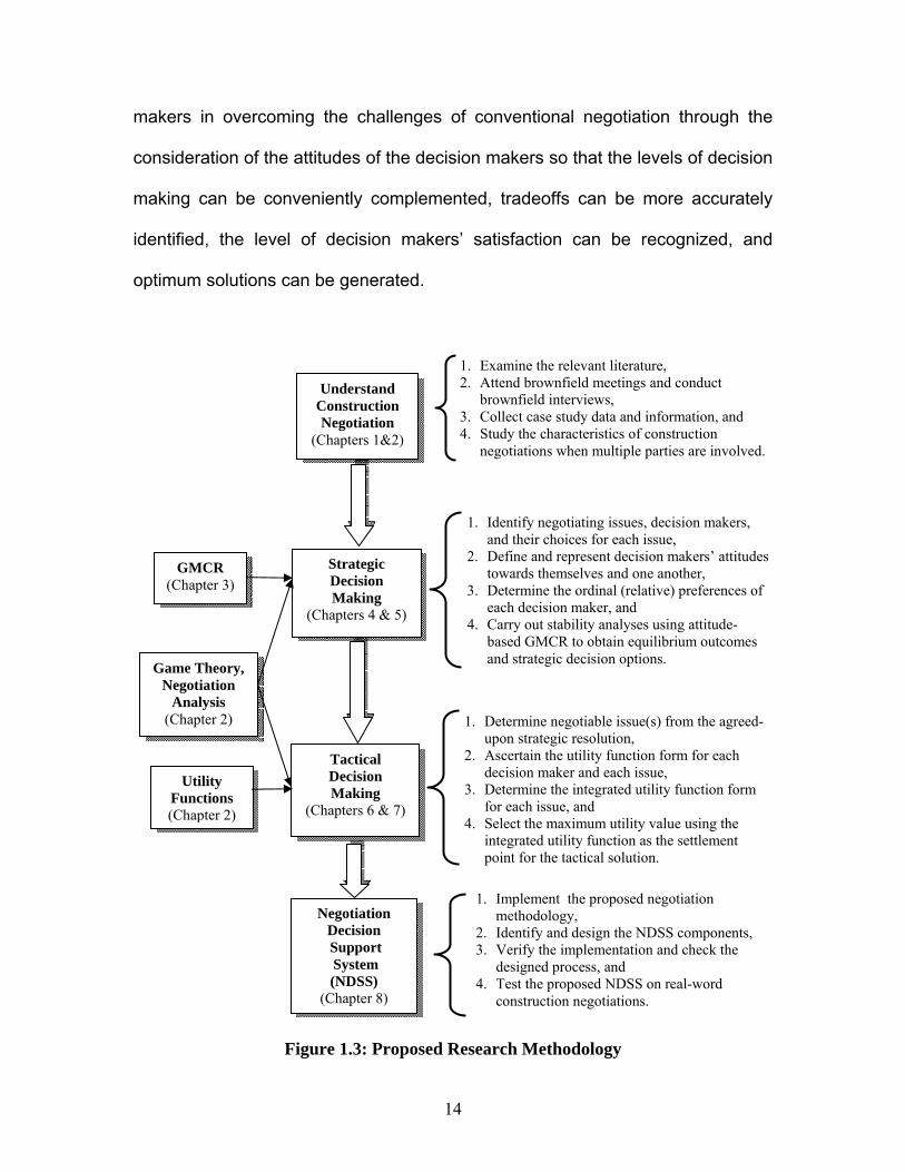
1.4. Research Methodology
To achieve the above objectives, relevant theories, techniques, and approaches
in the literature have been reviewed and appropriately refined and expanded in
order to arrive at a novel decision-making methodology for engineering purposes
particularly suited to construction decision making (Yousefi et al., 2008). The
proposed methodology will systematically incorporate the attitudes of the
negotiators into the modeling of the negotiation at the level of strategic decision
analysis as well as at the tactical level. The systematic research methodology is
depicted in Figure 1.3.
1.5. Summary
The goal of this research is to develop an innovative negotiation methodology
that takes into account the attitudes of decision makers at two levels of decision
making: strategic and tactical. At the strategic level, the Graph Model for Conflict
Resolution is systematically employed as a means of determining a potential
overall agreement, or set of resolutions, that is possible given the competing
interests of the decision makers involved in the negotiation process. At the
tactical level, the new methodology allows a possible strategic solution to be
studied in depth using utility functions to determine the detailed trade-offs or
concessions needed for the parties to reach a mutually acceptable solution.
This research may help participants facilitate or mediate the negotiation of
disputes in construction projects. The proposed methodology may assist decision
14
makers in overcoming the challenges of conventional negotiation through the
consideration of the attitudes of the decision makers so that the levels of decision
making can be conveniently complemented, tradeoffs can be more accurately
identified, the level of decision makers’ satisfaction can be recognized, and
optimum solutions can be generated.
Figure 1.3: Proposed Research Methodology
Negotiation Decision Support System (NDSS)
(Chapter 8)
Game Theory, Negotiation
Analysis (Chapter 2)
1. Examine the relevant literature, 2. Attend brownfield meetings and conduct
brownfield interviews, 3. Collect case study data and information, and 4. Study the characteristics of construction
negotiations when multiple parties are involved.
GMCR (Chapter 3)
Strategic Decision Making
(Chapters 4 & 5)
Understand Construction Negotiation
(Chapters 1&2)
Utility Functions (Chapter 2)
Tactical Decision Making
(Chapters 6 & 7)
1. Identify negotiating issues, decision makers, and their choices for each issue,
2. Define and represent decision makers’ attitudes towards themselves and one another,
3. Determine the ordinal (relative) preferences of each decision maker, and
4. Carry out stability analyses using attitude-based GMCR to obtain equilibrium outcomes and strategic decision options.
1. Determine negotiable issue(s) from the agreed-upon strategic resolution,
2. Ascertain the utility function form for each decision maker and each issue,
3. Determine the integrated utility function form for each issue, and
4. Select the maximum utility value using the integrated utility function as the settlement point for the tactical solution.
1. Implement the proposed negotiation methodology,
2. Identify and design the NDSS components, 3. Verify the implementation and check the
designed process, and 4. Test the proposed NDSS on real-word
construction negotiations.
15
This chapter has emphasized the need for using negotiation tactic in construction
due to their lower cost and less hostile attributes compared with other ADR
tactics, such as litigation and arbitration. The motivation for this research has
been briefly explained. The objectives of the research have been listed and the
proposed research methodology outlined. Chapter 2 provides a comprehensive
review of literatures related to conflicts, disputes, negotiation, and decision-
making, with respect to the construction industry, followed by Chapter 3, which
briefly introduces the Graph Model for Conflict Resolution (GMCR). The
development of the new negotiation methodology at the strategic level for both
two and multiple decision makers is discussed in Chapters 4 and 5, respectively.
The negotiation methodology at the tactical level, again for both two and multiple
decision makers, is presented in Chapters 6 and 7, respectively. The
implementation of the proposed methodology in the design of a construction
negotiation decision support system is explained in Chapter 8, and Chapter 9
contains concluding remarks, research contributions, and suggestions for future
work.
16
CHAPTER 2 Background and Literature Review
2.1. Introduction
An overview of conflict and negotiation in construction projects is provided in this
chapter along with concepts, techniques, and methodologies related to decision
making that can be used to develop a negotiation methodology for complex
construction disputes. The fundamentals of decision making, particularly strategic
and tactical decision making, game theory, and negotiation analysis are
introduced. The relationship between game theory and negotiation analysis is
also explained and approaches used in modeling the negotiation process are
reviewed. Finally, computer applications that support negotiation, particularly in
the construction domain, are explained and the relevant literature is reviewed
and summarized.
2.2. Studying Disputes in the Construction Industry
The construction of a project is an integrated process. Every construction project
requires detailed planning and involves parties such as the owner, contractor,
and subcontractors, who are contractually integrated but who have different
responsibilities and knowledge. In such an environment, conflicts and disputes
can arise for many reasons, including the complexity and magnitude of the work,
lack of coordination among the contracting parties, poorly prepared and/or
17
executed contract documents, inadequate planning, financial issues, and
disagreements about solving many of the on-the-spot site-related problems. Any
one of these factors can derail a project and lead to complicated litigation or
arbitration, increased costs, and a breakdown in the parties’ communication and
relationship (Harmon, 2003). While changes in the work on construction projects
are not unusual, the manner in which these alternatives are addressed; or not,
can potentially affect the successful completion of a project by creating additional
unresolved and unproductive conflicts. If the construction conflicts are not
adequately addressed and managed, they can evolve into serious disputes
among the parties involved and, therefore, not only could the working
environment be damaged, but the cost and duration of projects may also be
significantly increased (Hartman and Jergeas, 1995).
The parties involved in the construction industry are usually bound contractually
and thus, the contract is the essential document used in the submission and
evaluation of claims. In the early stages of a project, the owner decides on a
contract strategy which takes into account the following aspects, as shown in
Figure 2.1 (Hegazy, 2002):
• The project objectives and constraints,
• A proper project delivery method,
• A reasonable design/construction interaction scheme,
• A proper contract form/type, and
• Administration practices.

18
Different considerations of these factors produce different contractual forms,
which shape the process by which conflicts are addressed in construction
projects.
Figure 2.1: Key Considerations in a Contracting Strategy (Hegazy, 2002)
2.2.1. Causes of Conflicts and Disputes in the Construction Industry
Although each construction project is unique, the causes of conflicts are
generally similar. They arise from the complexity and magnitude of the work,
from multiple parties having different objectives, from unrealistic expectations,
from poorly prepared and/or executed contract documents, from financial issues,
and from communication problems. A list of the identified causes of disputes in
construction is shown in Table 2.1; it represents a compilation from many studies
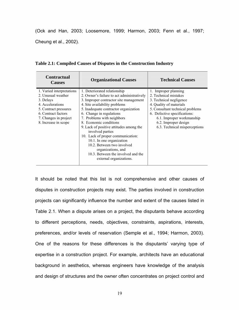
19
(Ock and Han, 2003; Loosemore, 1999; Harmon, 2003; Fenn et al., 1997;
Cheung et al., 2002).
Table 2.1: Compiled Causes of Disputes in the Construction Industry
Contractual Causes
Organizational Causes
Technical Causes
1. Varied interpretations 2. Unusual weather 3. Delays 4. Accelerations 5. Contract pressures 6. Contract factors 7. Changes in project 8. Increase in scope
1. Deteriorated relationship 2. Owner’s failure to act administratively 3. Improper contractor site management 4. Site availability problems 5. Inadequate contractor organization 6. Change in regulations 7. Problems with neighbors 8. Economic conditions 9. Lack of positive attitudes among the
involved parties 10. Lack of proper communication: 10.1. In one organization
10.2. Between two involved organizations, and
10.3. Between the involved and the external organizations.
1. Improper planning 2. Technical mistakes 3. Technical negligence 4. Quality of materials 5. Consultant technical problems 6. Defective specifications:
6.1. Improper workmanship 6.2. Improper design 6.3. Technical misperceptions
It should be noted that this list is not comprehensive and other causes of
disputes in construction projects may exist. The parties involved in construction
projects can significantly influence the number and extent of the causes listed in
Table 2.1. When a dispute arises on a project, the disputants behave according
to different perceptions, needs, objectives, constraints, aspirations, interests,
preferences, and/or levels of reservation (Semple et al., 1994; Harmon, 2003).
One of the reasons for these differences is the disputants’ varying type of
expertise in a construction project. For example, architects have an educational
background in aesthetics, whereas engineers have knowledge of the analysis
and design of structures and the owner often concentrates on project control and

20
administration. Conflicts and disputes arise when they have to communicate with
one another about the project because their background and training are very
different and lead to different perspectives on the project (Fenn et al., 1997).
None of the parties usually has an in-depth overall view, which may hamper the
finding of a common meeting ground.
Although conflicts are an inherent part of every construction project, it is very
important that conflict among parties be reduced. Therefore, any viable means of
reducing the incidence of conflicts and disputes (e.g., developing positive
attitudes among the parties involved) should have a positive effect on the
outcome of the project (Jergeas, 2008). The construction participants are
themselves aware that unresolved conflicts and their resulting legal and
consulting fees add no value to construction projects.
2.2.2. Alternative Dispute Resolution
Traditionally, unresolved conflicts and disputes involving large scales, complex
construction projects can be resulted in complex construction litigation (Pinnell,
1999). Litigation is a dispute when it has become the subject of a formal court
action or law suit. Anyone who has ever been involved litigation knows that it is
expensive, time consuming, emotionally draining and unpredictable. With
litigation, until a judge or jury decides who is right and who is wrong, the outcome
is not certain. Alternative Dispute Resolution (ADR) tactics, such as mediation,
has been gaining popularity as a method to remedy the shortcomings of litigation.
21
Lengthy and expensive litigation processes have made construction participants
less eager to have their day in court, opting instead to resolve their disputes
among themselves, as has been done for a long time (Glasner, 2000). In
response to the increased cost and duration of litigation, the construction industry
has gravitated toward ADR tactics (Mix, 1997; Treacy, 1995). Historically, the
construction industry has been seeking innovative and creative ways to resolve
conflicts and disputes arising from construction contracts (Henderson, 1996; Mix,
1997). Not only are the costs of court claims avoided, but there are also
intangible benefits to avoiding court cases such as maintaining reputation and
avoiding emotional stresses (Cheung et al., 2002). For example, arbitration and
mediation are similar in that they are alternatives to litigation, or are sometimes
used in conjunction with litigation to attempt to avoid litigating a dispute to its
conclusion. Both arbitration and mediation employ a neutral third party. Both can
be binding; however, it is customary to employ mediation as a non-binding
procedure and arbitration as a binding procedure. The characteristics of ADR
tactics are summarized in Table 2.2.
As shown in Figure 1.2, ADR techniques can include both binding (formal) and
nonbinding (informal) procedures (Kellogg, 2001; Honeyman et al., 2004).
Binding ADR is predominantly arbitration, and the binding method sometimes
used in construction (Di-Donato, 1993). Nonbinding ADR techniques normally
include mini-trials, mediation, third-party neutrals, Dispute Review Boards
(DRBs), and negotiation.

22
Table 2.2: The Characteristics of ADR Techniques (Harmon, 2003)
* Early Neutral Evaluation, **Dispute Review Board
Tactics
Application Advantages Drawbacks
Litigation
Traditional approach for large complex projects. Last preferred tactic.
Appropriate for large complex disputes, formal win-lose method with assigning damage compensations via a court appeal.
Expensive, time consuming, fraught with flaws, affect parties’ reputations.
Arbitration
Alternative to litigation with more preference, incorporated into standard contracts.
Very common usage, acceptance of evidences, maintains the confidentiality of the proceedings, more cost-efficient than litigation, preserved business relationship between parties.
More time preparation, no quick and easy answers to resolving the problem, procedural complexities, adversarial approach, lack of the appeal process.
Mediation
A nonbinding, consensual process, a form of distributive justice, a form of assisted or guided negotiation, better to use before arbitration.
Faster, less expensive, more confidential, and more satisfactory way than litigation, minimizing future disputes by maintaining open communication between the parties, creates a win-win outcome that satisfies both parties, very flexible.
Procedural complexities, leading to a compromise settlement, sometimes resulting in subjective outcomes which may confuse parties.
Med./Arb.
A hybrid of mediation and arbitration, binding mediation, considered as a new and enhances tactic.
Encourages the parties to settle rather than lose control of the outcome if arbitration becomes necessary, includes the capabilities of mediation and arbitration.
Creates some dilemmas for either pursue or hold back from mediation part, not so much used in the construction industry.
Mini-trial
A nonbinding hybrid ADR process, it is not a trial, and is held after other alternative dispute mechanisms have failed, but before an actual trial.
Predicts the results of an actual trial, thereby enabling the parties to come to a decision to resolve their dispute before applying for a full scale trial.
Presentations at a mini-trial are time limited, each party must have a relatively good understanding of its issues and the opposing parties’ refutations and issues.
ENE * (third-party
neutral)
Used early in the litigation process, a court-ordered process, an informal, nonbinding procedure.
Resolves disputes sooner rather than later, thereby circumventing the need for trial preparation, an alternative to expensive discovery and resolving complex technical issues.
Evaluation can be based on predicting the outcome of a trial or arbitration, the procedure is not very straightforward.
Partnering
Seeks to change attitudes about the relationships between parties, establishing trust and open communication, considers as a preventive dispute resolution.
Reduces exposure to litigation, cost overruns, and delays, promotes mutual rather than bifurcated goals, restores the spirit of cooperation.
Not a suitable tactic if the root causes of disputes are not addressed, needs a top-down approach, needs a huge amount of communication among parties.
DRB**
A unique, proactive, non-adversarial project management technique, a panel chosen prior to the start of construction.
Facilitates resolving conflicts before escalating to disputes, has familiarity with the ongoing construction and any important developments on the project.
Its focus is on circumventing disputes rather than merely resolving them, only tries to highlight and identify the root causes of disputes.
Negotiation
Applied for both non-binding and binding ADR as well as a preventive tactic.
Fast growing tactic that is very easy to settle between parties. In any stage of a contract, either before or after, is used officially and/or unofficially.
No positive outcome can be anticipated despite long discussion with the opponents, depends mainly on the opponent’s attitude which is unpredictable.
23
Because of its low cost and low degree of hostility (Figure 1.2), negotiation is the
tactic most preferred by construction participants. In construction conflicts and
disputes, negotiation occurs every time the parties communicate directly with one
another about disputed issues. Some negotiators seek agreement that offers the
opportunity to avoid the "disruptive consequences of non-settlement" (Colosi,
1999). The honest negotiation of changes and claims helps mitigate disputes
before they damage the relationship and become major problems (Zack, 1995).
In negotiations, team members often have conflicting goals and values, but when
properly performed with cooperative mindsets of decision makers towards one
another, negotiation achieves their objectives while maintaining harmony, and
reducing time, cost, and hostility.
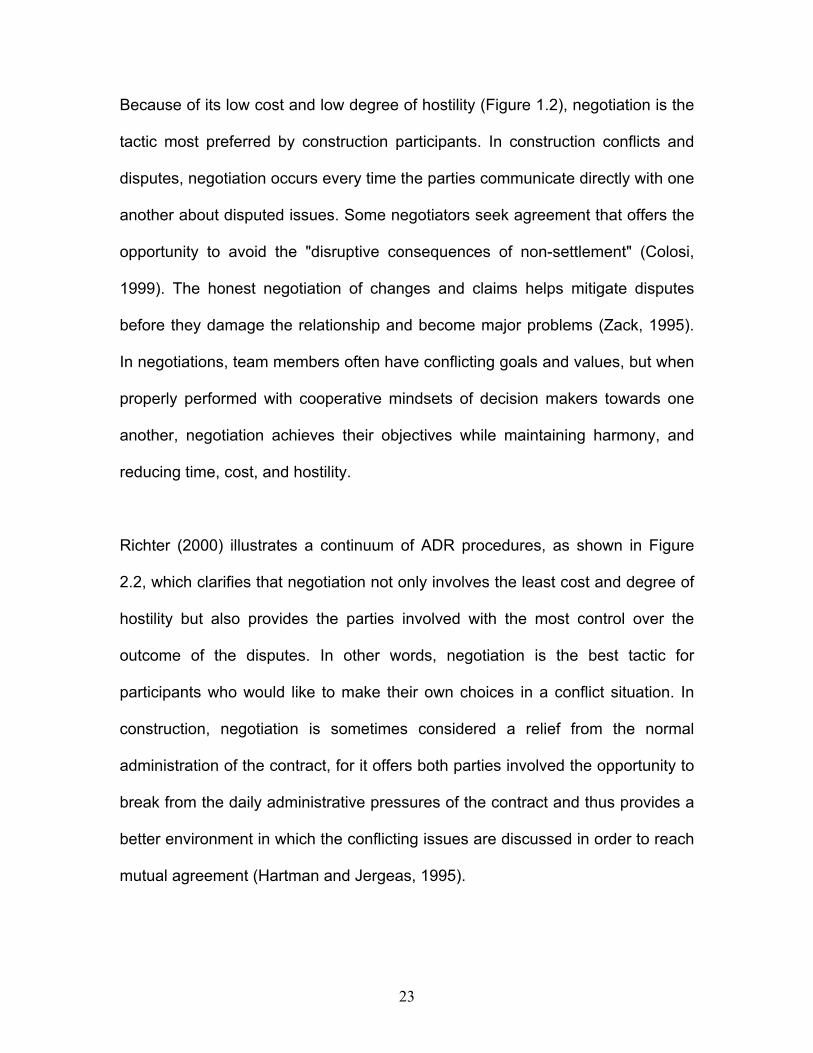
Richter (2000) illustrates a continuum of ADR procedures, as shown in Figure
2.2, which clarifies that negotiation not only involves the least cost and degree of
hostility but also provides the parties involved with the most control over the
outcome of the disputes. In other words, negotiation is the best tactic for
participants who would like to make their own choices in a conflict situation. In
construction, negotiation is sometimes considered a relief from the normal
administration of the contract, for it offers both parties involved the opportunity to
break from the daily administrative pressures of the contract and thus provides a
better environment in which the conflicting issues are discussed in order to reach
mutual agreement (Hartman and Jergeas, 1995).
24
Figure 2.2: Dispute Resolution Continuum (Richter, 2000)
In a negotiation process, effective negotiation skills are a tremendous asset to
any successful executive. They are especially significant for construction
executives who are continually involved in managing and administering complex
contractual relationships involving substantial amounts of money (Jergeas,
2008). However, many individuals often fail in negotiation not because they are
unable to reach an agreement, but because they walk away from the table before
they achieve the results they are capable of obtaining. Moreover, in spite of the
importance of negotiation, proper training in negotiation skills is not provided
within the construction industry. Negotiations are an important activity, but they
are the subject of little research or education (Dudziak and Hendrickson, 1988).

25
Project managers seem to learn negotiating skills only through experience and
observation (Smith, 1992). Therefore, negotiation support tools for the
construction industry may be useful in enabling the participants in a project to
handle negotiation more productively.
2.2.3. Brownfield Negotiation
Brownfield projects are reconstruction projects in which the land has already
been contaminated and the site may contain hazardous materials that pose a risk
to human health and the environment. In Canada, it is estimated that as much as
25% of the land area in major urban centers is potentially contaminated because
of previous industrial activities (Benazon, 1995). Interest on the part of
developers and lending institutions in redeveloping contaminated sites has
tended to be minimal because such projects may involve high cleanup costs that
limit the profit margin. Moreover, developers fear being held liable for any
negative environmental effects that could be traced to the redeveloped site. On
the other hand, these sites are potentially valuable because they are often
located in the core sections of metropolitan areas and thus are prime candidates
for urban redevelopment and renewal (Bourne, 1995; Barnett, 1995). Therefore,
Canadians municipalities and local governments have established
comprehensive programs and incentives in order to facilitate brownfield
remediation and redevelopment with the hope of achieving the objectives and
benefits listed in Table 2.3. It should be mentioned that the listed objectives can
be further completed.

26
Table 2.3: The Objectives of Brownfield Reconstruction (De Sousa, 2000)
Environmental Social Economic
Reduction of development pressure on greenfield sites,
Protection of public health and safety,
Protection of groundwater resources,
Protection and recycling of soil resources,
Restoration of former landscapes, and
Establishment of new areas deemed to have ecological values.
Renewal of urban cores, Elimination of the negative
social stigmas of the affected communities by revitalizing them, and
Reduction of the fear of ill health, environmental deterioration and shrinking property values in these communities.
Attraction of domestic and foreign investment,
Restoration of tax base of government especially at the local level,
Increased utilization of and reinvestment in existing municipal services, and
Development of remediation /decontamination technology
To achieve these objectives, it is essential that government representatives (e.g.,
municipalities) promote cooperation between the current owner(s) of
contaminated sites and potential investor(s) so that the parties may share the
cost as well as the benefits of redeveloping brownfield sites. However, because
of the challenges associated with brownfield reconstruction (e.g., uncertainty
about liability with respect to the chain of title, lender hesitation, the time to
occupancy, community support, the proposed land use, the condition of the local
infrastructure, the support of local politicians, and the availability of financial
incentives), many unexpected events may occur during the remediation process.
Such unexpected events may bring the remediation to a temporary halt, resulting
in delays, cost overruns, and serious conflicts and complex disputes among the
parties involved (Barnett, 1995). In brownfield conflicts, as in many other
controversies, a variety of dispute resolution procedures are available, of which,
as shown in Figure 2.2, negotiation is the most preferred because the local
government, the current owner, and the future purchaser can negotiate a solution

27
in a less costly and less hostile environment. Cooperative negotiation among the
parties involved will contribute to a mutual and sustainable agreement among the
parties, and such agreements may help achieve the objectives of brownfield
reconstruction.
Productive negotiation of the complex conflicting issues in a brownfield project
requires that each party has feasible options for each conflicting issue (e.g., cost
of remediation, extent of liability) and reasonable attitudes towards the other
parties. The parties sitting on the negotiation table must interact with one another
in order to find a proper direction in the negotiation process, so they should
therefore consider the strategic as well as the tactical levels of decision making.
The difficulty is that the negotiation of brownfield issues is complicated and the
parties involved, such as the current owner, are most likely not familiar with
negotiation skills and methodologies. Thus, it is essential to develop appropriate
formal negotiation methodologies for the parties involved in brownfield projects
(Yousefi et al., 2009 and Yousefi et al., 2007).
Due to the complexity of brownfield disputes, the proposed brownfield negotiation
methodologies should assist the decision makers in providing resolutions at both
the strategic and tactical levels of decision making. The strategic level assists the
parties to find the proper direction for further negotiations and the tactical level
provides the parties with specific compromises for each negotiation issue needed
to reach an agreed-upon settlement with respect to each negotiation issue.

28
2.3. Negotiation Support Systems in the Construction Industry
Several cases in the literature discuss the application of Information Technology
and Systems (ITSs) in the construction industry: see, for instance, Aouad and
Price (1994), Aouad et al. (1996), Ngee et al. (1997); O’Brien and Al-Soufi
(1994), and Shash and Al-Amir (1997). They have found that ITSs enable
construction activities to be programmed and executed in a speedy and cost-
effective manner. Many applications that have been impossible in the past are
now feasible, such as a project information management system that can handle
tasks like construction programming and information storage and retrieval.
Spreadsheets were among the earliest information management systems that
had a profound effect on the widespread use of support systems among
construction participants. They have strong features such as their intuitive cell-
based structure and their simple interface that is easy to use even for a first-time
user. Underneath the structure and the interface are a host of powerful and
versatile features, from data entry and manipulation to a large number of
functions, charts, and word processing capabilities (Hegazy, 2002). In order to
increase productivity and versatility, programmability options, a number of add-in
programs, and features that allow Internet connectivity and workgroup sharing,
have been also added to newer spreadsheet versions. Because of their wide
uses particularly among construction professionals and participants,
spreadsheets have proven suitable as a decision support system for developing
computer models that require ease of use, versatility, and productivity, such as

29
those for decision support methodologies. For example, a decision support
system for construction conflict resolution is developed by Kassab et al. (2006)
that uses Ms Excel spreadsheet as the system platform. It should be mentioned
that Ms Excel spreadsheets have been applied successfully in many
infrastructure applications such as planning and cost estimation for highway
projects (Hegazy and Ayed, 1998), Critical Path Method and time-cost trade-off
analysis (Hegazy and Ayed 1999), construction delay analysis (Mbabazi et al.,
2005), infrastructure asset management (Hegazy et al., 2004), and cost
estimation for reconstruction of educational buildings (Yousefi et al., 2008).
Negotiation support systems have recently gained attention in the construction
industry. In particular, construction participants have been motivated to benefit
from the continual growth in the development of the internet and computer
technologies, which has led to increased numbers of electronic negotiation
systems. Electronic negotiations are described as processes that involve
computer and communication technologies in one or more negotiation activities
(Bichler et al., 2003). These technologies include the use of e-mail, internet,
world wide web, multimedia, traditional databases, decision support systems,
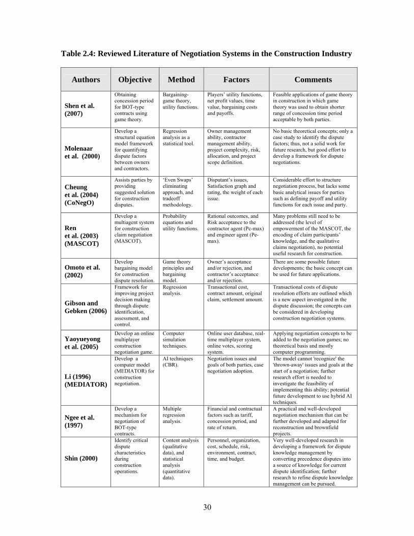
and knowledge-based systems. Table 2.4 summarizes the applications of
negotiation systems in the construction industry and some of these efforts are
briefly explained below. It should be mentioned that the research efforts
summarized in Table 2.4 are based on the available reviewed literature and other
related studies can be added to the list.
30
Table 2.4: Reviewed Literature of Negotiation Systems in the Construction Industry
Authors Objective Method Factors Comments
Shen et al. (2007)
Obtaining concession period for BOT-type contracts using game theory.
Bargaining-game theory, utility functions.
Players’ utility functions, net profit values, time value, bargaining costs and payoffs.
Feasible applications of game theory in construction in which game theory was used to obtain shorter range of concession time period acceptable by both parties.
Molenaar et al. (2000)
Develop a structural equation model framework for quantifying dispute factors between owners and contractors.
Regression analysis as a statistical tool.
Owner management ability, contractor management ability, project complexity, risk, allocation, and project scope definition.
No basic theoretical concepts; only a case study to identify the dispute factors; thus, not a solid work for future research, but good effort to develop a framework for dispute negotiations.
Cheung et al. (2004) (CoNegO)
Assists parties by providing suggested solution for construction disputes.
‘Even Swaps’ eliminating approach, and tradeoff methodology.
Disputant’s issues, Satisfaction graph and rating, the weight of each issue.
Considerable effort to structure negotiation process, but lacks some basic analytical issues for parties such as defining payoff and utility functions for each issue and party.
Ren et al. (2003) (MASCOT)
Develop a multiagent system for construction claim negotiation (MASCOT).
Probability equations and utility functions.
Rational outcomes, and Risk acceptance to the contractor agent (Pc-max) and engineer agent (Pe-max).
Many problems still need to be addressed (the level of empowerment of the MASCOT, the encoding of claim participants’ knowledge, and the qualitative claims negotiation), no potential useful research for construction.
Omoto et al. (2002)
Develop bargaining model for construction dispute resolution.
Game theory principles and bargaining model.
Owner’s acceptance and/or rejection, and contractor’s acceptance and/or rejection.
There are some possible future developments; the basic concept can be used for future applications.
Gibson and Gebken (2006)
Framework for improving project decision making through dispute identification, assessment, and control.
Regression analysis.
Transactional cost, contract amount, original claim, settlement amount.
Transactional costs of dispute resolution efforts are outlined which is a new aspect investigated in the dispute discussion; the concepts can be considered in developing construction negotiation systems.
Yaoyueyong et al. (2005)
Develop an online multiplayer construction negotiation game.
Computer simulation techniques.
Online user database, real-time multiplayer system, online votes, scoring system.
Applying negotiation concepts to be added to the negotiation games; no theoretical basis and mostly computer programming.
Li (1996) (MEDIATOR)
Develop a computer model (MEDIATOR) for construction negotiation.
AI techniques (CBR).
Negotiation issues and goals of both parties, case negotiation adoption.
The model cannot 'recognize' the 'thrown-away' issues and goals at the start of a negotiation; further research effort is needed to investigate the feasibility of implementing this ability; potential future development to use hybrid AI techniques.
Ngee et al. (1997)
Develop a mechanism for negotiation of BOT-type contracts.
Multiple regression analysis.
Financial and contractual factors such as tariff, concession period, and rate of return.
A practical and well-developed negotiation mechanism that can be further developed and adapted for reconstruction and brownfield projects.
Shin (2000)
Identify critical dispute characteristics during construction operations.
Content analysis (qualitative data), and statistical analysis (quantitative data).
Personnel, organization, cost, schedule, risk, environment, contract, time, and budget.
Very well-developed research in developing a framework for dispute knowledge management by converting precedence disputes into a source of knowledge for current dispute identification; further research to refine dispute knowledge management can be pursued.

31
1) Shen et al. (2007) successfully applied bargaining-game theory to obtain
detailed concession periods for construction contracts. Game theory principles
were used particularly to determine specific time spans between moves. In other
words, game theory was employed as a complementary technique for the
methodologies that help decision makers with strategic decisions (i.e., to
determine a broader range for the concession period). The paper, however, did
not consider all the factors (e.g., political, risk attitude, reputation, and
contractor’s economic condition) that may influence the outcome of bargaining.
Nevertheless, with improvements, the technique used in this research has
potential benefits for use in the negotiation of construction disputes.
2) Molenaar et al. (2000) developed a systematic framework for quantifying
dispute factors. The purpose of the research was to explain how and why
contract-related construction problems occur: logistic regression was used to
model the likelihood of construction disputes arising. This study provides a
methodology for quantifying contract disputes. In game theory, these issues are
considered in terms of cardinal and quantified values.
3) Cheung et al. (2004) developed a construction negotiation support system,
namely CoNegO, which assists parties by providing a suggested solution for a
construction dispute. In CoNegO, the communication component is the Internet,
and the data accessibility component manages the sharing of information. The
negotiators first study the construction dispute case and then formulate the
32
bargaining ranges for each issue using two cardinal values: the pessimistic value
represents the baseline of the negotiator with respect to a particular issue (no
further concession will be offered beyond this value) and the optimistic value
represents the value that produces the highest satisfaction for the negotiator.
Negotiators must also determine other parameters for each issue, such as
relative importance and satisfaction rating. Although the research provides a
valuable approach to a negotiation methodology, it is based on the subjective
evaluation of the negotiators. For example, a negotiator may exaggerate his or
her position to provide a better negotiation position, or either or both parties may
inflate their opening demands, misrepresent their positions or interests, withhold
sensitive or potentially damaging information, or use threatening behavior. These
issues need to be addressed.
4) Ren et al. (2003) developed a system specifically for construction claims
called MASCOT that utilizes utility theory. Each party is assigned a linear utility
function which can be determined by two points: the optimum point and the
reservation point. Each party can then estimate the opponent’s utility function
based on these two critical points. The proposed methodology was developed
based on many constraints and idealized assumptions, including quantitative
negotiation, rationality, and fixed utility function. These assumptions decrease the
accuracy of the outcomes produced by this system. The research also provides
some future work to improve the system.
33
5) Yaoyueyong et al. (2005) developed an online multiplayer construction
negotiation game called Virtual Construction Negotiation Game (VCON), as an
innovative tool for negotiation training in the construction industry. In their
research, the procedure for developing an Internet-based negotiation system is
clearly explained, and the ideas can be used in the development of future
computer support systems. Development of the VCON game can be classified
into four major phases: the identification of game requirements, system design,
software development, and system testing. The drawback of this system, as with
many other developed systems, is that the behavioral aspects of decision making
(negotiating), particularly the changes in the attitudes of the negotiators during
the negotiation, are not taken into account.
6) Li (1999) designed MEDIATOR a computer system for construction
negotiation, which employs a Case-Based Reasoning (CBR) technique to
provide intelligent support for construction negotiations. CBR uses previous
cases as a basis for addressing new problems. In contrast to conventional expert
systems (ESs) that use compiled knowledge in problem solving, the system
selects similar cases to help solve a given negotiation problem. The selected
cases are then modified and adapted to generate proposals that should move
negotiators towards a settlement. The system uses three techniques to modify
and transform selected cases in an attempt to generate new proposals: modify
the reservation values, introduce new issues and goals, and select additional
cases. Although the research tried to use Artificial Intelligence techniques (e.g.,
34
CBR) in developing a negotiation methodology, there are significant difficulties in
using CBR, for example, in collecting previous negotiation cases. Direct
collection is difficult because negotiation history is seldom recorded and
documented. Hence, it is very difficult to reconstruct and understand how the
results of the negotiation were arrived at. Another difficulty in using CBR lies in
capturing the original context of a negotiation. In other words, in special
economic and political conditions, negotiators may make concessions at any cost
in order to win with respect to specific issues. When a negotiation case for a
problem is reused in a different economic climate, it is necessary to know the
initial context so that it can be adapted consistently. Therefore, one should be
cautious in using CBR or other AI techniques that use historical data as input to
the model.
The above studies provide important insights into the application of negotiation
support systems in the construction industry. A variety of decision-making
techniques have been used, and many studies have been carried out in order to
make sure that the decision-making models are as accurate as possible.
However, the study of available negotiation systems reveals that other aspects of
decision making need to be considered. For example, the behavioral
characteristics of the involved parties are not formally considered in the dispute
negotiation process when many of the negotiation support tools are developed.
The attributes of each party play a significant role in modeling a negotiation
process since the attitude of decision makers is the most influential psychological
35
aspect that can change the outcome of negotiation. For example, it is vital to
consider each party’s attitudes toward risk in order to assign a utility function to
the player. Decision-making systems can also be enhanced by integrating the
strategic level of decision making with the detailed (tactical) level of negotiation.
As Fisher et al. (1991) emphasize, any negotiation takes place at two levels. The
first level involves “negotiation of the substantive issues” (e.g., contract price).
The next level of negotiation refers to “the procedure for dealing with the
substantive issues”. This “upper” level dictates how each side plays the game of
negotiation. For instance, one can negotiate by hard positional bargaining, by a
cooperative approach, or by another method (Fisher et al., 1991).
The objective for the research in this thesis is the development of a systematic,
reliable, and sustainable negotiation methodology that is suitable for application
to complex construction disputes and that incorporates the behavioral aspects of
construction professionals and participants not only at the strategic level of
decision making but also at the tactical level. Because negotiation is an important
aspect of decision making, it is, therefore, essential to review decision-making
concepts, techniques, approaches, and methodologies in some depth as shown
in the remainders of this chapter.
2.4. Decision Making
Decision making is the process of choosing a preferred option or course of action
from among a set of alternatives (Raiffa et al., 2002). Decision making permeates
36
all aspects of life: people must decide what to buy, whom to vote for, what job to
take, and so on. Decisions often involve uncertainty about the external world
(e.g., What will the weather be like?), as well as conflict regarding one’s own
preferences (e.g., Should I opt for a higher salary or for more leisure?). The
decision-making process often begins at the information-gathering stage and
proceeds through likelihood estimation and deliberation, until the final act of
choosing (Bell et al., 1988).
Engineering decision making can also be grouped into two extreme levels: the
strategic level and the tactical level, as shown in Figure 2.3. The flowchart on the
left side of Figure 2.3 contains the main factors that must be considered in the
selection of a suitable model for an engineering problem. In addition to proper
engineering modeling, any alternative solution must be assessed with respect to
environmental, economical and financial, and political and social feasibility (Hipel
and Fang, 2005). Appropriate techniques from systems engineering and
operational research can assist with these evaluations throughout the decision-
making process. The top cell on the left in Figure 2.3 indicates that output from
all of the analyses provides information to assist decision makers in making an
eventual overall decision (Hipel et al., 2007).
The right-hand portion of Figure 2.3 depicts the characteristics that are embodied
in the hierarchical framework of the engineering decision-making process. It
should be noted that as one moves from the tactical level of decision making to
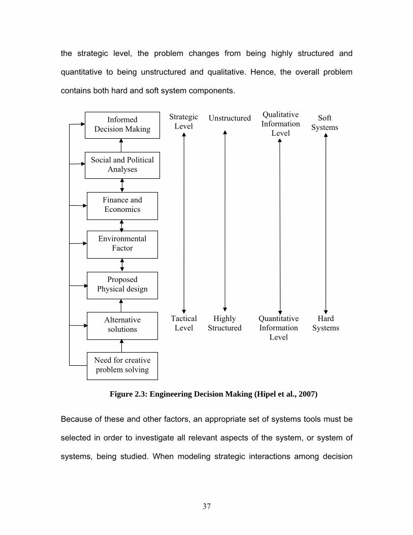
37
the strategic level, the problem changes from being highly structured and
quantitative to being unstructured and qualitative. Hence, the overall problem
contains both hard and soft system components.
Because of these and other factors, an appropriate set of systems tools must be
selected in order to investigate all relevant aspects of the system, or system of
systems, being studied. When modeling strategic interactions among decision
Finance and Economics
Social and Political Analyses
Figure 2.3: Engineering Decision Making (Hipel et al., 2007)
Environmental Factor
Proposed Physical design
Alternative solutions
Need for creative problem solving
Tactical Level
Highly Structured
Quantitative Information
Level
Hard Systems
Unstructured Strategic Level
Soft Systems
Informed Decision Making
Qualitative Information
Level
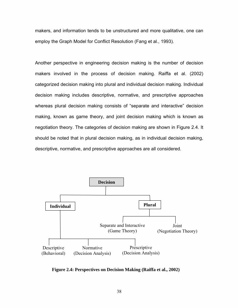
38
makers, and information tends to be unstructured and more qualitative, one can
employ the Graph Model for Conflict Resolution (Fang et al., 1993).
Another perspective in engineering decision making is the number of decision
makers involved in the process of decision making. Raiffa et al. (2002)
categorized decision making into plural and individual decision making. Individual
decision making includes descriptive, normative, and prescriptive approaches
whereas plural decision making consists of “separate and interactive” decision
making, known as game theory, and joint decision making which is known as
negotiation theory. The categories of decision making are shown in Figure 2.4. It
should be noted that in plural decision making, as in individual decision making,
descriptive, normative, and prescriptive approaches are all considered.
Decision
Individual Plural
Separate and Interactive (Game Theory)
Joint (Negotiation Theory)
Descriptive (Behavioral)
Normative (Decision Analysis)
Prescriptive (Decision Analysis)
Figure 2.4: Perspectives on Decision Making (Raiffa et al., 2002)
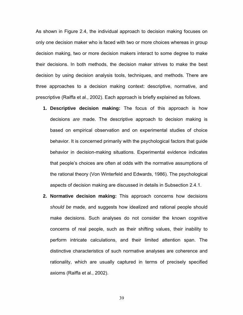
39
As shown in Figure 2.4, the individual approach to decision making focuses on
only one decision maker who is faced with two or more choices whereas in group
decision making, two or more decision makers interact to some degree to make
their decisions. In both methods, the decision maker strives to make the best
decision by using decision analysis tools, techniques, and methods. There are
three approaches to a decision making context: descriptive, normative, and
prescriptive (Raiffa et al., 2002). Each approach is briefly explained as follows.
1. Descriptive decision making: The focus of this approach is how
decisions are made. The descriptive approach to decision making is
based on empirical observation and on experimental studies of choice
behavior. It is concerned primarily with the psychological factors that guide
behavior in decision-making situations. Experimental evidence indicates
that people’s choices are often at odds with the normative assumptions of
the rational theory (Von Winterfeld and Edwards, 1986). The psychological
aspects of decision making are discussed in details in Subsection 2.4.1.
2. Normative decision making: This approach concerns how decisions
should be made, and suggests how idealized and rational people should
make decisions. Such analyses do not consider the known cognitive
concerns of real people, such as their shifting values, their inability to
perform intricate calculations, and their limited attention span. The
distinctive characteristics of such normative analyses are coherence and
rationality, which are usually captured in terms of precisely specified
axioms (Raiffa et al., 2002).

40
3. Prescriptive decision making: This approach focuses on how decisions
could be made better. The question the prescriptive analyses ask is what
a real person can actually do to make better decisions. In seeking to craft
useful theory, prescriptive analyses do not take into consideration
conceptual ideas and techniques that are useful for idealized, mythical,
and super-rational people. Instead, prescriptive proposals must be useful
for real people. Because real people are different, good advice has to be
tuned to the different needs, capabilities, and emotional makeup of the
individuals for whom the prescriptive advice is intended (Bell et al., 1988).
Prescriptive advice should be evaluated based on its pragmatic value and
its ability to help people make better decision. Advice should also promote
an understanding of the problems, confidence in the decisions, justification
for the decisions, and satisfaction with the consequences. Prescriptive
analysis should be informed by descriptive and normative theories (Raiffa
et al., 2002).
2.4.1. The Psychological Aspects of Decision Making
Psychological factors such as human perception, emotion, attention, attitude, and
effort are certain to influence decision making. Despite economists’ assumptions
about the perfect rationality of people when they make decisions, the fact is that
people often have faulty intuition about their own motives and behaviors, and
they often act to bring about outcomes that they themselves judge to be bad
(Kahneman and Tversky, 2000). Psychologically, people experience conflict and
41
behave differently when they face decision making. They often approach
decisions as they would problem-solving tasks, trying to gauge the various
attributes and come up with compelling arguments for choosing one option over
another. At times, a comparison of the alternatives yields compelling reasons to
choose one option. At other times, the conflict between the available alternatives
is hard to resolve, which can lead the decision maker to seek additional options
or to maintain the status quo. This behavior has implications that are not readily
apparent: people sometimes need to decide whether to opt for an available
option or to search for additional alternatives (Camerer, 1995). Psychological
studies of decisional conflict (e.g., Kagel and Roth, 1995; Morley, 1981; Yousefi,
et al., 2008; Rabin, 1998) suggest that people are more likely to opt for an
available option when they have a compelling reason that makes the decision
easy, and that they are tempted to delay the decision and search further when a
compelling reason is not readily available and the decision is hard to make.
Conflict, on the other hand, plays no role in the classical analysis, according to
which a person is expected to search for additional alternatives if the expected
value of searching exceeds that of the best option currently available. Important
psychological aspects of decision making are summarized in Table 2.5
2.4.2. Attitudes and Utility Theory in Decision Making
Attitude is defined by Krech et al. (1962) as “an enduring system of positive or
negative evaluations, emotional feelings and pro and con action tendencies, with
respect to a social object”. In other words, the attitude is a preparation in
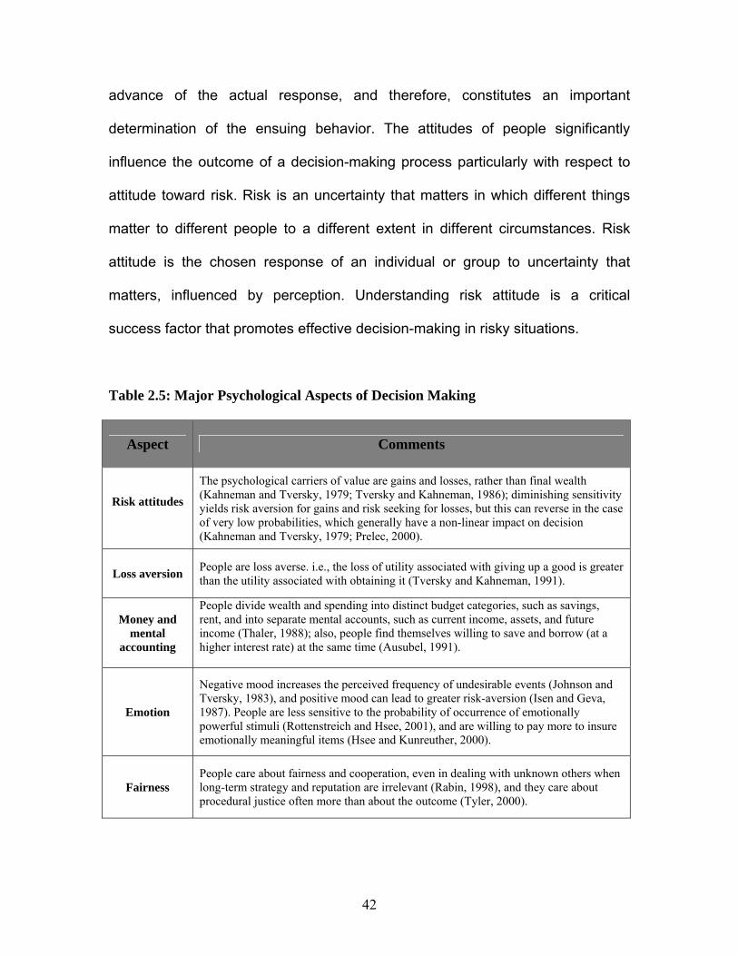
42
advance of the actual response, and therefore, constitutes an important
determination of the ensuing behavior. The attitudes of people significantly
influence the outcome of a decision-making process particularly with respect to
attitude toward risk. Risk is an uncertainty that matters in which different things
matter to different people to a different extent in different circumstances. Risk
attitude is the chosen response of an individual or group to uncertainty that
matters, influenced by perception. Understanding risk attitude is a critical
success factor that promotes effective decision-making in risky situations.
Table 2.5: Major Psychological Aspects of Decision Making
Aspect Comments
Risk attitudes
The psychological carriers of value are gains and losses, rather than final wealth (Kahneman and Tversky, 1979; Tversky and Kahneman, 1986); diminishing sensitivity yields risk aversion for gains and risk seeking for losses, but this can reverse in the case of very low probabilities, which generally have a non-linear impact on decision (Kahneman and Tversky, 1979; Prelec, 2000).
Loss aversion
People are loss averse. i.e., the loss of utility associated with giving up a good is greater than the utility associated with obtaining it (Tversky and Kahneman, 1991).
Money and mental
accounting
People divide wealth and spending into distinct budget categories, such as savings, rent, and into separate mental accounts, such as current income, assets, and future income (Thaler, 1988); also, people find themselves willing to save and borrow (at a higher interest rate) at the same time (Ausubel, 1991).
Emotion
Negative mood increases the perceived frequency of undesirable events (Johnson and Tversky, 1983), and positive mood can lead to greater risk-aversion (Isen and Geva, 1987). People are less sensitive to the probability of occurrence of emotionally powerful stimuli (Rottenstreich and Hsee, 2001), and are willing to pay more to insure emotionally meaningful items (Hsee and Kunreuther, 2000).
Fairness People care about fairness and cooperation, even in dealing with unknown others when long-term strategy and reputation are irrelevant (Rabin, 1998), and they care about procedural justice often more than about the outcome (Tyler, 2000).

43
A decision maker who prefers to receive an expected value for certain rather
than an uncertain alternative is called risk averse, while someone who finds
receiving the expected value for certain to be equally preferred to the alternative
is called risk neutral, and someone who prefers to receive the uncertain
alternative rather than the expected value for certain is called risk seeking. In
order to manage risk attitude, four steps can be considered (Kahneman and
Tversky, 1979; Tversky and Kahneman, 1986):
1. Awareness: Of how perception of a risky situation will shape risk attitude
and behaviour,
2. Appreciation: More than understanding, respect for differing views as a
basis for engaging and changing if necessary,
3. Assertion: Needs and issues will need to be articulated if risk attitude is to
change, and
4. Action: Willingness to take action and be resilient in the pursuit of goals,
beyond ‘good intentions’
Utility theory is an attempt to infer subjective value, or utility, from choices. Utility
theory can be used in both decision making under risk (where the probabilities
are explicitly given) and in decision making under uncertainty (where the
probabilities are not explicitly given). Extensions of utility theory include
subjective probability as well as distortions of probability (Bell et al., 1988).
Because utility theory is dealing with preferences, it is often convenient to
represent preferences with a utility function and reason indirectly about

44
preferences with utility functions. Therefore, many types of utility functions have
been proposed and more discussion in this regard is provided in Chapter 6.
A decision maker's attitude toward risk taking determines the shape of his or her
utility function. Knowing that a decision maker is risk averse can substantially
restrict the shape of a utility function (Kirkwood, 1997). These varying levels of
attitude toward risk can be expressed as exponential functions. The exponential
utility function can be expressed as follows (Kirkwood, 1997).
,...................................)(
................1]/)(exp[
1]/)(exp[)(
OtherwiseLowHigh
Lowxxu
InfinityIfLowHigh
Lowxxu
−−
=
≠−−−
−−−= ρ
ρρ
In the above equations, “Low” is the lowest level of “x” that is of interest, “High” is
the highest level of “x”, and “ρ” is the risk tolerance for the utility function. Figure
2.5 shows examples of exponential utility functions for different risk tolerances
(ρ). In both parts of this figure, the range of values for the evaluation measure is
from Low = 0 to High = 10. Part “a” of the figure shows functions with increasing
preferences (e.g., reconstruction profit for a contractor), and part “b” shows
functions with decreasing preferences (e.g., cost sharing for the involved parties)
(Kirkwood, 1997). In Figure 2.5a, for example, the function shape with ρ = 1
represents a very risk-averse decision maker, whereas the function shape with ρ
= -1 represents a very risk-taking decision maker. The unlabeled straight line in
the center of each part of the figure corresponds to the case when ρ = Infinity,
which means that a decision maker is risk-neutral. Figure 2.5 also shows that as

45
the magnitude of the risk tolerance increases, the utility function becomes more
linear.
The above concepts have been also used to develop decision-making support
systems. In a research attempt to incorporate the attitude of decision makers to a
negotiation system using utility function, Ji et al. (2007) developed an attitude-
adaptation negotiation model that assigned a utility function to each negotiator
when they interactively negotiate one or several issues in an electric market. To
enable agents to adapt their attitudes according to negotiation duration, utility
function was constructed on the basis of a history-adaptation strategy and the
fixed-attitude strategies were compared by simulation. Also, in another research
effort, Zhang et al. (2005) used multi-dimensional utility function to develop a
cooperative negotiation mechanism for multi-agent systems. This mechanism
uses marginal utility gain and marginal utility cost to structure the negotiation
process. The idea of multi-dimensional utility function allows decision makers to
negotiate over multiple attributes of the commitments which make it more likely
0 2 4 6 8 10
Utility
0.0
0.5
1.0
0 2 4 6 8 10
Utility
0.0
0.5
1.0
b. Decreasing Preferences a. Increasing Preferences
ρ = 1 ρ = 1 ρ = 5
ρ = 5 ρ = -5 ρ = -5
ρ = -1 ρ = -1
Figure 2.5: Exponential Utility Functions (Kirkwood, 1997)

46
for decision makers to find a solution that increases the global utility by producing
more options.
With respect to analyzing and modeling, group decision making is more
complicated than individual decision making because decision makers possess
different interests, attitudes, goals, and preferences, and each party tries to
achieve his or her own interests and objectives. The process of group decision
making consists of offers and counteroffers by decision makers in a specific
manner which constitutes the dynamics of decision making. Therefore, the study
of interactions among decision makers is of key importance in analyzing group
decision making. Two broadly defined methodologies have been developed for
studying group decision making: game theory and negotiation analysis.
2.5. Game Theory
Game theory is the mathematical study of interactions among decision makers,
or players. Known as interactive decision making, game theory is an approach to
study how to construct different kinds of games as models of real-world decision
problems and how to analyze and interpret them. It has been applied to a broad
range of fields, including economics, political science, biology, psychology,
linguistics, systems engineering, and computer science (Hipel, 2008 a, b; Hipel
and Ben-Haim, 1999; Sage and Rouse, 1999). It should be remembered that in
games, as in other models, some details are inevitably missing; however, games
are useful since they facilitate the study of some aspects of interactive decisions,
47
while ignoring others. Of course, the model is not the real situation, so what is
learned is limited, but often studying the models provides players with surprising
insights (Kilgour, 2006). Game theory was initially introduced by Von Neumann
and Morgenstern in their book Theory of Game and Economic Behavior (Von
Neumann and Morgenstern, 1944 and 1953). This section introduces basic game
theory, which is referred to in the remainder of this thesis.
2.5.1. Game Theory in Conflict Analysis
Game theory contributes significantly to the study of the various types of
conflicts. The application of game theory in conflict resolution is explained in an
overview paper by Hipel (2003) and in a series of articles about Conflict
Resolution in the Encyclopedia of Life Support Systems (EOLSS) (2002), as well
as in two edited books by Hipel (2008 a, b). Figure 2.6 shows the genealogy of
formal models for analyzing conflict which are based on a number of underlying
assumptions. As shown in Figure 2.6, in the quantitative approach, cardinal
preferences are to be determined whereas in the non-quantitative approach, only
relative preference information is required. It is very hard sometimes to obtain
cardinal preferences for the disputants involved in societal disputes. Therefore,
non-quantitative approaches are especially useful for formally studying social and
environmental conflicts and disputes because of their inherent qualitative nature.
Both quantitative and non-quantitative approaches are described in the following
subsections.

48
2.5.2. Quantitative Approach to Game Theory
Quantitative game theory is broadly divided into two distinct classes: non-
cooperative and cooperative games, as shown in Table 2.6. The distinction has
to do with the kinds of interacting choices the players make. In non-cooperative
games, the general principle is that only those aspects of the players’ interaction
that are explicitly included in the model are to be taken into account, and players
act in their own best interests. In cooperative games on the other hand, not only
can players communicate, but they also have access to a reliable and cost-free
mechanism, that enables them to make binding agreements at no cost. In other
words, the question in cooperative games is not so much whether the players will
cooperate, but how they will share the benefits of cooperation (Kilgour, 2006;
Von Neumann and Morgenstern, 1953).
Game Theory
Quantitative Approaches
Normal Form
Conflict Analysis
Graph Model for Conflict Resolution
Figure 2.6: Genealogy of Formal Conflict Models (Based on Hipel and Fang, 2005)
Non-quantitative Approaches
Extensive Form
Metagame Analysis Cooperative
Game Theory Drama Theory

49
Table 2.6: Game Theory Classification (based on Kilgour, 2006)
Non-Cooperative
Complete Information Incomplete Information Cooperative
Stat
ic
Strategic-Form Games
Strategic-Form
Games
Dyn
amic
Extensive-Form Games
Extensive-Form Games
Cooperative Games
It is noted that, in the real world, most human interactions lie somewhere
between non-cooperative and cooperative, and are usually not at either extreme.
However, to analyze and model real-world problems using game theory
approaches, it is important to know both extremes, not only because they are
relatively easy to formulate and study, but also because the behavior observed,
predicted, or recommended at the two extremes is a kind of benchmark for what
can be expected in the real world.
2.5.2.1. Concepts and components of quantitative game theory
Conceptually, game theory is in essence interactive decision making that
involves a set of individual players who have a specified set of choices and the
payoff (utility) to each player depends on the totality of the choices made by all
players. Each player must choose, sometimes not knowing the choices of the
others. Each player must consider what the others might do and realize that the
others are, in turn, considering what the others are thinking. The essence of this
perspective is that although the individual players make their choices separately

50
from each other, the payoffs they receive are a function of all players’ choices.
The expected utility hypothesis is widely accepted in the field of game theory.
The hypothesis states that when faced with uncertainty about which outcomes he
or she will receive, the player prefers outcomes that maximize his or her
expected utility.
Each game is played by a finite set of players. Players may be an entity or a
group of people who are economically rational. That is, players can assess
outcomes, calculate path(s) to outcomes, and choose actions that yield their
most preferred outcomes (Morris, 1994). After the game ends, each player
receives a numerical payoff. This number may be negative, in which case it is
represented as a loss of the absolute value of the number. To study a game that
has psychological payoffs (e.g., happiness, satisfaction, prestige), it is necessary
to replace the non-quantitative payoffs with numerical ones (Morris, 1994). A
strategy is also a predetermined logic that tells a player which actions to take in
response to every possible strategy other players might use and which action
should not be taken. Each player in the game faces a choice of two or more
possible strategies that must be selected by the player who seeks maximum
level of satisfaction for his or her chosen strategy.
2.5.2.2. Cooperative game theory
Cooperative game theory describes only the outcomes that result when the
players come together in different combinations. In cooperative games, players
51
can and do communicate and, moreover, have a reliable and cost-free
enforcement mechanism that enables them to make binding agreements at no
cost. The enforcement mechanism is external to the game (i.e., not explicitly
modeled). In cooperative games, the question is not whether the players will
cooperate in their common interest, but how they will share the gains of
cooperation (Kilgour, 2006).
A game theory approach to bargaining was first introduced by Nash (1950) and
Nash (1951), who developed a cooperative and static game model. In a two-
person bargaining problem, two players have access to a set of alternatives,
which is called the feasible set. It is assumed that each player has preferences
over the alternatives and that the preferences are represented by two functions,
u1 and u2. In the original approach by Nash, as in many later developments, it
has been assumed that these utility functions are Von Neumann-Morgenstern
utilities. The utility functions, u1 and u2, define a subset S of R2, which is the
image of the set of feasible alternatives. Each point of S represents a solution for
the bargaining problem that is an agreement between the players. Within the
feasible set there is also a point called the threat point or disagreement point (d),
which is the point at which the game ends and no agreement can be reached.
Therefore, a two-person bargaining problem is a pair (S, d) such that S is
convex, closed (i.e., it contains its boundary), and a comprehensive subset of R2;
and d Є S, and there exists at least one x Є S such that x > d. There are also two

52
main bargaining solutions: the Nash solution and the Kalai-Smorodinski (K-S)
solution, which are further explained by Kilgour (2006).
2.5.3. Non-quantitative Approach to Game Theory
Because social conflicts tend to be non-quantitative in nature, many studies have
been carried out using techniques listed in the left branch in Figure 2.6. For
example, Howard published a pioneering book on metagame analysis (Howard,
1971). Metagame analysis provides a theoretical basis for modeling the dynamic
aspects of conflict based on the metaphor of a drama, which is another useful
non-quantitative methodology (Howard, 1999; Bryant, 2003). Fraser and Hipel
(1984) explain the scope of metagame analysis further in a systematic process
called conflict analysis, which provides an analytical and formal platform for
developing graph model for conflict resolution (Fang et al., 1993). It should be
mentioned that the Graph Model for Conflict Resolution (GMCR) is completely
discussed in Chapter 3.
2.6. Negotiation Overview
Negotiation is a process by which two or more parties conduct communications
or conferences with a view to resolving differences between them (Cohen, 2002).
Negotiation analysis is known as joint decision making. In contrast with
cooperative game theory in which the players should achieve mutual benefits
and decide how their gains are to be split up, the negotiation analysis involves
multiple individuals cooperating to arrive at one joint decision (Kilgour, 2006).

53
The joint decision entails joint consequences, or payoffs, for each individual. It
should be noted that underlying every negotiation structure is a game-like
component, and the more one studies negotiations, the more one realizes the
artificiality of the borders between the two perspectives (Raiffa et al., 2002).
Raiffa also believed that negotiation is considered to be both art and ability. On
one hand, negotiation is an art which requires the deliberate application of
techniques and strategies aimed at a specific goal. This goal is expressed as the
equitable adjustment of an impacted contract based on time and cost. On the
other hand, the ability of engineers and managers to negotiate effectively is
crucial to the success or failure of the project.
2.6.1. Bargaining and Negotiation
Bargaining is a type of negotiation in which two or more decision makers usually
negotiate over only one issue. For example, the buyer and seller of goods or
services bargain over the price that will be paid and the exact nature of the
transaction that will take place, and eventually come to an agreement. Bargaining
thus is an alternative pricing strategy to fixed prices. Decision makers in a
bargaining problem can bargain over the objective (e.g., project duration) as a
whole at any precise moment in time. The problem can also be divided so that
parts of the whole objective become subject to bargaining during different stages.
In a bargaining problem, the result is either an agreement between the interested
parties or the status quo of the problem. It is clear that studying how individual

54
parties make bargaining decisions is insufficient for predicting which agreement
will be reached.
Bargaining can be either cooperative or non-cooperative. Cooperative bargaining
refers to the cooperative character of the strategic interaction that takes place in
the decision-making process. Most definitions and conceptualizations of
cooperation in bargaining are focused on the reaching of an agreement
(Myerson, 1991; Young, 1991). In other words, cooperative bargaining is defined
as working or acting together willingly for a common purpose or benefit in the
presence of conflicting interests (Fearon, 1995; Muthoo, 1999). Therefore,
cooperatively bargaining over one issue is one of the important topics in the
study of negotiation (Sebenius, 1992). Dunlop (1984) presented four approaches
to bargaining:
1. Seek to explain bargaining generally and collective bargaining
negotiations in particular.
2. Use experimental or simulated bargaining games in order to determine the
bargaining outcomes.
3. Use econometric methods to measure aspects of arbitration or collective
bargaining. Public-sector bargaining has been used most often because of
the availability of data.
4. Use a word-by-word account of the exchanges from the earliest stages of
negotiation to the achievement of a settlement.
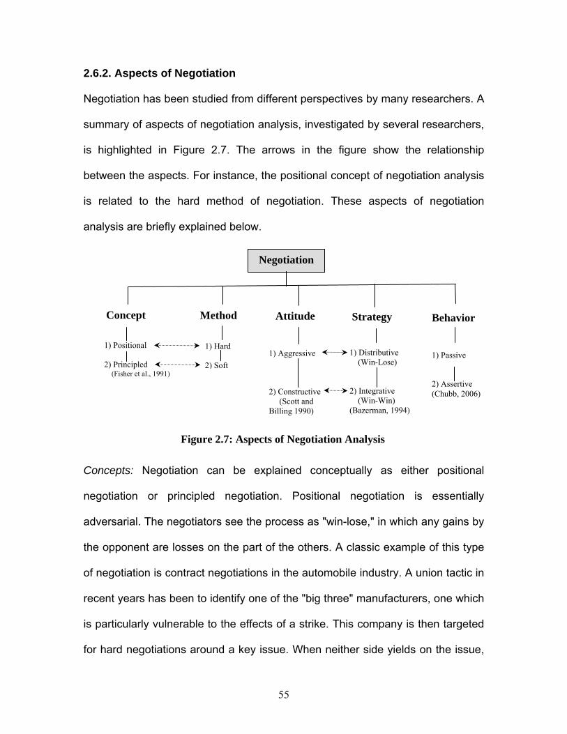
55
2.6.2. Aspects of Negotiation
Negotiation has been studied from different perspectives by many researchers. A
summary of aspects of negotiation analysis, investigated by several researchers,
is highlighted in Figure 2.7. The arrows in the figure show the relationship
between the aspects. For instance, the positional concept of negotiation analysis
is related to the hard method of negotiation. These aspects of negotiation
analysis are briefly explained below.
Concepts: Negotiation can be explained conceptually as either positional
negotiation or principled negotiation. Positional negotiation is essentially
adversarial. The negotiators see the process as "win-lose," in which any gains by
the opponent are losses on the part of the others. A classic example of this type
of negotiation is contract negotiations in the automobile industry. A union tactic in
recent years has been to identify one of the "big three" manufacturers, one which
is particularly vulnerable to the effects of a strike. This company is then targeted
for hard negotiations around a key issue. When neither side yields on the issue,
Negotiation
Concept Behavior Method Strategy
1) Positional 2) Principled (Fisher et al., 1991)
1) Passive 2) Assertive (Chubb, 2006)
1) Distributive (Win-Lose) 2) Integrative (Win-Win) (Bazerman, 1994)
1) Hard 2) Soft
Figure 2.7: Aspects of Negotiation Analysis
Attitude
1) Aggressive 2) Constructive (Scott and Billing 1990)
56
a strike ensues and persists until an agreement is reached or one side collapses
under the cost of the strike. Although there might be definite winners and losers
in this type of negotiation, it may consequently be beneficial for the parties
involved. Principled negotiation, on the other hand, emphasizes that the parties
involved look for mutual gains. The theory relies on separating the people from
the problem, in an attempt to avoid the human issues that can bias a negotiation
(Fisher et al., 1991). Hence, principled negotiation implies a level of disputant
rationality. Principled negotiation, as suggested by its title, focuses on the
underlying values (or interests) that justify disputants’ positions, as opposed to
attempting negotiation solely from their positions. Keeney (1992) supported the
idea of principled negotiation by proposing value-based negotiation. Value-based
negotiation is an alternative negotiation strategy that challenges positional
negotiation by proposing that understanding the values disputants place on
issues is more important in making decisions than staking out the positions
(Keeney, 1992). In value-based negotiation, negotiators try to increase the
number of alternatives for resolving the disputing issues and start negotiation by
isolating several alternatives to be considered. Fall-back bargaining, for example,
is an alternative-based negotiation that focuses on negotiation that produces a
prediction about the negotiation outcome (Brams and Kilgour, 2001). Negotiators
are begun by insisting on their most preferred alternatives, then falling back, in
lockstep, to less and less preferred alternatives until there is an alternative with
sufficient support. The outcome of fallback bargaining is a subset of alternatives
called the compromise set. This set may be compared to the product of a social

57
choice rule. Another alternative-based algorithm is the Even Swaps method
(Hammond et al., 1999), in which disputants commence negotiations by isolating
several alternatives under consideration. During negotiation, the preferences of
the parties move towards one or a combination of the alternatives. At this stage,
it is assumed that the disputants have agreed on an alternative or a group of
alternatives to form the basis of a settlement.
Methods: Two methods of negotiation can be distinguished: hard and soft. Hard
negotiation strategies emphasize results over relationships. Hard negotiators
insist that their demands be completely agreed to and accepted before any
agreement is possible. While this approach avoids the need to make
concessions, it also reduces the likelihood of successfully negotiating an
agreement and usually harms the relationship with the other party as well. Soft
negotiation on the other hand, seeks agreement at almost any cost, with the
parties offering concessions easily in the interests of preserving (or creating) a
good relationship with the other side. Soft negotiators trust the other side and are
open and honest about their bottom line. This strategy however, leaves the soft
negotiators vulnerable to the hard negotiators who act competitively (Lax and
Sebenius, 1992). However, two hard negotiators competing against each other
may both lose; hence, the advice to negotiate hard in all cases is not wise. Fisher
et al. (1991) suggested that principled negotiation, which negotiates interests
rather than positions, is a better alternative than either hard or soft negotiation.
58
Attitudes: Negotiators’ attitudes play an unavoidable role in the outcome of
negotiation. Negotiators with aggressive (i.e., negative) attitudes toward other
negotiators usually believe in the hard method of negotiation in which
concessions are almost non-existent. On the other hand, negotiators who
possess constructive (i.e., positive) attitudes are encouraged to follow the soft
method of negotiation by making concessions with respect to disputing issues.
With constructive attitudes, negotiators share their concerns and interests
positively and try to agree on a win-win and mutual solution which would be
better than leaving the negotiation table with no resolution of the conflict (Scott
and Billing, 1990). In aggressive negotiation, the parties involved often have
negative attitudes toward one another and they consider any concession made
as a positive improvement for their opponents.
Strategies: Negotiation strategies are divided into two categories: distributive
(claiming the pie) and integrative (enlarging the pie of available resources),
according to Bazerman (1994). The distributive strategy of negotiation is a zero-
sum game; that is, one party’s gain results in the other’s loss. The strategy for
such a negotiation is to predict the bottom line of the other and present an offer
that will maximize one’s own benefit. Such negotiation usually results in a lower
satisfaction level. On the other hand, the integrative strategy promotes
cooperation between the negotiators. Because each negotiator has different
preferences for each negotiable issue and option, the strategy is not to win on all
issues, but to realize which issues the negotiators care most about and make
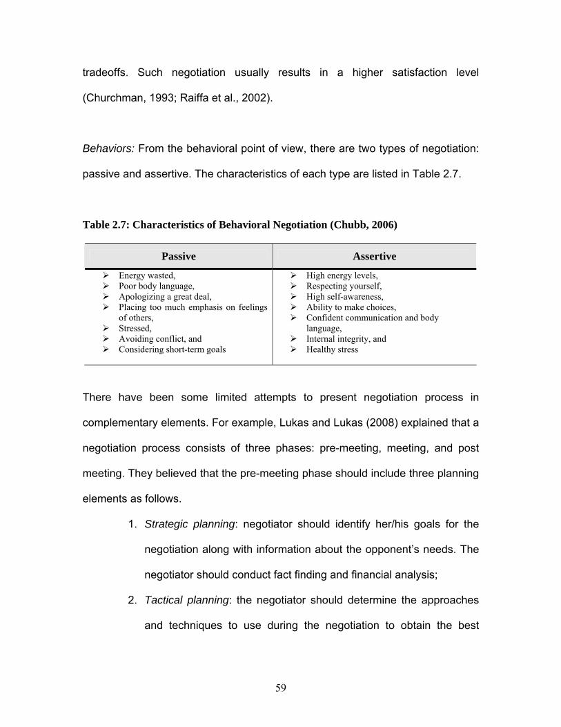
59
tradeoffs. Such negotiation usually results in a higher satisfaction level
(Churchman, 1993; Raiffa et al., 2002).
Behaviors: From the behavioral point of view, there are two types of negotiation:
passive and assertive. The characteristics of each type are listed in Table 2.7.
Table 2.7: Characteristics of Behavioral Negotiation (Chubb, 2006)
Passive Assertive
Energy wasted, Poor body language, Apologizing a great deal, Placing too much emphasis on feelings
of others, Stressed, Avoiding conflict, and Considering short-term goals
High energy levels, Respecting yourself, High self-awareness, Ability to make choices, Confident communication and body
language, Internal integrity, and Healthy stress
There have been some limited attempts to present negotiation process in
complementary elements. For example, Lukas and Lukas (2008) explained that a
negotiation process consists of three phases: pre-meeting, meeting, and post
meeting. They believed that the pre-meeting phase should include three planning
elements as follows.
1. Strategic planning: negotiator should identify her/his goals for the
negotiation along with information about the opponent’s needs. The
negotiator should conduct fact finding and financial analysis;
2. Tactical planning: the negotiator should determine the approaches
and techniques to use during the negotiation to obtain the best
60
possible result, help achieve the goals and defend negotiation
positions; and
3. Administrative planning: the negotiator should ensure that the
necessary information is gathered and logistics are resolved before
the negotiation begins.
It should be noted that negotiation is only a tool and is useful for resolving some
but not all disputes that occur in construction operations. If parties have nothing
in common, it is useless to try motivating them to settle their differences and
irrelevant if there are no differences to settle. Therefore, negotiation is often a
process in which proposals are put forward for the purpose of resolving specific
disagreements among two or more parties who have both conflicting and
common interests. It should be mentioned that there are situations in
construction operations in which negotiations are conducted between involved
parties who have no conflict or disputes among one another and they only intend
to negotiate over non-disputing issues. These negotiations are not the subject of
this research which focuses on developing negotiation methodology for resolving
complex disputes in the construction industry.
2.6.3. Modeling Negotiation Processes
There are three approaches to modeling the negotiation process (Kersten, 2005):
1) The outcome-based approach: This type of modeling negotiation can be
characterized by the well-known quotation, “Not ‘How?’ but ‘What?’”. Three
models are usually considered:
61
• Game theoretic models in which rationality and known preferences are
assumed to be available. All alternatives are known explicitly and the
focus is on equilibria (i.e., positions from which no party wants to move).
• Multiple Criteria Multiple Decision (MCMD) models in which multiple
outcomes, the representation of preferences, and the aggregation of
preferences and outcomes lead to a search for non-dominated solutions
with regard to distance measures.
• Negotiation analysis in which prescriptive and descriptive are two common
approaches to modeling the problem. Known and fixed utility is also
assumed as well as intelligent and goal-seeking action by the other
parties. What distinguishes negotiation models from game-theoretic
models is that the decision makers are not assumed to be fully rational.
2) Process-based approach: The main question in this approach is how
concessions are or should be made. The following scenarios can be modeled
using a process-based approach:
• War and political models: history, tradition, successful strategies and
tactics rooted in culture;
• Models of human and organizational behavior: reciprocity, fulfillment,
attitude;
• Analytical models accounting for time, power, pressure, and cost of the
process;
• Simulation models: simulation of parties’ behaviors;
• Heuristics and rule-of thumb models; and
62
• Qualitative process theory: the ability to reason with incomplete
information, a framework for the application of more detailed qualitative
and quantitative models.
When each of the above scenarios is modeled, several aspects must be
considered in the development of the model, including aspiration levels,
distributive and integrative bargaining, power, hostility, relationships, opposition,
knowledge, foresight, strategies, the formation of tactics, and evolution.
3) Attitude-based approach: The main concern is how to influence or strengthen
attitudes. To model a negotiation problem, the following criteria must be
considered:
Cooperation, hostility, relationships, responsibility, and
Reward systems.
Wertheim et al. (1992) conceptualized negotiation into a step-by-step iterative
process, as displayed in Figure 2.8. The flowchart shown in Figure 2.8 helps
negotiators choose the most appropriate methods for modeling the negotiation
process, as discussed in the preceding paragraph. This diagram however, does
not allow issues to be re-evaluated during the negotiation process. It should be
noticed that although game theory-based negotiation strategy is still the main
branch of the research on strategy, its assumptions about full knowledge of the
other parties’ preferences are untenable in real life situations (Ji et al., 2007).
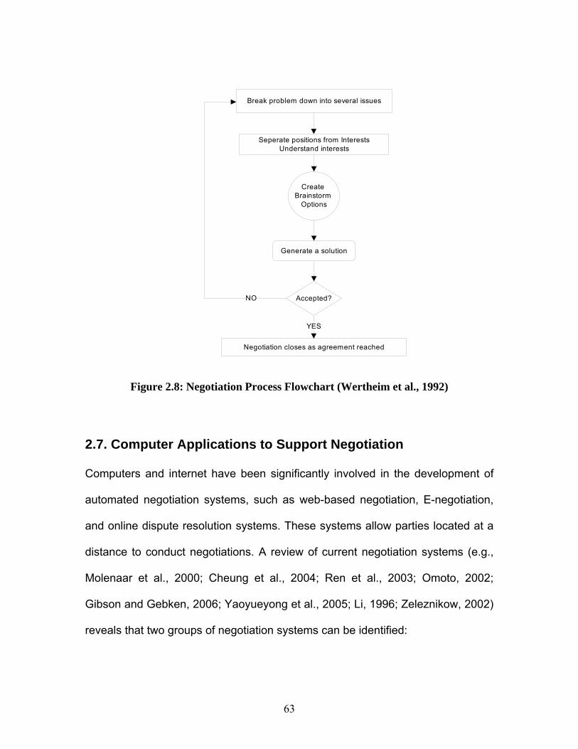
63
Break problem down into several issues
Seperate positions from Interests Understand interests
Create Brainstorm
Options
Generate a solution
Accepted?
Negotiation closes as agreement reached
NO
YES
Figure 2.8: Negotiation Process Flowchart (Wertheim et al., 1992)
2.7. Computer Applications to Support Negotiation
Computers and internet have been significantly involved in the development of
automated negotiation systems, such as web-based negotiation, E-negotiation,
and online dispute resolution systems. These systems allow parties located at a
distance to conduct negotiations. A review of current negotiation systems (e.g.,
Molenaar et al., 2000; Cheung et al., 2004; Ren et al., 2003; Omoto, 2002;
Gibson and Gebken, 2006; Yaoyueyong et al., 2005; Li, 1996; Zeleznikow, 2002)
reveals that two groups of negotiation systems can be identified:
64
1) Early Negotiation Support Systems (NSSs), which have been
restricted to informing parties about past rounds of negotiation,
parties, preferences, and the progress of current negotiation; and
2) Recently-developed Negotiation Decision Support Systems
(NDSSs), which have the advantage of incorporating decision-
making aspects into negotiation support systems to help decision
makers arrive at better negotiation outcomes. They help decision
makers overcome the challenges of conventional negotiation
through a range of analytical tools that can clarify interests, identify
tradeoffs, recognize party satisfaction, and generate optimal
solutions (Thiessen and McMahon, 2000). Their aim is to better
prepare decision makers for negotiation or to support them during
the negotiation process.
2.7.1. Review of Existing Negotiation Support Systems
There have been many research efforts conducted in the area of negotiation
support systems due to their important role in facilitating dispute resolution in
different communities. The developed negotiation support systems are proposed
for resolving disputes in various industries such as manufacturing, financial, and
Information Technology (IT). There are also a few negotiation support system
developed for resolving family disputes which have different characteristics than
of those disputes in the construction industry. The reviewed studies are
summarized in Table 2.8.
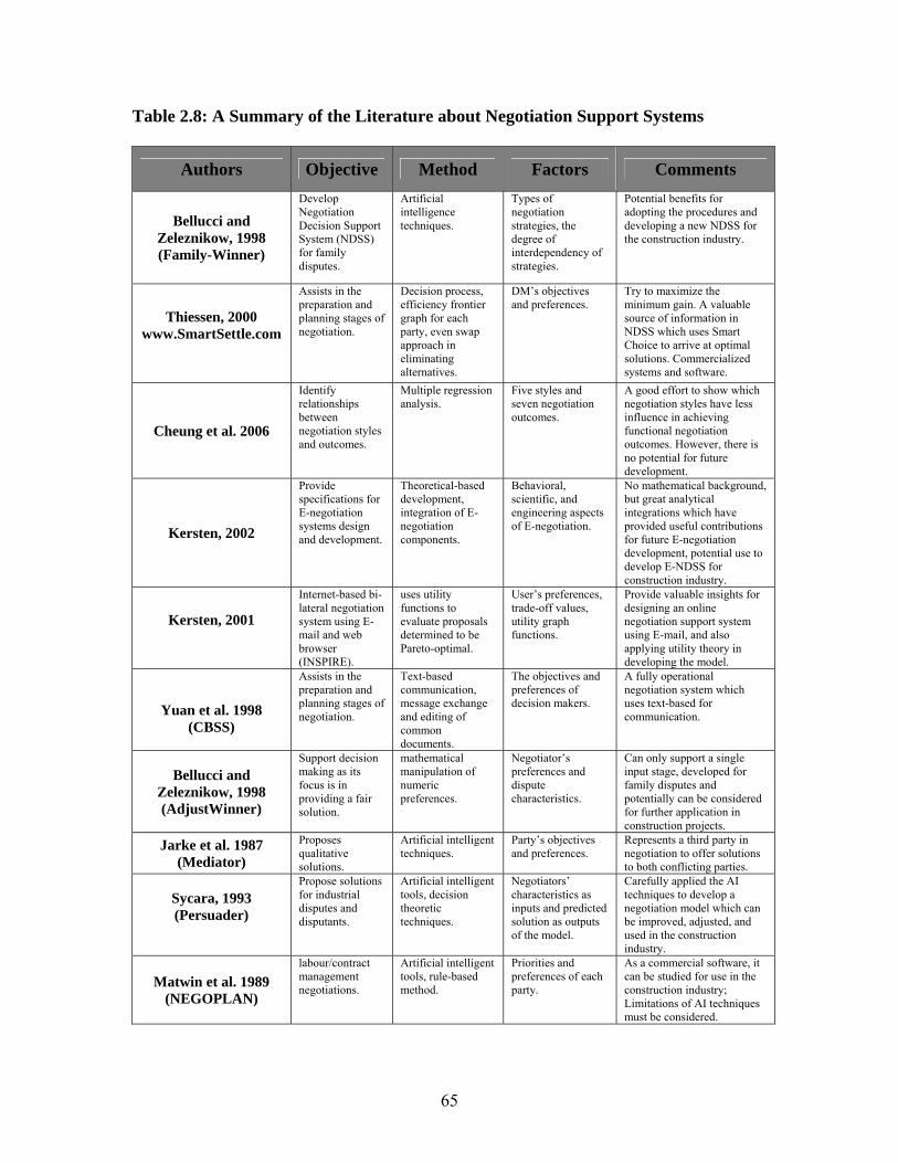
65
Table 2.8: A Summary of the Literature about Negotiation Support Systems
Authors Objective Method Factors Comments
Bellucci and Zeleznikow, 1998 (Family-Winner)
Develop Negotiation Decision Support System (NDSS) for family disputes.
Artificial intelligence techniques.
Types of negotiation strategies, the degree of interdependency of strategies.
Potential benefits for adopting the procedures and developing a new NDSS for the construction industry.
Thiessen, 2000 www.SmartSettle.com
Assists in the preparation and planning stages of negotiation.
Decision process, efficiency frontier graph for each party, even swap approach in eliminating alternatives.
DM’s objectives and preferences.
Try to maximize the minimum gain. A valuable source of information in NDSS which uses Smart Choice to arrive at optimal solutions. Commercialized systems and software.
Cheung et al. 2006
Identify relationships between negotiation styles and outcomes.
Multiple regression analysis.
Five styles and seven negotiation outcomes.
A good effort to show which negotiation styles have less influence in achieving functional negotiation outcomes. However, there is no potential for future development.
Kersten, 2002
Provide specifications for E-negotiation systems design and development.
Theoretical-based development, integration of E-negotiation components.
Behavioral, scientific, and engineering aspects of E-negotiation.
No mathematical background, but great analytical integrations which have provided useful contributions for future E-negotiation development, potential use to develop E-NDSS for construction industry.
Kersten, 2001
Internet-based bi-lateral negotiation system using E-mail and web browser (INSPIRE).
uses utility functions to evaluate proposals determined to be Pareto-optimal.
User’s preferences, trade-off values, utility graph functions.
Provide valuable insights for designing an online negotiation support system using E-mail, and also applying utility theory in developing the model.
Yuan et al. 1998
(CBSS)
Assists in the preparation and planning stages of negotiation.
Text-based communication, message exchange and editing of common documents.
The objectives and preferences of decision makers.
A fully operational negotiation system which uses text-based for communication.
Bellucci and Zeleznikow, 1998 (AdjustWinner)
Support decision making as its focus is in providing a fair solution.
mathematical manipulation of numeric preferences.
Negotiator’s preferences and dispute characteristics.
Can only support a single input stage, developed for family disputes and potentially can be considered for further application in construction projects.
Jarke et al. 1987 (Mediator)
Proposes qualitative solutions.
Artificial intelligent techniques.
Party’s objectives and preferences.
Represents a third party in negotiation to offer solutions to both conflicting parties.
Sycara, 1993 (Persuader)
Propose solutions for industrial disputes and disputants.
Artificial intelligent tools, decision theoretic techniques.
Negotiators’ characteristics as inputs and predicted solution as outputs of the model.
Carefully applied the AI techniques to develop a negotiation model which can be improved, adjusted, and used in the construction industry.
Matwin et al. 1989 (NEGOPLAN)
labour/contract management negotiations.
Artificial intelligent tools, rule-based method.
Priorities and preferences of each party.
As a commercial software, it can be studied for use in the construction industry; Limitations of AI techniques must be considered.

66
2.8. Summary
In this chapter, conflict-resolution and decision-making systems and models are
reviewed and the concepts, theories, requirements, constraints, methodologies,
and techniques in the modeling of decision-making processes were extensively
discussed. Conflicts and causes of disputes in construction were briefly
explained, and various dispute resolution methods (e.g., arbitration, negotiation,
mediation) were presented. Negotiation was presented as the most preferred
method for construction participants due to its low cost and low hostility as well
as the fact that it provides the parties with more control over their options and
outcomes. Group decision-making approaches, such as game theory and
negotiation analysis, were explained, and negotiation decision support systems
were listed and the characteristics of each system were summarized.
The contents of this chapter will be used and addressed in the development of a
negotiation methodology for construction disputes proposed in Chapters 4, 5, 6,
and 7. The proposed methodology takes into account the attitudes of negotiators
and combines the strategic level of decision analysis with the tactical level of
negotiation outcomes. Chapter 3 presents the Graph Model for Conflict
Resolution (GMCR) and overviews its modeling and analysis stages. GMCR is
used to develop the strategic level of attitude-based negotiation methodology
proposed in Chapters 4 and 5.
67
CHAPTER 3 Graph Model for Conflict Resolution
3.1. Introduction
Finding suitable tools for resolving social and environmental disputes such as
brownfield disputes is the objective of many researchers worldwide. They have
developed many formal modeling techniques and methodologies for
systematically studying conflicts that have two or more decision makers, each of
whom can have multiple objectives and interests. In particular, the Graph Model
for Conflict Resolution (GMCR) (Fang et al., 1993) is a methodology for modeling
and analyzing decision makers’ interactions in a conflict in order to find stable
states for all decision makers (DMs) which represent feasible resolutions of the
conflict at the strategic level. GMCR was originated from conflict analysis (Fraser
and Hipel, 1984) which in turn is an expansion of metagame theory (Howard,
1971). The Graph Model utilizes concepts and definitions from graph theory, set
theory, and game theory. Each DM’s possible moves from one state to other
states are captured using a directed graph in which nodes represent states and
arcs indicate state transitions controlled by the DM (Hipel et al., 1999). A state is
a potential outcome, or scenario, of the conflict. It should be mentioned that most
of the contents of this Chapter are taken from Fraser and Hipel (1984), Hipel
(2005, 2008 a, b), and Fang et al. (1993).
68
The associated decision support system GMCR II conveniently implements the
Graph Model for conflict resolution and provides speedy, cost-efficient, and
accurate advice for the DMs involved in conflict resolution process (Fang et al.,
2003a and b). It incorporates the option form for conflict modeling and
determines the stability of every state for each DM under a broad range of
stability types (Hipel et al., 1997). GMCR II is generally able to predict a variety of
equilibrium information, which enhances the analyst’s understanding of the
conflict and results in useful advice to DMs about whether possible outcomes are
strategically stable.
3.2. GMCR Overview
The systematic procedure for applying the Graph Model follows two main stages:
modeling and analyzing, as shown in Figure 3.1. In the modeling stage, the
problem is structured by determining the DMs, the states, the possible state
transitions controlled by each DM, and each DM’s relative preferences with
respect to the states. In the analysis stage, the stability of each state from each
DM’s viewpoint is determined. The objective is to find some stable states that
represent a resolution of the conflict. The essential parts of a graph model in
option form are the DMs and the options available to each DM. In general, a DM
may exercise any combination of the options he or she controls to create a
strategy. When every DM has selected a strategy, a state is defined.
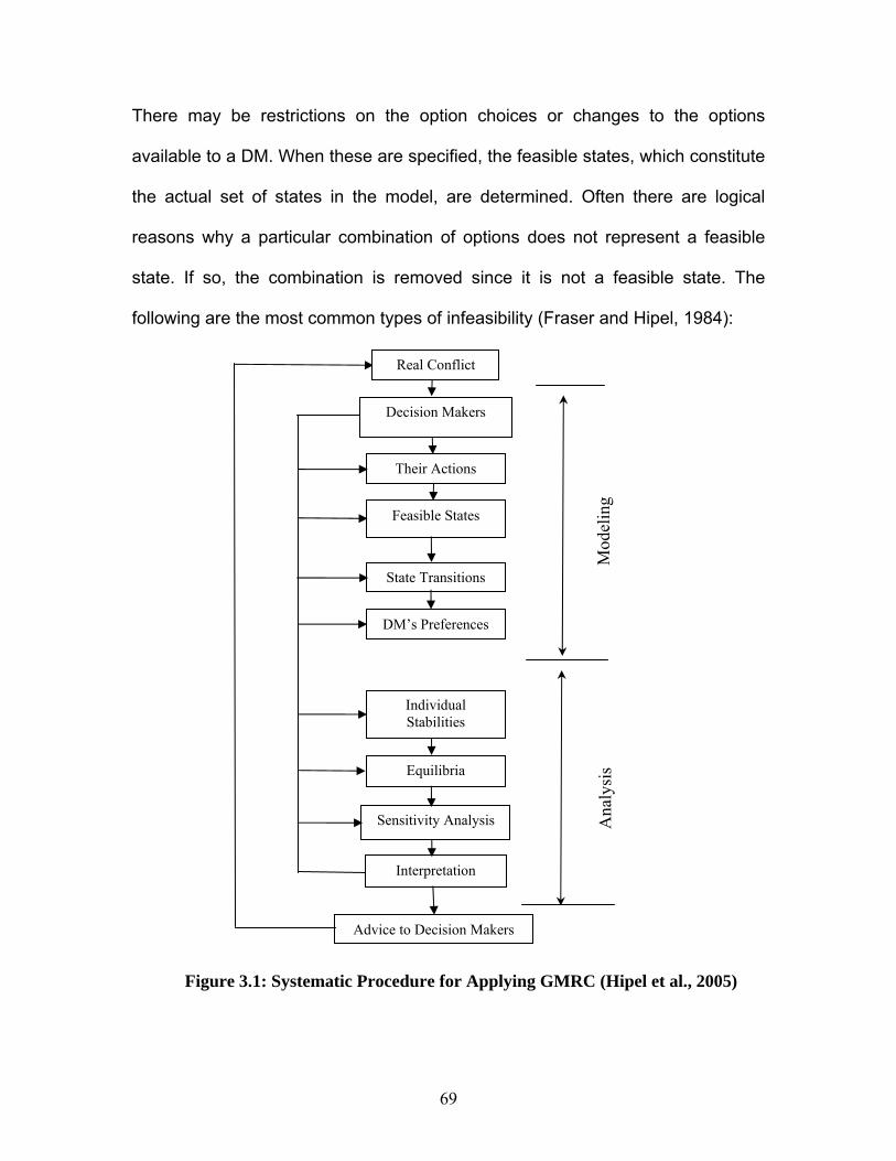
69
There may be restrictions on the option choices or changes to the options
available to a DM. When these are specified, the feasible states, which constitute
the actual set of states in the model, are determined. Often there are logical
reasons why a particular combination of options does not represent a feasible
state. If so, the combination is removed since it is not a feasible state. The
following are the most common types of infeasibility (Fraser and Hipel, 1984):
Advice to Decision Makers
Their Actions
Feasible States
State Transitions
DM’s Preferences
Individual Stabilities
Real Conflict
Sensitivity Analysis
Equilibria
Interpretation
Ana
lysi
s
Decision Makers
Mod
elin
g
Figure 3.1: Systematic Procedure for Applying GMRC (Hipel et al., 2005)
70
1. The availability of an option depends on the selection of another option.
For example, option “A” can be selected only if option “B” is selected;
2. An option must be taken when another option is taken (i.e., “A” must be
taken when “B” is taken, and “A” cannot be taken when “B” is not taken);
3. From a group of options, at least one must be taken; and
4. From a group of options, only one can be taken (mutually exclusive). For
instance, option “A” or option “B” or neither can be chosen, but not both.
The state-to-state transitions controlled by a DM are exactly those implied by a
unilateral change in the DM’s option selection. These steps produce the usual set
of directed graphs, and the graph model is completed by the incorporation of
each DM’s relative preferences among the feasible states. Since each DM’s
graph has the same set of nodes, it is often useful to show all DMs’ graphs on
the same diagram by simply combining them as a single graph and labelling
each arc to indicate the DM who controls it. Such a graph is referred to as the
integrated graph of the model.
The Graph Model can handle both transitive and intransitive preferences.
However, in most real-life conflicts, a DMs’ preferences can be assumed to be
transitive and thus expressed as a ranking (ordering) of the states from most to
least preferred, in which ties are allowed. Some of the advantages of applying a
graph model compared with the classical normal form (Von Neumann and
Morgenstern, 1944) include the following: 1) the graph model can handle

71
irreversible moves; 2) it provides a flexible framework for defining, comparing,
and characterizing solution concepts; and 3) it can be applied easily in practice.
In GMCR, the set of all states that DM i can unilaterally reach from state s in one
step is the reachable list (R). A Unilateral Improvement (UI) from a particular
state for a specific DM is a more preferred state (for that DM) to which he or she
can unilaterally move in one step. It follows that R can be partitioned into three
subsets: 1) the set of unilateral improvements from state s for DM i, the set of
unilateral disimprovements from state s for DM i, and the unilateral changes to
equally preferred states.
3.3. Stability Analysis
The stability of states for DMs is defined by various solution concepts, or stability
definitions as listed in Table 3.1. Nash stability (Nash, 1950, 1951) reflects a DM
who thinks only one step ahead. In general metarationality (GMR) (Howard,
1971) and sequential stability (SEQ) (Fraser and Hipel, 1984), a DM considers
exactly two steps ahead, whereas in symmetric metarationality (SMR) (Howard,
1971), the DM takes into account three steps by assessing available escapes
from any sanctions that may be imposed by the opponents. A disimprovement
refers to the tendency of a DM to move to a less preferred state in order to reach
a more preferred state eventually, or to block the unilateral improvements of
other DMs. In both Nash and sequential stabilities, disimprovements are never
permitted, while in general and symmetric metarationality only disimprovements
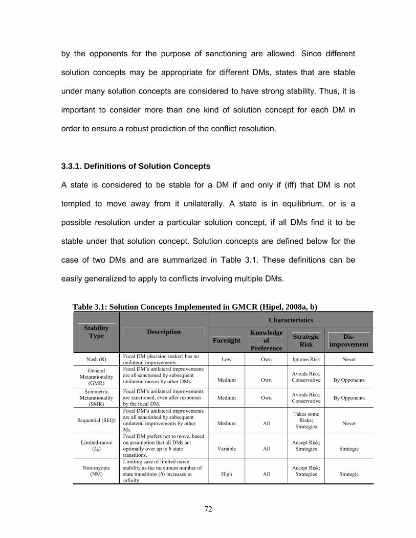
72
by the opponents for the purpose of sanctioning are allowed. Since different
solution concepts may be appropriate for different DMs, states that are stable
under many solution concepts are considered to have strong stability. Thus, it is
important to consider more than one kind of solution concept for each DM in
order to ensure a robust prediction of the conflict resolution.
3.3.1. Definitions of Solution Concepts
A state is considered to be stable for a DM if and only if (iff) that DM is not
tempted to move away from it unilaterally. A state is in equilibrium, or is a
possible resolution under a particular solution concept, if all DMs find it to be
stable under that solution concept. Solution concepts are defined below for the
case of two DMs and are summarized in Table 3.1. These definitions can be
easily generalized to apply to conflicts involving multiple DMs.
Table 3.1: Solution Concepts Implemented in GMCR (Hipel, 2008a, b)
Characteristics Stability
Type Description Foresight
Knowledge of
Preference
Strategic Risk
Dis-improvement
Nash (R) Focal DM (decision maker) has no unilateral improvements. Low Own Ignores Risk Never
General Metarationality
(GMR)
Focal DM’s unilateral improvements are all sanctioned by subsequent unilateral moves by other DMs.
Medium
Own
Avoids Risk; Conservative
By Opponents
Symmetric Metarationality
(SMR)
Focal DM’s unilateral improvements are sanctioned, even after responses by the focal DM.
Medium Own Avoids Risk; Conservative By Opponents
Sequential (SEQ)
Focal DM’s unilateral improvements are all sanctioned by subsequent unilateral improvements by other Ms.
Medium
All
Takes some Risks;
Strategies
Never
Limited-move (Lh)
Focal DM prefers not to move, based on assumption that all DMs act optimally over up to h state transitions.
Variable
All
Accept Risk; Strategies
Strategic
Non-myopic (NM)
Limiting case of limited move stability as the maximum number of state transitions (h) increases to infinity.
High
All
Accept Risk; Strategies
Strategic

73
1. Nash stability: Under the Nash solution concept, a DM will move to a
more preferred state whenever possible, regardless of any possible
countermoves by the opponent. Hence, a state s is Nash stable for DM i iff
i has no unilateral improvements from s.
2. General metarationality (GMR): A state s is general metarational stable
for DM i iff for every UI i can take advantage of, the opponent, DM j, can
subsequently move to a state that is at most as good for i as the original
state s. In other words, DM j can sanction each of i’s UIs by moving to a
state that is less than or equally preferred to state s by DM i. Therefore, a
DM who follows general metarationality selects his or her unilateral moves
in light of the opponent’s possible reactions, irrespective of the opponent’s
preferences.
3. Symmetric metarationality (SMR): A state s is symmetric metarational
stable for DM i iff not only every UI for i from s is sanctioned by the
opponent, but also no unilateral counter-reply by DM i can leave it better
off than the original state s. It is noted that the above solution concepts are
used only for rational or regular stability analysis.
4. Sequential stability (SEQ): A state s is sequentially stable for DM i iff
every UI for i from s is credibly sanctioned by the sanctioner DM j. A
credible sanction is a sanction that directly benefits the sanctioner. In
other words, the second possible movement is a UI for the sanctioner. A
DM who follows sequential stability takes into consideration not only his or
her own possible moves, but also the opponent’s unilateral improvements.

74
When the above solution concepts are used within the paradigm of GMCR it is
important to consider the relationship between the proposed solution concepts
and the stability of states so that different equilibrium states can be reached. The
following theorems are taken into account to determine the stability of a state:
Theorem 1 (Fang et al., 1993): For i є N and c є C, if c є NashiC , then c є
SMRiC ; if c
є SMRiC , then c є
GMRiC . Theorem 2 (Fang et al., 1993): For i є N and c є C, if c є
CNash i , then c є CSEQ i ; if c є CSEQ i , then c є CGMR i . Then, a state is
said to be an equilibrium state for Nash stability, general metarationality,
symmetric metarationality and sequential stability, if and only if it is Nash stable,
generally metarational, symmetrically metarational, and sequentially stable for all
DMs, respectively.
3.4. Sensitivity Analyses
Sensitivity analysis is used to make sure that uncertainty in the DMs’ preferences
and other model preferences, as well as sudden or unforeseen events cannot
affect the robustness of the stability analyses. A sensitivity analysis focuses on
the implications of changes in model parameters, by considering, for example,
how the preferences of a DM would have to be changed in order to produce
more preferable equilibria for another DM. A reasonable range of possible
preferences can be analyzed in order to ascertain how equilibria are affected. If
the equilibria do not change as preferences are modified, one can have greater
confidence in the results of the analysis. Alternatively, when small preference
changes produce dramatic equilibria changes, then the analyst must ensure that
75
the model is as accurate and reliable as possible. The following are types of
sensitivity analyses:
• Preference changes,
• Option modification or expansion,
• Other decision makers added into the game,
• Consideration of other kinds of human behaviour and attitudes (different
solution concepts), and
• Consideration of coalitions.
3.5. Summary
In this chapter, Graph Model for Conflict Resolution was presented and its
methodology and involving stages were reviewed. The Graph Model is a
promising methodology to model complex conflicts and provide the involved
decision makers with potential resolutions at strategic level. Therefore, the Graph
Model approach is first improved in Chapter 4 to incorporate the attitudes of
decision makers into the Graph Model methodology. Subsequently, the proposed
attitude-based Graph Model is utilized to develop an attitude-based negotiation
methodology at the strategic level for resolving complex disputes in construction
operations. The strategic negotiation methodology proposed in Chapters 4 and 5,
will be complemented by a tactical negotiation methodology proposed in
Chapters 6 and 7 for two and multiple decision makers, respectively.
76
CHAPTER 4 Attitude-Based Strategic Negotiation Methodology Involving Two Decision Makers
4.1. Introduction
The primary objective of this chapter is to propose an attitude-based strategic
negotiation methodology for resolving complex construction disputes using the
Graph Model for Conflict Resolution (GMCR) technique. Because controversies
and differences of opinion and attitudes are so pervasive in human decision
making, there is a great need for flexible decision technologies to assist in the
understanding, modeling, analyzing, and managing of strategic conflicts. The
need for such decision methodologies is intensified when human factors, such as
attitudes, are added to the consideration of conflict analysis.
This chapter focuses on the strategic level of negotiation, which defines a set of
the most beneficial decision options that can be further negotiated at a tactical
level discussed in Chapters 6 and 7. This chapter first introduces the proposed
negotiation framework for construction disputes. To provide an understanding of
construction negotiations, the characteristics of negotiations in construction
projects are identified, and the behavior of the parties involved in negotiations is
discussed. Attitude-based solution concepts for conflicts in construction projects
are then formally defined, and the performance of the proposed attitude-based
stability analyses within the paradigm of GMCR is described. The proposed
77
strategic negotiation methodology is systematically developed using a brownfield
construction case study in order to clarify the advantages and capabilities of the
methodology. Finally, the resulting strategic decision options provided by the
methodology are discussed.
4.2. Proposed Negotiation Framework
The proposed negotiation framework consists of three major components which
constitute three major stapes (i.e., objectives): 1) understand construction
negotiations, 2) develop negotiation methodology, and 3) design a negotiation
decision support system. These three components conveniently constitute a
systematic negotiation model that consider the strategic as well as the tactical
levels of decision making. Each component of the framework also encompasses
key subcomponents. A diagram of the proposed negotiation framework is
provided in Figure 4.1. This chapter addresses the first component of the
proposed framework, as well as the strategic level defined within the second
component when only two decision makers (DMs) are involved in the negotiation
process.
4.3. Understand Construction Negotiations
Generally, if a negotiation model is to be developed for a specific purpose, it is
vital to understand the nature and the characteristics of the problem at hand. To
this end, an extensive literature review was carried out in Chapter 2, relevant
case study data were obtained, and several meetings were held with construction

78
professionals and participants at Kitchener City Hall. These meetings were useful
in a practical sense to identify the key issues involved in construction
negotiations, particularly when the municipality is a key DM in a construction
conflict. Negotiations in the construction industry are normally studied from three
perspectives: the characteristics of construction negotiations (e.g., parties
involved, types and number of conflicting issues, and project types), the
characteristics of the negotiators (e.g., attitudes, positions, and choices), and the
inherent challenges and needs of the decision making. These perspectives are
explained in the following subsections.
UnderstandConstruction Negotiation
UnderstandConstruction Negotiation
Develop NegotiationMethodology
Develop NegotiationMethodology
Design Negotiation
Decision Support System
Design Negotiation
Decision Support System
NegotiationCharacteristics
Negotiators’Characteristics
ChallengesAnd Needs
Methodology
Implementation
Design Components
Verification
Test
(Case Study)
IssuesIssues
DMs & OptionsDMs & Options
Attitude-BasedUtility
Functions
Attitude-BasedUtility
Functions
Attitude-BasedGMCR
Attitude-BasedGMCR
StrategicDecision
StrategicDecision
StrategicLevel
StrategicLevel
DetailedResolution
DetailedResolution
TacticalLevel
TacticalLevel
Figure 4.1: Proposed Negotiation Framework
2
3
5
6
1
4
4

79
4.3.1. General Negotiation Characteristics
With respect to negotiations for resolving construction disputes, the following
characteristics reflect the series of factors construction participants consider
when negotiations take place (Pena-Mora and Wang, 1998):
A) Domain-dependent knowledge: Participants in construction operations are
normally experts in only one domain of knowledge and, as such, often know little
about other domains. For example, architects are experts in the aesthetics of
structures whereas engineers have experience in the design and analysis of
structures. Each group views a project from its own perspective. Therefore, none
of the involved participants has an in-depth global view of all knowledge domains
(Odeh and Battaineh, 2002). The unfamiliarity with other knowledge domains
within projects can cause disagreement when conflicts arise and may hinder the
finding of a common meeting ground for the participants.
B) Competitive-cooperative environment: In the construction industry, disputes
are dealt with according to the objectives of the project and the participants. The
participants (rationally) have the common goal of successful project completion
because it ensures a profit for all. If the project fails, some or all of them will lose
because not only will they not profit from the project but they will also be liable for
its failure. Consequently, they are willing to cooperate with each other in order to
finish the project on time and within the budget (Hegazy, 2002). At the same
time, they will also try to maximize their own profits at the expense of the other

80
parties, thus departing from the cooperative nature of the construction team. This
competitive-cooperative environment has an impact on the participants’
strategies and, subsequently, on the outcomes of the negotiation.
C) Strategy-influenced outcome: Because of the competitive-cooperative nature
of construction work, the DMs involved try to maximize their gain without losing
cooperation (Fellow et al., 1994). They take a course of action (called a strategy)
that influences the outcome of the negotiations. Since a competitive-cooperative
condition exists throughout the project’s life cycle, these strategies are employed
frequently and have a strong influence on the outcome of negotiations. The most
common strategy and the one most easily used by participants is domain-
dependent knowledge. Participants can influence the outcome of the issues
related to their specialty by exaggerating their contributions without being held
fully accountable because others are not fully familiar with the issues. This
domain-dependent barrier can prevent participants from fully realizing the
situation that any other participant faces. Bringing in an expert in a given area to
inform teams who are unfamiliar with the issues can prevent the use of this
strategy. However, the complexity of the problem increases as more people
become involved in the negotiations and their preferences must also be
considered. Therefore, given the competitive-cooperative nature and the
prevalence of domain-dependent barriers, using a manipulative strategy is
common in construction particularly when the involved DMs have aggressive
behavior and negative attitudes toward one another (Walton et al., 2000).

81
4.3.2. Negotiators’ Characteristics
The participation of people in the construction industry, such as the owner, the
government, the contractor, and the stakeholders, depends on their position.
When conflicts and disputes arise, the DMs involved use different strategies to
maximize their benefits during the negotiation process (Essex, 1996). The DMs
involved in construction projects will certainly have different attitudes about
different projects and will try to prioritize the conflicting issues that are common in
projects (Heng, 1996). For example, the two main conflicting issues between the
owner and the contractor are usually time extensions and cost overruns, and
both DMs know their own advantages and disadvantages with respect to these
issues. The contractor knows his costs exactly, can adjust prices for the
maximum revenue, and can accept or reject a settlement. The owner, on the
other hand, has a strong advantage in that he owns the project and controls the
money. The owner is, however, bound by the procurement rules, regulations, and
approvals put in place by the government. The contractor has a larger degree of
freedom in making his proposal and accepting a settlement and thus, he has the
advantage of setting the pace and direction of the negotiation (Levin, 1998).
4.3.3. Challenges and Needs
The construction industry is facing increasing challenges due to the growing
complexity of the design, construction, operation, and maintenance stages. Such
complexities boost the level and the number of risks and uncertainties involved in
construction operations. Moreover, construction projects are often behind

82
schedule or have cost overruns and the DMs involved prefer to blame other DMs
for construction delays (Hegazy, 2002; Glasner, 2000). These challenges can
increase the possibility of conflict among participants and also influence the
decision-making process, particularly with respect to conflict negotiation.
Construction negotiations are more challenging because the participants lack
negotiation skills and they belong to different knowledge-dependent domains
(Mnookin et al., 2000). These challenges can significantly hinder the progress of
construction projects, and they must therefore be appropriately addressed in any
effective decision-making methodology. Models that address these challenges
will better mimic the societal activities of those participating in conflict resolution.
Table 4.1 summarizes discussions in Subsections 4.3.1, 4.3.2, and 4.3.3 with
respect to a brownfield reconstruction case study. Table 4.1 points out the
characteristics of the parties involved in a brownfield redevelopment project when
they intend to negotiate conflicting issues, such as redevelopment costs. These
characteristics have been compiled based on previous studies (e.g.,
Stipanowich, 1997; Fellow et al., 1994; Odeh and Battaineh, 2002) and several
meetings with the consultants, researchers, and representatives of the City of
Kitchener, located in southern Ontario, Canada, who are concerned with
Kitchener’s brownfield sites. It should be noted that the types and number of
parties involved in a construction project depend on the type of project. Although
contractors are often involved in negotiations in many situations, such as in
brownfield projects, initial negotiations normally take place between the current

83
property owner and the government; the contractor may be hired later. In the
brownfield case study used in this chapter, it is assumed that the two DMs
involved are the current property owner and the government, who are both
directly concerned about the costs and duration of the project. In future research,
a purchaser may be included later in the process. This case study will be also
used to systematically develop the proposed negotiation methodology as
explained in the following sections.
Table 4.1: Negotiators’ Characteristics in Brownfield Reconstruction
Party Characteristics
Owner
• Lack of funds or the will to cleanup the contaminated property, • Expects government help in marketing the land, • Wants to share its liabilities for cleanup through negotiation, • Sometimes refuses to cooperate when the owner must clean the land, • Avoids revealing his or her identity, • Tries to understand the concerns of the perspective purchaser, • Very concerned about the costs of redevelopment, and • Not concerned about the future risk of site contamination.
Purchaser
• Prefers to have environmental testing and certificate, • Wants to receive incentives from other parties, • Takes into account the preferences and interests of the owner, • Considers other options for investments, • Very concerned about the risks of buying the property, • Usually one purchaser is considered in buying the contaminated property, and • Considers time and cost of redevelopment and responsibilities of future
contamination not caused by purchaser.
Government
• Provides available resources of municipalities to make a deal among parties, • Has fair working relationship with both the owner and the purchaser, • Plays key role to initiate negotiation process in various phases, • Provides inducements for both the owner and the purchaser, • Wants to have contaminated property cleaned and redeveloped, • Considers private-owned brownfield sites as being different from public-owned
brownfield sites, • Uses reactive approach to deal with brownfield problems, • Has concerns about the justification of the resources used for brownfield
redevelopment, • Tends to be more risk averse, and • Non-remedied contamination is his key future concern.
84
4.4. Attitude-Based GMCR
Based on the previously discussed characteristics of construction negotiations,
the development of the proposed negotiation methodology involving only two
DMs at the strategic level is described in the remainder of this chapter, while the
development of the proposed methodology involving two DMs at the tactical
level, which complements that at the strategic level, is explained in Chapter 6.
At the strategic level, the proposed methodology uses the Graph Model for
Conflict Resolution, (GMCR) with its powerful modeling and stability analysis
stages. GMCR (Fang et al., 1993) is a comprehensive systems engineering
technique that provides strategic advice to a negotiator through a prescription for
actions that will achieve his or her preferred outcome. It also suggests to a
mediator which possible resolutions of the conflict would be stable and reveals to
a policymaker how the strategic structure of the situation shapes the outcome.
This strategic advice reflects the capacity of GMCR to identify individually stable
states and equilibria. It should be noted that GMCR is intended to be used
prescriptively to advise a negotiator in a negotiation round rather than
descriptively or normatively to predict which choices will be made or to determine
which choices “should” be made (Kilgour, 2007).
4.4.1. GMCR Formal Definition
Formal definition of Graph Model for Conflict Resolution (GMCR): A graph model
of a conflict is a 4-tuple (N, C, (Si)i є N , (≥i) i є N ). N is the set of all (DMs). C is the
85
set of all states of the focal decision making situation, where |C| ≥ 2. For i є N , Si
is a function from C to the power set P(C) of C such that c ∉ Si(c) є P(C) for all c
є C. Si is called the irreflexive reachable list function of DM i є N and Si(c) is
called the irreflexive reachable list of DM i є N from c є C. ≥i is the preference of
DM i є N on C. Defining Ei as the set {(c, c' ) є C × C | c' є Si(c)}, there is the
graph (C, Ei) of DM i є N, denoted by Gi, where C is the set of all vertices of the
graph and Ei is the set of all arcs of the graph (Fang et al., 1993).
For i є N and c, c' є C, c ≥i c' means that c is more or equally preferred to c' by
DM i. c ~i c means that c ≥i c' and c' ≥i c, that is, c is equally preferred to c' by DM
i. c >i c' means that c ≥i c' and “not (c' ≥i c)” that is, c is strictly more preferred to c'
by DM i. DM i’s preferences ≥i is said to be transitive, if and only if for all c, c' , c"
є C, if c ≥i c' and c' ≥i c" then c ≥i c".≥i is said to be anti-symmetric, if and only if
for all c, c' є C, if c ≥i c' and c' ≥i c then c = c' . ≥i is said to be complete, if and
only if for all c, c' є C, c ≥i c' or c' ≥i c (Fang et al., 1993).
4.4.2. Attitude Representation
In construction conflicts and disputes, the attitudes of construction participants
can affect the outcome of their negotiations. Therefore, analyzing the conflict as
well as the accompanying attitudes of the DMs is useful for a better
understanding of the negotiation process. It is also beneficial to model DMs’
attitudes and incorporate them into construction negotiation methodology so that
the influence of DMs’ attitudes can be examined.
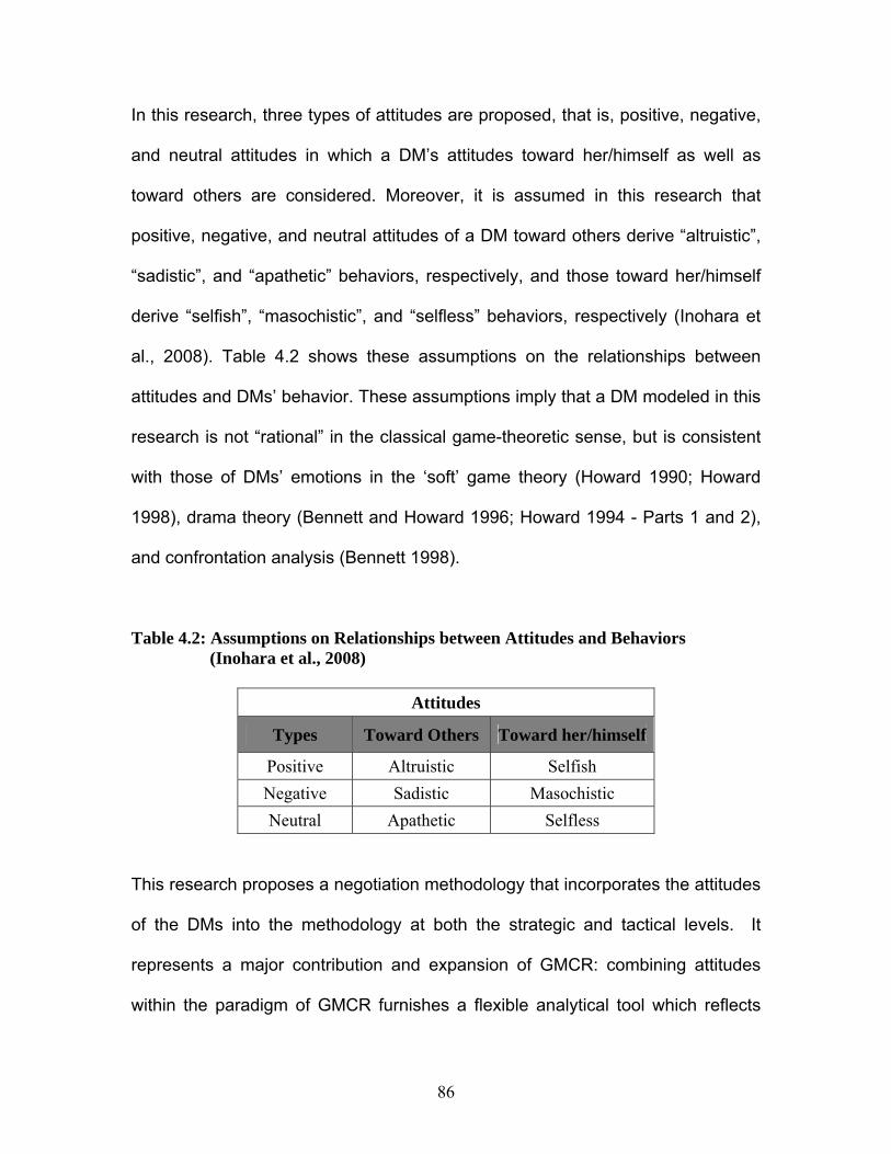
86
In this research, three types of attitudes are proposed, that is, positive, negative,
and neutral attitudes in which a DM’s attitudes toward her/himself as well as
toward others are considered. Moreover, it is assumed in this research that
positive, negative, and neutral attitudes of a DM toward others derive “altruistic”,
“sadistic”, and “apathetic” behaviors, respectively, and those toward her/himself
derive “selfish”, “masochistic”, and “selfless” behaviors, respectively (Inohara et
al., 2008). Table 4.2 shows these assumptions on the relationships between
attitudes and DMs’ behavior. These assumptions imply that a DM modeled in this
research is not “rational” in the classical game-theoretic sense, but is consistent
with those of DMs’ emotions in the ‘soft’ game theory (Howard 1990; Howard
1998), drama theory (Bennett and Howard 1996; Howard 1994 - Parts 1 and 2),
and confrontation analysis (Bennett 1998).
Table 4.2: Assumptions on Relationships between Attitudes and Behaviors (Inohara et al., 2008)
Attitudes
Types Toward Others Toward her/himself
Positive Altruistic Selfish Negative Sadistic Masochistic Neutral Apathetic Selfless
This research proposes a negotiation methodology that incorporates the attitudes
of the DMs into the methodology at both the strategic and tactical levels. It
represents a major contribution and expansion of GMCR: combining attitudes
within the paradigm of GMCR furnishes a flexible analytical tool which reflects

87
how the DMs’ attitudes may change the strategic outcomes of the negotiation.
The range of definitions for attitudes in this section follows those defined by
Inohara et al. (2007).
4.4.3. Formal Definition of Attitude
In this research, three basic types of attitude are defined and used to develop the
negotiation methodology. A DM’s attitude is defined toward him/helself as well as
toward other DMs involved in negotiation.
In order to formally define attitude, at least two decision makers “DM i” and “DM j”
should be considered. For DMs i, j є N, let Ei = {+, 0, –}N represent the set of
attitudes of DM i. An element ei є Ei is called the attitudes of DM i for which ei =
(eij) is the list of attitudes of DM i toward DM j for each j є N where eij є {+, 0, –}.
The eij is referred to as the attitude of DM i to DM j where the values eij = +, eij = 0
or eij = – indicates that DM i has a positive, neutral, or negative attitude toward
DM j, respectively.
According to the above definition, the attitudes of the DMs can be represented in
a matrix format, as shown in Table 4.3 in which each cell entry can take on a
Attitude Type
Positive (+) Neutral (0) Negative (-)
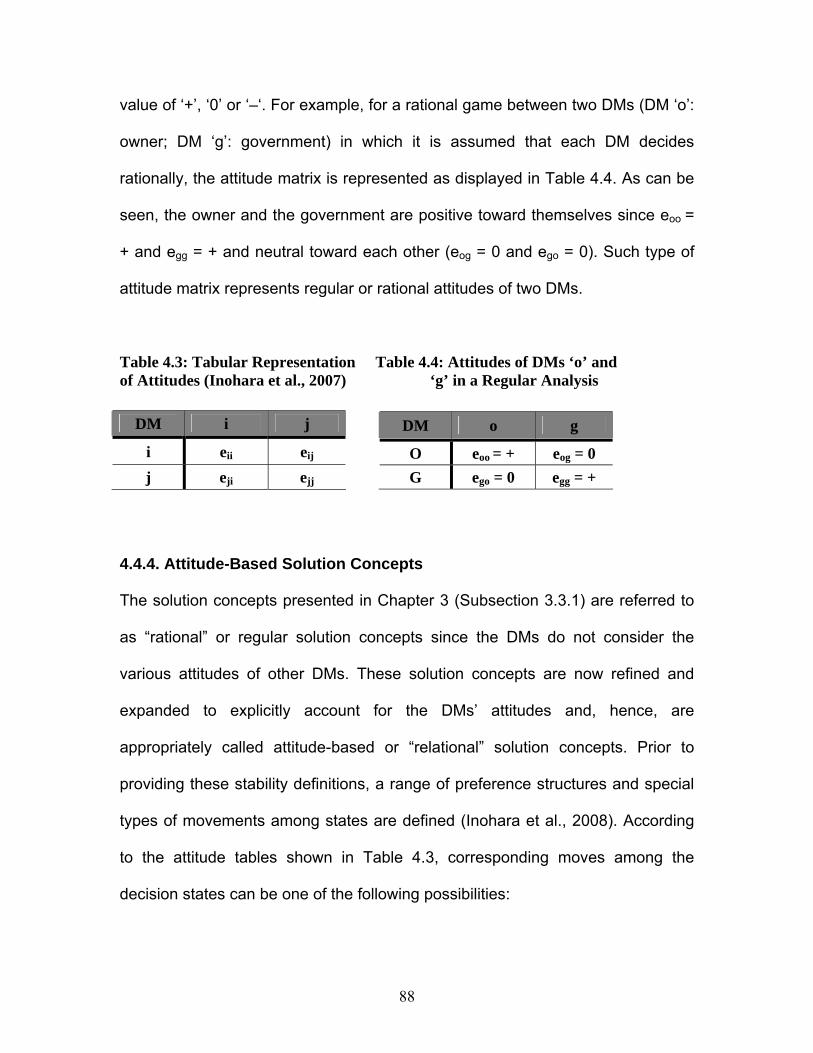
88
value of ‘+’, ‘0’ or ‘–‘. For example, for a rational game between two DMs (DM ‘o’:
owner; DM ‘g’: government) in which it is assumed that each DM decides
rationally, the attitude matrix is represented as displayed in Table 4.4. As can be
seen, the owner and the government are positive toward themselves since eoo =
+ and egg = + and neutral toward each other (eog = 0 and ego = 0). Such type of
attitude matrix represents regular or rational attitudes of two DMs.
Table 4.3: Tabular Representation Table 4.4: Attitudes of DMs ‘o’ and of Attitudes (Inohara et al., 2007) ‘g’ in a Regular Analysis
4.4.4. Attitude-Based Solution Concepts
The solution concepts presented in Chapter 3 (Subsection 3.3.1) are referred to
as “rational” or regular solution concepts since the DMs do not consider the
various attitudes of other DMs. These solution concepts are now refined and
expanded to explicitly account for the DMs’ attitudes and, hence, are
appropriately called attitude-based or “relational” solution concepts. Prior to
providing these stability definitions, a range of preference structures and special
types of movements among states are defined (Inohara et al., 2008). According
to the attitude tables shown in Table 4.3, corresponding moves among the
decision states can be one of the following possibilities:
DM o g
O eoo = + eog = 0 G ego = 0 egg = +
DM i j
i eii eij j eji ejj

89
Devoting Preference (Positive Attitude): The devoting preference (DP) of DM i є
N with respect to DM j є N is ≥j, denoted by DPij, such that for s, t є S, “s DPij t” if
and only if s ≥j t. In other words, the devoting preference means that if DM i has a
devoting preference for state s with respect to state t for DM j, then DM j must
prefer state s to state t. For example, if an owner has devoting preference or
positive attitudes toward a contractor in a construction negotiation, and the
contractor prefers state 2 to state 5, then the owner also prefers state 2 to state
5. A similar definition can be written for aggressive preference.
Aggressive Preference (Negative Attitude): The aggressive preference (AP) of
DM i є N with respect to DM j є N is NE(>j), denoted by APij, where NE(>j) is
defined as follows: for s, t є S, s NE(>j) t if and only if “s >j t” is not true. That is,
for s, t є S, s APij t if and only if s NE (>j) t (if and only if t ≥j s under completeness
of ≥j). In contrast to the devoting preference, the aggressive preference means
that if DM i has an aggressive preference for state s with respect to state t for DM
j, then DM j must prefer state t to state s. Using these concepts, as well as an
indifference preference represented by I, the relational preference can then be
determined. For example, if an owner has aggressive preference or negative
attitudes toward a contractor in a construction negotiation, and the contractor
prefers state 2 to state 5, then the owner must prefer state 5 to state 2.
Using these attitude-based possible moves, the following attitude-related terms
are defined and used in the stability analysis within the structure of GMCR:
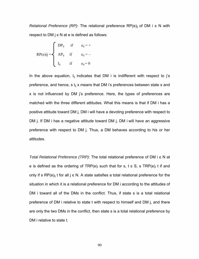
90
Relational Preference (RP): The relational preference RP(e)ij of DM i є N with
respect to DM j є N at e is defined as follows:
In the above equation, Iij indicates that DM i is indifferent with respect to j’s
preference, and hence, s Iij x means that DM i’s preferences between state s and
x is not influenced by DM j’s preference. Here, the types of preferences are
matched with the three different attitudes. What this means is that if DM i has a
positive attitude toward DM j, DM i will have a devoting preference with respect to
DM j. If DM i has a negative attitude toward DM j, DM i will have an aggressive
preference with respect to DM j. Thus, a DM behaves according to his or her
attitudes.
Total Relational Preference (TRP): The total relational preference of DM i є N at
e is defined as the ordering of TRP(e)i such that for s, t є S, s TRP(e)i t if and
only if s RP(e)ij t for all j є N. A state satisfies a total relational preference for the
situation in which it is a relational preference for DM i according to the attitudes of
DM i toward all of the DMs in the conflict. Thus, if state s is a total relational
preference of DM i relative to state t with respect to himself and DM j, and there
are only the two DMs in the conflict, then state s is a total relational preference by
DM i relative to state t.
DPij if eij = + APij if eij = – Iij if eij = 0
RP(e)ij =

91
Total Relational Reply (TRR): The total relational reply list of DM i є N at e for
state s є S is defined as the set {t є Ri(s) U {s} | t TRP(e)i s} ⊂ Ri(s) U {s},
denoted by TRR(e)i(s).
Relational less preferred or equally preferred states: RΦ(e)i (s) is the set of all
states which are “relationally less or equally preferred” to s by DM i (under
attitude e). It should be noted that NE(x TRP(e)i s) means that “x TRP(e)i s” is not
true. The same concept is defined for rational Φi (s).
It should be mentioned that the above attitude-based definitions are used in this
research for the first time to develop an attitude-based negotiation methodology
for resolving complex disputes among participants involved in the construction
industry. Employing the above proposed definitions, attitude-based solution
concepts can be defined as an extension of rational solution concepts when
attitudes are taken into account. Table 4.5 displays rational and attitude-based
solution concepts within the structure of GMCR. In Table 4.5, “N” is the set of
DMs, Ri(s) is the DM i’s reachable list, and R+i(s) is the DM i’s unilateral
improvement list. Attitude-based general metarationality (RGMR) is best
described as a situation in which a DM makes a unilateral move and opposing
DMs sanction that move with moves of their own. In RGMR, these sanctioning
moves do not have to be total attitude-based replies by the other DMs; they only
have to be possible moves by the sanctioning DMs. As in the case of RGMR, the
sanctioning moves need be only possible moves by the other DMs and do not
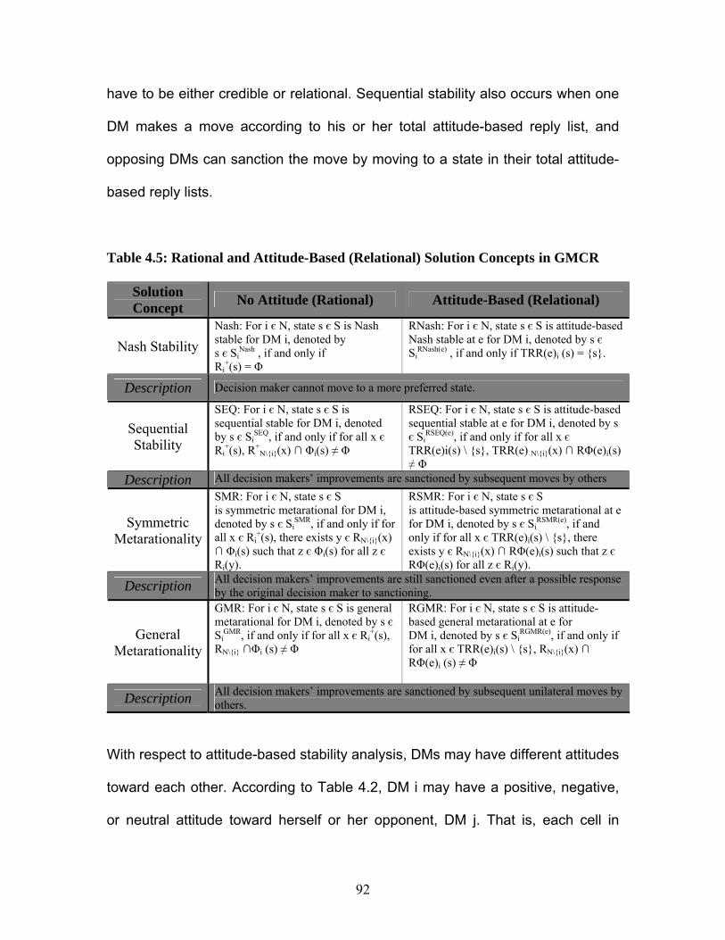
92
have to be either credible or relational. Sequential stability also occurs when one
DM makes a move according to his or her total attitude-based reply list, and
opposing DMs can sanction the move by moving to a state in their total attitude-
based reply lists.
Table 4.5: Rational and Attitude-Based (Relational) Solution Concepts in GMCR
Solution Concept No Attitude (Rational) Attitude-Based (Relational)
Nash Stability Nash: For i є N, state s є S is Nash stable for DM i, denoted by s є Si
Nash , if and only if Ri
+(s) = Φ
RNash: For i є N, state s є S is attitude-based Nash stable at e for DM i, denoted by s є Si
RNash(e) , if and only if TRR(e)i (s) = {s}.
Description Decision maker cannot move to a more preferred state.
Sequential Stability
SEQ: For i є N, state s є S is sequential stable for DM i, denoted by s є Si
SEQ, if and only if for all x є Ri
+(s), R+N\{i}(x) ∩ Φi(s) ≠ Φ
RSEQ: For i є N, state s є S is attitude-based sequential stable at e for DM i, denoted by s є Si
RSEQ(e), if and only if for all x є TRR(e)i(s) \ {s}, TRR(e) N\{i}(x) ∩ RΦ(e)i(s) ≠ Φ
Description All decision makers’ improvements are sanctioned by subsequent moves by others
Symmetric Metarationality
SMR: For i є N, state s є S is symmetric metarational for DM i, denoted by s є Si
SMR, if and only if for all x є Ri
+(s), there exists y є RN\{i}(x) ∩ Φi(s) such that z є Φi(s) for all z є Ri(y).
RSMR: For i є N, state s є S is attitude-based symmetric metarational at e for DM i, denoted by s є Si
RSMR(e), if and only if for all x є TRR(e)i(s) \ {s}, there exists y є RN\{i}(x) ∩ RΦ(e)i(s) such that z є RΦ(e)i(s) for all z є Ri(y).
Description All decision makers’ improvements are still sanctioned even after a possible response by the original decision maker to sanctioning.
General Metarationality
GMR: For i є N, state s є S is general metarational for DM i, denoted by s є Si
GMR, if and only if for all x є Ri+(s),
RN\{i} ∩Φi (s) ≠ Φ
RGMR: For i є N, state s є S is attitude-based general metarational at e for DM i, denoted by s є Si
RGMR(e), if and only if for all x є TRR(e)i(s) \ {s}, RN\{i}(x) ∩ RΦ(e)i (s) ≠ Φ
Description All decision makers’ improvements are sanctioned by subsequent unilateral moves by others.
With respect to attitude-based stability analysis, DMs may have different attitudes
toward each other. According to Table 4.2, DM i may have a positive, negative,
or neutral attitude toward herself or her opponent, DM j. That is, each cell in
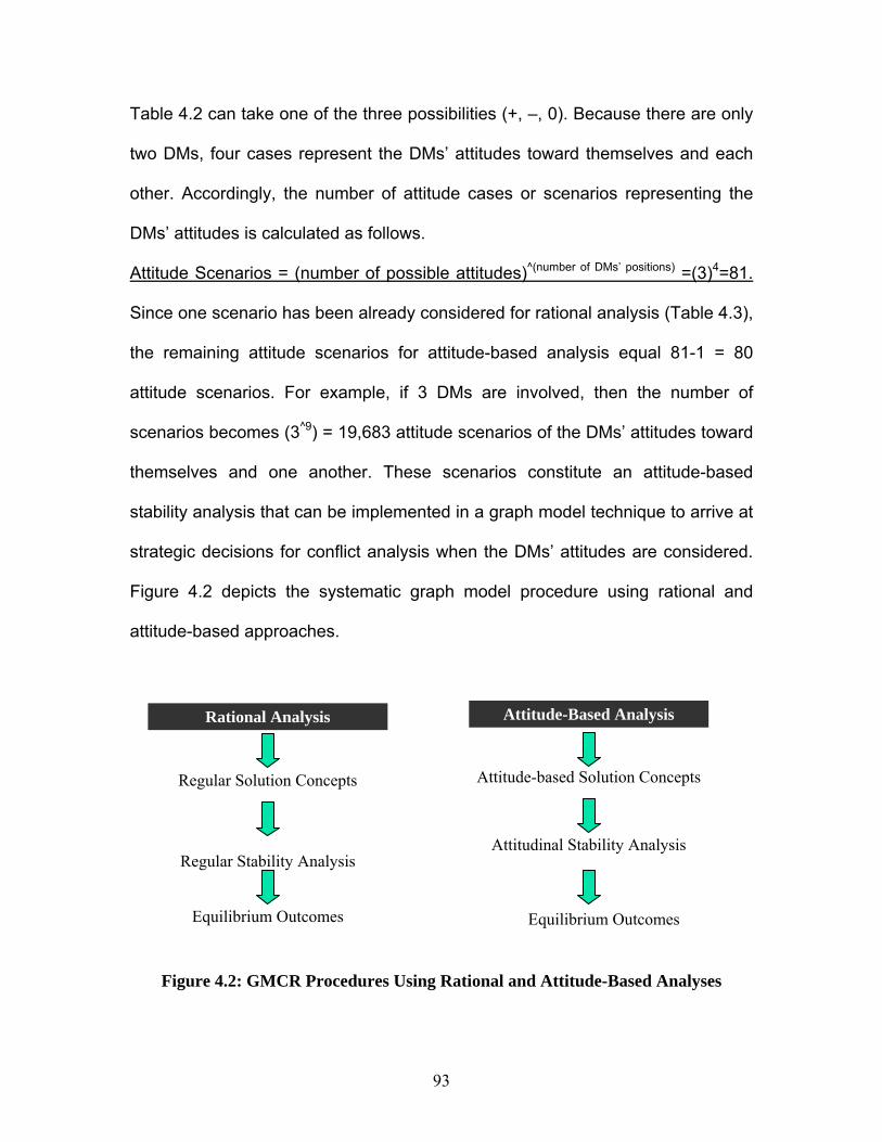
93
Table 4.2 can take one of the three possibilities (+, –, 0). Because there are only
two DMs, four cases represent the DMs’ attitudes toward themselves and each
other. Accordingly, the number of attitude cases or scenarios representing the
DMs’ attitudes is calculated as follows.
Attitude Scenarios = (number of possible attitudes)^(number of DMs’ positions) =(3)4=81.
Since one scenario has been already considered for rational analysis (Table 4.3),
the remaining attitude scenarios for attitude-based analysis equal 81-1 = 80
attitude scenarios. For example, if 3 DMs are involved, then the number of
scenarios becomes (3^9) = 19,683 attitude scenarios of the DMs’ attitudes toward
themselves and one another. These scenarios constitute an attitude-based
stability analysis that can be implemented in a graph model technique to arrive at
strategic decisions for conflict analysis when the DMs’ attitudes are considered.
Figure 4.2 depicts the systematic graph model procedure using rational and
attitude-based approaches.
Figure 4.2: GMCR Procedures Using Rational and Attitude-Based Analyses
Rational Analysis
Equilibrium Outcomes
Regular Solution Concepts
Regular Stability Analysis
Attitude-Based Analysis
Attitude-based Solution Concepts
Attitudinal Stability Analysis
Equilibrium Outcomes

94
4.4.5. Propositions on Relationships among Attitude-based Stability Types
One of the contributions of this research is to investigate how incorporating the
DMs’ attitudes into the stability concepts can change the relationship among the
stability concepts. In other words, when the attitudes of DMs change then the
different relationships are considered for the attitude-based stability concepts.
Three propositions on the relationships among attitude-based stability concepts
within the paradigm of the GMCR are proposed in the following. The proofs of
these propositions are presented by Inohara et al. (2008).
Proposition 1: Consider a graph model (N, C, (Si)i є N , (≥i) i є N) of a conflict and a
list e = (ei) i є N of attitudes ei of DM i for i є N. For i є N; Where N is the set of all
decision makers (DMs). C is the set of all states of the focal decision making
situation, where |C| ≥ 2. For i є N, Si is a function from C to the power set P(C) of
C such that c є Si(c) є P(C) for all c є C. Si is called the irreflexive reachable list
function of DM i є N and Si(c) is called the irreflexive reachable list of DM i є N
from c є C. ≥i is the preference of DM i є N on C. Accordingly,
)(eRNashiC ⊂
)(eRSMRiC ⊂
)(eRGMRiC and
)(eRNashiC ⊂
)(eRSEQiC ⊂
)(eRGMRiC . In other words, if
states 1 and 2, for example, are attitude-based Nash stable for DM i, they have
also attitude-based Symmetric Metarationality stability and further, they have
attitude-based General Metarationality stability. Moreover, if states 1 and 2, for
example, are attitude-based Nash stable for DM i, they have also attitude-based
Sequential stability and further, they have attitude-based General Metarationality
95
stability. It should be noted that these relationships among the relational stability
concepts are logically true from their definitions shown in Table 3.4
Proposition 2: Consider a graph model (N, C, (Si)i є N , (≥i) i є N) of a conflict and a
list e = (ei) i є N of attitudes ei of DM i for i є N. Assume that N = {1, 2} and the
DMs’ attitudes e = (ei) i є N are positive toward both themselves and other DMs.
Also, assume that DMs’ preferences ≥1 and ≥2 are transitive and antisymmetric.
Then, for i є N and c є C, c є)(eRNash
iC if and only if c є)(eRSEQ
iC .
Proposition 3: Consider a graph model (N, C, (Si)i є N , (≥i) i є N) of a conflict and a
list e = (ei) i є N of attitudes ei of DM i for i є N. Assume that N = {1, 2} and the
DMs’ attitudes e = (ei) i є N are negative toward both themselves and other DM.
Moreover, assume that DMs’ preferences ≥1 and ≥2 are transitive, antisymmetric,
and complete. Then, for i є N and c є C, c є)(eRNash
iC if and only if c є)(eRSEQ
iC .
The interpretation of Propositions 2 and 3 indicates that when DMs have totally
positive (or totally negative) attitudes toward themselves and one another, then
attitude-based Nash Stability (RNash) and attitude-based sequential stability
(RSEQ) are equivalent to each other, respectively.
4.5 Strategic Negotiation Methodology: A Brownfield Case Study
The attitude-based solution concepts, defined in the foregoing section, are
incorporated into GMCR technique to propose a negotiation methodology for

96
construction conflicts. To clarify the development of the methodology, the
procedure is demonstrated using a brownfield construction case study. More
information about brownfield negotiations have been provided in Subsection
2.2.3. In the proposed case study, the land of a privately owned property is
contaminated, and according to the municipality’s laws, the property is
considered a brownfield site which needs to be redeveloped in two steps:
remediation, which means that the contaminated soil must be replaced, and
redevelopment, which means that a new structure is to be constructed. Due to
the enormous costs, responsibilities, risks, and uncertainties involved with
brownfield construction, conflicts have often arisen between the current property
owner and Kitchener municipality. To illustrate these conflicts, a hypothetical
case study is considered in which the DMs are the owner and the government
(Yousefi et al., 2009). In the real world, the owner is very often a company, and
the government represents a body of people. However, since this research deals
with personal attitudes, it is more convenient to refer to the DMs as individuals.
Therefore, for the purpose of the analysis, the owner will be referred to as “she”,
“her”, “herself”, etc. The government will be referred to as “he”, “him”, “himself”,
etc.
With respect to the modeling stage of GMCR, first, the DMs involved in the
brownfield conflict and their available options are to be determined. It can be
assumed that both DMs in this case study have reviewed the different choices
available to them and selected the following options:
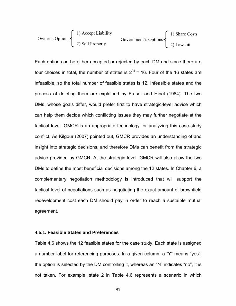
97
Each option can be either accepted or rejected by each DM and since there are
four choices in total, the number of states is 2^4 = 16. Four of the 16 states are
infeasible, so the total number of feasible states is 12. Infeasible states and the
process of deleting them are explained by Fraser and Hipel (1984). The two
DMs, whose goals differ, would prefer first to have strategic-level advice which
can help them decide which conflicting issues they may further negotiate at the
tactical level. GMCR is an appropriate technology for analyzing this case-study
conflict. As Kilgour (2007) pointed out, GMCR provides an understanding of and
insight into strategic decisions, and therefore DMs can benefit from the strategic
advice provided by GMCR. At the strategic level, GMCR will also allow the two
DMs to define the most beneficial decisions among the 12 states. In Chapter 6, a
complementary negotiation methodology is introduced that will support the
tactical level of negotiations such as negotiating the exact amount of brownfield
redevelopment cost each DM should pay in order to reach a sustaible mutual
agreement.
4.5.1. Feasible States and Preferences
Table 4.6 shows the 12 feasible states for the case study. Each state is assigned
a number label for referencing purposes. In a given column, a “Y” means “yes”,
the option is selected by the DM controlling it, whereas an “N” indicates “no”, it is
not taken. For example, state 2 in Table 4.6 represents a scenario in which
1) Accept Liability 2) Sell Property
Owner’s Options 1) Share Costs 2) Lawsuit
Government’s Options
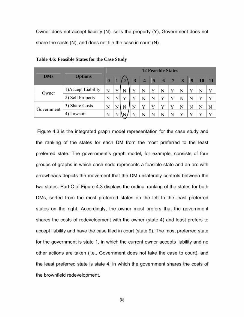
98
Owner does not accept liability (N), sells the property (Y), Government does not
share the costs (N), and does not file the case in court (N).
Table 4.6: Feasible States for the Case Study
12 Feasible States DMs Options
0 1 2 3 4 5 6 7 8 9 10 11
1)Accept Liability N Y N Y N Y N Y N Y N Y Owner 2) Sell Property N N Y Y N N Y Y N N Y Y 3) Share Costs N N N N Y Y Y Y N N N N Government 4) Lawsuit N N N N N N N N Y Y Y Y
Figure 4.3 is the integrated graph model representation for the case study and
the ranking of the states for each DM from the most preferred to the least
preferred state. The government’s graph model, for example, consists of four
groups of graphs in which each node represents a feasible state and an arc with
arrowheads depicts the movement that the DM unilaterally controls between the
two states. Part C of Figure 4.3 displays the ordinal ranking of the states for both
DMs, sorted from the most preferred states on the left to the least preferred
states on the right. Accordingly, the owner most prefers that the government
shares the costs of redevelopment with the owner (state 4) and least prefers to
accept liability and have the case filed in court (state 9). The most preferred state
for the government is state 1, in which the current owner accepts liability and no
other actions are taken (i.e., Government does not take the case to court), and
the least preferred state is state 4, in which the government shares the costs of
the brownfield redevelopment.
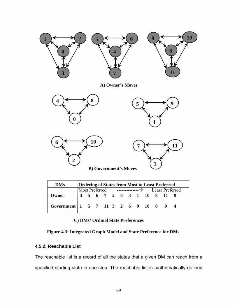
99
4.5.2. Reachable List
The reachable list is a record of all the states that a given DM can reach from a
specified starting state in one step. The reachable list is mathematically defined
0
1
3
2
8
9
11
10
4
5
7
6
0
4 8
1
5 9
2
6 10
3
7 11
A) Owner’s Moves
B) Government’s Moves
Figure 4.3: Integrated Graph Model and State Preference for DMs
DMs Ordering of States from Most to Least Preferred Most Preferred -------------- Least Preferred
Owner 4 5 6 7 2 0 3 1 10 8 11 9 Government 1 5 7 11 3 2 6 9 10 8 0 4
C) DMs’ Ordinal State Preferences
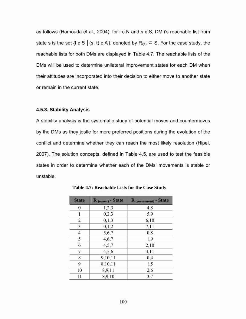
100
as follows (Hamouda et al., 2004): for i є N and s є S, DM i’s reachable list from
state s is the set {t є S │(s, t) є Ai}, denoted by Ri(s) ⊂ S. For the case study, the
reachable lists for both DMs are displayed in Table 4.7. The reachable lists of the
DMs will be used to determine unilateral improvement states for each DM when
their attitudes are incorporated into their decision to either move to another state
or remain in the current state.
4.5.3. Stability Analysis
A stability analysis is the systematic study of potential moves and countermoves
by the DMs as they jostle for more preferred positions during the evolution of the
conflict and determine whether they can reach the most likely resolution (Hipel,
2007). The solution concepts, defined in Table 4.5, are used to test the feasible
states in order to determine whether each of the DMs’ movements is stable or
unstable.
Table 4.7: Reachable Lists for the Case Study
State R (owner) - State R (government) - State 0 1,2,3 4,8 1 0,2,3 5,9 2 0,1,3 6,10 3 0,1,2 7,11 4 5,6,7 0,8 5 4,6,7 1,9 6 4,5,7 2,10 7 4,5,6 3,11 8 9,10,11 0,4 9 8,10,11 1,5 10 8,9,11 2,6 11 8,9,10 3,7

101
The mathematical forms for the solution concepts, shown in the centre column of
Table 4.5, are interpreted for the two DMs in this case as follows (Fraser and
Hipel, 1984):
1. Nash: In this situation, a DM has no Unilateral Improvement (UI) to make
from the state. In other words, the already selected strategy is the best
that can be chosen given the strategy selection of the other DM. A UI is
a state to which a particular DM can unilaterally move by a change in
strategy, assuming that the other DM’s strategy remains the same. The
Nash (rational) state is a stable outcome and is denoted by “Nash.”
2. Unstable: In this situation, the DM has at least one UI from which the
other DM can take no credible action that results in a less preferred state
for the given DM. An unstable outcome is denoted by “U.”
3. Sequentially sanctioned: In this case, for all UIs available to one DM,
credible actions can be taken by the other DM in which a less preferred
state than the one from which the DM is improving will be resulted. A
credible action is one that results in a more preferred state for the DM
taking the action. The possibility that a worse state could result from a
DM changing strategy deters the DM from unilaterally attempting a
position improvement and induces a stability type labeled as “SEQ.”
4.5.4. Analysis of the DMs’ Neutral Attitudes towards Each Other
The attitudes of the DMs can be integrated into the stability analysis using a
stability analysis tableau which consists of each DM’s state ranking (i.e.,
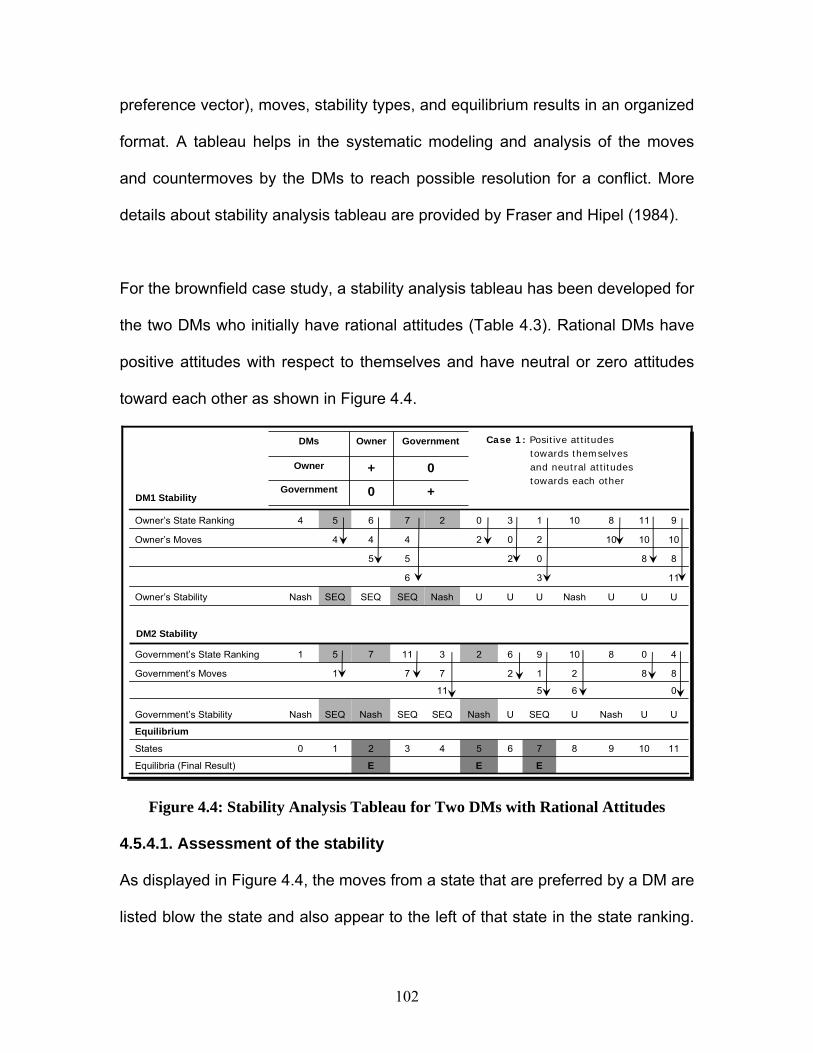
102
preference vector), moves, stability types, and equilibrium results in an organized
format. A tableau helps in the systematic modeling and analysis of the moves
and countermoves by the DMs to reach possible resolution for a conflict. More
details about stability analysis tableau are provided by Fraser and Hipel (1984).
For the brownfield case study, a stability analysis tableau has been developed for
the two DMs who initially have rational attitudes (Table 4.3). Rational DMs have
positive attitudes with respect to themselves and have neutral or zero attitudes
toward each other as shown in Figure 4.4.
11109876543210States
EEEEquilibria (Final Result)
Equilibrium
UUUNashUUUNashSEQSEQSEQNashOwner’s Stability
UUNashUSEQUNashSEQSEQNashSEQNashGovernment’s Stability
06511
88212771Government’s Moves
40810962311751Government’s State Ranking
1136
880255
101010202444Owner’s Moves
91181013027654Owner’s State Ranking
+
0
Government
0
+
Owner
Government
Owner
DMs Case 1: Positive attitudes towards themselves and neutral attitudes towards each other
DM1 Stability
DM2 Stability
Figure 4.4: Stability Analysis Tableau for Two DMs with Rational Attitudes
4.5.4.1. Assessment of the stability
As displayed in Figure 4.4, the moves from a state that are preferred by a DM are
listed blow the state and also appear to the left of that state in the state ranking.

103
The procedure for determining the types of stability are quite straightforward and
is extensively explained by Fraser and Hipel (1984). In order to check the Nash
stability, for example, Figure 4.4 is examined for states in the DMs’ state rankings
that do not have any moves listed under them. Since the DMs can not move from
these states, they are Nash stable and can be immediately marked with “Nash”.
In Figure 4.4, states 2, 4, and 10 are Nash stable for the owner, whereas states
1, 7, 2, and 8 are Nash stable for the government. Each of the remaining states
in the two state rankings can be assessed for their stability, which is normally
done for each DM sequentially. The owner can unilaterally move to state 4 from
state 5. However, the examination of the government’s vector reveals that the
government has an improvement from 4 to 8 and then to zero. As shown in the
owner’s state ranking (i.e., preference vector), both 8 and zero are less preferred
than 5, and the owner is therefore deterred from improving from 5 because of the
possibility that 8 or zero could result. Because the government would improve its
position by unilaterally moving from 4 to 8 or to zero, the sanction is credible.
Consequently, sate 5 is sequentially stable and a “SEQ” is written below state 5
in the owner’s state ranking. In the actual conflict, state 5 means that the owner
keeps sharing liability for the costs with the government who shares the costs of
brownfield redevelopment as well. Otherwise, if the owner does not share the
liability costs, then the government may either reject sharing the costs with the
owner or take the case to court. The same procedure applies for the government
regarding state 5. If the government unilaterally moves to state1, then the owner
has an improvement from 1 to 2 which is less preferred by the government and
104
more preferred by the owner. Thus, state 1 is sequentially sanctioned by the
owner and hence, outcome 5 is “SEQ” for the government. The same stability
analysis process is used to test the remaining states, as summarized in Table
4.8.
If a state possesses some types of stability for all DMs, it is called an equilibrium
state which constitutes a possible resolution to the conflict (Fraser and Hipel,
1984). All other outcomes are unstable for at least one of the DMs, and therefore
are not normally considered possible resolution. Equilibria are indicated by “E”
placed below the corresponding state (i.e., states 2, 5, and 7) on the last row in
the stability analysis tableau (Figure 4.4). An outcome that is unstable for at least
one DM is not marked by “E” In a stability tableau.
4.5.5. Analysis of the DMs’ Negative Attitudes towards Each Other
In the previous case, it was assumed that the DMs have rational attitudes toward
each other, and therefore, the DMs attitudes were not investigated. In this case
however, a situation is examined in which the DMs do not behave rationally and
the DMs’ various attitudes affect the outcome of their negotiation. To examine the
influence of DMs’ attitudes toward each other in this case, a situation is
considered in which the DMs change their attitudes from rational to relational
attitudes and possess negative attitudes toward each other and positive attitudes
toward themselves. In other words, the owner has a positive attitude toward
herself and negative attitude toward the government, whereas the government
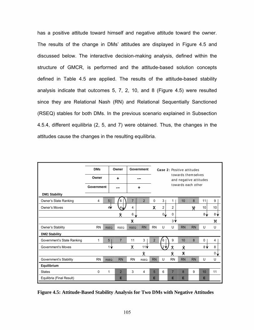
105
has a positive attitude toward himself and negative attitude toward the owner.
The results of the change in DMs’ attitudes are displayed in Figure 4.5 and
discussed below. The interactive decision-making analysis, defined within the
structure of GMCR, is performed and the attitude-based solution concepts
defined in Table 4.5 are applied. The results of the attitude-based stability
analysis indicate that outcomes 5, 7, 2, 10, and 8 (Figure 4.5) were resulted
since they are Relational Nash (RN) and Relational Sequentially Sanctioned
(RSEQ) stables for both DMs. In the previous scenario explained in Subsection
4.5.4, different equilibria (2, 5, and 7) were obtained. Thus, the changes in the
attitudes cause the changes in the resulting equilibria.
11109876543210States
EEEEEEquilibria (Final Result)
UURNRNRNURNRSEQRNRNRSEQRNGovernment’s Stability
Equilibrium
UURNRNUURNRNRSEQRSEQRSEQRNOwner’s Stability
0657
882121171Government’s Moves
40810962311751Government’s State Ranking
1135
880065
101010222444Owner’s Moves
91181013027654Owner’s State Ranking
+
-–
Government
-–
+
Owner
Government
Owner
DMs
X
X
X
X
XX
XXX
XX
Case 2: Positive attitudes towards themselves and negative attitudes towards each other
DM1 Stability
DM2 Stability
Figure 4.5: Attitude-Based Stability Analysis for Two DMs with Negative Attitudes

106
4.5.5.1. Assessment of the stability
As shown in Figure 4.5, below a given state in the state ranking for each DM are
the DM’s possible moves or the Total Relational Reply (TRR) lists determined
according to the attitudes shown above the tableau in Figure 4.5. The stability of
each sate in the sate ranking has been evaluated and shown below the DMs’
state ranking. State 6, circled in Figure 4.5, is assessed, for example, for the
owner. According to the reachable list of the owner in Table 4.7, Rowner (6) = {4, 5,
7}. As the owner has a positive attitude with respect to herself, the owner has a
devoting preference (defined in Subsection 4.4.2) toward herself. From the
ranking of the states in Figure 4.5, it can be seen that states 4 and 5 are more
preferred and 7 is less preferred to state 6 for the owner within the reachable list
for state 6, therefore, 4, 5 RP (eowner, owner= +) 6. Since the owner has a negative
attitude toward the government, the owner wants to ensure that her improving
move from 6 to 4 or 5 will not benefit her opponent. From the ordering of the
states for the government in Figure 4.5, it can be seen that 5 is more preferred
and 4 is less preferred to 6 and thus, 4 RP (eowner, government= -) 6. It can be
concluded that 4 TRP (eowner) 6 and thus TRR (6)owner ={4}, which is circled in
Figure 4.5. The same procedure is carried out for other states to determine TRR
for each DM. Once TRR (6) for the owner is obtained, the stability of state 6 is
examined. If the owner moves from 6 to 4, then the government can move from 4
to 8. Although 8 is less preferred to 6 for the government, state 8 is also less
preferred to 6 for the owner and because the owner has a positive attitude
toward herself she is deterred to move from 6 to 4. Thus, state 6 becomes RSEQ
107
for the owner and an “RSEQ” is written below state 6 for the owner’s state
ranking.
The stability of state 6 is now assessed for the government. According to his
reachable list in Table 4.7, Rgovernment (6) = {2, 10}. As the government has a
positive attitude with respect to himself (Figure 4.5), he has a devoting
preference toward himself. It can be seen from his state ranking that state 2 is
more preferred and 10 is less preferred to state 6 within the reachable list for
state 6. As such, 2 RP (egov.,gov.= +) 6. Since the government has a negative
attitude toward the owner, he wants to ensure that his improving move from 6 to
2 will not benefit his opponent (the owner). It can be noticed from the ordering of
the states for the owner that 2 is less preferred to 6, and thus, the government
can escalate the conflict by unilaterally moving to state 2. It should be noted that
the government is not deterred to move to 2 from 6 because state 2 is “RN” for
the owner. State 6 then becomes unstable for the government and an “U” is
written below state 6 for the government’s state ranking. It can be concluded that
2 TRP (egov.) 6, so TRR (6)gov. ={2}. The same stability analysis is performed for
the other states, and the results are summarized in Table 4.8.
4.5.6. Analysis of the DMs’ Positive Attitudes towards Each Other
A situation is now considered in which both DMs have positive attitudes with
respect to themselves and toward each other. Such situation is in contrast to the
preceding situation in which the DMs had negative attitudes toward each other.

108
The objective is to examine how the possible strategic negotiation outcome
changes when the DMs’ attitudes change. The interactive decision-making
analysis, defined within the structure of GMCR, is performed and the attitude-
based solution concepts defined in Table 4.4 are applied. Accordingly, states 1,
2, 4, and 5, shown in Figure 4.6, were resulted as equilibria since they are
Relational Nash (RN) stable for the DMs. It should be remembered that in the
previous scenarios, different equilibria were obtained. It can again be seen that
the changes in the DMs’ attitudes cause corresponding changes in the resulting
equilibria. In this scenario, states 1, 2, 4, and 5 constitute equilibrium states,
indicating that the positive attitudes of the DMs have provided both DMs with
better equilibrium states; thus, the DMs may reach a better strategic resolution to
their conflict.
11109876543210States
EEEEEquilibria (Final Result)
RNRNRNUURNRNUURNRNRNGovernment’s Stability
Equilibrium
URNURNRNRNURNUURNRNOwner’s Stability
06511
88212771Government’s Moves
40810962311751Government’s State Ranking
1036
880044
111010222554Owner’s Moves
91181013027654Owner’s State Ranking
+
+
Government
+
+
Owner
Government
Owner
DMs
X
X
X
XX
XXX
XX
Case 3: Positive attitudes towards themselves and positive attitudes towards each other
DM1 Stability
DM2 Stability
XX
XXX
XX X
X
Figure 4.6: Attitude-Based Stability Analysis for Two DMs with Positive Attitudes
109
4.5.6.1. Assessment of the stability
For this situation, the stability of state 6, circled in Figure 4.6, is evaluated for
both DMs. It should be noted that state 6 was already examined for previous
situation in Subsection 4.5.5. According to the reachable list of the owner in
Table 4.7, Rowner (6) = {4, 5, 7}. Because the owner has a positive attitude with
respect to herself, she has a devoting preference (defined in Subsection 4.4.2)
toward herself. From the ranking of the states in Figure 4.6, it can be seen that
states 4 and 5 are more preferred and 7 is less preferred to state 6 for the owner
within the reachable list for state 6, so 4, 5 RP (eowner, owner= +) 6. Since the owner
has also a positive attitude toward the government, the owner wants to ensure
that her move from 6 to 4 or 5 will not lower her opponent’s position. Thus, from
the ordering of the states for the government in Figure 4.6, it can be seen that 5
is more preferred and 4 is less preferred to 6 and thus, 5 RP (eowner, government= +)
6. It means that the owner’s move from 6 to 5 benefits the DMs and, thus, the
owner has a possible move from 6 to 5. It is concluded that, 5 TRP (eowner) 6, so
TRR (6)owner ={5}, circled in Figure 4.6.
The stability of state 6 is now assessed for the government. According to his
reachable list in Table 4.6, Rgovernment (6) = {2, 10}. Because the government has
a positive attitude with respect to himself (Figure 4.6), he has a devoting
preference toward himself. It can be seen from his ranking states that state 2 is
more preferred and 10 is less preferred to state 6 within the reachable list for
state 6, so 2 RP (egov.,gov.= +) 6. Since the government has a positive attitude
110
toward the owner, he wants to ensure that his unilateral move from 6 to 2 will not
lower his opponent’s position. Thus, it can be seen from the ordering of the
states for the owner that 2 is less preferred to 6, and thus the government is
deterred from escalating the conflict by moving to state 2. Accordingly, the
government has no possible move from state 6 according to his attitude.
Once the TRR lists for the DMs are determined, the stability of state 6 is
examined. If the owner moves from 6 to 5, the government has no move from 5
and, therefore, the owner can move from 6 to 5 and, thus, state 6 becomes
unstable for the owner. Because the government has no move from 6, state 6
becomes RNASH stable for the government as shown in Figure 4.6. It can be
concluded that Φ TRP (egov.) 6, so TRR (6)gov. ={ Φ }. The same stability analysis
has been performed for the other states, and the results are summarized in Table
4.8. Separate stability analyses for the owner and the government are also
shown in Tables 4.9 and 4.10, respectively. The resulting outcomes of the three
situations in the case study are discussed as follows.
4.6. Discussion of the Resulting Strategic Decisions
In the previous section, a brownfield case study was studied considering three
attitude cases: 1) the DMs had neutral (zero) attitudes toward each other; 2) they
had negative attitudes toward each other; and 3) they had positive attitudes
toward each other. The objective is to examine how changes in the DMs’
attitudes can influence the negotiation outcome.

111
Table 4.8: Summary of the Stability Analysis for the Case Study Note 1: “O” stands for owner and “G” stands for government. Note 2: The grayed states are equilibria for each situation. Note 3: States with gray cells stand for equilibria or possible solutions
DMs’ Attitudes toward each other State
DMs Neutral (zero) Negative Positive
O
Unstable: O is not deterred to move to 2, because 2 is Nash stable state for G.
Stable: O is deterred to move to her only UI state 2, because 2 is more preferred to 0 for G and O does not want to improve G’s position.
Unstable: to improve her position and G’ position, O moves to her only state 2 which is more preferred state to 0 for O and G.
0
G
Unstable: if G moves to 8, O can countermove from 8 to 10 which is more preferred state than 8 for G.
Unstable: to lower O’s position , G moves to his only state 8 which is less preferred to 0 for O.
Stable: G is deterred to move to her only UI state 8, because 8 is less preferred to 0 for O and G does not want to lower O’s position.
O Unstable: O is not deterred to move to 2, because 2 is Nash stable state for G.
Unstable: to lower G’s position, O moves to 2,0, and 3 which are less preferred to 1 for G.
Stable: O is deterred to move to UIs 2, 0, or 3 because they are less preferred to 1 for G, and O does not want to lower G’s position.
1
G Nash Stable: no unilateral moves Nash Stable: no improvement moves within G’ reachable list
Nash Stable: no improvement moves within G’ reachable list
O Nash Stable: no unilateral moves Nash Stable: no improvement moves within O’ reachable list
Nash Stable: no improvement moves within O’ reachable list 2
G Nash Stable: no unilateral moves Nash Stable: no improvement moves within G’ reachable list
Nash Stable: no improvement moves within G’ reachable list
O Unstable: O is not deterred to move to 2, because 2 is Nash stable state for G.
Unstable: to lower G’s position, O moves to 0 and 2 which are less preferred states to 3 for G.
Stable: O is deterred to move to UIs 2 or 0, because they are less preferred to 3 for G, and O does not want to lower G’s position.
3
G
Stable: if G moves to UIs 7 or 11, then O countermoves to states 4 and 10 respectively which are less preferred to 3 for G.
Stable: G is deterred to move to 11 since O has a credible sanction from 11 to 10 which is less preferred to 3 for G.
Unstable: to improve his position and O’ position, G moves to UI state 7 which is more preferred state to 3 for G and O; also, G is deterred to lower O’s position by moving to his UI state 11.
O Nash Stable: no unilateral moves Nash Stable: no improvement moves within O’ reachable list
Nash Stable: no improvement moves within O’ reachable list
4 G
Unstable: if G moves to 8, O can countermove from 8 to 10 which is more preferred state than 4 for G.
Unstable: to lower O’s position , G moves to 8 and 0 which are less preferred to 4 for O.
Stable: G is deterred to move to UIs 8 or 0, because they are less preferred to 4 for O, and G does not want to lower O’s position.
O
Stable: if O moves to UI 4, then G countermoves from 4 to 8 or 0 which are less preferred to 5 for O.
Stable: O is deterred to move to 4 since G has a credible sanction from 4 to 8 which is less preferred to 5 for O.
Stable: O is deterred to move to her only UI state 4, because 4 is less preferred to 5 for G, and O does not want to lower G’s position.
5
G Stable: if G moves to UI 1, then O countermoves from 1 to 2, 0, or 3 which are less preferred to 5 for G.
Stable: G is deterred to move to 1 since O has a credible sanction from 1 to 2 which is less preferred to 5 for G.
Nash Stable: no improvement moves within G’ reachable list
O Stable: if O moves to UI 4 or 5, then G can countermove from 4 or 5 to 8, 0, or 1 which are less preferred to 6 for O.
Stable: O is deterred to move to 4 since G has a credible sanction from 4 to 8 which is less preferred to 6 for O.
Unstable: O moves to 5 to improve her own and her opponent’ positions. 6
G
Unstable: G is not deterred to move to 2, because 2 is Nash stable state for O.
Unstable: to lower O’s position, G moves to his only state 2 which is less preferred state to 6 for O.
Stable: G is deterred to move to his only UI state 2, because 2 is less preferred to 6 for O, and G is deterred to lower O’s position.
7 O
Stable: if O moves to UIs 4, 5, or 6 then G can countermove from 4, 5, and 6 to 8, 0, 1, and 2 respectively which are less preferred states to 7 for O.
Stable: O is deterred to move to 4 or 6 since G has credible sanction from 4 and 6 to 8 and 2 respectively. 8 and 2 are less preferred to 7 for O.
Unstable: to improve her position and G’ position, O moves to UI state 5 which is more preferred state to 7 for G and O; also, O is deterred to lower G’s position by moving to her UIs 4 or 6 which are less preferred to 7 for G.
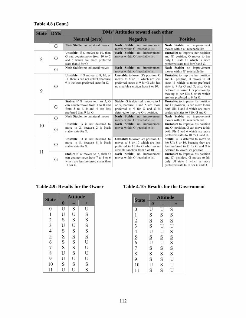
112
DMs’ Attitudes toward each other State
DMs Neutral (zero) Negative Positive
G Nash Stable: no unilateral moves Nash Stable: no improvement moves within G’ reachable list
Nash Stable: no improvement moves within G’ reachable list
O Unstable: if O moves to 10, then G can countermove from 10 to 2 and 6 which are more preferred state than 8 for O.
Nash Stable: no improvement moves within O’ reachable list
Unstable: to improve her position and G’ position, O moves to her only UI state 10 which is more preferred state to 8 for O and G.
8
G Nash Stable: no unilateral moves Nash Stable: no improvement moves within G’ reachable list
Nash Stable: no improvement moves within G’ reachable list
O
Unstable: if O moves to 8, 10, or 11, then G can not deter O because 9 is the least preferred state for O.
Unstable: to lower G’s position, O moves to 8 or 10 which are less preferred states to 9 for G who has no credible sanction from 8 or 10.
Unstable: to improve her position and G’ position, O moves to UI state 11 which is more preferred state to 9 for G and O; also, O is deterred to lower G’s position by moving to her UIs 8 or 10 which are less preferred to 9 for G.
9
G Stable: if G moves to 1 or 5, O can countermove from 1 to 0 and from 5 to 4. 0 and 4 are less preferred than 9 for G.
Stable: G is deterred to move to 1 or 5, because 1 and 5 are more preferred to 9 for O and G is deterred to improve O’s position.
Unstable: to improve his position and O’ position, G can move to his both UIs 1 and 5 which are more preferred states to 9 for G and O.
O Nash Stable: no unilateral moves Nash Stable: no improvement moves within O’ reachable list
Nash Stable: no improvement moves within O’ reachable list
10 G
Unstable: G is not deterred to move to 2, because 2 is Nash stable state for O.
Nash Stable: no improvement moves within G’ reachable list
Unstable: to improve his position and O’ position, G can move to his both UIs 2 and 6 which are more preferred states to 10 for G and O.
O Unstable: O is not deterred to move to 8, because 8 is Nash stable state for G.
Unstable: to lower G’s position, O moves to 8 or 10 which are less preferred to 11 for G who has no credible sanction from 8 or 10.
Stable: O is deterred to move to her UIs 8 or 10, because they are less preferred to 11 for G, and O is deterred to lower G’s position. 11
G Stable: if G moves to 7, then O can countermove from 7 to 4 or 6 which are less preferred states than 11 for G.
Nash Stable: no improvement moves within G’ reachable list
Unstable: to improve his position and O’ position, G moves to his only UI state 7 which is more preferred state to 11 for G and O.
Table 4.9: Results for the Owner Table 4.10: Results for the Government
Attitude State0 – +
0 1 2 3 4 5 6 7 8 9 10 11
U S S S U S U S S S U S
U S S U U S U S S S S S
S S S U S S S S S U U U
Attitude State 0 – +
0 1 2 3 4 5 6 7 8 9 10 11
U U S U S S S S U U S U
S U S U S S S S S U S U
U S S S S S U U U U S S
Table 4.8 (Cont.)

113
To achieve this objective, the attitude-based stability analysis was performed.
Due to the changes in the DMs’ attitudes regarding the three attitude cases,
three different sets of outcomes, were obtained. The resulting equilibrium states
are reviewed and one agreed-upon equilibrium state as the most beneficial
strategic decision of the brownfield negotiation is determined. The results of the
stability analysis for each attitude case are shown in Figure 4.7, and a brief
discussion is provided in the following subsections.
+
0
g
0
+
o
g
o
DMs
+
–
g
–
+
o
g
o
DMs
+
+
g
+
+
o
g
o
DMs
Stability AnalysisStability Analysis
Stability AnalysisStability Analysis
Stability AnalysisStability Analysis
Attitude Matrix
Neutral
Negative
Positive
GMCREquilibrium Sates
(Potential Solutions)
2, 5, 7
2, 5, 7, 8, 10
1, 2, 4, 5
Note: Decision 2 is considered a beneficial strategic decision
Figure 4.7: Three Sets of Equilibria for Three Attitude Cases
4.6.1. Attitude Case 1
In this attitude case, the DMs have neutral (zero) attitudes toward each other.
Using the proposed attitude-based stability analysis, three possible strategic
solutions (i.e., states 2, 5, and 7) were obtained for this case as shown in Figure
4.7. The DMs evaluate the three resulting decision options and try to find the

114
most beneficial strategic outcome for the conflict. One key outcome of the
stability analysis for this case study is outcome 2, which means that the owner
does not accept liability and sells the property, and that the government does not
share the costs of the brownfield redevelopment and does not take the case to
court. Another possible solution to the conflict is outcome 5, which corresponds
to saying that the owner accepts her liability regarding the property remediation
and does not sell her property, and the government shares the costs of
remediation and does not file a court case. The third possible solution to the
conflict is outcome 7, which means that the owner accepts liability and the
government shares the costs. Once the land is remediated, the owner sells the
property to the government and the government does not take the case to court.
4.6.2. Attitude Case 2
In this attitude case, the DMs have negative attitudes toward each other. The
results of the proposed attitude-based stability analysis show that the set of
equilibria changed toward more hostile possible solutions when the DMs
changed their attitudes from neutral to negative toward each other. In this case,
the equilibrium set includes 5, 7, 2, 8, and 10. It is observed that outcomes 2 and
5 (possible solutions in Case 1) are also resulted and thereby, are still
considered in this case as possible solution options although the DMs have
changed their attitudes. It can also be noticed that outcomes 8 and 10 are less
preferred solutions for both DMs in comparison to outcomes 2, 5, and 7.
Equilibrium state 8 for the conflict corresponds to saying that the owner neither

115
accepts liability nor sells her property and that the government does not share
any cost and takes the case to court. In other words, both DMs escalate the
conflict because they have negative attitudes toward each other. Since they have
positive attitudes only with respect to themselves, they strive to improve their
own position and lower their opponents’ position in the conflict. Equilibrium state
10 also corresponds to saying that the owner does not accept liability and sells
the property and that the government rejects any cost sharing and tries to lower
the owner’s position by taking the case to court. Hence, the owner rejects liability
since she considers liability acceptance as a positive point for the government,
and this positive move is in contrast with her negative attitude toward the
government. As can be seen, if DMs with negative attitudes interact, the strategic
solutions that result are more hostile.
4.6.3. Attitude Case 3
With respect to this attitude case, the DMs have positive attitudes toward
themselves and each other. In this scenario, outcomes 1, 2, 4, and 5 are
considered as possible solution options for the conflict. Equilibrium state 1 means
that the owner accepts liability and does not sell her property and that the
government does not share the costs and does not take the case to court.
Equilibrium state 4 means that the owner neither accepts liability nor sells her
property, and that the government does accept all the costs and does not take
the case to court. It can be observed that better possible solution options were
obtained in this attitude case due to the positive attitudes of the DMs toward each
116
other. It is noted that outcomes 2 and 5 (possible solutions in Cases 1 and 2) are
also resulted in this case and thereby, are still considered as possible solution
options although the DMs have changed their attitudes. Considering the results
of the three attitude cases, the following observations are considered:
1. The increase in the number of solution options (equilibria) in a conflict
may help the involved DMs choose a better possible solution from the
resulting equilibrium states;
2. Outcomes 2, 4, and 5 are more preferred for both DMs than the outcomes
8 and 10 obtained from Case 2. In other words, the positive attitudes of
the DMs toward themselves and each other not only mitigate the degree
of hostility involved in outcomes 8 and 10 but also shift the range of
solution options in the DMs’ state ranking (i.e., preference vector) from
right (less preferred states) to the left (more preferred states). Considering
the DMs’ state rankings in Figure 4.3 c, it can be seen that the positive
attitudes of the DMs help shift the set of equilibria in the state rankings
from the subset of 5, 7, 2, 8, and 10 on the right to the better subset of 1,
2, 4, and 5 on the left for both DMs;
3. One important observation is that the resulting equilibria for the three
scenarios share equilibria 2 and 5, as shown in Figure 4.7. Solution
options 2 and 5 are the only common equilibria obtained from the stability
analysis based on three different DM attitudes because no matter what
type of attitudes (neutral, negative, or positive) the DMs have toward each
other, these outcomes provide equilibrium solutions. Thus, the DMs

117
involved may (or may not) consider each of the equilibrium states a
reasonable decision and a strategic outcome of their conflict and may
cooperatively continue their interactive negotiation to develop a tactical
level of tradeoffs for the conflicting issue involved in solutions 2 and 5. It
should be noted that the only conflicting issue in equilibrium state 2 is that
the owner sells the property as indicated by “Y” in Table 4.6. The issues
indicated by “N” for that equilibrium are not considered to be conflicting
issues. Equilibrium state 5 consists of two conflicting issues indicated by
two “Y” in this outcome: the amount of liability that the owner accepts and
the amount of cost that the government shares. From the two possible
solutions 2 and 5, the owner and the government can strategically agree
on outcome 2, which has only one conflicting issue, and continue to
negotiate in order to find a concession price for the owner’s property.
Such negotiations have to be carried out at the tactical level rather than at
the strategic decision-making level. The tactical level of negotiation
methodology involving two DMs is proposed in Chapter 6.
4.7. Summary
The primary objective of this chapter was to present meaningfully and
constructively the strategic level of the proposed negotiation methodology
involving two decision makers. The proposed methodology systematically
employs GMCR and incorporates the decision makers’ attitudes into the
methodology. In this chapter, the proposed negotiation framework was initially

118
introduced. As shown in Figure 4.1, three major components constitute the
proposed negotiation framework: understanding the construction negotiation,
developing an attitude-based construction negotiation methodology, and
designing a negotiation decision support system. The requirements for
understanding construction negotiations were explained, and the characteristics
of construction negotiations as well as construction participants were highlighted.
An attitude-based negotiation methodology at the strategic level was then
developed. To demonstrate the advantages of the proposed methodology, a
case study of a brownfield construction conflict involving two decision makers
was used in order to develop the negotiation methodology. The brownfield case
study has been also used in Chapter 6 to develop a negotiation methodology at
the tactical level when.
The proposed negotiation methodology at the strategic level has been developed
when only two decision makers are involved in the negotiation process to arrive
at a mutual strategic agreement. The proposed strategic negotiation
methodology in this chapter has been adapted and further developed, as
discussed in Chapter 5 in order to include multiple decision makers involved in
strategic negotiations.
119
CHAPTER 5 Attitude-Based Strategic Negotiation Involving Multiple Decision Makers
5.1. Introduction
In this chapter, the negotiation methodology, presented in Chapter 4 for two
Decision Makers (DMs), is developed further, and an attitude-based negotiation
methodology for multiple DMs and multiple conflicting issues is proposed. A real
life brownfield negotiation involving multiple DMs is used to clearly demonstrate
the advantages of the proposed methodology. The historical background of the
case study is therefore summarized, and the DMs involved, along with their
options and the conflicting issues are also presented. The proposed negotiation
methodology has been developed using an attitude-based Graph Model for
Conflict Resolution which has been expanded to include both qualitative and
quantitative analyses.
5.2. Real-Life Brownfield Case Study
Downtown Kitchener, located in southern Ontario has a number of aging
buildings, older industrial plants, brownfield lands, and underutilized sites that
were once productive contributors to the economy of the community. These
lands and buildings need to be brought back into production.

120
The case study used for this research is a brownfield land at the corner of King
Street and Victoria Street in Kitchener. For approximately 75 years, B.F.
Goodrich manufactured plastic and rubber components for the automotive
industry in a five-story, 5,000 m2 factory and several adjacent outbuildings on an
8-hectare site near the intersection of King and Victoria Street, as shown in
Figure 5.1. Large quantities of fuels and chemicals were used and stored at the
site, including solvents. Because of the lack of proper maintenance and the
absence of environmental regulations in 1919 when B.F. Goodrich began
operation, the land became contaminated, in large part from 75 years of leaks
and spills from underground storage tanks, most of which contained naphtha,
and some of which held chlorinated solvents and heavy metals. During the
remediation process, elevated concentrations of beryllium and zinc, and to a
lesser extent, copper were detected in the upper 1.0 m of soil, primarily on the
south side of the site.
Figure 5.1: Satellite Image of the Former Brownfield Site
N
Constructed UW School of Pharmacy
Former Brownfield Site Heavily Contaminated
121
In 1983, B.F. Goodrich sold the site (factory) to Epton. As part of the transaction,
Goodrich Canada indemnified Epton for specific claims that could arise from
environmental contamination that may have occurred prior to 1983. In 1993,
Goodrich (USA) spun off its Geon Vinyl Division as an independent publicly
traded U.S. corporation: the Geon Company. Geon Canada thus became the
successor to the interests of Goodrich Canada with respect to the brownfield site.
The Geon Company later became PolyOne Corporation, and Geon Canada was
renamed PolyOne Company.
In March of 1994, Epton demanded that PolyOne accept responsibility for the
environmental contamination at the site, based on the indemnifications from
Goodrich to Epton in the 1983 sale of the facility. Epton was experiencing
financial difficulties at the time and was operating pursuant to a proposal made in
1993 under the Bankruptcy and Insolvency Act. Although PolyOne had no
obligation to respond affirmatively to Epton’s demand, Epton and PolyOne
decided to undertake a joint environmental investigation in order to clean up the
land since both parties already knew that the site was contaminated. They
agreed that costs were to be split 50-50 and then reallocated later when and if
liability was established. It should be mentioned that no legal remediation
requirements had been enacted by any governmental organization at that time,
but future Ministry of Environment (MOE) involvement was probated, in which
case, parties involved, such as PolyOne and Epton, could be asked to complete
the brownfield remediation process.

122
5.2.1. The Causes of the Conflict
Despite its initial agreements with PolyOne and its primary responsibility for the
cleanup, Epton filed for bankruptcy in 1995 and disputes therefore arose as to
the allocation of the environmental liabilities of the parties involved, including
PolyOne, the creditors, the banks, the Trustee in bankruptcy, and the interim
operator. In other words, when Epton, the party primarily responsible, filed for
bankruptcy, the potential liability for the environmental conditions at the site fell
upon numerous other parties, including prior property owners (including
Goodrich/Geon), the Trustee itself, secured creditors, specific interim operators,
and others that had been involved with plant operations over the years. In
addition, the property itself became an albatross. Anyone taking possession,
control, or ownership of any of the Epton site automatically became potentially
responsible for the existing contamination at the site. Therefore, all the parties
involved denied responsibility for brownfield liabilities. Moreover, Epton’s
creditors and mortgagees, and the The City of Kitchener possessed liens for
several million dollars against the real property and other assets. The existence
of the liens, claims, and counterclaims, as well as the issue of allocating
environmental liability, virtually guaranteed disputes among the parties involved.
For example, the The City of Kitchener (The City) had liens of over $1 million on
the property, including the debt of accruing property taxes and unpaid hydro
charges. In November 1995, the Trustee in bankruptcy wrote to The City officials,
informing them that the Epton buildings would be stripped, the utilities and fire
protection would be terminated, and the site would be abandoned.

123
5.3. Identifying DMs and Their Options
The brownfield negotiations between the The City and PolyOne concerning the
status of the property were started during 1995. It is therefore important to note
that this real-life negotiation is modeled and analyzed based on the information
available at that time. The The City had become increasingly concerned about
the abandoned buildings and the contaminated land, which presented an
extreme fire and safety hazard. On the other hand, PolyOne showed its
willingness to take responsibility for remediating the land on its own under
specific conditions: 1) full control of the land during the remediation so that it
would be fast and inexpensive, they would then transfer the site to the The City
by donating it for public use; 2) other incentives from the The City to facilitate the
remediation process.
Although PolyOne had the option of litigation, they concluded that even if they
assumed the entire burden of the site remediation, it would probably cost less
than even a small share of the enormous transactional costs of a traditional
lengthy litigation-driven remedy.
Because the The City feared that PolyOne would be discouraged from taking
possession if they had to pay the back taxes, the The City offered a write-off of
the taxes. In order to facilitate the remediation process, the land was also
transferred from the Trustee to PolyOne for only one dollar.
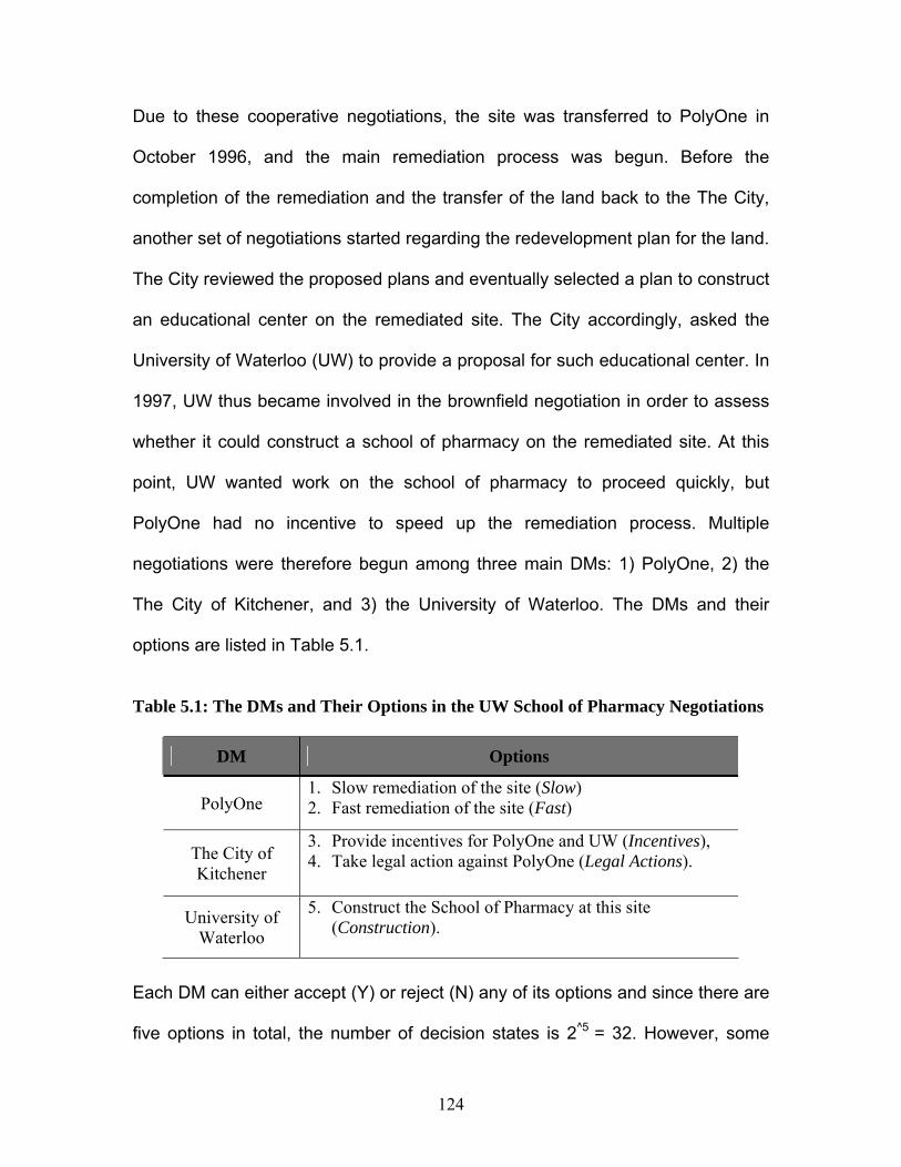
124
Due to these cooperative negotiations, the site was transferred to PolyOne in
October 1996, and the main remediation process was begun. Before the
completion of the remediation and the transfer of the land back to the The City,
another set of negotiations started regarding the redevelopment plan for the land.
The City reviewed the proposed plans and eventually selected a plan to construct
an educational center on the remediated site. The City accordingly, asked the
University of Waterloo (UW) to provide a proposal for such educational center. In
1997, UW thus became involved in the brownfield negotiation in order to assess
whether it could construct a school of pharmacy on the remediated site. At this
point, UW wanted work on the school of pharmacy to proceed quickly, but
PolyOne had no incentive to speed up the remediation process. Multiple
negotiations were therefore begun among three main DMs: 1) PolyOne, 2) the
The City of Kitchener, and 3) the University of Waterloo. The DMs and their
options are listed in Table 5.1.
Table 5.1: The DMs and Their Options in the UW School of Pharmacy Negotiations
DM Options
PolyOne 1. Slow remediation of the site (Slow) 2. Fast remediation of the site (Fast)
The City of Kitchener
3. Provide incentives for PolyOne and UW (Incentives), 4. Take legal action against PolyOne (Legal Actions).
University of Waterloo
5. Construct the School of Pharmacy at this site (Construction).
Each DM can either accept (Y) or reject (N) any of its options and since there are
five options in total, the number of decision states is 2^5 = 32. However, some
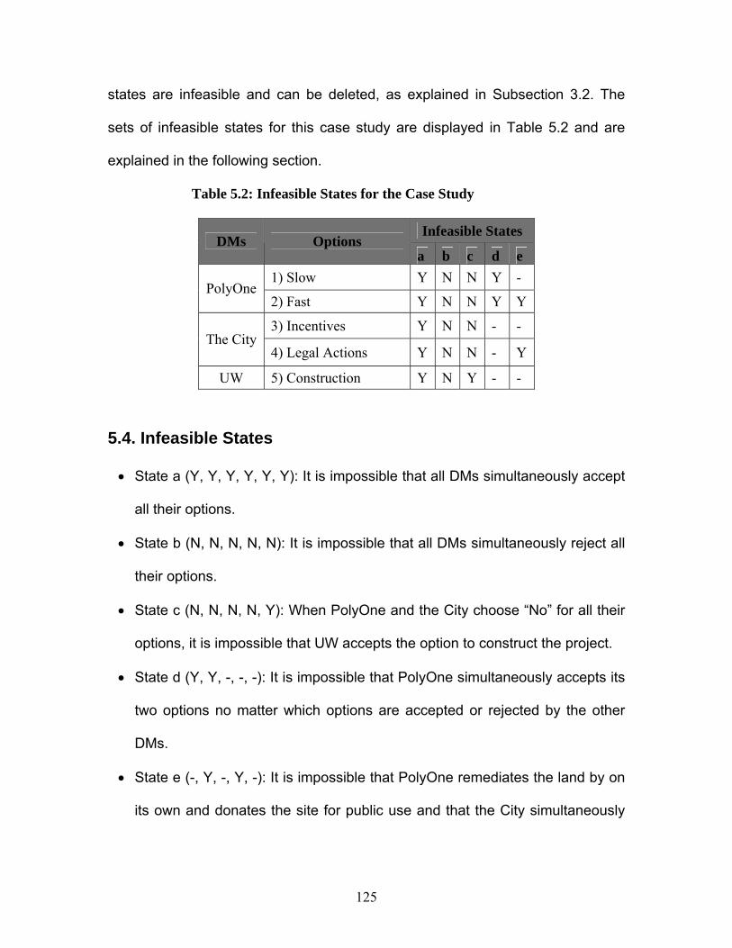
125
states are infeasible and can be deleted, as explained in Subsection 3.2. The
sets of infeasible states for this case study are displayed in Table 5.2 and are
explained in the following section.
Table 5.2: Infeasible States for the Case Study
Infeasible States DMs Options
a b c d e 1) Slow Y N N Y -
PolyOne 2) Fast Y N N Y Y
3) Incentives Y N N - - The City
4) Legal Actions Y N N - Y
UW 5) Construction Y N Y - -
5.4. Infeasible States
• State a (Y, Y, Y, Y, Y, Y): It is impossible that all DMs simultaneously accept
all their options.
• State b (N, N, N, N, N): It is impossible that all DMs simultaneously reject all
their options.
• State c (N, N, N, N, Y): When PolyOne and the City choose “No” for all their
options, it is impossible that UW accepts the option to construct the project.
• State d (Y, Y, -, -, -): It is impossible that PolyOne simultaneously accepts its
two options no matter which options are accepted or rejected by the other
DMs.
• State e (-, Y, -, Y, -): It is impossible that PolyOne remediates the land by on
its own and donates the site for public use and that the City simultaneously

126
takes legal action no matter which options are accepted or rejected by the
other DMs.
According to the above reasoning, the number of infeasible states is 14 and they
have been removed from the total number of states (2^5 = 32). The remaining 18
feasible states are labeled and listed from 0 to 17 and are shown in Table 5.3 in
which each column represents a state for which Y means “Yes” and N indicates
“No.”
Table 5.3: Resulting Feasible States for the Case Study
18 Feasible States DMs Options
0 1 2 3 4 5 6 7 8 9 10 11 12 13 14 15 16 17
1) Slow Y Y Y Y Y Y Y Y N N N N N N N N N N PolyOne
2) Fast N N N N N N N N Y Y Y Y N N N N N N
3) Incentives Y N Y Y N N Y N Y N Y N Y Y Y N N Y The City
4) Legal Action Y N N N Y N Y Y N N N N Y Y N Y Y N
UW 5) Construction Y N Y N Y Y N N Y Y N N Y N N N Y Y N: No (reject) ; Y: Yes (accept)
5.5. DMs’ State Rankings
Once the feasible states are obtained, the ranking of the states is determined for
each DM from the most preferred state on the left to the least preferred state on
the right as shown in Table 5.4. For example, PolyOne most prefers state 2,
according to which PolyOne accepts only partial liability after a long-term conflict,
completes remediation with delays and with incentives from the City, and finally
sells the site to UW to construct a school of pharmacy when the remediation
process is complete. PolyOne least prefers state 15, according to which PolyOne
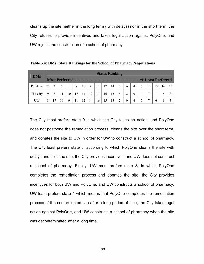
127
cleans up the site neither in the long term ( with delays) nor in the short term, the
City refuses to provide incentives and takes legal action against PolyOne, and
UW rejects the construction of a school of pharmacy.
Table 5.4: DMs’ State Rankings for the School of Pharmacy Negotiations
States Ranking DMs
Most Preferred ------------------------------------------------- Least Preferred PolyOne 2 3 5 1 8 10 9 11 17 14 0 6 4 7 12 13 16 15
The City 9 8 11 10 17 14 12 13 16 15 5 2 0 4 7 1 6 3
UW 8 17 10 9 11 12 14 16 15 13 2 0 4 5 7 6 1 3
The City most prefers state 9 in which the City takes no action, and PolyOne
does not postpone the remediation process, cleans the site over the short term,
and donates the site to UW in order for UW to construct a school of pharmacy.
The City least prefers state 3, according to which PolyOne cleans the site with
delays and sells the site, the City provides incentives, and UW does not construct
a school of pharmacy. Finally, UW most prefers state 8, in which PolyOne
completes the remediation process and donates the site, the City provides
incentives for both UW and PolyOne, and UW constructs a school of pharmacy.
UW least prefers state 4 which means that PolyOne completes the remediation
process of the contaminated site after a long period of time, the City takes legal
action against PolyOne, and UW constructs a school of pharmacy when the site
was decontaminated after a long time.
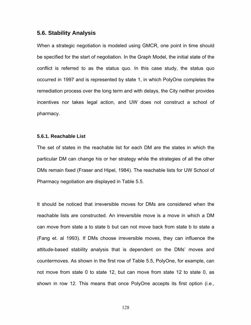
128
5.6. Stability Analysis
When a strategic negotiation is modeled using GMCR, one point in time should
be specified for the start of negotiation. In the Graph Model, the initial state of the
conflict is referred to as the status quo. In this case study, the status quo
occurred in 1997 and is represented by state 1, in which PolyOne completes the
remediation process over the long term and with delays, the City neither provides
incentives nor takes legal action, and UW does not construct a school of
pharmacy.
5.6.1. Reachable List
The set of states in the reachable list for each DM are the states in which the
particular DM can change his or her strategy while the strategies of all the other
DMs remain fixed (Fraser and Hipel, 1984). The reachable lists for UW School of
Pharmacy negotiation are displayed in Table 5.5.
It should be noticed that irreversible moves for DMs are considered when the
reachable lists are constructed. An irreversible move is a move in which a DM
can move from state a to state b but can not move back from state b to state a
(Fang et. al 1993). If DMs choose irreversible moves, they can influence the
attitude-based stability analysis that is dependent on the DMs’ moves and
countermoves. As shown in the first row of Table 5.5, PolyOne, for example, can
not move from state 0 to state 12, but can move from state 12 to state 0, as
shown in row 12. This means that once PolyOne accepts its first option (i.e.,
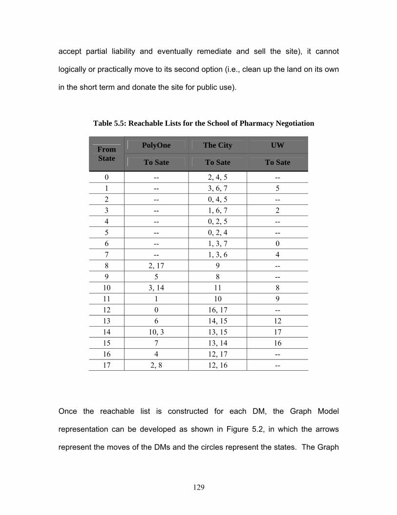
129
accept partial liability and eventually remediate and sell the site), it cannot
logically or practically move to its second option (i.e., clean up the land on its own
in the short term and donate the site for public use).
Table 5.5: Reachable Lists for the School of Pharmacy Negotiation
PolyOne The City UW From State To Sate To Sate To Sate
0 -- 2, 4, 5 -- 1 -- 3, 6, 7 5 2 -- 0, 4, 5 -- 3 -- 1, 6, 7 2 4 -- 0, 2, 5 -- 5 -- 0, 2, 4 -- 6 -- 1, 3, 7 0 7 -- 1, 3, 6 4 8 2, 17 9 -- 9 5 8 -- 10 3, 14 11 8 11 1 10 9 12 0 16, 17 -- 13 6 14, 15 12 14 10, 3 13, 15 17 15 7 13, 14 16 16 4 12, 17 -- 17 2, 8 12, 16 --
Once the reachable list is constructed for each DM, the Graph Model
representation can be developed as shown in Figure 5.2, in which the arrows
represent the moves of the DMs and the circles represent the states. The Graph
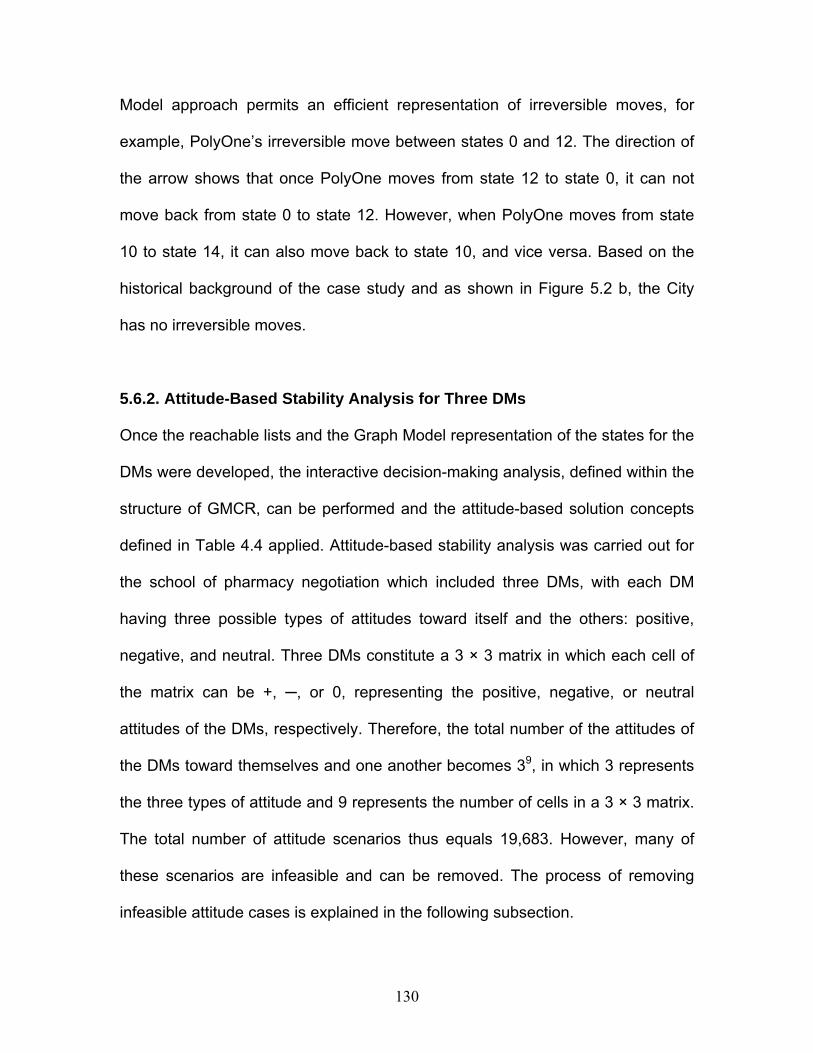
130
Model approach permits an efficient representation of irreversible moves, for
example, PolyOne’s irreversible move between states 0 and 12. The direction of
the arrow shows that once PolyOne moves from state 12 to state 0, it can not
move back from state 0 to state 12. However, when PolyOne moves from state
10 to state 14, it can also move back to state 10, and vice versa. Based on the
historical background of the case study and as shown in Figure 5.2 b, the City
has no irreversible moves.
5.6.2. Attitude-Based Stability Analysis for Three DMs
Once the reachable lists and the Graph Model representation of the states for the
DMs were developed, the interactive decision-making analysis, defined within the
structure of GMCR, can be performed and the attitude-based solution concepts
defined in Table 4.4 applied. Attitude-based stability analysis was carried out for
the school of pharmacy negotiation which included three DMs, with each DM
having three possible types of attitudes toward itself and the others: positive,
negative, and neutral. Three DMs constitute a 3 × 3 matrix in which each cell of
the matrix can be +, ─, or 0, representing the positive, negative, or neutral
attitudes of the DMs, respectively. Therefore, the total number of the attitudes of
the DMs toward themselves and one another becomes 39, in which 3 represents
the three types of attitude and 9 represents the number of cells in a 3 × 3 matrix.
The total number of attitude scenarios thus equals 19,683. However, many of
these scenarios are infeasible and can be removed. The process of removing
infeasible attitude cases is explained in the following subsection.
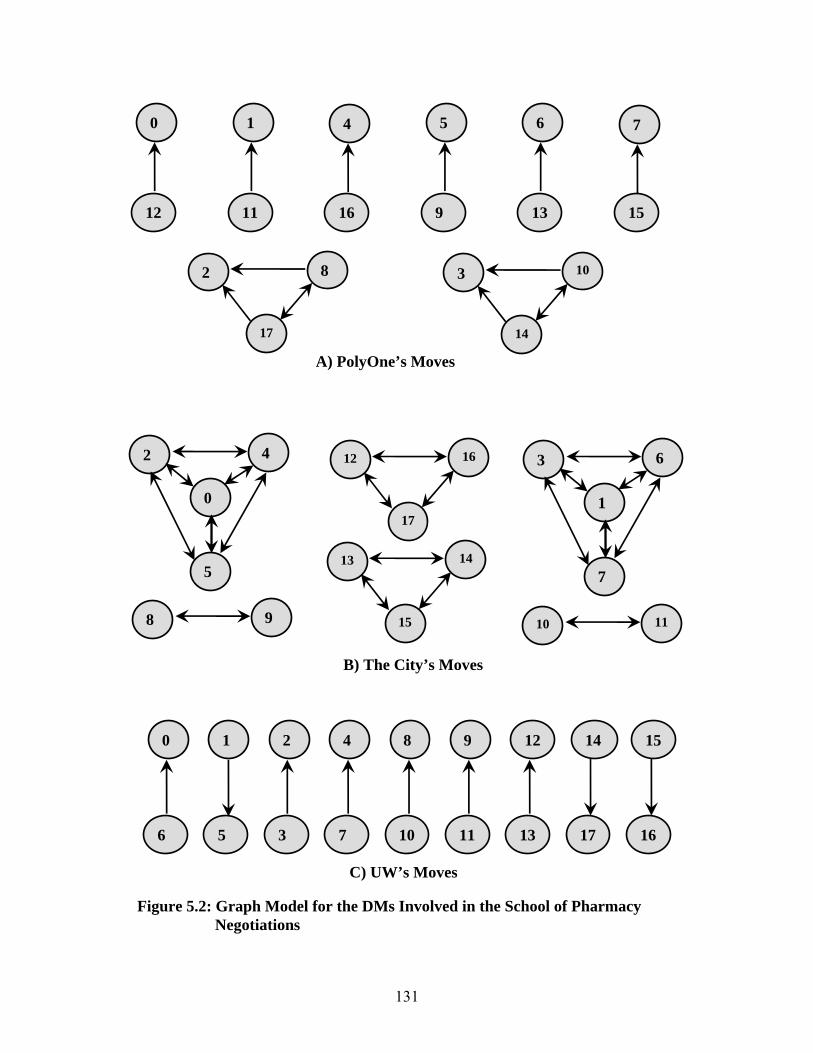
131
0
12
C) UW’s Moves
1
11
4
16
5
9
6
13
7
15
A) PolyOne’s Moves
17
2 8
14
3 10
0
2
5
4
1
3
7
6
15
13 14
17
12 16
B) The City’s Moves
8 9 10 11
0
6
2
3
8
10
12
13
14
17
15
16
1
5
4
7
9
11
Figure 5.2: Graph Model for the DMs Involved in the School of Pharmacy Negotiations
132
5.6.3. Proposed Algorithms for Removing Infeasible Attitude Cases
During negotiation, DMs may have a variety of attitudes toward themselves and
one another. Each attitude case corresponds to a situation in which the DMs
involved in the negotiations have one specific type of attitude (e.g., negative or
positive) toward themselves and one specific type of attitude (e.g., negative or
positive) toward other DMs. Among the total set of attitude cases, there are
always many attitude cases that cannot be taken into account and they are
referred to as infeasible attitude cases. Removing infeasible attitude cases
depends primarily on the real negotiation process. A negotiator in a negotiation
process may exhibit a variety of behaviors toward other negotiators. Inohara et
al. (2008) assumed that positive, negative, and neutral attitudes of a DM toward
others derive from “altruistic,” “sadistic,” and “apathetic” behaviors, respectively,
and those toward her/himself derive from “selfish,” “masochistic,” and “selfless”
behaviors, respectively, as shown in Table 4.2. Darling and Mumpower (1990)
identified eight strategic behavioral orientations for negotiators: 1) individualistic,
2) cooperative, 3) altruistic, 4) sacrificing, 5) self-destructive, 6) nihilistic, 7)
punitive, and 8) competitive, as shown in Figure 5.3. While such orientations are
uncommon and may sometimes be pathological, under specific circumstances
they may be useful concepts for achieving the broader purposes of negotiators.
The essence of the proposed algorithm for removing infeasible attitude cases is
based on the logic that DMs involved in construction negotiations cannot have
negative attitudes toward themselves. Therefore, all attitude cases in which a DM
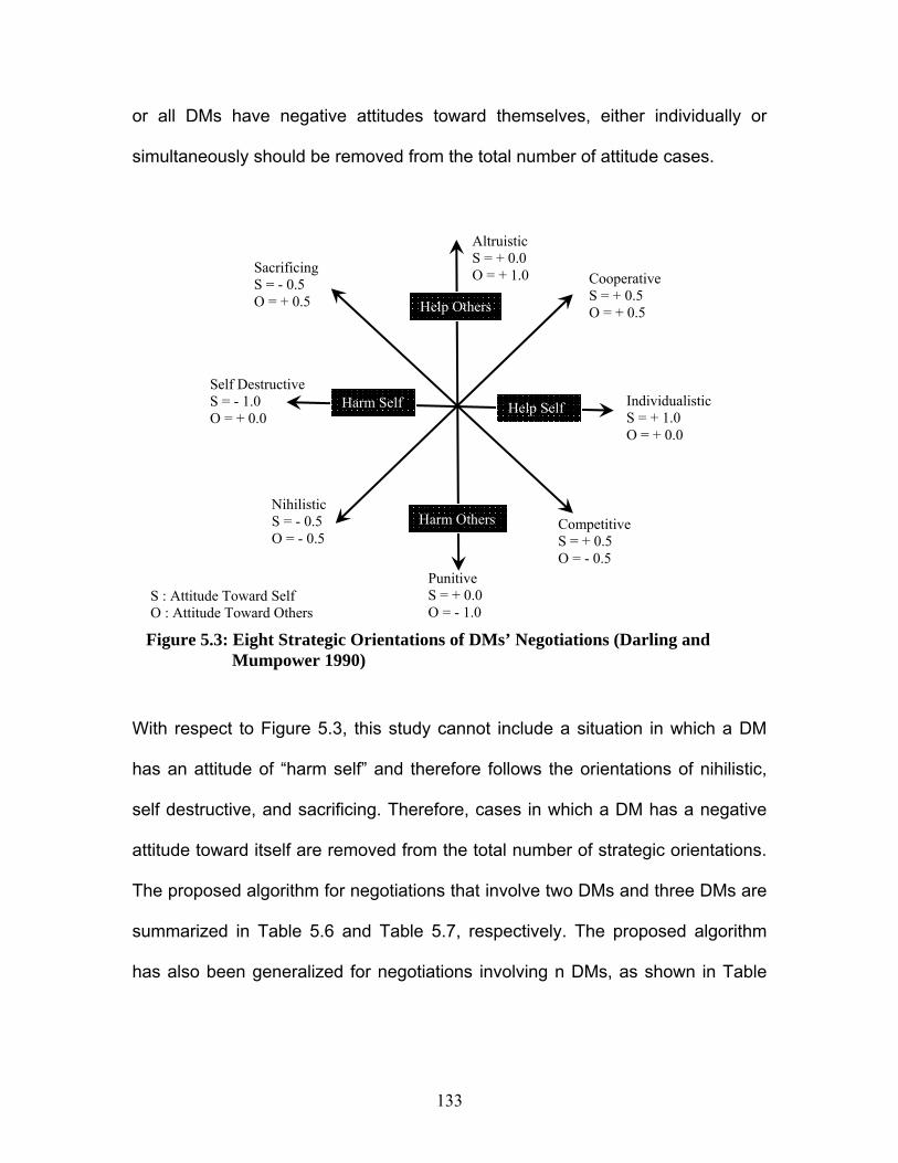
133
or all DMs have negative attitudes toward themselves, either individually or
simultaneously should be removed from the total number of attitude cases.
With respect to Figure 5.3, this study cannot include a situation in which a DM
has an attitude of “harm self” and therefore follows the orientations of nihilistic,
self destructive, and sacrificing. Therefore, cases in which a DM has a negative
attitude toward itself are removed from the total number of strategic orientations.
The proposed algorithm for negotiations that involve two DMs and three DMs are
summarized in Table 5.6 and Table 5.7, respectively. The proposed algorithm
has also been generalized for negotiations involving n DMs, as shown in Table
Nihilistic S = - 0.5 O = - 0.5
Self Destructive S = - 1.0 O = + 0.0
Sacrificing S = - 0.5 O = + 0.5
Cooperative S = + 0.5 O = + 0.5
Competitive S = + 0.5 O = - 0.5
Individualistic S = + 1.0 O = + 0.0
Punitive S = + 0.0 O = - 1.0
Harm Self
Help Others
Help Self
Harm Others
Altruistic S = + 0.0 O = + 1.0
S : Attitude Toward Self O : Attitude Toward Others
Figure 5.3: Eight Strategic Orientations of DMs’ Negotiations (Darling and Mumpower 1990)

134
5.8. The computer programming codes for these algorithms are provided in
Appendix A.
Table 5.6: Algorithm for Removing Infeasible Attitude Cases in Negotiations with
Two DMs Step Infeasible Matrix Description Infeasible Cases
1
DM1 DM2
DM1 ─
DM2 + or 0
Remove all cases in which DM1 has negative attitudes toward itself and DM2 has only neutral and positive attitudes toward itself, no matter what attitudes the DMs have toward each other.
1×3×3×2=18
2
DM1 DM2
DM1 + or 0
DM2 ─
Remove all cases in which DM2 has negative attitudes toward itself and DM1 has only neutral and positive attitudes toward itself, no matter what attitudes the DMs have toward each other.
2×3×3×1=18
3
DM1 DM2
DM1 ─
DM2 ─
Remove all cases in which DM1 has negative attitudes toward itself and DM2 has negative attitudes toward itself, no matter what attitudes the DMs have toward each other.
1×3×3×1=9
4 Total Number of Infeasible Attitude Cases 18+18+9 = 45 5 Total Number of Attitude Cases 3^4 = 81 6 Total Number of Feasible Attitude Cases 81 – 45 = 36
Table 5.7: Algorithm for Removing Infeasible Attitude Cases in Negotiations with
Three DMs
Step Infeasible Matrix Description Number of Infeasible Cases
1
DM1 DM2 DM3
DM1 ─
DM2 + or 0
DM3 + or 0
Remove all cases in which DM1 has negative attitudes toward itself and DM2 and DM3 have only neutral and positive attitudes toward themselves, no matter what attitudes the DMs have toward each other.
1×3×3×3×2×3×3×3×2=2916
2
DM1 DM2 DM3
DM1 + or 0
DM2 ─
DM3 + or 0
Remove all cases in which DM2 has negative attitudes toward itself and DM1 and DM3 have only neutral and positive attitudes toward themselves, no matter what attitudes the DMs have toward each other.
2×3×3×3×1×3×3×3×2=2916

135
3
DM1 DM2 DM3
DM1 + or 0
DM2 + or 0
DM3 ─
Remove all cases in which DM3 has negative attitudes toward itself and DM1 and DM2 have only neutral and positive attitudes toward themselves, no matter what attitudes the DMs have toward each other.
2×3×3×3×2×3×3×3×1=2916
4
DM1 DM2 DM3
DM1 ─
DM2 ─
DM3 + or 0
Remove all cases in which DM1 and DM2 have negative attitudes toward themselves and DM3 has only neutral and positive attitudes toward itself, no matter what attitudes the DMs have toward each other.
1×3×3×3×1×3×3×3×2=1458
5
DM1 DM2 DM3
DM1 ─
DM2 + or 0
DM3 ─
Remove all cases in which DM1 and DM3 have negative attitudes toward themselves and DM2 has only neutral and positive attitudes toward itself, no matter what attitudes the DMs have toward each other.
1×3×3×3×2×3×3×3×1=1458
6
DM1 DM2 DM3
DM1 + or 0
DM2 ─
DM3 ─
Remove all cases in which DM2 and DM3 have negative attitudes toward themselves and DM1 has only neutral and positive attitudes toward itself, no matter what attitudes the DMs have toward each other.
2×3×3×3×1×3×3×3×1=1458
7
DM1 DM2 DM3
DM1 ─
DM2 ─
DM3 ─
Remove all cases in which DM1, DM2, and DM3 have negative attitudes toward themselves, no matter what attitudes the DMs have toward each other.
1×3×3×3×1×3×3×3×1=729
4 Total Number of Infeasible Attitude Cases 13851 5 Total Number of Attitude Cases 3^9 = 19683 6 Total Number of Feasible Attitude Cases 19683 – 13851 = 5832
5.6.4. Determining the Most Relevant Feasible Attitude Cases
The proposed algorithms summarized in Tables 5.6 and 5.7 help a conflict
analyst remove a considerable number of infeasible attitude cases so that only
feasible attitude cases are considered. However, the remaining number of
feasible attitude cases is still too large to be evaluated using stability analysis.
Moreover, when the number of DMs increases, the resulting number of feasible
attitude cases increases exponentially, as shown in Tables 5.6 and 5.7.
Table 5.7: Cont.
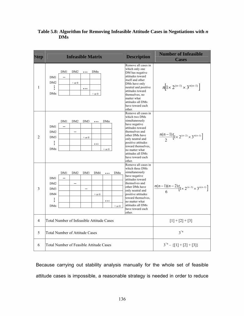
136
Table 5.8: Algorithm for Removing Infeasible Attitude Cases in Negotiations with n DMs
Because carrying out stability analysis manually for the whole set of feasible
attitude cases is impossible, a reasonable strategy is needed in order to reduce
Step Infeasible Matrix Description Number of Infeasible Cases
1
DM1 DM2 … DMn
DM1 ─
DM2 + or 0
…
…
DMn + or 0
Remove all cases in which only one DM has negative attitudes toward itself and other DMs have only neutral and positive attitudes toward themselves, no matter what attitudes all DMs have toward each other.
[ ])1()1( 321 −− ×× nnnn
2
DM1 DM2 DM3 … DMn
DM1 ─
DM2 ─
DM3 + or 0
…
…
DMn + or 0
Remove all cases in which two DMs simultaneously have negative attitudes toward themselves and other DMs have only neutral and positive attitudes toward themselves, no matter what attitudes all DMs have toward each other.
[ ])1()2( 3212
)1( −− ××− nnnnn
3
DM1 DM2 DM3 DM4 … DMn
DM1 ─
DM2 ─
DM3 ─
DM4 + or 0
…
…
DMn + or 0
Remove all cases in which three DMs simultaneously have negative attitudes toward themselves and other DMs have only neutral and positive attitudes toward themselves, no matter what attitudes all DMs have toward each other.
[ ])1()3( 3216
)2)(1( −− ××−− nnnnnn
4 Total Number of Infeasible Attitude Cases [1] + [2] + [3]
5 Total Number of Attitude Cases 3^n
6 Total Number of Feasible Attitude Cases 3^n – {[1] + [2] + [3]}

137
the number of feasible attitude cases. One such strategy is to select only the
feasible attitude cases that are most relevant to the negotiation situation under
investigation. In other words, determining the most relevant attitude cases
depends on each specific negotiation situation and how the DMs involved are
expected to behave before and during the negotiation. This strategy helps the
analyst focus on a small number of attitude cases with the highest degree of
relevance so that going through the whole set of feasible cases is unnecessary.
With respect to the brownfield negotiation case study, the historical background
was reviewed and the attitudes of the three DMs toward one another were
studied. A list of the six most relevant attitude cases was then determined, and
these six cases were examined using attitude-based stability analysis. The six
attitude cases and a brief description of each are listed in Table 5.9.
5.6.5. Analysis of the Most Relevant Attitude Cases
Once the six most relevant attitude cases were selected, the stability analysis
within the paradigm of GMCR was carried out in order to obtain equilibrium
states or possible solutions for the conflict. A separate attitude-based stability
analysis was carried out for each of the six attitude cases selected, as shown in
the stability tableaus displayed in Figures 5.4, 5.5, 5.6, 5.7, 5.8, and 5.9. It is
noted that the tableaus used in the conventional GMCR were expanded in order
to include the attitude based stability analysis.
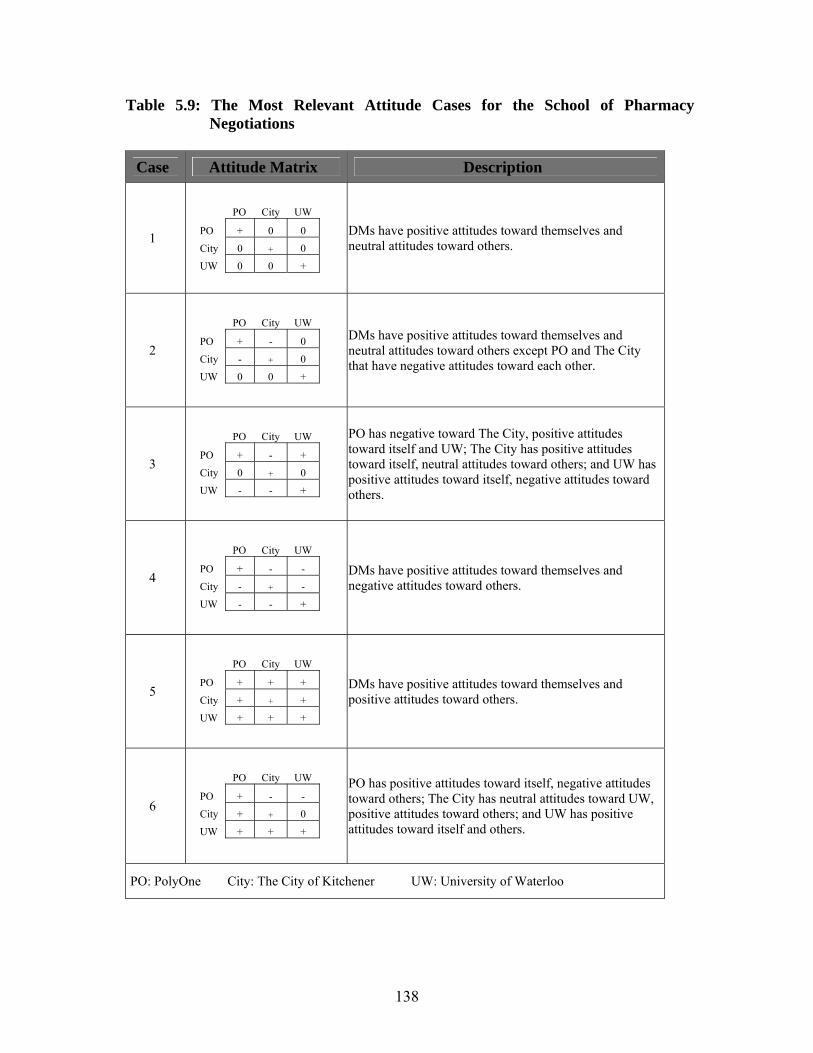
138
Table 5.9: The Most Relevant Attitude Cases for the School of Pharmacy Negotiations
Case Attitude Matrix Description
1
PO City UW
PO + 0 0
City 0 + 0
UW 0 0 +
DMs have positive attitudes toward themselves and neutral attitudes toward others.
2
PO City UW
PO + - 0
City - + 0
UW 0 0 +
DMs have positive attitudes toward themselves and neutral attitudes toward others except PO and The City that have negative attitudes toward each other.
3
PO City UW
PO + - +
City 0 + 0
UW - - +
PO has negative toward The City, positive attitudes toward itself and UW; The City has positive attitudes toward itself, neutral attitudes toward others; and UW has positive attitudes toward itself, negative attitudes toward others.
4
PO City UW
PO + - -
City - + -
UW - - +
DMs have positive attitudes toward themselves and negative attitudes toward others.
5
PO City UW
PO + + +
City + + +
UW + + +
DMs have positive attitudes toward themselves and positive attitudes toward others.
6
PO City UW
PO + - -
City + + 0
UW + + +
PO has positive attitudes toward itself, negative attitudes toward others; The City has neutral attitudes toward UW, positive attitudes toward others; and UW has positive attitudes toward itself and others.
PO: PolyOne City: The City of Kitchener UW: University of Waterloo

139
Figure 5.4: Stability Tableau for Case 1
Figure 5.5: Stability Tableau for Case 2
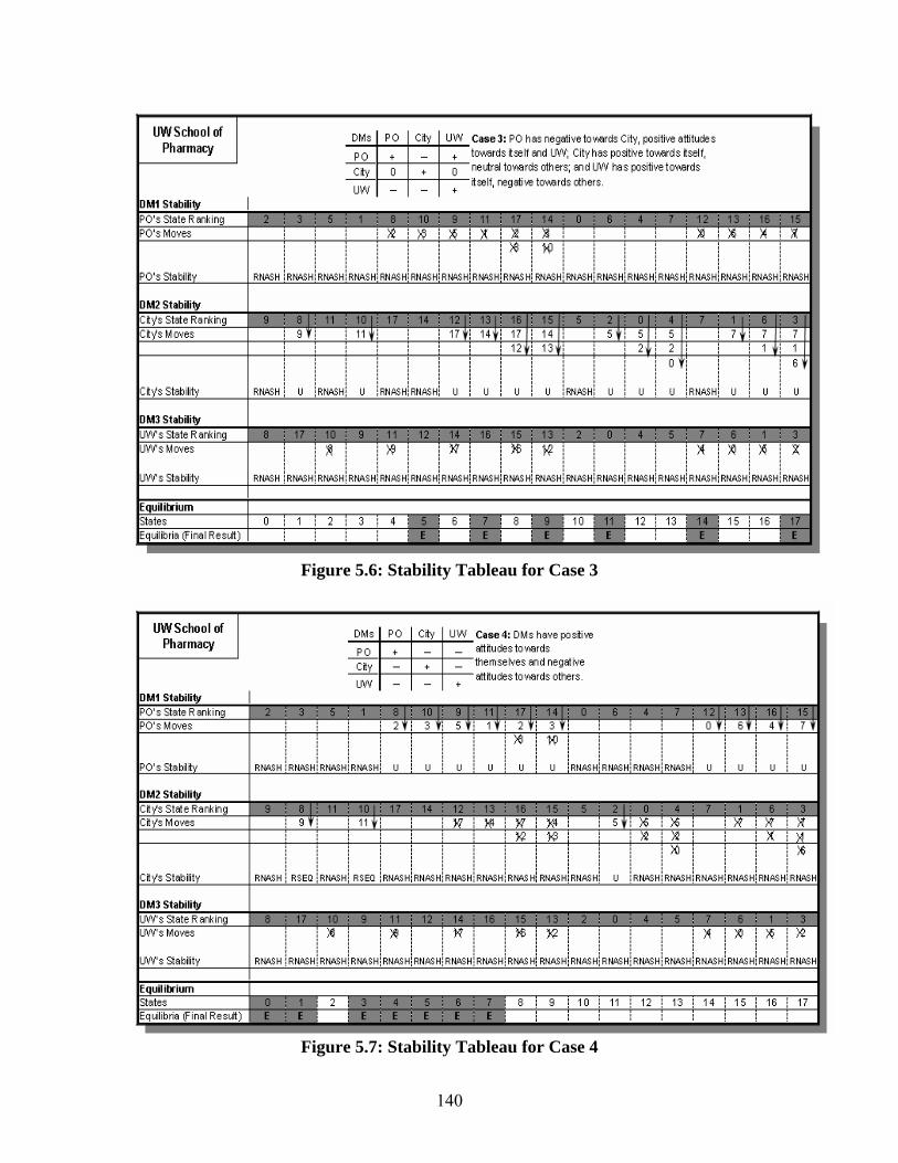
140
Figure 5.6: Stability Tableau for Case 3
Figure 5.7: Stability Tableau for Case 4
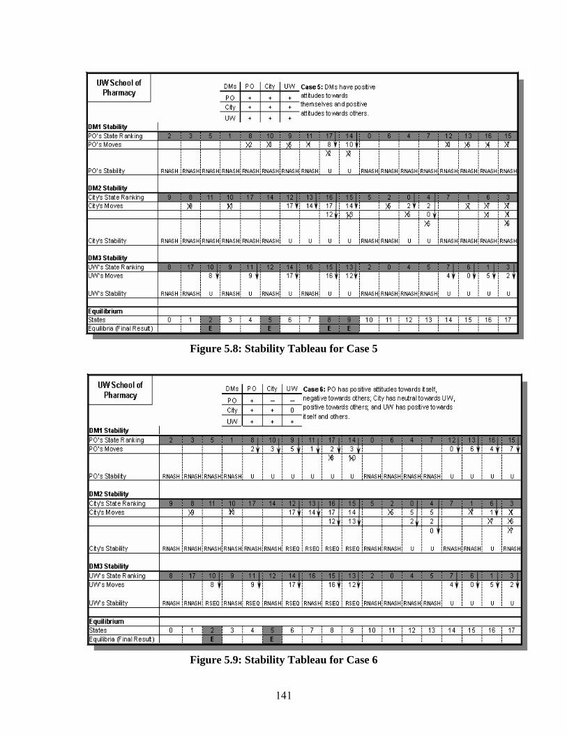
141
Figure 5.8: Stability Tableau for Case 5
Figure 5.9: Stability Tableau for Case 6

142
5.7. Discussion of the Results of the Stability Analyses
As shown in Figures 5.4 – 5.9, because of the changes in the attitudes of the
DMs, six different sets of equilibrium states were obtained, corresponding to the
six different attitude cases. The equilibrium states involved in each attitude case
represent possible strategic solutions for the multi-DM negotiations. These six
sets of resulting decision options were then evaluated in order to determine the
best strategic decision. The resulting equilibrium states are shown in Figure 5.10,
and a brief discussion of each case follows.
Equilibrium States Case 1: DMs PO City UW PO + 0 0 10 11 City 0 + 0
UW 0 0 + Case 2: DMs PO City UW PO + ─ 0 0 4 10 11 14 City ─ + 0
UW 0 0 + Case 3: DMs PO City UW PO + ─ + 7 9 11 14 17 City 0 + 0 UW ─ ─ +
Case 4: DMs PO City UW PO + ─ ─ 0 1 3 4 6 7 City ─ + ─ UW ─ ─ +
Case 5: DMs PO City UW PO + + + 2 8 9 City + + +
UW + + + Case 6: DMs PO City UW PO + ─ ─ 2 City + + 0 UW + + +
Figure 5.10: The Results of the Stability Analysis for the Six Attitude Cases
Stability Analysis
Stability Analysis
Stability Analysis
Stability Analysis
Stability Analysis
Stability Analysis

143
It should be mentioned that of the 14 resulting equilibrium states, equilibrium
state 5 is a false equilibrium and is not listed in Figure 5.10 because state 5 is the
only state that remained RNASH stable for all DMs and in all attitude cases
(Fraser and Hipel, 1984). In other words, state 5 is the only state in which the
involved DMs can not find one move from that state to other states in the six
attitude cases investigated above. Moreover, status quo analysis shows that
state 5 can not be an equilibrium state (Li et al., 2004). Status quo analysis
addresses concerns about the reachability of any specified state from the status
quo. Since the Graph Model introduces the notion of irreversible moves (DMs
can cause the conflict to move in one direction but not the other) to reflect no-
return decisions, the reachability of a state from a status quo is not automatically
guaranteed. If some of the moves are specified as irreversible at the modeling
stage, it is possible that some of the predicted resolutions cannot be attained
from the status quo state, and an analyst may safely eliminate such states (e.g.,
equilibrium state 5) from the potential resolution list and concentrate on a refined
list (Li et al., 2004).
5.7.1. Qualitative Analysis of the Findings
Case 1: Figure 5.4 displays a scenario in which the DMs have positive attitudes
toward themselves and neutral attitudes toward other DMs. The stability analysis
was carried out, and outcomes (i.e., equilibrium states) 10 and 11 resulted for
this case. Outcome 10 is more preferred to outcome 11 for PolyOne and UW.
Also, outcome 11 is more preferred to outcome 10 for the city. Outcome 10

144
means that PolyOne (PO) cleans up the property in the short term (fast), UW
refuses to construct a school of pharmacy in the remediated site, and the City
does not take legal action against PO and provides incentives for both PO and
UW. Outcome 11 means that PO cleans up the land quickly, the City neither
takes legal action nor provides incentives, and UW does not construct a school of
pharmacy on the site. It should be mentioned that an attitude case (i.e., case 0)
was considered in which the DMs have neutral attitudes towards themselves and
towards other DMs. When such attitude case was considered, the same
individual stability and equilibrium results, as for case 1, were obtained.
Case 2: Figure 5.5 shows another attitude case in which the DMs have positive
attitudes toward themselves and neutral attitudes toward others except for PO
and the City who have negative attitudes toward each other. In this attitude case,
the resulting set of possible solutions includes outcomes 0, 4, 10, 11, and 14. A
comparison of the sets of outcomes for Case 1 and Case 2 (Figure 5.10)
indicates that Case 2 is identical to Case 1, except that the set of solutions also
includes outcomes 0 and 4. Considering the DMs’ state rankings, it can be seen
that of the set of outcomes in Case 2, outcomes 0 and 4 are the least preferred
for all DMs. Outcome 4, for example, means that PO cleans up the land over the
long term (slow), the City does not provide incentives and takes legal action
against PO, and UW constructs a school of pharmacy without any incentives. It
can be concluded that because two DMs (i.e., PO and the City) have negative
attitudes toward each other, the set of possible solutions in Case 2 has been

145
shifted to the right side of the DMs’ state rankings which represent states that are
less preferred by the DMs.
Case 3: Figure 5.6 shows the attitude scenario that occurs when PO has a
negative attitude toward the City, a positive attitude toward itself and UW; the
City has a positive attitude toward itself, a neutral attitude toward the others; and
UW has a positive attitude toward itself, and a negative attitude toward the
others. This attitude scenario examines a situation in which the attitudes of the
DMs toward one another are not consistent. In other words, while DM 1 has a
negative attitude toward DM 2, it is possible that DM 2 has a positive attitude
toward DM 1. For example, PO has a negative attitude toward the City; whereas
the City has a neutral attitude toward PO, as shown in Figure 5.6. In addition,
when UW has a negative attitude toward the others, PO and the City have
positive and neutral attitudes toward UW, respectively. The resulting set of
possible solutions for Case 3 includes outcomes 7, 9, 11, 14, and 17. According
to the DMs’ state rankings, some of the outcomes are less preferred and some
are more preferred so that no single outcome is the most beneficial for all DMs. A
comparison of the sets of outcomes in Cases 2 and 3 shows that outcome 7
appears in Case 3, in which the DMs have more hostile attitudes toward one
another than in Case 2 (i.e., Case 2 has two negative symbols (─) in its attitude
matrix, whereas Case 3 has three negative symbols (─) in its attitude matrix, as
shown in Figures 5.5 and 5.6, respectively). Outcome 7 is also the only outcome
that is the least beneficial outcome for all DMs. Outcome 7 means that PO cleans
up the land, the City does not provide incentives and takes legal action against
146
PO, and UW does not construct a school of pharmacy. The reason that this
outcome is the least preferred can be explained by the legal action taken by the
City. In other words, the DMs least prefer the costly and lengthy litigation
involved in taking a conflict case to court. It can be concluded from this attitude
scenario that because of the inconsistency in the attitudes of the DMs toward one
another, a less coherent set of outcomes is obtained, and as a result, some
outcomes are shifted to the left side (more preferred) and some outcomes are
shifted to the right side (less preferred) of the DMs’ state rankings. In this case, it
is very hard for an analyst to provide a single beneficial solution for the DMs
involved in the strategic negotiations.
Case 4: Figure 5.7 shows an attitude scenario in which the DMs have a positive
attitude toward themselves and a negative attitude toward the other DMs. This
case represents the most hostile attitude scenario in which all the DMs involved
have negative attitudes toward one another. The resulting set of outcomes for
this attitude scenario consists of outcomes 0, 1, 3, 4, 6, and 7. A comparison of
the six sets of outcomes, which correspond to the six attitude cases, indicates
that the set of outcomes in Case 4 is the worst set of outcomes resulting from the
attitude-based stability analysis. In other words, considering the DMs’ state
rankings, the resulting outcomes have been shifted substantially to the left side of
the state ranking for each DM. For example, outcome 3 is the least preferred
state in the state rankings of the City and UW (Table 5.10). Moreover, outcomes
0, 4, 6, and 7 include a situation in which the City takes legal action, which is the
147
least preferred action for all the DMs. It can be concluded that when the DMs
involved in the strategic negotiations possess a negative attitude toward one
another, the resulting outcomes represent the least beneficial decisions for the
DMs involved.
Case 5: Figure 5.8 shows an attitude scenario in which the DMs have a positive
attitude toward themselves and a positive attitude toward one another: the
opposite of the previous case (Case 4) in which the DMs have a negative attitude
toward one another. The stability analysis for case 5 results in a set of outcomes
2, 8, and 9. This set is shifted to the far left side of the DMs’ state rankings and
are therefore more preferred by the DMs. With such an attitude scenario,
outcome 8, for example, is the most preferred outcome for UW, the second most
preferred outcome for the city, and the fifth most preferred outcome for PO.
Outcome 8 means that PO cleans up the land fast, the city does not take legal
action against PO and provides incentives for PO and UW, and UW constructs a
school of pharmacy on the decontaminated site. It can be concluded that, in
multi-DMs brownfield negotiations, when the DMs possess positive attitudes
toward one another, more beneficial outcomes result and the DMs have a better
opportunity to agree on one outcome at the strategic level and then continue with
detailed negotiations at the tactical level. It should be mentioned that if the level
of information indicates that the DMs indeed have positive attitudes toward one
another, outcome 8 can be considered as potential final solution to the

148
negotiations at the strategic level. Further discussion has been provided in
Subsection 5.7.2.
Case 6: Figure 5.9 shows an attitude scenario in which PO has a positive attitude
toward itself and a negative attitude toward the others, the city has a neutral
attitude toward UW and a positive attitude toward itself and PO, and UW has a
positive attitude toward itself and the others. This attitude scenario examines how
the outcome of the negotiation changes when a DM (e.g., PO) that has a
negative attitude negotiates with the other DMs (e.g., the City and UW) that have
a positive attitude. The resulting set of outcomes is limited to outcome 2.
Considering the DMs’ state rankings, it can be observed that outcome 2 is more
preferred by PO and less preferred by the City and UW and that, it is very difficult
the DMs involved to reach mutual agreement with this attitude case. It can be
concluded that when DM 1 has a negative attitude toward DM 2 and DM 3, but
DM 2 and DM 3 have a positive attitude toward DM 1, only a few outcomes can
be resulted from negotiations, and the outcomes mostly benefit DM 1. There is
also a low likelihood that the DMs will agree on one outcome as a possible
solution.
The qualitative analysis of the above six attitude cases indicates that the
resulting outcomes in case 4 are more hostile for all DMs and may therefore be
less preferred. On the other hand, the resulting outcomes in case 5 are more
beneficial for all DMs and may therefore be more preferred if the level of
149
negotiation information is sufficient to indicate that all DMs involved indeed have
had positive attitudes toward one another. As well, of the 14 resulting equilibrium
outcomes, some are repeated in some of the attitude cases. For example,
outcome 11 resulted in cases 1, 2, and 3. As mentioned in Chapter 4, the
frequency with which a state becomes a possible solution in different attitude
cases may indicate that the state is a stable state and that no matter how the
attitudes of the DMs change, the stable state can still result as an equilibrium
state (outcome). As a result, the likelihood of such stable states becoming the
best strategic outcome of the negotiations is increased. It should be noted,
however, that the attitudes of the DMs can significantly influence the final
outcome of the strategic negotiations. Therefore, to assess the impact of the
DMs’ attitudes on the choice of the final strategic solution, a quantitative analysis
was conducted, as explained in the following subsection.
5.7.2. Quantitative Analysis of the Findings
Qualitative analysis of the resulting equilibrium states is a common procedure in
the conventional GMCR. However, when the number of resulting equilibrium
states is increased, it is cumbersome to qualitatively recommend one possible
solution to the conflict. Therefore, to support the qualitative analysis of the
stability results discussed in the previous subsection, quantitative analysis was
also conducted for the brownfield case study negotiations as an ad hoc analysis.
The objective was to provide quantitative measures 1) to show how different
types of DMs’ attitudes can influence their level of satisfaction with the

150
multilateral negotiations conducted in the case study and 2) to provide a
complementary tool for the qualitative approach in order to determine the most
beneficial strategic decision resulting from the negotiation. To achieve these
objectives, attitude case 6 (Figure 5.10), for example, was considered and the
quantitative analysis was carried out using the proposed framework shown in
Figure 5.11. The following steps were involved in developing the quantitative
approach.
Figure 5.11: The Proposed Framework for the Quantitative Analysis
5.7.2.1. Step 1: Determine the attitude values
In each attitude case, the DMs possess positive, neutral, or negative attitudes
toward themselves and one another. In the proposed approach, the qualitative
attitudes (i.e., positive, neutral, and negative) are transferred to quantitative
Step 1
DMs PO City UW Sum of Attitude
PO + ? ? -0.33
City + + 0 0.67
UW + + + 1
Step 3
Draw the attitude-satisfaction graph
Step 2
42
State 2
100
36
42
DM's Satisfaction in Equilb. States (%)
100
36
Average Satisfaction
(%)
Determine the average satisfaction values
Determine the attitude values for each attitude case
(e.g., 6)
PO
CityUW
0
20
40
60
80
100
120
-0.33 0.67 1.00Attitude (Step 1)
Satis
fact
ion
(Ste
p 2)
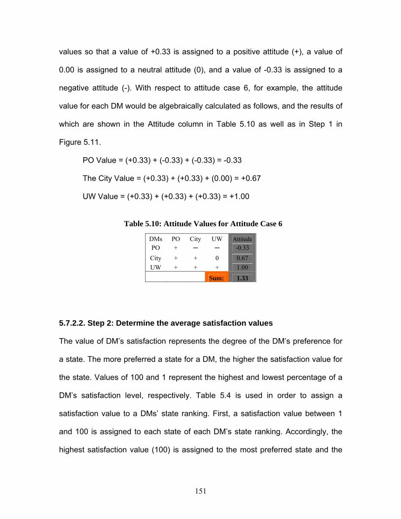
151
values so that a value of +0.33 is assigned to a positive attitude (+), a value of
0.00 is assigned to a neutral attitude (0), and a value of -0.33 is assigned to a
negative attitude (-). With respect to attitude case 6, for example, the attitude
value for each DM would be algebraically calculated as follows, and the results of
which are shown in the Attitude column in Table 5.10 as well as in Step 1 in
Figure 5.11.
PO Value = (+0.33) + (-0.33) + (-0.33) = -0.33
The City Value = (+0.33) + (+0.33) + (0.00) = +0.67
UW Value = (+0.33) + (+0.33) + (+0.33) = +1.00
Table 5.10: Attitude Values for Attitude Case 6
5.7.2.2. Step 2: Determine the average satisfaction values
The value of DM’s satisfaction represents the degree of the DM’s preference for
a state. The more preferred a state for a DM, the higher the satisfaction value for
the state. Values of 100 and 1 represent the highest and lowest percentage of a
DM’s satisfaction level, respectively. Table 5.4 is used in order to assign a
satisfaction value to a DMs’ state ranking. First, a satisfaction value between 1
and 100 is assigned to each state of each DM’s state ranking. Accordingly, the
highest satisfaction value (100) is assigned to the most preferred state and the
DMs PO City UW Attitude PO + ─ ─ -0.33 City + + 0 0.67 UW + + + 1.00 Sum: 1.33

152
lowest satisfaction value (1) is assigned to the least preferred state, with other
values at a decreasing rate of 100/17 being assigned to the rest of states from
left to right for each DM, as shown in Table 5.11. It is assumed in this situation
that there is a fixed rate of satisfaction between the two adjacent states with
respect to all of the DMs. As an alternative approach, it would be possible to
assign different satisfaction values to the states with a variable rate. Because of
the connection between a DM’s satisfaction and preference in this research, the
satisfaction value is sometimes referred to as the preference value when the
influence of the DMs’ attitudes is not considered.
Table 5.11: Satisfaction Values for States in the DMs’ State Rankings
Satisfaction and State Rankings DMs
Most Preferred -------------------------------------------------- Least Preferred
Satisfaction 100 94 88 83 77 71 65 59 53 48 42 36 30 24 18 12 7 1 PolyOne
State 2 3 5 1 8 10 9 11 17 14 0 6 4 7 12 13 16 15
Satisfaction 100 94 88 83 77 71 65 59 53 48 42 36 30 24 18 12 7 1 City
State 9 8 11 10 17 14 12 13 16 15 5 2 0 4 7 1 6 3
Satisfaction 100 94 88 83 77 71 65 59 53 48 42 36 30 24 18 12 7 1 UW
State 8 17 10 9 11 12 14 16 15 13 2 0 4 5 7 6 1 3
One of the benefits of Table 5.11 is that the average satisfaction value of the
equilibrium states (Figure 5.10) can be calculated for all DMs. Such a satisfaction
value is designated the combined average satisfaction value since the combined
satisfaction relates to all DMs. It should be remembered that the equilibrium
states constitute a subset of a DM’s state ranking. The average satisfaction value

153
for equilibrium states 6 and 8, for example, are calculated as shown in Table
5.12. It is assumed that the DMs have similar valuation for their satisfaction.
The same procedure is carried out in order to calculate the average satisfaction
value for the remaining equilibrium states, the results of which are shown in
Figure 5.12. It should be mentioned that the average satisfaction value is also
referred to as the combined satisfaction value since the value represents the
satisfaction level of all DMs.
Table 5.12: The Average Satisfaction Values for Equilibrium States 6 and 8
To facilitate a better understanding of the importance of this approach, the
equilibrium states are sorted based on their calculated average satisfaction
value. Accordingly, the values and states in Figure 5.12 are replaced and sorted
as shown in Figure 5.13. It should be noted that the results shown in Figures
5.12 and 5.13 do not reflect the influence of the attitudes of the DMs and that
these figures represent only a regular quantitative preference for the resulting
equilibrium states when the DMs equally prefer the states.
PO The City UW
Equilibrium 8 6 8 6 8 6
Satisfaction 77 36 94 7 100 13
Average Satisfaction for State 8
903
1009477=
++
Average Satisfaction for State 6
183
13736=
++
154
36 36
59
3228
18 20
9083 81
75
61
69
0
10
20
30
40
50
60
70
80
90
100
0 1 2 3 4 6 7 8 9 10 11 14 17
Equilibrium States (Outcomes)
Ave
rage
Sat
isfa
ctio
n (%
)
Figure 5.12: Combined Satisfaction Level of the Equilibrium States Disregarding the Influence of the DMs’ Attitudes
Equilibrium States (Outcomes)
9083 81
7569
61 59
36 3632
28
20 18
0
10
20
30
40
50
60
70
80
90
100
8 9 10 11 17 14 2 0 1 3 4 7 6
Aver
age
Sat
isfa
ctio
n (%
)
Figure 5.13: Sorted Satisfaction Level of the Equilibrium States Disregarding the Influence of the DMs’ Attitudes
155
Once a satisfaction value is assigned to every state, as shown in Table 5.11, the
equilibrium states for each attitude case are considered, and their satisfaction
values are calculated. In attitude case 6, for example, the resulting equilibrium
state is outcome 2. With respect to equilibrium state 2, satisfaction values of 100,
36, and 42 are determined for Polyone, the City, and UW, respectively. These
values are shown in Figure 5.11 (Step 2).
Once the satisfaction level for each equilibrium state has been determined, the
average satisfaction value for each DM in each attitude case can be calculated.
With respect to attitude case 6, for example, because there is only one
equilibrium state, the average satisfaction value for each DM is calculated to be
the same as its original value in the attitude case, as shown in Step 2 in Figure
5.11.
5.7.2.3. Step 3: Draw the attitude-satisfaction graph
Once the average satisfaction value is obtained for every DM, the attitude values
obtained in Step 1 and the average satisfaction values determined in Step 2 are
used to draw an attitude-satisfaction graph. This graph indicates how a DM’s
attitudes change his or her level of satisfaction and also helps the analyst
investigate the position of DMs with respect to every attitude case. In other
words, for an attitude-based negotiation involving multiple DMs, the graph shows
how much each DM gains when a particular attitude case (which represents the
DMs attitudes toward themselves and others) is considered. The attitude-
satisfaction graph for attitude case 6, for example, is displayed in Figure 5.14.

156
The graph shows that when PO possesses an overall negative attitude value of -
0.33, PO gains the highest level of satisfaction (100 %). On the other hand, when
UW has a very positive attitude (+1), its level of satisfaction reaches the lowest
value of 42 %. These results may indicate why attitude case 6 is very
encouraging for PO and very discouraging for UW. With respect to the City,
although the City’s overall attitude value is positive (+0.67), its level of
satisfaction is not so high (36 %) and the City may thus not prefer attitude case 6.
PO = 100
City = 36UW = 42
0.00
20.00
40.00
60.00
80.00
100.00
-0.3 0.0 0.3 0.7 1.0
Attitude Value
Satisfaction (%)
Figure 5.14: The Attitude-Satisfaction Graph for Attitude Case 6
The same quantitative procedure, as explained above for attitude case 6, was
carried out for the remaining five attitude cases. The resulting values and attitude
matrices are displayed in Table 5.13, and the resulting attitude-satisfaction
graphs are shown in Figures 5.15 and 5.16. A brief discussion of each attitude
case is also provided below.
157
Case 1: With respect to attitude case 1, the DMs involved have gained almost
the same satisfaction with the same positive attitude value (+0.33), as shown in
Figure 5.13. This type of attitude scenario is reasonable and encouraging for the
DMs since every DM gains almost equally and no DM loses. It should be noted
that the level of satisfaction of the DMs is also reasonable.
Table 5.13: Attitude and Satisfaction Values for Six Attitude Cases
Attitude Case 1 Attitude Case 2
DMs PO City UW DM’s
Attitude Ave. DM’s Satisfaction
PO + 0 0 0.33 59
City 0 + 0 0.33 81
UW 0 0 + 0.33 77
DMs PO City UW DM’s Attitude
Ave. DM’s Satisfaction
PO + ─ 0 0.00 50
City ─ + 0 0.00 59
UW 0 0 + 0.33 59
Attitude Case 3 Attitude Case 4
DMs PO City UW DM’s Attitude
Ave. DM’s Satisfaction
PO + ─ + 0.33 50
City 0 + 0 0.33 71
UW ─ ─ + -0.33 67
DMs PO City UW DM’s Attitude
Ave. DM’s Satisfaction
PO + ─ ─ -0.33 51
City ─ + ─ -0.33 16
UW ─ ─ + -0.33 18
Attitude Case 5 Attitude Case 6
DMs PO City UW DM’s Attitude
Ave. DM’s Satisfaction
PO + + + 1.00 81
City + + + 1.00 77
UW + + + 1.00 75
DMs PO City UW DM’s
Attitude Ave. DM’s Satisfaction
PO + ─ ─ -0.33 100
City + + 0 0.67 36
UW + + + 1 42
Case 2: In attitude case 2, UW and the City have achieved better level of
satisfaction because of UW’s positive attitude value. In this case PO and the City
have a negative attitude toward each other and PO’s overall gain is thus

158
diminished, whereas UW has gained because of its neutral attitude. In other
words, if the DMs possess a negative attitude toward other DMs, they may lose.
Attitude Case 1
Attitude Case 2
Attitude Case 4
Attitude Case 5
0
20
40
60
80
100
-0.33 0 0.33 0.66 0.99
Attitude
Satisfaction (%)
PO
City
UW
Area 1:HIGH SatisfactionLOW Attitude
Area 2:HIGH SatisfactionHIGH Attitude
Area 3:LOW SatisfactionHIGH Attitude
Area 4:LOW SatisfactionLOW Attitude
Figure 5.15: Attitude Satisfaction Relationship for Attitude Cases 1, 2, 4, and 5
Attitude Case 3
Attitude Case 6
0
20
40
60
80
100
-0.33 0 0.33 0.66 0.99Attitude
Satisfaction (%)
POCityUW
Area 1:HIGH SatisfactionLOW Attitude
Area 2:HIGH SatisfactionHIGH Attitude
Area 3:LOW SatisfactionHIGH Attitude
Area 4:LOW SatisfactionLOW Attitude
Figure 5.16: Attitude Satisfaction Relationship for Attitude Cases 3 and 6
159
It should be mentioned that to facilitate the analysis, Figures 5.15 and 5.16 are
divided into four distinct areas:
• Areas 1: low attitude value and high level of satisfaction,
• Area 2: high attitude value and high level of satisfaction,
• Area 3: high attitude value and low level of satisfaction, and
• Area 4: low attitude value and low level of satisfaction.
Case 3: In this case, the City has a neutral attitude toward the other DMs and
has therefore gained slightly more than PO and UW. The attitude situation in this
case indicates that PO has a positive attitude toward UW, whereas UW has a
negative attitude toward PO. In other words, the attitudes of the DMs toward one
another are not necessarily logical, and consequently, when UW, for example,
has a negative attitude value, its satisfaction level exceeds that of PO whose
attitude value is positive.
Case 4: This attitude case is the most hostile attitude scenario, in which the DMs
have a negative attitude toward one another and a positive attitude toward
themselves. The DMs’ attitude values are therefore similarly (-0.33). Interestingly,
the PO’s satisfaction level is much higher than the City’s and UW’s. This result
means that when the DMs negotiate in a hostile situation, PO can benefit, while
UW and the City may lose significantly. Although this situation may be beneficial
for PO, it is certainly not preferable for all the DMs involved.

160
Case 5: This case represents situation opposite to that in Case 4, in which the
DMs all have a positive attitude toward one another. Therefore, both their attitude
and their satisfaction level have reached the highest value (Figure 5.13).
Because all DMs gain almost equally and no DM loses, this situation is very
encouraging for DMs who are involved in cooperative negotiations.
Case 6: In this case, PO has a negative attitude toward the other DMs, whereas
UW has a positive attitude toward the other DMs. The result of negotiating in this
situation is that PO, who has the lowest attitude value (-0.33), has gained
significantly, and UW, who has the highest attitude value (+1), has lost
considerably, as shown in Figure 5.13. This situation is therefore very useful for
DMs who find out that other DMs in negotiations have a positive attitude toward
other DMs no matter how the other DMs’ attitudes may change during
negotiations.
5.7.3. Determining the Most Beneficial Strategic Decision
The results of the qualitative and quantitative analyses explained in the previous
subsections were used to determine which equilibrium state is the most
beneficial decision option in the multiple-DM brownfield negotiation. In
Subsection 5.7.2, the relationship between satisfaction level and the DM’s
attitude was described from each DM’s perspective. Six distinct attitude cases
were considered for each of which the satisfaction level of each individual DM
was discussed and compared with the levels of satisfaction for the other DMs. In

161
this subsection, the influence of a DM’s attitude on the level of satisfaction is
analyzed from the perspective of an analyst (e.g., a mediator). In other words, it
is assumed that an analyst examines the results regardless of the perspective of
each DM, and provides the DMs with advice that indicates the best outcome of
the negotiation at the strategic level.
To determine the best strategic solution, the equilibrium states are examined.
Table 5.14 shows the resulting values for the DMs’ attitude and level of
satisfaction and Figure 5.17 shows the six attitude cases represented by gray
column bars that list their corresponding equilibrium states. The upward arrow in
each column indicates for each attitude case the preference for the equilibrium
states, based on Figure 5.13. The dotted line in the graph represents continuous
changes and the gray columns represent the discrete changes in the combined
level of the DM’s satisfaction.
Table 5.14: Values of the DMs’ Attitude and Satisfaction
PO The City UW Attitude Case Attitude Satisfaction Attitude Satisfaction Attitude Satisfaction
Sum of DMs'
Attitudes Ave. DMs'
Satisfaction 1 0.33 59 0.33 81 0.33 77 1.00 72 2 0 50 0 59 0.33 59 0.33 56 3 0.33 50 0.33 71 -0.33 67 0.33 63 4 -0.33 51 -0.33 16 -0.33 18 -1.00 28 5 1 81 1 77 1 75 3.00 78 6 -0.33 100 0.67 36 1 42 1.33 59
The attitude cases and their associated states are placed in the graph based on
the average of the satisfaction levels and the algebraic sum of the attitude values

162
for the three DMs. In other words, the values in Figure 5.17 are not calculated for
an individual DM, but represent the combined position for all DMs, assuming that
the valuation of satisfaction is the same for all the DMs. The satisfaction and
attitude values for every attitude case, as shown in Figure 5.17, are determined
using the two columns on the right-hand side of Table 5.14 and the matrices
shown in Table 5.13. For example, with respect to attitude case 6, the algebraic
sum of the attitude values and the average combined satisfaction values are
calculated as shown in Table 5.15. It can be noted that the sums of the attitude
values for cases 2 and 3 are similar and are both equal to 0.33 (Figure 5.17).
1 0 3 4 7 6
0.00 + 3.00 -1.00 + 1.00 + 2.00
Satisfaction (%)
1.33 0.33
100
9 11 17 14 7
10 11 14 0 4
10 11
2
8 9 2
20
40
60
80
28
C4 C2
56
C3
63
C1
72
C6 C5
59
78
Figure 5.17: Satisfaction and Attitude Values for the Six Attitude Cases Attitude Value
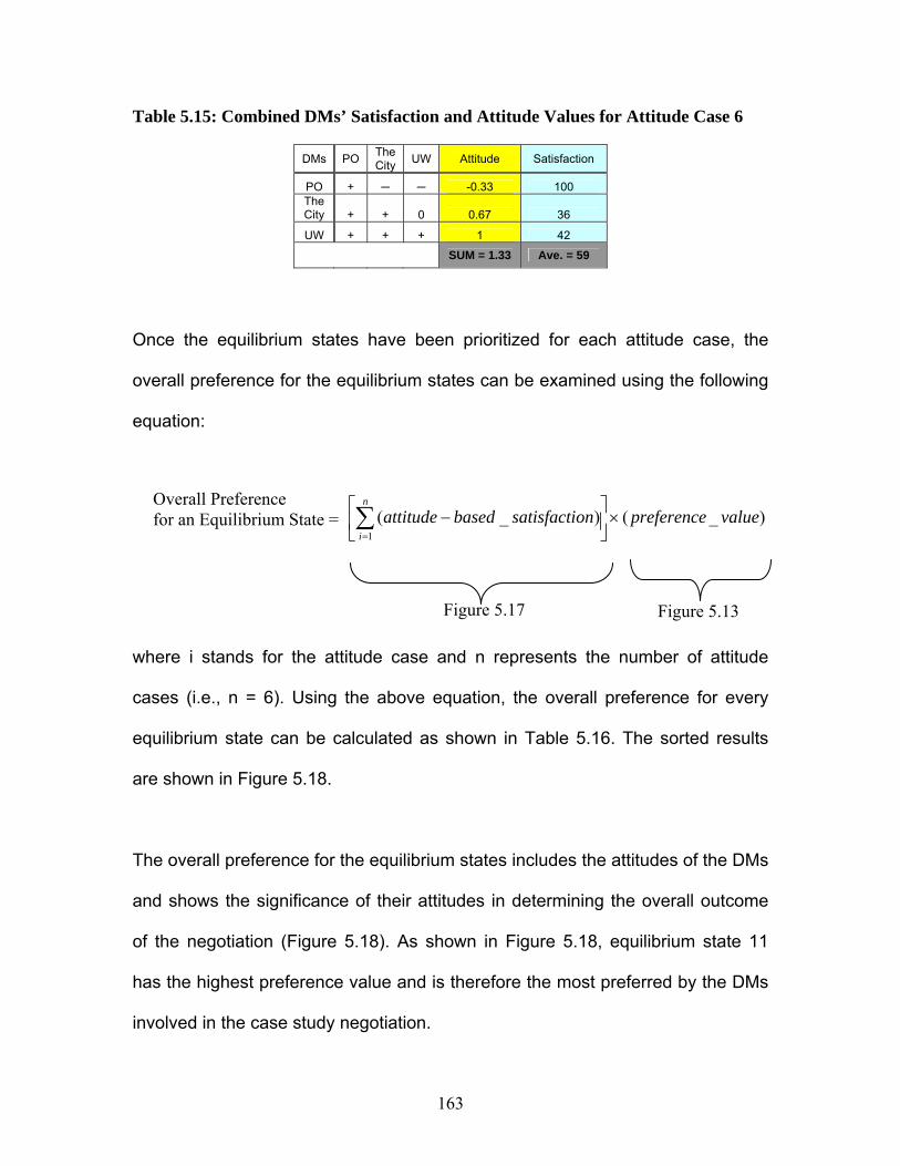
163
Table 5.15: Combined DMs’ Satisfaction and Attitude Values for Attitude Case 6
Once the equilibrium states have been prioritized for each attitude case, the
overall preference for the equilibrium states can be examined using the following
equation:
)_()_(1
valuepreferenceonsatisfactibasedattituden
i×⎥
⎦
⎤⎢⎣
⎡−∑
=
where i stands for the attitude case and n represents the number of attitude
cases (i.e., n = 6). Using the above equation, the overall preference for every
equilibrium state can be calculated as shown in Table 5.16. The sorted results
are shown in Figure 5.18.
The overall preference for the equilibrium states includes the attitudes of the DMs
and shows the significance of their attitudes in determining the overall outcome
of the negotiation (Figure 5.18). As shown in Figure 5.18, equilibrium state 11
has the highest preference value and is therefore the most preferred by the DMs
involved in the case study negotiation.
DMs PO The City UW Attitude Satisfaction
PO + ─ ─ -0.33 100 The City + + 0 0.67 36
UW + + + 1 42
SUM = 1.33 Ave. = 59
Overall Preference for an Equilibrium State =
Figure 5.17 Figure 5.13

164
Table 5.16: Overall Preference for the Equilibrium States
EquilibriumState Calculations Result
0 (28 + 56) × 36 3,024 1 (28) × 36 1,008 2 (59 + 78) × 59 8,083 3 (28) × 32 896 4 (28 + 56) × 28 2,352 6 (28) × 18 504 7 (28 + 63) × 20 1,820 8 (78) × 90 7,020 9 (63 + 78) × 83 11,703 10 (56 + 72) × 81 10,368 11 (56 + 63 + 72) × 75 14,325 14 (56 + 63) × 61 7,259 17 (63) × 69 4,374
Equilibrium States
0
2000
4000
6000
8000
10000
12000
14000
16000
11 9 10 2 14 8 17 0 4 7 1 3 6
Overall Peference
Figure 5.18: Overall Preference Sorted for the Resulting Equilibrium States
165
State 11 represents a situation in which PO cleans up the site quickly, the City
neither provides incentives nor takes legal action, and UW does not construct a
school of pharmacy. On the other hand, equilibrium state 6 has the lowest
preference value and is therefore least preferred by the DMs. Equilibrium state 6
represents a situation in which PO cleans up the site slowly, the City both
provides incentives and takes legal action, and UW does not construct a school
of pharmacy in the decontaminated site.
5.7.3.1. Updated level of information for the case study
As mentioned in Section 5.3, this real-life brownfield negotiation was modeled
and analyzed based on the amount of information available in 1997 at the
beginning of the multiple-DM negotiations among PO, the City and UW.
Therefore, the overall results obtained and shown in Figure 5.18 are based on
the amount of information available at that time and are also based on the
attitudes of the DMs during the negotiations that took place in 1997. Because this
particular real-life brownfield negotiation was very lengthy, and many rounds of
negotiation took place, a number of new circumstances arose and a great deal of
the information (e.g., the attitudes of the DMs toward one another) was updated.
Based on this updated information, the brownfield negotiation was therefore
remodeled and reanalyzed using the proposed negotiation methodology.
The overall results show that equilibrium state 8 has the highest preference
among the DMs involved and therefore, equilibrium state 8 was selected as the

166
final most beneficial decision option at the strategic level for the real-life
brownfield negotiation. Equilibrium State 8 represents a situation in which PO
cleans up the land quickly, the City does not take legal action and provides
incentives for PO and UW, and UW constructs a school of pharmacy on the
decontaminated site. This strategic outcome was further negotiated in detail by
the DMs at the tactical level. The proposed negotiation methodology at the
tactical level involving multiple DMs is discussed in Chapter 7.
5.8. Evolution of the Brownfield Conflict
The best overall strategic decision, obtained in the previous sections was found
using the proposed strategic negotiation methodology. The objective of this
section is to present discussions about how this real-life conflict was actually
resolved over time. To achieve this objective, a state transition chart is used as
shown in Table 5.17. To interpret this table, the states are considered from left to
right for which an arrow indicates an option change between two adjacent states.
Table 5.17: State Transitions for the Brownfield Conflict
Status Quo State Final StateDM Options 1 3 14 10 8
1) Slow Y Y N N N PolyOne
2) Fast N N N Y Y
3) Incentives N Y Y Y Y City
4) Legal Action N N N N N
UW 5) Construction N N N N Y

167
As shown in Table 5.17, state 1 represents the status quo of the conflict or the
initial situation of the conflict among PolyOne, the city, and UW. It should be
noted that state 1 was also one of the equilibrium states when attitude case 4 is
assumed (Figure 5.10). Attitude case 4 represents a situation in which the DMs
have negative attitudes towards one another. After initial rounds of negotiations,
the city decided to provide incentives for the other DMs and, thus, the conflict
moved from state 1 to state 3. As shown in Figure 5.10, although state 3 is an
equilibrium under attitude case 4, there was less degree of hostility among the
DMs at this stage of the conflict. Due to further rounds of negotiations, PolyOne
decided to stop slow remediation and, hence, the conflict moved to state 14,
which is also one of the equilibrium states for attitude case 2, which represents a
situation in which the DMs do not have negative attitudes towards one another
anymore.
The cooperative negotiations among the DMs continued until PolyOne decided to
remediate the site quickly and, therefore, the conflict moved to state 10 (Table
5.17) which is one of the equilibrium states for attitude cases 1 and 2. In the final
stage of cooperative negotiations, UW decided to construct a school of pharmacy
at the decontaminated site and eventually the conflict moved to state 8 or the
final stage of the conflict, as shown in Table 5.17. State 8 represents the situation
that actually occurred with respect to this case study. Therefore, the following two
insights can be concluded:
168
1. The conflict resolution proposed by the negotiation methodology,
developed in this chapter, is consistent with the real resolution for this
real-life conflict; and
2. As shown in Figure 5.10, state 8 is an equilibrium state for only attitude
case 5 which represents a situation when all of the DMs have positive
attitudes towards one another. In other words, when the DMs decide to
have positive attitudes towards one another, a more beneficial and
preferable outcome (i.e., state 8) is reached.
The results of coalition analysis of this real-life case study show that PolyOne
and UW have a possible joint move from state 14 to state 8 (Table 5.17). In other
words, PolyOne could accept to remediate the brownfield site quickly and at the
same time, UW could accept to build a school of pharmacy at the
decontaminated site. If such possible move could happen, state 10, which was
an equilibrium state, would be unstable because of an equilibrium jump and
could not be considered as an equilibrium state when coalition analysis is carried
out. More discussion about coalition analysis is provided by Kilgour et al. (2001),
Inohara and Hipel, (2008a), and Inohara and Hipel, (2008b).
5.9. Summary
This chapter has presented an attitude-based strategic negotiation methodology
that was developed with multiple DMs. The Graph Model for Conflict Resolution
(GMCR) was systematically employed in order to study the negotiations at two
169
stages: modeling and analysis. In the modeling stage, the DMs and their options
were determined, infeasible states were removed, and the DMs’ state rankings
were determined. In the analysis stage, stability analysis that considered the
attitudes of the DMs was conducted. Algorithms were proposed for removing
infeasible attitude cases in negotiations involving multiple DMs. From the
resulting feasible attitude cases, six relevant cases were selected, and attitude-
based stability analysis was performed.
To discuss the results of the stability analysis, two approaches were applied:
qualitative and quantitative. In the qualitative approach, which is the regular
method used in GMCR, the resulting equilibrium states were examined and the
preference for the states was investigated. To support the qualitative approach, a
quantitative approach or an ad hoc analysis has been performed for discussing
and examining the resulting equilibrium states in order to determine a
quantitative relationship between the DMs’ attitudes and the DMs’ satisfaction
values. The quantitative approach supports the qualitative approach in
determining which equilibrium state is most preferred in overall by the DMs when
the influence of the attitudes of the DMs on the outcome of the negotiation is
taken into account.
The results of the analyses were used to determine the most beneficial outcome
of the negotiations at the strategic level. The findings of the discussion were
summarized in a proposed equation for obtaining the overall preference for every
170
equilibrium state. Based on the updated amount of information for this real-life
brownfield negotiation, the final result indicates that equilibrium state 8 is the
most preferred and beneficial decision option at the strategic level. To examine
the proposed resolution, a state transition table was developed and the real-life
conflict evolution was discussed. The results of the discussions indicate that
state 8 represents the situation in which this real-life case study was actually
resolved over time and, thus, the proposed resolution can be confirmed.
Therefore, equilibrium state 8 will be further negotiated at the tactical level as
proposed in Chapter 7.
This research provides valuable insight into the influence of the attitudes of the
DMs on the outcome of strategic negotiations. The importance of the research in
this chapter lies in proposal of a negotiation methodology that helps DMs
determine which attitudes are needed in order to guide negotiations to more
preferable decisions and prevent attitudes that can result in unwanted
consequences for all participants concerned.
171
CHAPTER 6: Attitude-Based Tactical Negotiation Involving Two Decision Makers
6.1. Introduction
This chapter presents the tactical level of the attitude-based negotiation
methodology for resolving construction conflicts when two decision makers are
involved. To demonstrate the benefits of the proposed methodology, the
brownfield negotiation case study, introduced in Chapter 4, is used to develop
the methodology. The tactical level of the negotiation methodology complements
the strategic level developed in Chapter 4 and therefore, this chapter supports
and complements Chapter 4 where a brownfield conflict case study with two
Decision Makers (DMs) was used to model the strategic level of the negotiation
methodology. The DMs considered their attitudes toward each other and
interactively negotiated in order to reach strategies that would improve their own
positions in their pair-wise negotiation. Using GMCR approach, three negotiation
situations, corresponding to the three types of DMs’ attitudes toward each other,
were modeled. Three sets of possible outcomes, expressed as strategic solution
options for the conflict, were then obtained and evaluated by the DMs in order to
find the most beneficial decision. Consequently, the DMs chose equilibrium state
2 as the strategic decision.
172
Although it is crucial for the DMs to agree on a strategic decision, it is not the
final and sustainable solution for the conflict. The strategic decision identifies only
a DM’s best course of action and advises the DM which actions are in a
particular DM’s interest and which responses would be in the interests of the
other DM. The strategic decision does not provide further detailed information
(e.g., the specific amount of the redevelopment costs) about the resulting
strategic decision for which a detailed mutual agreement can be reached.
Therefore, a tactical negotiation approach is needed with the goal of specifying
the specific amount of compromise that each DM should make with respect to
each conflicting issue. The primary objective of Chapter 6 is to propose such
complementary tactical negotiation approach when only two DMs are involved in
the tactical negotiation.
6.2. Tactical Negotiation Methodology: A Brownfield Case Study
The brownfield negotiation case study presented in Chapter 4 is further
developed in this section to model the tactical negotiation methodology. It is
assumed that the negotiations between the DMs (i.e., the owner and the
government) in the case study, take place before the start of the brownfield
redevelopment. It is also assumed that both DMs have agreed on outcome 2 as
the most beneficial strategic outcome obtained from the strategic analysis using
GMCR. The development of tactical negotiation consists of some steps
demonstrated in the following subsections.

173
6.2.1. Step 1: Identify Conflicting Issues within the Strategic Decision
The outcomes chosen at the strategic level as possible solutions for the conflict
include one or more negotiating issues that can be further negotiated at a more
detailed level. The negotiation issues can be continuous (numeric or accurate; as
it is in this case study), discrete (nonnumeric or linguistic) or the combination of
both continuous and discrete issues. Because the owner and the government
have strategically decided to consider outcome 2 as the possible solution, they
need to explicitly identify and define the conflicting issues involved in outcome 2
and develop a scale for each issue to represent potential points of compromise
between their initial negotiation positions. Outcome 2 represents a scenario in
which the owner does not accept liability and sells the property, and the
government neither shares the costs nor takes the case to court. Hence, the
selling price of the owner’s property is the only numeric negotiation issue
involved in outcome 2. It is reasonable to presume that the owner expects to sell
her property at the highest price and that the government prefers to buy it at the
lowest price. The goal of the proposed negotiation approach is to provide the
owner and the government with the amount of compromise needed to reach a
reasonable mutual agreement about the selling price. To achieve this goal, the
concept of utility function is employed and explained as follows,
6.2.2. Step 2: Determine the DMs’ Utility Functions
Utility analysis deals generally with relative satisfaction from the results of
decision making. A utility is a function of an action and the state of the
174
environment (i.e., U (A, E)). If a DM has to rank the consequences in order of his
preferences, it is convenient to represent preferences with a utility function and
reason indirectly about the preferences by means of these utility functions. Utility
function forms represent and describe, for each DM, the tradeoffs between
consequences (Keeney and Raiffa, 1976). If an appropriate utility is assigned to
each possible consequence and the expected utility of each alternative is
calculated, then the best course of action is the alternative with the highest
expected utility (Du and Chen, 2007). In other words, when cardinal utility
analysis is used, DMs try to maximize their own expected utility, and if they
cooperatively negotiate, they strive to maximize their joint expected utility value.
More discussions about utility theory are provided by Keeney and Raiffa (1976)
and Kilgour (2006).
The key characteristic of utility functions is that they are often monotonic, which
means that they are constantly increasing and never decreasing or constantly
decreasing and never increasing in value (Keeney and Raiffa, 1976). For
example, when a monetary asset position is appropriate for summarizing
consequences, most DMs prefer a greater amount to a lesser amount, and the
utility function increases monotonically. When the preferences for response time
to calls for emergency services are considered, a smaller response time is
always preferred to a larger one. Such a utility function is monotonically
decreasing.

175
The expected utility theory was originally developed by Von Neumann and
Morgenstern (1944). The theory states that a DM chooses between risky or
uncertain prospects by comparing their expected utility values (i.e., the weighted
sums obtained by adding the utility values of outcomes multiplied by their
respective probabilities). A critical step in many applications of decision analysis
under the utility hypothesis is the specification and estimation of a suitable utility
function form. For this purpose, several studies have been carried out such as
those by Du and Chen (2007), Halter and Dean (1971), Cheung and Suen
(2002), Musser et al. (1984), Keeney and Raiffa (1976), Pena-Mora and Wang
(1998), Mumpower (1988), Darling and Mumpower (1991), Zuhair et al. (1992),
Lin et al. (1974), Kersten (2001), Ji et al. (2007), Zhang et al. (2005), Lin and
Chang (1978), and Zeleznikow et al. (2007). The form of a utility function
depends on the characteristics of the DMs who have a specific attitude with
respect to their risk and preferences for consequences. These attitudes can be
mathematically expressed in terms of some of the properties of the DMs’ utility
functions. For example, a DM’s utility function can be considered to be an
exponential function such as f(x) = -e-bx. If parameter “b” represents the attitude
of the DM, then changes in the value of “b” cause changes in the exponential
function form, so the expected utility value for the DM changes. If a DM
subscribes to a specific attitude, his utility function is restricted to a degree, and
hence, the real assessment of his utility function is simplified.

176
Of the utility functional forms suggested in the literature, the polynomial and
exponential functions seem to be the most popular (Zuhair et al., 1992). Buccola
(1982) reported that polynomial and exponential functions give the same optimal
portfolio. Keeney and Raiffa (1976) extensively studied the form and properties of
some utility functions. Kirkwood (1997) believed that exponential utility functions
are convenient to work with but they may not reflect all DMs’ preferences.
Additionally, some researchers, such as Howard (1971) and Savage (1971),
considered exponential utility functions as reasonable approximations of the
preferences of the DMs. On the other hand, Eliashberg and Winkler (1978)
studied the linear and nonlinear forms of utility functions. They reported that
some nonlinear graphs, such as polynomial function forms, may provide a better
understanding of the effect of utility functions on the solutions to the conflict. In
contrast to the exponential utility function, which imposes only risk aversion on all
DMs, the polynomial utility functions are more flexible for assigning risk attitudes
(either risk aversion or risk preference) to DMs (Zuhair et al., 1992; Pena-Mora
and Wang, 1998). Accordingly, the utility function forms proposed for the DMs
involved in this case study are derived from Polynomial functions defined in the
following:
Polynomial function: f(x) = anxn + an-1xn-1 + ... + a1x + a0 [1]
Where f(x) is the utility function, “x” is an input variable, “a” is a real number
coefficient, and “n” is the power of function. The value of “n” must be a
nonnegative value and the degree of the polynomial function is the highest value
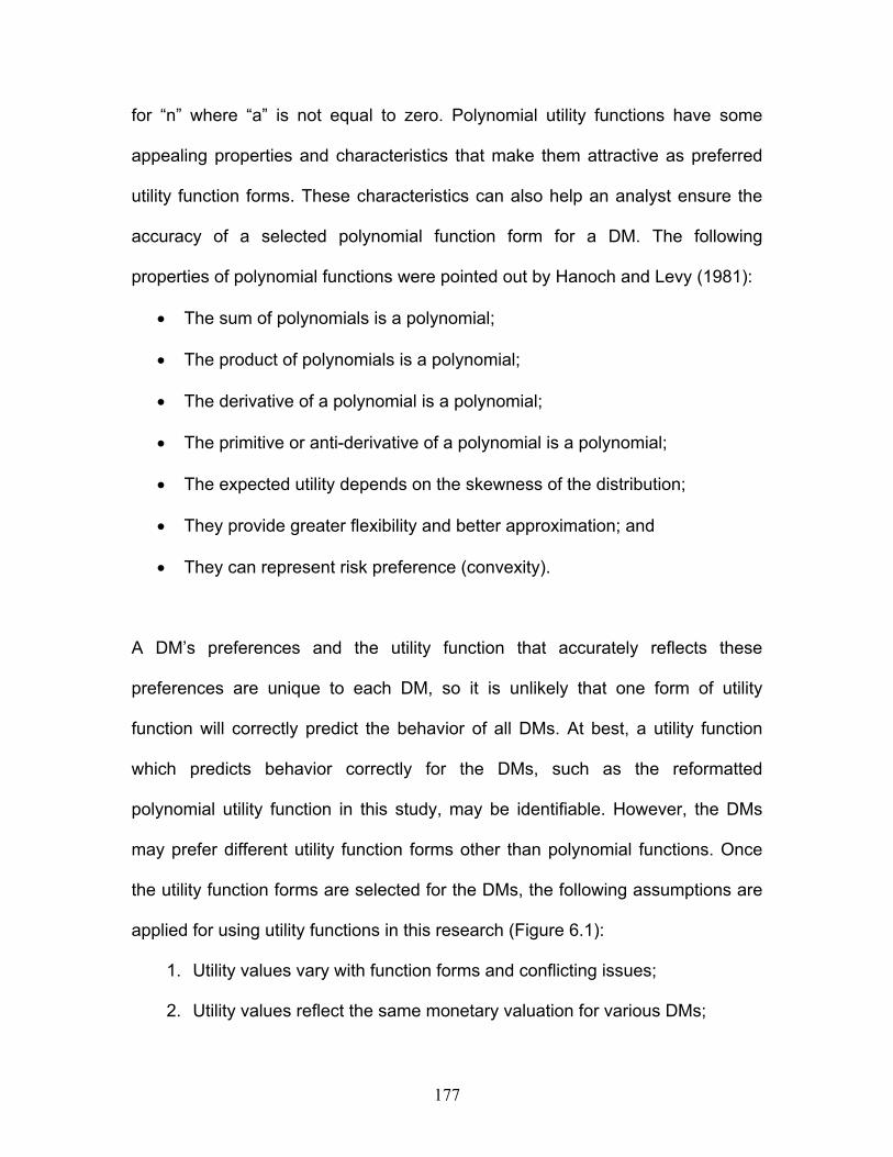
177
for “n” where “a” is not equal to zero. Polynomial utility functions have some
appealing properties and characteristics that make them attractive as preferred
utility function forms. These characteristics can also help an analyst ensure the
accuracy of a selected polynomial function form for a DM. The following
properties of polynomial functions were pointed out by Hanoch and Levy (1981):
• The sum of polynomials is a polynomial;
• The product of polynomials is a polynomial;
• The derivative of a polynomial is a polynomial;
• The primitive or anti-derivative of a polynomial is a polynomial;
• The expected utility depends on the skewness of the distribution;
• They provide greater flexibility and better approximation; and
• They can represent risk preference (convexity).
A DM’s preferences and the utility function that accurately reflects these
preferences are unique to each DM, so it is unlikely that one form of utility
function will correctly predict the behavior of all DMs. At best, a utility function
which predicts behavior correctly for the DMs, such as the reformatted
polynomial utility function in this study, may be identifiable. However, the DMs
may prefer different utility function forms other than polynomial functions. Once
the utility function forms are selected for the DMs, the following assumptions are
applied for using utility functions in this research (Figure 6.1):
1. Utility values vary with function forms and conflicting issues;
2. Utility values reflect the same monetary valuation for various DMs;
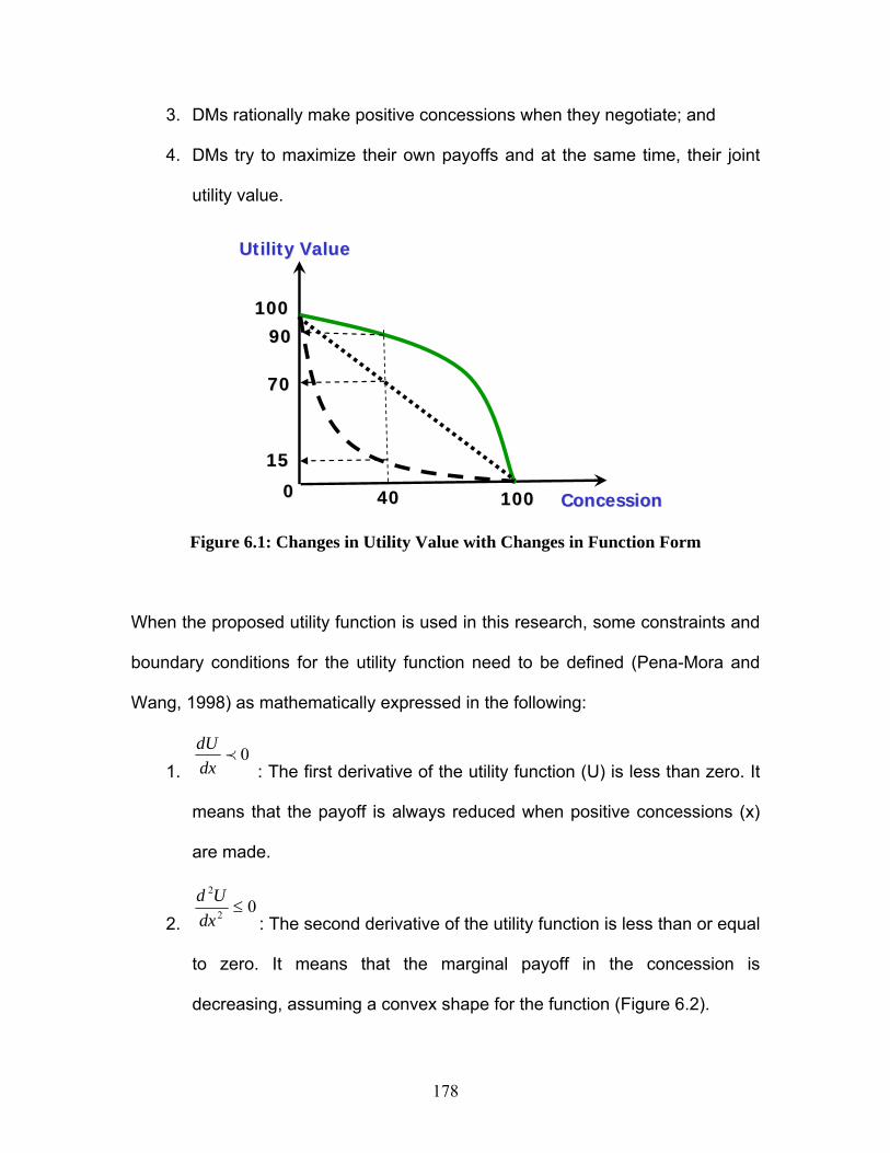
178
3. DMs rationally make positive concessions when they negotiate; and
4. DMs try to maximize their own payoffs and at the same time, their joint
utility value.
ConcessionConcession
Utility ValueUtility Value
1515
9090
7070
404000 100100
100100
Figure 6.1: Changes in Utility Value with Changes in Function Form
When the proposed utility function is used in this research, some constraints and
boundary conditions for the utility function need to be defined (Pena-Mora and
Wang, 1998) as mathematically expressed in the following:
1. 0p
dxdU
: The first derivative of the utility function (U) is less than zero. It
means that the payoff is always reduced when positive concessions (x)
are made.
2. 02
2
≤dx
Ud: The second derivative of the utility function is less than or equal
to zero. It means that the marginal payoff in the concession is
decreasing, assuming a convex shape for the function (Figure 6.2).

179
3. 1000 ≤≤ x : The concession value is normalized between zero and 100.
4. 1000 ≤≤U : The maximum and minimum values for the expected utility
are 100 and zero, respectively. It means that if 100% of the payoff has to
be made, no compromise should be made (x = 0); that is, U(0) = 100.
The payoff is minimized to zero if a complete concession is made; that is,
U(100) = 0.
It can be noted that the above assumptions, constraints, and boundary conditions
can also assist DMs in selecting an appropriate utility function form which is
calibrated based on the DMs’ attitudes preferences. Moreover, an analyst (e.g., a
mediator) can provide a questionnaire for each DM who can describe their
behavior with respect to the other DMs involved in a dispute. The analyst can
then collect the questionnaires and select an appropriate form of utility function
for every DM involved.
According to the above discussion and with respect to the brownfield negotiation
case study, the DMs start their tactical negotiation by selecting a proper utility
function. The general form of utility function for the seller (owner) and the buyer
(government) is shown in Figure 6.2a. These shapes reflect the seller’s highest
preference to get the highest price and, at the same time, the buyer’s highest
preference to pay the lowest price. Generalizing these functions, various
polynomial forms can be generated for the owner and the government, as shown
in Figures 6.2b and 6.2c, respectively. Because the government’s position on the

180
Util
ity
Seller’s Utility (high price is preferred)
Buyer’s Utility (low price is preferred)
H L
1 Price ($m) 10
0
1
(a)
))(100( 1)(
nnowner xU −= nn
government xU )100)(100( 1)( −= −
(b) (c)
Seller (owner) Buyer (government)
Figure 6.2: The DMs’ Utility Functions for the “Price” Issue
n=0.1
n=0.4n=0.7
n=1n=3
n=5n=7
n=10
0
10
2030
40
5060
70
8090
100
0 10 20 30 40 50 60 70 80 90 100Price (%)
Utility (%)
n=0.1
n=0.4
n=0.7
n=1
n=3
n=10
0
10
20
30
40
50
60
70
80
90
100
0 10 20 30 40 50 60 70 80 90 100
price (%)
Utility (%)
price of the property is in contrast to the owner’s position, the government’s utility
function is a mirror image of the owner’s function ( Du and Chen, 2007; Pena-
Mora and Wang, 1998).
6.2.3. Step 3: Obtain an Integrated Utility Function for Each Issue
Once an appropriate utility function was selected for the owner and the
government, the interactive negotiation process between the DMs is modeled. An
approach to the modeling is presented below. In this approach, the utility
functions of the DMs are integrated to one coordinated system, as shown in
Figure 6.3.
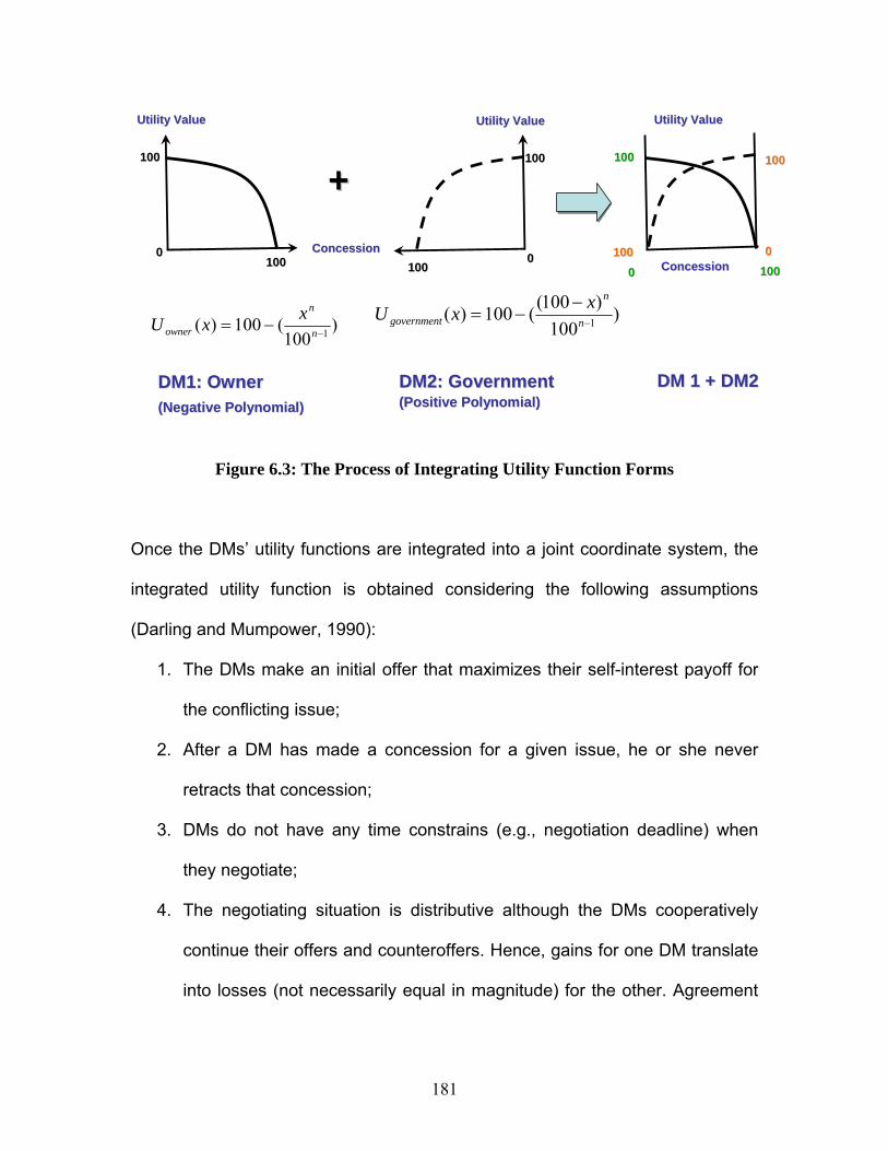
181
DM1: OwnerDM1: Owner(Negative Polynomial)(Negative Polynomial)
ConcessionConcession
Utility ValueUtility Value
00100100
Utility ValueUtility Value
100100
100100
00 ConcessionConcession
Utility ValueUtility Value
100100100100
100100
++100100
DM2: GovernmentDM2: Government(Positive Polynomial)(Positive Polynomial)
DM 1 + DM2DM 1 + DM2
0000
)
100(100)( 1−−= n
n
ownerxxU
)
100)100((100)( 1−
−−= n
n
governmentxxU
100100
Figure 6.3: The Process of Integrating Utility Function Forms
Once the DMs’ utility functions are integrated into a joint coordinate system, the
integrated utility function is obtained considering the following assumptions
(Darling and Mumpower, 1990):
1. The DMs make an initial offer that maximizes their self-interest payoff for
the conflicting issue;
2. After a DM has made a concession for a given issue, he or she never
retracts that concession;
3. DMs do not have any time constrains (e.g., negotiation deadline) when
they negotiate;
4. The negotiating situation is distributive although the DMs cooperatively
continue their offers and counteroffers. Hence, gains for one DM translate
into losses (not necessarily equal in magnitude) for the other. Agreement
182
is needed, and neither DM can abdicate or withdraw from the dispute prior
to reaching an agreement;
5. The DMs engage in a negotiation in which each alternately makes a new
offer that changes by the same amount each time. Each DM can make
only a 10-unit concession on a scale of 0 – 100, and neither can bypass
the concession process; and
6. When the integrated utility function reaches the maximum point, the DMs
jointly gain the maximum payoff (i.e., satisfaction). The maximum point is
used to determine the DMs’ concession. No further concessions by either
DM with respect to that issue can be made, and the tactical negotiation is
concluded.
The above assumptions are used to conduct a pair-wise tactical negotiation
using the DMs’ utility functions to obtain an integrated utility function. According
to the above assumptions, an integrated utility function is used to obtain the
exact amount of the concession each DM should make with respect to conflicting
issues (Ji, et al. 2007; Mumpower, 1991; Pena-Mora and Wang, 1998).
To generalize and clarify the integrating process, it is assumed that the owner
represents DM 1 and the government represents DM 2 as shown in Figure 6.4.
Both DMs intend to cooperatively negotiate to obtain the optimum resolution for
the conflicting issue (i.e., the owner’s selling price). In other words, they want to
cooperatively negotiate and sequentially reach to a point in which their joint
satisfaction is maximized.
183
The negotiation process opens with DM 1 proposing an offer that initially
maximizes her individual utility function with a zero concession level, indicated as
point A in Figure 6.4. Point A stands for 100% integrated gain for both DMs in
which UDM1(0) = 100% gain for DM 1 and UDM2(100) = 0% gain for DM 2.
Similarly, DM 2 makes an initial counteroffer to maximize his payoff with zero
concession as shown with point C in Figure 6.4. Point C also stands for 100%
integrated gain for both DMs in which UDM2(0) = 100% gain for DM 2 and
UDM1(100) = 0% gain for DM 1. Points A and C thus constitute the first and last
points of the integrated utility function. Because the negotiation process is
cooperative and both DMs want to reach an agreement, each time DM 1
proposes a 10% concession, DM 2 also makes a counteroffer with a 10%
Concession (%)
Utility (%)
100 100
Maximum Utility
Integrated Utility Function
A
B
C
Figure 6.4: Tactical Negotiation Process Involving Two DMs
DM 1 DM 2
D
E
F
G
H
I
J
K
L
M
N0 10 20 30 40 50 60 70 80 90 100%
100 90 80 70 60 50 40 30 20 10 0%P
184
concession. Each concession made by each DM corresponds to one point on the
integrated utility function. Continuing this process, the integrated utility function
shape is sequentially drawn from both sides.
Point H, for example, on the integrated utility function, shown in Figure 6.4, is
considered. Line DF in Figure 6.4 represents the marginal payoff gain for DM 1
when a 30% concession is made by DM 1, whereas line DE represents the
marginal payoff gain for DM 2 when a 70% concession is made by DM 2. To
obtain the position of point H (i.e., the DMs’ joint gain or satisfaction), the gains
by the DMs are algebraically summed to calculate the height of DH = DE + DF.
The same procedure is carried out to obtain point M (Figure 6.4). In this case, I J
represents the payoff gain by DM 1 when a 70% concession is made by DM 1
and I K represents gain for DM 2 when a 30% concession is made by DM 2. The
position of M is obtained by summing up the gains by the DMs. That is, I M = I J
+ I K.
Following this procedure, the DMs continue to compromise sequentially until the
maximum point on the total utility function (B) is eventually reached. The
maximum point represents the settlement point or the point of agreement
because both DMs receive the highest joint payoff. This means that both DMs
have reached the highest degree of satisfaction for their cooperative effort. The
settlement point is used to obtain the concession indicated on the horizontal axis.
In Figure 6.4, point N indicates the concession (40%) that DM 1 should make and
185
point P indicates the concession (60%) that DM 2 should make to reach a mutual
agreement regarding the selling price of the owner’s property. The settlement
point can also be mathematically obtained by optimizing the following equation:
)()()(
1iji
k
jjiii xUWxU ×= ∑
=
−
[2]
Where )( ii xU−
is the integrated utility function for issue i, Wji is the weight for issue
i of DM j, Uji is the utility function for issue i of DM j, and xi is the concession
variable for issue i.
6.2.4. Step 4: Select the Best Decision Value
Figure 6.5 represents a situation in which the owner prefers to have a
cooperative attitude and a desire to sell the property and avoid all risks involved
with the brownfield property. Therefore, a utility function with n = 7 is a good
representation of the owner who is willing to compromise more than the
government. On the other hand, the government prefers to be cooperative but
has no great interest in buying the contaminated property. As such, a utility
function form with n = 2 is a good representation of the government who is willing
to concede less than the owner.
The integrated utility function obtained graphically in Figure 6.5, can be
mathematically expressed as follows:
[3] )()(int ggooegrated UwUwU ×+×=
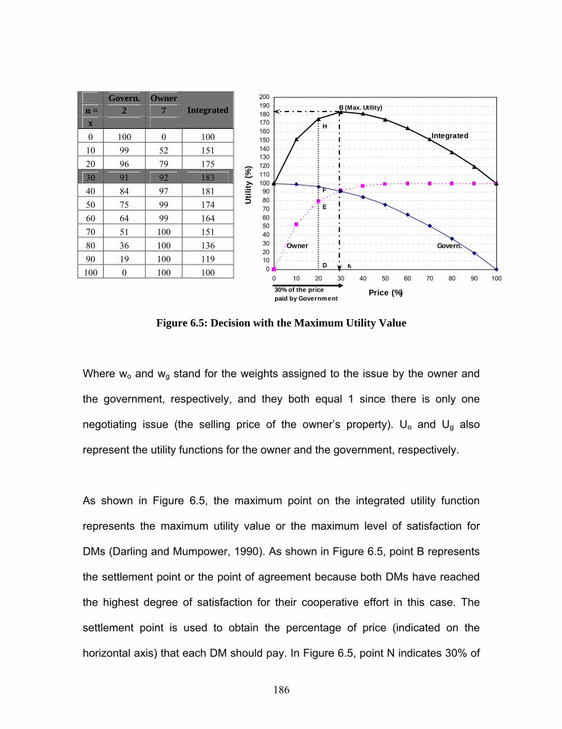
186
Owner Govern.
Integrated
0102030405060708090
100110120130140150160170180190200
0 10 20 30 40 50 60 70 80 90 100
Price (%)
Util
ity (%
)
E
D
F
H
N
B (Max. Utility)
30% of the pricepaid by Government
Figure 6.5: Decision with the Maximum Utility Value
Where wo and wg stand for the weights assigned to the issue by the owner and
the government, respectively, and they both equal 1 since there is only one
negotiating issue (the selling price of the owner’s property). Uo and Ug also
represent the utility functions for the owner and the government, respectively.
As shown in Figure 6.5, the maximum point on the integrated utility function
represents the maximum utility value or the maximum level of satisfaction for
DMs (Darling and Mumpower, 1990). As shown in Figure 6.5, point B represents
the settlement point or the point of agreement because both DMs have reached
the highest degree of satisfaction for their cooperative effort in this case. The
settlement point is used to obtain the percentage of price (indicated on the
horizontal axis) that each DM should pay. In Figure 6.5, point N indicates 30% of
Govern. Owner n = 2 7
x Integrated
0 100 0 100 10 99 52 151 20 96 79 175 30 91 92 183 40 84 97 181 50 75 99 174 60 64 99 164 70 51 100 151 80 36 100 136 90 19 100 119 100 0 100 100

187
the price is paid by the government and 70% (100%-30%) of the price is
conceded by the owner. If the initial price of the property is $200,000, for
example, the government should pay $60,000 (0.3 × $200,000) and the owner
should concede $140,000 (0.7 × $200,000).
As it can be seen, the proposed tactical negotiation methodology assists the DMs
to determine the specific concession needed to reach a mutual tactical
resolution. It should be mentioned that disagreement point “d” (Kilgour, 2006)
was not considered in this case study. The disagreement point represents the
DMs’ minimum utility values that the DMs can count on it if they do not reach any
agreement. The individual rationality condition is that no DM receives less utility
than he or she would receive at “d”. Of course, it is guaranteed that the DMs can
achieve “d”. The disagreement point will be considered in the tactical negotiation
methodology involving multiple DMs proposed in Chapter 7. Moreover, in this
case study only one conflicting issue (i.e., the selling price of the owner’s
property) was considered. Considering multiple conflicting issues will be also
discussed in Chapter 7.
6.3. Sensitivity to the DMs’ Attitudes
A major contribution of this chapter is related to the incorporation of the DMs’
attitudes into the proposed negotiation methodology. As the influence of DMs’
attitudes on strategic negotiations was investigated in Chapters 4 and 5, it is
important to assess the effect of DMs’ attitudes on tactical negotiation outcomes.

188
In the proposed negotiation methodology, the attitudes of the DMs can be
reflected by the power of the reformatted polynomial utility function (n):
As shown in Figure 6.2, the shape of utility function changes with the value of “n”.
When 0 < n < 1, then the polynomial function has a negative convex shape for
the government and positive convex shape for the owner. When 1 < n ≤ 10, then
the utility function has a negative concave shape for the government and positive
concave shape for the owner. The function shape is linear when n = 1. (Ji et al.
2007). It can be noticed that each value of “n” reflects the specific attitude of a
DM. Moreover, the function forms when 1 < n ≤ 10 reflect decreasing marginal
improvements in the utility as the values of the concessions approach the DM’s
ideal. Thus, the shape of the integrated utility function form depends on the
power of the DMs’ utility functions. When the shape of integrated utility function
changes, the position of the maximum point on the integrated function also
changes, and this change in maximum point indicates a different settlement point
and thereby, different concession values for each DM. In other words, the
change in the position of maximum point on the integrated utility function
indicates that the maximum level of satisfaction for both DMs has changed.
Figure 6.6 displays four scenarios in the tactical negotiation case study in which
the owner and the government express different attitudes toward each other (i.e.,
different function forms corresponding to different attitudes were selected). These
attitude scenarios are analyzed below. It should be noted that several other
)100
(100)( 1−−= n
nxxU
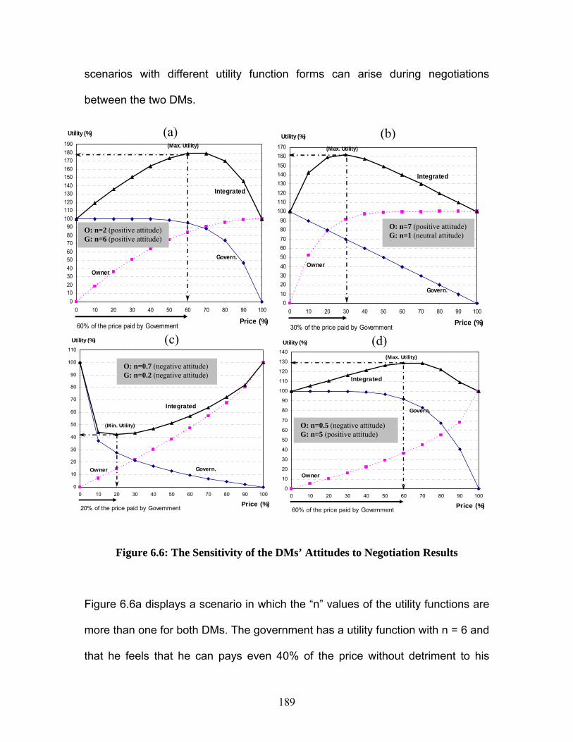
189
Owner
Govern.
Integrated
0102030405060708090
100110120130140150160170180190
0 10 20 30 40 50 60 70 80 90 100
Price (%)
Utility (%)
(Max. Utility)
60% of the price paid by Government
O: n=2 (positive attitude) G: n=6 (positive attitude)
Owner
Govern.
Integrated
0102030405060708090
100110120130140150160170
0 10 20 30 40 50 60 70 80 90 100
Price (%)
Utility (%)
(Max. Utility)
30% of the price paid by Government
O: n=7 (positive attitude) G: n=1 (neutral attitude)
Owner Govern.
Integrated
0
10
20
30
40
50
60
70
80
90
100
110
0 10 20 30 40 50 60 70 80 90 100
Price (%)
Utility (%)
(Min. Utility)
20% of the price paid by Government
O: n=0.7 (negative attitude) G: n=0.2 (negative attitude)
Owner
Govern.
Integrated
0
10
20
30
40
50
60
70
80
90
100
110
120
130
140
0 10 20 30 40 50 60 70 80 90 100
Price (%)
Utility (%)
(Max. Utility)
60% of the price paid by Government
O: n=0.5 (negative attitude) G: n=5 (positive attitude)
(a) (b)
(c) (d)
scenarios with different utility function forms can arise during negotiations
between the two DMs.
Figure 6.6: The Sensitivity of the DMs’ Attitudes to Negotiation Results
Figure 6.6a displays a scenario in which the “n” values of the utility functions are
more than one for both DMs. The government has a utility function with n = 6 and
that he feels that he can pays even 40% of the price without detriment to his
190
position because if he pays 40% of the price, he can still receive a 100% payoff.
On the other hand, the owner has a utility function with the power value of n = 2.
Considering the owner’s graph, it can be seen that the owner is able to reduce
only 10% of the initial price of its property without detriment to her position
because if she makes up to a 10% concession to sell its property, she can still
receive a 100% payoff. The individual payoff values for both DMs thus start to
decrease after 40% and 10% concessions made by the government and the
owner, respectively. It can be concluded for this case that the government, with a
higher “n” value, is more cooperative than the owner, who has a lower “n” value.
The “integrated” graphs in Figure 6.6 have been drawn using the procedure
illustrated in Figure 6.4. It can also be seen that the maximum point on the
integrated graph represents the settlement point of the negotiation which is 179%
for this scenario shown in Figure 6.6.a. This settlement point indicates on the
horizontal axis that the government pays for the 60% of the price and the owner
reduces its initial offer by 40% and sells its property.
When Figure 6.6.b is considered, n(owner) = 7 is higher than n(government) = 1. It can
be seen that the owner can reduce its initial offer by 50% without detriment to its
position, whereas the government starts losing its utility when any concession is
made. It means that the government has a less cooperative attitude with respect
to the owner, who feels that the initial offer can be reduced without significantly
damaging its position. The maximum expected joint utility value for this scenario

191
is 162%, which is less than that in the previous scenario (179%). If the results of
the two scenarios are compared, the following two observations can be made:
1. Reduction of the expected joint utility value in the second scenario to
162 % comparing with the first scenario (179%) indicates that the
combination of “n” values in the first scenario (n(owner) = 2 and
n(government) = 6) is resulted in a higher expected joint utility value than
that in the second scenario (n(owner) = 7 and n(government) = 1); and
2. The location of maximum joint utility on the integrated curve is shifted
from right side of the plot in Figure 6.6a to the left side of the plot in
Figure 6.6b. In other words, in the first scenario, the government is
more cooperative (n = 6) and the owner is less cooperative (n = 2) so
that the maximum utility point is placed on the right side; whereas, in
the second scenario, the owner is more cooperative (n = 7) and the
government is less cooperative (n = 1) so that the maximum utility
point is placed on the left side.
The two bottom plots in Figure 6.6c and 6.6d depict situations for which the “n”
value for one or both DMs is less than 1 and, as can be seen, the shape of the
utility function changes from concave to convex when the “n” value is reduced
from more than 1 to less than 1. Such reduction of “n” value to less than 1 not
only can reduce the cooperative attitudes of the DMs, but can also significantly
decrease the total utility value to even less than 100%, which means that the
negotiation process is unproductive (Figure 6.6c). In other words, it would be
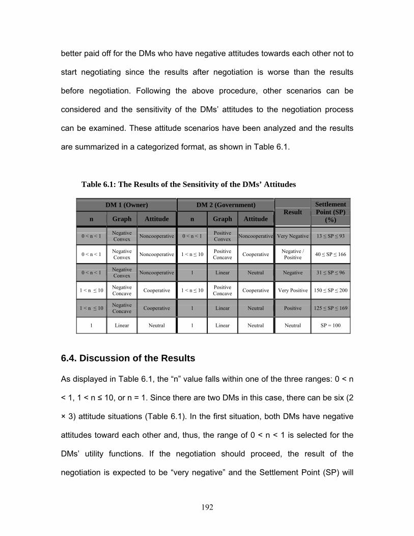
192
better paid off for the DMs who have negative attitudes towards each other not to
start negotiating since the results after negotiation is worse than the results
before negotiation. Following the above procedure, other scenarios can be
considered and the sensitivity of the DMs’ attitudes to the negotiation process
can be examined. These attitude scenarios have been analyzed and the results
are summarized in a categorized format, as shown in Table 6.1.
Table 6.1: The Results of the Sensitivity of the DMs’ Attitudes
DM 1 (Owner) DM 2 (Government)
n Graph Attitude n Graph Attitude Result
Settlement Point (SP)
(%)
0 < n < 1 Negative Convex Noncooperative 0 < n < 1 Positive
Convex Noncooperative Very Negative 13 ≤ SP ≤ 93
0 < n < 1 Negative Convex Noncooperative 1 < n ≤ 10 Positive
Concave Cooperative Negative / Positive 40 ≤ SP ≤ 166
0 < n < 1 Negative Convex Noncooperative 1 Linear Neutral Negative 31 ≤ SP ≤ 96
1 < n ≤ 10 Negative Concave Cooperative 1 < n ≤ 10 Positive
Concave Cooperative Very Positive 150 ≤ SP ≤ 200
1 < n ≤ 10 Negative Concave Cooperative 1 Linear Neutral Positive 125 ≤ SP ≤ 169
1 Linear Neutral 1 Linear Neutral Neutral SP = 100
6.4. Discussion of the Results
As displayed in Table 6.1, the “n” value falls within one of the three ranges: 0 < n
< 1, 1 < n ≤ 10, or n = 1. Since there are two DMs in this case, there can be six (2
× 3) attitude situations (Table 6.1). In the first situation, both DMs have negative
attitudes toward each other and, thus, the range of 0 < n < 1 is selected for the
DMs’ utility functions. If the negotiation should proceed, the result of the
negotiation is expected to be “very negative” and the Settlement Point (SP) will
193
be in the lowest range (13 ≤ SP ≤ 93). This means that the total (i.e., joint) utility
value reduces to even less than 100% in this case, and such a negotiation is not
productive because the joint satisfaction level for both DMs at the end of
negotiation is even lower than the individual satisfaction level for each DM at the
beginning of the negotiation. It should be remembered that the objective of the
DMs is to maximize their total utility value and when they negotiate, they try to
maximize their cooperative satisfaction.
In the second situation, DM 1 has a negative attitude (0 < n < 1) toward DM 2,
whereas DM 2 has a positive attitude (1 < n < 10) toward DM 1, and thus, 40 ≤
SP ≤ 166, and the total utility value falls within a range of positive and negative
values. Accordingly, this situation results in a better total utility value than that of
the previous situation. Following this procedure, the same discussion can be
provided for the other four attitude situations shown in Table 6.1.
It can be inferred from the six attitude situations in Table 6.1 that the higher value
for the power (n) of the utility functions is selected, the more cooperative the DMs
intend to be in their tactical negotiations. In other words, the DMs who both have
a positive attitude toward each other can expect to achieve higher satisfaction
level with higher total utility values and, as such, they may reach a “win-win”
solution with the highest satisfaction for their joint efforts. The highest total utility
value in the joint negotiation (Row 4 in Table 6.1) is called Nash equilibrium point
where both DMs have positive attitudes towards each other and have reached

194
the highest value for their joint SP. In Nash equilibrium point the DMs have no
incentive to move to other states or other attitude cases in Table 6.1.
The power of the polynomial utility function can also reflect the DMs’ risk
attitudes. In terms of the DMs’ attitudes towards risk, three types of DM are
considered: risk avoider, risk taker, and risk neutral (Keeney and Raiffa, 1976).
The results of the proposed negotiation methodology show that:
1. DMs who are more risk-averse and perhaps less cooperative prefer to
select lower values for the power (n) of their utility function;
2. DMs who are more risk-prone and perhaps more cooperative prefer to
select higher values for the power (n) of their utility function; and
3. DMs who are neutral towards risk prefer to select the power (n) of their
utility function as n = 1.
It can be seen in Table 6.1 that when 0 < n < 1, a utility function has a convex
shape and when 1 < n ≤ 10, a utility function takes a concave shape. There are
proven mathematical theorems (Kilgour, 2006; Keeney and Raiffa, 1976) that
correlate the DMs’ risk aversion level to the shape of the utility function. Risk
avers, risk prone, and risk neutral are represented by a convex, concave, or
linear function, respectively. The utility function shapes proposed in this research
are driven by those mathematical theorems. Therefore, the results of the
proposed methodology in this chapter are consistent with other research in this
area.

195
6.5. Summary
In this chapter, the development of the proposed attitude-based negotiation
methodology at the tactical level involving two decision makers was
demonstrated using the concept of utility function. The proposed methodology
supports and complements the strategic level of the negotiation methodology
developed in Chapter 4 when two decision makers were involved in the strategic
negotiation. The brownfield negotiation case study, introduced in Chapter 4, was
used in this chapter to develop the methodology. Also, the sensitivity of decision
makers’ attitudes to the outcome of tactical negotiation was discussed. The
results of the tactical negotiation of the case study prove that the tactical
negotiation was needed to support and complement the strategic negotiation of
the case study and thereby, the DMs were able to complete their negotiation and
reach to a more sustainable resolution for their brownfield conflict.
The concepts, techniques, and approaches used in this chapter will be used in
Chapter 7 to develop a tactical negotiation methodology when multiple decision
makers and multiple negotiation issues are involved. A real-life negotiation case
study will be also used to better demonstrate the advantages of the negotiation
methodology.
196
CHAPTER 7: Attitude-Based Tactical Negotiation Involving Multiple Decision Makers
7.1. Introduction
The chapter describes the generalization of the tactical negotiation methodology
developed in Chapter 6 so that the attitudes of the decision makers (DMs) can be
considered in the case of multiple DMs and multiple negotiation issues. The
tactical negotiation methodology proposed in this chapter thus complements the
strategic negotiation methodology involving multiple DMs, as presented in
Chapter 5.
This chapter introduces a generalized tactical negotiation methodology, and a
real-life brownfield negotiation case study is then used to clearly demonstrate the
advantages of the proposed negotiation methodology. Finally, the influence of
the DMs’ attitudes on the outcomes of the negotiations at the tactical level is
elaborated, and the results are discussed.
7.2. Generalized Tactical Negotiation Methodology
Building upon the two-DM tactical negotiation methodology discussed in Chapter
6, it is possible to generalize such methodology to include cases that involve
multiple DMs and multiple negotiation issues are involved. Using the concept of a
utility function, pair-wise negotiations are conducted between each pair of DMs,

197
for each issue. The generalized tactical negotiation consists of a total number of
pair-wise negotiations, as follows (Figure 7.1):
Number of pair-wise negotiations = (n) × 2
)1()( −× NN [1]
where n represents the number of issues and N represents the number of DMs.
DM
1
2
1 2
3
3
.
.
.
N
N
4
4
Figure 7.1: Pair-wise Negotiations Used to Formulate Generalized Tactical Negotiation Methodology
. . . .
. . . .
. . . .
Sets of Pair-wise Negotiation for Issue 1 Sets of Pair-wise Negotiation for Issue 2
Sets of Pair-wise Negotiation for Issue 3
Sets of Pair-wise Negotiation for Issue n
u12
s12
DM3 DM4
DM1 DM2

198
In each pair-wise negotiation, both DMs consider the negotiation issues and take
into account their attitudes toward each other. Accordingly, for each DM, a utility
function is selected from the variety of the utility functions proposed in
Subsection 6.2.2. The pair-wise negotiation is then begun and continued until it
results in an integrated utility function. The highest point on the integrated utility
function indicates the highest level of satisfaction for both DMs and represents
the settlement point needed for them to reach mutual consensus with respect to
each negotiation issue. For example, in the tactical negotiation between DM 1
and DM 2 with respect to issue 1 (the top left-hand graph in Figure 7.1), u12
represents the maximum utility (satisfaction) and s12, reflected on the horizontal
axis, represents the settlement point indicating the concessions DM 1 and DM 2
should make in order to reach mutual agreement with respect to issue 1.
7.3. Tactical Negotiation Process: Multiple DMs and Issues
In real world, when multiple DMs negotiate multiple issues, many unprecedented
events can occur during the negotiation and can influence the outcome. To
accurately model a real tactical negotiation process, the following assumptions
have been made:
• When DMs begin negotiating at the tactical level, they already have
complete information about the other DMs’ options and strategies because
they have already carried out many rounds of negotiation at the strategic
level, as explained in previous chapters, which complements the
negotiation at the tactical level.
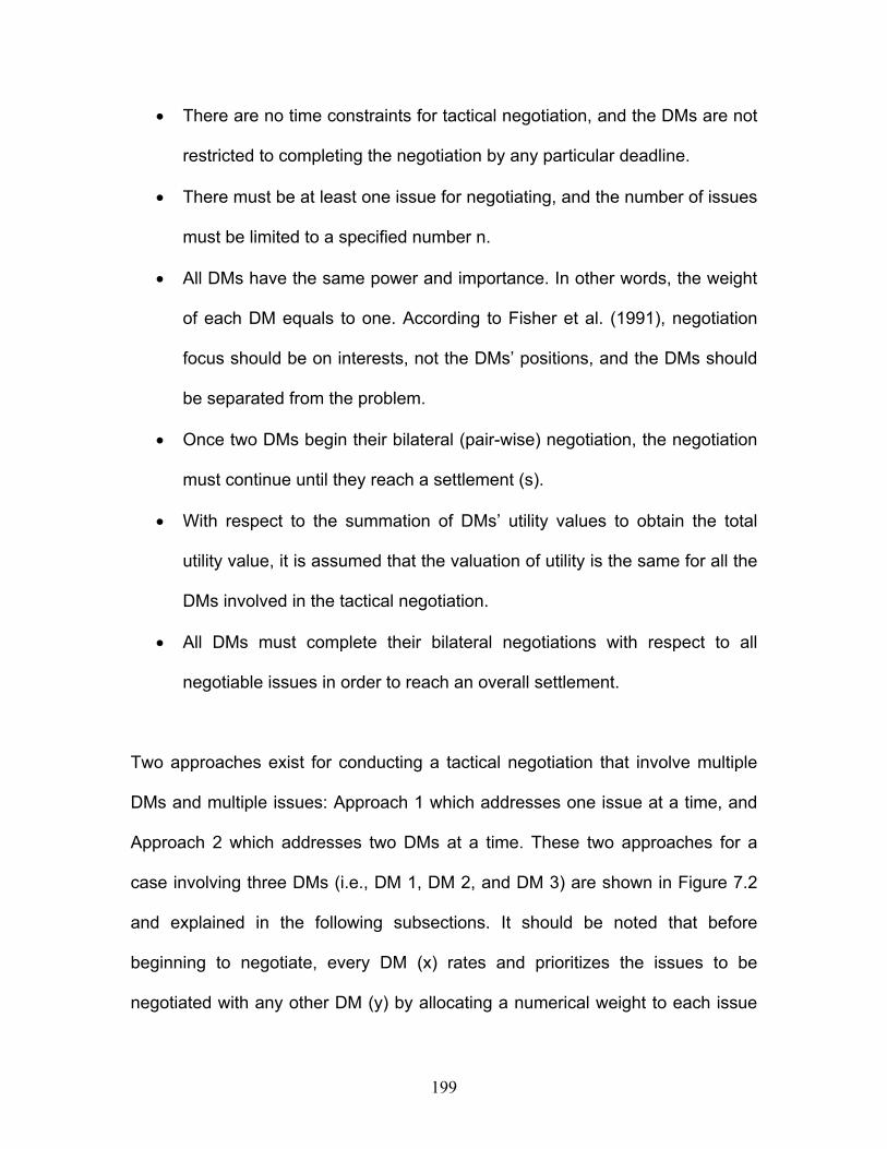
199
• There are no time constraints for tactical negotiation, and the DMs are not
restricted to completing the negotiation by any particular deadline.
• There must be at least one issue for negotiating, and the number of issues
must be limited to a specified number n.
• All DMs have the same power and importance. In other words, the weight
of each DM equals to one. According to Fisher et al. (1991), negotiation
focus should be on interests, not the DMs’ positions, and the DMs should
be separated from the problem.
• Once two DMs begin their bilateral (pair-wise) negotiation, the negotiation
must continue until they reach a settlement (s).
• With respect to the summation of DMs’ utility values to obtain the total
utility value, it is assumed that the valuation of utility is the same for all the
DMs involved in the tactical negotiation.
• All DMs must complete their bilateral negotiations with respect to all
negotiable issues in order to reach an overall settlement.
Two approaches exist for conducting a tactical negotiation that involve multiple
DMs and multiple issues: Approach 1 which addresses one issue at a time, and
Approach 2 which addresses two DMs at a time. These two approaches for a
case involving three DMs (i.e., DM 1, DM 2, and DM 3) are shown in Figure 7.2
and explained in the following subsections. It should be noted that before
beginning to negotiate, every DM (x) rates and prioritizes the issues to be
negotiated with any other DM (y) by allocating a numerical weight to each issue

200
(i). Thus, the greater the weight value of an issue, the more important the issue is
for a DM, provided that 0 ≤ wxy(i) ≤ 1 and ∑=
=n
iixyw
1)( 1 , where n is the total number
of issues. Some studies (Alfares and Duffuaa, 2008; Belton and Stewart, 2001;
Keeney and Raiffa, 1976; Lootsma, 1999; Saaty, 1980, 1990, 1994) have been
conducted with the goal of determining proper numerical values for the weights of
the issues.
7.3.1. Approach 1: One Issue at a Time
With this approach, DMs conduct a pair-wise negotiation with respect to one
issue at a time (e.g., DM 1 - DM 2; DM 1 - DM 3; etc.) until a settlement point
(s12, s13) is reached. When every DM conducts its pair-wise negotiation with other
DM 1 DM 2 u12
s12
Issue 1 Issue 2 Issue n
….
DM1 DM2
u12
s12
DM1
DM2 u12
s12
DM 1 DM 3 u13
s13
DM2 DM3 u23
s23
….
Approach 2: Two DMs at a Time A
pproach 1: One Issue at a T
ime
Figure 7.2: Two Approaches for Conducting Tactical Negotiation

201
DMs with respect to Issue 1, an average settlement point (Sissue1) can be
determined for every DM. Upon completing the pair-wise negotiations for Issue 1,
the DMs then begin pair-wise negotiations for Issue 2, and an average settlement
point (Sissue2) is also calculated for each DM. This negotiation process continues
until the DMs involved reach mutual agreement (i.e., an average settlement
point) with respect to all the negotiation issues.
The above negotiating process is used for a situation in which three DMs are
involved in tactical negotiations with respect to multiple issues. The average
settlement point for each DM that results from negotiating issue i is determined
using the following equations:
2
)]()([ 131312121
iissueiissueiissueiissueiissueDM
swswS −−−−−−−−
−−
+= [2]
2
)]()([ 232321212
iissueiissueiissueiissueiissueDM
swswS −−−−−−−−
−−
+= [3]
2
)]()([ 313131313
iissueiissueiissueiissueiissueDM
swswS −−−−−−−−
−−
+= [4]
where: SDM1-issue-i: DM 1’s average settlement point resulting from negotiating issue i w12-issue-i: DM 1’s weight for issue i when negotiating with DM 2 s12-issue-i: DM 1’s settlement point resulting from negotiating with DM 2 w13-issue-i: DM 1’s weight for issue i when negotiating with DM 3 s13-issue-i: DM 1’s settlement point resulting from negotiating with DM 3
The above settlement points represent the amount of concession that each DM
should make to reach agreement about issue i. To determine the average
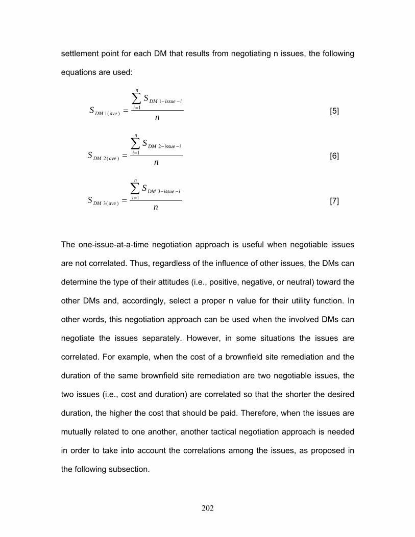
202
settlement point for each DM that results from negotiating n issues, the following
equations are used:
n
SS
n
iiissueDM
aveDM
∑=
−−
= 11
)(1 [5]
n
SS
n
iiissueDM
aveDM
∑=
−−
= 12
)(2 [6]
n
SS
n
iiissueDM
aveDM
∑=
−−
= 13
)(3 [7]
The one-issue-at-a-time negotiation approach is useful when negotiable issues
are not correlated. Thus, regardless of the influence of other issues, the DMs can
determine the type of their attitudes (i.e., positive, negative, or neutral) toward the
other DMs and, accordingly, select a proper n value for their utility function. In
other words, this negotiation approach can be used when the involved DMs can
negotiate the issues separately. However, in some situations the issues are
correlated. For example, when the cost of a brownfield site remediation and the
duration of the same brownfield site remediation are two negotiable issues, the
two issues (i.e., cost and duration) are correlated so that the shorter the desired
duration, the higher the cost that should be paid. Therefore, when the issues are
mutually related to one another, another tactical negotiation approach is needed
in order to take into account the correlations among the issues, as proposed in
the following subsection.

203
7.3.2. Approach 2: Two DMs at a Time
With this approach, as shown in Figure 7.2, two pairs of DMs (e.g., DM 1 - DM 2;
DM 3 - DM 4) conduct pair-wise negotiations with respect to all the issues at a
time and continue their negotiation until a settlement point is reached with
respect to every issue. In contrast with the first approach, the correlations among
the issues influence the selection of the n value for the DMs’ utility function. In
other words, the n values selected for two the DMs’ utility functions for
negotiating issue i using Approach 1 are different from the n values selected for
the same DMs and the same issue when Approach 2 is used. Different
settlement points may therefore result from using different approaches.
Once the two DMs complete their negotiations for all issues, each DM will start
pair-wise negotiation with another DM (e.g., DM 1 - DM 3; DM 2 - DM 4) for all
issues. With this approach, two DMs may negotiate the issues one by one, or
they may negotiate all issues simultaneously. The advantage of this approach is
that it takes into account the correlations among the issues. The negotiation
process is complete when every DM has completed its pair-wise negotiation with
all the other DMs.
This negotiating process is used for a situation in which three DMs are involved
and two DMs conduct a pair-wise negotiation for n issues at a time. The average
settlement point for each DM is then determined using the following equations:

204
n
swswS
n
iiissue
n
iiissue
aveDM 2
)()(1
13131
1212
)(1
⎥⎦
⎤⎢⎣
⎡×+⎥
⎦
⎤⎢⎣
⎡×
=∑∑=
−=
−
[8]
n
swswS
n
iiissue
n
iiissue
aveDM 2
)()(1
23231
2121
)(2
⎥⎦
⎤⎢⎣
⎡×+⎥
⎦
⎤⎢⎣
⎡×
=∑∑=
−=
−
[9]
n
swswS
n
iiissue
n
iiissue
aveDM 2
)()(1
32321
3131
)(3
⎥⎦
⎤⎢⎣
⎡×+⎥
⎦
⎤⎢⎣
⎡×
=∑∑=
−=
−
[10]
where: SDM1(ave): DM 1’s average settlement point resulted from negotiating n issues SDM2(ave): DM 2’s average settlement point resulted from negotiating n issues SDM3(ave): DM 3’s average settlement point resulted from negotiating n issues w12-issue-i: DM 1’s weight for issue i when negotiating with DM 2 w21-issue-i: DM 2’s weight for issue i when negotiating with DM 1 w13-issue-i: DM 1’s weight for issue i when negotiating with DM 3 w31-issue-i: DM 3’s weight for issue i when negotiating with DM 1 w23-issue-i: DM 2’s weight for issue i when negotiating with DM 3 w32-issue-i: DM 3’s weight for issue i when negotiating with DM 2 s12-issue-i: DM 1’s settlement point resulting from negotiating with DM 2 s21-issue-i: DM 2’s settlement point resulting from negotiating with DM 1 s13-issue-i: DM 1’s settlement point resulting from negotiating with DM 3 s31-issue-i: DM 3’s settlement point resulting from negotiating with DM 1 s23-issue-i: DM 2’s settlement point resulting from negotiating with DM 3 s32-issue-i: DM 3’s settlement point resulting from negotiating with DM 2 n: number of issues
It should be noted that the set of equations [8], [9], [10] and the set of equations
[5], [6], [7] result in the same values for the settlement point only when all issues
are negotiated by the DMs. Therefore, when all issues are negotiated, either set
can be used to determine the average settlement point for each DM. It should
205
also be mentioned that equations [8], [9], and [10] are used only when the DMs
conduct pair-wise negotiations for all issues. If two DMs negotiate only some of
the issues, then equations [2], [3], [4], [5], [6], and [7] must be used in order to
determine the average settlement point with respect to each DM.
The application of the two proposed approaches depends on the negotiation
situations, the DMs’ attitudes toward the other DMs, and the negotiation issues.
Although the first negotiation approach (one issue at a time) is fast and easy to
conduct among multiple DMs, the second approach (two DMs at a time), while
lengthy, is more accurate because the correlations among the issues can be
considered. The latter approach is particularly useful when the issues are
monetarily related to one another. Because the tactical negotiations for the
present case study deal with cost-based issues, the second approach was used
in order to consider the correlation of the issues, as explained in the next section.
7.4 Application to the School of Pharmacy Tactical Negotiation
The process of tactical negotiation involving multiple DMs and multiple issues, as
proposed in the previous section, was implemented, as discussed in this section,
in order to develop a tactical negotiation methodology for the UW School of
Pharmacy case study. It should be remembered that a strategic decision had
already been agreed upon by the DMs involved using the strategic negotiation
methodology presented in Chapter 5. The proposed tactical negotiation
methodology complements this strategic negotiation methodology.
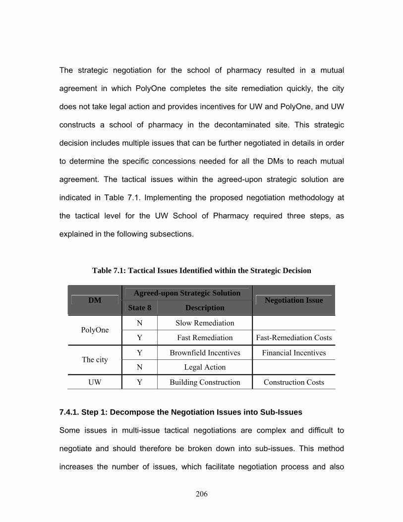
206
The strategic negotiation for the school of pharmacy resulted in a mutual
agreement in which PolyOne completes the site remediation quickly, the city
does not take legal action and provides incentives for UW and PolyOne, and UW
constructs a school of pharmacy in the decontaminated site. This strategic
decision includes multiple issues that can be further negotiated in details in order
to determine the specific concessions needed for all the DMs to reach mutual
agreement. The tactical issues within the agreed-upon strategic solution are
indicated in Table 7.1. Implementing the proposed negotiation methodology at
the tactical level for the UW School of Pharmacy required three steps, as
explained in the following subsections.
Table 7.1: Tactical Issues Identified within the Strategic Decision
7.4.1. Step 1: Decompose the Negotiation Issues into Sub-Issues
Some issues in multi-issue tactical negotiations are complex and difficult to
negotiate and should therefore be broken down into sub-issues. This method
increases the number of issues, which facilitate negotiation process and also
Agreed-upon Strategic Solution DM
State 8 Description Negotiation Issue
N Slow Remediation PolyOne
Y Fast Remediation Fast-Remediation Costs
Y Brownfield Incentives Financial Incentives The city
N Legal Action
UW Y Building Construction Construction Costs

207
helps the DMs prioritize their issues for negotiation. Keeney (1992) believed that
breaking down the issues into sub-issues allows the involved DMs to solve the
least complicated issues first, and they will then be more engaged and
encouraged to negotiate the remaining issues. Bellucci and Zeleznikow (2005)
also recognized that there may be sub-issues within the issues on which
agreement can be attained. Each sub-issue can also be decomposed into other
sub-issues so that a hierarchy of issues and sub-issues is formed. It is important
to note that the larger the number of issues in negotiation, the easier it may be to
allocate them, since the possibility of trade-offs between the issues increases.
However, decomposing a negotiable issue depends on the negotiation
conditions, and there are cases in which an issue can not be decomposed into
sub-issues. Figure 7.3 shows a flowchart of the issues and sub-issues identified
for the school of pharmacy case study.
Negotiable Issue
Sub-issue 1 Cannibalize remaining facilities
Sub-issue 2 Demolish & remove old structures
Sub-issue 3Environmental
remediation
Sub-issue 4Write-off back taxes & charges
Sub-issue 5 Reimburse for maintenance
expenses
Figure 7.3: The Hierarchy of Issues for the School of Pharmacy Negotiations
Sub-issue 6Initial
construction costs
Issue 2 Financial Incentives
Issue 3 Construction Costs
Issue 1 Fast-Remediation Costs
208
According to the agreed-upon strategic solution (Table 7.1), PolyOne agreed to
remediate the site fast, and thus PolyOne’s negotiable issue is the fast-
remediation cost. In other words, because extra costs were involved in fast
remediation, PolyOne intended to negotiate the extra costs with the other DMs
with a view to determining how much the other DMs would be able to help. The
process of fast site remediation consists of three steps: 1) cannibalize the
remaining facilities (i.e., take salvageable parts of disabled machines or facilities
and use them in building or repairing other equipment or facilities); 2) demolish
and remove the old buildings; and 3) perform the environmental remediation.
Therefore, as shown in Figure 7.3, fast-remediation costs can be broken down
into three cost-related sub-issues that correspond to these three steps.
The city’s issue was brownfield incentives, which consisted of two sub-issues: 1)
write off the back taxes and unpaid charges, and 2) reimburse the other DMs for
maintenance expenses. Because of the threats to environment and the health
hazards, the city, as a municipal organization, was the most cooperative DM
because of the need to make sure that the contaminated site was redeveloped
as soon as possible. Therefore, the city intended to provide incentives for the
other DMs who were faced with financial difficulties. Due to the huge amount of
unpaid charges that had been accumulated because the contaminated site had
been abandoned for such a long time, the city was engaged in tactical
negotiations with the other DMs in order to pay (i.e., write off) some of the unpaid
charges and taxes that were owed to the city. There was also conflict about the
209
site maintenance expenses, and the city was involved in detailed negotiation to
pay (i.e., reimburse) a reasonable amount of the expenses to the other DMs.
Finally, UW’s negotiation issue was the initial construction costs. Although UW
was the primarily responsible for constructing the school of pharmacy, some of
the initial construction activities were costly, and UW needed financial help from
the other DMs. Therefore, UW was engaged in pair-wise negotiations with the
other DMs with respect to the initial construction costs.
7.4.2. Step 2: Identify the DMs’ Least Expectations
Prior to the start of a tactical negotiation, the involved DMs identify their minimum
expectation with respect to each issue. The minimum expectation in tactical
negotiation is referred to as the disagreement point (d) which represents each
DM’s minimum level of satisfaction on which the DMs count if they do not reach
any agreement. The individual rationality condition is that no DM receives less
satisfaction than he or she would receive at point d (Kilgour 2006). It is thus
guaranteed that the DMs can achieve at least d. Therefore, to maximize their
negotiation position, every DM considers the other DMs and the negotiable
issues, and attempts to find a disagreement point before the beginning of a pair-
wise negotiation. For example, when the city and PolyOne negotiate the extra
cost (e.g., $1,000,000) associated with the fast site remediation, the city may not
accept more than a 60% concession, or $600,000, which represents the city’s

210
disagreement point. In other words, the city will not accept any tactical solution
that requires a payment greater than $600,000.
7.4.3. Step 3: Simulate the Tactical Negotiation
With respect to the tactical negotiation approaches proposed in Figure 7.2, the
two-DMs-at-a-time negotiation approach was employed in order to simulate the
tactical negotiations for the school of pharmacy. Because the issues in this case
study are monetarily and mutually related to one another, the selected approach
is more suitable for considering the interrelationships between the issues and the
correlation among the sub-issues. The simulated tactical negotiation
methodology for the school of pharmacy is shown in Figure 7.4.
As can be seen, the DMs first consider the correlations among the issues and
accordingly determine the weight of the issues as well as their minimum
expectation (i.e., the disagreement point) with respect to each issue. The DMs
then conduct pair-wise negotiation only for the issues that relate to both DMs,
and therefore, they do not negotiate for the issues related to the third DM. For
example, PO and UW will not conduct pair-wise negotiations for sub-issues 4
and 5, which are the city’s issues (Figure 7.4). Also, there is no single issue to be
negotiated by all the DMs. In this case study, three sets of pair-wise negotiations
were conducted: between PO-City, PO-UW, and the City-UW. The three sets of
negotiations are described in the following subsections.
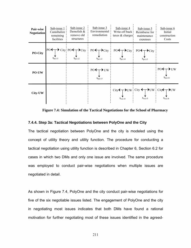
211
7.4.4. Step 3a: Tactical Negotiations between PolyOne and the City
The tactical negotiation between PolyOne and the city is modeled using the
concept of utility theory and utility function. The procedure for conducting a
tactical negotiation using utility function is described in Chapter 6, Section 6.2 for
cases in which two DMs and only one issue are involved. The same procedure
was employed to conduct pair-wise negotiations when multiple issues are
negotiated in detail.
As shown in Figure 7.4, PolyOne and the city conduct pair-wise negotiations for
five of the six negotiable issues listed. The engagement of PolyOne and the city
in negotiating most issues indicates that both DMs have found a rational
motivation for further negotiating most of these issues identified in the agreed-
PO City
Sub-issue 1 Cannibalize remaining facilities
Sub-issue 2 Demolish & remove old structures
Figure 7.4: Simulation of the Tactical Negotiations for the School of Pharmacy
PO-UW
City-UW
Sub-issue 3 Environmental
remediation
Sub-issue 4 Write-off back taxes & charges
Sub-issue 5 Reimburse formaintenance
expenses
PO-City spc) i1
Sub-issue 6 Initial
construction Costs
PO City
spc) i2
PO City
spc) i3
PO City
spc) i4
PO City
spc) i5
PO UW
spu) i3
PO UW
spu) i6
City UW
scu) i6
City UW
scu) i4
Pair-wise Negotiation
City UW
scu) i5

212
upon strategic solution. The background of this case study also indicates that the
city and PolyOne participated in many rounds of negotiations and meetings to
determine each DM’s share of the costs of remediation of the brownfield site.
The pair-wise negotiation begins with the two DMs first evaluating all the issues
and determining the weight and the disagreement point, or the minimum
expectation, with respect to each negotiable issue. They then take into account
the correlations among the issues to discuss whether they can make more
concessions with respect to one issue in order to receive more benefits with
respect to another issue. In other words, understanding the relationship between
issues allows the DMs to find the most suitable range of concessions (i.e., an
appropriate n value for the utility function) they can make in order to reach a
more stable agreement. Understanding the interrelationships among the issues
also helps the DMs to adjust their attitudes during their pair-wise negotiations.
After determining the preliminary considerations, such as the weight of issues
and the disagreement points, an appropriate utility function form is assigned to
each DM for each issue, and an integrated utility function is then developed. The
maximum point on the integrated utility function represents the highest level of
satisfaction in a joint decision and also represents the settlement point which
represents the concessions the DMs need to make in order to reach mutual
agreement with respect to each issue. The five pair-wise negotiations between
PolyOne and the city were simulated as shown in Figure 7.5.

213
CityPO
Integrated
0102030405060708090
100110120130140150160170180190200210
0 10 20 30 40 50 60 70 80 90 100
Concession (%)
Util
ity (%
)
(Max. Utility)
b) Sub-issue 2: Demolish & Remove Old Structures
40% of the cost of demolishing old structures is paid by City
PO : n = 8 (positive attitude)City: n = 4 (positive attitude)
CityPO
Integrated
0102030405060708090
100110120130140150160170180190200210
0 10 20 30 40 50 60 70 80 90 100Concession (%)
Util
ity (%
)
(Max. Utility)
d) Sub-issue 4: Write-off Back Taxes & Charges
50% of the back taxes are written off by City
PO : n = 5 (positive attitude)City: n = 5 (positive attitude)
CityPO
Integrated
0102030405060708090
100110120130140150160170180190200210
0 10 20 30 40 50 60 70 80 90 100
Concession (%)
Util
ity (%
)
(Max. Utility)
a) Sub-issue 1: Cannibalize Remaining Facilities
60% of the cost of cannibalizing is paid by City
PO : n = 3 (positive attitude)City: n = 7 (positive attitude)
CityPO
Integrated
0102030405060708090
100110120130140150160170180190200
0 10 20 30 40 50 60 70 80 90 100
Concession (%)
Util
ity (%
)
(Max. Utility)
c) Sub-issue 3: Environmental Remediation
30% of the cost of environmental remediation is paid by City
PO : n = 9 (positive attitude)City: n = 2 (positive attitude)
CityPO
Integrated
0102030405060708090
100110120130140150160170180
0 10 20 30 40 50 60 70 80 90 100
Concession (%)
Util
ity (%
)
(Max. Utility)
e) Sub-issue 5: Reimburse for Maintenance Expenses
PO : n = 1 (neutral attitude)City: n = 9 (positive attitude)
80% of the maintenance cost is paid by City
Figure 7.5: Tactical Negotiations between PolyOne and the City
))(100( 1)(
nnPolyOne xU −=
nnCity xU )100)(100( 1
)( −= −

214
It can be noted that the utility functions, shown in Figure 7.5, were selected for
PolyOne and the city in which x represents the amount of the concessions made
by the DMs and n represents the power term of the utility function.
7.4.5. Step 3b: Tactical Negotiations between PolyOne and UW
PolyOne and UW had two negotiable issues: 1) the cost of the environmental
remediation, and 2) the initial cost of constructing the UW school of pharmacy. In
this case study, the site was transferred to UW as the new owner of the site. As
PolyOne negotiated the cost of the environmental remediation with the city, as
discussed in the previous subsection, PolyOne was also willing to negotiate
some of the remediation costs with UW. Because a lengthy remediation process
would continued beyond the point at which UW became the site owner, UW did
not want any interruption in the remediation process established by PolyOne, and
UW was therefore engaged in the negotiation process.
With respect to the third issue, the initial construction costs, UW was the DM
mainly responsible for the costs of construction. However, because PolyOne had
already assembled a great deal of suitable construction equipment on the site,
UW was willing to negotiate the costs of the initial construction activities with
PolyOne. The activities were overlapped with the PolyOne’s construction
activities. The two pair-wise negotiations between PlyOne and UW are modeled
as shown in Figure 7.6. The following utility functions were selected for PolyOne
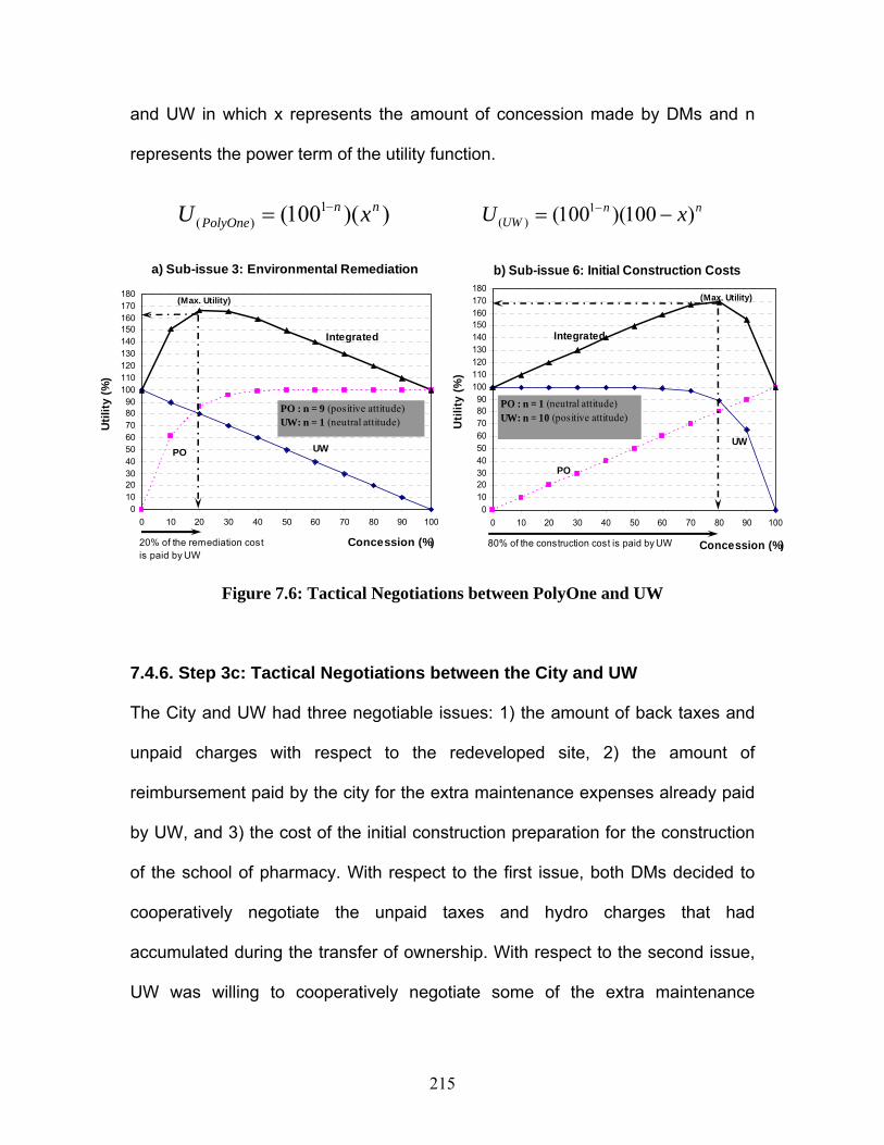
215
UWPO
Integrated
0102030405060708090
100110120130140150160170180
0 10 20 30 40 50 60 70 80 90 100
Concession (%)
Util
ity (%
)
(Max. Utility)
a) Sub-issue 3: Environmental Remediation
PO : n = 9 (positive attitude)UW: n = 1 (neutral attitude)
20% of the remediation cost is paid by UW
UW
PO
Integrated
0102030405060708090
100110120130140150160170180
0 10 20 30 40 50 60 70 80 90 100
Concession (%)
Util
ity (%
)
(Max. Utility)
b) Sub-issue 6: Initial Construction Costs
PO : n = 1 (neutral attitude)UW: n = 10 (positive attitude)
80% of the construction cost is paid by UW
and UW in which x represents the amount of concession made by DMs and n
represents the power term of the utility function.
Figure 7.6: Tactical Negotiations between PolyOne and UW
7.4.6. Step 3c: Tactical Negotiations between the City and UW
The City and UW had three negotiable issues: 1) the amount of back taxes and
unpaid charges with respect to the redeveloped site, 2) the amount of
reimbursement paid by the city for the extra maintenance expenses already paid
by UW, and 3) the cost of the initial construction preparation for the construction
of the school of pharmacy. With respect to the first issue, both DMs decided to
cooperatively negotiate the unpaid taxes and hydro charges that had
accumulated during the transfer of ownership. With respect to the second issue,
UW was willing to cooperatively negotiate some of the extra maintenance
))(100( 1)(
nnPolyOne xU −= nn
UW xU )100)(100( 1)( −= −
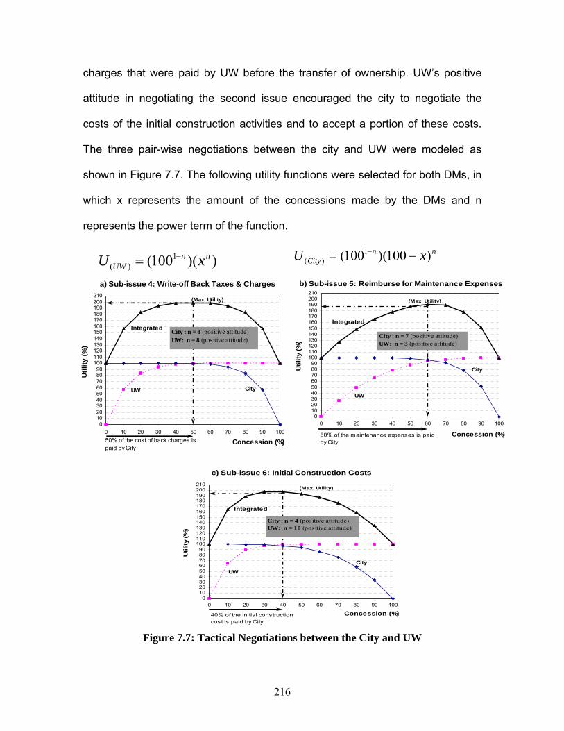
216
CityUW
Integrated
0102030405060708090
100110120130140150160170180190200210
0 10 20 30 40 50 60 70 80 90 100
Concession (%)
Util
ity (%
)
(Max. Utility)
a) Sub-issue 4: Write-off Back Taxes & Charges
City : n = 8 (positive attitude)UW: n = 8 (positive attitude)
50% of the cost of back charges is paid by City
City
UW
Integrated
0102030405060708090
100110120130140150160170180190200210
0 10 20 30 40 50 60 70 80 90 100
Concession (%)
Util
ity (%
) (Max. Utility)
b) Sub-issue 5: Reimburse for Maintenance Expenses
City : n = 7 (positive attitude)UW: n = 3 (positive attitude)
60% of the maintenance expenses is paid by City
City
UW
Integrated
0102030405060708090
100110120130140150160170180190200210
0 10 20 30 40 50 60 70 80 90 100
Concession (%)
Util
ity (%
)
(Max. Utility)
c) Sub-issue 6: Initial Construction Costs
City : n = 4 (positive attitude)UW: n = 10 (positive attitude)
40% of the initial constructioncost is paid by City
charges that were paid by UW before the transfer of ownership. UW’s positive
attitude in negotiating the second issue encouraged the city to negotiate the
costs of the initial construction activities and to accept a portion of these costs.
The three pair-wise negotiations between the city and UW were modeled as
shown in Figure 7.7. The following utility functions were selected for both DMs, in
which x represents the amount of the concessions made by the DMs and n
represents the power term of the function.
Figure 7.7: Tactical Negotiations between the City and UW
nnCity xU )100)(100( 1
)( −= −))(100( 1
)(nn
UW xU −=
217
7.4.7. Discussion of the Tactical Negotiation Results
As described in the previous subsections, the tactical negotiation methodology
involving six issues and three DMs (i.e., PolyOne, the city, and UW) was
developed for the present case study. The concept of utility function was used to
model and illustrate the pair-wise negotiations between PolyOne - City, PolyOne
- UW, and City – UW, as set out in Subsections 7.4.4, 7.4.5, and 7.4.6,
respectively. In this subsection, the outcomes resulting from the tactical
negotiations are summarized as shown in Table 7.2, and a brief discussion of the
results is provided as follows.
As previously explained, after mutually agreeing on a strategic decision, the
involved DMs continued their tactical negotiations very cooperatively and
preferred to avoid any negative attitudes toward one another during the
negotiations. The DMs realized that negative attitudes are not beneficial and
would threaten the agreed-upon strategic solution which had been achieved after
many years of intensive meetings and negotiations. Accordingly, when the DMs’
tactical negotiations were modeled using utility function, the n values (i.e., the
power term of the utility functions) selected for the DMs were equal to or greater
than one, which means that each DM’s attitude toward the other DMs was either
neutral or positive. The city, PolyOne, and UW all had a positive attitude except
in three situations in which PolyOne and UW had neutral attitudes toward other
DM during their pair-wise negotiations, as shown in Table 7.2.
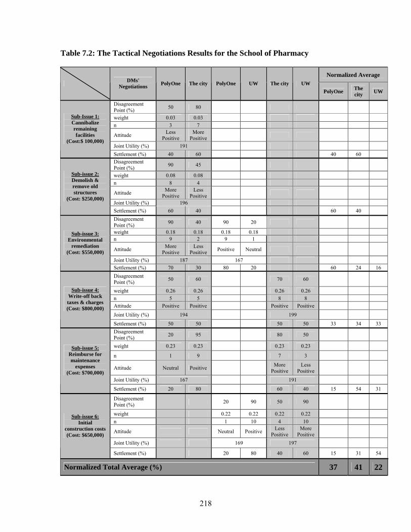
218
Table 7.2: The Tactical Negotiations Results for the School of Pharmacy
Normalized Average DMs'
Negotiations PolyOne The city PolyOne UW The city UW PolyOne The
city UW
Disagreement Point (%) 50 80
weight 0.03 0.03 n 3 7
Attitude Less Positive
More Positive
Joint Utility (%) 191
Sub-Issue 1: Cannibalize remaining facilities
(Cost:$ 100,000)
Settlement (%) 40 60 40 60 Disagreement Point (%) 90 45
weight 0.08 0.08 n 8 4
Attitude More Positive
Less Positive
Joint Utility (%) 196
Sub-issue 2: Demolish & remove old structures
(Cost: $250,000)
Settlement (%) 60 40 60 40 Disagreement Point (%) 90 40 90 20
weight 0.18 0.18 0.18 0.18 n 9 2 9 1
Attitude More Positive
Less Positive Positive Neutral
Joint Utility (%) 187 167
Sub-issue 3: Environmental
remediation (Cost: $550,000)
Settlement (%) 70 30 80 20 60 24 16 Disagreement Point (%) 50 60 70 60
weight 0.26 0.26 0.26 0.26 n 5 5 8 8 Attitude Positive Positive Positive Positive
Joint Utility (%) 194 199
Sub-issue 4: Write-off back taxes & charges (Cost: $800,000)
Settlement (%) 50 50 50 50 33 34 33 Disagreement Point (%) 20 95 80 50
weight 0.23 0.23 0.23 0.23
n 1 9 7 3
Attitude Neutral Positive More Positive
Less Positive
Joint Utility (%) 167 191
Sub-issue 5: Reimburse for maintenance
expenses (Cost: $700,000)
Settlement (%) 20 80 60 40 15 54 31
Disagreement Point (%) 20 90 50 90
weight 0.22 0.22 0.22 0.22 n 1 10 4 10
Attitude Neutral Positive Less Positive
More Positive
Joint Utility (%) 169 197
Sub-issue 6: Initial
construction costs (Cost: $650,000)
Settlement (%) 20 80 40 60 15 31 54
Normalized Total Average (%) 37 41 22
219
The six negotiation issues and their approximate costs are shown in the first
column on the left in Table 7.2. The input information (e.g., disagreement point,
weight) and the output results (e.g., joint utility, settlement) are shown in the
second column from the left in Table 7.2. The two rows at the bottom of the table
display the suggested average share that each DM should pay with respect to
the total cost of the six issues.
The final results of the tactical negotiation (the last row in Table 7.2) indicate that
the city agrees to pay a greater share of the total cost (37%) than either PolyOne
(33%), or UW (30%). The results are consistent with the real-life detailed
negotiations that took place. One of the main responsibilities of the City of
Kitchener, as a municipal organization, is to remediate and redevelop brownfield
sites as quickly as possible. The City of Kitchener (the city) was particularly very
cooperative during the tactical negotiations and did not even prefer to have
neutral attitudes toward PolyOne and UW, in the hope of helping the other DMs
to reach a stable solution after the lengthy negotiations.
With respect to the City-PolyOne pair-wise negotiations, both DMs considered
the preconditions of the negotiation, assessed the correlations among the
negotiating issues, and decided to negotiate five issues as, listed in Table 7.2.
Negotiation of the first issue (i.e., cannibalize the remaining facilities) took place
only between the city and PolyOne since UW was not involved with that issue.
When the fast site remediation was decided on at the strategic level, PolyOne

220
preferred to reuse some of the existing facilities, and therefore, the process of
cannibalization was considered. PolyOne negotiated the cost of the process
($100,000) with the city. The results of the negotiation of the demolition and
removal of the old structure on the contaminated site (issue 2) was that PolyOne
pays 60% of the cost and the city pays 40% of the cost because some of the old
structures and equipment belonged to the city and it was the city’s responsibility
to contribute to the cost. Both DMs conducted a very successful tactical
negotiation with respect to this issue and reached a higher level of satisfaction
(joint utility of 196) than they achieved with respect to their other issues (Table
7.2). On the other hand, in negotiating the issue of reimbursing for maintenance
expenses (issue 5), both DMs reached the lowest level of satisfaction (joint utility
of 167). This low level is due mainly to the fact that although the city had a
positive attitude toward its opponent, PolyOne had a neutral attitude toward the
city, which caused the lower level of joint satisfaction.
With respect to the PolyOne-UW bilateral negotiations, both DMs reviewed the
available negotiation issues and agreed to negotiate two of them, as shown in
Table 7.2. In negotiating the issue of environmental remediation (issue 3), UW
preferred to negotiate the issue with PolyOne because the lengthy process of
remediation had been continued during the period when UW was the new owner
of the site. The outcome of the negotiation was that 20% of the cost is to be paid
by UW. UW’s cooperative attitude in negotiating the cost of the remediation
encouraged PolyOne to accept UW’s request to negotiate the initial costs of the

221
construction of the school of pharmacy, for which UW was mainly responsible.
Therefore, PolyOne negotiated with UW, having a neutral attitude toward UW,
and agreed to share 20% of the cost according to the negotiation outcome.
With respect to the City-UW bilateral negotiations, both DMs reviewed the
available negotiation issues and preferred to negotiate the costs of three issues:
1) write off back taxes and unpaid charges, 2) provide reimbursement for the site
maintenance expenses, and 3) contribute to the costs of initial construction
activities. Both the city and UW held very successful negotiations with respect to
the unpaid charges for the abandoned site, and for the cost of the initial
construction activities. In particular, the highest level of satisfaction (joint utility of
199) was achieved when both DMs very positively negotiated the cost of the
back taxes and previous charges (Table 7.2). One of the reasons for such a high
level of cooperation between the city and UW is that when construction of an
educational building on the remediated site was agreed upon, the city realized
that the sooner the building could be constructed, the more benefits downtown
Kitchener businesses will gain. In other words, the city envisioned the
cooperative tactical negotiation with UW as a beneficial investment for the
taxpayers, who were asking for a better business in downtown Kitchener. Using
the proposed tactical negotiation methodology, each DM’s share of the costs with
respect to each issue is listed in Table 7.3. The tactical negotiation issues and
their associated costs are shown in the two columns at the left in Table 7.3. The
percentage share and corresponding monetary share of the costs with respect to

222
each DM are also displayed in Table 7.3. The results shown in Table 7.3 are the
exact amount of the concessions that must be made by the DMs in order for
them to reach mutual agreement at the tactical level of negotiation in this case
study. In other words, to complement the strategic negotiation and to complete
the negotiation process for the case study, the concessions proposed in Table
7.3 should be made by the DMs involved in the brownfield negotiation.
Table 7.3: DMs’ Shares of the Costs of the Tactical Issues
The resulting sharing of the costs on the part of the DMs involved in the tactical
negotiations of the school of pharmacy lead to the following considerations:
1. With respect to the total cost of all six issues ($3,050,000), the city will pay
the largest share ($1,143,500), followed by PolyOne with the second
largest share ($986,500), and UW, with the third largest share ($920,000).
DM’s Share (%) DM’s Share ($) Sub-issue Cost ($)
PolyOne The city UW PolyOne The city UW
1 100,000 40 60 40,000 60,000
2 250,000 60 40 150,000 100,000
3 550,000 60 24 16 330,000 132,000 88,000
4 800,000 33 34 33 264,000 272,000 264,000
5 700,000 15 54 31 105,000 378,000 217,000
6 650,000 15 31 54 97,500 201,500 351,000
Average 508,333 37 41 22 164,400 190,600 153,300
Total ($) 3,050,000 986,500 1,143,500 920,000

223
The proposed cost sharing is consistent with the background of the
negotiation with respect to the school of pharmacy, in which the City of
Kitchener showed the highest level of cooperation along with a positive
attitude toward both PolyOne and UW. The City of Kitchener knew that
PolyOne and UW were not responsible for the whole redevelopment costs
of the brownfield site, which had been abandoned for many years.
Therefore, the city took bold action during the tactical negotiations and
accepted a large share of the costs.
2. According to the proposed results shown in Table 7.3, PO’s largest cost is
$330,000 for issue 3 (environmental remediation), the city’s largest share
is $378,000 for issue 5 (reimbursement for maintenance expenses), and
UW’s largest share is $351,000 for issue 6 (initial construction costs). The
results indicate that the three DMs were ready to negotiate and to make a
large contribution with respect to the issues that concerned them the most:
issues 3, 5, and 6 for PO, the city, and UW, respectively.
3. The amounts of the cost sharing indicate that the three DMs have
contributed fairly to the negotiation of the cost of the issues, except for
issues 1 and 2, in which UW made no contribution to the negotiations, and
PolyOne and the city were solely responsible for the costs. Because the
DMs mutually accepted the strategic solution and agreed to continue their
negotiations cooperatively at the tactical level, none of them had a
negative attitude toward the other DMs during the tactical negotiations.
The DMs preferred to complete their lengthy tactical negotiations and
224
accept the costs in order to receive the future benefits of redevelopment
and to avoid additional costs of remediation by abandoning the
contaminated site.
7.5. Attitude-Based Sensitivity Analysis
As discussed in Chapter 6, the power term (n) of utility function can represent
DMs’ attitudes toward themselves and other DMs when a utility function is used
in tactical negotiation. When 0 < n < 1, 1 < n ≤ 10, or n = 1, a DM has a negative,
positive, or neutral attitude, respectively, toward itself and/or other DMs. It was
also explained that if two DMs have less cooperative attitudes (i.e., a lower n
value is selected for their utility function), then a lower joint utility (i.e., joint
satisfaction) will result from their pair-wise negotiation.
The proposed attitude-based utility function was employed for the pair-wise
negotiations explained in Section 7.4. Before the commencement of the pair-wise
tactical negotiations, an appropriate n value was assigned to each DM’s utility
function according to the DMs’ attitudes toward itself and the other DMs. Based
on the n values assigned to the DMs’ utility functions, the outcomes of the pair-
wise negotiations were obtained, as summarized in Table 7.2.
The objective of the attitude-based sensitivity analysis presented in this section is
to assess the sensitivity of the negotiation outcomes (output information) to
changes in the n values (input variables). In other words, it is important to

225
investigate the effects of changes in the attitudes of the DMs toward the other
DMs during the pair-wise tactical negotiations. It is also important to know how
changes in attitude influence the negotiation settlement point and the level of
joint satisfaction. To achieve these objectives, the attitudes of the DMs involved
in the negotiations for the school pf pharmacy were analyzed. The outcomes
resulting from the tactical negotiations were the settlement point and the joint
utility for each issue, as shown in Figures 7.5, 7.6, and 7.7 as well as in Table
7.3. To examine the sensitivity of the output values to changes in the n value as
input data, the possible range of the DMs’ n values (0 < n ≤ 10) was considered,
and the corresponding settlement points and joint utilities were obtained.
To facilitate the analysis of the results, the set of values for each output was
plotted separately against the set of n values. Therefore, with respect to each
negotiation issue and each pair-wise negotiation, two plots have been
systematically examined: 1) the variation in the settlement point with the n value
and 2) the variation in the joint utility value with the n value. The two plots have
been developed for the three pair-wise negotiations between the DMs: pair-wise
negotiations between PolyOne and the City, pair-wise negotiations between
PolyOne and UW, and pair-wise negotiations between the City and UW. The
resulting plots of the pair-wise negotiations between PolyOne and the City are
shown in Figure 7.8, between PolyOne and UW are shown in Figure 7.9, and
between the City and UW are shown in Figure 7.10.

226
a) The impact of City's attitude changes on its concession when PO's attitude is unchanged
0102030405060708090
100
0 2 4 6 8 10
City's "n"
City
's C
once
ssio
n (%
)
Issue 1
Issue 2
Issue 3Issue 4
Issue 5
b) The impact of PO's attitude changes on its concession when City's attitude is unchanged
0102030405060708090
100
0 2 4 6 8 10PO's "n"
PO
's C
once
ssio
n (%
)
Issue 1
Issue 2
Issue 3Issue 4
Issue 5
c) The impact of City's attitude changes on its utility when PO's attitude is unchanged
0
50
100
150
200
250
0 2 4 6 8 10City's "n"
City
's U
tility
(%)
Issue 1
Issue 2
Issue 3Issue 4
Issue 5
d) The impact of PO's attitude changes on its utility when City's attitude is unchanged
0
50
100
150
200
250
0 2 4 6 8 10PO's "n"
PO
's U
tility
(%)
Issue 1
Issue 2
Issue 3Issue 4
Issue 5
Figure 7.8: Sensitivity Analysis for a Specific DM in the PolyOne – City Negotiations
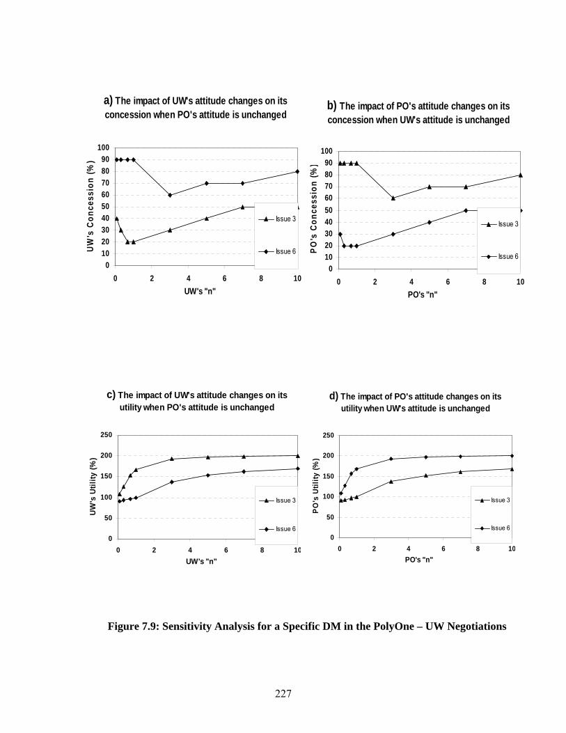
227
a) The impact of UW's attitude changes on its concession when PO's attitude is unchanged
0102030405060708090
100
0 2 4 6 8 10UW's "n"
UW's
Con
cess
ion
(%)
Issue 3
Issue 6
b) The impact of PO's attitude changes on its concession when UW's attitude is unchanged
0102030405060708090
100
0 2 4 6 8 10PO's "n"
PO's
Con
cess
ion
(%)
Issue 3
Issue 6
c) The impact of UW's attitude changes on its utility when PO's attitude is unchanged
0
50
100
150
200
250
0 2 4 6 8 10UW's "n"
UW
's U
tility
(%)
Issue 3
Issue 6
d) The impact of PO's attitude changes on its utility when UW's attitude is unchanged
0
50
100
150
200
250
0 2 4 6 8 10PO's "n"
PO's
Util
ity (%
)
Issue 3
Issue 6
Figure 7.9: Sensitivity Analysis for a Specific DM in the PolyOne – UW Negotiations
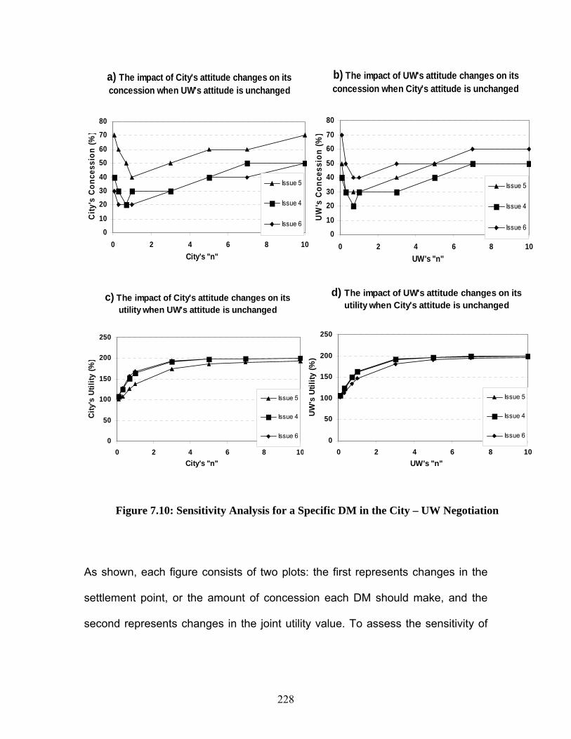
228
As shown, each figure consists of two plots: the first represents changes in the
settlement point, or the amount of concession each DM should make, and the
second represents changes in the joint utility value. To assess the sensitivity of
a) The impact of City's attitude changes on its concession when UW's attitude is unchanged
0
10
20
30
40
50
60
70
80
0 2 4 6 8 10City's "n"
City
's C
once
ssio
n (%
)
Issue 5
Issue 4
Issue 6
b) The impact of UW's attitude changes on its concession when City's attitude is unchanged
0
10
20
30
40
50
60
70
80
0 2 4 6 8 10UW's "n"
UW
's C
once
ssio
n (%
)
Issue 5
Issue 4
Issue 6
c) The impact of City's attitude changes on its utility when UW's attitude is unchanged
0
50
100
150
200
250
0 2 4 6 8 10City's "n"
City
's U
tility
(%)
Issue 5
Issue 4
Issue 6
d) The impact of UW's attitude changes on its utility when City's attitude is unchanged
0
50
100
150
200
250
0 2 4 6 8 10UW's "n"
UW's
Util
ity (%
)
Issue 5
Issue 4
Issue 6
Figure 7.10: Sensitivity Analysis for a Specific DM in the City – UW Negotiation

229
the two outputs of the negotiations with respect to each DM, the n value for one
DM is changed while the other DM’s n value remained fixed.
The plots in the figures are particularly useful when the sensitivity of the output
from the negotiation for a DM is required with respect to a particular issue, as can
be illustrated by considering the pair-wise negotiation between the city and UW.
With respect to sub-issue 6 (initial construction costs), one may examine the
effect of UW’s n value changing from n = 10 to n = 1 on the settlement point and
the joint utility value. In other words, when UW’s attitude toward the city changes
from positive to neutral, the range of reduction in the settlement point and the
joint utility level can be determined. The right-hand plots in Figure 7.10 show that
when UW’s n value changes from 10 to one during the negotiation for sub-issue
6, UW’s concession is then reduced from 60 % to 40 % with respect to that issue.
The joint utility value is also reduced from 197 to 147, which indicates that the
level of joint satisfaction drops considerably when UW changes its positive
attitude to a neutral attitude toward the city.
7.5.1. Discussion of the Attitude-Based Sensitivity Results
The plots included in the previous subsection can be used to assess changes in
the negotiation parameters and can be summarized in two plots (Figure 7.11).
The overall impact of the DMs’ attitudes on their average amount of concession
is shown in Figure 7.11a, and the impact of the DMs’ attitudes on the DMs’
average level of satisfaction is shown in Figure 7.11b.

230
a) Overall Impact of DMs' Attitude on DMs' Concession
0
10
20
30
40
50
60
70
0 2 4 6 8 10
"n"
Con
cess
ion
(%)
PO-CityPO-UWCity-UW
b) Overall Impact of DMs' Attitude on DMs' Utility
0
50
100
150
200
250
0 2 4 6 8 10
"n"
Util
ity (%
)
PO-CityPO-UWCity-UW
Figure 7.11: Overall Results of the Sensitivity Analysis for the Tactical Negotiations for the School of Pharmacy

231
As shown in Figure 7.11a, when 0 < n < 1, the DMs have a negative attitude
toward themselves and/or toward the other DMs, and the amount of concession
is considerably reduced. The steep slope of the graphs in that area indicates that
the settlement point is very sensitive to the selection of an n value of 0 < n < 1 for
a DM’s utility function. When the n value changes from less than one (i.e., a
negative attitude) to a value more than one (i.e., a positive attitude), the slope of
the graphs then increases positively. The turning point on the graphs occur when
n = 1, which means that the DMs have neutral attitudes. When the DMs have a
positive attitude toward themselves and/or the other DMs (i.e., 1 < n ≤ 10), then
the slope of the graphs increases slightly. In particular, when 2 < n ≤ 6, the
increase is more than when 7 < n ≤ 10. In other words, when an n value between
2 and 6 is selected, more changes in the DMs’ amount concession can be
expected. On the other hand, when an n value between 7 and 10 is selected for
the DMs’ utility functions, no significant change in the DMs’ amount of
concession will result.
As shown in Figure 7.11b, the utility (i.e., level of joint satisfaction) of the three
pair-wise negotiations increases when the n value is increased from 0.1 to 10.
Furthermore, when 0 < n < 1, the joint utility value is low and the marginal
changes in the average utility value increase. On the other hand, when 1 < n ≤
10, the marginal changes in the joint utility value decrease although the joint
utility value itself is high. In other words, the pair-wise negotiations conducted in
the case study indicate that when two DMs with a positive attitude negotiate, the
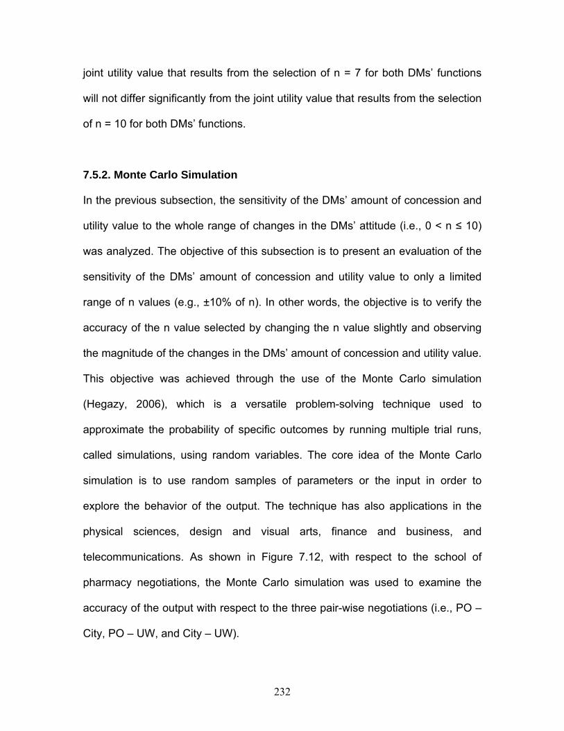
232
joint utility value that results from the selection of n = 7 for both DMs’ functions
will not differ significantly from the joint utility value that results from the selection
of n = 10 for both DMs’ functions.
7.5.2. Monte Carlo Simulation
In the previous subsection, the sensitivity of the DMs’ amount of concession and
utility value to the whole range of changes in the DMs’ attitude (i.e., 0 < n ≤ 10)
was analyzed. The objective of this subsection is to present an evaluation of the
sensitivity of the DMs’ amount of concession and utility value to only a limited
range of n values (e.g., ±10% of n). In other words, the objective is to verify the
accuracy of the n value selected by changing the n value slightly and observing
the magnitude of the changes in the DMs’ amount of concession and utility value.
This objective was achieved through the use of the Monte Carlo simulation
(Hegazy, 2006), which is a versatile problem-solving technique used to
approximate the probability of specific outcomes by running multiple trial runs,
called simulations, using random variables. The core idea of the Monte Carlo
simulation is to use random samples of parameters or the input in order to
explore the behavior of the output. The technique has also applications in the
physical sciences, design and visual arts, finance and business, and
telecommunications. As shown in Figure 7.12, with respect to the school of
pharmacy negotiations, the Monte Carlo simulation was used to examine the
accuracy of the output with respect to the three pair-wise negotiations (i.e., PO –
City, PO – UW, and City – UW).

233
The average n value was calculated for the six issues, identified in the case
study and listed in Table 7.2. A pair-wise negotiation was then simulated
between the DMs, considering the average n value for each DM’s utility function.
For each pair-wise negotiation, a settlement point and a maximum utility value
were obtained as the outputs of the negotiations before the Monte Carlo
simulation was implemented (Figure 7.12).
In the first step of evaluating the accuracy of the two results, the values within
10% of the average n value are considered, and the simulated output is obtained
for each randomly selected n value. The process is repeated 1000 times in order
to obtain 1000 sets of output which are used to determine the average of the
simulated output. The initial output is then compared with the simulated output,
and any discrepancies and errors are calculated and discussed.
nnDM xU ))(100( 1
2−=
nnDM xU )100)(100( 1
1 −= −
Input Output Function
Before Simulation
After Simulation
n (± 10 %) × n
1) Max. Utility Value 2) Settlement Point 1) Updated Utility Value 2) Updated Settlement
Point
Figure 7.12: The Application of the Monte Carlo Simulation for the Case Study

234
In the second step of evaluating the accuracy of the two results, the values within
20% of the average n value are considered, and the simulated output is obtained
for each randomly selected n value. The same process explained in the first step
is then carried out in order to obtain a different set of output. In the third and last
step, the values within 40% of the average n value are considered, the simulated
output is obtained for each randomly selected n value, and the results are
discussed. The results of the implementation of the Monte Carlo simulation in this
case study are shown in Figures 7.13, 7.14, and 7.15 for the PO – City, PO –
UW, and City – UW negotiations, respectively. The statistical results of the
simulations are also summarized in Table 7.4, followed by a brief discussion of
the simulation results.
As can be seen, the overall results of the Monte Carlo simulation indicate that no
significant change occurs in the joint utility value and the settlement point (output)
when the n value (input) changes within ± 10% and ± 20 % of the initial n value.
However, when the n value (input) changes within ± 40 % of the initial n value,
the joint utility value and the settlement point observably change. In other words,
the resulting discrepancies and errors (i.e., [initial output – simulated output] /
initial output) are very small to the point of negligible when the n value changes
within ± 10% or ± 20 %. On the other hand, the errors are relatively high when
the n value changes within ± 40%.

235
a) Within 10% of the Mean (195)
020406080
100120140160180200
187
188
189
190
191
193
194
195
196
197
199
b) Within 20% of the Mean (195)
0
50
100
150
200
250
300
350
160
164
168
172
176
180
184
188
192
196
200
c) Within 40% of the Mean (195)
050
100150200250300350400450500
53 69 85 101
117
133
149
165
181
197
213
d) Distribution of the Mean (195)
10%20%
40%
0
100
200
300
400
500
50 60 70 80 90 100 110 120 130 140 150 160 170 180 190 200 210 220
Max. Utility (Mean)
Freq
uenc
y
Figure 7.13: Histograms for PO - City Resulting from the Monte Carlo Simulation
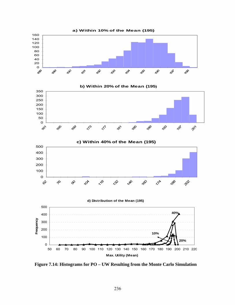
236
a) Within 10% of the Mean (195)
020406080
100120140160
188
189
190
191
192
193
194
195
196
197
198
b) Within 20% of the Mean (195)
050
100150200250300350
161
165
169
173
177
181
185
189
193
197
201
c) Within 40% of the Mean (195)
0
100
200
300
400
500
62 76 90 104
118
132
146
160
174
188
202
d) Distribution of the Mean (195)
10%
20%
40%
40%
0
100
200
300
400
500
50 60 70 80 90 100 110 120 130 140 150 160 170 180 190 200 210 220
Max. Utility (Mean)
Freq
uenc
y
Figure 7.14: Histograms for PO – UW Resulting from the Monte Carlo Simulation

237
a) Within 10% of the Mean (198)
0
50
100
150
200
250
300
192
193
193
194
195
196
197
197
198
199
200
b) Within 20% of the Mean (198)
0
50
100
150
200
250
300
184
186
187
189
190
192
194
195
197
198
200
c) Within 40% of the Mean (198)
0100200300400500600700800
86 98 110
122
134
146
158
170
182
194
206
d) Distribution of the Mean (198)
10% 20%
40%
0100200300400500600700800
50 60 70 80 90 100 110 120 130 140 150 160 170 180 190 200 210 220
Max. Utility (Mean)
Freq
uenc
y
Figure 7.15: Histograms for City – UW Resulting from the Monte Carlo Simulation
238
Table 7.4: Summary of the Monte Carlo Simulation Results for the Case Study
Simulation Simulation Statistics for Three Pair-wise Negotiations PO - City PO – UW City - UW
Settlement (%) 50 50 50
Utility 195 195 198 Before
Average “n” for Six Issues PO = 5.2 City = 5.4
PO = 5 UW = 5.5
City = 6.3 UW = 7
Settlement (%) 50 50 50
Ave. Utility (%) 195 194 198
Minimum 187 186 193
Maximum 198 198 199
Standard Deviation 1 2 1
Setl. 0 0 0
Within 10% of average “n”
Error (%) Util. 0 0.5 0
Settlement (%) 50 50 50
Ave. Utility (%) 194 193 197
Minimum 175 170 180
Maximum 199 199 200
Standard Deviation 3 4 2
Setl. 0 0 0
Within 20% of average “n”
Error (%) Util. 0.5 1.0 0.5
Settlement (%) 40 40 30
Ave. Utility (%) 187 187 192
Minimum 82 73 71
Maximum 200 200 200
Standard Deviation 18 21 16
Setl. 10 10 20
After
Within 40% of average “n”
Error (%) Util. 4.1 4.1 3.0
As shown in Table 7.4, when the n values within ± 40% are considered as the
simulation input, the standard deviation (σ) reaches 18, 21, and 16 for the PO –

239
City, PO – UW, and City – UW negotiations, respectively. Such high standard
deviations indicate that the output data are spread over a large range of the
mean value (output) as shown in Figures 7.13d, 7.14d, and 7.15d. On the other
hand, when the n values are selected within ± 10%, the standard deviation
reaches 1, 2, and 1, for the PO – City, PO – UW, and City – UW negotiations,
respectively. The low standard deviations indicate that all of the output data
points are very close to the same value (the mean).
With respect to the situations in which the n value changes within ± 10% and ±
20%, the maximum joint utility value that results from the Monte Carlo simulation
is very close to the original maximum joint utility value, so no change occurs in
the settlement values after the simulation. As shown in Table 7.4, the settlement
value is 50% both before and after the simulation (i.e., ±10% and ±20%) with
respect to the three pair-wise negotiations. In other words, if the original n value
or even the values within ±10% and ±20% of the original n value are considered,
the settlement point does not change. Therefore, the results of the Monte Carlo
simulation indicate that the initial n values selected for the DMs’ utility function in
the present case study are accurate and, thus, the results can be verified.
7.6. Case Study Updates
Once the site was reasonably remediated in 2001, it was donated for public use,
which would allow easier coordination between the development of the land and
the completion of the environmental remediation. The city then reviewed
240
redevelopment plans in order to assess which projects (e.g., transportation
terminal, parking lots, and educational centre) could best meet the requirements
of the taxpayers. After a long investigation, the DMs involved eventually agreed
on the construction of an educational centre as the redevelopment phase of the
brownfield project. The DMs involved viewed an educational campus as a
potential boom to downtown redevelopment. Educational institutions can help
create the 24-hour-a-day, seven-day-a-week traffic the city wants to see in the
core. Moreover, education institutions are growth industries that can adapt to a
downtown environment. They have the greatest success in the revitalization and
adaptive reuse of industrial heritage buildings and redundant industrial building
space. As proposed by the methodology developed and as indicated by the final
results of the tactical negotiations, the City of Kitchener contributed significantly
to the negotiations by having a positive attitude as well as by providing
reasonable incentives. The motivations of the city for completing the strategic
and tactical negotiations and its objectives in the redevelopment of the site are
outlined as follows:
1. Diversifying and expanding Kitchener's economic base and generating
significant impetus toward the revitalization of downtown Kitchener and the
creation of a core area;
2. Attracting the education and knowledge-creation sector to provide a critical
balance for the city, which can lessen the impact of future economic
downturns;
3. Stimulating Kitchener's economy through ongoing expenditures by visitors;
241
4. Stimulating an influx of health-related start-up businesses;
5. Stimulating residential growth in the downtown Kitchener; and
6. Redeveloping vacant and underutilized downtown buildings and lands.
In addition to the costs proposed in Table 7.3, when the construction of the UW
School of Pharmacy was begun, the DMs continued their cooperative help with
respect to major costs of the construction. For example, the city gave UW $30
million for the development of the project, and UW contributed $12 million as an
operating endowment. Other contributions included $15 million per year
operating costs, a $60 million per year research budget, and $55 million other
contributions, with a total budget of $147 million (Ash, 2004). Figure 7.16 shows
the UW School of Pharmacy, which was under construction and had been
scheduled to be completed by the end of 2008. The DMs involved (PolyOne, the
city, and UW) were working together to obtain the environmental approvals
necessary to effect the final transfer of the property to the city and, ultimately, to
UW.
7.7. Lessons Learned
This remarkable real-life negotiation case study represents the best opportunity
for turning a brownfield project into a showcase of brownfield redevelopment.
The case study also provides important lessons in negotiation. First, this case
study proves how positive attitudes of the DMs involved could significantly
improve the outcome of brownfield negotiations so that very beneficial and stable

242
solution were resulted that benefits all the DMs involved. In this case study, the
site was initially owned by a privately owned company (PolyOne) and was finally
transferred (through the City of Kitchener) to UW, a publicly owned institution.
Therefore, this situation made this case study a very interesting negotiation
scenario in which the parties involved who had diverse preferences and interests,
began negotiations, shared their concerns, and mutually agreed upon a
beneficial outcome from their joint negotiations.
Figure 7.16: The UW School of Pharmacy under Construction
The parties involved benefited from this project in the following ways:
1. PolyOne Canada saved money.

243
2. The City of Kitchener and the Ministry of Environment saved time, money,
and resources by dealing with a single, constant entity.
3. The City of Kitchener removed an eyesore and gained a valuable
community asset in a relatively short time.
4. The University of Waterloo was successfully able to expand its
educational and geographical facilities to downtown Kitchener by
constructing a school of pharmacy and receiving financial and social
support for the project.
5. Business gained confidence that it can work with government and the
community to solve brownfield problems without being penalized for
positive efforts.
The other lessons that can be learned from this brownfield case study are as
follows:
1. Volunteer and take control, even if it means accepting additional financial
responsibility.
2. Work for solution without waiting for governmental agencies.
3. Define the ultimate use of a brownfield project and then tailor the
remediate.
4. Start by involving the community before commencing the project.
5. Focus remediation funds on site clean-up rather than on multiple-party
transactions and legal costs.

244
6. Minimize overall costs and shorten the time frame by conducting
cooperative negotiations among the parties involved.
7. Change potential the positive attitudes of the parties to practical positive
attitudes.
8. Maintain and demonstrate the credibility of the parties.
9. Regard governmental institutes as a reliable ally in brownfield
negotiations.
Finally, PolyOne has subsequently implemented many of the lessons learned in
this case study at two U.S. superfund sites, with very promising results. The first
site was a non-operating site in Wharton, NJ, that was remediated under the
supervision of the U.S. EPA (Environmental Protection Agency) and the New
Jersey DEP (Department of Environmental Protection) and the second site was a
former site in Wilmington, DE, at which the Delaware DNREC (Delaware’s
Department of Natural Resources and Environmental Control) mandated a
remedial investigation.
7.8. Summary
This chapter has presented a tactical negotiation methodology that was
developed in order to consider multiple decision makers and multiple negotiation
issues as well as the attitudes of the DMs. The tactical negotiation methodology
proposed in this chapter was developed based on the generalization of the
negotiation methodology presented in Chapter 6. The negotiation methodology

245
described in this chapter complements the strategic negotiation methodology
described in Chapter 5.
The generalized procedure for tactical negotiation was first introduced and
explained with reference to two negotiation approaches: 1) one issue at a time
and 2) two DMs at a time. To take into account the correlations among the
negotiation issues, the second approach was employed in the development of a
tactical negotiation methodology for the school of pharmacy negotiations, a real-
life brownfield negotiation case study. In the first step of developing the
methodology, the issues under the case study negotiation were identified, and
the weights and least expectations were determined for each issue with respect
to each DM. In the second step, the proposed tactical negotiation methodology
was implemented in the case study, and three pair-wise negotiations were
developed using the concept of utility functions and considering the six
negotiation issues as well as the DMs’ attitudes. In the third step, for each pair-
wise negotiation, a settlement point, as the detailed negotiation outcome, was
obtained with respect to each issue, and appropriate discussions were then
provided, based on the results as presented in figures and tables. Finally, the
chapter described an attitude-based sensitivity analysis that was carried out in
order to evaluate the sensitivity changes in the attitudes of the DMs. In particular,
Monte Carlo simulation was used to assess and validate the utility function form
selected for the DMs involved in the case study negotiation.

246
CHAPTER 8: Decision Support System for Construction Negotiation
8.1. Introduction
This chapter presents the implementation of the negotiation methodology
described in Chapters 4 and 5 into a Negotiation Decision Support System
(NDSS). The NDSS has been developed as a working prototype that can provide
decision makers (DMs) with automated, speedy, and more accurate decision
results with respect to the resolution of construction conflicts. The NDSS was
implemented with the use of a spreadsheet program. To demonstrate the
decision-support capabilities of the prototype, details of its implementation are
presented using the brownfield case study conflict presented in Chapter 4.
8.2. Design of the Proposed System
The attitude-based negotiation methodology described in this research lends
itself well to spreadsheet modeling, in which each component of the
methodology, such as the procedure for determining the attitudes of DMs and
their state rankings, can be represented on different spreadsheets. Furthermore,
spreadsheets have many advantages and powerful features that enable rapid
247
prototyping of the proposed negotiation methodology, and the validation and
testing of the results can therefore be facilitated (Yousefi et al., 2008).
For this research, Microsoft (Ms) Excel software was selected for the
implementation of the proposed methodology because of its ease of use, wide
range of uses in construction, helpful formulas and add-in programs, and
powerful programmability features. An earlier Ms Excel spreadsheet with basic
Graph Model formulations (Kassab et al., 2006) was adapted for this research in
order to incorporate the attitudes of DMs and the related analysis.
8.3. Prototype Negotiation Decision Support System
The spreadsheet functions and macro language of Microsoft Excel were used to
design the NDSS, called “ABCNegotiation” (ABC stands for Attitude-Based
Construction). The development of the prototype involved programming and
formulating efforts in order to code and test a variety of modules for developing a
unified, user-friendly interface. The NDSS was basically developed as a
workbook that contains several worksheets, including a main screen with a
simple interface and buttons for activating the step-by-step procedures, as shown
in Figure 8.1. A schematic diagram of all components of the prototype is shown
in Figure. 8.2.
The interface automates all of the computations involved in the NDSS and allows
the user (e.g., a decision maker) to interact with the prototype, to enter the

248
appropriate input data, to navigate through the worksheets, and finally, to obtain
the best strategic decision. The agreed-upon strategic decision can then be
further negotiated using the tactical negotiation option of the NDSS in order to
determine the specific resolution needed for the DMs to reach mutual agreement.
Figure 8.1: The NDSS Main Menu Screen
The brownfield negotiation case study introduced in Chapter 4 (Section 4.5) was
used in this chapter in order to clarify the design of the NDSS components and to
demonstrate the steps involved in the development of the process. The facts in
this case study were used to simulate the negotiations at the strategic and
tactical levels as conducted between the DMs (i.e., the the owner and the the
government) in order to find the best mutual resolution.

249
Main Screen
Step 1
Figure 8.2: Components of the Proposed NDSS
Details: Figure 8.1
Details: Figure 8.3
Step 2 Details: Figure 8.4
Step 3 Details: Figure 8.5
Step 4 Details: Figure 8.6
Step 5 Details: Figure 8.7
Tactical Negotiation Details: Figure 8.8
250
To benefit from the proposed NDSS, a user, who can be the owner, the
government, or a mediator, can use the program before and/or during the
negotiation process. The proposed NDSS therefore provides speedy and
accurate advice for the DMs involved so that they can make better decisions and
more efficiently determine the most beneficial resolution for their brownfield
conflict. The NDSS design involves several steps, as explained in the following
subsections.
8.3.1. Step 1: Determine the DMs and Their Options
Once the user clicks on the “Decision Makers and their Options” button on the
main screen, a worksheet appears, as shown in Figure 8.3, and the user can
enter the names of DMs and the number and the names their available options.
Two buttons have also been designed to allow the user to add more DMs or to
delete redundant DMs, as shown in Figure 8.3.
As shown in the circles in Figure 8.3, the user can use the drop-down box to
simply enter the number of decision options for each DM. Once the number is
entered, the program generates boxes in which the user can type a suitable
description for each option. It should be noted that specifying the DMs and their
options is the most crucial step in modeling the negotiation process because the
other steps depend on the number of DMs and the available options specified for
them in this step. The options also need to represent realistic courses of action
that each DM can take. A reasonable description can be typed based on the

251
user’s extensive consultation with its associated group, which may involve
conducting surveys, consulting experts, and/or brainstorming.
Figure 8.3: Decision Makers Screen in the Proposed NDSS
8.3.2. Step 2: Rank the DMs’ States
In this step, shown in Figure 8.4, the list of all states (2^4 = 16) are presented to
the user, and when the user determines the number of infeasible states in the
box circled in Figure 8.4, the program then deletes all the identified infeasible
states, so that only feasible states are remained.
1
Option Description
Decision Makers and their Options
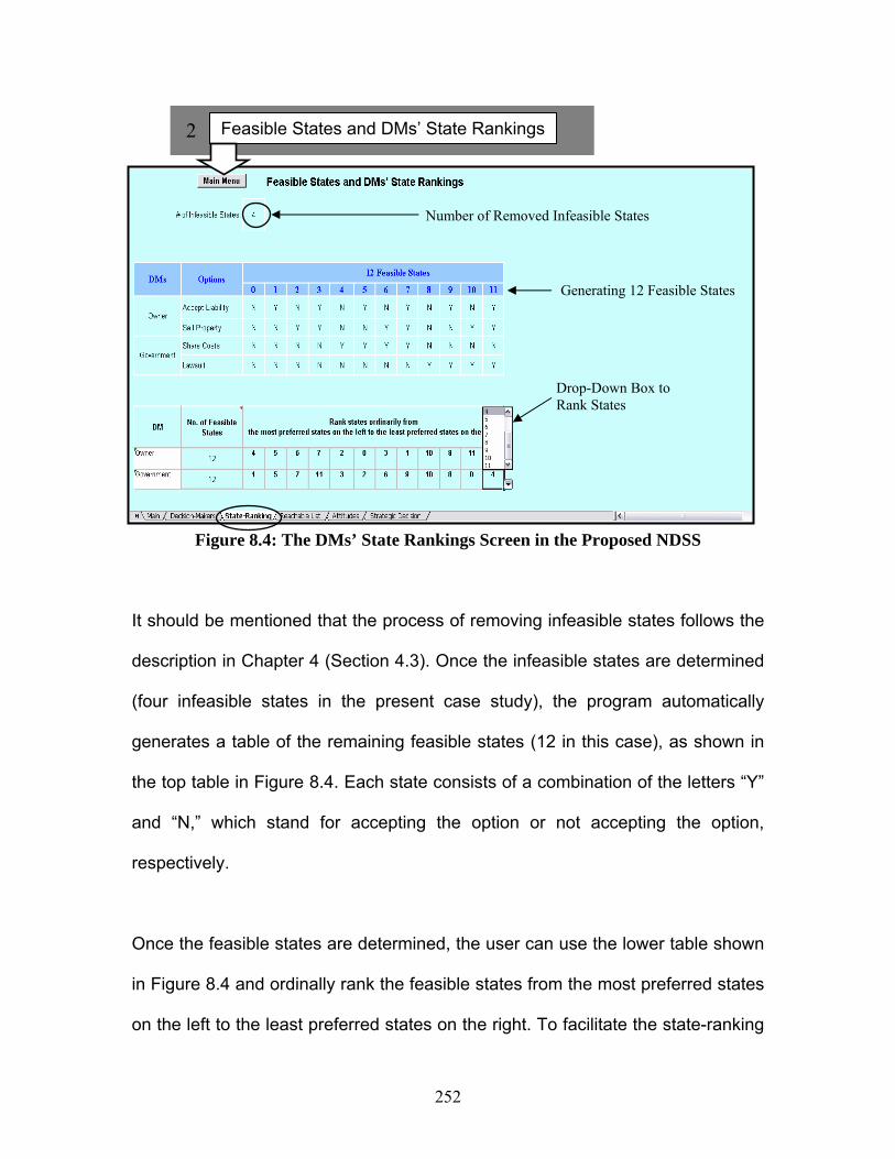
252
Figure 8.4: The DMs’ State Rankings Screen in the Proposed NDSS
It should be mentioned that the process of removing infeasible states follows the
description in Chapter 4 (Section 4.3). Once the infeasible states are determined
(four infeasible states in the present case study), the program automatically
generates a table of the remaining feasible states (12 in this case), as shown in
the top table in Figure 8.4. Each state consists of a combination of the letters “Y”
and “N,” which stand for accepting the option or not accepting the option,
respectively.
Once the feasible states are determined, the user can use the lower table shown
in Figure 8.4 and ordinally rank the feasible states from the most preferred states
on the left to the least preferred states on the right. To facilitate the state-ranking
Drop-Down Box to Rank States
Number of Removed Infeasible States
Generating 12 Feasible States
2 Feasible States and DMs’ State Rankings
253
process, the user can use the drop-down box in each cell to select an
appropriate feasible state. It should be mentioned that the program cannot
automatically rank the feasible states and that the user must rank the feasible
states with respect to each DM’s preference and considering all available
feasible states. The ordinal ranking of the feasible states is a necessary step in
the GMCR process.
8.3.3. Step 3: Specify the DMs’ Reachable Lists
In this step, the user specifies the DMs’ reachable lists (i.e., possible moves), as
shown in Figure 8.5. A reachable list is a record of all the feasible states that a
given DM can move to and from relative to the other feasible states. The DMs’
reachable list is used to determine which states represent an improvement for
each DM when their attitudes are incorporated into their decision to either move
to another state or remain in the current state.
The user first considers the state rankings of the DMs involved in this case study
negotiation. The drop-down box for each cell in the table allows the user to easily
find the available feasible states and select one appropriate state number for
each cell. As shown in Figure 8.5, the owner can move from state 8, for example,
to states 9, 10, or 11, and the government can move from state 8 to states 0 or 4,
as shown and indicated by two circles in the DMs’ state rankings in Figure 8.5. It
should be noted that according to a DMs’ moves, the DM shifts from one state to
another state, either better or worse.

254
Figure 8.5: Reachable Lists Screen in the Proposed NDSS
8.3.4. Step 4: Perform the Attitude-Based Stability Analysis
Once the DMs’ reachable lists are specified, the stability analysis, defined within
the paradigm of GMCR, is carried out. The attitude-based solution concepts (i.e.,
stability types), and the attitude-based definitions provided in Chapter 4 (Section
4.4) are implemented in a tableau that is used to model the moves and
countermoves of the DMs according to the attitudes of the DMs toward
The government can move from state 8 to states 0 or 4.
Drop-down box
3 DMs’ Reachable Lists
The owner can move from state 8 to states 9, 10 or 11.

255
themselves and one another. Figure 8.6 shows the DMs’ attitude matrix and the
stability analysis tableau for the present case study.
Figure 8.6: Automated Attitude-Based Stability Analysis Using the Proposed NDSS
As shown in Figure 8.6, the user should first enter an appropriate type for the
attitudes of the DMs toward themselves and one another using the attitude table
and the drop-down boxes provided for each cell. Three types of attitude are
defined in the boxes: positive, neutral, and negative. The user examines the
DMs’ attitudes according to the conflict situation and then enters the appropriate
4 Attitude-Based Stability Analysis
Equilibrium states, or possible conflict resolutions, depend on the DMs attitudes.

256
attitude term into each cell in the attitude table. Once the attitude terms have
been entered into the table, the program automatically carries out the stability
analysis in a systematic format within a tableau, as shown in Figure 8.6 and
according to the following sequential steps:
1. The program generates the DMs’ state rankings using the state-ranking
screen shown in Figure 8.4.
2. The program automatically determines the states underneath each state
in the DM’s state ranking using the DMs’ reachable lists discussed in
Subsection 8.3.3.
3. The program automatically determines the DMs’ moves from each state
in the DMs’ state rankings to the states within the DMs’ reachable lists,
using the DMs’ attitudes toward themselves and one another.
4. The program identifies the states within each DM’s state ranking from
which they have no move and marks them as NASH stable in the “DMs’
stability” row shown in the stability analysis tableau.
5. The program automatically analyzes the stability of the remaining states
involved in each DM’s state rankings, and determines the stability type of
the remaining states (e.g., RSEQ or U), according to the definition of
RSEQ and U provided in Section 4.4.
6. The program identifies the states within both DMs’ state rankings from
which they have at least one type of stability. If a state in both DMs’ state
rankings is marked with RNASH or RSEQ, then the program marks the
state as E in the “Equilibria (Final Results)” row shown in Figure 8.6.

257
As can be seen, the proposed prototype completely automates the attitude-
based stability analysis. The user needs to enter only the appropriate attitudes of
the DMs in the attitude table, and the program then quickly and accurately
provides the user with a possible equilibrium state. As discussed in Chapter 4, it
is very cumbersome to carry out an attitude-based stability analysis manually.
8.3.5. Step 5: Select a Strategic Decision
Once the attitude-based stability analysis has been carried out, the program
provides the user with a list of equilibrium states that are generated in table
format along with a description of each equilibrium state, as shown in Figure 8.7.
Figure 8.7: “Strategic Decision” Screen in the Proposed NDSS
5 Strategic Decision
After analyzing the three possible solutions, a final strategic decision is selected by the user.
258
Appropriate links have been defined between this worksheet and other
worksheets in this program. For example, the equilibrium state cells on the left
side of the table are linked to the cells in the equilibrium row shown in the stability
analysis tableau in Figure 8.6. The user reviews and analyzes the resulting
equilibrium states, or potential solutions for the conflict, and based on the current
conflict situation, selects the most beneficial solution at the strategic level.
As discussed in Chapter 4, the most beneficial strategic decision for the present
case study negotiation is equilibrium state 2, which was in fact agreed upon by
the DMs. As shown in Figure 8.7, a drop-down box is provided so that the user
can select the strategic decision; once the appropriate decision option is
selected, the description of the decision appears to the right of the state selected.
The state description helps the user identify the negotiation issues that will be
negotiated at the tactical level, as discussed in the following section.
8.4. Tactical Negotiation Support
The agreed-upon strategic decision can be further negotiated at the tactical level
in order to reach a mutual detailed resolution. The proposed NDSS includes a
tactical negotiation component which has been designed based on the tactical
negotiation methodology developed in Chapter 6. In the proposed methodology,
a polynomial utility function is assigned to each DM, and through interaction of
the DMs’ utility functions, an integrated utility function is obtained and used to
determine the settlement point, or the specific concession each DM should make

259
in order to reach a mutual detailed resolution. The tactical negotiation screen is
shown in Figure 8.8.
Figure 8.8: Tactical Negotiation Screen in the Proposed NDSS
The agreed-upon strategic decision selected for the present case study, as
shown in Figure 8.7, constitutes one issue for negotiation, which is the selling
price of the owner’s property. The DMs involved in the present case study
negotiation decide to cooperatively negotiate the issue and obtain the specific
concessions each DM should make in order to reach a mutual resolution at the
tactical level.
6 Tactical Negotiation
Attitude Table
))(100( 1)(
nnowner xU −=
nngovernment xU )100)(100( 1
)( −= −
260
Based on the above negotiation situation and the DMs’ positive attitude toward
themselves and each other, the user enters a positive attitude in the four cells in
the attitude table (Figure 8.8). Once the attitude table has been completed, the
program automatically adjusts an appropriate range for the n value, the power of
the polynomial utility function. Because the DMs have a positive attitude toward
each other in this situation, the program selects the range [1 < n ≤ 10], and the
user enters appropriate n values for the DMs, using the drop-down boxes shown
in Figure 8.8. Once the n values have been entered by the user, the program
automatically carries out the following sequential steps:
1. The program generates an appropriate number of rows (11 rows in
this case) for the middle table, as shown in Figure 8.8. The first
column on the left represents the x value of the DMs’ polynomial
utility functions and constitutes a 10% concession that each DM can
make in each step. The second, third, and fourth columns include
the numerical values for the utility functions of the owner, the
government, and the integrated function, respectively.
2. The program draws the DMs’ utility function form in a coordinated
system using the numerical values of the table generated in Step 1.
3. The program draws the integrated utility function form and specifies
the maximum point on it.
4. The program graphically reflects the maximum point of the
integrated utility function on the horizontal axis in order to show the
exact concession each DM should make, as circled in Figure 8.8.

261
As can be seen, the proposed prototype utilizes the concept of utility theory and
incorporates an easy-to-use graphical feature in order to determine the exact
concessions needed at the tactical level of negotiation. For example, Figure 8.8
depicts a situation in which the user selects the n values of 2 and 7 for the owner
and the government, respectively. The program then automatically carries out the
remaining tactical negotiation process and determines that a 30% concession
should be made by the government, and that a 70% (100% - 30%) concession
should be made by the owner with respect to the cost of the selling price of the
owner’s property. It should be noted that the DMs’ disagreement point, as
defined in Chapter 6, has not been considered in the proposed NDSS.
8.5. Summary
This chapter describes the implementation of the negotiation methodology
proposed in the previous chapters in a simplified negotiation decision support
system. The proposed prototype offers a promising framework for turning the
implicit experience gained by construction participants into the explicit expertise
needed for resolving the increasingly complex disputes that occur in the
construction industry. The design of the negotiation decision support system was
developed as a method of allowing the proposed negotiation methodology to be
conveniently applied to construction disputes. The scalability feature of the
proposed prototype allows future expansion, such as the consideration of the
weight and disagreement point for each issue and each DM, as well as the
262
consideration of multiple decision makers and multiple negotiation issues.
Moreover, sensitivity analysis at both the strategic and tactical levels of
negotiation can be considered using the proposed sensitivity analysis described
in the previous chapters.

263
CHAPTER 9: Conclusions 9.1. Introduction
This chapter presents a review of the contents of this thesis and provides a
summary of the conclusions and research contributions. It also highlights
recommendations and suggestions for future studies of the complex conflicts and
disputes that occur in the construction industry.
9.2. Research Summary
The goal of this research was to present a systematic, logically consistent, and
theoretically well-founded approach to the study of negotiation methodology for
resolving complex disputes in construction. Accordingly, a negotiation framework
was proposed in order to achieve the following objectives: 1) understand
construction negotiation and the attitudes of the decision makers; 2) develop a
negotiation methodology that considers the attitudes of the decision makers; and
3) design a negotiation decision support system.
To provide a good understanding of construction negotiation, a thorough analysis
of the characteristics of construction negotiations was performed, as provided in
Chapter 2, in order to identify the characteristics of negotiation, particularly those
related to the area of brownfield negotiations.

264
To develop a suitable negotiation methodology, two complementary levels of
negotiation have been considered, as described in Chapter 4: strategic and
tactical. With respect to the strategic level, the Graph Model for Conflict
Resolution (GMCR) was presented in Chapter 3. Chapter 4 described the
adaptation of GMCR to include consideration of the attitudes of the decision
makers with the goal of determining a potential strategic agreement that is the
most beneficial decision given the competing interests of the decision makers
involved. To that end, attitude was formally defined and represented within the
paradigm of GMCR. Attitude-based stability concepts, such as Nash stability and
Sequential stability were then defined, following which a variety of attitude
scenarios were examined and their results analyzed in order to determine the
most acceptable strategic decision.
The proposed negotiation methodology includes the in-depth tactical-level study
of the chosen strategic decision using attitude-based utility functions to help the
decision makers reach a mutually acceptable solution to the issues pending. As
described in Chapter 6, an attitude-based utility function is therefore defined for
each decision maker, according to the attitude of the decision maker. An
integrated utility function is then determined and used to identify the most
beneficial negotiated settlement with respect to each issue.
To demonstrate the advantages of the proposed negotiation methodology, two
construction case studies were used to explain the development of the proposed

265
methodology. The first case study, a brownfield negotiation between two decision
makers, was employed as presented and used in Chapters 4 and 6 in order to
illustrate the development of the negotiation methodology that considers the
attitudes of two decision makers. The second case study is a real-life brownfield
negotiation case involving multiple decision makers which is discussed in
Chapters 5 and 7 as a means of explaining the generalization of the negotiation
methodology for multiple decision makers. For this case study, six attitude
scenarios were identified and analyzed at the strategic level, as presented in
Chapter 5, in order to determine the sets of possible strategic decisions. These
sets were then analyzed and the most beneficial strategic decision selected. At
the tactical level for the second case study, a generalized methodology for
multiple decision makers was developed, as explained in Chapter 7, so that
pending issues can be resolved using two approaches: one issue at a time, and
two decision makers at a time. Using the latter approach, a mutual settlement for
each issue was suggested for the decision makers involved in the case study.
Chapter 7 also discusses the attitude-based sensitivity analysis which used the
Monte Carlo simulation to evaluate the sensitivity of the outcomes of the
negotiations to changes in the attitudes of the decision makers.
Once the negotiation methodology was developed and successfully applied to
the case studies, a simplified negotiation decision support system was designed,
as presented in Chapter 8. A prototype was developed that is capable of
266
handling and solving the challenging conflicts and the complex disputes that
occur in the construction industry.
The following are the main characteristics of the new negotiation methodology
that make it an efficient approach for resolving challenging construction conflicts
and disputes:
It systematically combines the strategic and tactical levels of decision
making and thereby offers complementary levels of decision making.
It formally defines attitude and models it within the proposed negotiation
methodology, thus providing a suitable approach for simulating the
behavior of decision makers.
It can consider multiple human factors, such as fear, anger, and hate, and
can define them within the structure of the proposed negotiation
framework.
It permits the use of a wide range of numerical scales that can describe
the quality of a solution at both levels.
It can be used for resolving complex construction disputes that involve
multiple decision makers and multiple conflicting issues.
It has been developed based on the characteristics of the construction
industry, such as its competitive-cooperative nature and its domain-
specific knowledge.
It takes into account the characteristics of construction negotiators, such
as their positions and choices.

267
It can be adapted to consider the characteristics of other types of disputes,
such as family disputes.
It employs the Graph Model technique by using attitude-based stability
concepts such as RNASH and RSEQ to study the negotiators’ actions and
counteractions during negotiations.
It consists of a supportive quantitative approach in addition to the
qualitative approach used in GMCR in order to determine the strategic
decision options.
It employs the concept of utility theory in order to help the decision makers
identify mutual agreement at the tactical level of negotiation.
It uses the proposed attitude-based utility functions to enable decision
makers to examine the impact of changes in their attitudes on the
outcomes of the tactical negotiations.
During the tactical negotiation process, it quantifies for each DM the
weight and disagreement point for each issue under negotiation.
It permits the decomposition of issues into sub-issues at the tactical level
of negotiation.
It incorporates a powerful sensitivity analysis to examine changes in the
negotiation outcomes at both the strategic and tactical levels of
negotiation.
It has been developed and successfully applied to brownfield negotiation
case studies involving multiple decision makers and multiple conflicting
issues.
268
9.3. Research Contributions
This research contributes significantly to the provision of managerial tools that
have the potential benefit of supporting construction negotiations by integrating
the strategic and tactical perspectives of negotiation while considering the
attitudes of the decision makers. The proposed attitude-based negotiation
introduces a new systems engineering methodology that will help managers
tackle a variety of real-world controversies, particularly in the construction
industry.
With respect to the strategic level of negotiation, the expansion of GMCR to
propose an attitude-based GMCR provides a flexible analytical tool that reflects
how the attitudes of the decision makers may change the outcome of the
negotiation. As well, the attitude-based solution concepts, defined within the
paradigm of GMCR, provide operational tools for assessing whether unwanted
consequences can result in a particular dispute because of improper attitudes.
With respect to the tactical level of negotiation methodology, the attitude-based
utility functions assist decision makers in ascertaining which attitudes are needed
in order to guide the conflict to more preferable, or win/win, solutions for all of the
decision makers concerned.
A negotiation decision support system is proposed in order to conveniently apply
the developed negotiation methodology to actual disputes. The proposed
negotiation decision support system has significant advantages with respect to

269
speed, accuracy, practicality, flexibility, reliability, and versatility. Moreover, the
proposed prototype offers a promising system for turning the implicit experience
gained by construction participants into the explicit expertise needed for resolving
the increasingly complex disputes that occur in the construction industry.
The research is expected to help improve negotiation methodologies for
resolving challenging construction disputes and thereby save significant amounts
of time and costs. The new methodology is also expected to help construction
decision makers both in the public and private sectors make more appropriate
decisions that will establish reliable engineering decision-making systems and
ensure the sustainable operation of constructed assets. The model developed in
this research is expected to provide the following important contributions:
1. The research is a step toward a better understanding of dispute resolution
and the negotiation process in the construction industry.
2. The developed model constitutes a more comprehensive negotiation
approach in which the strategic and tactical levels of negotiation are
complementarily combined.
3. The proposed negotiation methodology has a unique ability to take into
consideration the attitudes of the decision makers at both the strategic and
tactical levels of negotiation.
4. The proposed negotiation methodology has been conveniently implemented
into a simplified negotiation decision support system, which can provide

270
decision makers with significant advantages, such as automated negotiation
modeling, easy-to-use features, and more accurate results.
5. The developed methodology is expected to help in the re-engineering of
traditional construction negotiation processes. In other words, the useful
concepts presented in non-engineering sciences such as psychology and
sociology, can be used for developing negotiation support tools that provide
more beneficial outcomes.
6. The relationships among attitude-based stability concepts, such as RNASH
and RSEQ have been investigated, and relevant propositions have been
formally defined.
7. The attitude-based model proposed in this research provides a unique
opportunity to study the influence of other psychological factors, such as fear
and hate, on the outcomes of negotiation.
8. The research helps to foster a positive environment in which construction
professionals and practitioners can negotiate and therefore reduce the
destructive consequences of complicated disputes.
9. The research provides a major expansion of GMCR by combining attitudes
within the paradigm of GMCR which furnishes a flexible analytical tool which
reflects how the DMs’ attitudes may change the strategic negotiation
outcomes.
In addition to the above contributions, the research provides the decision makers
involved in brownfield disputes with an innovative negotiation framework that can

271
take into consideration the psychological factors involved in brownfield
negotiations. The proposed negotiation model may therefore assist participants
in brownfield disputes to resolve growing number of increasingly challenging
brownfield disputes around the globe in both developed and developing
countries. Finally, although the focus has been on negotiation support for
resolving construction disputes, the proposed system can be easily adapted to
other types of disputes, such as those related to families or other industries, such
as manufacturing or real estate.
9.4. Recommendations for Future Research
In spite of the inherent ability of the proposed negotiation framework to resolve
complex construction disputes, like many other methods of modeling negotiation,
it has limitations. A number of improvements which therefore would be beneficial
include the following suggestions for future research:
Study the cost of delays due to construction disputes, and consider the
effect of time and costs on the length of construction negotiation.
Conduct investigation that includes a variety of construction disputes, and
analyze practical approaches for resolving complex disputes.
Expand the three attitude types (i.e., positive, neutral, negative) to include
the wider range of attitude types that lie within the types defined for this
research.
Investigate the influence of other psychological factors (e.g., fear, hate,
and anger) on the outcomes of construction negotiations.

272
Consider the situation at the tactical level of negotiation in which all
decision makers intend to negotiate all conflicting issues simultaneously.
Study the interrelationships of the proposed attitude-based solution
concepts such as RNASH, RSMR, RGMR, and RSEQ.
Expand the design of the negotiation decision support system to consider
each DM’s disagreement point with respect to each negotiation issue.
Create an Internet (web-based) application from the current system to
enable multiple users to use and benefit from the system simultaneously.
Study the characteristics of negotiation and negotiators in other industries
and implement the developed negotiation model for resolving disputes in
other areas such as manufacturing, information technology, and
environmental management.
The results of conducting more comprehensive stability analyses would
undoubtedly lead to significant insight into the brownfield case studies and also
provide an enhanced methodology for incorporating the attitudes of the decision
makers into an interactive decision-making process.
It is believed that the model developed in this research will make the decision
process clear, transparent, and easy to track for all decision makers. In addition,
the decision makers involved in complex negotiations will be provided with more
sustainable solutions to their disputes. These advantages will likely help
construction participants make better decisions about resolving complex

273
disputes. Uninformed or faulty decision making can thus be significantly reduced,
thereby saving significant amounts of costs and resources, minimizing delays,
and maximizing cooperation and productivity in the construction industry.
274
References 1) Alfares, H.K., and Duffuaa, S.O. (2008). “Assigning cardinal weights in multi-
criteria decision making based on ordinal ranking”, Journal of Multi-Criteria Decision Analysis, John Wiley & Sons, Ltd. Publication, Published online in Wiley InterScience, (www.interscience.wiley.com) DOI: 10.1002/mcda.420, USA, pp. 1-9.
2) Aouad, G., Alshawi, M., and Bee, S. (1996). “Priority topics for construction information technology”, Int. Journal of Constr. Inf. Technol., Vol. 4, No. 2, pp. 45–66.
3) Aouad, G., and Price, A. (1994). “Construction planning and information technology in the UK and US construction industries: A comparative study”, Journal of Construction Management and Economic, Vol. 12, pp. 97–106.
4) Ash, S. (2004). New schools for Kitchener?, A report published in internet, <<http://72.14.205.104/search?q=cache:MjxsWt79atgJ:www.gvsa.on.ca/pharmacyschool.htm+Kitchener+LP+Holding&hl=en&ct=clnk&cd=1&gl=ca >>, Accessed on June 30, 2008.
5) Ausubel, L.M. (1991). “The failure of competition in the credit card market”, American Economic Review, Vol. 81, pp. 50-81.
6) Barnett, J. (1997). The Fractured Metropolis-improving the New City, Restoring the Old City, Reshaping the Region, New York: Harper Collins Publishing Inc., USA.
7) Barnett, R.S. (1997). “Alternate to dispute resolution: a growth industry”, Building Design and Constructions, Vol. 38, No. 3, pp. 44-48.
8) Bazerman, M.H. (1994). Judgment in Managerial Decision Making, John Wiley & Sons, New York, USA.
9) Bell, D.E., Raiffa, H., and Tversky, A. (1988). Decision making: descriptive, normative, prescriptive interactions, Cambridge University Press, New York, NY 10013-2473, USA.
10) Bellucci, E. and Zeleznikow, J. (1998). “A comparative study of negotiation decision support systems”, Thirty-First Annual Hawaii International Conference on System Sciences, Vol. 1, pp. 254.
11) Begley, R. (1997). “Resurrecting brownfields”, Environmental Science and Technology, Vol. 31, No. 5, pp. 226A– 230A.
12) Bellucci, E., and Zeleznikow, J. (1998). “Family_negotiator: an intelligent decision support system for negotiation in Australian family law”, The Fourth Conference of the International Society of Decision Support Systems, Lausanne, Switzerland, pp. 359 – 374.
13) Belton. V., and Stewart, T.J. (2001). Multiple criteria decision analysis: an integrated approach. Kluwer Academic Publishing: Emeryville, CA 94608, USA.
14) Benazon, N. (1995). “Soil remediation: a practical overview of Canadian cCleanup strategies and commercially available technology”, Hazardous Materials Management (Fall), pp. 10-26.

275
15) Bennett, pp. (1998). “Confrontation analysis as a diagnostic tool,” European Journal of Operational Research, Vol. 109, pp. 465-482.
16) Bennett, pp., and Howard, N. (1996). ”Rationality, emotion and preference change- drama theoretic model of choice,” European Journal of Operational Research, Vol. 92, pp. 603-614.
17) Bichler, M., Kersten, G., and Weinhardt, C. (2003). “Electronic negotiations: foundations, systems, and experiments - introduction to the special issue”, Group Decision and Negotiation, Vol. 12, pp. 85-88.
18) Bourne, L.S. (1995). “Reurbanization and urban land development: US cities in comparative context”, Washington: Office of Technology Assessment, Congress of the United States.
19) Brams, S.J., and Kilgour, D.M. (2001). “Fallback bargaining”, Group Decision and Negotiation, Vol. 10, pp. 287-316.
20) Brooker, pp., and Lavers, A. (1997). “Perceptions of alternate dispute resolution as constraints upon use in the U.K construction industry”, Construction Management and Economics, Vol. 15, No. 6, pp. 519-526.
21) Bryant, J. (2003). The six dilemmas of collaboration: Inter-organizational relationships as drama, Wiley, Chichester, UK.
22) Buccola, S.T. (1982). “Portfolio selection under exponential and quadratic utility”, Western Journal of Agricultural Economics, Vol. 7, pp. 43-51.
23) Camerer, C.F. (1995). Individual decision making, In J.H. Kagel & A.E. Roth (Eds.), Handbook of Experimental Economics, Princeton, NJ: Princeton University Press, USA, pp. 587-703.
24) Cheung, S., and Suen, H.C.H. (2002). “A multi-attribute utility model for dispute resolution strategy selection”, Construction Management and Economics, No. 20, pp. 557–568.
25) Cheung, S., Suen, H.C.H., and Lam, T.I. (2002), “Fundamentals of alternative dispute resolution processes in construction”, Journal of Construction Engineering and Management, Vol. 128, No. 5, pp. 409-417.
26) Cheung, S., Yiu, K.T.W., and Suen, H. (2004), “Construction negotiation online”, Journal of Construction Engineering and Management, Vol. 130, Issue 6, pp. 844-852.
27) Cheung, S.O., Yiu, T.W.Y., and Yeung, S.F. (2006). “A Study of styles and outcomes in construction dispute negotiation”, Journal of Construction Engineering and Management, Vol. 132, No. 8, pp. 805-905.
28) Chubb, J. (2006). Exploring links between negotiating styles and assertiveness building, www.younevercantell.co.uk, Accessed on June, 02, 2007.
29) Churchman, D. (1993). “Negotiation tactics”, University Press of America Inc., 4720 Boston Way, Lanham, Maryland, USA.
30) Cohen, S. (2002). Negotiating skills for managers, New York: McGraw-Hill. 31) Colosi, T. (1999). A core model of negotiation, In Negotiation, R. J. Lewicki,
D. M. Saunders, & J. M. Minton (Eds.), New York: IrwinIMcGraw Hill, USA, pp. 313-319.
32) Darling, T., and Mumpower, J.L. (1990). "Modeling cognitive influences on the dynamics of negotiations", Proceedings of the 23rd Annul International

276
Conference on Systems Sciences, IEEE Computer Society Press, pp. 22–30.
33) Department of Justice Canada (1995). Dispute resolution in Canada: a survey of activities and services, report # TR1995-1e.
34) De Sousa, C.A. (2000), The brownfield problem in urban Canada: issues, approaches, and solutions, PhD dissertation, Graduate Department of Geography, The University of Toronto. Ontario, Canada.
35) De Sousa, C. (2001). “Contaminated sites: the Canadian situation in an international context”, Journal of Environmental Management, Vol. 62, pp. 131–154.
36) Di-Donato, L. (1993). “Alternative methods to resolve contract disputes: approaches to effective prevention”, American Association of Cost Engineers, Transaction of the American Association of Cost Engineers, Morgantown, W.Va, USA.
37) Diekmann J.E., and Girard, M.J. (1995). “Are contract disputes predictable?”, Journal of Construction Engineering and Management., Vol. 121, No. 4, pp. 355- 363.
38) Doug, J. (2006). “Construction project dispute resolution: options for effective dispute avoidance and management”, Journal of Professional Issues in Engineering Education and Practice, Forum in July, pp. 225-236.
39) Du, T.C., and Chen, H.L. (2007). “Building a multiple-criteria negotiation support system”, IEEE transactions on knowledge and data engineering, Vol. 19, No. 6, pp. 804 – 817.
40) Dudziak, W., and Hendrickson, C. (1988). “Simulation game for contract negotiations”, Journal of Management in Engineering, Vol. 4, No. 2, pp. 113-121.
41) Dunlop, J.T. (1984), “Dispute resolution; negotiation and consensus building”, Auburn House Publishing Company, Dover, Massachusetts, USA, pp. 6-10.
42) Eliashberg, J., and Winkler, R.L. (1978). “The role of attitude toward risk in strictly competitive decision-making situations”, Journal of Management Science, Vol., 24, No. 12, pp. 1231 – 1241.
43) Ellerbusch, F. (2006). “Brownfields: risk, property, and community value”, Journal of Local Environment, Vol. 11, No. 5, pp. 559–575.
44) Encyclopedia of Life Support Systems (EOLSS), (2002), Eolss Publishers, Oxford, UK, accessed from http://www.eolss.co.uk, and http://www.eolss.com.
45) Essex, R.J. (1996). “Means of avoiding and resolving disputes during construction”, Tunneling and Underground Space Technology, Vol. 11, No. 1, pp. 27-31.
46) Fang, L., Hipel, K.W., and Kilgour, D.M. (1993). Interactive Decision Making: The Graph Model for Conflict Resolution, New York: Wiley, USA.
47) Fang, L., Hipel, K.W., Kilgour, D.M., and Peng, X. (2003a). “A decision support system for interactive decision making, part 1: model formulation”, IEEE Transactions on Systems, Man, and Cybernetics, Part C, Vol. 33, No. 1, pp. 42-55.
277
48) Fang, L., Hipel, K.W., Kilgour, D.M., and Peng, X. (2003b). “A decision support system for interactive decision making, part 2: analysis and output interpretation”, IEEE Transactions on Systems, Man, and Cybernetics, Part C, Vol. 33, No. 1, pp. 56-66.
49) Fearon, J.D. (1995). "rationalist explanations for war", International Organization, Vol. 49, No. 3, pp. 379-414.
50) Fellow, R.F., Seymour, D., and Hankock, M.R. (1994). “Conflict resulting from cultural differentiation: an investigation of the new engineering contract”, pp. Fenn (Ed.), Construction Conflict: Management and resolution. CIB Publication 171, CIB, The Netherlands, pp. 259-268.
51) Fenn, pp., Lowe, D., and Speck, C. (1997). ”Conflict and dispute in construction”, Construction Management and Economics, No.15, Issue 6, pp. 513 - 518.
52) Fishburn, pp. C. (1970). Utility theory for decision making. Huntington, NY. Robert E. Krieger Publishing Co. 1970. ISBN 978-0471260608.
53) Fisher, R., Ury, W., and Patton, B. (1991). Getting to yes: negotiating agreement without giving in (2nd Edition). New York: Penguin, USA.
54) Fraser, N.M., and Hipel, K.W. (1984). Conflict analysis: models and resolutions, New York: North Holland.
55) Garrett, D. (2002). “The owners perspective in construction management”, Construction Management and Economics, Vol. 15, No. 7, pp. 87-96.
56) Gibson, G.E., and Gebken II, R.J. (2006). Decision making, transactional costs and dispute resolution: is there a better way?, Department of Civil, Architectural, and Environmental Engineering, University of Texas at Austin, USA.
57) Gillie, pp., Goetz, pp., Muller, F., and Feinberg, K.R. (1991). Using mediation to resolve construction disputes’’, Alternative dispute resolution in the construction industry, R. F. Cushman, G. C. Hedemann, and A. S. Tucker, eds., Wiley Law, New York, pp. 153–210.
58) Glasner, K. (2000). “Contract disputes, the role of ADR”, Dispute Resolution Journal, Vol. 55, No. 3, pp. 50-55.
59) Halter, A.N., and Dean, G.W. (1971). Decision under uncertainty with research applications, South-Western Publishing, Cincinnati, OH, USA.
60) Hammond, J.S., Keeney, R.L., and Raiffa, H. (1999). Smart choices: a practical guide to making better decisions, Harvard Business School Press, Boston, Massachusetts, USA.
61) Hamouda, L., Kilgour, D., and Hipel, K. (2004). “Strength of preferences in the graph model for conflict resolution”, Group Decision and Negotiation, Vol. 13, pp. 449-462.
62) Hanoch, G., and Levy, H. (1981). “Efficient portfolio selection with quadratic and cubic utility”, Journal of Business, No. 43, pp. 181-189.
63) Harmon, K.M.J. (2003). ”Resolution of construction disputes: a review of current methodologies”, Leadership Management Engineering, Vol. 3, No. 4, pp. 187-201.

278
64) Hartman, F.T., and Jergeas, G.F. (1995). “A model for proactive mediation of construction disputes”, Canadian Journal of Civil Engineering, Vol. 22, pp. 15-22.
65) Hegazy, T., and Ayed, A. (1998). “Neural network model for parametric cost estimation of highway pProjects”, Journal of Construction Engineering and Management, Vol. 24, No.3, pp. 210-218.
66) Hegazy, T., and Ayed, A. (1999). “Simplified spreadsheet solutions: models for CPM and TCT analyses”, Cost Engineering, AACE International, AACE, Vol. 41, No.7, pp.26-33.
67) Hegazy, T. (2002). Computer-based construction project management., Prentice Hall, Upper saddle River. USA. pp. 11 – 38.
68) Hegazy, T., Elhakeem, A., and Elbeltagi, E. (2004). “Distributed scheduling model for infrastructure networks”, Journal of Construction Engineering and Management, ACSE, Vol.130, pp.160-167.
69) Hegazy, T. (2006). “Advanced project management” Course Notes, Department of Civil Engineering, University of Waterloo, Ontario, Canada.
70) Henderson, D.A. (1996). “Mediation success: an empirical analysis”, Ohio St. Journal On Dispute Resolution, pp. 105.
71) Heng, L. (1996). “Case-based reasoning for intelligent support of construction negotiation”, Journal of Information and Management, Vol. 30, No. 5, pp. 231-238.
72) Hipel, K.W. (2003). “Conflict resolution”, theme overview paper, Conflict resolution, Encyclopaedia of Life Support Systems (EOLSS), Eolss Publishers, Oxford, UK, accessed from http://www.eolss.net.
73) Hipel, K.W. (2005). Conflict resolution, the course notes of the courses SYDE 533 and SYDE 730, Department of Systems Design Engineering, University of Waterloo, Waterloo, Ontario, Canada.
74) Hipel, K.W. (Editor) (2008a). Conflict resolution, Vol. 1, Eolss Publisher, Oxford, United Kingdom.
75) Hipel, K.W. (Editor) (2008b). Conflict resolution, Vol. 2, Eolss Publisher, Oxford, United Kingdom.
76) Hipel, K.W., and Ben-Haim, Y. (1999). “Decision making in an uncertain world: information-gap modelling in water resources management”, IEEE Transaction on system, Man, and Cybernetics, Vol. 29, No. 4, pp. 506-517.
77) Hipel, K.W., and Fang, L., (2005). "Multiple participant decision making in societal and technological systems", in Arai, T., Yamamoto, S. and Makino, K. (Editors), Systems and Human Science – For Safety, Security, and Dependability: Selected Papers of the 1st International Symposium, SSR2003, Osaka, Japan, published by Elsevier, Amsterdam, The Netherlands, Chapter 1, pp. 3-31.
78) Hipel, K.W., Hegazy, T., and Yousefi, S. (2009). “Combined strategic and tactical negotiation methodology for resolving complex brownfield conflicts”, Unpublished Manuscript, Department of Systems Design Engineering, University of Waterloo, Waterloo, Ontario, Canada, 2009.

279
79) Hipel, K.W., Jamshidi, M.M., Tien, J.M., and White, C.C. (2007). “The future of systems, man, and cybernetics: application domains and research methods”, IEEE Transactions on Systems, Man, and Cybernetics-Part C: Applications and Reviews, Vol. 37, No. 5, pp. 726 – 743.
80) Hipel, K.W., Kilgour, D.M., Fang, L., and Peng, J. (1997). “The decision support system GMCR in environmental conflict management”, Applied Mathematics and Computation, Vol. 83, No’s. 2 and 3, pp. 117-152.
81) Hipel, K.W., Kilgour, D.M., and Rajabi, S. (1999). Operations research and refinement of courses of action, Handbook of systems engineering and management, A.pp. Sage and W.B. Rouse (Editors), Wiley, New York, pp. 1077– 1118.
82) Honeyman, C., Goh, B.C., and Kelly, L. (2004). “Skill is not enough: seeking connectedness and aAuthority in mediation”, Negotiation Journal, Vol. 20, Issue 4, pp. 489.
83) Howard, R.A. (1971). “Proximal decision analysis”, Journal of Management Science, Vol. 17, pp. 507-541.
84) Howard, N. (1971). Paradoxes of rationality: theory of metagames and political behavior, Cambridge, Massachusetts: MIT Press, USA.
85) Howard, N. (1990). “’Soft’ game theory”, Information and Decision Technologies, Vol. 16, No. 3, pp. 215-227.
86) Howard, N. (1994). “Drama theory and its relation to game theory, Part 1: dramatic resolution vs. rational choice”, Group Decision and Negotiation, Vol. 3, pp. 187-206.
87) Howard, N. (1994). “Drama theory and its relation to game theory, Part 2: formal model of the resolution process”, Group Decision and Negotiation, Vol. 3, pp. 207-235.
88) Howard, N. (1998). “n-person ‘soft’ games”, Journal of Operational Research Society, Vol. 49, pp. 144-150.
89) Howard, N. (1999). Confrontation analysis: How to win operations other than war, CCRP Publications, Pentagon, Washington, DC, USA.
90) Hsee, C.K., and Kunreuther, H. (2000). “The affection effect in insurance decisions”, Journal of Risk and Uncertainty, Vol. 20, pp. 141–59.
91) Inohara, T., Hipel, K.W., and Walker, S. (2007). “Conflict analysis approaches for investigating attitudes and misperceptions in the war of 1812”, Journal of Systems Science and Systems Engineering, Vol. 16, No. 2, pp. 1-21.
92) Inohara, T., and Hipel, K.W. (2008a). “Coalition analysis in the graph model for conflict resolution”, Journal of Systems Engineering, Vol. 11, No. 4, pp. 343-359.
93) Inohara, T., and Hipel, K.W. (2008b). “Interrelationships among Noncooperative and Coalition Stability Concepts”, Journal of Systems Science and Systems Engineering, Vol. 17, No. 1, pp. 1-29.
94) Inohara, T., Yousefi, S., and Hipel, K.W. (2008). “Propositions on interrelationships among attitude-based stability concepts”, invited paper published in the special session on Conflict and Risk Analsyis in Systems Management in the Proceedings of the 2008 IEEE International
280
Conference on Systems, Man, and Cybernetics, held in the Suntec Singapore International Convention and Exhibition Centre, Singapore, October 12-15, 2008, pp.2502-2507.
95) Isen, A.M., and Geva, N. (1987). “The influence of positive affect on acceptable level of risk: the person with a large canoe has a large worry”, Organizational Behavior and Human Decision Process, Vol. 39, pp.145-154.
96) Jarke, M., Jellasi, M.T., and Shakun, M.F. (1987). “MEDIATOR: towards a negotiation support system”, European Journal of Operational Research, Vol. 31, No. 3, pp. 314-334.
97) Jergeas, G.F. (2008). “Analysis of the front-end loading of Alberta mega oil sands projects”, Project Management Journal, Vol. 39, No. 4, pp. 95-104.
98) Ji, S., Liang, Y., Xiao, X., Li, J., and Tian, Q. (2007). “An attitude-adaptation negotiation strategy in electronic market environments”, Eight ACIS International Conference on Software Engineering, Artificial Intelligence, Networking, and Parallel/ Distributed Computing, IEEE Computer Sociaety, pp. 125-130.
99) Johnson, E.J., and Tversky, A. (1983). “Affect, generalization, and the perception of risk”, Journal of Personality and Social Psychology, Vol. 45, pp. 20–31.
100) Kagel, J.H., and Roth, A.E. (1995). Handbook of experimental economics, Princeton, NJ: Princeton University Press, USA.
101) Kahneman, D., and Tversky, A. (1979). “Prospect theory: an analysis of decision under risk”, Econometrica, Vol. 47, pp. 263-291.
102) Kahneman, D., and Tversky, A. (2000). Choices, values, and frames, Cambridge: Cambridge University Press, USA.
103) Kassab, M., Hipel, K.W., and Hegazy, T. (2006). “Conflict resolution in construction disputes using the graph model”, Journal of Construction Engineering and Management, Vol.132, No.10, pp. 1043-1052.
104) Keeney, R.L., (1992). Value-focused thinking, Harvard University Press, Cambridge, Massachusetts, USA.
105) Keeney, R.L., and Raiffa, H. (1976). Decisions with multiple objectives: Preferences and value tradeoffs, New York: Wiley, USA.
106) Kellogg, J.C. (2001). ‘‘The contract disputes resolution continuum’’, Kellogg News, Vol. 11, No. 1, pp. 2.
107) Kersten, G.E. (2001). “Modeling distributive and integrative negotiations. review and revised characterization”, Group Decision and Negotiation, Vol. 10, No. 6, pp. 493-514.
108) Kersten, G.E. (2002). “The science and engineering of e-negotiation: an introduction”, Proceedings of the 36th Hawaii International Conference on System Sciences (HICSS’03), hicss, vol. 1, pp. 27a.
109) Kersten, G.E. (2005). “E-negotiation systems: interaction of people and technologies to resolve conflict”, The Magnus Journal of Management, Vol. 11, No. 3, pp. 71-96.
281
110) Kilgour, D.M., Hipel, K.W., Fang, L., and Peng X. (2001). “Coalition analysis in group decision support”, Group Decision and Negotiation, Vol. 10, No. 2, pp.159-175.
111) Kilgour, D.M. (2006). Introduction to game theory, Mathematics (MA 235) Course Package, Wilfrid Laurier University Press, Waterloo, Ontario, Canada.
112) Kilgour, D.M. (2007). Diplomacy game: the graph model for conflict resolution as a tool for negotiators, Springer Berlin, Heidelberg, Part IV, pp. 251 - 263.
113) Kirkwood, C.W. (1997). Notes on attitude towards risk taking and exponential utility function, Department of Management, Arizona State University, Tempe, AZ, USA.
114) Krech, D., Crutchfield, R. S., and Ballachey, E. L. (1962). Individual in society: a textbook of social psychology, McGraw-Hill, New York, USA.
115) Kumaraswamy, M. (1997). “Conflict, claims and disputes in construction”, Engineering and Architectural Management, Vol. 4, No.1, pp. 95–111.
116) Lax, D., and Sebenius, J. (1992). The manager as negotiator: the negotiator's dilemma: creating and claiming value in dispute resolution, 2nd ed., edited by Goldberg, Frank Sander and Nancy Rogers, Boston: Little Brown and Co., pp. 49-62.
117) Levin, pp. (1998). Construction contract claims, changes, and dispute resolution, ASCE Press, 1801 Alexander Bell Drive Reston, VA 20191-4400, pp. 6 – 21.
118) Li, H. (1996). “Case-based reasoning for intelligent support of construction negotiation”, Journal of Information and Management, Vol. 30, Issue 5, pp. 231-238.
119) Li, K., Kilgour, D.M., and Hipel, K.W. (2004). “Status quo analysis of the Flathead river conflict”, Water Resources Research, Vol. 40, pp. 1-9.
120) Li, K., Hipel, K.W., and Kilgour, D.M. (2004). “Integrating uncertain preferences into status quo analysis: an environmental conflict case study”, IEEE international Conference on Systems, Man and Cybernetics, pp. 1092-1097.
121) Lin, W., Dean, G.W., and Moore, C.V. (1974). “An empirical test of utility vs. profit maximization in agricultural production”, American Journal of Agriculture and Economy, Vol. 56, pp. 497-508.
122) Lin, W., and Chang, H.S. (1978). “Specification of bernoullian utility functions in decision analysis”, American Journal of Agriculture and Economy, Vol. 30, pp. 30-36.
123) Loosemore, M. (1999). “Bargaining tactics in construction disputes”, Construction Management and Economics, No.17, pp.177- 188.
124) Lootsma, F.A. (1999). “Multi-criteria decision analysis via ratio and difference judgment”. Kluwer Academic Publishers, Emeryville, CA 94608, USA.
125) LTSF, Litigation Trends Survey Findings (2006). The third annual report of the LTSF, Fulbright and Jaworski L.L.pp., Available on: www.fulbright.com, accessed on June 05, 2007, pp. 11-12.

282
126) Lukas, J.A, and Lukas, J.L. (2008). “Project negotiations: deal yourself a winning hand”, the proceedings for the Project Management Institute (PMI) Global Congress, North America, Oct. 14 – 16, Denver, Colorado, USA.
127) Mathews, A.A. (1997).”The first dispute review board”, Foundation Forum, Vol. 1, No. 1.
128) Matwin, S., Szpakowicz, S., Koperczak, Z., Kersten, G.E., and Michalowski, W. (1989). “Negoplan: an expert system shell for negotiation support”, IEEE Intelligent Systems, Vol. 4, No. 4, pp. 50-62.
129) Mbabazi, A., Hegazy, T., and Saccomanno, Frank. (2005). “Modified but-for method for delay analysis”, Journal of Construction Engineering and Management, ACSE, Vol.131, pp. 1142-1144.
130) Mix, D. (1997). “ADR in the construction industry: continuing the development of a more efficient dispute resolution mechanism”, 12 Ohio State Journal On Dispute Resolution, pp. 463.
131) Mnookin, R., Peppet, S.R., and Tulumello, A.S. (2000). Beyond winning: negotiating to create value in deals and disputes, The Belnap Press of Harvard University Press, USA.
132) Molenaar, K., Washington, S., and Diekmann, J. (2000). “Structural equation model of construction contract dispute potential”, Journal of Construction Engineering and Management., Vol. 126, Issue 4, pp. 268-277.
133) Morley, I.E. (1981). Bargaining and negotiation, in psychology and management, Cooper, C.L. (ed), Macmillan, London, pp. 95 - 127.
134) Morris, pp. (1994). Introduction to game theory, Springer-Verlag Publishing, New York, USA.
135) Mumpower, J.L. (1991). “The judgment policies of negotiators and the structure of negotiation problems”, Journal of Management Science, Vol. 37, No. 10, pp. 1304-1324.
136) Mumpower, J.L. (1988). "An analysis of the judgmental components of negotiation and a proposed judgmentally-oriented approach to mediation", In B. Brehmer and C.R.B. foyce (eds.), human judgment: The SIT approach, Amsterdam: North Holland, pp. 465-502.
137) Musser, W.N., Wetzstein, M.E., Reece, S.Y., Musser, L.M., Varca, pp.E., and Chou, C.C.J. (1984). “Classification of risk preferences with elicited utility data: Does the functional form matter?”, Agricultural Economics Journal, Vol. 9, pp. 322-328.
138) Muthoo, A. (1999). Bargaining theory with applications, Cambridge, Cambridge University Press, USA.
139) Myerson, R.B. (1991). Analysis of incentives in bargaining and mediation, negotiation analysis, H. pp. Young. Ann Arbor, University of Michigan Press, pp. 67-85.
140) Nash, J.F. (1950). “Equilibrium points in n-person games”, Proceedings of National Academy of Sciences, Vol. 36, pp. 48-49.
141) Nash, J.F. (1951). “Noncooperative games”, Annals of Mathematics, Vol. 54, No. 2, pp. 286-295.
283
142) Ngee, L., Tiong, R.L.K., and Alum, J. (1997). “Automated approach to negotiation of BOT contracts”, Journal of Computing in Civil Engineering, Vol. 11, Issue 2, pp. 121-128.
143) O’Brien, M., and Al-Soufi, A. (1994). “A survey of data communications in the UK construction industry”, Journal of Construction Management and Economy, Vol. 12, pp. 457– 465.
144) Ock, J.H., and Han, S.H. (2003). “Lessons learned from rigid conflict resolution in an organization: construction conflict case study”, Journal of Management in Engineering, Vol. 19, No. 2, pp. 83 – 89.
145) Odeh, A.M., and Battaineh, H.T. (2002). “Causes of construction delay: traditional contracts”, International Journal of project Management, Vol. 20, No. 1, pp. 67-73.
146) Office of Government Commerce, OGC, (2002). Dispute resolution Guidance, Office of Government Commerce, Rosebery Court, St Andrews Business Park, Norwich, the UK., pp. 4.
147) Omoto, T., Kobayashi, K., and Onishi, M. (2002). “Bargaining model of construction dispute resolution”, Systems, Man and Cybernetics, 2002 IEEE International Conference, Vol. 7, pp. 6-17.
148) Pena-Mora, F., and Wang, C.Y. (1998). “Computer-supported collaborative negotiation methodology”, Journal of Computing in Civil Engineering, Vol. 12, No. 2, pp. 64 – 81.
149) Pinnell, S. (1999). ‘‘Partnering and the management of construction disputes’’, Dispute Resolution Journal, Vol. 54, No. 1, pp. 16–22.
150) Prelec, D. (2000). Compound invariant weighting functions in prospect theory. In Kahneman & Tversky (Eds.), Choices, Values, and Frames. Cambridge: Cambridge, University Press.
151) Rabin, M. (1998). “Psychology and economics”, Journal of Economic Literature, Vol. XXXVI, pp. 11-46.
152) Raiffa, H., Richardson, J., and Metcalfe, D. (2002). Negotiation analysis: the science and art of collaborative decision making. Cambridge: The Belknap Press of Harvard University Press, USA.
153) Rameezdeen, R., and Gunarathna, N. (2003). “Disputes and construction industry cultures”, AACE International Transactions, ABI/INFORM Global, pp. CD 241-248.
154) Ren, Z., Anumba, C.J., and Ugwu, O.O. (2003). “Negotiation in a multi-agent system for construction claims negotiation”, Applied Artificial Intelligence, Vol. 16, pp. 359-394.
155) Richter, I.E. (2000). "The project neutral: neutralizing risk, maintaining relationships and watching the bottom line", Construction Business Review, Vol. 8, No. 2, pp. 52-54.
156) Rottenstreich, Y., and Hsee, C.K. (2001). “Money, kisses, and electric shocks: on the affective psychology of risk”, Psychological Science, Vol. 12, pp.185–190.
157) Saaty, T.L. (1980). The analytic hierarchy process, McGraw-Hill, New York, NY, USA.

284
158) Saaty, T.L. (1990). Multi-criteria decision making: the analytic hierarchy process, RWS Publications, Pittsburgh, PA. USA.
159) Saaty, T.L. (1994). Fundamentals of decision making and priority theory with the analytic hierarchy process, RWS Publications, Pittsburgh, PA, USA.
160) Sage, A.pp., and Rouse, W.B. (1999). Handbook of systems engineering and management, Wiley, New York, USA.
161) Savage, L.J. (1971). “Elicitation of personal probabilities and expectations”, Journal of. American Statistic Association, Vol. 66, pp. 783-801.
162) Scott, B., and Billing, B. (1990). Negotiating skills in engineering and construction, Thomas Telford Publication, London, the UK, pp. 71 – 83.
163) Sebenius, J.K. (1992). "Negotiation analysis: a characterization and review", Management Science, Vol. 38, No. 1, pp. 18-38.
164) Semple, C., Hartman, F., and Jergeas, G. (1994). “Construction claims and disputes: causes and cost/time overruns”, Journal of Construction Engineering and Management ASCE, Vol. 120, No. 4, pp. 785-794.
165) Shash, A.A., and Al-Amir, M. (1997). “Information technology in contractors’ firms in Saudi Arabia”, Construction Management and Economy, Vol. 15, pp. 187– 200.
166) Shen, L.Y., Bao, H.J., Wu, Y.Z., and Lu, W.S. (2007). “Using bargaining-game theory for negotiating concession period for BOT-type contract”, Journal of Construction Engineering and Management, Vol. 133, No. 5, pp. 385 – 392.
167) Shin, K.C. (2000). Identification of critical dispute characteristics during construction project operations, PhD dissertation, Georgia Institute of Technology, United States of America.
168) Smith, M.L. (1992). “Planning your negotiation”, Journal of Management in Engineering, Vol. 8, No. 3, pp. 254-260.
169) Stipanowich, T.J. (1997). “At the cutting edge: conflict avoidance and resolution in the US construction industry”, Journal of Construction Management & Economics, Vol. 15, pp. 505- 512.
170) Sycara, K. (1993). “Negotiation planning, an AI approach”, European Journal of operations Research, Issue. 46, pp. 216-234.
171) Thaler, R.H. (1988). “The ultimatum game”, Journal of Economic Perspectives, Vol. 2, No. 4, pp. 195- 206.
172) Thiessen, E.M., and McMahon, J.pp. (2000). “Beyond win-win in cyberspace”, Ohio State Journal on Dispute Resolution, Issue 15, pp. 643.
173) Trantina, T.L. (2001). ‘‘An attorney’s guide to alternative dispute resolution (ADR): ‘ADR 1.01’’, Presented at the New Jersey Bar Association, Justice Marie L. Garibaldi America Inn of Court for Alternative Dispute Resolution, N.J., USA.
174) Treacy, T.B. (1995). “Use of alternative dispute resolution in the construction industry”, Journal of Management in Engineering, Vol. 11, No. 1, pp. 58-63.
285
175) Tversky, A., and Kahneman, D. (1991). “Loss aversion in riskless choice: a reference dependent model”, Quarterly Journal of Economics, pp.1039-1061.
176) Tversky, A., and Kahneman, D. (1986). “Rational choice and the framing of decisions”, Journal of Business, Vol. 59, No. 4, pt.2, pp. 251-278.
177) Tyler, T.R. (2000). “Social justice: outcome and procedure”, International Journal of Psychology, Vol. 35, pp. 117-125.
178) Von Neumann, J., and Morgenstern, O. (1953). Theory of games and economic behaviour, 3 rd. Princeton University Press, USA.
179) Von Neumann, J., and Morgenstern, O. (1944). Theory of games and economic behaviour, 1st. New York Wiley, USA.
180) Von Winterfeld, D., and Edwards, W. (1986). Decision analysis and behavioural research, Cambridge: Cambridge University Press.
181) Walton, R.E., Cutcher-Gershenfeld, J.E., and McKersie, R.B. (2000), Strategic negotiations, ILR Press and imprint of Cornell University Press, pp. 223 – 257.
182) Wertheim, E., Love, A., Littlefield, L., and Peck, C. (1992). I win: you win Penguin Books, Ringwood, Victoria, Australia, pp. 130-135.
183) Yaoyueyong, C., Hadikusumo, B.H.W., Ogunlana, S.O., and Siengthai, S. (2005). “Virtual construction negotiation game – an interactive learning tool for project management negotiation skill training”, International Journal of Business & Management Education, Vol. 13, No. 2, pp. 21 – 37.
184) Young, H.pp. (1991). Negotiation analysis, Negotiation Analysis. H. pp. Young. Ann Arbor, University of Michigan Press, pp. 1-23.
185) Yousefi, S., Hegazy, T., and Hipel, K.W. (2009). “Managing construction conflicts using attitude-based negotiation.”, Proceedings of the 2nd International/8th Construction Specialty Conference, Canadian Society for Civil Engineering (CSCE), Annual General Meeting and Conference, held in St. John’s, Newfoundland and Labrador, Canada, May 27-30, 2009.
186) Yousefi, S., Hegazy, T., and Hipel, K.W. (2009). Attitude-based negotiation for resolving complex disputes in construction projects. An invited presentation to the First Canadian Graduate Student Curriculum on Computer-Assisted Construction Technology, held in the Construction Centre, National Research Council Canada, London, Ontario. Canada, June 18 –19, 2009.
187) Yousefi, S., Hipel, K.W., and Hegazy, T. (2009). Extended abstract, “Attitude-based negotiation for resolving brownfield disputes”. Proceedings of the International Conference on Group Decision and Negotiation (GDN), Westin Harbour Castle, Toronto, Ontario, Canada, June 14 – 17, pp. 189 - 192.
188) Yousefi, S., Hipel, K.W., and Hegazy, T. (2008). "An attitude-based negotiation methodology for the management of construction disputes," Accepted for publication on the American Society for Civil Engineering (ASCE) Journal of Management in Engineering. Accepted for Publication on March 20, 2009.

286
189) Yousefi, S., Hipel, K.W., and Hegazy, T. (2008). "Construction negotiations: does attitude matter?" Proceedings of the Canadian Society for Civil Engineering (CSCE), Annual General Meeting and Conference, held in the Quebec City Convention Centre, Quebec City, Quebec, Canada, June 10-13, pp. 289-297.
190) Yousefi, S., Hipel, K.W., and Hegazy, T. (2008). "Psychological aspects of construction negotiations." An invited Presentation to the 8th Graduate Studies Research Conference, held in David Centre (DC), University of Waterloo, Waterloo, Ontario, Canada.
191) Yousefi, S., Hegazy, T., Attalla, M., and Capuruco, R.A.C. (2008). “System of multiple ANNs for online planning of numerous building improvements”, Journal of Construction Engineering and Management, Vol. 134, No. 5, pp. 342-351.
192) Yousefi, S., Hipel, K.W., Hegazy, T., Witmer, J.A., and Gray, P. (2007). “Negotiation characteristics in brownfield redevelopment projects”, invited paper published in the special session on Conflict and Risk Analysis in Systems Management in the Proceedings of the 2007 IEEE International Conference on Systems, Man, and Cybernetics, held in The Delta Centre-Ville, Montreal, Quebec, Canada, October 7-10, pp 1866-1871.
193) Yousefi, S., Hipel, K.W., Hegazy, T., Witmer, J.A., and Gray, P. (2007). Extended Abstract, ”Cooperative brownfield redevelopment for an educational institution”, Proceedings of Group Decision and Negotiation, the 4th Annual International Conference on Group Decision and Negotiation, May 14 – 17, 2007, Montreal, Quebec, Canada.
194) Yuan, Y., Suarga, R.B., and Archer, N. (1998). "A web-based negotiation support system", International Journal of Electronic Markets, Vol. 8, No. 3, pp. 13-17.
195) Zack, J.G. (1995). “Practical dispute management”, Cost Engineering, Vol. 37, No. 12, pp. 55-63.
196) Zeleznikow, J., Bellucci, E., Schild, U.J., and MacKenzie, G. (2007). “Bargaining in the shadow of the law - using utility functions to support legal negotiation”, Proceedings of the International Conference on Artificial Intelligence and Law, Eleventh International Conference on Artificial Intelligence and Law, pp. 237-246.
197) Zeleznikow, J. (2002). “Risk, negotiation and argumentation; a decision support system-based approach”, Journal of Law Probability and Risk, Vol.1, No. 1, pp. 37-48.
198) Zhang, X., Lesser, V., and Podorozhny, R. (2005). “Multi-dimensional, multi-step negotiation”, Journal of Autonomous Agents and Multi-Agent Systems, Vol. 10, No. 1, pp. 5-40.
199) Zuhair, S.M.M., Taylor, D.B., and Kramer, R.A. (1992). “Choice of utility function form: its effect on classification of risk preferences and the prediction of farmer decisions”, Journal of Agricultural Economics, Vol. 6, pp. 333-344.

287
APPENDIX A Computer Program for Removing Infeasible Attitude Cases It should be noted that the results of the following programming codes, written in java, are summarized in Tables 5.6, 5.7, and 5.8, presented in Chapter 5. ******************************************************************************************* // Computer Program for Generating Various Attitude Cases and // Removing Infeasible Attitude Cases import java.util.Scanner; import java.io.*; public class AttitudeGenerator1 { //instance variables private int numOfDemakers; private int numofAttudes; private int[][] attitudeArray; private int arrayDimention; public AttitudeGenerator1(int howManyDm, int howManyAtts)//Constructor { numOfDemakers=howManyDm; numofAttudes=howManyAtts; arrayDimention=((int)Math.pow(howManyAtts, howManyDm*howManyDm)); attitudeArray= new int[arrayDimention][howManyDm*howManyDm+1]; int [] attitudeType= new int [3]; attitudeType[0]=+1; //positive attitude attitudeType[1]= 0; //neutral attitude attitudeType[2]=-1; //negative attitude int index=-1; int count=1; for (int ii=0; ii<numOfDemakers*numOfDemakers; ii++) //initialize attitudeArray { count=numofAttudes*count; int position=arrayDimention/count; for (int i=0; i<arrayDimention; i++) { if (i % position ==0) { index++; }

288
attitudeArray[i][ii]=attitudeType[index]; if ((index+1)==3 && ((i+1)%position==0) ) { index=-1; } } } } public void printAttitudeArray( int perLinePrint)// print attitudeArray in a text file named attitude.txt { PrintWriter outputStream =null; try { outputStream = new PrintWriter(new FileOutputStream("attitude.txt")); } catch(FileNotFoundException e) { System.out.println("Error opening the file attitude.txt."); System.exit(0); } int rpt=this.arrayDimention/perLinePrint; for (int iii=0; iii<rpt; iii++) { int ctr=0; for (int i=0; i<this.numOfDemakers;i++) { int temp=i*this.numOfDemakers; for (int j=iii*perLinePrint; j<iii*perLinePrint+perLinePrint; j++) { ctr=temp; for (int ii=0; ii<this.numOfDemakers;ii++) { outputStream.print(this.attitudeArray[j][ctr]); int repeat=CalSpace(this.attitudeArray[j][ctr], 3); for (int k=0; k<repeat; k++) { outputStream.print(" "); } ctr++; if ((ii+1) % this.numOfDemakers ==0 ) { outputStream.print("|"); }
289
} } outputStream.println(); } for (int i=0; i<(this.numOfDemakers*3+1)*perLinePrint; i++) { outputStream.print("-"); } outputStream.println(); } int ctr=0; for (int i=0; i<this.numOfDemakers;i++) { int temp=i*this.numOfDemakers; for (int j=rpt*perLinePrint; j<this.arrayDimention; j++) { ctr=temp; for (int ii=0; ii<this.numOfDemakers;ii++) { outputStream.print(this.attitudeArray[j][ctr]); int repeat=CalSpace(this.attitudeArray[j][ctr], 3); for (int k=0; k<repeat; k++) { outputStream.print(" "); } ctr++; if ((ii+1) % this.numOfDemakers ==0 ) { outputStream.print("|"); } } } outputStream.println(); } outputStream.close(); } public void printInLine() //print attitudeArray in a line-base in a text file named attitudePrintedInLine.txt { PrintWriter outputStream =null;; try { outputStream = new PrintWriter(new FileOutputStream("attitudePrintedInLine.txt")); }

290
catch(FileNotFoundException e) { System.out.println("Error opening the file attitudePrintedInLine.txt."); System.exit(0); } for (int i=0; i<this.arrayDimention;i++) { for (int j=0; j<(numOfDemakers*numOfDemakers); j++) { if (j % numOfDemakers==0 && j!=0 ) { outputStream.print(" | "); } int rpt=CalSpace(attitudeArray[i][j],3); for (int ii=0; ii<rpt; ii++) { outputStream.print(" "); } outputStream.print(attitudeArray[i][j]); } outputStream.println(); } outputStream.close(); } private static int CalSpace(int var, int base)//number of spaces needed to be left while printing { int space=base-Integer.toString(var).length(); return space; } public void CalculationOfInfeasibilities() // recording infeasible cases in a text file named infeasibles.txt { PrintWriter outputStream =null; try { outputStream = new PrintWriter(new FileOutputStream("infeasibles.txt")); } catch(FileNotFoundException e) { System.out.println("Error opening the file infeasibles.txt."); System.exit(0); } int [] position=new int [this.numOfDemakers]; int pos=0;
291
for (int i=0; i<this.numOfDemakers; i++) { position[i]=pos; pos=pos+this.numOfDemakers+1; } int counter12=0; int counter13=0; int counter23=0; int counter123=0; int counter1=0; int counter2=0; int counter3=0; int Counter1=0; int Counter2=0; int Counter12=0; int [][] temp1=new int [this.arrayDimention/this.numofAttudes][4]; int [][] temp2=new int [this.arrayDimention/this.numofAttudes][4]; int [][] temp3=new int [this.arrayDimention/this.numofAttudes][4]; for (int i=0; i<this.arrayDimention; i++) { if (this.numOfDemakers==2) { if (this.attitudeArray[i][position[0]]==-1 && this.attitudeArray[i][position[1]]!=-1 ) { for (int ii=0; ii<4;ii++) { temp1[Counter1][ii]=this.attitudeArray[i][ii]; } Counter1++; } if (this.attitudeArray[i][position[1]]==-1 && this.attitudeArray[i][position[0]]!=-1 ) { for (int ii=0; ii<4;ii++) { temp2[Counter2][ii]=this.attitudeArray[i][ii]; } Counter2++; } if (this.attitudeArray[i][position[1]]==-1 && this.attitudeArray[i][position[0]]==-1 ) { for ( int ii=0; ii<4; ii++) { temp3[Counter12][ii]=this.attitudeArray[i][ii];

292
} Counter12++; } } if (this.numOfDemakers==3) { if (this.attitudeArray[i][position[0]]==-1 && this.attitudeArray[i][position[1]]!=-1 && this.attitudeArray[i][position[2]]!=-1 ) { counter1++; } if (this.attitudeArray[i][position[1]]==-1 && this.attitudeArray[i][position[0]]!=-1 && this.attitudeArray[i][position[2]]!=-1 ) { counter2++; } if (this.attitudeArray[i][position[2]]==-1 && this.attitudeArray[i][position[1]]!=-1 && this.attitudeArray[i][position[0]]!=-1 ) { counter3++; } if (this.attitudeArray[i][position[0]]==-1 && this.attitudeArray[i][position[1]]==-1 && this.attitudeArray[i][position[2]]!=-1 ) { counter12++; } if (this.attitudeArray[i][position[0]]==-1 && this.attitudeArray[i][position[2]]==-1 && this.attitudeArray[i][position[1]]!=-1 ) { counter13++; } if (this.attitudeArray[i][position[1]]==-1 && this.attitudeArray[i][position[2]]==-1 && this.attitudeArray[i][position[0]]!=-1 ) { counter23++; } if (this.attitudeArray[i][position[0]]==-1 && this.attitudeArray[i][position[1]]==-1 && this.attitudeArray[i][position[2]]==-1 ) { counter123++; } } } if (this.numOfDemakers==2)

293
{ outputStream.println("DM1 negative and DM2 only neural and positive ==> "+Counter1+" Infeasible Cases "); int perLinePrint=10; int rpt=Counter1/perLinePrint; for (int iii=0; iii<rpt; iii++) { int ctr=0; for (int i=0; i<this.numOfDemakers;i++) { int temp=i*this.numOfDemakers; for (int j=iii*perLinePrint; j<iii*perLinePrint+perLinePrint; j++) { ctr=temp; for (int ii=0; ii<this.numOfDemakers;ii++) { outputStream.print(temp1[j][ctr]); int repeat=CalSpace(temp1[j][ctr], 3); for (int k=0; k<repeat; k++) { outputStream.print(" "); } ctr++; if ((ii+1) % this.numOfDemakers ==0 ) { outputStream.print("|"); } } } outputStream.println(); } for (int i=0; i<(this.numOfDemakers*3+1)*perLinePrint; i++) { outputStream.print("-"); } outputStream.println(); } int ctr=0; for (int i=0; i<this.numOfDemakers;i++) { int temp=i*this.numOfDemakers; for (int j=rpt*perLinePrint; j<Counter1; j++) { ctr=temp; for (int ii=0; ii<this.numOfDemakers;ii++) {
294
outputStream.print(temp1[j][ctr]); int repeat=CalSpace(temp1[j][ctr], 3); for (int k=0; k<repeat; k++) { outputStream.print(" "); } ctr++; if ((ii+1) % this.numOfDemakers ==0 ) { outputStream.print("|"); } } } outputStream.println(); } outputStream.println(); outputStream.println("DM2 negative and DM1 only neural and positive ==> "+Counter2+" Infeasible Cases "); int rpt1=Counter1/perLinePrint; for (int iii=0; iii<rpt1; iii++) { int ctr1=0; for (int i=0; i<this.numOfDemakers;i++) { int temp=i*this.numOfDemakers; for (int j=iii*perLinePrint; j<iii*perLinePrint+perLinePrint; j++) { ctr1=temp; for (int ii=0; ii<this.numOfDemakers;ii++) { outputStream.print(temp2[j][ctr1]); int repeat=CalSpace(temp2[j][ctr1], 3); for (int k=0; k<repeat; k++) { outputStream.print(" "); } ctr1++; if ((ii+1) % this.numOfDemakers ==0 ) { outputStream.print("|"); } } } outputStream.println(); } for (int i=0; i<(this.numOfDemakers*3+1)*perLinePrint; i++)
295
{ outputStream.print("-"); } outputStream.println(); } int ctr2=0; for (int i=0; i<this.numOfDemakers;i++) { int temp=i*this.numOfDemakers; for (int j=rpt*perLinePrint; j<Counter2; j++) { ctr2=temp; for (int ii=0; ii<this.numOfDemakers;ii++) { outputStream.print(temp2[j][ctr2]); int repeat=CalSpace(temp2[j][ctr2], 3); for (int k=0; k<repeat; k++) { outputStream.print(" "); } ctr2++; if ((ii+1) % this.numOfDemakers ==0 ) { outputStream.print("|"); } } } outputStream.println(); } outputStream.println(); outputStream.println("DM1 and DM2 simultaneously negative ==> "+Counter12+" Infeasible Cases "); int rpt3=Counter12/perLinePrint; for (int iii=0; iii<rpt3; iii++) { int ctr3=0; for (int i=0; i<this.numOfDemakers;i++) { int temp=i*this.numOfDemakers; for (int j=iii*perLinePrint; j<iii*perLinePrint+perLinePrint; j++) { ctr3=temp; for (int ii=0; ii<this.numOfDemakers;ii++) { outputStream.print(temp3[j][ctr3]); int repeat=CalSpace(temp3[j][ctr3], 3);

296
for (int k=0; k<repeat; k++) { outputStream.print(" "); } ctr3++; if ((ii+1) % this.numOfDemakers ==0 ) { outputStream.print("|"); } } } outputStream.println(); } for (int i=0; i<(this.numOfDemakers*3+1)*perLinePrint; i++) { outputStream.print("-"); } outputStream.println(); } int ctr4=0; for (int i=0; i<this.numOfDemakers;i++) { int temp=i*this.numOfDemakers; for (int j=rpt3*perLinePrint; j<Counter12; j++) { ctr4=temp; for (int ii=0; ii<this.numOfDemakers;ii++) { outputStream.print(temp3[j][ctr4]); int repeat=CalSpace(temp3[j][ctr4], 3); for (int k=0; k<repeat; k++) { outputStream.print(" "); } ctr4++; if ((ii+1) % this.numOfDemakers ==0 ) { outputStream.print("|"); } } } outputStream.println(); } outputStream.close(); } if (this.numOfDemakers==3)
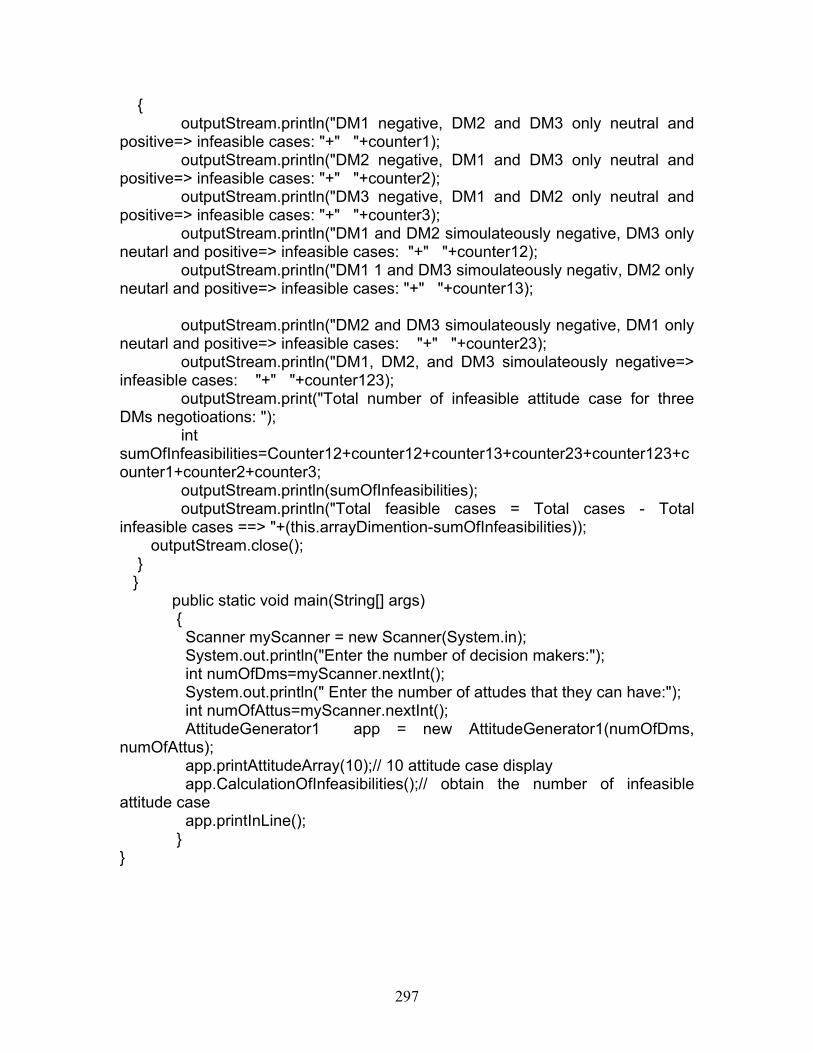
297
{ outputStream.println("DM1 negative, DM2 and DM3 only neutral and positive=> infeasible cases: "+" "+counter1); outputStream.println("DM2 negative, DM1 and DM3 only neutral and positive=> infeasible cases: "+" "+counter2); outputStream.println("DM3 negative, DM1 and DM2 only neutral and positive=> infeasible cases: "+" "+counter3); outputStream.println("DM1 and DM2 simoulateously negative, DM3 only neutarl and positive=> infeasible cases: "+" "+counter12); outputStream.println("DM1 1 and DM3 simoulateously negativ, DM2 only neutarl and positive=> infeasible cases: "+" "+counter13); outputStream.println("DM2 and DM3 simoulateously negative, DM1 only neutarl and positive=> infeasible cases: "+" "+counter23); outputStream.println("DM1, DM2, and DM3 simoulateously negative=> infeasible cases: "+" "+counter123); outputStream.print("Total number of infeasible attitude case for three DMs negotioations: "); int sumOfInfeasibilities=Counter12+counter12+counter13+counter23+counter123+counter1+counter2+counter3; outputStream.println(sumOfInfeasibilities); outputStream.println("Total feasible cases = Total cases - Total infeasible cases ==> "+(this.arrayDimention-sumOfInfeasibilities)); outputStream.close(); } } public static void main(String[] args) { Scanner myScanner = new Scanner(System.in); System.out.println("Enter the number of decision makers:"); int numOfDms=myScanner.nextInt(); System.out.println(" Enter the number of attudes that they can have:"); int numOfAttus=myScanner.nextInt(); AttitudeGenerator1 app = new AttitudeGenerator1(numOfDms, numOfAttus); app.printAttitudeArray(10);// 10 attitude case display app.CalculationOfInfeasibilities();// obtain the number of infeasible attitude case app.printInLine(); } }
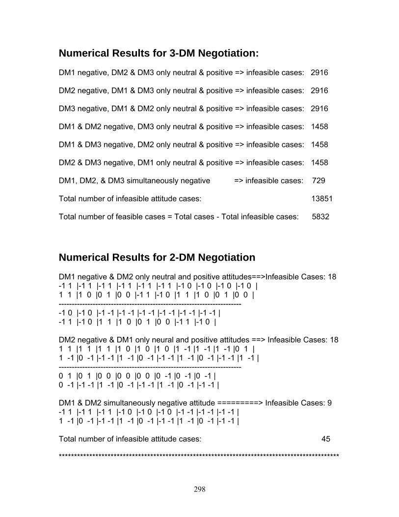
298
Numerical Results for 3-DM Negotiation: DM1 negative, DM2 & DM3 only neutral & positive => infeasible cases: 2916 DM2 negative, DM1 & DM3 only neutral & positive => infeasible cases: 2916 DM3 negative, DM1 & DM2 only neutral & positive => infeasible cases: 2916 DM1 & DM2 negative, DM3 only neutral & positive => infeasible cases: 1458 DM1 & DM3 negative, DM2 only neutral & positive => infeasible cases: 1458 DM2 & DM3 negative, DM1 only neutral & positive => infeasible cases: 1458 DM1, DM2, & DM3 simultaneously negative => infeasible cases: 729 Total number of infeasible attitude cases: 13851 Total number of feasible cases = Total cases - Total infeasible cases: 5832 Numerical Results for 2-DM Negotiation DM1 negative & DM2 only neutral and positive attitudes==>Infeasible Cases: 18 -1 1 |-1 1 |-1 1 |-1 1 |-1 1 |-1 1 |-1 0 |-1 0 |-1 0 |-1 0 | 1 1 |1 0 |0 1 |0 0 |-1 1 |-1 0 |1 1 |1 0 |0 1 |0 0 | ---------------------------------------------------------------------- -1 0 |-1 0 |-1 -1 |-1 -1 |-1 -1 |-1 -1 |-1 -1 |-1 -1 | -1 1 |-1 0 |1 1 |1 0 |0 1 |0 0 |-1 1 |-1 0 | DM2 negative & DM1 only neural and positive attitudes ==> Infeasible Cases: 18 1 1 |1 1 |1 1 |1 0 |1 0 |1 0 |1 -1 |1 -1 |1 -1 |0 1 | 1 -1 |0 -1 |-1 -1 |1 -1 |0 -1 |-1 -1 |1 -1 |0 -1 |-1 -1 |1 -1 | ---------------------------------------------------------------------- 0 1 |0 1 |0 0 |0 0 |0 0 |0 -1 |0 -1 |0 -1 | 0 -1 |-1 -1 |1 -1 |0 -1 |-1 -1 |1 -1 |0 -1 |-1 -1 | DM1 & DM2 simultaneously negative attitude =========> Infeasible Cases: 9 -1 1 |-1 1 |-1 1 |-1 0 |-1 0 |-1 0 |-1 -1 |-1 -1 |-1 -1 | 1 -1 |0 -1 |-1 -1 |1 -1 |0 -1 |-1 -1 |1 -1 |0 -1 |-1 -1 | Total number of infeasible attitude cases: 45 ********************************************************************************************