ATOMIC SPECTROSCOPY: Introduction to the Theory of Hyperfine Structure

ATOMIC SPECTROSCOPY: Introduction to the Theory of Hyperfine Structure

ANATOLI ANDREEV M.V. Lomonosov Moscow State University Moscow. Russia

Springer -

Anatoli V. Andreev M.V. Lomonosov Moscow State University

Atomic Spectroscopy: lntroduction to the Theory of Hypefine Structure

Consulting Editor: D. R. Vij

lSBN 10 0-387-25.573-7 e-ISBN 0-387-28469-9 Printed on acid-free paper. ISBN 13 9780387255736

O 2006 Springer Science+Business Media, lnc. All rights reserved. This work may not be translated or copied in whole or in part without the written permmion of the publisher (Springer Science+Business Media, Inc., 233 Spring Street, New York, NY 10013, USA), except for brief excerpts in connection with reviews or scholarly analysis. Use in connection with any form of information storage and retrieval, electronic adaptation, computer software, or by similar or dissimilar methodology now known or hereafter developed is forbidden. The use in this publication of trade names, trademarks, service marks and similar terms, even if they are not identified as such, is not to be taken as an expression of opinion as to whether or not they are subject to proprietary rights.

Printed in the United States of America.

9 8 7 6 5 4 3 2 1 SPIN L 1054344

Contents

Preface Acknowledgments

1. INTRODUCTION

1.1 Experiments with single particle in Penning trap

1.2 Spectroscopy of hydrogenlike atoms

1.3 Experiments on search for electric dipole moment of elementary particles and atoms

Part I Fine and Hyperfine Structure of Atomic Spectra

2. SCHRODINGER EQUATION

Schrodinger equation 2.1.1 Schrodinger and Heisenberg equations 2.1.2 Continuity equation, boundary conditions, and

normalization condition 2.1.3 Gauge transformation

Quantum mechanical operators 2.2.1 Momentum operator 2.2.2 Space inversion and parity operator 2.2.3 Three-dimensional rotations and

momentum operator

Particle motion in the Coulomb field 2.3.1 Discrete spectrum 2.3.2 Continuous spectrum 2.3.3 Matrix elements of transitions

Hydrogen atom 2.4.1 Hamiltonian of two-particle problem

angular

xi xiii

1

2

4

7

13

13 13

16 18

19 20 21

22

24 25 3 1 3 1

34 34

ATOMIC SPECTROSCOPY

2.4.2 Reduced electron mass 2.4.3 Atom in trap 2.4.4 Interaction of trapped atom with electromagnetic

field

3. VARIATIONAL PRINCIPLE FOR SCHRODINGER EQUATION: ORBITAL INTERACTION IN HYDROGENLIKE ATOMS

3.1 Particle wave fields 3.1.1 Lagrange function 3.1.2 Hamiltonian function 3.1.3 Action for particle interacting with electromagnetic

field

3.2 Symmetry properties with respect to orthogonal transformations 3.2.1 Orthogonal transformations 3.2.2 Space inversion 3.2.3 Spatial translation 3.2.4 Three-dimensional rotations 3.2.5 Transformations including time axis

3.3 Many-electron atom 3.3.1 Action principle for many-electron atom 3.3.2 Hydrogen atom 3.3.3 Integrals of motion 3.3.4 Energy level shift due to orbital interaction in

hydrogenlike atoms

4. PAUL1 EQUATION

4.1 Spin 4.1.1 Spin operator 4.1.2 Pauli matrix and spinors 4.1.3 Hamiltonian of Pauli equation

4.2 Geonium atom 4.2.1 Electron motion in homogeneous magnetic field 4.2.2 Strength of induced magnetic field

4.3 Hydrogen atom 4.3.1 Action for ensemble of non-relativistic spin-112

particles 4.3.2 Orbital, spin-orbital, and spin-spin interactions 4.3.3 Integrals of motion for hydrogen atom

Contents vii

4.3.4 Angular dependency of hydrogenic wave functions 90 4.3.5 Angular matrix elements of Hamiltonian of spin-

orbital and spin-spin interactions 94 4.3.6 Equations for radial wave functions 9 7 4.3.7 Influence of orbital, spin-orbital, and spin-spin

interactions on the energy spectrum of hydrogen atom 99

5. RELATIVISTIC EQUATION FOR SPIN ZERO PARTICLE 105

5.1 Klein-Gordon-Fock equation 105

5.2 Interaction of zero spin particle with electromagnetic field 107

5.3 Mesoatom 5.4 Wave functions

6. DIRAC EQUATION

6.1 Dirac matrices

6.2 Covariant form of the Dirac equation

6.3 Symmetry properties of the Dirac equation with respect to the orthogonal transformations 6.3.1 Three-dimensional rotations 6.3.2 Lorentz transformation 6.3.3 Space inversion 6.3.4 Time reversal 6.3.5 Charge conjugation 6.3.6 C PT invariance

6.4 Free particle 6.4.1 Planewaves 6.4.2 Helicity 6.4.3 Particleand antiparticle 6.4.4 Spherical waves

6.5 Particle interaction with electromagnetic field 136 6.5.1 Pauli equation 138 6.5.2 Non-relativistic approximation 139 6.5.3 Motion in Coulomb field 141

viii ATOMIC SPECTROSCOPY

Part I1 Theory of Lamb Shift

7. THEORY OF SPIN-112 PARTICLES INTERACTING WITH ELECTROMAGNETIC FIELD

7.1 Action principle 7.2 Connections with the Dirac equation

7.3 Symmetry properties with respect to orthogonal transformations 7.3.1 Space inversion 7.3.2 Three-dimensional rotations 7.3.3 Lorentz transformation 7.3.4 Time reversal 7.3.5 Charge conjugation 7.3.6 CPT invariance

7.4 Wave function normalization condition 7.5 Plane waves

7.5.1 Particle-antiparticle transformation 7.5.2 Space inversion, three-dimensional rotation,

Lorentz transformation, and time reversal 7.5.3 Charge conjugation

7.6 Spherical waves 7.61 Spherical spinors 7.6.2 Plane wave expansion in spherical harmonics

series 7.6.3 Convergent and divergent spherical waves

8. PARTICLE MOTION IN STATIC EXTERNAL FIELDS 8.1 Integrals of motion

8.1.1 Free particle 8.1.2 Particle motion in centro-symmetric fields 8.1.3 Cylindrically symmetric external fields

8.2 Electron motion in Coulomb field 8.2.1 General solution 8.2.2 Discrete spectrum 8.2.3 Continuous spectrum

8.3 Geonium atom 8.3.1 Electron motion in homogeneous magnetic field 8.3.2 Energy spectrum 8.3.3 Induced magnetic field

Contents ix

8.4 Neutron motion in static magnetic field 8.4.1 Neutron reflection by magnetic field 8.4.2 Neutron scattering by localized magnetic field 8.4.3 The bound states of neutron in magnetic field

9. ORIGIN OF LAMB SHIFT

9.1 Static fields

9.2 Symmetric form of the filed equations

9.3 Lamb shift

9.4 Neutron interaction with the static electric field 9.4.1 Neutron reflection by the static electric field 9.4.2 Symmetry properties of wave function 9.4.3 Reflection and transmission coefficients 9.4.4 Electric and magnetic polarization vectors of

neutron scattered by electric field 9.4.5 Bound states of neutron and antineutron in

the electric field

9.5 Neutron motion in superposition of electric and magnetic fields 9.5.1 Parallel fields 9.5.2 Crossed fields

9.6 Geonium atom 9.7 Hyperfine structure of hydrogenic spectra: comparison

with the experimental data

10. HYDROGEN ATOM

10.1 Action principle

10.2 Steady-state case

10.3 Integrals of motion 10.4 Angular dependency of hydrogen atom wave functions

10.5 Equations for radial wave functions

10.6 Perturbation theory

10.7 The case of j = 0

10.8 Internal parity

References

Index

Preface

There are a lot of excellent books on atomic spectroscopy today, but, hopefully, the distinctive feature of this book is its generality. We are not involved in the discussion of some specific mechanisms of formation of complex structure of atomic spectra, we are not trying to give an overview of different methods and models that are uscd to describe the spectra and to get a reasonable coincidence of calculated and measured data. We have tried to discuss comprehensively the general approach to the theory of atomic spectra, based on the use of the Lagrangian canonical formalism. The Lagrangian formalism enables us to easily generalize any Hamiltonian for electron motion in the external field to the Hamiltonian of many-electron problem, as a result the specific and common features of these two problems become more evident. The non-relativistic or relativistic, spin or spinless particle approximations can be used as a starting point in the general approach. All these approximations are analyzed and compared. This generality is helpf~~l to keep the important points from technicalities of spccific theories. The specific examples, that are used to illustrate the general approach, are chosen from contemporary atomic spectroscopy and light-matter inter- action physics (trapped atom, mesoatom, high-precision measurements of electron anomalous magnetic moment and hydrogenic spectra, electric polarization vector of nucleons, etc.).

The book consists of two main parts. The first part deals with the hyperfine structure associated with the finite mass of nucleus, its orbital motion, and spin-spin interaction. The second part of the book deals mainly with the Lamb shift. The specific feature is that the theory of Lamb shift is based on the use of quantum mechanics. The obtained equation for hydrogenic spectrum has a very simple and compact form, as a result the physics of Lamb shift formation can be easily interpreted.

xii Preface

Notice, that usually the students of atomic spectroscopy theory are not deeply familiar with the methods of quantum electrodynamics the- ory, which is traditionally used to explain the physics of Lamb shift. Therefore the proposed approach makes the theory accessible for a wide range of specialists and students, who are familiar with the quantum mechanics and classical electrodynamics.

The basic equations and principles of quantum mechanics are briefly discussed in the book, therefore it can be used as a self-consistent textbook providing enough material for half-year or one-year course for graduate students: "Introduction into atomic spectroscopy1', "Hyperfine structure of atomic spectra", etc.

Acknowledgments

I gratefully acknowledge the support of Physics Department, M.V. Lo- monosov Moscow State University, in whose stimulating environment I have been working for more than twenty five years. My personal thanks to my colleagues from International Laser Center, M.V. Lomonosov Moscow State University, the interaction with them for many years and numerous discussions are a great source of inspiration in my researches. The main ideas of this book have been discussed in a number of con- ferences, symposiums, and scientific seminars. I am grateful to those who asked me the tricky questions. Especially, I would like to thank the participants of the scientific seminars headed by Prof. E.B. Alek- sandrov (A.I. Ioffe Physical Technical Institute, St.Petersburg), Prof. L.V. Keldysh (P.N.Lebedev Physical Insitute, Moscow), Prof. V.A. Ma- karov (Physics Department, M.V. Lomonosov Moscow State University), Prof. M.O. Scully (TAMU, College Station, Texas). I would like to thank Prof. Olga Kocharovskaya and Prof. Vitali Kocharovskiy for hos- pitality during my stay at Texas A&M University, where the significant part of the book was prepared. Thanks are also due to Ilya Shutov and Eugeny Morozov, who helped me to prepare U w files until I learned how to do it.

Finally, very special thanks to my wife Mary and to my daughters Olga and Tatiana, who contributed with their support and patience during this long work.

The most part of the original results, which, I think, are the very important for the content of this book, was obtained during my work on the projects supported by International Science and Technology Center, Russian Foundation for Basic Research, and program "Universities of Russia1'.

Chapter 1

INTRODUCTION

The great number of brilliant experiments, that enable to enhance significantly the precision of the optical spectrum measurements, has been made in the last few decades. The information obtained from the spectra processing reduces significantly the uncertainties of the material constants, characterizing the material properties of the ele- mentary particles like a charge, mass, magnitude of magnetic moment, etc. Simultaneously the tremendous successes have been achieved in development of non-optical methods of material constant measurements. The results of the precision measurements provide the powerful stimulus for researchers to verify the correctness of our description of particle interactions with electromagnetic field. Indeed, the obtained informa- tion enables to reduce significantly the uncertainty of the fundamental constants, that are not only of interest for some specific fields of research, but play the role of measure of correctness and over-all consistency of the basic theories. The speed of light c determines the ratio between the space and temporal scales. The Planck constant h determines the relationships between the components of the coordinate and momentum four-vectors. The elementary charge e is also the fundamental constant, because, in contrast to the other material constants, it has the same value for all elementary particles at least with the state-of-the-art accuracy. The combination of these three fundamental constants produces the fine structure constant a = e2/(hc), which plays the important role in the modern theory of atomic spectra.

The achieved progress in the precision measurements of atomic spectra stimulates the interest to the fundamentals of the quantum mechanic theory. Indeed it is well known that the quantum mechanics itself is originated from the problem of the explanation of the nature of spectral

2 Introduction

lines. The quantization rules proposed by Niels Bohr in 1913 and later generalized by Arnold Sommerfeld have worked well in explanation of atomic spectra. The decisive role in the formation of the particle wave mechanics plays the research of Louis de Broglie [I]. In the famous paper of Erwin Schrodinger [2] the mathematical basis of the quantum mechanics was grounded. The application of Schrodinger equation to the problem on electron motion in the Coulomb field provided the first quantum mechanical model for the hydrogen atom. The obtained formula for the hydrogenic spectra was in good agreement with the ex- perimentally measured spectral lines of hydrogen atom and alkali atoms (the Lyman, Balmer, etc. series). The presence of the doublet lines in atomic spectra and splitting of atomic energy levels by the external magnetic field gave birth to the idea on the intrinsic angular momentum of electron. The magnitude of Zeeman splitting allowed then to estimate the magnitude of the electron magnetic moment. The apparatus of the matrix quantum mechanics for description of the intrinsic angular momentum was developed by Wolfgang Pauli [3]. The revolutionary step towards the development of the theory, giving the detailed description of the atomic spectra, was made by Paul Dirac [4] who proposed the quantum mechanical equation describing the intrinsic angular momen- tum of electron and its magnetic moment. The magnitude of the electron magnetic moment predicted by Dirac equation pg = eti/(2mec) was in good agreement with the experimental data. Despite its long history the theory of the hydrogenic spectra is still under development. The successes of this theory and its present-day state are discussed in the textbooks and monographes [5-81 and comprehensive review papers [9- 121.

Let us mention briefly some last achievements in the spectroscopy of elementary particles and atoms.

1.1 Experiments with single particle in Penning trap

The most accurate measurements of the magnitude of electron mag- netic moment were made in experiments with the single electron placed in the Penning trap at ultrahigh vacuum conditions and temperature of 4 " K [15, 161. The trap is formed by the uniform magnetic field and weak quadrupole electric field. The electron evolves into the circular quantized motion in the plane perpendicular to the magnetic field. The quadrupole electric field forms the potential well confining the electron motion along the magnetic field direction. The configuration of the Penning trap enables to calculate the energy spectrum of the electron translational motion. The energy-level diagram includes the transversal

Experiments with single particle in Penning trap 3

cyclotron motion levels and longitudinal motion sublevels. The energy distance between the longitudinal sublevels is much smaller than the distance between the transversal levels. The electron cooling technique is used to shrink the radius of the orbital motion. In result the total motion occupies the very small spatial volume, where the profile of electric field is most closely coincided with the ideal model of harmonic potential well and the magnetic field is most uniform. In such conditions the electron is very weakly coupled with its environment and the electron lifetime in the trap is about ten months. Thus, following by H.G. Dehmelt, such a system may be called a "geonium atom". In addition to the translational degrees of freedom the electron possesses the spin. The spin precession around the magnetic field results in the appearance of the spin precession frequency in the spectrum of geonium atom. The accurate measurements of spin precession frequency enables to determine precisely the magnitude of the electron magnetic moment.

The Hamiltonian of electron in the Penning trap is

where po is the electron magnetic moment, Bo is the magnetic field of the trap, and U (p, z ) is the potential well due to the quadrupole electric field. The vector potential of the uniform magnetic field is A = [Bar] 12, and the Hamiltonian (1.1) becomes

where p~ is the Bohr magneton, which is the magnitude of the electron magnetic moment in the Dirac theory,

As far as the potential well of the trap is axially symmetric then the projections of the orbital momentum 1, and spin s, = a,/2 are the integrals of motion. Thus the eigenfunctions of the Hamiltonian (1.2) are simultaneously the eigenfunctions of the operators I , and a,. Hence, if the electron magnetic moment coincides with the Bohr magneton, then the energy eigenvalues depend only on the sum m + a, where m is the eigenvalue of the angular momentum projection operator 1,) and a = f 1 is eigenvalue of the operator a,. We can see that the energy eigenvalues of the states characterized by the quantum numbers (m = ml , a = +1) and (m = m2, a = -1) will coincide in the case when m l + 1 = m:! - 1. If the magnitude of the electron magnetic moment

4 Introduction

differs from P B , then the energy eigenvalues of the states (ml, a = +1) and (m2 = rnl + 2 , a = -1) will be different. The energy difference is

The measurements the energy difference (1.4) enable to determine the magnitude of the electron magnetic moment.

The values reported by Van Dyck et.al. [17] for electron p, and positron p p magnetic moments are

To reduce the uncertainties due to environment the special trap was constructed by Van Dyck et.al. [18]. These authors give the mean value of the 14 runs for the electron magnetic moment [18]

By assuming that the CPT invariance holds for the electron-positron system the weighted mean of the data for both the electron and positron was proposed by Mohr and Taylor [9] as single experimental value

A geonium atom can be also formed with the proton. The comparison of the cyclotron frequency of proton and electron enables to measure accurately the ratio of proton M p and electron me masses. The value of this ratio reported by Van Dyck et al. [19] is

By placing the fully ionized carbon 12C6+ in the Penning trap Farnham et al. [20] have measured the ratio the ratio of carbon to electron mass

1.2 Spectroscopy of hydrogenlike atoms Recently there has been a drastic increase in the accuracy of mea-

surements of transition frequencies in hydrogen and hydrogenlike ions. This progress is due to the development of the new spectroscopic meth- ods. The interferometric methods were superseded by the absolute frequency measurement methods. The frequency of 1s - 2 s transition in hydrogen was measured with the relative uncertainty of 2 . 10-l4

Spectroscopy of hydrogenlike a toms 5

[21]. The interferometric methods of the frequency measurements are based on the comparison of the measured frequency with the frequency of interferometer modes. For example the laser cavity can play the role of the interferometer. The intermode frequency of interferometer is inversely proportional to the distance between the interferometer mir- rors. However, the vibrations, thermal fluctuations, and other technical noises result in the fluctuations of the interferometer length. The various methods applied to compensate the interferometer length fluctuations enable to get the relative uncertainty up to 10-~~-10-~ ' . In spite of the fact that the idea of the new methods was proposed in the early works on the laser spectroscopy they were realized only when the femtosecond laser systems were developed. The spectrum of the femtosecond laser pulse, of a few optical cycles temporal width, is the frequency comb which spreads from the radio-frequency spectrum up to near ultraviolet. The intermode frequency of the comb is stabilized by the radio-frequency methods with the frequency of harmonics of the cesium atomic clock. The fluctuations of the comb frequencies are traced by heterodyne methods in the radio-frequency spectrum. As a result the measured frequency is almost directly compared with the frequency of the cesium atomic clock. The result of the most accurate measurements made by the group at the Max Plank Institute fur Quantenoptik (MPQ) in Garching, Germany [21] for the frequency of 1s - 2 s transition in hydrogen is

v l s -2~ = 2 466 061 413 187 103 (46) Hz. (1.7)

The frequency of some other transitions in hydrogen and deuterium was measured. The precision of frequency measurements for transitions including the high-lying levels is lower because the natural line-width of the high-lying states exceeds significantly the line-width of the 2 s state. Table 1.1 shows the frequency of (2SlI2 - 8SJ, 8DJ, 12DJ) transitions in hydrogen and deuterium made by the group at the Laboratoire Kastler- Brossel, Ecole Normale Superieure, et Universite Pierre et Marie Curie,

Table 1.1. The frequency of transitions in hydrogen and deuterium [lo]

Frequency, MHz Transition

Hydrogen Deuterium

2s1/2 - 8S1/2 770649350.0120(86) 770859041.2457(69) 2S1/2 - 8D3/2 770649504.4500(83) 770859195.7018(63) 2S1/2 - 8D5/2 770649561.5842(64) 770859252.8495(59) 2S1/2 - 12D3/z 799191710.4727(93) 799409168.0380(86) 2S1/2 - 12D5/2 799191727.4037(70) 799409184.9668(68)

6 Introduction

Paris, France [lo]. It is seen that the accuracy of measurements is about 10 kHz.

The detailed discussion and comparison of results of different mea- surements is given in [9, 10, 12, 141. The integral results for low-lying levels of hydrogen atom are combined in schematic energy-level diagram shown in Fig. 1.1.

178 MHz 2P3/2

59 MHz F = O

2466 THz

.---. Position of 1Sl,2 from Dirac theory

Figure 1.1. Schematic energy-level diagram for low-lying hydrogen states

In the cited above researches the Doppler-free two-photon spec- troscopy method was used. This method enables to measure the fre- quency of the electric dipole forbidden transitions n S * nlS and n S H nlD. This method was applied earlier to measure the frequency of 1s - 2 s transition in muonium (pSe- atom) [22]

V ~ S - 2 s (pse-) = 2455529002(57) MHz

and positronium [23]

V ~ S - 2 s (ese-) = 1233607216.4(3.2) MHz.

The adjustment of tlle experimental data for the transition frequencies in hydrogenlike atoms with the data obtained by other physical methods provides the self-consistent values of fundamental constants and material constants of elementary particles.

Experiments on search for electric dipole moment

1.3 Experiments on search for electric dipole moment of elementary particles and atoms

There is the following relation between the electron magnetic mo- ment m and its spin o

m = pu, (1.8)

where p is magnitude of the electron magnetic moment discussed above. The same relation holds for other spin-112 particles. The proportionality of the particle magnetic moment to its spin is due to the fact that the spin o is the intrinsic angular momentum of the particle, i.e. it is the only preferential vector in the particle rest frame. If a particle possesses the electric dipole moment (EDM), then the same arguments require that the EDM should be related with the spin operator. The simplest possible relation is

d = do. (1.9)

The vectors in both sides of the equation (1.8) have the same transfor- mation properties. Indeed, the magnetic moment and spin are invariant with respect to the space inversion, because both of them are axial vectors according to their nature. Contrary the vectors in the left-hand- side and right-hand side of the equation (1.9) differ in their transforma- tion properties. The vector of dipole moment d changes sign at space inversion while the spin, being the angular momentum operator, remains invariable. Further, at the time reversal transformation the angular momentum (defined in the classical mechanics as m [r v])) changes sign while the dipole moment remains invariable. Thus the constant d in equation (1.9) may be equal only zero, if the particle is described by an equation which is invariant with respect to the space inversion and time reversal. The equation (1.9) holds only in the case when the symmetry with respect to the space inversion (P) and time reversal (T) is violated. Indeed if we add the term -dE to the Hamiltonian (1.1) then the equation for the spinor wave function 11, = becomes P and T non-invariant .

The violation of the space inversion symmetry in the weak interactions [24] stimulated interest to the problem of EDM. However, the violation the P and charge conjugation (C) symmetry in weak interactions does not mean the violation of symmetry with respect to the combined C P transformation. Landau [25] pointed out that for existence of the electric dipole moment of elementary particles it is not sufficient the breakdown of P and C symmetry in separate. The violation of the combined C P symmetry is required. After the discovering of the CP violation in the decay of K O meson [26] the interests to the experiments on search of EDM of elementary particles and atoms has significantly enhanced [27, 281.

8 Introduction

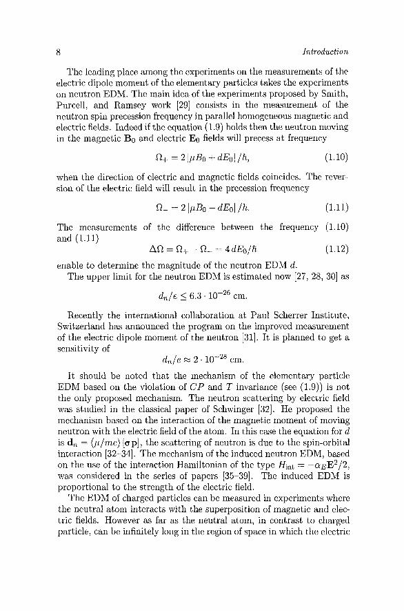
The leading place among the experiments on the measurements of the electric dipole moment of the elementary particles takes the experiments on neutron EDM. The main idea of the experiments proposed by Smith, Purcell, and Ramsey work [29] consists in the measurement of the neutron spin precession frequency in parallel homogeneous magnetic and electric fields. Indeed if the equation (1.9) holds then the neutron moving in the magnetic Bo and electric Eo fields will precess a t frequency

when the direction of electric and magnetic fields coincides. The rever- sion of the electric field will result in the precession frequency

The measurements of the difference between the frequency (1.10) and (1.11)

AS2 = R+ - R- = 4dEo/h (1.12)

enable to determine the magnitude of the neutron EDM d. The upper limit for the neutron EDM is estimated now [27, 28, 301 as

d,/e 5 6.3. cm,

Recently the international collaboration at Paul Scherrer Institute, Switzerland has announced the program on the improved measurement of the electric dipole moment of the neutron [31]. It is planned to get a sensitivity of

d,/e FZ 2 . cm.

It should be noted that the mechanism of the elementary particle EDM based on the violation of CP and T invariance (see (1.9)) is not the only proposed mechanism. The neutron scattering by electric field was studied in the classical paper of Schwinger [32]. He proposed the mechanism based on the interaction of the magnetic moment of moving neutron with the electric field of the atom. In this case the equation for d is d, = (plmc) [op], the scattering of neutron is due to the spin-orbital interaction [32-341. The mechanism of the induced neutron EDM, based on the use of the interaction Hamiltonian of the type Hint = -aiEE2/2, was considered in the series of papers [35-391. The induced EDM is proportional to the strength of the electric field.

The EDM of charged particles can be measured in experiments where the neutral atom interacts with the superposition of magnetic and elec- tric fields. However as far as the neutral atom, in contrast to charged particle, can be infinitely long in the region of space in which the electric

Experiments on search for electric dipole moment 9

field is non-zero, it should mean that the integral electric field at each individual charge of atom is equal to zero. It was shown by Schiff [40] that the non-zero electric field at atomic nucleus can be compensated by the forces of the non-electric nuclear interaction of nucleons, or by the interaction of the nucleus magnetic moment with the gradient of magnetic field produced by electrons of the atomic shells.

The experiments with the paramagnetic atoms give the possibility to measure, in principle, the EDM of electron. Sandars [41, 421 has demonstrated that when the relativistic effects are taken into account then the ratio of the atomic EDM d A to the electron EDM d , is about d A / d , % z302. This ratio can be quite large for suitable paramagnetic atoms. The reported results for the experimental limit on the size of electron EDM are [43, 441

The spin of electron shells in diamagnetic atoms is equal to zero thus the nucleus EDM can be in principle measured. In this case the nucleus spin is initially polarized by the optical methods and then the frequency of atomic spin precession in the collinear magnetic and electric fields is measured. The principle idea of the method is the same that is used to measure the EDM of neutron. The upper limits for the atomic EDM of lg9Hg [45] and 12gXe [46] are

d ('"H~) /e 5 8.7. cm,

d ( 1 2 g ~ e ) /e < 0.7. cm.

If we assign the atomic EDM to the valent neutron in the even-odd nucleus of l"Hg, then the obtained data provide the estimations for the upper limit of the neutron EDM.

Concluding the discussion we can see that the series of recent experi- ments bring out clearly that the behavior of elementary particles in the processes of their interaction with the electromagnetic field does not al- ways adequately described by the basic equations of quantum mechanics. There are some specific features that require the further understanding. Indeed the magnitude of the electron magnetic moment does not coincide with the Bohr magneton, the hydrogenic spectrum differs from the spec- trum calculated on the basis of non-relativistic and relativistic equations of the quantum mechanics, etc. All these discrepancies have been already explained in the modern theory, but the reasonable coincidence between the experimental and calculated data can only be obtained if we use the quantum field theory methods. The secondary quantization procedure is certainly in close connection with the methods of quantum mechanics,

10 Introduction

nevertheless it is out of the frames of the canonical quantum mechanics. This situation stimulates some essential questions of the fundamental and applied manner. Firstly, whether these discrepancies indicate on the imperfection of the basic principles of quantum mechanics, i.e. the lack of its self-consistency, or, simply, by improving the basic equations of quantum mechanics we can get the further insight into the nature of these discrepancies. Secondly, the main difference and main advantage of the quantum field theory approach is in the account for the virtual processes. As a result the number of particles involved into the process of some incident particle scattering does not fixed, while in the frame of quantum mechanics theory the number of particles is fixed by the normalization condition. Probably it gives us some indications how we should generalize the equations of quantum mechanics. Thirdly, it is evident that the problem of electron motion in the Coulomb field is not equivalent to the hydrogen atom problem, because the hydrogen atom problem is a two-body problem. The nucleus of hydrogenlike atoms has a finite mass, most of the nuclei have the non-zero spin and magnetic moment as well. The modern spectroscopy feels reliably the effects associated with the finite mass, spin, and magnetic moment of nucleus, it gives a serious motivation to develop the methods for solving of the two-body problem. This problem is two-fold: to develop the consistent procedure of deriving of the Hamiltonian of the two-body problem, and to develop the adequate methods of the mathematical analysis of the obtained equations.

I have tried in this book to present the atomic spectroscopy theory in deductive manner by starting from the simplest models to come gradu- ally to the most general models. The book consists of the two main parts. The first part is devoted to the development of the hydrogenic spectrum theory based on the use of the Schrodinger equation, Pauli equation, Klein-Gordon-Fock equation, and Dirac equation. The comparative analysis of the spectra obtained from the solution of the above equations is given. Simultaneously, the method of deriving of the Hamiltonian for many-body problem from the equations for particle motion in the external electromagnetic field is developed. The method is based on the use of the canonical Lagrangian formalism. As an examples illustrating the main points I have tried to use the examples from the modern spectroscopy and light-matter interaction physics. The second part of the book is devoted to the development of the spin-112 particle theory. The base problems are here: (1) the energy spectrum of hydrogenlike atoms; (2) the spectrum of geonium atom; (3) the problem of electric dipole moment of spin-112 particles. The close connection between all these problems is demonstrated.

PART I

FINE AND HYPERFINE STRUCTURE OF ATOMIC SPECTRA

Chapter 2

SCHRODINGER EQUATION

The first quantum mechanical theory, that gave the explanation of the discrete spectra of atomic emission, was based on the equation proposed by Schrodinger [2] in 1927. In this chapter we discuss briefly the basic principles and main concepts of quantum mechanics. We start with the Schrodinger and Heisenberg equations, then we introduce the main quantum mechanical operators, and consider the properties of the wave functions and operators. The problem on the electron motion in Coulomb field for Schrodinger equation is analyzed in details. The analysis of the problem on the two oppositely charged particles interaction enables us to introduce the reduced mass. The concept of reduced mass plays the crucial role in the theory of atomic spectra. Finally we consider the problem on the energy spectra of atom placed in atomic trap and analyze the specific features of interaction of the trapped atom with electromagnetic wave.

2.1 Schrodinger equation To remind the basic principles of the quantum mechanics we start

here with the Schrodinger and Heisenberg equations and discuss briefly the boundary conditions for the states of discrete and continuous energy spectra for particle moving in attractive potential.

2.1.1 Schrodinger and Heisenberg equations

The first quantum-mechanical equation was proposed by Schrodin- ger [2] in 1927. The Schrodinger equation is

14 Schrodinger equation

where Ho is the Hamiltonian

p2 Ho = - + U ( r ) . 2mo

The first term in the Hamilton Ho is the kinetic energy, which depends on the momentum operator p = -ihV, and the second term is the potential energy depending on the coordinate operator r . The particle coordinate r and momentum p operators obey the following commutation relations

where i = 1,2 ,3 . The solution of equation (2.1) for the case of free particle, i.e.

U ( r ) = 0, is

$ ( r , t ) = [Ck exp ( ikr) + C-I, exp ( - ikr)] exp (-i?), k

where the energy of particle Ek in the state with the momentum hk is

the constants C*k determine the initial state of the particle and can be determined from the initial condition

$I ( I - , 0) = [G exp ( ikr) -t C-k exp ( - ikr)] k

Thus the state of the free particle is described by the superposition of plain waves, and the particle energy depends quadratically on its momentum.

The general algorithm of obtaining equation for particle interacting with the electromagnetic field from free particle equation consists in the use of the following replacements

a a 4 ih- -t ih- - qp, -ihV -+ -ihV - - A ,

at at C (2.3)

where q is the particle charge, cp ( r , t ) and A ( r , t ) are the scalar and vector potentials of the electromagnetic field, respectively. By applying the replacements (2.3) to the Hamiltonian of free particle, we get the following wave equation for the particle interacting with the electrornag- netic field

a$ (r t ) ih- = [& (p - !A) + qp] $ ( r , t ) at

Schrodinger equation 15

The eigenfunctions of the equation (2.1) enable us to determine the quantum mechanical average of the arbitrary functions f (r , p) of oper- ators r and p. The quantum mechanical average are determined by

The quantum mechanical representation in which the operators are the function of canonically conjugated operators r and p, while the wave functions are time-dependent, is called by Schrodinger representation.

Along with the Schrodinger representation the Heisenberg representa- tion is widely used in quantum mechanics. In Heisenberg representation the operators are time-dependent. The temporal evolution of the oper- ators is described by the Heisenberg equation

df 1 af - = - [f, HI + at. d t ih

If the equation (2.5) and Hamiltonian (2.2) are applied to the coor- dinate operator r then we get the following equation for the particle velocity

It is seen that the relationship between the particle velocity v and momentum p coincides with that in classical mechanics.

In the similar way, we obtain the expression for the velocity of a particle interacting with the electromagnetic field

where we have used the Hamiltonian of the equation (2.4):

The equation (2.6) shows that the operator p corresponds to the gener- alized momentum in classical electrodynamics

The generalized momentum plays an auxiliary role in classical and quantum mechanics, but in both cases the observable value is the particle velocity.

16 Schrodinger equation

This book is devoted to the study of energy spectra of the hydrogenlike atoms, therefore we shall use mainly the Schrodinger representation. The Heisenberg representation is convenient when we study the evolution of atom driving by some external electromagnetic wave. Nevertheless the Heisenberg representation will also widely used here, because it enables us to study the symmetry properties of different Hamiltonians and to define the integrals of motion. Indeed according to the equation (2.5) the operator f ( r , p ) is integral of motion if it commutcs with the Harniltonian

[f, HI = 0.

It is well known that the integrals of motion play an exceptional role in the classical and quantum mechanics.

2.1.2 Continuity equation, boundary conditions, a n d normalization condition

The equation for the bilinear combination of the wave function enable us to introduce the concept of the charge density and current density of the matter field. Multiplying both sides of equation (2.4) by complex conjugated wave function $* and subtracting from the obtained equation its complex conjugated we get

This equation can be written in the form

The equation (2.8) has the form of the classical continuity equation. Hence, the function p (r , t ) can be associated with the charge density of a particle, and the function j (r, t) plays the role of the electric current density.

Integrating the equation (2.8) over the whole space we get

Schrodinger equation 17

If the particle is in the bound state of some potential well then the current density should be equal to zero at infinity. As a result we obtain the following boundary condition at infinity

The equation (2.9) together with the boundary condition (2.10) gener- ates the following normalization condition for the wave function

1 yi (r , t)12 d~ = 1.

It is seen that the condition (2.11) means that the charge associated with the particle is always equal to the elementary charge q = & lei.

The equations (2.1) and (2.4) are the second order differential equation with respect of the space variables. Therefore to define unambiguously the radial wave function we need additionally in the second boundary condition. It is assumed usually that the wave function should be finite everywhere. For example, if we consider the particle motion in the Coulomb field it is assumed that the wave function should be finite at r = 0.

For the particle interacting with the attracting static electric and mag- netic fields, the equation (2.4) together with the boundary conditions at r -+ oo and r = 0 generates the eigenvalue problem

The eigenfunctions u, (r) corresponding to the different eigenvalues E, are orthogonal

P

uk (r) urn (r) d V = 6,,.

Usually, the particles, producing the external (with respect to consid- ered particle) fields, are located in the finite spatial volume, therefore the potentials of electromagnetic field, produced by them, tend to zero with the increase of distance: A (r)JT,, -r 0, cp (r)lT,, -+ 0. As a result, the potential energy of a particle, interacting with the external fields, is equal to zero a t r -+ oo. Hence, the energy of the bound states of particle is negative, En < 0.

If En > 0 it means that the kinetic energy of a particle at r -r

-r oo is non-zero, hence the particle can make an infinite motion. The spectrum of the positive energy eigenvalues is continuous. As far as A (r) I,,, -+ 0, cp (r)lT-, -+ 0 the solutions of the equation (2.12) have

18 Schrodinger equation

the following asymptotic form at r t oo

where k = d-/h, and X m are the spherical harmonics. The normalization condition for the wave functions of the continuous

spectrum is also determined by the equation (2.9). The general form of solution is

$J (r) = Rki (r) kim (6, V) .

The spherical harmonics are normalized by the condition

In accordance with the definition (2.8), the charge of the spherical layer (r, r + dr) is

dq = q (1 I+ r2 dfl) dr.

It is assumed that the unite charge should pass through the spherical surface of the infinite radius in the unit time. Hence

As a result the normalization condition is

1 R~Y)* (r) ~ 1 : ) (r) r2 dr = 2x6 ( k - k l ) ,

where R ~ T ) (r) is the asymptotic form of the positive energy solutions of equation (2.12).

2.1.3 Gauge transformation The equation (2.4) is gauge invariant. Indeed, if simultaneously with

the gauge transformation of vector and scalar potentials