atnas, stephanie (2010) risk preferences of doctors,...
TRANSCRIPT

Atnas, Stephanie (2010) Risk Preferences of Doctors, Lawyers and Businessmen/women: An empirical analysis. [Dissertation (University of Nottingham only)] (Unpublished)
Access from the University of Nottingham repository: http://eprints.nottingham.ac.uk/23016/1/Dissertation_stephanie_atnas.pdf
Copyright and reuse:
The Nottingham ePrints service makes this work by students of the University of Nottingham available to university members under the following conditions.
This article is made available under the University of Nottingham End User licence and may be reused according to the conditions of the licence. For more details see: http://eprints.nottingham.ac.uk/end_user_agreement.pdf
For more information, please contact [email protected]

1
Risk Preferences of Doctors, Lawyers and Businessmen/women:
An empirical analysis
By
Stephanie Atnas
2009
A Dissertation presented in part consideration for the degree of
"MA RISK MANAGEMENT".

2
Acknowledgements
I would like to thank my dissertation supervisor Mr Paul Fenn, professor in the University of
Nottingham for all his help and support during the completion of this research study.
Furthermore I would like to thank the law firms, corporations and hospitals that have
participated in this research, and all the participants that took part for their time and effort,
without their help this dissertation would not have been possible.

3
Table of contents:
Page Number
Cover page..................................................................................................................................1
Acknowledgements....................................................................................................................2
Contents page..........................................................................................................................3-4
Summary....................................................................................................................................5
Chapter one: Introduction.....................................................................................................6-9
Chapter two: Literature Review
2.1 Introduction:.......................................................................................................................10
2.2 What is risk?.................................................................................................................10-14
2.3 Theoretical background.................................................................................................15-23
2.4 Empirical Findings........................................................................................................23-35
2.5 Conclusions........................................................................................................................35
Chapter three: Methodology
3.1 Introduction: .................................................................................................................36-37
3.2 Hypothesis.........................................................................................................................37
3.3 Sample...............................................................................................................................37
3.4 Selection.............................................................................................................................38
3.5 Distribution........................................................................................................................38
3.6 Data collection .............................................................................................................39-40
3.7 Mode of questioning.....................................................................................................40-41
3.8 Pre testing......................................................................................................................41-42
3.9 Data coding and analysis....................................................................................................42

4
Chapter four: Findings and Data Analysis
4.1 Descriptive Statistics.....................................................................................................43-53
4.2 Hypothesis Testing........................................................................................................53-65
Chapter five: Discussion
5.1 Findings.............................................................................................................................66
5.2 Discussion.....................................................................................................................67-74
Chapter six: Conclusions:
6.1 Conclusions...................................................................................................................75-77
6.2 Limitations and Recommendations....................................................................................78
6.3 Reflections.........................................................................................................................79
References: ........................................................................................................................80-86
Chapter seven: Appendices
Appendix 1: Questionnaire.................................................................................................87-90
Appendix 2: Doctors.........................................................................................................91-102
Appendix 3:Lawyers.......................................................................................................103-115
Appendix 4: Businessmen/women..................................................................................116-128

5
Summary:
The aim of this dissertation is to investigate the differences in risk preferences of doctors,
lawyers and businessmen/women. Using an experimental approach, 108 questionnaires were
collected from doctors, lawyers and businessmen/women in Cyprus. After reviewing the
limited literature up to date on risk preferences in occupation, the main findings indicate that
there are differences in risk preferences amongst these three professions. Specifically,
doctors are more risk averse than lawyers and businessmen. Also, this research finds no
evidence of gender and age significant differences in risk preferences amongst professionals.

6
Chapter One: INTRODUCTION
Coming to the end of my master’s degree, as partial fulfilment of the requirements of
the MA Risk Management, I have chosen to do a dissertation on risk attitudes among
lawyers, businessmen and doctors. I have chosen to write and research this topic area not
only because it is of great interest to me; but also because risk is part of human life. Therefore
I believe that it is important to understand how different people view risk and in order to deal
with it. Researching how individuals respond and manage risk is imperative as it is
individuals who implement and deal with risk management techniques. This has received
increased importance nowadays, as one could argue that risks have become more
sophisticated, have increased in numbers, frequency and severity. This is evident as corporate
disasters are prevalent and the economy is in distress, it is apparent that risk management
techniques have failed to meet their objectives.
The aim of this dissertation is to contribute to existing knowledge on risk
management and may be used by managers, consultants and anyone interested in
understanding what determines risk behaviour and how it should be managed.
In order to gather answers that will give an in depth knowledge on this specific topic
and contribute to existing literature I have formulated a series of research questions. The
intention of this dissertation is to understand:
1) What are each groups attitudes to risk? Do attitudes vary between groups? (knowledge
and experience?)
2) What determines these attitudes?
3) Does age and gender affect risk preferences in each occupation?

7
A literature review will follow after the introduction. The literature review is divided
into three parts. The first part attempts to explain what is meant by risk, the second part
reviews theories such as the Expected Utility Theory, Subjective Utility Theory, and also
reviews psychological approaches to risk attitudes. The third part aims at reviewing empirical
studies on risk attitudes. This dissertation attempts to fill in gaps of the existing literature.
Most research in this field tends to consider mainly gender, age, and income as variables that
determine risk attitudes. There is limited research in determining differences in risk attitudes
among different professions (i.e. accountants survey, national registry of charted
accountants); this dissertation aims at introducing a new research group and expand on the
existing literature.
Following the literature review, a set of hypothesis is provided. Ho will be that there
is no difference between the groups and Ha will be that there are differences between groups.
The dissertation will then discuss the methodology that will be used to research this
topic. Previous studies on this topic adopted a positivism approach and used a quantitative
paradigm. This research aims at following the same approach taken by traditional studies.
Most approaches used to assess the importance and nature of risk aversion, in other words to
measure risk involve lottery choice data from field experiments, laboratory experiments,
bidding and pricing tasks, buying and selling prices for simple lotteries (Holt and Laury,
2002). This research takes the form of a survey. This method is chosen as is enables
comparison to be made with previous findings; it is relatively cheap and favourable
considering the time constrains. Moreover, surveys identify attributes of a population from a
small group of individuals (Sudman and Bradburn, 1986).

8
The survey was accomplished thorough questionnaires. The first part of the
questionnaire involves asking general risk questions, aiming at understanding how
individuals see themselves, in other words what they believe their risk attitude is. The second
part involves hypothetical questions which according to pervious literature usually take the
form of a standard lottery question. The aim is to examine what the individual’s risk attitude
would be, given a hypothetical scenario (this makes it possible to estimate the coefficient of
relative risk aversion for each individual, could be used as a benchmark). Finally, the third
part of the questionnaire involves real life questions (i.e. questions about willingness to take
risks in specific domains, situations). The aim here is to confirm the hypothetical attitudes
from section two.
The sample of this dissertations are medical, law and business professionals and
students. This sample was chosen as it will allow comparison to be made between
professions. Moreover it allows for comparison to be made between age and gender (to
determine whether different variables for people in the same field affect risk attitudes).
Distribution was made in corporations, law Firms, clinics, hospitals and private practices in
Cyprus. Questionnaires were also distributed to law students, medical students and business
and management students from the University of Leicester, and the University of
Nottingham.
After obtaining and analyzing the data, a discussion of findings is provided. The aim
here is to review the findings and compare them with the literature review. The main findings
of this dissertation is that Ho: there is no difference between risk preferences among
professions, is rejected. Specifically, businessmen/women appear to be less risk averse than
lawyers and doctors. Also gender and age are not significant in determining risk preferences
within occupations.

9
Finally, this dissertation draws onto some conclusions; and also acknowledging the
fact that no research is perfect, this dissertation provides a reflection and recommendation by
evaluating my work, how I might have done it differently if I was to do it again and provide
recommendations for further research.
10
Chapter Two: LITERATURE REVIEW
2.1 Introduction:
This chapter is structured in four parts. The first part is aimed at providing an
understanding of what is meant by risk. This is achieved by defining risk, introducing
background onto individuals risk preferences and how individuals depending on what their
risk preference is chose to manage risks. The second part reviews theories that are considered
as principle in the discipline of risk attitudes and decision making under uncertainty. The
third part of this chapter reviews empirical studies that have been conducted throughout the
years in respect of this topic. Finally, this chapter draws on some concluding thoughts.
2.2 What is risk?
It is important to begin this discussion by defining what is meant by the word ‘risk’.
Risk is defined according to the ISO/IEC Guide 73 as ‘the combination of the probability of
an event and its consequences (2002:2). ‘The term risk can have a negative perspective which
is the possibility of physical harm/detriment/ loss due to a hazard. Risk can alternatively
adopt a neutral perspective which is the uncertainty about the outcome of a decision; or it can
adopt a positive perspective where risk is regarded as a thrill’ (Rohrmann, 2004:2). It must be
noted, that as risks are found in many disciplines such as medicine, engineering,
management, law, psychology, something it is possible to find that risks are defined
differently, in order to reflect the discipline they represent.
Historically risk, was defined as uncertainty, Frank Knight in 1921 was the first to
make a distinction between risk and uncertainty. According to Knight risk is quantifiable and
measurable whereas uncertainty is not. Knight however failed to provide an explanation of
how risks should be measured, that is whether probability value should be used or a variation

11
measure (Houston, 1964). Pfeffer (1956) argued that ‘risk is a state of world whereas
uncertainty is a state of mind’ (p42), therefore risk should be measured by objective
probability and uncertainty should be measured by subjective degree of belief.
Individual risk preferences:
Different individuals adopt different attitudes towards the risks they are exposed to.
Individual risk attitudes is defined as ‘a generic orientation towards taking or avoiding a risk
when deciding how to proceed in situations with uncertain outcomes’ (Rohrmann, 2004:2). It
must be noted that risk attitudes is different from risk behaviour which is ‘the actual
behaviour of people when facing a risk situation’ (Rohmann, 2004:2) and is different from
risk perception which is defined as ‘a person’s judgement about how large the risk associated
with a hazard is’ (Rohmann, 2004:2)
Individual risk preferences tend to be determined by one’s gender, age, education,
religion, family background, intelligence, social environment, experiences, events as well as
other variables (Greene, 1971). Risk preferences may also be affected by mood (Hastorf and
Isen, 1982), feelings (Jhonson and Tversky, 1983) as well as the way in which risks are
framed as suggested by Tvesky and Kahneman, (1981). Tversky and Kahneman (1981) argue
that ‘when dealing with a risky alternative whose possible outcomes are generally good,
human subjects appear to be risk averse; but if they are dealing with a risky alternative whose
possible outcomes are generally poor, human subjects tend to be risk seeking’ (obtained from
March and Shapira, 1992:1406).
‘Individuals risk preferences may be viewed as falling somewhere on a risk
continuum that ranges from feelings of extreme dislike of risk to feelings of acceptance and
even desire for risk’ (Greene, 1971:12). James Tobin (1958) introduced the idea that
individuals risk preferences are classed into risk averse, risk neutral, or risk loving.

12
According to Tobin (1958) an individual is said to be risk averse, that is the individual tends
to dislike risks, if for any probability distribution the individual prefers the expected value of
the distribution to the distribution itself. In other words according to Tobin (1958), ‘risk
averters will not be satisfied to accept more risk unless they can also expect to gain more
return’ (obtained from Greene, 1971:33) An individual is said to be risk neutral, if for any
probability distribution the individual is indifferent between the expected value of the
distribution and the distribution itself. Finally, an individual is said to be risk loving, if for
any probability distribution the individual prefers the distribution to its expected value. In
other words, according to Tobin (1958), ‘risk lovers are willing to accept lower expected
return in order to have the chance of unusually high capital gain’ (obtained from Greene,
1971:33). Moreover, according to Greene (1971), ‘the risk averter, seldom takes unnecessary
chances, he is conscious of risk, tends to plan carefully, whereas the risk lover is the exact
opposite’ (p12).
It is important to understand individuals risk attitudes because ‘risk attitude is a
source of significant bias on decision making and the effectiveness of the risk management
process. It follows that to improve risk management it is important to understand risk
attitudes’ (Hillson and Murray-Webster, 2006:25). This is because, ‘risk management is
undertaken by people, acting individually and in groups, with a multitude of influences both
explicit and covert. People adopt risk attitudes which affect every aspect of the risk process
even if they are unaware of it. Understanding and managing these attitudes would
significantly increase risk management effectiveness’ (Hillson and Murray-Webster,
2006:25), which is critical now more than ever as ‘risk management has proven to fail to
meet its expectations as demonstrated by repeat corporate failure’ (Hillson and Murray-
Webster, 2006:25).
13
It must be noted that risks may occur voluntarily or passively. Individuals may be
exposed to risks passively, that is as a result of inability to predict or identify a risk; or
voluntary, that is as a conscious decision often as a result of risk offering pleasure to the
individual. Moreover, it needs to be said that individuals may adopt an active or a passive
stance towards risk management. According to a study by March and Shapira, (1987) who
confirmed previous study of MacCrimmon and Wehrung, (1986) find that ‘with the passive
approach, managers selected only from the alternatives that were available to them whereas
under the active approach managers tried to adjust the components of the risky situation by
gaining time, gathering information or increasing their control over the decision’ (Helliar,
2001:13)
Methods of handling risks:
Once individuals acknowledge the fact that they are exposed to a risk the next step is
most likely to engage in risk minimization activities. ‘Conventional decision theory assumes
that decision makers deal with risk by first calculating and then choosing among alternative
risk-return combinations that are available’ (March and Shapira,1992:1406). The way in
which an individual chooses to deal with risk will be determined by the individual’s risk
preference. For example a risk averse individual will most likely choose to respond to a risk
immediately whereas the risk lover may take a passive stance. It must be said that as ‘the
concept of risk has been a concern of human beings from the earliest days of recorded history
and most likely even before that’ (Gier, 1980; 198, obtained from Trimpop, 1994:1),
individuals have long engaged in risk minimization and risk management activities in order
to protect themselves. ‘The earliest evidence of risk management can be traced in the marine
insurance nearly 3000 years ago’ (Bernstein, 1996:4), ‘risk management is also evident in the
Old Testament in the Middle Ages when hedging was used to create future markets’ (Froot et

14
al, 1994:92). According to Bernstein (1996) ‘risk management was used in medieval and
ancient words even in preliterate and peasant societies; to make decisions, advance their
interest and carry out trade’ (p2-4). There are many ways by which risks can be dealt with.
To begin with, ‘assuming a risk or doing nothing about the certainty to which one is
exposed is probably the most common way of dealing with risk’ (Greene, 1971:18). Adopting
a passive stance towards risk implies that individuals accept the risk (Weinsein, 1980). ‘An
individual will assume a risk when the probability of loss is extremely small and there is not
economic reason for not assuming the risk, or when there is no other significant reason for
taking any action against it (Greene, 1971:19). Furthermore, an individual may decide to
transfer the risk to a third party, usually to an insurance company that provides compensation
in the loss state, in exchange for a premium that is payable regardless of which state of the
world materialized. Alternatively, an individual may decide to diversify the risk. Moreover,
loss prevention and loss reduction may be used to handle risk, especially when the risk may
impose financial costs. This implies that individuals engage in risk minimization activities
such as installing sprinkler alarms, burglar alarms and fire alarms. The former aims at
reducing the probability of a loss occurring in the first place whereas the second implies that
the size of the loss is reduced. It is better that risks are handled immediately, in order to avoid
building pathogens which lead to disaster as suggested by Turner (1994).

15
2.3 Theoretical background:
Expected Value Theory was developed by Blaise Pascal in the 17th
century.
According to this theory ‘individuals evaluate risky prospects by their expected value.
Therefore any decision maker should accept to pay an infinite amount of money for prospects
with an infinite expected value’ (Pfieffelmann, 2007:2). Expected value however, considers
only the size of the payout and the probability of occurrence. This drawback, lead to the
famous St Petersburg Paradox, developed by Nicholas Bernoulli (1713). This paradox is
represented by a lottery game in which an individual tosses a fair coin repeatedly until it falls
on heads. The gambler will get £1 if this happens the first time, £2 if this happens the second
time, £4 if this happens the third time, £8 if this happens the fourth time and so on.
Mathematically it can be represented as: E(G)= ½. 2+ ¼.4+..............+2¯ˆK . 2ˆK= (1+1+.....)=
00 (Cowen and High, 1988:219). ‘The St Petersburg Paradox shows that for prospects with
infinite expected monetary value decision makers are not willing to pay an infinite sum of
money. According to a number of experiments the maximum price on individual is willing to
pay for this gamble is 3 Euros. This observation can be taken as evidence against expected
value’ (Pfiffelmann, 2007:2).
Daniel Bernoulli (1738) analyzed the paradox in the commentaries of the Imperial
Academy of Science of St Petersburg, and provided a solution to it. ‘Daniel Bernoulli solved
the paradox by introducing the idea of diminishing marginal utility. He postulated that
individuals valuate prospects not by their expected value but by their expected utility where
utility is not linearly related to outcome but increases at a decreasing rate. Therefore, if it is
considered that individual’s preferences are represented by a strictly increasing and concave
utility function this paradox is resolved’ (Pfiffelmann, 2007:2).
16
‘Since Daniel Bernoulli solved the St Petersburg Paradox, Expected Utility Theory
has been considered as a benchmark for describing decision making under risk’ (Pfiffelmann,
2007:2). ‘Expected Utility Theory has been used in Economics as a descriptive theory to
explain various phenomena such as the purchase of insurance and the relation between
spending and saving; and has also been employed as ‘a normative theory in decision analysis
to determine optimal decision and policies’ Tversky, 1995:1). In other words Expected utility
theory builds on the possibility that individuals can have different attitudes to risk.
‘Expected Utility Theory was first axiomatized by Von Neumann Morgenstein
(1944), who introduced the utility function to explain individual preferences’ (Beberau,
1964), in other words in order to understand peoples risk attitudes, an utility function is
adopted. Expected Utility theory was further developed by Savage (1954) who integrated the
notion of Subjective probability into Expected Utility Theory’ (Tversky, 1975:1).
According to the Expected Utility Theory, ‘choices are coherently and consistently
made by weighing outcomes (gains or losses) of actions (alternatives) by their probabilities
(with payoffs assumed to be independent of probabilities’ (Sebora Terrence, 1995:4). In other
words, individuals will choose among the option that yields the highest utility, ‘utility being
all of the psychological, economic, sociological, philosophical, and other factors that enter
into a person’s subjective assessment of the uncertainties that affect his financial future’
(Greener, 1971:25) with respect to the size of the payout, the probability of occurrence,
individuals risk aversion and the utility obtained according to ones financial ability and
personal tastes. Expected Utility Theory is based on three fundamental tenets about the
process that occur during decisions made under risk and uncertainty: 1) consistency of
preferences for alternatives, 2) linearity in assigning of decision weights to alternatives, and
3) judgement in reference to a fixed asset position. Based on these assumptions Expected
Utility predicts that the better alternatives will always be chosen’ (Sebora Terrence, 1995:4).
17
The axioms of Expected Utility Theory are considered as ‘principles of
individual rational behaviour under uncertainty’ (Tversky, 1975:1). In other words, the
axioms of Expected Utility Theory can describe an individual’s risk attitudes. However,
Expected Utility Theory Axioms have received considerable criticism over the years due to
the controversy that exists between experimental studies that test the validity of the axioms
leading to questioning whether these axioms are legitimate in explaining individual behaviour
under risk and uncertainty. Studies by Tversky, (1951), Raffia, (1968), Lichtenstein, (1968),
Kahneman and Tversky, (1973) find evidence of violation of these axioms whereas Mosteller
and Nogee, (1951), Davidson et al, (1957), Tversky, (1967) find evidence that the axioms are
not violated and support Expected Utility Theory.
The experimental studies that report persistent violations of Expected Utility find that
‘on the one hand individuals preferences for insurance lead to risk averse behaviour whereas
on the other hand acceptance of gambling indicates risk seeking behaviour’ (Pfiffelmann,
2007:2) an observation which was initially made by Friedman and Savage (1948). The fact
that individuals engage at the same time in two conflicting behavioural choices gave rise to
the Subjective Expected Utility theory which suggests that ‘people choose their risk taking
behaviour in relation to potential gains and losses based on absolute amounts’ (Trimpop,
1944:119). In other words, Subjective Expected Utility prospects that forming the value of a
prospect that involves risk, people weigh the outcomes by decision weights that are functions
of probabilities rather than the objective probabilities’ (Harbaugh, Krause, Vesterlund,
2002:54)
Friedman and Savage (1948) argued that ‘this conduct is viewed as inconsistent
because the expected marginal utility of the game would seem to be less than the marginal
utility of the stake’ (Greener, 1971:27). To illustrate their argument they developed the
‘utility curve’ which takes an S shape. The S shape of the utility curve is concave at low

18
wealth levels and convex at higher wealth levels. This implies that for intermediate amounts
of wealth individuals indicate risk-loving behaviour (convexity), while for large or small
amounts of wealth individuals indicate a risk averse behaviour (concavity) (Just and Lybbert,
2009). What this essentially entails is that ‘wealthy individuals are more conservative with
their money and tend to be large purchasers of insurance’ (Greener, 1971:29).
However, what followed the Friedman and Savage classical paper was a series of
criticisms. Initially Markowitz (1952) modified Friedman and Savage argument. Using
experimental evidence he suggested that ‘a second convex segment is present at the lower
and end of the utility function and that the middle inflection point of the resulting function is
near the individual’s present wealth level’ (Hakansson, 1970:472-3). Furthermore, Menahem
Yaari (1965) who also tested the Friedman and Savage hypothesis found no evidence of a
convex segment in the utility function. He argued that the presence of simultaneous insurance
and gambling behaviour was attributed to the fact that low probabilities are overestimated
and high probabilities are underestimated. Yaari (1965) argument was supported by M.G
Preston and P. Baratta (1948), F.Mosteller and P.Nogee (1951). Moreover, Ward Edwards
(1954) argued that ‘the Friedman and Savage hypothesis cannot succeed if certain
probabilities were preferred over probabilities in gambling experiments. Edwards objection to
the existence of any simple method of measuring utility was supported since other
investigators have found that factors such as personality variables, education levels, age and
intelligence enter into one’s willingness to take risk’ (Greener, 1971:30-1) However Richard
Rosset (1967) opposed Yarri’s (1965) findings that the Friedman and Savage model does not
stand. He suggested that this was the case because ‘the subjects may have been engaged in
prior unresolved gambles at the time of experiment’ (Hakansson, 1970:473). ‘Jack
Hirshleiffer (1966) also argued that utility functions of money are concave throughout; he
attributes the acceptance of unfavourable bets to the pleasure or consumption value of

19
gambling’ (Hakansson, 1970:473). Raiffa (1968) expanded on the Friedman and Savage
hypothesis and argued that ‘ the utility function that a person works with today should be
sensitive to the demands or investment opportunities that he perceived will be available to
him in the future’(Raiffa, 1968:96 obtained from Hakansson, 1970:473-4).
Measuring Risk Aversion:
As already mentioned ‘according to the Expected Utility Theory, the dollar amount
and the proportion of risky asset in an investors portfolio are assumed to be a function of the
person’s wealth and degree of risk aversion. A person’s degree of risk aversion is in turn
assumed to depend on their wealth’ (Jianakoplos and Bernasek, 1998:622). Pratt (1964) and
Arrow (1971) were the first to presented the relationship between risk preferences and wealth
and presented the measures of risk aversion, both absolute risk aversion and relative risk
aversion. Absolute risk aversion determines how utility changes with absolute changes in
monetary amount of risky assets in a portfolio whereas the relative risk aversion determines
how utility changes with proportional changes of risky assets in a portfolio. Evidence
indicates that absolute risk aversion decreases with wealth but there is no evidence that this is
the case in relative risk aversion (Jianakoplos and Bernasek, 1998).
Friend and Blume (1975) further developed a framework to measure relative risk
aversion on which a number of empirical studies on risk aversion relied upon. In their model,
Friend and Blume (1975) ‘explain the division of an individual’s portfolio between risky and
risk free assets, in the absence of taxes’ (Jianakoplos and Bernasek, 1998:622). Their aim is
to measure how the coefficient of relative risk aversion varies with wealth.
It must be noted that there are problems associated with measuring risk aversion.
According to Hartog et al (1998), these include ‘sensititvity to framing, elicitation bias,
preference reversal and the gap between willingness to pay and willingness to accept’(p4).

20
Moreover, the Parat-Arrow measure of risk aversion has been criticised on the grounds that
the risk aversion of the same individual may be different depending on how big the change in
utility is.
Psychological approaches to decision making under uncertainty (Critique of EUT):
Experimental studies increasingly indicate violations of Expected Utility Theory;
consequently alternative theories were developed that are ‘more psychologically appealing
and more valid’ (Rieger and Wang, 2006:666). Tversky and Kahneman developed the
Cumulative Prospect Theory in 1992, which can be argued ‘stands out as one of the most
well accepted descriptive alternatives to Expected Utility Theory’ (Rieger and Wang,
2006:666). ‘The Cumulative Prospect theory, introduced the use of decision weighs to
account for the value functions in risky choices’ (Trimpop, 194:119). It is based on four
features: ‘1) instead of evaluating the wealth, the payoffs are framed as gains or losses as
compared to some reference point; 2) the sensitivity relatively to the reference point is
decreasing. The value function is then concave for gains and convex for losses; 3) individuals
have asymmetric perception of gains and losses, they are loss-averse, hence the value
function in losses is steeper than the value function in gains; and 4) individuals do not use
objective probabilities when evaluating risk projects. They transform objective probabilities
via a weighting function. They overweigh the small probabilities of extreme outcomes and
underweigh outcomes with average probabilities’ (Rieger and Wang, 2006:666, Pfiffelmann,
2007:2).
According to Kahnemman and Tversky, this behaviour is a result of two human
shortcomings. ‘First, emotion destroys the self-control that is essential to rational decision-
making and second, people are often unable to understand fully what they are dealing with.
They experience what psychologies call cognitive difficulties’ (Benrstein, 1996:271).

21
Prospect theory was supported by Schurr (1987) who through experimental research ‘showed
that groups of professional buyers reacted to situations framed as potential losses with risk
seeking and to situations framed as potential gains with risk averse behaviour’ (Trimpop,
1994:119). Similarly, Levy and Levy (2002) experimental study which aimed at comparing a
positive prospect with a certain outcome; and compared a negative prospect with a certain
negative outcome found that 81% of the choices in the first task were consistent with risk
aversion for gains and 69% of the choices in the second task were consistent with risk
seeking for losses. This finding was similar to the findings by Kahneman and Tversky (1979)
who found 80% and 92% respectively (Levy and Levy, 2002).
The Cumulative Prospect Theory however received criticisms and was argued that it
is subject to limitations. Blavatsky (2005) argued that ‘the overweighting of small
probabilities can lead to the re-occurence of the St Petersburg Paradox. He showed that the
valuation of a prospect (the subjective utility) by Cumulative Prospect Theory can be infinite’
(Pfiffelmann, 2007:2). ‘As already mentioned the St Petersburg Paradox can be resolved by
introducing a concave utility function. The game however can be modified so that the
concavity of the utility function is not sufficient to guarantee a finite utility value. Arrow
proposed to resolve this problem by only considering distributions with finite expected value.
In that case, the concavity of the utility function is sufficient to guarantee, under Expected
Utility framework a finite valuation’ (Pfiffelmann, 2007:3).
Rieger and Wang (2006); Pfiffelmann (2007), pointed that ‘under Cumulative
Prospect Theory with finite expected value can have infinite subjective utility’ (Pfiffelmann,
2007:8), something that emphasises the importance of increase overweighting at decreasing
probabilities. ‘Rieger and Wang (2006) focused on fifty parameterized functional forms to
Cumulative Prospect Theory functions and determined for which parameter combinations the
model implies finite subjective value for all lotteries with finite expected value’ (Pfiffelmann,
22
2007:8). Rieger and Wang (2006) further suggested another solution to the paradox under
Cumulative Prospect Theory. They proposed to ‘consider polynomial of degree tree as a
weighting function; as its slope at zero is infinite, this weighting function permits to avoid
infinite subjective utilities for all prospects with finite expected value’ (Pfiffelmann, 2007:9).
It can be argued that this solution to the paradox problematic, this is because it entails
behavioural implications as it does not allow for betting on unlikely events neither does it
allow for insurance on unlikely losses (Pfiffelmann, 2007). Pfiffelmann (2007) attempted to
resolve this paradox in rank dependent model, by suggesting an alternative weighting
function whose slope at zero is not infinite (Pfifelmann, 2007). Moreover, according to
Grossberg and Gutowski, 1987), it can be argued that ‘the prospect theory in contrast to
subjective utility theory is an algebratic, static theory that relies on group choice data.
Therefore it does not account for individual decisions or information processing that
underlies decision making under uncertainty’ (Trimpop, 1994:119).
Willingness to pay/ willingness to accept:
Along the same lines, Horowitz et al (2000) state that ‘previous authors have shown
that willingness to accept is usually substantially larger than willingness to pay, and most
have remarked that the willingness to pay/willingness to accept ration is much higher than
their economic intuition would predict’ (obtained from Plott and Zeiler, 2005:531). One
interpretation of this gap is the endowment effect which ‘rests on a special theory of the
psychology of preferences associated with prospect theory’. In particular Jack L Knetsch et al
(2001) conclude that ‘the endowment effect and loss aversion has been one of the most robust
findings of the psychology of decision making: people commonly value losses more than
commensurate gains’ (obtained from Plott and Zeiler, 2005:531).
23
Because there is a variation in experimental results of willingness to pay and
willingness to accept, the argument that it is due to the fact that the endowment effect is
questioned and another interpretation of this gap is provided. It is argued that this is a result
of a failed and problematic experimental methodology. In other words, it is a result of a series
of misconceptions and confusions. This argument was supported by Plott and Zeiler (2005)
who control for misconceptions by ‘ensuring anonymity, using incentive-compatible
elicitation, provide subjects with practice and training on the elicitation mechanism before
employing it to measure valuation’ (p 530) and find evidence that the willingness to pay –
willingness to accept gap is not a result of human preferences.
2.4 Empirical evidence:
Most empirical research in risk attitudes adopt either a field or laboratory
experimental approach, bidding and pricing tasks, buying and selling prices for simple
lotteries (Holt and Laury, 2002). Experimental research may take an abstract gamble
approach or a context environment approach. In abstract experiments framing affects
decision, whereas in context experiments psychology attitudes change according to the
environment. To measure risk attitudes most empirical evidence conducted tend to ‘examine
which individual’s behaviour is consistent with expected utility maximization’ (Eckel and
Grossman, 2008:3). ‘It must be noted that risk attitudes tend to vary over environments with
low levels of correlation across tasks, measures and context’ (Eckel and Grossman, 2008:3).
As already mentioned ‘the nature of risk aversion is an empirical issue. Therefore,
laboratory experiments can produce useful evidence that compliments field observations by
providing careful controls of probabilities and payoffs. However, low laboratory incentives
may be somewhat unrealistic and therefore not useful in measuring attitudes toward ‘real-

24
world risk’ (Holt and Laury, 2002:1644). Kahneman and Tversky (1979:265) suggest an
alternative: ‘experimental studies typically involve contrived gambles for small stakes, and a
large number of repetitions of very similar problems. These features of laboratory gambling
complicate the interpretation of the results and restrict their generality. By default the method
of hypothetical choices emerges as the simplest procedures by which a large number of
theoretical questions can be investigated. The use of the method often relies on the
assumption that people often know how they would behave in actual situations of choice, and
on the further assumption that the subjects have no special reason to disguise their true
preferences’ (obtained from Holt and Laury, 2002:1645).
According to Anderson and Brown (1984), who attempt to investigate ‘the importance
of excitement in gambling, the effects of runs of wins and losses on gambling behaviour and
the relationship of both sensation-seeking using samples of students and experienced
gamblers in real and artificial gambling situations’ (Anderson and Brown,1984:401) found
that individuals behave differently in laboratory experiments, than they would in real life.
Specifically they find that, ‘gambling behaviour in terms of both the degree of risk assumed
and the strategy of decision making in circumstances of runs of wins and losses differs to a
significant degree in the real and the laboratory situations’ (Anderson and Brown, 1984:407).
According to Anderson and Brown the problem with laboratory studies in gambling is
that they lack credibility, ‘hidden interactions which occur in real life situations are ignored
in the laboratory’ (Anderson and Brown, 1984:401). A persons willingness to take risks will
depend on the motivations (i.e. whether there are financial gains), as in laboratories
individuals will not have financial gains and are dealing with money that will not affect their
life they are likely to behave differently. To deal with this, ‘many studies have attempted to
generate excitement by trying to induce competition among participants by setting up prizes
(e.g. Ginsburg et al, 1976, Kuhlman, 1976) or trying to generate a competitive atmosphere

25
between male and female subjects (Rule and Fischer, 1970), but in most real gambling
situations the essence of the game is that participants play against the house, dealer or
bookmaker- not against each other. Also in a ‘prize situation’ where participants are aware of
how much others are winning , little or no excitement is generated for a particular subject
who is far behind another that he or she cannot possibly catch up’ (Anderson and Brown,
1984:401). ‘Or more excitement than is appropriate may be generated if the only way to catch
up would be to take a series of great risks, producing a bias inherent in the experimental
situation for greater risk taking when subjects are behind. Thus attempts to compensate for
the lack of excitement due to limited or no monetary risk in the laboratory may seem
reasonable but, under close scrutiny actually add to the artificiality of the situation’
(Anderson and Brown, 1984:401).
Moreover it can be argued that, ‘laboratory studies tend to fact that different
individuals adopt different risk taking behaviours which is largely determined by personality
traits’ (Rule and Fischer, 1970; Rule et al, 1971; Hatano and Inagaki, 1977, obtained from
Anderson and Brown, 1984). Friedman and Sunder (1994:44) expand this argument and
support the idea that ‘reliable demographic data on individual risk attitudes is virtually
nonexistent’. It can be argued that this statement is correct; as although there have been a lot
of research throughout the years on risk attitudes such as Eckel and Grossman (2008); Holt
and Laury (2002); Harrison and Rutstrom (2002); Harrison et al (2003); Bajtelsmit and
VanDerhei (1997) as well as others, there is very little empirical evidence that considers
individual characteristics such as income, type of work, age, ethnicity. Most empirical
evidence in the theory of risk aversion tends to focus on gender differences in risk aversion,
some of which combine it with other variables such as number of dependents, and race. Most
literature on gender differences in risk aversion argue that women are more risk averse than

26
men (Levy, Elron, Cohen (1999); Powell and Ansic,(1997); Eckel and Grossman, (2008);
Levin, Snyder and Chappman, (1998)).
Powell and Ansic, (1997) furthermore argue that, ‘experimental studies which use
gambling examples are appropriate in terms of gains and losses for financial decision making,
but lack salience (Butler and Hey, 1987), if they do not involve real winnings. In addition,
experimental gambles have been seen to have limited generality because they produce
different results when compared to real betting’s (Anderson and Brown, 1984; Wagenaar,
1988). Even when real betting data are used, gambling involves an element of utility derived
from leisure (as distinct from the utility associated with wining money) which may not be
reflected in financial decision (Johnson and Bruce, 1992)’. (Powell and Ansic, 1997:610).
Holt and Laury (2002), measure risk aversion using lottery choices under real and
hypothetical situations. They find that ‘with real payoffs, risk aversion increases sharply
when factors are scaled up. This result is qualitatively similar to that reported by
Kachelmeirer and Shehata (1992) as well as Smith and Walker (1993). In contrast, behaviour
is largely unaffected when hypothetical questions are scaled up’ (Holt and Laury,
2002:1653). The authors argue that these results may be explained by considering the
assumption that ‘subjects facing hypothetical choices cannot imagine how they would
actually behave under high incentive conditions. Moreover, these differences are not
symmetric; subjects typically underestimate the extent to which they will avoid risk. Second,
the clear evidence for risk aversion even with low stakes, suggests the potential danger of
analyzing behaviour under the simplifying assumption of risk neutrality’ (Holt and Laury,
2002:1654).
Brinig (1995) examines using abstract gamble experiment that does not involve any
loss, whether gender and age affect individual risk preferences. Brinig (1995) finds no
evidence of gender difference in risk preferences, but when gender is integrated with age she

27
finds differences in risk preferences. She finds that females are more risk averse than males
from the onset of adolescence to the mid forties; then they are less risk averse until the age of
forty-five, and beyond that age both genders exhibit the same risk preferences. As Brinig
(1995) notes, ‘this finding is consistent with the sociobiologists hypothesis that men are
relatively more risk loving during the period in which they are trying to attract mates, while
women tend to be more risk averse during their child bearing years’ (Eckel and Grossman,
2008:5). Brinig (1995) finding however has been criticised as participants faced no loss
(Bajtelsmit, et al 1999).
Harbaugh, Krause, Vesterlund, (2002), using an abstract gamble experiment
researched whether age impacts of individuals’ risk attitudes. To achieve this they used a
sample of 234 participants (children, teenagers, college students and adults), which were
provided with real incentives and simple choice procedures from which they were required to
evaluate fourteen choices between a simple gamble and a certain outcome (Harbaugh,
Krause, Vesterlund, 2002). The study found that ‘70% of children chose a fair gamble when
the outcome of the gain was 0.8 while only 43% of adults did. Over losses, 75% of children
took a fair gamble when the chance of loss was 0.1 compared to 53% of the adults. Adults
choices are seen to be consistent with their use of objective probabilities when evaluating a
gamble over a gain, however when evaluating a gamble over a loss they use subjective
weighs. On the other hand, the within subject analysis revealed that the proportion of
participants with a regressive weighting function increases with age’ (Harbaugh, Krause,
Vesterlund, 2002:72). This study also revealed that ‘the probability weighting functions
changes with age. Specifically, children’s decisions are consistent with the use of large
subjective probability weights and these weights decrease with age. Also, children and
youngsters were seen to underweight low probability events’ (Harbaugh, Krause, Vesterlund,
2002:73).

28
The Schubert, Gyster, Brown and Brachinger (1999), and Moore and Eckel (2003)
study gender differences in risk attitudes by adopting both an abstract gamble experiment and
compares its result using a context environment experiment. Schubert et al (1999), in the
abstract experiment found that women are more risk averse than men in the gain
domain/investment decision (Schubert et al, 1999). The results were reversed in the loss
domain/insurance. These findings were confirmed by the Moore and Eckel (2003) study. The
Schubert et al (1999) findings in the context experiment found no evidence of systematic
difference in risk attitudes. Moore and Eckel (2003) however report mixed results. They find
that in the gain domain women are more risk averse than men whereas in the loss domain
women were seen as being more risk seeking.
Jianakoplos and Bernasek (1998) adopt a field study approach using data from the
Survey of Customer Finance of 1989 (SCF89) to research gender differences in financial risk
taking. Jianakoplos and Bernasek (1998) found that women are more risk averse concerning
financial decisions than men. They also found that age, race and the number of dependents/
children in a household affect these gender differences in risk taking. Specifically, they found
that ‘as wealth increases the proportion of wealth held as risky assets is estimated to increase
by a smaller amount for single women than for single men’ (Jianakoplos and Bernasek,
1998:620). They further argued that the fact that women are more risk averse than men
provides explanation as to why women have lower levels of wealth than men. Furthermore,
they found that race is statistically significant in explaining gender differences in risk taking.
‘Single black women are estimated to hold significantly more risky assets than single white
women, but the reverse is estimated for single men and married couples’ (Jianakoplos and
Bernasek, 1998:627).
This finding was confirmed by Smith (1977) who found that ‘it is African-American
women that take financial decisions in households, perhaps indicating that they are more risk

29
taking than white men’ (Jianakoplos and Bernasek, 1998:627). Jianakoplos and Bernasek
(1998) also found that ‘the more dependents in households the less risky assets are held for
single women. This is unaffected for single men and increases for married couples’
(Jianakoplos and Bernasek, 1998: 667). What is more, the authors find that schooling does
not provide evidence for gender differences in financial risk taking. Finally, the authors find
that ‘the greater the value of human capital relative to wealth, the smaller the proportion of
other risky assets, holding other factors constant’ (Jianakoplos and Bernasek, 1998:667-8)
Moreover, the study by Sunden and Surrette (1998) who also adopt a field study
approach, using data from 1992 and 1995 from the SCF and a sample of 3,900 households in
the United States confirms the existence of gender differences in financial risk taking
proposed by Jianakopols and Bernsek (1998). However they argue that gender alone does not
cause this difference rather it is gender combined with marital status. They further suggest
that ‘single women and married women are less likely than single men to invest in stocks’
(Sunden and Surrette 1998:209). Moreover, they find that ‘married women are more likely
than single women to buy stocks’ (Sunden and Surrette, 1998:209).
Borsch-Domenech and Silvestre (1999) examined whether risk aversion vary with
income. To achieve this, they used 21 undergraduates (excluding those in economics and
business studies), gave them money and asked them whether they would insure it or not.
Their findings suggest that there is a possible dependence of risk attitudes on the level of
income at risk (Borsch-Domenech and Silvestre, 1999).
Patson (1996), Bajtelsmit and VanDerhei (1997), Hinz et al (1997) find evidence of
gender differences in non-financial decisions. They report that ‘women tend to invest their
retirement funds in less risky vehicles than men’ (Sunden and Surrette, 1998:209). M.
Holiassos and Bertaut (1995), using the 1983 SCF, find that gender does not affect
investment decisions, specifically they argue that gender does not affect the ownership of

30
stocks (Sunden and Surrette, 1998). ‘Bring (1944) found that women appear to be less willing
to risk being caught and convicted of speeding than men’ (Jianakoplos and Bernasek,
1998:622). Also, ‘Hersch (1996) found that women make safer choices than men when it
came to making risky consumer decisions such as smoking behaviour, seat belt use,
preventative dental care, having regular blood pressure checks’ (Jianakoplos and Bernasek,
1998:622). This is especially the case with white women compared to black women. Exercise
was found to be the only safety choice that men surpass women in (Hersch, 1996).
Moreover, Hersch (1996) found that ‘education and income is positively related to
making safer choices, employment determines safety options taken. Employed individuals
and those who work in white collar jobs tend to make safer choices than the unemployed
and/or those in blue collar jobs with the exception again of exercise. Furthermore the results
on marital status are mixed’ (Hersch, 1996:477). Kritsiansen (1990), Swanson, Dibble and
Trocki (1995), Hersch (1996, 1998), find that women are more risk averse than men when it
comes to non-financial decisions such as health and safety. They argue that this is the case
due to the fact that women tend to be employed in white-collar occupations which tend to be
safer than blue-collar occupations where men are employed. However, according to Herch
(1998), women tend to be injured at work more often than men, specifically women face a
risk of 71% of that of men.
Hartog et al (2002) research risk aversion by considering not only gender differences
in risk attitudes but also other individual characteristics such as religion, schooling,
employment, marital status. They achieve this through an experimental study similar to that
adopted by Barsky et al, 1997; and adopt three datasets: the Brabant survey, the Accountant’s
survey and the GPD Newspaper survey. In this experiment they ‘ask individuals to state the
reservation price for a lottery ticket, after specifying the probability of winning a prize of
particular magnitude’ (Hartog et al, 2002:3)
31
The Brabant survey finds that women are more risk averse than men. Also the study
finds that the type of family in which the respondents grew does not affect risk attitudes.
Specifically, whether the father of the respondent had an intermediate or high job level,
whether the father was self employed or even unemployed, marriage status, IQ, impaired
health condition, disability, had no effect in determining an individual’s risk aversion.
Moreover, this study found that risk aversion is lower for self-employed individuals
something that can provide explanation for entrepreneurial activity. Furthermore, the study
found that risk aversion falls with increasing income and that there is a negative relation
between wealth and risk aversion. Additionally, the study found that schooling reduces risk
aversion; something that opposes Jianakoplos and Bernasek (1998) finding that schooling
does not affect risk aversion. This finding may be attributed to the fact that individuals
become more familiar with probability theory and expected value of lottery through
schooling/education (Hartog et al, 2002). Finally, this study found that there was no
difference in risk attitudes between civil servants and private sector employees.
According to the Accountants survey, there is no relationship between risk aversion
and marital status and parental status with the exception of mother’s education. This study
finds evidence that highly educated mothers reduce risk aversion and possibly transmit this
lower risk aversion to their children. Furthermore, as with the Brabant study, women are
seen to be more risk averse than men. However, this study finds that income has a statistically
significant relationship with risk aversion, something that was found in the Brabant study.
Also, civil servants are seen to be more risk averse than private sector employees as opposed
to the Brabant study something that is attributed to the fact that civil servants receive a lower
income. There is no difference between self employed and employees. (Hartog et al, 2002)
This survey indicates that Accountants are risk neutral towards risk lovers; ‘something that
32
can be explained by the nature of their profession which makes it a habit for them to value
risky prospects and expected value’ (Hartog et al, 2002:9).
The third data set in the Hartog et al (2002) research involved the GPD Newspaper
survey. This survey confirms the findings of the other surveys that women are more risk
averse than men. If finds that risk aversion decreases with income and schooling and is lower
for the self employed. This survey introduces new finding such as the fact that single parents,
single individuals are seen to be less risk averse than married individuals something that is
associated with the fact that ‘a marriage contract increases the cost of breaking up the
relationship’ (Hartog et al, 2002:16). Moreover, this research found that risk aversion
increases with age and with church attendance. Hartog et al (2002) argue that ‘perhaps
religious persons are more prudent. Another explanation is that church attendance may be
considered as a form of insurance premium: it might foster the chances for good afterlife.
The more risk averse the more premium. Or, another explanation may be that religious people
have moral objections to gambling and state reservation price zero’ (Hartog et al, 2002:16).
Powell and Ansic (1997) ‘examined whether the existence of gender differences in
risk propensity and strategy in financial decision making can be viewed as general traits or
whether arise because of context factors’ (Powell and Ansic, 1997:609). To achieve this, they
used a laboratory experiment, specifically through the use of ‘computerised experimental
approach using a series of realistic financial decisions, based on real financial data’ (Powell
and Ansic, 1997:610). They find that ‘females are less risk seeking than males irrespective of
familiarity and framing, costs or ambiguity’ (Powell and Ansic, 1997:609). Based on these
findings they argue that ‘the framing of decision questions can also affect risk behaviour in
any situation’ (Powell and Ansic, 1997:610). In the same light, Dickson (1982) found
evidence that ‘behavioural differences were more pronounced when decision problems were
framed in terms of losses than gains. Risk managers were found to have a lower preference

33
for risk than general managers when faced with loss situation but equal risk preference when
faced with gains. Gender difference therefore may appear more pronounced when decisions
were framed in terms of losses and less pronounced when framed in terms of gains’ (Powell
and Ansic, 1997:610).
Chen et al (2001) who examine life insurers risk taking behaviour in the United States
find that managers risk taking behaviour is largely dependent on the level of managerial
ownership. Specifically they find that ‘as the level of managerial ownership increases, the
level of risk increases supporting a wealth transfer hypothesis over risk aversion hypothesis’
(Chen et al, 2001:165). Similarly, Brockhaus (1980) studied risk propensities of
entrepreneurs. Along the same lines, Brockhaus compared regular managers with managers
who had quit their jobs and became self employed businessmen or managers of business
ventures. ‘Using choice dilemma questionnaires of Koga and Wallach (1964), Brockaus,
(1980) found no difference in risk propensity among the different groups’ (obtained from
March and Shapira, 1992:1406).
Biswanger (1980) who also examined using lottery choice data researched risk
aversion of farmers in a field experiment risk aversion in professions found that most farmers
exhibit a significant amount of risk aversion that tends to increase as payoffs are increased.
Johnson and Powell (1994) ‘explore the nature of male and female decision making
and explicitly examine whether there exist any gender differences between managers in
decision quality and risk propensity’ (Johnson and Powell, 1994:123). To research this they
did not adopt a laboratory experiment rather they adopted a natural environment approach.
The population was divided into managers, that is individuals who has undertaken formal
education of management (i.e. managers and potential managers); and non-managers, that is
individuals who have never undertaken management education and are from a range of
occupations other than managerial. They found that gender differences exist for non-

34
managerial population but they found no gender differences in the managerial population
(Johnson and Powell, 1994). This finding confirmed previous findings by Welsh and Young
(1984) who studied entrepreneurs and found ‘no significant difference in risk attitudes of
women and men entrepreneurs’ (Welsh and Young, 1984:17).
Similarly, empirical evidence by Kunreuther et al (1992) examine how risk attitudes
are determined by profession. Specifically they examine how risk and ambiguity affect
underwriters decision on insurance pricing. They find evidence that ‘underwriters set higher
premiums than would be predicted by standard economic theory because of special concerns
with both ambiguity of probability and certainty of losses’ (Kunreuther et al,1992:338). They
argue that this is behaviour is influenced by the fact that underwriters value the fact that they
are assessed by others, and set reference points (a fact that is confirmed by March and
Shapira, 1992). They further find that this behaviour is due to market, competitive or strategic
forces. Moreover they find evidence that this behaviour is affected by the context and nature
of risks (Kureuther et al, 1992).
DeLeire and Levy (2004) show that ‘primary caregivers, who are arguably less
willing to take risk tend to work in occupations with lower risk of death’ (Holger et al,
2007:927). Similarly, Carmer et al (2002) found that enterpreneures are less risk averse than
employees (Di Mauro and Musumeci, 2008). To achieve this they ‘use answers to a
hypothetical lottery question to measure risk attitudes, and establish the relevance of risk
attitudes for choosing self-employment , which is considered a more risky opportunity than
being an employee’ (Holger et al, 2007:927). Similar findings were obtained by Ekelundet et
al (2005) who through a data set of 491 individuals from Finlanf 1966 Birth Chort study;
using a psychological measure of risk avoidance to explain the choice of self employment’
(Di Mauro and Musumeci, 2008:6).

35
It must be noted that there is a limited literature that aims at understanding
whether the occupation of an individual is chosen as a result of risk preferences, as the
majority of literature on risk preferences examines how profession determines risk
preferences (as mentioned above). The reason for this is that although risk preferences are
important determinants of education and occupation choices, they are difficult to measure in
practice (Holger et al, 2007). However, according to Kihlstrom and Lafront (1979)
‘heterogeneity in risk aversion among individuals can determine which employement will be
chosen’ (obtained from Guiso and Paiella, 2004:8).
2.5 Conclusions:
It can be argued that drawing conclusions from the existing experimental evidence
may be entailed with difficulties. It is questionable whether ‘the existence of risk attitude as a
measurable, stable personality trait, or as a domain-general property of a utility function in
wealth or income’ (Eckel and Grossman, 2008:12). According to Eckel and Grossman (2008)
‘studies differ in the form the risk takes, the potential payoffs, the degree of risk variance and
in the nature of the decision that subjects are required to make. Elicitation methods and
frames also differ in their transparency and in the cost of mistakes’ (Eckel and Grossman,
2008:12). This therefore entails the following possibility, recently being examined, ‘that
subjects make errors in these tasks, and that there are systematic differences in the types of
errors made in each that may be correlated with the gender of the decision maker. At any rate,
each study is sufficiently unique as to make comparisons of results across studies
problematic’ (Eckel and Grossman, 2008:12). Moreover, it is argued that ‘the consistenct of
measures of risk aversion across tasks. Eckel, Grossman and Lutz (2002) present data that
shows very low correlations across different valuation tasks for similar gambles’ (Eckel and
Grossman, 2008:12).
36
Chapter three: METHODOLOGY:
3.1 Introduction:
The aim of this chapter is to discuss the methodology chosen to research this topic.
This chapter begins by introducing which research method was chosen to research this area
and why, then the hypothesis that were used are outlined, followed by a discussion on the
sample chosen and on what basis the selection was made as well as how distributions was and
data collection was achieved. Finally a discussion on how the data was coded and analyzed is
provided.
Research is nothing more than knowledge generation, it allows the discovery of truth,
develop convincing arguments and support and justify our view. There are two main research
traditions: qualitative and quantitative. There are also two main approaches to research:
primary and secondary data. The methods that are used to gain insights on a topic using
primary data usually involve questionnaires, interviews, observations; whereas in secondary
data involve publications, journals, media reports and others.
To research this area, a positivism paradigm and quantitative research approach has
been chosen and primary data sources are used. Positivism is a term coined by August Comte
in the 19th
century. ‘Posititvism holds that an accurate and value free knowledge of things is
possible. It holds out the possibility that human beings and their actions and institutions can
be studied as objectively as the natural world. The intention of positivism is to produce
general laws that can be used to predict behaviour’ (Fisher, 2004:15). Positivist studies use
experimental design and surveys. It is contrary to interpretivist studies that which are
representations of reality and results are interpreted.‘A research is classified as a quantitative
study if the purpose of the study is to quantify the variation in a phenomena, situation,
problem or issue; if information is gathered using predominantly quantitative variables; and if
37
the analysis is geared to ascertain the magnitude of the variation’ (Kumar, 2005:12). This
approach has been chosen as it is adopted in most empirical research on risk attitudes.
As discussed in the literature review, laboratory experiments have both advantages
and disadvantages. The methodology that will be adopted by this research will be the same
methodology adopted in previous research. This is considered as enabling comparison to be
made with previous findings, is considered as being cost effective and favourable considering
the time constrains.
3.2 Hypothesis:
The main hypothesis is: Ho: there is no difference between the groups; Ha: there are
differences between groups. Further hypothesis that are tested are Ho: age and gender does
not affect risk preferences of professionals, Ha: age and gender affect risk preferences of
professionals.
3.3 Sample:
‘The purpose of taking a sample is to obtain a result that is representative of the whole
population being sampled’ (Fisher, 2004). The sample of this survey consist of a sample size
of 108 participants which are law, medical and business professionals and University
students. This sample was chosen as it allows comparison to be made between
professional/experience and student/knowledge. Moreover it allows for comparison to be
made between age, gender and level of education (to determine whether different variables
for people in the same field affect risk attitudes).
38
3.4 Selection:
The selection criteria was mainly profession (Law, Business, Doctors) this was
mainly done to examine whether there risk attitudes vary with professions. Other variables
were also considered such as age, gender and education. The sample size consisted of
students aged 18-25 and professionals aged 25 +. The age groups were broken down in order
to understand how age affects risk attitudes and to determine whether knowledge and
experience affects risk attitudes. In other words, to understand whether those who have
received both education and experience and those who have only received education differ in
their risk attitudes. Gender is also considered as important as most studies on risk attitudes
that consider gender differences suggest that women are more risk averse than men. Finally
education was considered as it allows examination of whether risk attitude varies with higher
level of education.
The selected people were people I did not know. This allows less bias in the research
as familiarity could imply that individuals would not give sincere answers but rather answers
that they feel they should give in order to present themselves in a particular way or because
they may feel that this is what they are expected to do.
3.5 Distribution:
Distribution was made in Law Firms, Hospital, Clinics and private practices,
corporations and offshore companies in Cyprus. Moreover distribution was made at the
campus of the University of Leicester and University of Nottingham.
39
3.6 Data collection:
For the data collection questionnaires were chosen. A questionnaire is defined as ‘a
written list of questions, the answers to which are recorded by respondents. In a questionnaire
respondents read the questions, interpret what is expected and then write down the answers’
(Kumar, 2005:126). It can be argued, that questionnaires have associated many
disadvantages. To begin with, the main problem associated with questionnaires is that ‘ there
is no one to explain the meaning of questions to respondents’ (Kumar, 2005:126), as opposed
to interviews where the researcher is able to repeat and better explain questions something
that permits clarification. This disadvantage associated with questionnaires may lead to
respondents being unable to understand what is asked or interpret it in a different fashion
leading to bias in the research. In order to prevent this from occurring ‘it is important that
questions are clear and easy to understand, the layout of a questionnaire should be such that it
is easy to read and pleasant to the eye, and the sequence of questions should be easy to follow
and in an interactive style’ (Kumar, 2005:126). Furthermore, it is often the case that in
questionnaires participants give answers in a way that they feel is expected from them. It is
also often the case that participants give questions that do not represent their feeling, attitudes
and beliefs but answers that will allow them to present themselves differently to the
researcher, especially if they know the researcher. Moreover, with questionnaire it is not
possible to obtain in-depth knowledge in particular areas of interest which can be achieved
with interviews as the researcher is able to formulate questions and raise issues at the spur of
the moment, depending upon what occurs in the context of the discussion’ (Kumar,
2004:123).
As this area of research is sensitive, certain questions may lead participants feeling
uncomfortably. Therefore in order to facilitate the answering process and ensure that results
obtained are valid the questionnaire was accompanied by a cover letter that ensures
40
participants anonymity, confidentiality, invokes trust, familiarity and makes participants feel
more comfortable. Also it was made clear to participants that they were not required to
answer any questions they did not want to, and also that there is no right or wrong answers.
This was expected to allow relax participants and gain their trust.
Despite the possible disadvantages associated with questionnaires it must be noted
that questionnaires are beneficial as they are cost and time effective. In other words they are a
means to easily obtain quick results to subjects that are otherwise inaccessible and at low
costs.
3.7 Mode of questioning and data coding:
The questionnaire consisted of four parts. The first part (questions 1-2) involved
general demographic questions such as gender and age, that are intended to position the
individual. The second part (questions 3-4) involved asking general risk questions, aiming at
understanding how individuals see themselves, in other words what they believe their risk
attitude is. The third part (questions 5-7) involved hypothetical questions which which
according to pervious literature take the form of a standard lottery question. The aim is to
examine what the individual’s risk attitude would be, given a hypothetical scenario (this
makes it possible to estimate the coefficient of relative risk aversion for each individual,
could be used as a benchmark). Questions 5 measures willingness to take risks/ measures risk
aversion, specifically identifies financial risk tolerance. It asks participants to state the
amount of money (out of 100 pounds) they are willing to gamble, and the amount of money
they are willing to accept in order not to play the gamble in a hypothetical gamble game.
Respondents in this game were given their chances of winning. The lower the amount the
more risk loving and the higher the amount the more risk averse individuals are. Question 6
is another gamble game in which participants are given two options to chose from with

41
different payouts with a 50% probability of winning. Here, again as for question 5, the lower
the amount individuals are willing to accept or gamble the more risk averse they are.
Question 7 aims at understanding whether the framing effect as suggested by Tversky and
Kahenman holds. Individuals are given a problem and are asked to chose between two
options, then for the same problems they are given another two options to chose from which
use different (negative) wording. Finally, the fourth part (question 8) of the questionnaire
involved real life questions (i.e. questions about willingness to take risks in specific domains,
situations). The question contained eight activities and participants were asked to demonstrate
whether they engage in such activities and with what frequency and whether they would
consider engaging in such activities in the future. This demonstrates respondent’s attitudes on
physical, financial, health and safety risks. The aim here is to confirm the hypothetical
attitudes from section three.
3.8 Pre-testing:
Upon completion of the questionnaire and before distributing the questionnaire it was
pre-tested on a few of the author’s acquaintances. This was done in order to identify and
problems that participants may have faced with some questions, such as difficulties in
understanding a question due to its wording, or its length as well as estimating the time
required to complete the questionnaire and see whether participants saw it as a pleasant
activity or were frustrated.
The pre-testing of the questionnaire indicated that the questionnaire has associated
some problems. To begin with, most participants argued that the layout of the questionnaire
seemed dull and therefore it was changed into one that would make it more interesting and
relaxing for participants. Moreover, another problem that came to light, which is considered

42
as the most important, was with question 6. Most participants faced difficulties in
understanding what the question required due to the way the question was written. Therefore
the language was changed to one that would be more comprehensible to individuals that did
not have any previous exposure to any kind of probability theory.
The revised questionnaire was further tested on other 10 of the authors acquaintances
to ensure that it did not involve further problems and difficulties that needed resolution. The
revised questionnaire was piloted with no indication of problems of any kind and therefore
did not require any changes.
3.9 Data analysis:
To analyse the data the Statistical Package for Social Sciences (SPSS 14.0) was used.
This software is used to ‘analyse data from questionnaires or to analyse databases that have
been imported from existing secondary sources’ (Fisher, 2004:203). This statistical program
was selected due to the fact that the sample size was large and analysis would be not only be
time consuming but also very difficult to be done manually, especially as not only frequency
of answers are require but also cross tabulation, and hypothesis are examined.

43
Chapter four: DATA ANALYSIS
4.1 Descriptive statistics:
In order to analyze the data the first step, was to obtain descriptive statistics. This
allows ‘description of the characteristics of the sample, and verify whether the variables
violate any of the assumptions underlying the statistical techniques that will be used later to
address the research questions’ (Pallant,2007:53).
320 questionnaires were distributed of which 280 were paper based and the rest 40
where sent out electronically. Out of the 320 questionnaires distributed the response rate was
29.6 % (108 were returned of which 98 paper-based and 10 electronically). The participants’
background profile is as follows:
Businessmen/women:
Category N % Cumulative
%
Gender
Male 17 50.0 50.0
Female 17 50.0 100.0
Age
18-25 12 35.3 35.3
26-35 11 32.4 67.6
36-50 5 14.7 82.4
50+ 6 17.6 100.0

44
Doctors: Category N % Cumulative
%
Gender
Male 17 53.1 53.1
Female 15 40.9 100.0
Age
18-25 13 40.6 40.6
26-35 9 28.1 68.8
36-50 4 12.5 81.3
50+ 6 18.8 100.0
Lawyers: Category N % Cumulative
%
Gender
Male 20 47.6 47.6
Female 22 52.4 100.0
Age
18-25 18 42.9 42.9
26-35 7 16.7 59.5
36-50 12 28.6 88.1
50+ 5 11.9 100.0

45
When asked if they enjoyed being at risk the majority of both businessmen (7) and
businesswomen (9) said that they ‘sometimes enjoy being at risk’. Only 1 businessman said
that he always ‘enjoy being at risk’; and only 1 businessman and 2 businesswomen said that
they ‘never enjoy being at risk’. 5 businessmen and 1 businesswoman said that they ‘often
enjoy being at risk’ and 3 businessman and 5 businesswomen said that they ‘rarely enjoy
being at risk’. The majority of businessmen/women that said that they ‘sometimes enjoy
being at risk’ (15), 7 were aged 18-25 and 8 were aged 26-35, compared to
businessmen/women of older age groups who said that they ‘rarely enjoy being at risk’ (2)
aged 35-50 and 3 participants aged 50+.
As opposed to businessmen/women, the majority of doctors (8 male and 8 female)
said that they ‘do not mind taking risks’. 2 male and doctor aged 18-25 and 1 female doctor
aged 36-50 said they ‘enjoy being at risks’. Only 3 female doctors said they ‘do not like
taking risks’ aged 36-50. Similarly to businessmen/women the majority of doctors (11 male
and 5 female) said that they ‘sometimes enjoy being at risk’, 5 female doctors and 4 male
doctors said that they ‘rarely enjoy being at risks’ and 5 female doctors, aged 26-35said that
they ‘never enjoy being at risk’.
Similarly to doctors, the majority of lawyers (26) of which 15 were male and 11
female said that they ‘do not mind taking risks’; most were aged 36-50. Those who said that
they ‘quite like taking risks’ 5 were males and 2 were females, aged 18-25. When asked if
they enjoy being at risk, similarly to businessmen/women and doctors, 19 lawyers said that
they ‘sometimes enjoy being at risk’, of which 12 were males and 7 were females aged 36-50
(9) and experienced professionals (12). Those that said that they enjoyed being at risk 8 were
females and 10 aged 18-25.

46
When participants were asked a hypothetical gamble, on how much they were willing
to pay to play the gamble the majority of doctors 71.9% and majority of lawyers, 72.5%;
compared to businessmen where 41.9% were risk lovers, as shown below:
Occupation Risk averse Risk neutral Risk loving
Doctors 71.9% 12.5% 15.6%
Lawyers 75.5% 10.0% 17.5%
Businessmen/women 35.5% 22.6% 41.9%
However, when participants were asked to indicate how much they were willing to
accept in order not to play the gamble, there was no significantly difference among groups, as
the majority of participants in all three professions indicated that they are risk loving. As
shown below:
Occupation Risk averse Risk neutral Risk loving
Doctors 19.4% 9.7% 71.0%
Lawyers 10.3% 25.6% 64.1%
Businessmen/women 6.5% 14.4% 74.2%
Specifically, the majority of businessmen (11) said that they would prefer to play the
game with 45% probability of gain whereas the majority of businesswomen (9) prefer to get
£50 for sure, but for 51% probability of gain both businessmen and businesswomen prefer to
play the gamble (14 and 12 respectively). When participants were asked to indicate the
amount they are willing to pay to play the game businessmen and businesswomen appear to
request less than the expected value for low probability of gain (up to 30%), whereas at
higher level of probability of gain both businessmen and businesswomen, appeared to be
willing to pay more than the expected value. When businessmen/women were asked to
47
indicate their willingness to accept in order not to play the game, businessmen/women
requested more than the expected value.
When businessmen/women were asked whether they would choose a certain or a risky
option which is dependent on the outcome of a toss of a coin, the majority of businessmen
and businesswomen (10 male and 9 female) said that they would prefer to receive £200 with
heads and £0 with tails than to receive £100 with either head or tails. Of those who chose the
riskier option 9 were aged 18-25, 5 participants were aged 26-35, only 1 was aged 25-50 and
4 aged 50+. Those who chose the safer option, 3 belonged to the age group of 18-25, 6 aged
26-35, 4 aged 36-50 and only 2 aged 50+.
The majority of doctors when asked to state the amount they are willing to pay to
play the hypothetical gamble indicated amounts that were lower than the expected value but
when asked to indicate the amount they are willing to accept in order to refrain from playing
the gamble they indicated amounts that were higher than the expected value. The majority of
doctors (29) said that they would prefer to receive £100 with either head or tails and only 2
male doctors aged 18-25 said that they would prefer to obtain £200 with heads and £0 with
tails.
When lawyers were asked to state whether they would preferred to receive a certain
amount regardless of the outcome or not given hypothetical gamble scenarios, with given
probability/ chances, the majority (61) of lawyers preferred the certainty especially for lower
levels of probability of winning. When asked to state the amount they are willing to pay to
play the gamble the majority of lawyers, both male and female lawyers, indicated amounts
that they were less than the expected value; this however is not the case when they were
asked to indicate the amount they are willing to accept in order not to play the gamble, as
most lawyers both male and female indicated amounts that were higher than the expected
value. The majority of male lawyers (17) said that they preferred to receive £200 with either

48
head or tails, while the majority of female lawyers (16) said that they preferred the certainty,
that is, to receive £100 with either head or tails. Those who chose the certain option were
aged 18-25, whereas those who chose the riskier option were aged 18-25 and 36-50.
Furthermore, participants were asked another hypothetical question, that is, to choose
between two policies to combat a disease that was expected to kill 600 people. Participants
were asked to answer this question two times, the first time they were given two options that
were positively worded and the second time they were given the same options two options
but negatively worded.
On average lawyers in the first task chose the first option, but the second time chose
the second option. Whereas doctors and businessmen on average, chose the first option both
times, as shown below:
Occupation 200 people will be
saved
1/3 probability that
600 people will be
saved and 2/3
probability that no
one will be saved.
Doctors 29.0% 71%
Lawyers 63.6% 36.4%
Businessmen/women 35.7% 64.3%

49
The second time, the majority of participants chose option B, as shown below:
Occupation 400 people will die 1/3 probability that
no one dies and 2/3
probability that 600
people will die.
Doctors .0% 100.0%
Lawyers 21.4% 87.9%
Businessmen/women 12.1% 78.6%
Doctors: 200 people will be saved 1/3 probability that 600
people will be saved and 2/3
probability that no one will
be saved
Males
29.4%
70.6%
Females
55.6%
45.4%
18-25
30.8%
69.2%
26-35
62.5%
37.5%
36-50
0.0%
100.0%
50+
0.0%
100.0%

50
Doctors: 400 people will die 1/3 probability that no one dies and 2/3 probability that
600 people will die
Males
0.0%
70.6%
Females
0.0%
45.4%
18-25
0.0%
69.2%
26-35
0.0%
37.5%
36-50
0.0%
100.0%
50+
0.0%
100.0%
Lawyers: 200 people will be saved 1/3 probability that 600
people will be saved and 2/3
probability that no one will
be saved
Males
20.0%
80.0%
Females
50.0%
50.0%
18-25
55.6%
44.4%
26-35
28.6%
71.4%
36-50
0.0%
100.0%
50+
60.0%
40.0%
Lawyers: 400 people will die 1/3 probability that no one
dies and 2/3 probability that
600 people will die
Males
20.0%
80.0%
Females
22.7%
77.3%
18-25
27.8%
72.2%
26-35
28.6%
71.4%
36-50
0.0%
100.0%
50+
40.0%
60.0%

51
Businessmen/women: 200 people will be saved 1/3 probability that 600 people will be saved and 2/3
probability that no one will
be saved
Males
68.8%
31.3%
Females
58.8%
41.2%
18-25
66.7%
33.3%
26-35
72.7%
27.3%
36-50
80.0%
20.0%
50+
20.0%
80.0%
Businessmen/women 400 people will die 1/3 probability that no one
dies and 2/3 probability that
600 people will die
Males
12.5%
87.5%
Females
50.0%
48.3%
18-25
8.3%
91.7%
26-35
9.1%
90.9%
36-50
40.0%
60.0%
50+
0.0%
100.0%
As shown above, for doctors, there is no significant difference in the way males and
females answered, however at younger age there is a small variation, compared to older ages
where all answered B both times. For lawyers there is no significant difference in the way
males and females answered, but like for doctors there is a variation in answers at younger
age, where participants aged 18-25 answered A the first time and then B the second time. For
businessmen/women there is no significant difference in the way males and females answered
and no variation in the way older participants (aged 50+) answered. However at other age

52
groups there is a significant variation in answer as most aged 18-50, answered A the first time
and B the second time.
Furthermore, for the third part of the questionnaire that asked participants questions of
risk preferences adopted in real life, the risk preferences of individuals in different
professions differed. The majority of doctors, 66.7% are risk averse, whereas the majority of
lawyers 50.0% and businessmen, 55.9% are risk lovers, as shown below:
Occupation Risk averse Risk neutral Risk loving
Doctors 66.7% 33.3% 0%
Lawyers 23.8% 50.0% 26.2%
Businessmen/women 20.6% 55.9% 23.5%
Specifically, the majority of businessmen and businesswomen tend to refrain from
activities that are high physical and health risk (9 male and 9 female said they would never
engage in bungee jumping, 10 male and 13 female said they exercise, 16 male and 14 female
said they always buy insurance, 15 males and 17 females said they always wear a seatbelt).
Businessmen/women however engage in activities that involve financial risks (9 males and 3
said they play at the casino always, 5 males and 9 females said sometimes and only 1 males
and 2 females said never). This is especially the case with older age groups (36+).
The majority of doctors refrain from engaging in risky activities in their daily lives
including refraining from financial risks, such as playing at the casino, and this is the case for
both genders and throughout all age groups.
The majority of male (10 participants) and female (10 participants) lawyers, most
aged 36+ would never engage in bungee jumping, most said that they exercise (10 male and
11 female), especially those aged 18-25. The majority of lawyers who said that they buy
insurance (20 male and 20 female) belong to different age groups. Most lawyers wear seatbelt

53
(18 male and 18 female), throughout all age groups. However both male and female lawyers
smoke (13 males and 10 females); and tend to drive over the limit indicated (12 male and 10
females). As for financial risks, the majority of women said that they play at the casino (10
female) and most aged 18-25 (9 participants), compared to 6 males that said that they always
engage in this activity, however the majority of male and participants aged 35-50 said they
sometimes engage in this activity (10 participants).
4.2 Hypothesis testing:
Once the descriptive statistics are obtained it is important to test the hypothesis. The
main hypothesis is Ho: there is no difference in risk preferences between professions and Ha:
there is difference in risk preferences between professions. To test the hypothesis initially the
means were obtained and then independent-samples t-test were used to test ‘whether there is
a statistically significant difference in the mean scores for the groups (occupation)’ (Pallant,
2007:233). The significance value is set at 5%, as suggested by a number of researchers in
similar analysis; and the general rule for rejecting Ho is significance value ‹0.5 (Pallant,
2007).
The means for questions 4 and question 5 were conducted which aims to understand
how each group of profession believe their risk preferences are and how they feel when they
are at risk. Here, the higher the mean the higher the level of risk aversion. The findings
indicate that all three professions see themselves as being risk averse as shown below:
Occupation Mean
Doctors: 3.0625
Lawyers: 2.9286
Businessmen/women: 2.8824

54
The independent sample t-test indicated that there is no significant difference in mean
scores for doctors (M=3.0625, SD=1.045) and businessmen/women (M=2.8824,
SD=1.29719); t(62.5)=.623 p=0.536 (two tailed). The magnitude of the differences in the
means (mean difference=.18%) was small. Moreover, the independent sample t-test indicated
that there is no significant difference in the mean scores for businessmen/women (M=2.8824,
SD=1.29719) and lawyers (M=2.9286, SD=.7752); t(51.4)=-1.83, p=.856 (two tailed). The
magnitude of the differences in the means (mean difference=.46,2%) was small. Furthermore,
the independent sample=test indicated that there is no significant different in the mean scores
for doctors (M=3.0625, SD=1.045) and lawyers (M=2.9286, SD=.7752); t(72)=.632, p=529.
The magnitude of the differences in the means (mean difference=.13.3% ) was small.
When asked how they feel once at risk on average doctors and businessmen rarely
like being at risk compared to businessmen who often and sometimes like being at risk; as
show below:
Occupation Mean
Doctors: 3.5313
Lawyers: 2.5238
Businessmen/women: 3.1765
The independent-sample t-test indicated that there is a significant relationship in the
mean scores of doctors (M=3.5313, SD=.8518) and lawyers (M=2.5238, SD=.91700);
t(72)=4.849, p=.000 (two tailed). The magnitude of differences in the means (mean
difference=10%) was large. The independent-sample t-test indicated that there is a significant
relationship in the mean scores of businessmen (M=3.1765, SD=.9364) and lawyers (2.5238,
SD=.91700), t(74)=3.056, p=0.003 (two tailed). The magnitude of difference in the means

55
(mean difference=.65%) was large. However, the independent-sample t-test indicated that
there is no significant difference in the mean scores of doctors (M=3.5313, SD=.84183) and
businessmen (3.1765, SD=.93649), t(64)=1.615, p=.111 (two tailed). The magnitude of
difference in the means (mean difference=.35.7%) was small.
Furthermore, the means for the three different professions for hypothetical gambling
situations (willingness to pay) were compared. Here the lower the mean the lower the risk
aversion. The findings indicate that in this situation businessmen are less risk averse than
doctors and lawyers, as shown below:
Willingness to pay (gamble):
Occupation Mean
Doctors: 1.4374
Lawyers: 1.4500
Businessmen/women: 2.0645
The independent-sample t-test indicated that there is a significant difference in scores
for doctors (M=1.437, SD=.75435) and businessmen/women (M=2.0645, SD=.89202); t(61)=
-3.008, p=.004 (two tailed). The magnitude of the difference in the means (mean
difference=.20.8%) was large. The independent-sample t-test indicated that there is a
significant difference in scores for businessmen/women (M=2.0645, SD=.89202) and lawyers
(M=1.4500, SD=7.8283); t(69)=3.086), p=.003 (two tailed). The magnitude of the difference
in the means (mean difference=.61%) was large. However, the independent-sample t-test
indicated that there is no significant difference in scores for doctors (M=1.437, SD=.75435)
and lawyers (M=1.4500, SD=7.8283); t(70)=-.068, p=9.46 (two tailed). The magnitude of the
difference in the means (mean difference=.012%) was small.

56
Additionally, the means for the three different professions for hypothetical gambling
situations (willingness to accept) were compared. Here the lower the mean the lower the risk
aversion. The findings indicate that in this situation there is no difference between
businessmen, doctors and lawyers, as shown below:
Willingness to accept (insurance):
Occupation Mean
Doctors: 2.5161
Lawyers: 2.5385
Businessmen/women: 2.6774
The independent-sample t-test indicated that there is no significant difference in the
mean scores of doctors (M=2.5161, SD=.81121) and businessmen/women (M=2.6774,
SD=.59928); t(55,2)=-.890, p=.377 (two tailed). The magnitude of the difference in the
means (mean difference=-1.61%) was small. Also, the independent-sample t-test indicated
that there is no significant difference in the mean scores of businessmen/women (M=2.6774,
SD=.59928) and lawyers (M=2.5385, SD=.68234); t(68)=.893, p=.375 (two tailed). The
magnitude of the difference in the means (mean difference=13%) was small. And,the
independent-sample t-test indicated that there is no significant difference in the mean scores
of doctors (M=2.5161, SD=.81121) and lawyers (M=2.5385, SD=.68234); t(68)=-.125,
p=.901 (two tailed). The magnitude of the difference in the means (mean difference=-22%)
was small.

57
When participants were asked to indicate whether they would prefer a certain amount
regardless of the outcome or would chose to play the gamble with an uncertain outcome,
most lawyers and businessmen/women chose the riskier option compared to doctors as shown
below (the closer to 1, more risk averse and the closer to 3 the more risk lover):
Occupation Mean
Doctors: 1.7097
Lawyers: 2.0238
Businessmen/women: 2.1176
The independent-sample t-test indicated that there is no significant difference in
scores of doctors, lawyers and businessmen/women. Specifically, the independent-sample t-
test indicated no significant difference in scores of doctors (M=1.7097, SD=.97275) and
businessmen/women (M=2.1176, SD=1.00749); t(63)= -1.657, p=.102 (two tailed). The
magnitude of the differences in the means (mean differences=-40.7%) was small. Also, the
independent-sample t-test indicated that there is no significant difference in scores of doctors
(M=1.7097, SD=.97275) and lawyers (M=2.0238, SD=.99971); t(71)=-1.392, p=.184 (two
tailed). The magnitude of the differences in the means (mean differences=-31.9%) was small.
The independent-sample t-test indicated that there is no significant difference in
scores of businessmen/women (M=2.1176, SD=1.00749) and lawyers (M=2.0238,
SD=.99971); t(74)=.405, p=.686 (two tailed). The magnitude of the differences in the means
(mean differences=9.3%) was small.
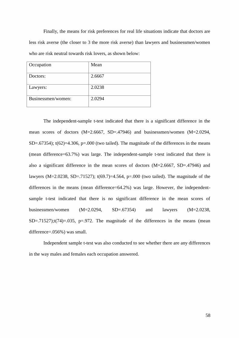
58
Finally, the means for risk preferences for real life situations indicate that doctors are
less risk averse (the closer to 3 the more risk averse) than lawyers and businessmen/women
who are risk neutral towards risk lovers, as shown below:
Occupation Mean
Doctors: 2.6667
Lawyers: 2.0238
Businessmen/women: 2.0294
The independent-sample t-test indicated that there is a significant difference in the
mean scores of doctors (M=2.6667, SD=.47946) and businessmen/women (M=2.0294,
SD=.67354); t(62)=4.306, p=.000 (two tailed). The magnitude of the differences in the means
(mean difference=63.7%) was large. The independent-sample t-test indicated that there is
also a significant difference in the mean scores of doctors (M=2.6667, SD=.47946) and
lawyers (M=2.0238, SD=.71527); t(69.7)=4.564, p=.000 (two tailed). The magnitude of the
differences in the means (mean difference=64.2%) was large. However, the independent-
sample t-test indicated that there is no significant difference in the mean scores of
businessmen/women (M=2.0294, SD=.67354) and lawyers (M=2.0238,
SD=.71527);t(74)=.035, p=.972. The magnitude of the differences in the means (mean
difference=.056%) was small.
Independent sample t-test was also conducted to see whether there are any differences
in the way males and females each occupation answered.

59
Businessmen/women:
An independent sample t-test was initially conducted to compare the way in which
businessmen and businesswomen acknowledged their risk preferences. There was no
significant difference in scores for businessmen (M 2.5294, SD=1.32842) and
businesswomen (M=3.2353, SD=1.20049); t(32)=-1.625, p=.114 (two tailed). The magnitude
of the differences in the means (mean difference=-70.5%) was small.
The independent sample t-test was also conducted to compare the way in which
businessmen and businesswomen feel once at risk. There was no significant difference in the
mean scores of businessmen (M=2.8824, SD=.99262) and businesswomen (M=3.4706,
SD=.79982); t(32)=-1.903, p=.066 (two tailed). The magnitude of the differences in the
means (mean difference =.58.8%) was small.
The independent sample t-test was conducted to compare businessmen and
businesswomen willingness to pay to play a gamble. The test indicated that there was no
significant difference in the mean scores for businessmen (M=2.1429, SD=.864444) and
businesswomen (M=2.0000, SD=.93541); t(29)=.438, p=.665 (two tailed). The magnitude of
the differences in the means (mean difference=.14.2%) was small.
The independent sample t-test was also conducted to compare businessmen and
businesswomen willingness to accept in order not to play the gamble indicated that there was
no significant differences in the mean score of businessmen (M=2.7143, SD=.61125) and
businesswomen (M=2.6471, SD=.60634); t(32)=.306, p=.792 (two tailed). The magnitude of
the differences in the means (mean difference=.06.7%) was small.
An independent sample t-test was also conducted to see whether there were any
differences between the risk preferences in real life of businessmen and businesswomen. The
test indicated that there is no significant relationship between the mean scores of males

60
(M=2.0599, SD=.65565) and females (M=2.0000, SD=.70711); t(32)=.223, p=.251 (two
tailed). The magnitude of differences in the means (mean differences=-.05.8%) was small.
Lawyers:
An independent-sample t-test was conducted to compare the way in which male and
female lawyers acknowledge their risk preferences to be. The independent sample t-test
indicated that there is no difference between the scores for male (M=2.7500, SD=.4426) and
female (M=3.0909, SD=.97145); t(40)=-1.437, p=.158 (two tailed). The magnitude of
differences in means (mean difference=-34.0%) was small.
An independent sample t-test was conducted to compare the way in which male and
female lawyers feel once at risk. The test indicated that there is no significant difference in
the mean scores of male (M=2.600, SD=.50267) and female (M=2.4545, SD=1.18431);
t(28.8)=.536, p=.603 (two tailed). The magnitude of differences in the means (mean
difference=.14.5%) was small.
The independent sample t-test was conducted to compare male and female lawyers
willingness to pay to play a gamble. The test indicated that there was no significant difference
in the mean scores for males (M=1.4000, SD=.75394) and females (M=1.5000, SD=82717);
t(37.6)=-.400, p=.692 (two tailed). The magnitude of differences in the means (mean
difference=-.10.0%) was small.
The independent sample t-test was also conducted to compare male and female
lawyers willingness to accept in order not to play a gamble indicated that there was no
significant difference in the mean scores of males (M=2.7000, SD=.57124) and females
(M=2.3684, SD=.76089); t(37)=1.544, p=.131 (two tailed). The magnitude of differences in
the means (mean difference=.33.1%) was small.

61
An independent sample t-test was also conducted to see whether there were any
differences between the risk preferences in real life of male and female lawyers. The test
indicated that there is no significant relationship between the mean scores of males
(M=2.0500, SD=.75915) and females (M=2.0000, SD=.69007); t(38.5)=.223, p=.825 (two
tailed). The magnitude of differences in the means (mean differences=-.05.0%) was small.
Doctors:
An independent-sample t-test was conducted to compare the way in which male and
female doctors acknowledge their risk preferences to be. The test indicated that there is a
significant difference in the mean scores of males (M=2.7059, SD=.91956) and females
(M=3.4667, SD=1.06010); t(30)=-2.175, p=0.38 (two tailed). The magnitude of differences
in the means (mean difference=-.07.6%) was large.
An independent-sample t-test was conducted to compare the way in which male and
female doctors feel once at risk. The test indicated that there is a significant difference
between the mean scores for males (M=3.1176, SD=.60025) and females (M=4.0000,
SD=.84515); t(30)=-3.436, p=.002 (two tailed). The magnitude of differences in the means
(mean difference=-.08.8%) was large.
The independent sample t-test was conducted to compare male and female doctors
willingness to pay to play a gamble. The test indicated that there was no significant difference
in the mean scores for males (M=1.5882, SD=.87026) and females (M=1.2667, SD=.59362);
t(28.3)=1.233, p=.228 (two tailed). The magnitude of differences in the means (mean
difference=.32.1%) was small.
The independent sample t-test was also conducted to compare male and female
doctors willingness to accept in order not to play a gamble indicated that there was no
significant difference in the mean scores of males (M=2.4706, SD=.87447) and females

62
(M=2.5714, SD=.75093); t(29)=-.339, p=.737 (twp tailed). The magnitude of differences in
the means (mean difference=-.10%) was small.
An independent sample t-test was also conducted to see whether there were any
differences between the risk preferences in real life of male and female doctors. The test
indicated that there is no significant relationship between the mean scores of males
(M=2.5625, SD=.51235) and females (M=2.7857, SD=.42582); t(27.9)==1.303, p=.203 (two
tailed). The magnitude of differences in the means (mean differences=-.22.3%) was small.
Chi-Square tests:
Chi-square tests were also conducted to see whether there is a relationship between
individuals risk preferences in hypothetical and neither real life situations. The Pearson Chi-
square test indicated that there is no association for willingness to pay and individuals risk
preferences in real life (Pearson chi-square significance value is .063); neither for willingness
to accept and individuals risk preferences in real life (Pearson chi-square significance value is
.065). Specifically, for doctors the Pearson chi square significance value for Q6WTP and Q9
is .274 and for Q6WTA and Q9 is .329. For businessmen/women the Pearson chi square
significance value for Q6WTP and Q9 is .490 and for Q6WTA and Q9 is .564). And for
lawyers the Pearson chi square significance value for Q6WTP and Q9 is .274 and for
Q6WTA and Q9 is .329.
Chi-square tests for independence were conducted to see whether there is an
association between the way individuals in each occupation perceived their risk preferences
to be and how they were in hypothetical and real life situation. For doctors there was no
association between their perceived risk preferences and risk preferences in hypothetical
gamble situations. The Pearson chi square significance value for Q4 and Q6WTP was .390,
and the Pearson chi square significance value for Q4 and Q6WTA was .790. There was no

63
association between the way doctors perceived their risk preferences to be and their risk
preferences in real life situation, as the Pearson chi square significance value was .902.
For businessmen/women there as for doctors there was no association between their
perceived risk preferences and risk preferences in hypothetical gamble situations. The
Pearson chi square significance value for Q4 and Q6WTP was .397 and the Pearson chi
square significance value for Q4 and Q6WTA was .116. There was no association between
the way businessmen/women perceived their risk preferences to be and their risk preferences
in real life situation, as the Pearson chi square significance value was .712.
However, for lawyers there was an association between their perceived risk
preferences and risk preferences in hypothetical gamble situations for willingness to pay, as
the Pearson chi square significance value was .005. However, there was no association
between the way lawyers perceived their risk preferences to be and their risk preferences for
willingness to accept was .759. There was no association between the way lawyers perceived
their risk preferences to be and their risk preferences in real life situation, as the Pearson chi
square significance value was.562.
Regression Analysis:
Finally, multiple regressions were used. ‘Multiple regressions can be used to explore
the interrelationship among a set of variables (between one continuous dependent variable
and a number of independent variables). Multiple regression can also indicate how well a set
of variables is able to predict a particular outcome, it also provides information about the
model as a whole and the relative contribution of each of the variable that make up the model
and allows testing whether adding a variable contributes to the predictive ability of the
model, over and above those variables already included. Additionally multiple regression can

64
statistically control for an additional variable when exploring the predictive ability of the
model’ (Pallant, 2007:146).
Regression analysis was conducted to explore the interrelationship between gender,
age and occupation and willingness to pay to play a hypothetical gamble. Regression analysis
indicated that 12.2% of willingness to pay to play a hypothetical gamble was explained by
gender, age and occupation. The rest 88.8% of the variance was explained by other variables
that remain unexplained (not measured in this case). The f-statistic of 2.226 and significance
of .047 implies that Ho: there is no relationship between gender, age and occupation and
willingness to pay to play a hypothetical gamble, is rejected. Specifically,
businessmen/women are willing to pay more to play a hypothetical gamble than lawyers and
doctors. This finding is statistically significant (where p‹0.05 as the value is .003). The
regression analysis indicated that there is no significant difference between gender and age
and these variables to do not affect the willingness to pay to play the gamble.
Regression analysis was also conducted to explore the interrelationship between
gender, age and occupation and willingness to accept in order not to play a hypothetical
gamble. Regression analysis indicated that only 5.0% of willingness to pay to play a
hypothetical gamble was explained by gender, age and occupation. The rest 95.0% of the
variance was explained by other variables that remain unexplained (not measured in this
case). The f-statistic of .828 and significance of .551 implies that Ho: there is no relationship
between gender, age and occupation and willingness to accept in order not to play a
hypothetical gamble, is not rejected. Regression analysis indicated that there was no
difference between gender, age or occupation. Furthermore, the regression analysis indicated
that neither gender, age not occupation made a significant contribution to willingness to
accept in order not to play the gamble.

65
Finally, regression analysis was conducted to explore the interrelationship between
gender, age and occupation and risk preferences in real life situation. Regression analysis
indicated that 38% of willingness to pay to play a hypothetical gamble was explained by
gender, age and occupation. The rest 62% of the variance was explained by other variables
that remain unexplained (not measured in this case). The f-statistic of .8580 and significance
of .000 implies that Ho: there is no relationship between gender, age and occupation and risk
preferences in real life situation, is rejected. Specifically, the regression analysis indicated
that doctors are more risk averse than businessmen/women and lawyers. Moreover, there is
no significant difference between genders, age, and occupation; and gender and age are not
significant determinants of risk preferences in real life situations.

66
Chapter five: FINDINGS AND DISCUSSION
5.1 Findings:
The main finding is that Ho: there is no differences between risk preferences among
occupation is rejected; specifically businessmen are less risk averse than doctors and lawyers
for both hypothetical and real life risks. Another finding is that there are no gender and age
differences in risk preferences in hypothetical and real life risk; with the exception of risk
attitudes in real life for businessmen/women indicated that age does affect. Specifically, the
majority of businessmen/women aged 18-25 were risk neutral (83.3%), as well as the
majority of businessmen/women aged 50+ (66.7%). However, businessmen/women aged 26-
35 were risk loving (45.5%) and businessmen/women aged 36-50 were risk averse (36-50%).
Moreover, all three professions acknowledge their risk preferences as when
participants were asked if they enjoy taking risks and being at risks, they gave answers that
reflected their risk attitudes in real life and as well as their attitudes in hypothetical scenarios.
Furthermore, individuals (cross all three professions) risk preferences are not
consistent with their risk preferences in real life.
Finally, the framing effect as suggested by Kahneman and Tversky (1979) holds for
businessmen/women but does not hold for doctors and lawyers.
67
5.2 Discussion:
The fact that businessmen/women appear to be less risk averse than doctors and
lawyers is explained by the fact that they are willing to pay more than the expected value in
order to play a gamble, and prefer to choose the riskier options than the certain option for
financial risks. Moreover, their risk attitude in daily life is more risky compared with doctors
and lawyers.
It can be argued that the finding that businessmen are risk lovers is in line with
previous finding by Hartog, 2002, who studied risk preferences in the Charted Accountants
profession. According to Hartog, 2002 accountants are risk lovers due to the nature of their
profession; specifically as Hartog, 2002 argues ‘it becomes a habit for accountants to value
risky prospects and expected value’ (Hartog, 2002:9). Similarly, Jhonson and Powell (1994)
who study risk preferences of managers argue that, ‘most decisions by managers are made in
environments characterized by uncertainty, judgements often involve subjective assessments
of the uncertain opportunities and threats or costs associated with particular actions. Decision
making is therefore associated with risk taking, balancing potential rewards against the
negative consequences of a particular course of action. High potential rewards are often
associated with large potential losses and consequently the propensity of a manager to seek or
shy away from such high risk options can have serious implications for the organization’
(p123).
Following this line of argument, it can be argued that businessmen/women are risk
lovers as a result of their profession. This is because they are constantly exposed to, and
required to make decisions under uncertainty and risk. Therefore, as ‘conventional wisdom
asserts, the role model of an entrepreneur requires to make risky decisions in uncertain
environments and hence that more risk averse individuals are less likely to become

68
entrepreneurs’ (Caliendo et al, 2006:153). Consequently, one could argue that in order for
businesses to succeed, in other words to ensure high returns it is important for the people that
represent it to be able to take up high risks, as ‘managerial ideology portrays a good manager
as being a risk taker’ (March and Shapira, 1992:1415). However according to Brenne and
Shapira (1983) and Mueller (1969) ‘managers do not believe that risk and return are
positively correlated’ (March and Shapira, 1992:1406).
The fact that this research finds that businessmen/women are risk neutral towards risk
lovers confirms early studies by Cantillon (1755), Marshal (1890) and Knight (1921) who
argue that entrepreneurs are risk bearers. This finding is also in line with the findings by
Caliendo et al (2006), ‘who adopt the German Socio- Economic Panel, which allows the use
of experimentally validated measures of risk attitudes, find that individuals with lower risk
aversion are likely to become entrepreneurs’ (Caliendo, 2006:153).
Moreover, it can be argued that businessmen/women receive appropriate learning
through University as they are taught probability theory and decision making, this therefore
can explain risk preferences of young businessmen/women.
As mentioned in the literature review, risk preferences may be determined prior to
engaging in an occupation. In other words it is not only occupation that determines risk
preferences, but it can work vice versa, that is risk preferences can determine occupation.
Therefore, it can be argued that the fact that businessmen/women are less risk averse can be
explained by referring to Kihlstrom and Laffront (1979) suggestion that ‘running a business
is equivalent to the choice of a risk prospect, the less risk averse will become entrepreneurs
while the relatively risk averse will prefer to be employees and work for a fixed wage’
(Guiso, and Paeilla, 2004:8). Moreover, Kanbur (1979) argue that ‘the degree of risk aversion
is imperative in entrepreneurial decision; and therefore individuals who are more risk seeking

69
tend to chose to become entrepreneurs; compared to more risk averse individuals who choose
employment which offers a fixed salary.
One interpretation of why this dissertation found that doctors and lawyers are risk
neutral towards risk averse could be explained due to the fact that doctors and lawyers learn
through their profession not to take risks as they are constantly faced against choices that
involve human lives which entails that the extent of which they are able to take risks is
limited. They must not make choices based on feelings rather they must be more objective in
their decision making.
Moreover, as suggested by Curtley et al (1986), ‘individuals exhibit risk aversion
when they are assessed by others after they have made a decision and perhaps they anticipate
it will be difficult to convince others that they have made a good decision when the
information available cannot be documented precisely’ (obtained from Kunreuther et al,
1995:347). The fact that the decisions made by doctors and lawyers may be assessed by
others and may be held liable in case of making an ill decision (i.e doctors and lawyers may
be accountable to the patients and clients families), may be a reason explaining their risk
aversness. Moreover taking a decision that may have an adverse effect and may be criticised
by others will most likely haunt their consciousness. Compared to businessmen, where lives
are not at stake, doctors and lawyers’ decision making cannot be affected by context and
environment.
Furthermore, it can be argued that doctors and lawyers may rely on what March and
Shapira (1992) refer to as reference points when making decisions under risk and uncertainty.
That is, doctors and lawyers may regard the probability of failure as being high (over the
reference point that they set) and may consequently result in severe consequences (i.e death
of a patient or imprisonment of a client) and therefore may decide to refrain from taking up
the case. Risk averseness will be heightened when individuals ‘have less knowledge

70
concerning the outcome of a situation and may therefore feel less competent and more
unwilling to bet on the event in question’ (Heath and Tversky, 1991; obtained by March and
Shapira, 1992:248)
It can also be argued that ‘brain sex’ is an important implication in explaining risk
attitudes. The human brain is divided into two hemispheres the left and the right. Evidence
suggests that males use the left brain which is reality based, and requires being logical and
paying attention to detail, while females are right brained which uses feelings, symbols and
languages; and imagination rules (APP: The Daily Telegraph, October, 05, 2007). Evidence
by Govier and Boden (1997) indicate that doctors should have male differentiated brains’
(obtained from Radford, 1998:10) that is, they are required to have logical, and reality based
attributes. Although research by Gower and Bobby (1997) also indicate that ‘lawyers,
accountants, managers and tax inspectors also are left brain dominant as a result of the fact
that these occupation require logical, sequential and analytical skills, this is not always the
case, as individuals in such occupations may use both sides of the brain’ (obtained from
Radford, 1998:9). This therefore may explain why doctors are more risk averse as they are
required to be objective and logical compared to lawyers and businessmen/women who may
be required to interpret symbols and languages; and are often required to perform based on
feelings and instinct.
The framing effect as suggested by Kahneman and Tversky (1979) does not hold for
doctors and lawyers as regardless of the way answers are worded (initially positive and then
negative), both lawyers and doctors chose answers B in both cases for question 8. However
businessmen/women chose answer A in the first case and then chose answer B in the second
case indicating that the way answers are framed affect their decision making under risk and
uncertainty confirming Kahneman and Tversky (1979) findings.

71
The fact that the framing effect as suggested by Kahneman and Tversky (1979) does
not hold for doctors and lawyers can be explained by the fact that doctors and lawyers learn
through their profession to evaluate cases objectively and not based on emotions. This is
especially the case for doctors as their decision involve human lives. Whereas
businessmen/women often make decisions based on instincts and inside information,
something that cannot be made in the case of doctors and lawyers.
The finding that there was no association between the way in which individual
perceive their risk preferences to be and their risk preferences in hypothetical gambling
situations and in actual life indicates that individuals often overestimate their abilities but
when faced with an actual situation other factors, often unconsciously impact their decisions.
This can be explained due to the fact that individuals often view themselves in a positive light
as suggested by Wallach and Wing (1968).
Moreover, the fact that this dissertation found that there is no relationship between
individual risk preferences in hypothetical and real life situation confirms Eckel and
Grossman (2008) argument that risk attitudes vary across environments and contexts; Holt
and Laury (2002) argument that real payoffs impact individual’s risk attitudes and Powell and
Ansic (1997) suggestion that laboratory experiments do not involve real winnings. Moreover
Anderson and Brown (1984) suggestion that motivations are ignored in laboratory
experiments is also confirmed. Along the same lines, another important finding was that
when participants were asked if there is anything else that they would like to add, indicated
that they acknowledged the downsides associated with laboratory experiments mentioned
above, as in particular one respondent (doctor) said that ‘if you ask me the same questions
tomorrow I will give you different answers’. Another respondent (lawyer) admitted that ‘the
context, motives behind a decision, consequences of actions, mood affect risk preferences’.

72
Respondents further acknowledge that they are different types of risk and each
individual values each risk differently. As one respondent (doctor) said ‘there are different
kinds of risk for different kind of people. Some people may risk their lives but may be afraid
to risk their well being and the opposite’. Respondents also acknowledge that risks may often
present opportunities. As one respondent (lawyer) said:’ some risks may lead to something
better, but we must be careful for some risks such as not wearing a seatbelt, smoking’. A
doctor said that ‘marriage and child bearing are two of factors that affect risk attitudes’.
Another interesting finding was that religion and personal ideologies affect
individuals risk preferences. In particular two respondents (both businessmen) refrained from
answering questions 6 and 7 that required that participants chose options in hypothetical
gamble scenarios as a result of religious beliefs and personal ideologies. They argued that
these two factors prevent them from engaging in gambling. This attitude is consistent with
findings by Hartog et al (2002) who find that religion increases risk aversion; more
specifically that risk aversion increases with church attendance. The reasoning that Hartog et
al (2002) provide for this observation is that religious individuals perceive gambling as
reducing their chances of a good afterlife.
Participants throughout all occupations indicated that their willingness to accept a
certain amount in order to stop playing the gamble was higher than the expected value, and
was also much more than the money that they would pay to play the gamble. This finding
confirms previous findings by Horowitz et al (2000) who state that ‘previous authors have
shown that willingness to accept is usually substantially larger than willingness to pay, and
most almost all have remarked that the willingness to pay/willingness to accept ration is
much higher than their economic intuition would predict’ (obtained from Plott and Zeiler,
2005:531). This finding is not only due to misconceptions and confusion as suggested by
Plott and Zeiler (2005), as anonymity was ensured but there were no incentive-compative

73
elicitation mechanism, and subjects did not receive practice and training on the elicitation
mechanism before measuring valuations as was provided by Plott and Zeiler (2005).
Therefore it can be argued that this may be a result of both a degree of misconception of the
methodology of the experiment; but also it is due to human preferences.
It can further be argued that expected value theory is rejected as participants did not
evaluate risky objects by their expected value. Instead participants indicated that they were
willing to spend more than the expected value both for insurance and for gambles (when
asked willingness to accept and willingness to pay). This indicates that the subjective
expected utility is greater than the expected value. This can be explained by the fact that ‘the
utility of insurance is higher than expected value since a loss without insurance may be often
be ruinous’(Warneryd, 1996:750-751); and the same applies for gamble where the ‘utility
appears to be higher as ‘people dream about winning high prices’ (Warneryd, 1996:750-751).
This deviation of actual risky choices from expected value maximization confirms previous
behavioural studies of decision making most carries out in laboratories (Warneyrd, 199).
This findings also confirms the prospect theory which assumes that ‘subjective
decision weights replace probabilities and that loss aversion rather than risk aversion is an
overriding concepts as people pay attention to gains and losses rather than to wealth’
(Warneyrd,1996:751). Furthermore, as mentioned in the literature review, prospect theory
explains that ‘people are risk averse for gains with high probabilities and for losses with low
probabilities and risk seeking for gains with low probabilities and losses with high
probabilities. This pattern is explained by the weighting function for probabilities which
overweights small probabilities and underweights moderate and high probabilities. The
tendency for people to be risk seeking for gains with low probabilities is presumably
enhanced with increasing amounts of money. They will accept low probabilities to win large
prizes in lotteries. The existence of large prizes with low probabilities would be more
74
attractive than the possibilities of winning small prizes with much higher probabilities’
(Warneyrd, 1996:751).
This research found that gender in occupations does not affect risk preferences. This
confirms previous studies by Johnson and Powell (1994) who found that gender differences
in risk preferences exist for non-managerial population, but it does not exist for the
managerial population. This finding also is in line with the findings by Welsh and Young
(1984) and Birley (1989) who found no gender differences in risk preferences of
entrepreneurs. It can be argued that gender differences in occupations is not different due to
the fact that individuals receive the same education. Differences in risk preferences within
occupation could be instead attributed to ‘experience, information access, and personality
types, and age, rather than gender’ (Johnson and Powell, 1994:133). Powell and Ansic (1997)
however find gender differences in managerial population and argues that ‘these differences
are not explained by the context, instance of familiarity, ambiguity or gains and losses
framing, but may be a result of motivation’ (p623).
This research also further found that age in occupation is not a significant predictor of
risk preferences. This finding is in strong contrast with the findings by Bring (1995) and
Jianakoplos and Bernasek (1998) found that age is a significant predictor of risky behaviour.
It is also in contrast to the findings by Harbaigh, Krause, Vesterlund (2002) who found that
adults use subjective weights when evaluating a gamble over a loss. It can be argued that this
finding follows the previous line of argument that individuals according to their risk
preferences self-select themselves into occupations. Therefore neither age, neither gender
affects risk preferences but it is intrinsic motivation as suggested by Johnson and Ainsic
(1997) and personality traits.
75
Chapter six: CONCLUSIONS
This research has attempted to review the literature up to date on individual risk
preferences; the problems associated with the methodology adopted by others to research this
topic have been identified as well as contradiction of findings and interpretations. This
research has further attempted to point out the gaps of previous research. To date, the
literature on occupation and risk preferences has been limited. Therefore, in an attempt to fill
in the existing literature in this area, this research has introduced a new research group,
namely doctors, lawyers and businessmen/women.
The main finding of this research is that risk preferences vary between occupations.
Specifically, businessmen/women are less risk averse compared to doctors and lawyers who
are risk averse. Moreover, this research found that gender and age are not significant
determinants of risk preferences within occupation.
The fact that this research has found that risk preferences of individuals vary
according to their occupation confirms previous research, such as Johnson and Powell (1994)
who find differences in risk preferences amongst managerial population and non-managerial
population.
The fact that businessmen/women are less risk averse than lawyers and doctors can be
explained due to the fact that, ‘most decisions by managers are made in environments
characterized by uncertainty, judgements often involve subjective assessments of the
uncertain opportunities and threats or costs associated with particular actions. Decision
making is therefore associated with risk taking, balancing potential rewards against the
negative consequences of a particular course of action. High potential rewards are often
associated with large potential losses and consequently the propensity of a manager to seek or
shy away from such high risk options can have serious implications for the organization’

76
(Jhonson and Powell 1994:123). Moreover, businessmen/women are more risk loving
because in order for businesses to succeed, in other words to ensure high returns it is
important for the people that represent it to be able to take up high risks, as ‘managerial
ideology portrays a good manager as being a risk taker’ (March and Shapira, 1992:1415).
Whereas doctors and lawyers learn through their profession not to take risks as they
are constantly faced against choices that involve human lives which entails that the extent of
which they are able to take risks is limited. They must not make choices based on feelings
rather they must be more objective in their decision making.
Moreover, it can be argued that it is not occupation that reflects risk preferences but
actual individual risk preferences lead individual to seek occupations that reflects their actual
risk preferences. For example individuals choose to become businessmen/women because it
is a profession that requires individuals to be risk lovers, whereas risk averse individual
choose to become lawyers and doctors because this is required by their occupation.
In addition, the fact that age and gender does not affect risk preferences of
professionals could be due to the fact that risk preferences are determined by intrinsic
motivations and experiences. The finding that gender does not affect risk preferences is also
in line with Johnson and Powell (1994) but is in contrast with the findings of Powell and
Ansic (1997).
Moreover, this dissertation found that the framing effect as suggested by Kahneman
and Tversky (1979) does not hold for doctors and lawyers can be explained due to the fact
that in these profesions that involve human lives, professionals learn not to let their emotions
influence their decisions. This is not the case with businessmen/women who are not faced
with human lives but with money and are often called to base their judgements on feelings
and emotions.

77
The finding that there was no association between the way in which individual
perceive their risk preferences to be and their risk preferences in hypothetical gambling
situations and in actual life indicates that individuals often overestimate their abilities.
Moreover, the fact that this dissertation found that there is no relationship between individual
risk preferences in hypothetical and real life situation confirms Eckel and Grossman (2008)
argument that risk attitudes vary across environments and contexts; Holt and Laury (2002)
argument that real payoffs impact individual’s risk attitudes and Powell and Ansic (1997)
suggestion that laboratory experiments do not involve real winnings. Moreover Anderson and
Brown (1984) suggestion that motivations are ignored in laboratory experiments is also
confirmed.
It is important to know what the risk preferences of each profession are and to
acknowledge that gender and age are not associated with risk preferences amongst
professions in order to avoid stereotypes. That is, young doctors and lawyers and female
businesswomen should not have attached labels as being ‘incapable of doing a good job’.
It is important that stereotypes seize to exist in order for societies to prosper and
advance. In order for this to be achieved there is a need for this information to be transmitted
to individuals and the principal way for this to be achieved is through media and education in
schools. The government, church, schools and societies in general must take have a primary
role to play and must take collective action in order to transmit these ideas.

78
6.2 Limitations of this study and Recommendations for further research:
Looking back at this dissertation I come to realize that there are some drawbacks
associated with this research. To begin with, it can be argued that due to the limited time and
financial resources this dissertation was unable to expand to more geographical areas and
professions in order to understand individuals risk preferences; but instead it focused in the
UK and Cyprus and on Businessmen/women, Lawyers and Doctors, therefore it cannot be
considered as a fair representation of the world. It is therefore suggested that for future
research that the sample size is increased and other that other geographical areas and
professions are also considered.
Moreover this dissertation due to lack of time it was unable to examine further
variables that affect risk preferences such as income, marital status, number of dependents
and religion which could allow to expand the discussion of whether further demographic
variables affect risk preferences. It is therefore suggested that those variables are examined,
especially due to the fact that many respondents when asked if there is anything else to add,
they said that the number of children and marital status affects their risk preferences.
It can be suggested that it would have been interesting to examine risk preferences
across time and examine whether certain scenarios or conditions incurred in the past has
changed or affected participants risk preferences.

79
6.3 Reflections:
Despite the drawbacks discussed above of this dissertation in general I believe that the
findings of this dissertation successfully answered all the research questions and allowed for
better insights to be gained on individuals risk preferences. Moreover, this research project
was able to add to knowledge as many of the findings contradicted some of the previous
literature and thus this dissertation was able to fill in some gaps that existed in previous
literature.
Throughout the completion of this research project I came to develop and improve my
skills a great deal. I learned the importance of timing and planning which are very important
skills for any research and researcher. I believe that I was very well organized throughout my
dissertation which allowed me to finish the dissertation on time and have time to proof read it
to ensure that there are no mistakes such as grammar mistakes.
Time management proved to be very important because this allowed me to properly
deal with problems and issues that arose throughout the completion of this dissertation. For
example, although the one clinic which I initially planned to visit agreed that they would be
able to accommodate me; two weeks before my agreed visit they informed me that
unfortunately they were be unable to do so. The ahead planning allowed enough time to
contact other clinics and arrange the visits.
Total word count: 20,000

80
REFERENCES:
Anderson, G and Brown, R.I.F, (1984), ‘Real and laboratory gambling, sensatiuon-seeking
and arousal’, British Journal of Psychology, 75, oo401-410
Anderson, G and Brown, R.I.F, (1984), ‘Real and laboratory gambling, sensation seeking and
arousal’, British Journal of Psychology, Volume 75, pp 401-410
APP (2007) ‘The right brain Vs left brain’, The Daily Telegraph’, October, 05, 2007 obtained
from: http://www.dailytelegraph.com.au/news/the-right-brain-vs-left-brain/story-e6frev20-
1111114577583 [accessed 09/08/09]
Arrow, K, (1971), Essays in the theory of risk bearing, Markham Publishing Company
Bajtelsmit, Bernasek and Jianakoplos, (1999), ‘Gender differences in defined contribution
pension decisions’ Financial Services Review, volume 8, pp 1-10
Bernstein, Peter,L, (1996), ‘Against the Gods: The remarkable story of risk’, John Wiley and
Sons Inc, USA
Biswanger, H.P, (1980), ‘Attitudes towards risk: experimental measurement in rural India’,
American Journal of Agricultural Economics, pp 395-407
Borsch-Domenech, A and Silvestre, J, (1999), ‘Does risk aversion or attraction depend on
income? An experiment’, Economic Letters, Volume 65, pp 265-273
Brinig, M.F (1995), ‘Does mediation systematically disadvantage women?, William and
Mary Journal of Women and the Law, volume 2, pp 1-34
Brockhaus, R.H, (1980), ‘Risk taking propensity of entrepreneurs’, Journal of Acad.
Management, volume 23, pp 509-520
81
Burgess, J.P, (2006), ‘The ethical transformation of risk’, Presented at Values in Decision
Making on Risk, (VADMOR), Stockholm, 14-18 May
Caliendo, M, Fossen,F.M, Kritikos, A.S, (2006), ‘Risk attitudes of Nascent entrepreneurs:
New evidence from an experimentally validated survey’, Small Business
Economics,Discussion paper 600,German Institute of Economic Research, DIW, Berlin, pp
153-167
Chen, C.R, Steiner, L.T, White, A.M, (2001), ‘Risk taking behaviour and managerial
ownership in the United States life insurance indstry’, Journal of Applied Financial
Economics, Volume 11, pp 165-171
Daruvala, A (2007), ‘Gender, risk and stereotypes’, Journal of Risk and Uncertainty,
Volume 35, pp 265-283
Di Mauro, C and Musumeci, R (2008), ‘Linking risk aversion, type of income and
occupational status’, Preliminary version of IAREP-SABE, World Meeting, Rome, Sept 2-6
Donkers, B, Melenberg, B, VanSoest,A (2001), ‘Estimating risk attitudes using lotteries: A
large sample approach’, Journal of Risk and Uncertainty, Volume 22, number 2, pp 165-195
Eckel, C.C and Grossman, P.J.C, (2008), ‘Men, women and risk aversion, experimental
evidence’,Handbook of Experimental Economics Results, volume1
Fisher, C, (2004), Researching and writing a dissertation, Pearson, London
Friedman, M and Savage, L.J, (1948), The utility analysis of choices involving risk’, Journal
of Political Economy, volume 56, number 4, pp 279-394
Friend and Blume, (1975), ‘The demand for risky assets’, American Economic Review,
pp279-304
Froot, K.A, Scarfstein,D.S, Stein, J.C, (1994), ‘A Framework for Risk Management’,
Harvard Business Review, November/December, pp91-102

82
Greene, (1970) Risk aversion, insurance and the future, Indiana University Press, USA
Guiso, L and Paiella, M (2004), ‘The role of risk aversion in predicting individual behavior’,
obtained from: http://repec.org/esLATM04/up.5136.1082045630.pdf [accessed 1/08/2009]
Hakansson, Nils. H, (1970) Friedman- Savage Utility Functions Consistent with Risk
Aversion, The Quarterly Journal of Economics, volume 83 number 3, pp 472-487
Harbaugh , W.T; Krause K; Vesterlund, L, (2002), ‘Risk attitudes of children and adults:
choices over small and large probability gains and losses’, Experimental Economics, Volume
5, pp53-84
Hartog, J, Ferrer-i-Carbonell, A and Jonker, N, (2002), ‘Linking measured risk aversion to
individual characteristics’ Kyklos, Volume 55, number 1, pp 3-26
Hastrof, A and Isen, M, (1982), ‘Cognitive Social PSyhology, Elsevier, New York
Helliar, C.V (2001), ‘Attitudes of UK managers to risk and uncertainty, Institute of Chartered
Accountants of Scotland’, UK
Hillson and Murray-Webster, (2006-7), yearbook, pp 25-27, obtained from: http:www.risk-
attitude.com/dh_rmw.pdf
Holger et al, (2007), ‘Cross-sectional earnings, risks and occupational sorting: The role of
risk aversion’, Journal of Labour and Economics, volume 14, pp 929-937
Holt , C.A and Laury, S.K, (2002), ‘Risk aversion and incentive effects’, The American
Economic Review, Volume 92, Number 5, pp 1644-1655
Houston, D, ( 1964), ‘Risk, Insurance and Sampling’, The Journal of Risk and Insurance’,
Volume 31, Number 4, pp 511-538

83
ISO/IEC Guide 73, (2002), ‘A risk management standard’ AIRMIC, ALARM, IRM.
http://www.theirm.org/publications/documents/Risk_Management_Standard_030820.pdf
[accessed 01/04/2009]
Jhonson, E.J, and Tversky, A, (1983), ‘Affect, Generalization and the perception of risk’,
Journal of Personality and Social Psychology, Volume 45, pp 20-31
Jianakoplos, N.A and Bernasek, A , (1998), ‘Are women more risk averse?’, Economic
Inquiry, Volume xxxvi, pp 620-630
Johnson, J.E.V and Powell, P.L, (1994), ‘Decision making, risk and gender: Are managers
Different?’British Journal of Management, Volume 5, pp 123-138
Kahneman, D and Tverksy, A, (1991), ‘Loss aversion in riskless choice: A reference
dependent model’, Journal of Economics, Volume 106, number 4, pp 1039-1061
Kahneman, D and Tverky, A, (1984), ‘Choices, values and frames’, Journal of American
Psychologist, volume 39, pp 341-350
Kahneman, D and Tversky, A, (1979), ‘Prospect theory: an analysis of decision under risk’,
Econometrica, Volume 42, number,2, pp 263-292
Kahneman, D and Tversky, A, (1980), ‘The function of reference point in individual and
group decision making’, Organizational Behaviour and Human Decision Processes, Volume
46, issue June, pp 55-76
Karni, E, (2005), ‘Savage’s Subjective Expected Utility Model, Journal of Mathematical
Economics, volume 22, issue 3, pp 325-342
Knight, F.H, (1921), ‘Risk, uncertainty and profit’, Houghton Mifflin Company, Boston
Kumar, R, (2005), ‘Research Methodology’,2nd
edition, Sage Publications, London
84
Kunreuther et al (1992), ‘Ambiguity and underwriter decision processes’, Journal of
Economic Behaviour and Organization, 26, pp 337-352
Levy, M and Levy, H, (2002), ‘Prospect theory: Much ado about nothing?’ Management
Science, Volume 48, Number 10, pp 1334-1349
March, J and Shapira, Z, (1987), ‘Managerial perspectives on risk and risk taking’, Journal of
Management Science, Volume 33, number 11, pp 1404-1418
Pallant, J, (2007), ‘SPSS: Survival manual’, 3rd
edition, Open University Press, USA
Pfeffer, L ( 1956), ‘Insurance, its theory and practice in the United States’ 1st edition,
MacGraw Hill, New York
Pfiffelmann, M, (2007), ‘How to solve the St Petersburg Paradox in rank-dependent models?’
Laboratorie de Reserche en Gestion et Economie, ULP, Papier no 91
Plott, C.R and Zeiler, K, (2005) ‘Willigness to pay – willingness to accept gaps and
experimental procedure’,The American Economic Review, volume 93, number 3,pp 530- 545
Powell and Ansic, (1997), ‘Gender differences in risk behaviour in financial decision making:
An experimental analysis’, Journal of Economic Psychology, 18, pp 605-628
Powell, M and Ansic, D, (1997), ‘Gender differences in risk behaviour in financial decision-
making: An experimental analysis’ Journal of Economic Psychology, Volume 18, pp 605-628
Pratt, J.W, (1964), ‘Risk aversion in the small and in the large, Econometrica, volume 32,
issue 1, pp 122-136
Radford, J, (1998), ‘Gender and choices in education and occupation’ Routledge, London
Rieger, M.O and Wang, M, (2006), ‘Cumulative prospect theory and the St Petersburg
Paradox’ Economic Theory, Volume 28, pp 665-679

85
Rohrmann, B, (2004), ‘Risk Attitude Scales: Concepts and Questionnaires, Project Report,
University of Melbourne/Australia - August 2004 obtained from
www.psych.unimelb.edu.au/staff/rohrmann.html [accessed 12/07/09]
Schubert, R, Brown, M, Gysler, M, Brachinger, H.W, (1999), ‘Financial decision-making:
Are women really more risk averse?’, AEA Papers and Proceedings, Volume 82, Number 2,
pp 381-385
Simone, F,I, (2008)‘ Behavioral Finance’, Research Starters Business, p1-13
Sunden, A.E and Surette, B.J, (1998), ‘Gender differences in the allocation of assets in
retirement savings plans’, AEA Papers and proceedings, Volume 88, Number 2, pp 207-211
Sudman, S and Bradburn, N.M, (1986), ‘Asking questions: A practical huide to questionnaire
design’, Jossey-Bass Inc, California
Trimpop, (1994), ‘The psychology of risk taking behaviour’,107 Advances in Psychology,
North Holand
Turner, B. (1994), ‘Causes of Disaster: Sloppy Management’, British Journal of
Management, Volume 5 (3, September), pp 215-219
Wallash, M.A and Wing, C.W, (1968), ‘Is risk a value?, Journal of Personality and Social
Psychology, volume 9, pp 101-106
Warneyd Karl-Erik (1996), ‘Risk attitudes and risky behaviour’, Journal of Economic
Psychology, Volume 17, pp 749-770
Weinstein, N.D, (1980), ‘Unrealistic optimism about future life events’, Journal of
Personality and Social Psychology, Volume 39, pp 806-820
Yaari, R and Young, A.L (1965), ‘Convexity in the theory of choice under risk’ The
Quarterly Journal of Economics, Volume 79, pp 278-289

86
Unknown author, ‘What is risk?
Obtained from: http://pages.stern.nyu.edu/~adamodar/pdfiles/valrisk/ch1.pdf [accessed
01/08/09]

87
Appendix 1: Questionnaire:
I would like to thank you for your participation and time in answering this
questionnaire which is for the dissertation that I am completing as partial fulfilment of
my Masters degree in MA Risk Management at the University of Nottingham. The aim
of this questionnaire is to understand different individual’s attitudes towards risk.
Please note that this questionnaire is anonymous and the answers that you provide will
remain confidential; I would therefore like to ask that you answer these questions as
honestly as possible bearing in mind that there is no right or wrong answer. Please also
note that this questionnaire is researching a sensitive topic therefore it is not a
requirement to answer any question that you do not want or find is personal. The
questionnaire will begin in the following page.

88
1) Please indicate your gender:
Male Female
2) Please indicate your age:
18-25 26- 35 36 – 50 50+
3) Would you say that you:
Enjoy taking risks
Quite like taking risks
Do not mind taking risks
Prefer not to take risks
Do not like taking risks
4) Would you say that you enjoy being at risk?
Always Often Sometimes Rarely Never

89
5) Suppose there is a bag that contains 100 balls, some of which are white and some of
which are black, if you are given the option to play; you win £100 if the ball you draw is
white and £0 if the ball that you draw is black. Which of the following options would you
choose from if:
45% of the balls are white: Play or get £50 for sure
51% of the balls are white: Play or get £50 for sure
Please state the maximum amount of money you are willing to pay to play the lottery if the
proportion of white balls is as follows:
10% £....
30% £....
50% £....
70% £....
90% £....
Please state the maximum amount of money you are willing to accept in order not to play
the lottery if the proportion of white balls is as follows:
10% £....
30% £......
50% £......
70% £....
90% £...
6) Suppose that we toss a coin. Please chose between the following two options:
1) Receive £100 with either heads or tails
2) Receive £200 with heads and £0 with tails

90
7) Suppose that you must choose between two policies to combat a disease that is expected
to kill 600 people. Which of the following two options would you choose from?
A) 200 people will be saved
B) 1/3 probability that 600 people will be saved and 2/3 probability that no one will be
saved
Now suppose that for the same problem you are given other two options to choose
from. Which one would you choose?
C) 400 people will die
D) 1/3 probability that no one dies and 2/3 probability that 600 people will die
8) Have you or would you engage in any of these activities?
YES MAYBE SOMETIMES NEVER
Bungee jumping
Play at the
casino
Exercise
Buy insurance
Wear seatbelt
Smoke
Drive over the
limit indicated
9) Is there anything else that you would like to add?
THANK YOU!
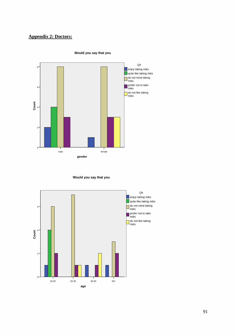
91
Appendix 2: Doctors:
femalemale
gender
8
6
4
2
0
Co
un
t
Would you say that you
do not like taking
risks
prefer not to take
risks
do not mind taking
risks
quite like taking risks
enjoy taking risks
Q4
50+36-5026-3518-25
age
6
4
2
0
Co
un
t
Would you say that you
do not like taking
risks
prefer not to take
risks
do not mind taking
risks
quite like taking risks
enjoy taking risks
Q4
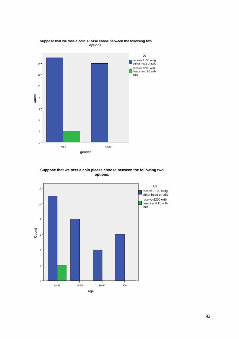
92
femalemale
gender
14
12
10
8
6
4
2
0
Co
un
t
Suppose that we toss a coin. Please chose between the following two
options:
receive £200 with
heads and £0 with
tails
receive £100 wutg
either head or tails
Q7
50+36-5026-3518-25
age
12
10
8
6
4
2
0
Co
un
t
Suppose that we toss a coin please choose between the following two
options:
receive £200 with
heads and £0 with
tails
receive £100 wutg
either head or tails
Q7

93
50+36-5026-3518-25
age
12
10
8
6
4
2
0
Co
un
t
Suppose that we toss a coin please choose between the following two
options:
receive £200 with
heads and £0 with
tails
receive £100 wutg
either head or tails
Q7
femalemale
gender
12
10
8
6
4
2
0
Co
un
t
Suppose that you must chose between two policies to combat a disease that
is expected to kill 600 people. Which of the following two option would you
chose from?
1/3 probability that
600 people will be
saved and 2/3
probability that no
one will be saved
200 people will be
saved
Q8a

94
All doctors chose option B
50+36-5026-3518-25
age
10
8
6
4
2
0
Co
un
t
Suppose that you must choose between two choose between two policies to
combat a disease that is expected to kill 800 people. Which of the following
two options would you choose from?
1/3 probability that
600 people will be
saved and 2/3
probability that no
one will be saved
200 people will be
saved
Q8a
femalemale
gender
20
15
10
5
0
Co
un
t
Suppose that for the same problem as Q8a you are given other two options to
choose from which one would you choose?

95
50+36-5026-3518-25
age
6
4
2
0
Co
un
t
Have you or would you (in the future) do bungee jumping?
never
maybe
Q9a
femalemale
gender
12
10
8
6
4
2
0
Co
un
t
Do you or would you (in the future) engage in bungee jumping?
never
maybe
Q9a

96
femalemale
gender
12
10
8
6
4
2
0
Co
un
t
Do you or would you (in the future) engage in bungee jumping?
never
maybe
Q9a
femalemale
gender
6
4
2
0
Co
un
t
Do you or would you (in the future) play at the casino?
never
sometimes
maybe
yes
Q9b
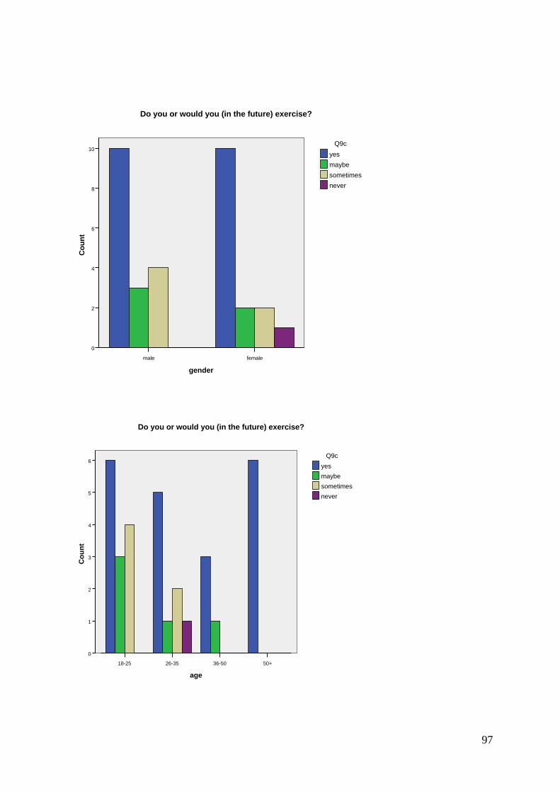
97
femalemale
gender
10
8
6
4
2
0
Co
un
t
Do you or would you (in the future) exercise?
never
sometimes
maybe
yes
Q9c
50+36-5026-3518-25
age
6
5
4
3
2
1
0
Co
un
t
Do you or would you (in the future) exercise?
never
sometimes
maybe
yes
Q9c

98
femalemale
gender
20
15
10
5
0
Co
un
t
Do you or would you (in the future) buy insurance?
sometimes
maybe
yes
Q9d
50+36-5026-3518-25
age
12
10
8
6
4
2
0
Co
un
t
Do you or would you (in the future) buy insurance?
sometimes
maybe
yes
Q9d
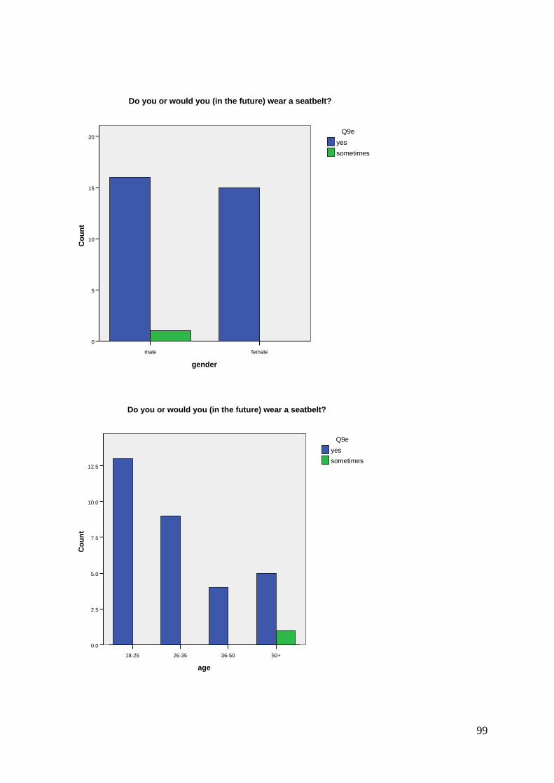
99
femalemale
gender
20
15
10
5
0
Co
un
t
Do you or would you (in the future) wear a seatbelt?
sometimes
yes
Q9e
50+36-5026-3518-25
age
12.5
10.0
7.5
5.0
2.5
0.0
Co
un
t
Do you or would you (in the future) wear a seatbelt?
sometimes
yes
Q9e

100
femalemale
gender
8
6
4
2
0
Co
un
t
Do you or would you (in the future) smoke?
never
sometimes
yes
Q9f
50+36-5026-3518-25
age
6
4
2
0
Co
un
t
Do you or would you (in the future) smoke?
never
sometimes
yes
Q9f
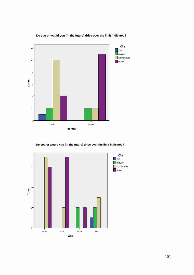
101
femalemale
gender
12
10
8
6
4
2
0
Co
un
t
Do you or would you (in the future) drive over the limit indicated?
never
sometimes
maybe
yes
Q9g
50+36-5026-3518-25
age
6
4
2
0
Co
un
t
Do you or would you (in the future) drive over the limit indicated?
never
sometimes
maybe
yes
Q9g

102
Point 2 is the expected value.
3.503.002.502.001.501.000.50
Q6WTP
25
20
15
10
5
0
Fre
qu
en
cy
do
cto
rs
occu
patio
n
3.503.002.502.001.501.000.50
Q6WTA
25
20
15
10
5
0
Fre
qu
en
cy
do
cto
rs
occu
patio
n

103
Appendix 3: Graphs- Lawyers:
femalemale
gender
14
12
10
8
6
4
2
0
Co
un
t
Would you say that you
do not like taking
risks
prefer not to take
risks
do not mind taking
risks
quite like taking risks
enjoy taking risks
Q4
50+36-5026-3518-25
age
10
8
6
4
2
0
Co
un
t
Would you say that you:
do not like taking
risks
prefer not to take
risks
do not mind taking
risks
quite like taking risks
enjoy taking risks
Q4

104
50+36-5026-3518-25
age
10
8
6
4
2
0
Co
un
t
Would you say that you enjoy being at risk?
rarely
sometimes
often
always
Q5
femalemale
gender
20
15
10
5
0
Co
un
t
Suppose that we toss a coin. Please choose between the following two
options:
receive £200 with
heads and £0 with
tails
receive £100 with
either head or tails
Q7

105
50+36-5026-3518-25
age
12
10
8
6
4
2
0
Co
un
t
Suppose that we toss a coin. Please choose between the following two
options:
receive £200 with
heads and £0 with
tails
receive £100 with
either head or tails
Q7
Phdmastersdegreestill a university
student
education
12.5
10.0
7.5
5.0
2.5
0.0
Co
un
t
Suppose that we toss a coin. Please choose between the following two
options:
receive £200 with
heads and £0 with
tails
receive £100 with
either head or tails
Q7
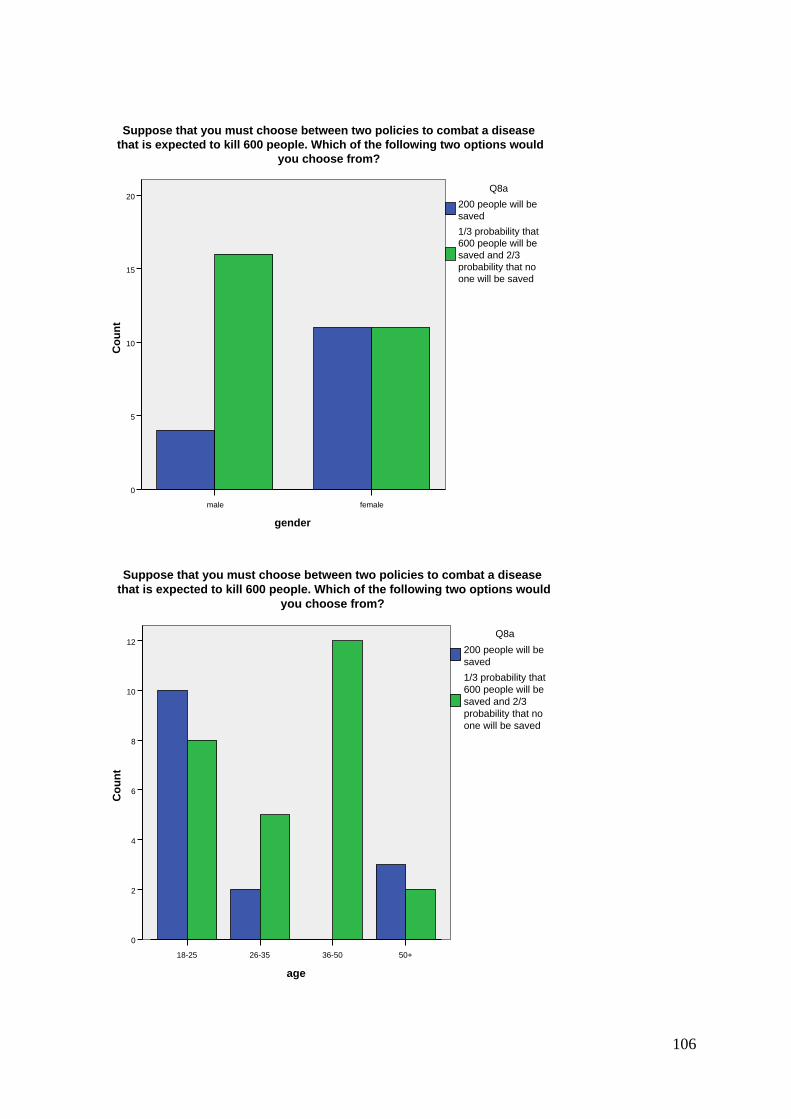
106
femalemale
gender
20
15
10
5
0
Co
un
t
Suppose that you must choose between two policies to combat a disease
that is expected to kill 600 people. Which of the following two options would
you choose from?
1/3 probability that
600 people will be
saved and 2/3
probability that no
one will be saved
200 people will be
saved
Q8a
50+36-5026-3518-25
age
12
10
8
6
4
2
0
Co
un
t
Suppose that you must choose between two policies to combat a disease
that is expected to kill 600 people. Which of the following two options would
you choose from?
1/3 probability that
600 people will be
saved and 2/3
probability that no
one will be saved
200 people will be
saved
Q8a

107
femalemale
gender
14
12
10
8
6
4
2
0
Co
un
t
Suppose that for the same problem as Q8b you are given other two options to
choose from. Which one would you choose?
4.00
1/3 probability that
600 people will be
saved and 2/3
probability that no
one will be saved
400 people will die
Q8b
50+36-5026-3518-25
age
12
10
8
6
4
2
0
Co
un
t
Suppose that for the same problem as Q8b you are given other two options to
choose from. Which one would you choose?
4.00
1/3 probability that
600 people will be
saved and 2/3
probability that no
one will be saved
400 people will die
Q8b

108
femalemale
gender
10
8
6
4
2
0
Co
un
t
Have you or would you (in the future) engage in bungee jumping?
never
maybe
yes
Q9a
50+36-5026-3518-25
age
10
8
6
4
2
0
Co
un
t
Have you or would you (in the future) engage in bungee jumping?
never
maybe
yes
Q9a

109
femalemale
gender
10
8
6
4
2
0
Co
un
t
Do you or would you (in the future) play at the casino?
never
sometimes
maybe
yes
Q9b
50+36-5026-3518-25
age
10
8
6
4
2
0
Co
un
t
Do you or would you (in the future) play at the casino?
never
sometimes
maybe
yes
Q9b

110
femalemale
gender
12
10
8
6
4
2
0
Co
un
t
Do you or would you (in the future) exercise?
never
sometimes
maybe
yes
Q9c
50+36-5026-3518-25
age
12.5
10.0
7.5
5.0
2.5
0.0
Co
un
t
Do you or would you (in the future) exercise?
never
sometimes
maybe
yes
Q9c

111
femalemale
gender
20
15
10
5
0
Co
un
t
Do you or would you (in the future) buy insurance?
never
maybe
yes
Q9d
50+36-5026-3518-25
age
20
15
10
5
0
Co
un
t
Do you or would you (in the future) buy insurance?
never
maybe
yes
Q9d

112
femalemale
gender
20
15
10
5
0
Co
un
t
Do you or would you (in the future) wear a seatbelt?
never
sometimes
yes
Q9e
50+36-5026-3518-25
age
14
12
10
8
6
4
2
0
Co
un
t
Do you or would you (in the future) wear a seatbelt?
never
sometimes
yes
Q9e
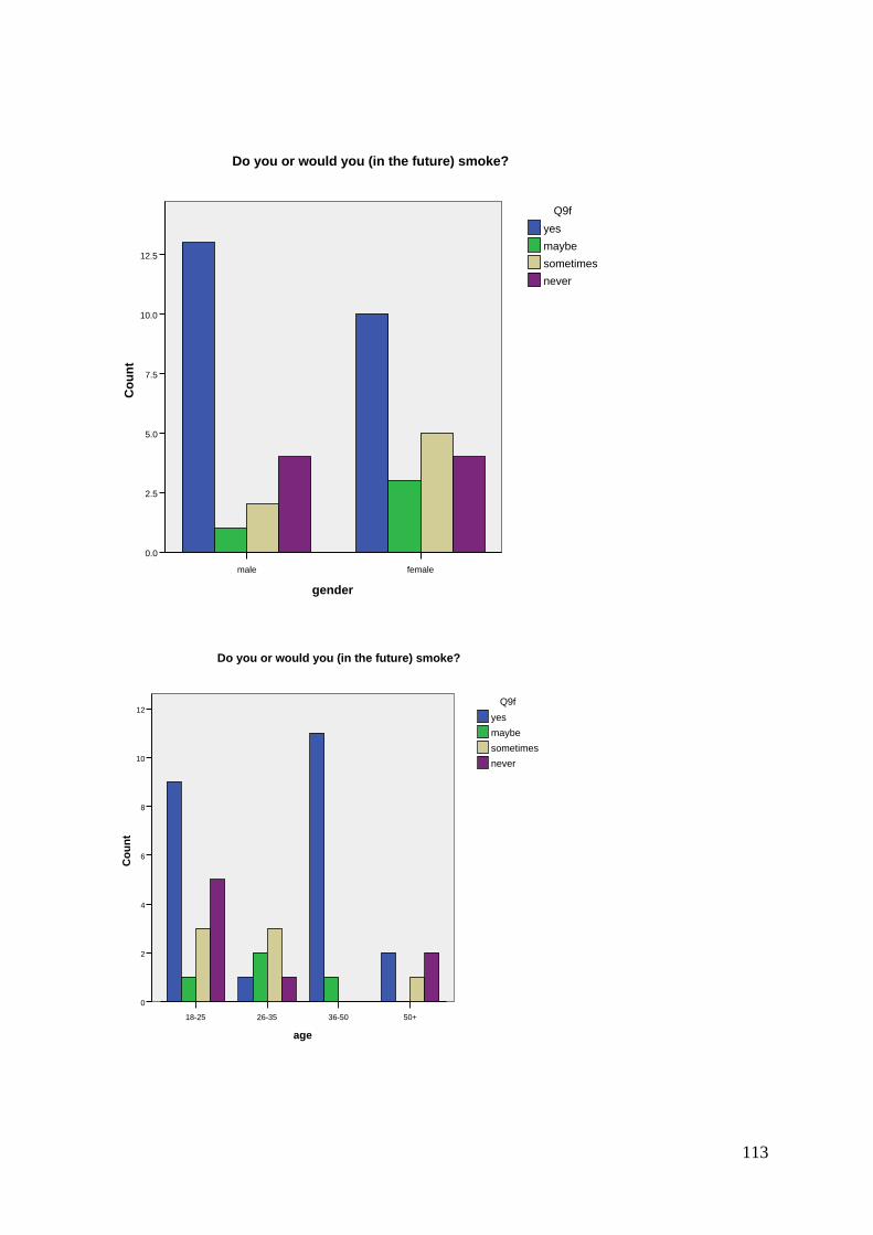
113
femalemale
gender
12.5
10.0
7.5
5.0
2.5
0.0
Co
un
t
Do you or would you (in the future) smoke?
never
sometimes
maybe
yes
Q9f
50+36-5026-3518-25
age
12
10
8
6
4
2
0
Co
un
t
Do you or would you (in the future) smoke?
never
sometimes
maybe
yes
Q9f

114
femalemale
gender
12
10
8
6
4
2
0
Co
un
t
Do you or would you (in the future) drive over the limit indicated?
sometimes
maybe
yes
Qfg
50+36-5026-3518-25
age
10
8
6
4
2
0
Co
un
t
Do you or would you (in the future) drive over the limit indicated?
sometimes
maybe
yes
Q9g

115
Point 2 is the expected value.
3.503.002.502.001.501.000.50
Q6WTP
30
25
20
15
10
5
0
Fre
qu
en
cy
law
ye
rs
oc
cu
pa
tion
3.503.002.502.001.501.000.50
Q6WTA
25
20
15
10
5
0
Fre
qu
en
cy
law
ye
rs
oc
cu
pa
tion

116
Appendix 4: Businessmen/women:
femalemale
gender
5
4
3
2
1
0
Co
un
t
Would you say that you
do not like taking
risks
prefer not to take
risks
do not mind taking
risks
quite like taking risks
enjoy taking risks
Q4
50+36-5026-3518-25
age
4
3
2
1
0
Co
un
t
Would you say that you:
do not like taking
risks
prefer not to take
risks
do not mind taking
risks
quite like taking risks
enjoy taking risks
Q4

117
femalemale
gender
10
8
6
4
2
0
Co
un
t
Would you say that you enjoy being at risk?
never
rarely
sometimes
often
always
Q5
50+36-5026-3518-25
age
8
6
4
2
0
Co
un
t
Would you say that you enjoy being at risk?
never
rarely
sometimes
often
always
Q5

118
femalemale
gender
10
8
6
4
2
0
Co
un
t
Suppose that we toss a coin. Please choose between the following two
options:
receive £200 with
heads and £0 with
tails
receive £100 with
either head or tails
Q7
50+36-5026-3518-25
age
10
8
6
4
2
0
Co
un
t
Suppose that we toss a coin. Please choose between the following two
options:
receive £200 with
heads and £0 with
tails
receive £100 with
either head or tails
Q7

119
femalemale
gender
12
10
8
6
4
2
0
Co
un
t
Suppose that you must choose between two policies to combat a disease
that is expected to kill 600 people. Which of the following two options would
you choose from?
1/3 probability that
600 people will be
saved and 2/3
probability that no
one will be saved
200 people will be
saved
Q8a
50+36-5026-3518-25
age
8
6
4
2
0
Co
un
t
Suppose that you must choose between two policies to combat a disease
that is expected to kill 600 people. Which of the following two options would
you choose from?
1/3 probability that
600 people will be
saved and 2/3
probability that no
one will be saved
200 people will be
saved
Q8a

120
femalemale
gender
14
12
10
8
6
4
2
0
Co
un
t
Suppose that for the same problem as Q8a you are given other two options to
choose from. Which one would you choose?
1/3 probability that
600 people will be
saved and 2/3
probability that no
one will be saved
400 people will die
Q8b
50+36-5026-3518-25
age
12
10
8
6
4
2
0
Co
un
t
Suppose that for the same problem as Q8a you are given other two options to
choose from. Which one would you choose?
1/3 probability
that600 people will be
saved and 2/3
probability that no
one will be saved
400 people will die
Q8b

121
femalemale
gender
10
8
6
4
2
0
Co
un
t
Do you or would you (in the future) engage in bungee jumping?
never
maybe
yes
Q9a
50+36-5026-3518-25
age
6
4
2
0
Co
un
t
Do you or would you (in the future) engage in bungee jumping?
never
maybe
yes
Q9a
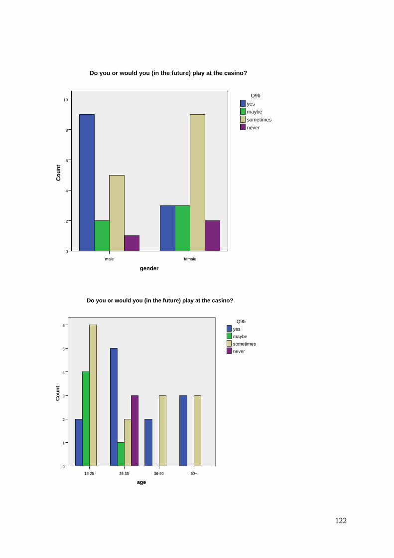
122
femalemale
gender
10
8
6
4
2
0
Co
un
t
Do you or would you (in the future) play at the casino?
never
sometimes
maybe
yes
Q9b
50+36-5026-3518-25
age
6
5
4
3
2
1
0
Co
un
t
Do you or would you (in the future) play at the casino?
never
sometimes
maybe
yes
Q9b

123
femalemale
gender
12.5
10.0
7.5
5.0
2.5
0.0
Co
un
t
Do you or would you (in the future) exercise?
never
sometimes
maybe
yes
Q9c
50+36-5026-3518-25
age
10
8
6
4
2
0
Co
un
t
Do you or would you (in the future) exercise?
never
sometimes
maybe
yes
Q9c

124
femalemale
gender
20
15
10
5
0
Co
un
t
Do you or would you (in the future) buy insurance?
sometimes
maybe
yes
Q9d
50+36-5026-3518-25
age
12
10
8
6
4
2
0
Co
un
t
Do you or would you (in the future) buy insurance?
sometimes
maybe
yes
Q9d

125
femalemale
gender
20
15
10
5
0
Co
un
t
Do you or would you (in the future) wear a seatbelt?
sometimes
yes
Q9e
50+36-5026-3518-25
age
12
10
8
6
4
2
0
Co
un
t
Do you or would you (in the future) wear a seatbelt?
sometimes
yes
Q9e
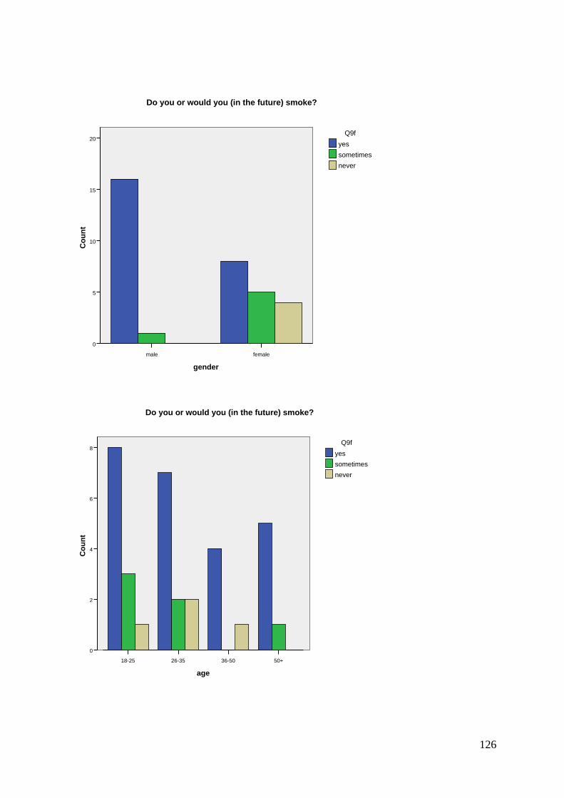
126
femalemale
gender
20
15
10
5
0
Co
un
t
Do you or would you (in the future) smoke?
never
sometimes
yes
Q9f
50+36-5026-3518-25
age
8
6
4
2
0
Co
un
t
Do you or would you (in the future) smoke?
never
sometimes
yes
Q9f

127
femalemale
gender
10
8
6
4
2
0
Co
un
t
Do you or would you (in the future) drive over the limit indicated?
never
sometimes
maybe
yes
Q9g
50+36-5026-3518-25
age
6
4
2
0
Co
un
t
Do you or would you (in the future) drive over the limit indicated?
never
sometimes
maybe
yes
Qfg

128
Point 2 is the expected value.
3.503.002.502.001.501.000.50
Q6WTP
12.5
10.0
7.5
5.0
2.5
0.0
Fre
qu
en
cy
bu
sin
es
sm
en
oc
cu
pa
tion
3.503.002.502.001.501.000.50
Q6WTA
25
20
15
10
5
0
Fre
qu
en
cy
bu
sin
es
sm
en
oc
cu
pa
tion