SERI/TFt-215-1379 December 1981

Atmospheric Effects on Solar Cell Calibration and Evaluation

R. E. Bird R. L. Hulstrom

Printed in the United States of America Ava i 1 able from: National Technical Information Service U.S. Department of Commerce 5285 Port Royal Road Springfield, VA 22161 Price:

Microfiche $3.00 Printed Copy $ 4. 00

NOTICE

This report was prepared as an account of work sponsored by the United States Government. Neither the United States nor the United States Depart~ ment of Energy, nor any of their employees, .nor any of their contractors, subcontractors, or their employees, makes any warranty, express or implied, or assumes any legal liability or responsibility for the accuracy, complete­ness or usefulness of any information, apparatus, product or process disclosed, or represents that its use would·not infringe privately owned rights.

I I I -I I I I I I I I I I I I I I I I

·-,

-,

...)

.....J

--,

_ _J

-,

-,

--,

. .....)

--,

_....J

_ _)

'

·-,

_j

_)

__J

.J

--,

.J

SER:I/TR-215-1379 UC!: Category: 63

Atmospheric E:ffects on Solar c:eH CaUbra!Uon a:nd E:va:lua!Hon

R. E. Bird R. L. Hustrom

December 1981

Prepared under Task No. 1093.00 . WPA No. 116-81

Solar Energy Research Institute A Division of Midwest Research Institute

1617 Cole Boulevard Golden, Colorado 80401

Prepared for the U.S. Department of Energy Contract No. EG-77-C-01-4042

ii

I I

I

11} -fjl

I too

I '

11

I fa I}

I

-,

'

-~

.J

..J

-,

,.,.I

...J

....,

...J

.J

r

J

.J

-,

S::~11:::, ________________________ T_R_-_13_7_9_

PREFACE

This report documents work performed by the Renewable Resource Assessment and Instrumentation Branch of the Solar Energy Research Institute for the U.S. Department of Energy under Task No. 1093.00. It presents results obtained by integrating the point-by-point multiplication of the measured spectral response of a solar cell with a modeled solar spectrum to yield cell calibra­tion numbers and short-circuit currents. We used several modeled spectra and measured cell responses for silicon, gallium arsenide, and cadmium sulfide. The authors would like to thank Bill Kaszeta of SES and Henry Curtis of National Aeronautical and Space Admin-·istration/Lewis for cell response data.

Richard E. Bird

Roland Hulstrom, Chief Renewable Resource and Instrumenta­

tion Branch

Approved for

SOLAR ENERGY RESEARCH INSTITUTE

,-· ; - ,,. / ( __ ) /. ) ,

- -- .'-~~ /<--vu.---;\-1 rt'

Donald Ritchie, Manager Solar Electric Conversion Research

Division

iii

iv

I .

I . .

I I

- . I I .

Ii I

I . il ii

I . . ~ ii

I I . I .

---,

__ _J

··,

.. J

. .,

J

-,

..J

'

. ..,

. ..J

-,

.....J

-,

___J

.......

_J

--,

.--1-f

_J

r

.J

_J

i

_J

55, 1 l•J ________________________ TR_-_1_3_79_

SUMMARY

OBJECTIVES

This report presents results that illustrate atmospheric effects on photovoltaic cell short-circuit currents and cell calibration numbers for silicon, gallium arsenide, and cadmium sulfide. These data illustrate the effects of precipitable water vapor, turbidity, air mass, and global normal irradiance compared with direct normal irradiance on cell performance. It is not the intent of this report to intercompare different cells, but to present results for individual cells separately.

DISCUSSION

The Renewable Resource Assessment and Instrumentation Branch is using solar spectral modeling capabilities that are believed to be more accurate than other models that are widely used in the solar community. As a result, we have taken a new look at the effects of the atmosphere and of global normal irradiance compared with direct normal irradiance on solar cell performance.

CONCLUSIONS

• Rigorous radiative transfer codes are essential for calculating the scattered irradiance component.

• Precipitable water vapor amounts between l to 4 cm caused solar cell calibration number to vary for direct normal radiation by 1. 7% to 4.6% depending on the cell material. All of the cells modeled showed less than a 2% variation except for GaAs, which showed the 4.6% change in cal­ibration number.

• Increases in air mass from 1 to 2 changed cell calibration number for direct normal radiation by 1.0% to 2.6% depending on cell material.

• Increasing turbidity from 0.1 to O. 27 at 500-nm wavelength for direct normal radiation varies the calibration number by 1.4% to 3.1% for vari­ous materials.

• Changing water vapor, air mass, and turbidity simultaneously by the total amounts specified previously varies the cell calibration number for direct normal radiation by the extremes of 4.-5% to 8% for different cells.

• The atmospheric effects on the cell calibration number are much more dif­ficult to predict than those on cell short-circuit current.

• Water vapor has little effect on cell short-circuit current for direct normal radiation when compared with effects of air mass and turbidity.

• Turbidity changes have a small effect on the short-circuit current for global radiation when compared with direct normal radiation •

• The global normal-to-direct normal irradiance ratio should· be less than approximately 1.3 to conform to the reference cell calibration

V

S:t1,.1 __________________________ T_R_-_1_37_9_

specification of the draft ASTM standard that the product of the Angstrom-turbidity coefficient with the air mass be less than 0.25.

• Certain atmospheric conditions exist where global calibration-methods for reference cells have a greater dependency on air mass than do direct nor­mal calibration methods. For cells with spectral responses that cut off below 900 run, such as GaAs and amorphous Si, precipitable water· vapor will greatly affect both global and direct normal calibration methods.

• The GaAs cell analyzed here is significantly more efficient for applica­tions in high water-vapor conditions than in dry conditions.

• The CdS/Cu2S cell analyzed here is much more efficient for flat-plate applications than for concentrator applications under most atmospheric conditions.

vi

r 6..

r L...

r L

r L

r L

r

F

L

--,

-,

--,

' ...I

..J

-,

-,

_ _J

-,

-,

. ..J

• . ...J

--,

, __ _J

..J

, . ..J

..)

. .,

5 -91* TR-1379 =~ I.I

1.0

2.0

3.0

4.0

TABLE OF CONTENTS

Introduction •••••••••••••••••••••••••••••••••••• . . . . . . . . . . . . . . . . . . . . Radiative Transfer Codes •••••••••••••••••••••••••••• . . . . . . . . . . . . . . . . 2.1 2.2 2.3

SOLTR.AN' Code •••••••••••••••••••••••••••••••••••••••••••••••••• • BRITE Code •••••••••••••••••••••••••••••••••••••••••••••••••••• • Other Considerations •••••••••••••••••••••••••••••••••••••••••••

Results ••••••••••••••••••••••••••••••••••••••••••••••• , •••• •••••••••

References •••••••••••••••••••••••••••••••••••••••••• •• •••••• •. • •••• •

vii

1

3

3 4 5

7

19

-

viii

I] .

I ffiW1 il

[11 .

ff! iJ

11 ~ liJ

ffil ~

' .J

-,

..)

.,

'

.,

_...I

---,

-,

- _.J

'

_,,J

-.,

_.J

\

...J

..J

.J

J

TR-1379 sa,1,ll, -------------------------------

2-1

3-1

3-2

3-3

LIST OF FIGURES

Global Spectral Irradiance from Bedford, Mass. (Taken on July 18, 1980; at 12:36 local standard time with spectral features designated.) ••••••••••••••••••••••••••••••••••••••••••••

Photovoltaic Cell Responses (Unknown Active Area) ••••••••••••••••••

N~A Silicon Cell Calibration-3.53 cm2 (SOLTRAN 4-USS Atmosphere-Rural Aerosol) •••••••••••••••••••••••••••••••••••••••••••••••••••

NASA Gallium Arsenide Cell Calibration (SOLTRAN 4-USS Atmosphere-

6

8

8

Rural Aerosol)................................................... 9

3-4 NASA Cadmium Sulfide Cell Calibration (SOLTRAN 4-USS Atmosphere-Rural Aerosol) ••••••••••••••••••••••••••••••••••••••••••••••••••• 9

3-5 SES Silicon Cell Calibration (SOLTRN 4-USS Atmosphere-Rural Aerosol)......................................................... 10

3-6 SES Cadmium Sulfide Cell Calibration (SOLTRAN 4-USS Atmosphere-Rural Aerosol) •••••••••••••••••••••••••••••••••••••••••••••••••••

3-7 SES S_ilicon Cell Short-Circuit Current (SOLTRAN 4-USS Atmosphere-Rural Aerosol) •••••••••••••••••••••••••••••••••••••••••••••••••••

3-8 SES CdS/Cu2S Cell Short-Circuit Current (SOLTRAN 4-USS Atmosphere-.,, Rural Aerosol) •••••••••••••••••••••••••••••••••••••••••••••••••••

3-9 SES Silicon Cell Short Circuit Current (BRITE and SOLTRAN 4 Comparison) ••••••••••••••••••••••••••••••••••••••••••••••••••••••

3-10 SES Silicon Cell Calibration (BRITE and SOLTRAN 4 Comparison) ••••••

3-11 NASA Gallium Arsenide Cell Calibration (BRITE Global and Direct

10

14

14

15

16

Normal Comparison)............................................... 16

3-12 SES CdS/Cu2S Cell Calibration (BRITE and SOLTRAN 4 Comparison)..... 17

LIST OF TABLES

3-1 Modeled Ratio of the Global Normal Irradiance to the Direct Normal Irradiance for Various Air Mass Values and Two Turbidities....... 12

3-2 Approximate Percentage Change in Calibration Number Owing to Changes in Precipitable Water Vapor from 1-4 cm, Air Mass from 1-2, and Turbidity from 0.1-0.27 •••••••••••••••••••••••••••••••••

3-3 Total Irradiance (w/m2) for Modeled Spectral Irradiances •••••••••••

ix

12

13

-

~ ' I

~ '

'

I ; W7 ~

m ~

fEn llib1

En ~

W7} iJ

W) ~

00 '

'

~ f

'

-,

__J

-,

_ _J

-,

_,.)

-,

.J

...I

-.,

_J

·-·'?

_J

-;

-,

_J

--,

...I

.J

.,

.,

)

.J

S:fl ,., ______________________ T_R_-_13_7_9

SECTION 1.0

INTRODUCTION

Early work in solar spectral modeling was performed by Moon (1940). Several spectral models have been produced since Moon's time for use in solar applica­tions. However, because most of these employ the Beer's law approach that Moon used, only minor progress has been made in this field. Most of the improvements have resulted from using more accurate molecular absorption data and improved extraterrestrial solar spectra. These models can accurately pre­dict the direct component of the total solar irradiance, but can provide only rough estimates of the diffuse (scattered) component. The main deficiency of the direct component results is caused by poor quality molecular absorption data.

However, there have been significant advances in radiative transfer modeling for space and military applications. Computer codes have been developed (Lenoble 1977) to solve the equation of radiative transfer much more rigor­ously. In addition, improved molecular absorption data have been generated, but have been overlooked by the solar community. Dave first applied one of these codes and the improved data sets to photovoltaics (1976; 1978a).

The Renewable Resource Assessment and Instrumentation Branch at SERI has taken advantage of these developments and currently has three rigorous codes in operation. One of these, SOLTRAN, is a direct radiation model, and the other two, BRITE and FLASH, are global radiation models.

The next few sections will discuss the SOLTRAN and BRITE codes and their application to solar cell evaluation. The effects of air mass (AM), turbid­! ty, water vapor, and global normal irradiance compared with direct normal irradiance on cell short-circuit current and cell calibration number w~ll be presented for silicon (Si), gallium arsenide (GaAs) and cadmium sulfide cells (CdS). The intent is to examine the atmospheric effects on individual cells and not to intercompare various cells.

1

2

I I I

-I I I I I I I I I I I I I I 11

11

·,

.J

... .,

.. J

J

. ....,

_j

_ _.J

i

.J

.....,

.• ....J

...,

.. --1

.J

. .,

• ..J

....J

_ __J

. .,

J

., )

-, J

1

_J

- TR-1379 sa,1,•, ---------------------------

2. 1 SOLTRAN CODE

SECTIOR 2.0

RADIATIVE TRANSFER CODES

SOLTRAN was constructed from the LOWTRAN (Selby 1975, 1976, 1978; Kneizys 1980) atmospheric transmission code produced by the Air Force Geophysics Lab-. oratory with the extraterrestrial solar spectrum of Thekaekara (1974).

The LOWTRAN code has evolved through a series of updates and continues to be improved with new data and computational capabilities. In this code, a lay­ered atmosphere is constructed between sea level and 100-km altitude by defin­ing atmospheric parameters at 33 levels within the atmosphere. The actual layer heights at which atmospheric parameters are defined are: sea level (O.O km) to 25-km altitude in 1.0-km intervals, 25 to 50 km in 5-km intervals, and at 70 km and 100 km, respectively. At each of these 33 altitudes, the fallowing quantities are defined: temperature, pressure, molecular density, water vapor density, ozone density, and aerosol extinction and absorption coefficients. Mcclatchey described in detail the standard model atmospheres incorporated in this code (1972).

The absorption coefficients of water vapor, ozone, and the combined effects of the uniforml1 mixed gases (co2, N2o, CH4, CO, N2, and o2) ar:

1 stored in the

code at 5-cm 1 wavenumber i!'j_tervals with a resolution of 20 cm • The average transmittance over a 20-cm- interval as a result of molecular absorption is calculated by using a band absorption model, which is based on recent labora­tory measurements complemented by using available theoretical molecular line constants in line-by-line transmittance calculations.

This model includes the effects of earth curvature and atmospheric r~frac­tion. The results of earth curvature become important along paths that are at angles greater than 60 deg. from the zenith; refractive effects then dominate at zenith angles greater than 80 deg •

The scattering and absorption effects of atmospheric aerosols (dust, haze, and other suspended materials) are stored in the code in extinction and absorption coefficients as a function of wavelength. These coefficients were produced by a MIE code for defined particle size distributions and complex indices of refraction. Four aerosol models were available, representing rural, urban, maritime, and tropospheric conditions.

A user can choose any one of six standard atmospheric models incorporated in the code or ~an construct his or her own atmosphere by combining parameters from the standard models or by introducing radiosonde data •

Some of the outputs of the LOWTRAN code include the total transmittance; the transmittance of H2o, o3, and the uniformly mixed gases; and aerosol transmit­tance at each wavelength value specified. In the SOLTRAN code these transmit­tance values are multiplied by Thekaekara' s corresponding extraterrestrial solar irradiance at each wavelength of interest to produce the direct normal

3

S::t11:-:i _________________________ T_R_-_13_7_9

solar irradiance. output.

2.2 BRITE CODE

This code does not include any scattered radiation in its

SERI has two codes that employ the Monte Carlo method: one for a spherical­shell geometry and one for a plane-parallel geometry. Both use deterministic methods to calculate the direct irradiance and statistical methods to calcu­late scattered (diffuse) irradiance.

The Monte Carlo method is a statistical technique of solving the equation of radiative transfer. Probability distributions that characterize both photon scattering and absorption events are sampled randomly. One photon· at a time is followed on its three-dimensional path through the scattering medium. The generation of a photon trajectory is begun by randomly sampling an angle from a probability distribution that describes the spatial distribution of light being emitted from a source. A random length is then drawn from a probability distribution of the distances traveled between successive collisions. Next, a random direction is selected from two angular probability distributions that describe polar and azimuthal scattering, respectively. After a new direction is established, the procedure for choosing a random length and direction is repeated until the desired number of collisions have occurred. At each scat­tering, decisions must be made on the probability of absorption, the probabil­ity of interaction with a molecule or with an aerosol particle, the probabil­ity of absorption at a lower boundary, and the pro ba bili ty of scattering a photon upward from a lower boundary.

The Monte Carlo method has been applied to nuclear and light scattering prob­lems for nearly 20 years. As a ·result, many efficiency techniques have been devised to greatly decrease the computational time required. For example, photon trajectories are never terminated because of absorption; instelild, a statistical weight is associated with each photon and is appropriately adjusted after each collision. The initial value of the weight is unity, and the photon trajectory is terminated only when the weight becomes less than a small predetermined value. Collisions are forced so that photons never leave the atmosphere. The weighting factor associated with the photon is adjusted when a forced collision occurs to remove any bias from the results. The codes described here use the backward Monte Carlo method (Collins 1977), which means that photons are traced backwards from the receiver to the source. This tech­nique is especially useful when a finite receiver and a broad source are modeled. The probability of a photon entering a finite receiver with a restricted field of view (FOV) is very small, and this method forces all pho­tons to enter the receiver.

The two codes that use the Monte Carlo method are called BRITE and FLASH and were developed by Radiation Research Associates, Inc., of Fort Worth, Texas. The BRITE code is for an infinite, plane-parallel atmosphere, and the FLASH code is for a spherical-shell atmosphere. The plane-parallel atmosphere is simpler and more efficient in computer time. However, the plane-parallel geometry loses accuracy as the sun approaches the horizon.

4

r

r L.

F

r

r L...

r L

r L.

r

r

r

L

t;..

r

r

r

L..,

-,

-,

J

-,

J

'

-,

.J

__ )

•• __J

, • ....1

_J

__ ..J

.,

--,

·,

....J

-,

. .J

'

' . .J

-,

...1

$:ti 1.1 ---------------------TR_-_13_7_9

BRITE and FLASH use a multilayered atmosphere within which the scattering and absorption properties can be varied with altitude. Both molecular (Rayleigh) and aerosol (MIE) scattering events can occur, and the scattering functions for each are allowed to vary independently and arbitrarily with altitude. Ground reflection for various albedos is included as an additional type of scattering event. The ground reflection can be assumed to be either lamber­tion, isotropic, or of some arbitrary type. These codes also treat absorption by aerosols, ozone, water vapor, carbon dioxide, oxygen, and other molecular species. An additional feature of these codes is that the polarization. (Stokes parameters) of the scattered light is traced through all orders of scattering. Reflected light from the ground is assumed to be unpolarized and is traced through all orders of scattering.

We built several unique features into these programs that apply to solar prob­lems. Up to 10 wavelengths can be modeled simultaneously in a single computer run. The only assumption is that the aerosol phase function is constant over the wavelength interval being considered, which is a very accurate assumption for relatively narrow wavelength intervals. This capability decreases the computer time by nearly a factor of 10 when data over a broad spectrum, such as the solar spectrum, are desired. We can model up to nine incident angles of the solar radiation in one computer run. In addition, two choices of receiver geometry are available. The first is a conical beam geometry in which the cone about the receiver axis can be divided into a combination of up to 15 polar bins with up to 15 azimuthal bins with!~ ea~r po}fr bin. We can calculate either average spectral radiance (Wm µm sr ) or spectral irradiance (W m - 2 µm -l) for each angular bin together with the total inte­grated value for all bins. The second geometry allows one to calculate spec­tral radiance at point directions on a spherical surface, permitting storage of the data for future use in any receiver geometry desired. A final capabil­ity incorporated for solar application is that of modeling up to six different ground albedos simultaneously.

2.3 OTHER CONSIDERATIONS

We used two aerosol and two atmospheric models to produce the data that will be presented later. Most of the data were generated using the U.S. Standard (USS) Atmospheric Model (Mcclatchey 1972) and the rural aerosol model (Shettle 1975). When SOLTRAN 4 was used, we varied the amount of water vapor from 1.42 cm (the normal USS atmosphere amount) by using the water vapor profiles from other atmospheric models. We simply changed a single input number in the SOLTRAN 4 input data. We varied the turbidity by inputting sea level visibil­ities of 23 km and 250 km, which correspond to turbidities of 0.27 and 0.1, respectively, at 500-nm wavelength. Another atmospheric model used in the BRITE program to produce the 0.1 turbidity data was the Dave model 3 (Dave 1978), which is a Midlatitude Summer (MLS) model with 15 instead of 33 lay­ers. The Dave model 3 uses a different aerosol model than the rural aerosol model •

To aid future discussion, a plot showing where various molecular absorbers are active is shown in Fig. 2-1. These data were taken with the SERI spectroradi­ometer at Bedford, Massachusetts, in July 1980. The spectral resolution of

5

TR-1379 Sifl 1.1 --------------------------------these data is approximately 10 nm, which affects the width and depth of the absorption features.

210 --------------------------------,

180

150

60 \ Fe.Ca(SUN)

o,

500 700 900 1100

Wavelength (nm)

Figure 2-1. Global Spectral Irradiance from Bedford, Mass. (Taken on July 18, 1980; 12:36 local standard time with spectral features designated.)

We used Thekaekara 's extraterrestrial spectrum (Thekaekara 1974) for both SOLTRAN and BRITE for this report. Recent work (Frohlich 1980; Hardrop 1981) has shown that the revised Neckel and Labs (Neckel 1981) spectrum is more accurate than Thekaekara' s. We ·are incorporating Neckel and Labs revised spectrum, but it was not available when this work was performed.

We indicated earlier that the rigorous codes can use layered atmospheric models to simulate the real atmosphere as a function of altitude. However, evidence suggests that the height profiles may not be critical in determining the solar irradiance at the ground surf ace or at the top of the atmosphere (King 1979; Blattner 1980). The height profiles are important at points within the atmosphere. The simple codes that have been employed for solar applications use the total optical depth or an average extinction coefficient rather than extinction coefficients that' vary with altitude. This approximation may be satisfactory for surface calculations.

6

r L.

r

r L

L.

r

r

r

r L

r L

-,

• ..J

' _..J

-,

....J

' _ _J

'

-,

_..J

_..J

_J

..J

_...J

_..J

-,

-'

-,

_ _J

-,

,.J

--,

_J

_J

' .J

s:,1 ,.1 ____________________ TR_-_1_37_9

SECTION 3.0

RESULTS

The analysis performed here uses two parameters to evaluate solar cells: the cell short-circuit current (mA)

Isc = f R(A) S(A) dA 0

and the cell calibration number (mA/mW)

where

I CN = ___ s_c __

CIC)

f S(A) dA 0

R(A) = solar cell spectral response (mA/mW) and

S(A) = solar spectral irradiance (mW/cm2/run).

(3-1)

(3-2)

This analysis is idealized since we have not considered the effect of the cell temperature and the effect of the angle of incidence of the diffuse component of the radiation on the spectral response.

In practice, primary reference cells are produced out-of-doors by measuring the cell short circuit current (numerator in Eq. 3-2) and the total broadband irradiance (denominator in Eq. 3-2). These reference cells are then used to calibrate solar simulators and to calibrate measurements made on .other cells. This whole procedure assumes that the two cells are spectrally matched or that corrections can be made for any differences in their spectral responses. It also assumes that the use of the cell as a reference when calibrating a solar simulator is valid even though the simulator spectrum is probably different than the solar spectrum present for the cell calibration.

The measured spectral responses of the five cells that we consider here are shown in Fig. 3-1. The active area of each of these cells is unknown except for the NASA Si cell, which was 3. 53 cm2• In performing the calcula~ions indicated by Eqs. (3-1) and (3-2), we assumed a cell active area of 1 cm for all except the NASA Si cell, and that the response measurements were made under a one-sun light-bias.

We calculated the calibration number by using Eq. (3-2) for each of the five spectral response curves shown in Fig. 3-1. The SOLTRAN 4 code was used to generate the direct normal terrestrial solar spectrum S(A) for five values of the precipitable water vapor and for two air mass and two turbidity values. The results of these calculations are shown in Figs. 3-2 through 3-6.

We chose the precipitable water vapor and turbidity and air mass values so they would encompass the values currently being proposed as a direct normal

7

• I

555,

1 l•I _____________________ TR_-_13_79

- 0.8

§' E ........ <{

§. Q) U) C: 0 Q. U) Q) a:

0.7

0.6

0.5

0.4

0.3

0.2

0.1

0.0

0.2 0.45 0.7

NASA Si ___ _

NASAGaAs __

NASACdS-·­SESSi ---­

SES CdS/Cu2S---

0.95

Wavelength (µm)

1.2 1.45

Figure 3-1. Photovoltaic Cell Response (Unknown Active Area)

1.7

1.12 ......... --------T--......... --------T----,----~--T---, AM2

Tau (0.5) = 0.1

i 1.10 -+---+----+---+---+-----+~==-""'=+---+----+----1

E .........

i AM2 :- 1.08 -+---f----"7"'~--t------+----=-.....-=::;;...._-+---~=-~Tau (0.5) = 0.27 Q) .0 E :J z

AM1 Tau (0.5) = 0.27

.Q 1.06 -+---+-~--+--:::,~-+---+-----+----t---+----t----t -~

.0

ca CJ 1.04 -+---,,,..._---+-----+----1----+----+----1----+------i

1.02

0.0 0.5 1.0 1.5 2.0 2.5 3.0 3.5 4.0

Water· Vapor (cm)

Figure 3-2. , NASA Silicon Cell Qilibration-3 .53 cm.2

(SOLTRAN 4-USS Atmosphere-Rural Aerosol) 8

4.5

r

L

r

L

r L

r L

L..

r L

......,

. ...I

-,

.J

.., _)

..J

-,

_J

-,

-,

...J

.. ,

. .J

. ..,

_ _J

--,

-,

-,

....J

.J

' . ..J

..,

.J

'"'\

.J

$:~I 1.1 ----------------------T_R-_1_3_79

0.260 -+----+----+-

"'-Q) .c § 0.250 -. l----+-+---"J----+,,,,,.-,:;;.--,,~--1------+-----1-----+------1

z C 0

:;::; <a "'-:e a:s

(.)

~ E

......... <(

E -"'-Q) .c E ::::J z C 0

:;::; <a "'-.c ai (.)

0.240 -+----+r--+-----li----+----1----1---..f------11-----'

,'

0.235

0.0 0.5 1.0 1.5 2.0 2.5 3.0 3.5 4.0 4.5

0.1700

0.1675

0.1650

0.1625

0.1600

0.1575

0.1550

0.1525

0.1500

--

·-

----....

-i-

-i-

-i-

Water Vapor (cm)

Figure 3-3. NASA Gallium Arsenide ~11 Calibration (SOLTR.AN 4-USS Atmosphere-Rural Aerosol)

-

I I AM2 -

Tau (0.5) = 0.1 ----~ --.. -- Tau (

~ i-- -- ---.,,.- -- - __ __,__.----- --~----·--- Tau ( ,,~,-

lo - i--·---· ---·- -------- -_.,...,.....---· 1...,,,,,-,-.•-__.- -------....... -- .-· _ .... i-----.. AM2 /" _.,,.,...--- Tau (0.5) = 0.27-

,,~· ....... ~-/'

,, _.,

I I I I I I I I I

I I I I I I I I I

AM1 0.5) = 0.1 AM1

0.5) = 0.27

0.0 0.5 1.0 1.5 ~.O 2.5 3.0 3.5 4.0 4.5

Water Vapor (cm)

Figure 3-4 •. NASA Cadmium Sulfide Cell Calibration (SOLTR.AN 4-USS Atmosphere-Rural Aerosol)

9

sa,1,•, TR-1379

§' E

......... <(

E -..... Q) .c E :::::J z C 0 ~ ca ..... :9 <U (.)

§' E

......... <(

E -

0.3250

0.3225

0.3200

0.3175

0.3150

0.3125

0.3100

0.3075

0.3050

------- AM2 -'---"'---.L---4---4------+-..,.......,_;:;..+----+Tau (0.5) = 0.27

0.0 0.5 1.0 1.5 .

-.--· AM1

Tau (0.5) = 0.27

AM1 Tau (0.5) = 0.1

2.0 2.5 3.0 3.5 4.0

Water Vapor (cm)

Figure 3-5. SES Silicon Cell Calibration (SOLTRAN 4-USS Atmosphere-Rural Aerosol)

--· .--AM1 Tau (0.5) = 0.27

4.5

0.335--+---,......--t------+----+---+-----11------+----+------+

0.330 ---+---+-+--+----1--+---+--+---+---+-+---t----t-......_--t--+---+-~

0.0 0.5 1.0 1.5 2.0 2.5 3.0 3.5 4.0 4.5

Water Vapor (cm)

Figure 3-6. SES Cadmium Sulfide Cell Calibration· (SOLTRAN 4-USS Atmosphere-Rural Aerosol)

10

(

r

L

r Li

r L...

r b._

r L.

r L,

r

r

W..J

r

r

-,

..I

'

...,

J

1

.J

-,

. ...J

___ .J

. .,

--,

--,

___j

' _ _J

-,

,_;

' . .J

'

_J

' .J

TR-1379

55tl 1• 1----------------

standard for solar reference cell calibrations. The proposed specifications being prepared for the calibration of reference cells at the American Society for Testing and'Materials (ASTM) are:

• Air mass--1 to 2 •

• Water vapor-over 1 cm.

• Direct normal irradiance--over 750 w/m2

• Turbidity--Angstrom turbidity coefficient multiplied by the air mass less than 0.25 or the uncollimated-to-collimated ratio less than 1.2.

For the rural aerosol model that was used for these calculations, the highest turbidity was 0.27, at a 500-nm wavelength. The Angstrom turbidity coeffi­cient was 0.123, which when multiplied by an air mass of 2 results in an Ang­strom turbidity coefficient multiplied by the air mass of 0.246 < 0.25.

It is important to distinguish between turbidity and the angstrom turbidity coefficient. The total optical depth (,;) of a slant path through the atmosphere as measured by a sun photometer is:

(3-3)

where Mis the air mass, A is the wavelength designation of the measurement, 'Ca is the turbidity or aerosol optical depth in a vertical path, ,;R is the Rayleigh scattering a molecular scattering optical depth in a vertical path, and ,;ma is the molecular absorption optical depth in a vertical path. An approximate formula that is used to show the wavelength dependence of the turbidity is given by:

(3-4)

where ~ is the Angstrom turbidity coefficient and ex is a variable that is determined by the aerosol particle size distribution.

Recent calculations of the global normal-to-direct-normal irradiance ratio using the BRITE code are shown in Table 3-1. These results indicate that the global normal-to-direct-normal irradiance ratio should be less than approxi­mately 1.3 to conform to the Angstrom turbidity~ air mass product of less than 0.25.

In comparing Figs. 3-2 through 3-6, one should note that we assumed 1 cm2 of active area for all cells except the NASA Si cell. An examination of these figures reveals that changing precipitable water from 1 to 4 cm, air mass from 1 to 2, and turbidity from 0.1 to 0.27, at 500-nm wavelength, results in the approximate extreme changes in calibration number shown in Table 3-2.

The extremes for the combined effects of water vapor, air mass, and turbidity are between 4.5% and 8%. Under some conditions for a given cell material, an atmospheric parameter change produces little or no change in the calibration number. Examples of this are a change from Ai~l to AM2 for a turbidity of 0.27 for the NASA Si cell and a change from AM! to AM2 for a turbidity of 0.1 for the SES CdS/CuzS cell.

11

TR-1379

55~1,•·-------------------Table 3-1. Modeled Ratio

of the Global Normal Irradi­ance to the Direct Normal Irradiance for Various Air Mass Values and Two Turbidities

AM -c/0.S) GLN/DN

1.0 0.1 1.14 1.0 0.27 1.23 1.25 0.27 1.30 1.5 0.27 1.33 2.0 0.27 1.33

Table 3-2. Approximate Percentage Change in Calibration Number Owing to tbanges in Precipitable Water Vapor from 1-4 cm, Air Mass from 1-2, and Turbidity from 0.1-0.27

Cell Material Precipitable Air Mass Turbidity Water Vapor

NASA Si 2.0 1.7 2.1 NASA GaAs 4.6 1.9 2.9 NASA CdS 1.8 0.95 2.5 SES Si 1.7 2.6 1.4 SES CdS/ Cu2S 2.0 1.7 3.1

A possibly unexpected, although easily understood, result shown in Table 3-2 is the large effect that water vapor has on the calibration number (i.e., efficiency) of GaAs. The spectral response of GaAs illustrated in Fig. 3-1 indicates that very little water vapor absorption occurs within its response limits (see Fig. 2-1). Therefore, as a large change in precipitable water vapor significantly alters the denominator of Eq. 3-2, little change in the numerator dramatically modifies the calibration number. The value of the numerator normally varies in the same direction as the denominator, resulting in a smaller change in calibration number. Because the calibration number is a ratio, it can be difficult to predict the effects seen in Figs. 3-2 through 3-6. One conclusion therefore is. that GaAs is best suited for high water­vapor climates.

The total integrated irradiance for many of the spectra used in this report is shown in Table 3-3. These numbers are useful for calculations that the reader may want to perform.

12

F

L

r L

r· L

r

r L..

r L..

r

r L..

r·

r

r

,..,

_J

..,

-'

-,

__J

-,

...J

1

..J

' • ..J

. ..J

-,

-'

-,

-,

..J

-,

_J

.J

1

...J

S::fl 1., __________________ TR_-_13_7_9

Table 3-3. Total Irradiance (w/m2) for Modeled Spectral Irradiances

AM, ,:a(0.5), H20(cm) Direct Normal Direct Normal Global Normal SOLTRAN 4 BRITE BRITE

1.0, 0.27, 1.42 868.6 854.3 1048.7 1.5, 0.27, 1.42 753.0 737.3 991.2 2.0, 0.27, 1.42 660.6 644.1 859.0 1.0, 0.1, 2.93 948.3 915.1 1040.9 2.0, 0.1, 2.93 790.9 736.7

In contrast to the calibration number, the short-circuit current is very pre­dictable. Two examples of the short-circuit current from the same data set that was used to produce Figs. 3-5 and 3-6 are shown in Figs. 3-7 and 3-8. Figure 3-7 shows the short circuit current of the SES silicon cell for the atmospheric parameters discussed previously. Figure 3-8 is the same type of figure for the SES CdS/Cu2s cell. These figures illustrate that precipitable water vapor has a relatively small effect on the short circuit current, and that air mass and turbidity have relatively large effects under direct normal radiation. These results are expected if one examines terrestrial solar spec­tra that reflect various water vapor, air mass, and turbidity values (Matson 1981).

Figure 3-9 illustrates one example of comparing the effects of global normal and direct normal irradiance on the SES Si cell short-circuit current. Vari­ous combinations of air mass, turbidity, and water vapor are presented here.

The direct normal results from SOLTRAN 4 and BRITE are included in Fig. 3-9. The results from these two codes are slightly different because

• The BRITE code uses a newer set of molecular absorption data than SOLTRAN 4;

• The SOLTRAN 4 code does not calculate the attenuation caused ·by molecular scattering as accurately as the BRITE code in the ultraviolet and visible ends of the spectrum; and

• Different methods and the number of spectral data points used make a lit-tle difference.

A comparison of the BRITE results for the first and the fourth sets of histo­grams ( three histrograms per set) shows that the turbidity has a relatively small effect on the short-circuit current in the global normal mode. The effect of turbidity in the direct normal mode is much larger. We anticipated this result theoretically because all scattered light is lost in the direct mode, whereas approximately 75% of the scattered light is recovered in the global mode. A comparison of the first three sets of histograms shows that a change in air mass has less effect on global normal results than on direct normal results for the same reason as just given for the turbidity.

13

TR-1379

S::~1,•,-----------------

AM2 Tau (0.5) = 0.1

~

34

·32

AM1 ~ 30 Tau (0.5) = 0.1 g

!Q2QQQ2Qf ~ 28 ._ ._

AM1 c3 26 Tau (0.5) = 0.27 ....

W////A -~ 24

AM2 ~ 22 ._ Tau (0.5) = 0.27 _g

r I I 71 en 20

AM2 Tau (0.5) = 0.1

~

18

16

34

32

AM1 ~ 30 Tau (0.5) = 0.1 .§.

!Q2QQQ2Qf ~ 28 ._

AM1 c3 26 Tau(0.5) = 0.27 :=

f7/// (/A ~ 24 c3

AM2 .... 22 ._ Tau (0.5) = 0.27 _g

r 7 7 71 rn 20

18

16

0.42 0.86 1.42 2.93 4.12

Water Vapor (cm)

Figure 3-7. SES Silicon Cell Short-Circuit Current (SOLTR.AN 4-USS Atmosphere-Rural Aerosol)

0.42 0.86 1.42 2.93 4.12

Water Vapor (cm)

Figure 3-8. SES CdS/Cu2S Cell Short-Circuit Current (SOLTRAN 4-USS Atmosphere-Rural Aerosol)

·14

r

L

r

r

L

r

r L

r L.

r

r

r

. .J

-,

-,

. .J

., ...J

"1

-,

..J

. ..,

...,

.. ..,

-,

--,

....I

•

. .....J

-,

.,

..J

!

..J

-,

!

SE~l 11l' BRITE-Global

Normal

I BRITE-Direct

Normal

rzzz, SOLTRAN 4

Direct Normal

t'WV1

34

32

< 30 E --C: 28 (1) "-"-~

26 ()

::: ~ 0 24 "-

c3 - 22 "-0 .c (.I)

20

18

16

TR-1379

1, 0.27, 1.42 · 1.5,0.27,1.42. 2,0.27, 1.42 1,0.1,2.93 2,0.1,2.93

Figure 3-9.

Air Mass, Tau (0.5), H20 (cm)

SES Silicon Cell Short-Circuit Current (BRITE and SOLTRAN 4 Comparison)

Figures 3-10 through 3-12 are histograms, similar to Fig. 3-9, for calibration number rather than for short-circuit current. They illustrate the calibration numbers for Si, GaAs, and CdS/Cu2s, respectively. As we mentioned previously, atmospheric effects on calibration number are less predictable than effects on the short-circuit current.

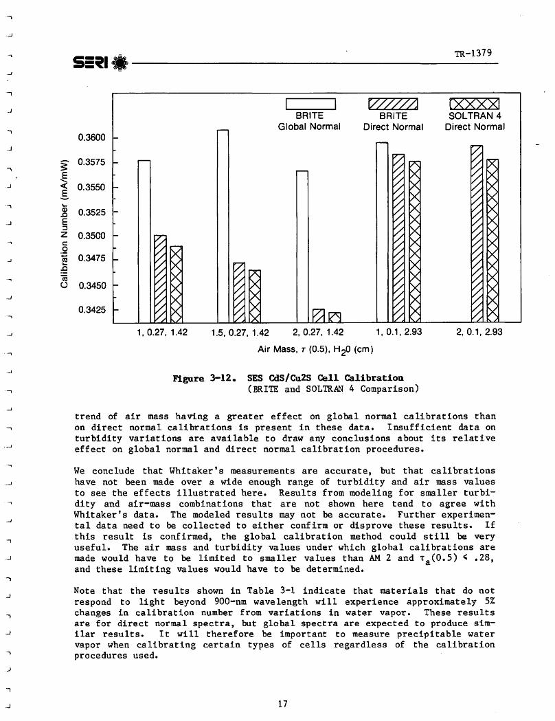
Figure 3-10 shows that at AMl the Si cell is less efficient in the global mode than in the direct' mode. This result reverses for AMl.S and AM2. Figure· 3-12 shows that the CdS/Cu2S cell is always more efficient in the global mode with­in the limits of the atmospheric parameters modeled. In some cases, this cell is significantly more efficient in the global mode. Figure 3-11 for GaAs shows it behaves somewhere between Si and CdS/Cu2S when comparing global and direct radiation performance. CdS/Cu2S uses global radiation more efficiently because it has an enhanced ultraviolet response where scattered radiation dominates.

Recent experimental work (Whitaker 1981) indicates that global normal refer­ence cell calibration methods are less sensitive to air mass and turbidity changes than direct normal calibration procedures. However, an examination of Figs. 3-10 through 3-12 shows that this is not always the case. The results for Si in Fig. 3-10 demonstrates that varying the air mass from 1 to 2 with the turbidity and water vapor remaining constant (i.e., T = 0. 27 and H2o = 1.42 cm) produces a 1.09% change in the direct normal calibration number and a 2.6% change in the global calibration number.

Figure 3-11 shows a similar effect for GaAs. The global results for Ai.~1.5 are believed to be slightly exaggerated (i.e., too large) because of a positive statistical fluctuation in the spectrum near 800-nm wavelength. However, the

15

TR-1379 S:tl,.1 ________________ _

0.3250

0.3225

f 0.3200 ........ <(

.§. 0.3175 ... Q) .0 E 0.3150 :::::, z § 0.3125 :.= ~ :2 0.3100 ca ()

0.3075

0.3050

0.2650

0.2625

f 0.2600 ........ <(

.S 0.2575 ... Q) .0 E 0.2550 :::::, z § 0.2525 :.= ~ :2 0.2500 a

0.2475

0.2450

BRITE Global Normal

1, 0.27, 1.42

BRITE Global Normal

1, 0.27, 1.42

f27/01 BRITE

Direct Normal

1.5, 0.27, 1.42

Rxxx>4 SOL TRAN 4

Direct Normal

2, 0.27, 1.42

Air Mass, r (0.5), H2o (cm)

1, 0.1, 2.93 2, 0.1, 2.93

Figure 3-10. SES Silicon <:ell Calibration (BRITE and SOLTRAN 4 Comparison)

w~ BRITE

Direct Normal

1.5, 0.27, 1.42 2, 0.27, 1.42 1, 0.1, 2.93

Air Mass, r (0.5), H20 (cm)

Figure 3-11. N~A Gallium Arsenide Cell Calibration (BRITE Global and Direct Normal Comparison)

16

F i

r

r L._

r L

r L

r

r

r

·, . .J

--,

_J

-,

_J

-,

..J

. ..,

.....J

...J

. ...J

-,

. ...J

'

• ..J

_....J

-,

. .J

.., _J

., .J

.J

.,

.J

TR-1379 S:~1 1• 1------------------

0.3600

BRITE Global Normal

BRITE Direct Normal

rxxx><1 SOLTRAN 4

Direct Normal

§' 0.3575 E < 0.3550 §. "-Q) ..c E ::::, z C:

.Q -e

..c m (.)

0.3525

0.3500

0.3475

0.3450

0.3425

1, 0.27, 1.42 1.5, 0.27, 1.42 2, 0.27, 1.42 1, 0.1, 2.93

Air Mass, T (0.5), H2o (cm)

Figure 3-12. SES CdS/Cu2S Cell Calibration (BRITE and SOLTRAN 4 Comparison)

2, 0.1, 2.93

trend of air mass having a greater effect on global normal calibrations than on direct normal calibrations is present in these data. Insufficient data on turbidity variations are available to draw any conclusions about its relative effect on global normal and direct normal calibration procedures.

We conclude that Whitaker's measurements are accurate, but that calibrations have not been made over a wide enough range of turbidity and air mass values to see the effects illustrated here. Results from modeling for smaller turbi­dity and air-mass combinations that are not shown here tend to agree with Whitaker's data. The modeled results may not be accurate. Further experimen­tal data need to be collected to either confirm or disprove these results. If this result is confirmed, the global calibration method could still be very useful. The air mass and turbidity values under which glohal calibrations are made would have to be limited to smaller values than AM 2 and Ta (O. 5) ~ • 28, and these limiting values would have to be determined •

Note that the results shown in Table 3-1 indicate that materials that do not respond to light beyond 900-nm wavelength will experience approximately 5% changes in calibration number from variations in water vapor. These results are for direct normal spectra, but global spectra are expected to produce sim­ilar results. It will therefore be important to measure precipitable water vapor when calibrating certain types of cells regardless of the calibration procedures used •

17

18

II iJ

fffi ~

IJ -I ; I ll ~

li7l i

I I

I

..,

-,

_.J

-,

....J

-,

.J

-,

_.J

....J

_ _J

....,

' . .J

--,

...J

_J

-,

_.J

.,

' J

i

_J

S:~l 1.1 ______________________ TR_-_13_7_9

SECTION 4.0

REFERENCES

Bird, R. E.; Hulstrom, R. L. 1981. Solar Spectral Measurements and Model­ing. SERI/TR-642-1013. Golden, CO: Solar Energy Research Institute •

Blattner, W. 1980. Private communication. Ft. Worth, TX: Radiation Research Associates.

Collins, D. G. et al. 1972. "Backward Monte Carlo Calculations of the Polar­ization Characteristics of Radiation Emerging from Spherical-Shell Atmo­spheres." Applied Optics. Vol. 11: p. 2684-96.

Dave, J. V.; Braslau, N. 1976. "Importance of the Diffuse Sky Radiation in Evaluation of the Performance of a Solar Cell." Solar Energy. Vol. 18: PP• 215-223.

Dave, J. V. 1978a. "Performance of a Tilted Solar Cell Under Various Atmo­spheric Conditions." Solar Energy. Vol. 21: pp. 263-271.

Dave, J. V. 1978b. "Extensive Datasets of the Diffuse Radiation in Realistic Atmospheric Models with Aerosols and Common Absorbing Gases." Solar Energy. Vol. 21: pp. 361-369.

FrBhlich, C. 1980. "Photometry and Solar Radiation." Presented at the Annu­al Meeting of the Schweiz Gesellschaft fur Astrophysik und Astronomie, Bern.

Hardrop, J. "The Sun Among the Stars. III. Energy Distributions of 16 Northern G-Type Stars and Solar Flux Calibration." Submitted to Astronomy and Astrophysics in 1981 •

King, M. D.; Herman, B. M. 1979. "Determination of the Ground Albedo and the Index of Absorption of Atmospheric Particulates by Remote Sensing. Part I: Theory." J. of the Atmospheric Sciences. Vol. 36: pp. 16~-173.

Kneizys, F. X. et al • Code LOWTRAN 5. Laboratory.

1980. Atmospheric Transmittance/Radiance: Computer AFGL-TR-80-0067; Bedford, MA: Air Force Geophysics

Lenoble, J. 1977. Standard Procedures to Computer Atmospheric Radiative Transfer in a Scattering Atmosphere. Boulder, CO: National Center for Atmospheric Research.

Matson, R.; Bird, R.; Emery, K. 1981 • lation2 and Solar Cell Evaluation. Energy Research Institute.

Terrestrial Solar Spectra, Solar Simu­SERI/TR-612-964; Golden, CO: Solar

Mcclatchey, R. A. et al. 1972. Optical Properties of the Atmosphere ( third edition). AFCRL-72-0497; Bedford, MA: Air Force Cambridge Research Laboratory.

Moon, P. 1940. "Proposed Standard Solar-Radiation Curves for Engineering Use." J. Franklin Institute. Vol. 230: pp. 583-617 •

Neckel, H.; Labs, D. Solar Physics. To be published.

19

$:~1,:::, _____________________ TR_-_1_37_9

Selby, J.E. A.; Mcclatchey, R. A. 1975. to 28.5 µm: Computer code LOWTRAN 3. Force Cambridge Research Laboratories.

Selby, J.E. A.; Mcclatchey, R. A. 1975. to 28. 5 µm: Supplement LOWTRAN 3B. Force Geophysics Laboratory.

Atmospheric Transmittance from 0.25 AFCRL-TR-75-0255; Bedford, MA: Air

Atmospheric Transmittance from 0.25 AFGL-TR-76-1250; Bedford, MA: Air

Selby, J.E. A., et al. 1978. Atmospheric Transmittance/Radiance: Computer Code LOWTRAN 4. AFGL-TR-78-0053 Bedford, MA: Air Force Geophysics. Laboratory.

Shettle, E. P.; Fenn, R. w. 1975. "Models of Atmospheric Aerosols and Their Optical Properties." Proceedings of AGARD Conference No. 183; Optical Propagation in the Atmosphere; Lyngby, Denmark.

Thekaekara, M. P. 1974. "Extraterrestrial Solar Spectrum." Applied Optics. Vol. 13: PP• 518.

Whitaker, R. D.; Purnell, A. W.; Zerlaut, G. A. 1981. "Progress In the Development of Standard Procedures for the Global Method of Calibration of Photovoltaic Reference Cells." Presented at the Commerical Photovoltaics Measurements Workshop, Vail, CO, July 27-29, 1981. To be published in the proceedings.

20

r L

r

b .. 1

L.

r

r

L

r

L

r

L

r

r

L

-,

--,

1

_J

.,

..J

-,

-,

__J

...J

, . ...1

·-,

-'

--,

--,

_J

.,

...J

....,

....J

1

_J

Document Control 11. SERI Report·No. 12. NTIS Accession No.

Page SERI/TR-215-1379 4. Title and Subtitle

Atmospheric Effects on Solar Cell Calibration and Evaluation

7. Author(s)

R. E. Bird. R. L. Hulstrom 9. Pedorming Orga,:1ization Name and Address

Solar Energy Research Institute 1617 Cole Boulevard Golden, Colorado 80401

12. Sponsoring Organization Name and Address

15. Supplementary Notes

3. Recipient's Accession No.

5. Publication Date

December 1981 6.

8. Performing Organization Rept. No.

10. Project/Task/Work Unit No.

1093 .00 11. Contract (C) or Grant (G) No .

(C)

(G)

13. Type of Report & Period Covered

Technical Report 14.

16. Abstract (Limit: 200 words) This report presents results that illustrate atmospheric effects on cell short currents and calibration numbers for silicon, gallium arsenide, and cadmium sulfide cells. Rigorous radiative transfer codes are used in this analysis to illustrate the effects of precipitable water, turbidity, air mass, and global normal irradiance compared with direct normal irradiance on cell performance. Pre­cipitable water is shown to have a relatively large effect on GaAs (=5%) as compared to a small effect (=2%) on other cells. The quantative effects of air mass and turbidity are illustrated. It was found that under some atomospheric conditions global calibration methods have a greater dependence on air mass than dir.ect normal calibrations methods.

17. Document Analysis

a. Descriptors Atmospheric Effects ; Cadmium Sulfide Solar Cells ; Photovoltaic Cells ; Silicon Solar Cells ; Turbidity; Water Vapor; Gallium Arsenide Solar Cells ;

b. Identifiers/Open-Ended Terms

c. UC Categories

63

18. Availability Statement National Technical Information Service U.S. Department of Commerce 5285 Port Royal Road Sorinofield. Virainfa ??161

Form No. 6200·13 (S.79)

19. No. of Pages

20 20. Price

$4.00