Atmosphere in MotionResults from the National Deposition Monitoring Networks

2005 Atlas

This document is published annually. Public inquiries and copies may be obtained from:

Clean Air Markets DivisionOffice of Air and Radiation

U.S. Environmental Protection Agency1200 Pennsylvania Avenue, NW (6204J)

Washington, D.C. 20460

EPA 430-R-05-007www.epa.gov/airmarkets

October 2005

Table ofContents

2 What is the Atlas?

4 The Earth’s Atmosphere

5 Status &Trends in Temperature

7 Precipitation

9 What is Atmospheric Deposition?

11 Long-term Monitoring Partnerships

15 Regional Monitoring Results

17 Sulfur Deposition – Focus on Surface Waters

18 Nitrogen Deposition – Focus on the Coast

19 Ozone Exposure – Focus on Forest Health

20 Methods of Mapping Status & Trends

22 CASTNET Status & Trends in Regional Air Quality Concentrations

36 NADP/NTN Status & Trends in Wet Deposition

38 CASTNET & NADP/NTN Status & Trends in Total Deposition

42 CASTNET & NADP/NTN Monitoring Locations

43 Glossary

44 Online Data, Information and Resources

45 References

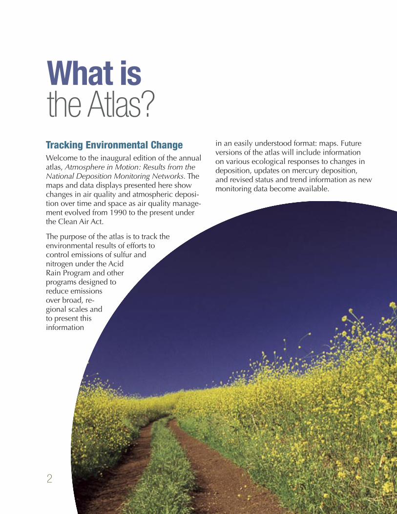
Tracking Environmental ChangeWelcome to the inaugural edition of the annual atlas, Atmosphere in Motion: Results from the National Deposition Monitoring Networks. The maps and data displays presented here show changes in air quality and atmospheric deposi-tion over time and space as air quality manage-ment evolved from 1990 to the present under the Clean Air Act.

The purpose of the atlas is to track the environmental results of efforts to control emissions of sulfur and nitrogen under the Acid Rain Program and other programs designed to reduce emissions over broad, re-gional scales and to present this information

in an easily understood format: maps. Future versions of the atlas will include information on various ecological responses to changes in deposition, updates on mercury deposition, and revised status and trend information as new monitoring data become available.

What isthe Atlas?

2

3

The Importance of Long-term MonitoringNational, long-term environmental monitoring networks are important tools for understanding how changes in emissions affect environmental quality over time and space. These networks are integral components of the “chain of account-

ability” used to characterize the relationships between emission sources and environ-

mental effects. Originally devel-oped for understanding acidi-

fication in the Northeast, the networks have since

expanded to provide invaluable infor-

mation relevant to a variety

of environ-mental

effects—

such as eutrophication, nitrogen saturation, ozone bio-injuries, and mercury contamina-tion—over a range of scales. The networks offer more than two decades of data based on con-sistent, standard field and lab procedures and quality-assured practices.

Since changes in the atmosphere can hap-pen very slowly, and trends are often obscured by the wide variability of measurements and regional climate, many years of continuous and consistent data are necessary to discern trends. Long-term monitoring networks are thus especially important for characterizing deposi-tion levels and identifying relationships among emissions, atmospheric loadings, and effects on human health and ecosystems. The Clean Air Status and Trends Network (CASTNET) and the National Atmospheric Deposition Program/Na-tional Trends Network (NADP/NTN) are two routine, long-term networks that EPA and its partners use to track geographic patterns and temporal trends in regional air quality and at-mospheric deposition in response to changes in emissions of sulfur dioxide (SO2) and nitrogen oxides (NOX). These networks provide a vital performance measure that is useful in assess-ing and reporting the effectiveness of current regulatory programs to improve air quality and reduce atmospheric inputs to ecosystems. They also provide the data needed to inform develop-ment of new policy initiatives.

4

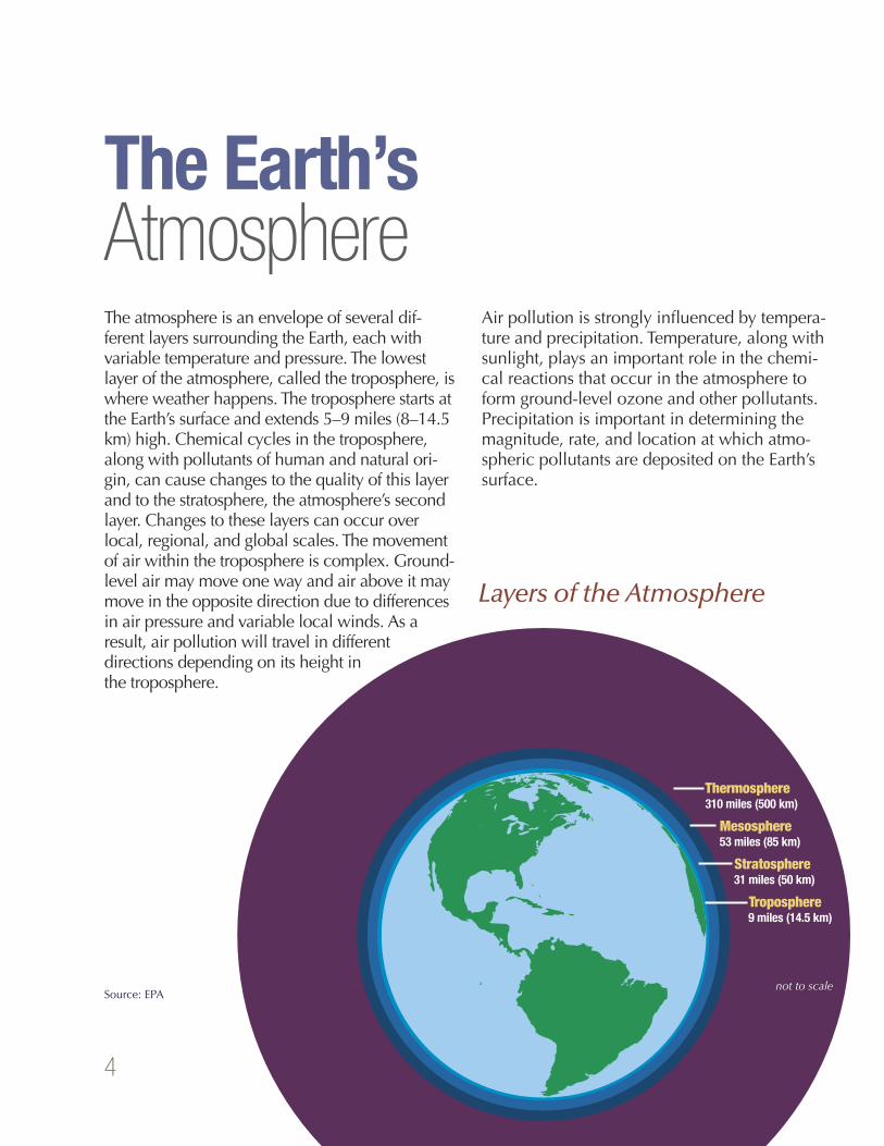
The atmosphere is an envelope of several dif-ferent layers surrounding the Earth, each with variable temperature and pressure. The lowest layer of the atmosphere, called the troposphere, is where weather happens. The troposphere starts at the Earth’s surface and extends 5–9 miles (8–14.5 km) high. Chemical cycles in the troposphere, along with pollutants of human and natural ori-gin, can cause changes to the quality of this layer and to the stratosphere, the atmosphere’s second layer. Changes to these layers can occur over local, regional, and global scales. The movement of air within the troposphere is complex. Ground-level air may move one way and air above it may move in the opposite direction due to differences in air pressure and variable local winds. As a result, air pollution will travel in different directions depending on its height in the troposphere.

Air pollution is strongly influenced by tempera-ture and precipitation. Temperature, along with sunlight, plays an important role in the chemi-cal reactions that occur in the atmosphere to form ground-level ozone and other pollutants. Precipitation is important in determining the magnitude, rate, and location at which atmo-spheric pollutants are deposited on the Earth’s surface.

The Earth’sAtmosphere

Layers of the Atmosphere

not to scaleSource: EPA

5

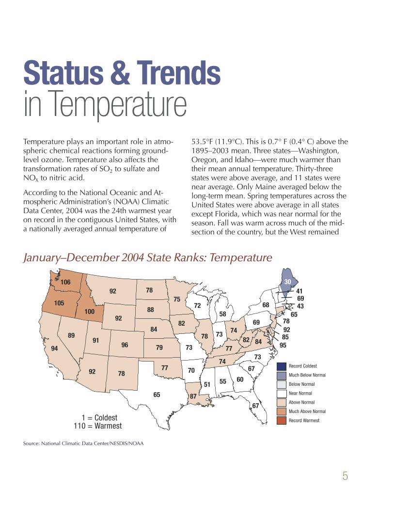
Temperature plays an important role in atmo-spheric chemical reactions forming ground-level ozone. Temperature also affects the transformation rates of SO2 to sulfate and NOX to nitric acid.

According to the National Oceanic and At-mospheric Administration’s (NOAA) Climatic Data Center, 2004 was the 24th warmest year on record in the contiguous United States, with a nationally averaged annual temperature of

53.5°F (11.9°C). This is 0.7° F (0.4° C) above the 1895–2003 mean. Three states—Washington, Oregon, and Idaho—were much warmer than their mean annual temperature. Thirty-three states were above average, and 11 states were near average. Only Maine averaged below the long-term mean. Spring temperatures across the United States were above average in all states except Florida, which was near normal for the season. Fall was warm across much of the mid-section of the country, but the West remained

January–December 2004 State Ranks: Temperature

Status & Trendsin Temperature

Source: National Climatic Data Center/NESDIS/NOAA

6

near average. Winter began relatively warm for states from the Upper Midwest to the East Coast.

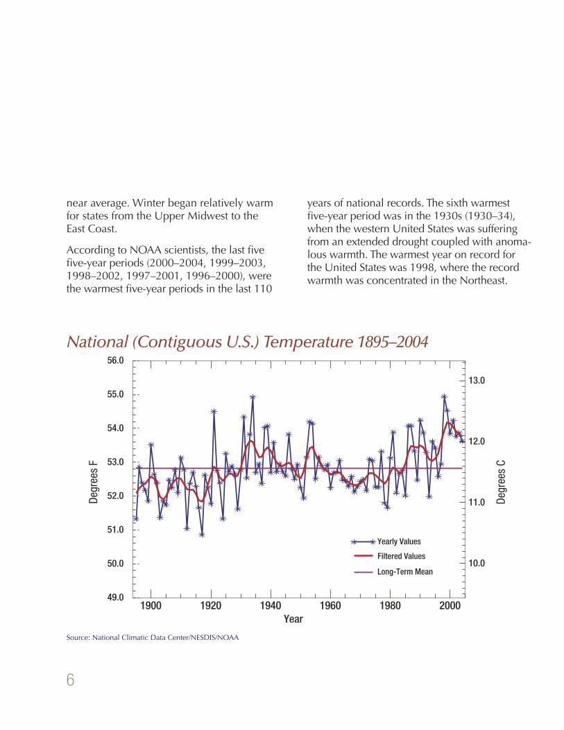
According to NOAA scientists, the last five five-year periods (2000–2004, 1999–2003, 1998–2002, 1997–2001, 1996–2000), were the warmest five-year periods in the last 110

years of national records. The sixth warmest five-year period was in the 1930s (1930–34), when the western United States was suffering from an extended drought coupled with anoma-lous warmth. The warmest year on record for the United States was 1998, where the record warmth was concentrated in the Northeast.

National (Contiguous U.S.) Temperature 1895–2004

Source: National Climatic Data Center/NESDIS/NOAA

7

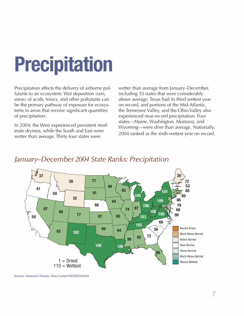
PrecipitationPrecipitation affects the delivery of airborne pol-lutants to an ecosystem. Wet deposition (rain, snow) of acids, toxics, and other pollutants can be the primary pathway of exposure for ecosys-tems in areas that receive significant quantities of precipitation.

In 2004, the West experienced persistent mod-erate dryness, while the South and East were wetter than average. Thirty-four states were

wetter than average from January–December, including 10 states that were considerably above average. Texas had its third wettest year on record, and portions of the Mid-Atlantic, the Tennessee Valley, and the Ohio Valley also experienced near-record precipitation. Four states—Maine, Washington, Montana, and Wyoming—were drier than average. Nationally, 2004 ranked as the sixth-wettest year on record.

���� ��

�� ��

��

��

��

��

��

�� ��

��

�� ���

���

��

��

�����

��

��

��

��

����

��

��

���

���

��

��

���

��

��

�����

��

��

���

���

��

��

���

��

���

��

��

���������������������������

�������������

�����������������

������������

�����������

������������

�����������������

��������������

January–December 2004 State Ranks: Precipitation

Source: National Climatic Data Center/NESDIS/NOAA

8

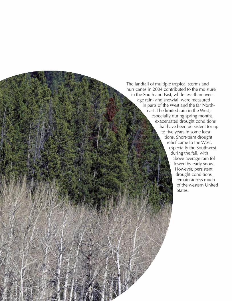
The landfall of multiple tropical storms and hurricanes in 2004 contributed to the moisture

in the South and East, while less-than-aver-age rain- and snowfall were measured

in parts of the West and the far North-east. The limited rain in the West,

especially during spring months, exacerbated drought conditions

that have been persistent for up to five years in some loca-

tions. Short-term drought relief came to the West, especially the Southwest during the fall, with above-average rain fol-lowed by early snow. However, persistent drought conditions remain across much of the western United States.

9

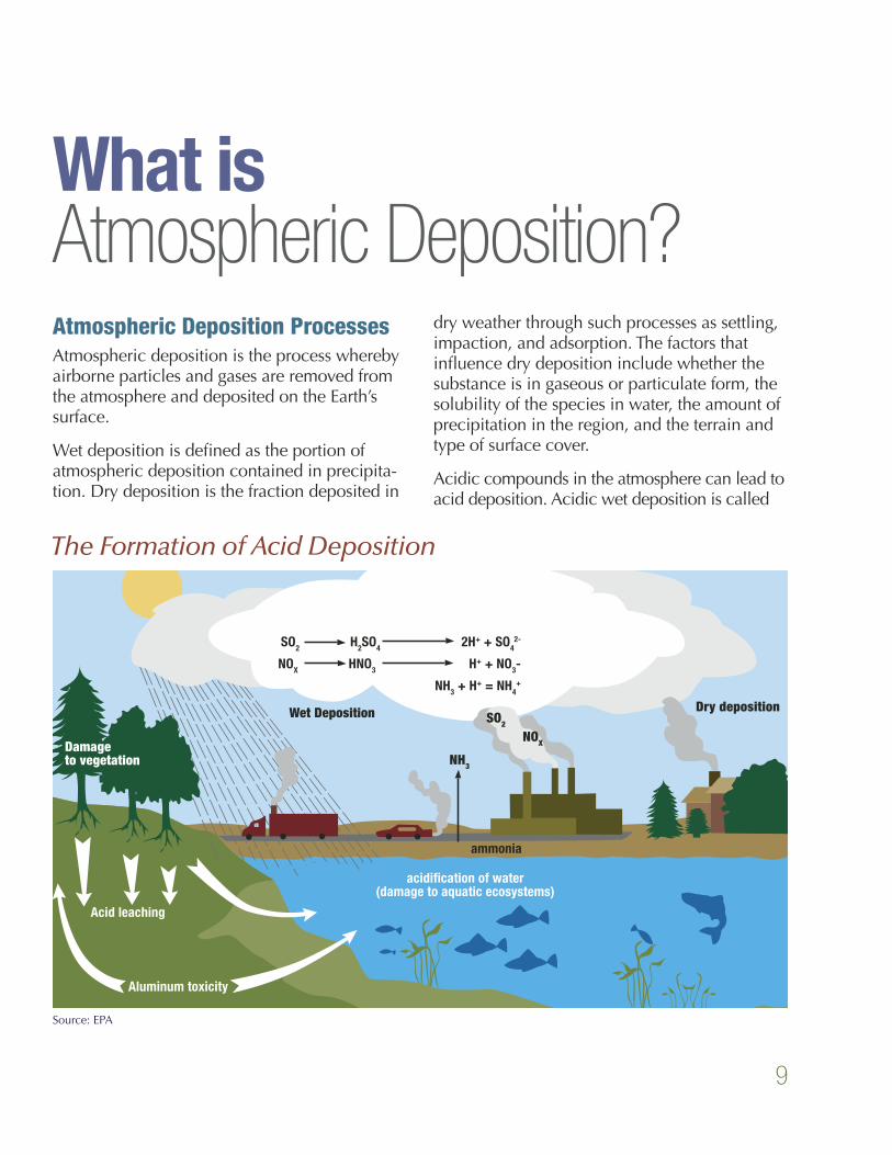
What isAtmospheric Deposition?Atmospheric Deposition ProcessesAtmospheric deposition is the process whereby airborne particles and gases are removed from the atmosphere and deposited on the Earth’s surface.

Wet deposition is defined as the portion of atmospheric deposition contained in precipita-tion. Dry deposition is the fraction deposited in

dry weather through such processes as settling, impaction, and adsorption. The factors that influence dry deposition include whether the substance is in gaseous or particulate form, the solubility of the species in water, the amount of precipitation in the region, and the terrain and type of surface cover.

Acidic compounds in the atmosphere can lead to acid deposition. Acidic wet deposition is called

The Formation of Acid Deposition

Source: EPA

10

acid precipitation or, more commonly, acid rain. Acidity in precipitation is measured by collect-ing samples of rain and measuring its pH, which is lower when acidic compounds are present. “Clean” or unpolluted rain has a slightly acidic pH of 5.6, because carbon dioxide and water in the air react together to form carbonic acid, a weak acid. Throughout much of the eastern United States, pH in rain is less than 4.5.

Acid deposition occurs when SO2, NOX, and ammonia (NH3) in the atmosphere react to form sulfuric acid (H2SO4), nitric acid (HNO3), and ammonium (NH4). These pollutants originate from natural sources (such as forest fires and volcanoes) as well as anthropogenic ones (such as the burning of fossil fuels in power plants and motor vehicles, and agricultural practices).

They are transported from the atmosphere and deposited to the Earth’s surface in particles, gases, rain, snow, clouds, and fog. Once these compounds enter an ecosystem, they can

acidify soil and surface waters, leading to a cascade of adverse ecological ef-

fects. Low pH in lakes and streams harms fish and other aquatic

organisms, alters forest soils, degrades the growing con-

ditions for some tree spe-cies, and affects other

vegetation.

11

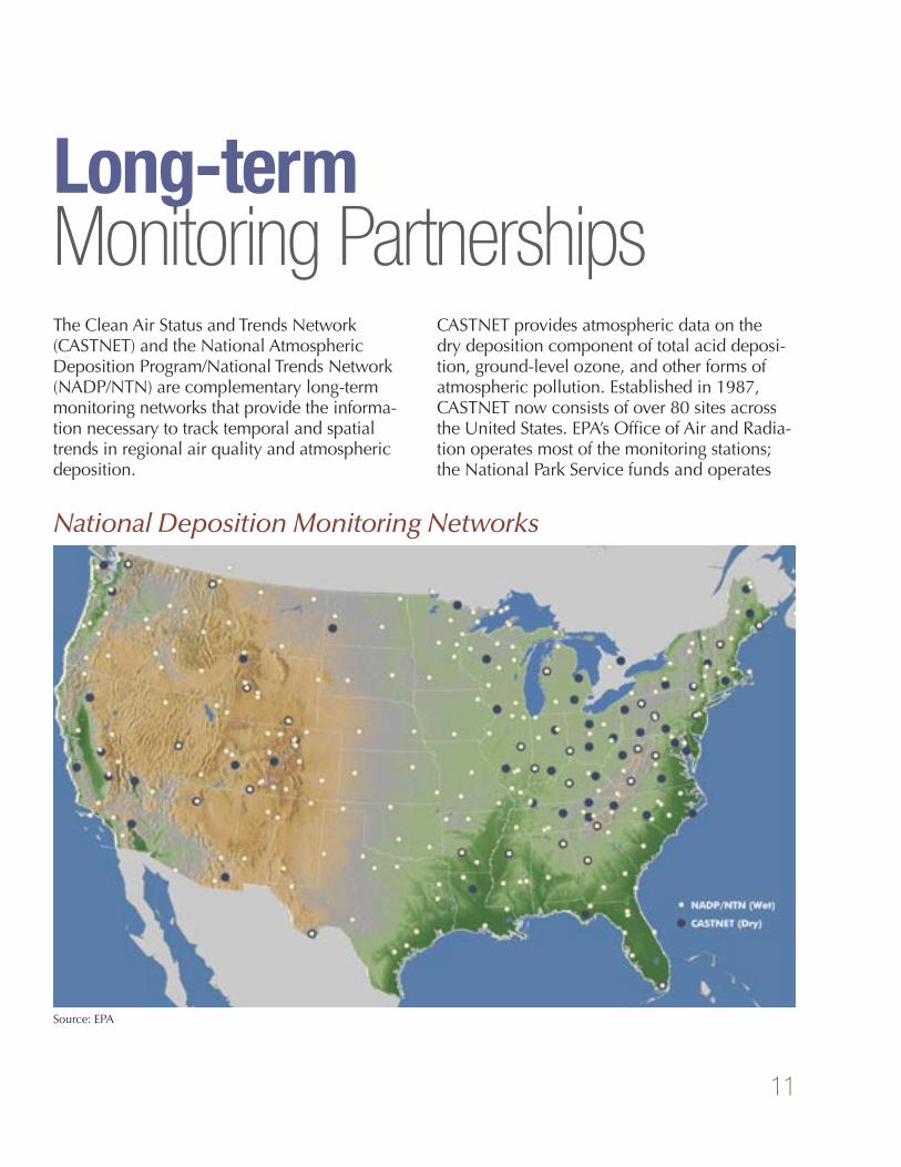
Long-termMonitoring PartnershipsThe Clean Air Status and Trends Network (CASTNET) and the National Atmospheric Deposition Program/National Trends Network (NADP/NTN) are complementary long-term monitoring networks that provide the informa-tion necessary to track temporal and spatial trends in regional air quality and atmospheric deposition.

CASTNET provides atmospheric data on the dry deposition component of total acid deposi-tion, ground-level ozone, and other forms of atmospheric pollution. Established in 1987, CASTNET now consists of over 80 sites across the United States. EPA’s Office of Air and Radia-tion operates most of the monitoring stations; the National Park Service funds and operates

National Deposition Monitoring Networks

Source: EPA

12

approximately 30 stations in cooperation with EPA. Many CASTNET sites are approaching a continuous 20-year data record, reflecting EPA’s commitment to long-term environmen-tal monitoring.

NADP/NTN is a nationwide, long-term net-work monitoring the chemistry of precipita-tion. The network is a cooperative effort in-volving many groups, including the State Agricultural Experiment Stations, U.S. Geologi-cal Survey, U.S. Department of Agriculture, EPA, NPS, NOAA, and other governmental and private entities. The NADP/NTN has grown from 22 stations at the end of 1978 to more than 250 sites spanning the continental United States, Alaska, Puerto Rico, and the Virgin Islands.

The monitoring sites of both CASTNET and NADP/NTN are located to represent ma-jor physiographic, agricultural, aquatic, and forested areas within each cooperating state, region, or ecoregion.

Wherever possible, monitoring sites are co-located with other monitoring and research programs to optimize existing monitoring resources and help scientists

capture a wider variety of data from a given location. They also are located using criteria to minimize impacts from local emission sources, typically in areas where urban influences are minimal. In effect, these networks provide regionally representative data. Each network offers a rigorous quality assurance program, including consistent, standardized and trans-parent field and lab procedures that as-sure the comparability of data across network sites.

13

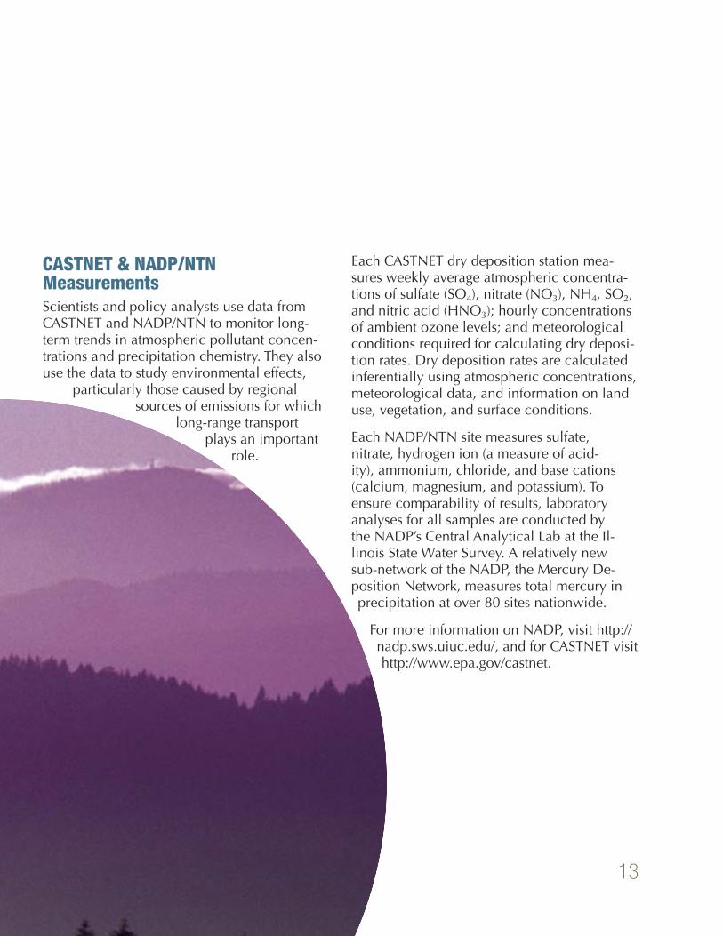
CASTNET & NADP/NTN MeasurementsScientists and policy analysts use data from CASTNET and NADP/NTN to monitor long-term trends in atmospheric pollutant concen-trations and precipitation chemistry. They also use the data to study environmental effects,

particularly those caused by regional sources of emissions for which

long-range transport plays an important

role.

Each CASTNET dry deposition station mea-sures weekly average atmospheric concentra-tions of sulfate (SO4), nitrate (NO3), NH4, SO2, and nitric acid (HNO3); hourly concentrations of ambient ozone levels; and meteorological conditions required for calculating dry deposi-tion rates. Dry deposition rates are calculated inferentially using atmospheric concentrations, meteorological data, and information on land use, vegetation, and surface conditions.

Each NADP/NTN site measures sulfate, nitrate, hydrogen ion (a measure of acid-ity), ammonium, chloride, and base cations (calcium, magnesium, and potassium). To ensure comparability of results, laboratory analyses for all samples are conducted by the NADP’s Central Analytical Lab at the Il-linois State Water Survey. A relatively new sub-network of the NADP, the Mercury De-position Network, measures total mercury in precipitation at over 80 sites nationwide.

For more information on NADP, visit http://nadp.sws.uiuc.edu/, and for CASTNET visit http://www.epa.gov/castnet.

14

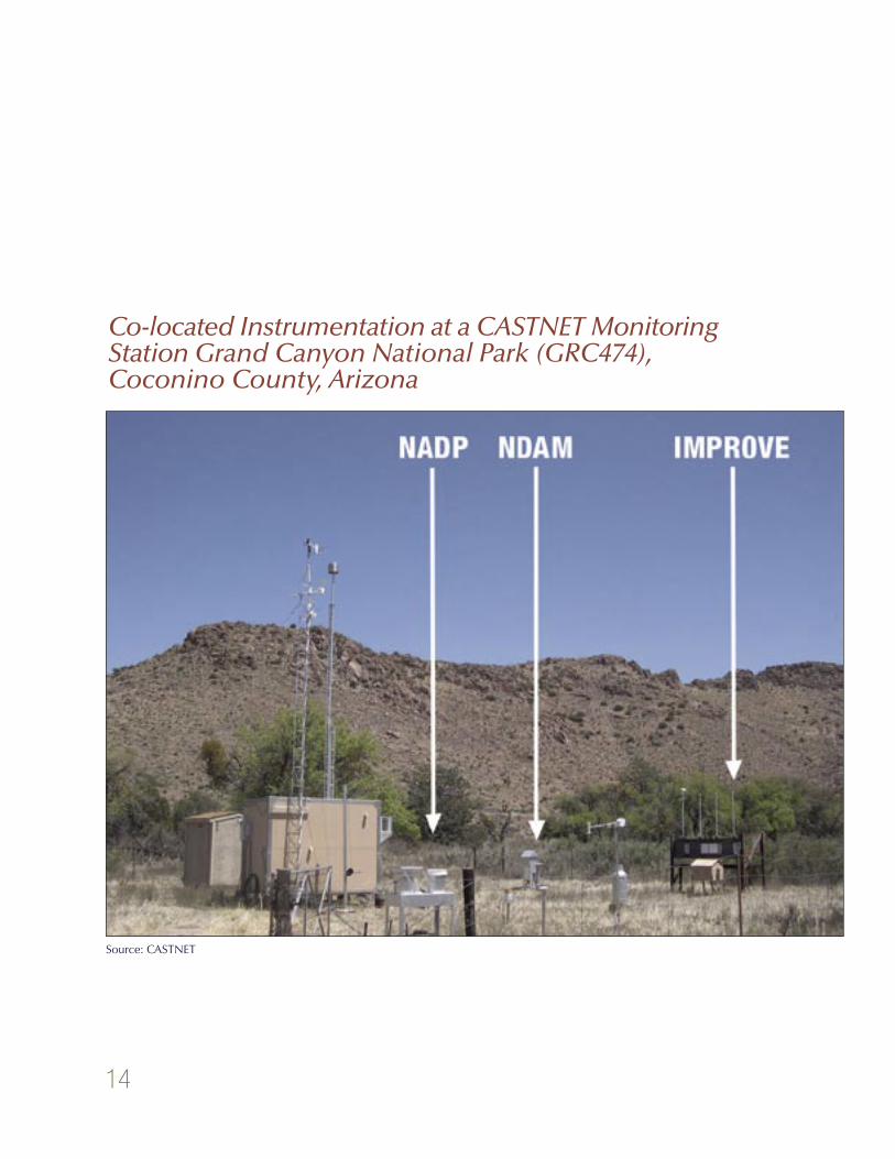
Co-located Instrumentation at a CASTNET Monitoring Station Grand Canyon National Park (GRC474), Coconino County, Arizona

Source: CASTNET

15

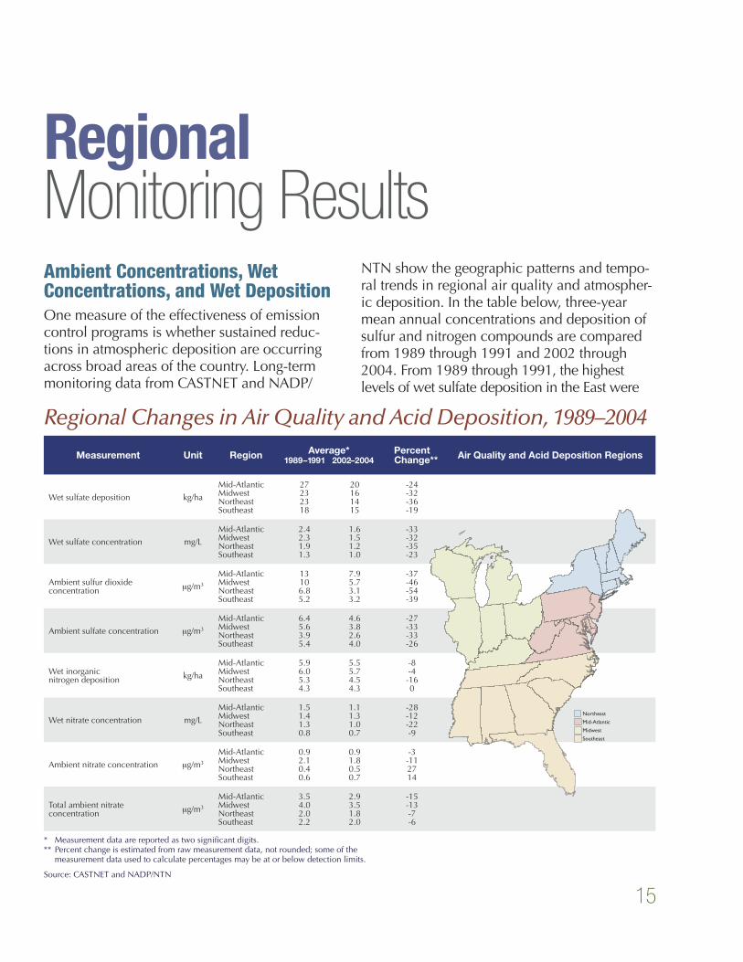
RegionalMonitoring ResultsAmbient Concentrations, Wet Concentrations, and Wet DepositionOne measure of the effectiveness of emission control programs is whether sustained reduc-tions in atmospheric deposition are occurring across broad areas of the country. Long-term monitoring data from CASTNET and NADP/

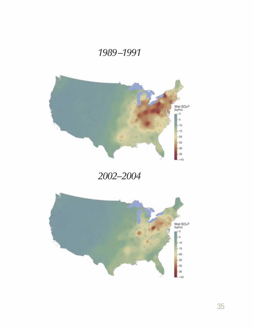
NTN show the geographic patterns and tempo-ral trends in regional air quality and atmospher-ic deposition. In the table below, three-year mean annual concentrations and deposition of sulfur and nitrogen compounds are compared from 1989 through 1991 and 2002 through 2004. From 1989 through 1991, the highest levels of wet sulfate deposition in the East were

Regional Changes in Air Quality and Acid Deposition, 1989–2004

Measurement Unit Region Average*1989–1991 2002–2004

Percent Change** Air Quality and Acid Deposition Regions

Wet sulfate deposition kg/ha

Mid-AtlanticMidwestNortheastSoutheast

27232318

20161415

-24-32-36-19

Wet sulfate concentration mg/L

Mid-AtlanticMidwestNortheastSoutheast

2.42.31.91.3

1.61.51.21.0

-33-32-35-23

Ambient sulfur dioxide concentration μg/m3

Mid-AtlanticMidwestNortheastSoutheast

13106.85.2

7.95.73.13.2

-37-46-54-39

Ambient sulfate concentration μg/m3

Mid-AtlanticMidwestNortheastSoutheast

6.45.63.95.4

4.63.82.64.0

-27-33-33-26

Wet inorganic nitrogen deposition kg/ha

Mid-AtlanticMidwestNortheastSoutheast

5.96.05.34.3

5.55.74.54.3

-8-4-160

Wet nitrate concentration mg/L

Mid-AtlanticMidwestNortheastSoutheast

1.51.41.30.8

1.11.31.00.7

-28-12-22-9

Ambient nitrate concentration μg/m3

Mid-AtlanticMidwestNortheastSoutheast

0.92.10.40.6

0.91.80.50.7

-3-112714

Total ambient nitrate concentration μg/m3

Mid-AtlanticMidwestNortheastSoutheast

3.54.02.02.2

2.93.51.82.0

-15-13-7-6

* Measurement data are reported as two significant digits.** Percent change is estimated from raw measurement data, not rounded; some of the

measurement data used to calculate percentages may be at or below detection limits.

Source: CASTNET and NADP/NTN

16

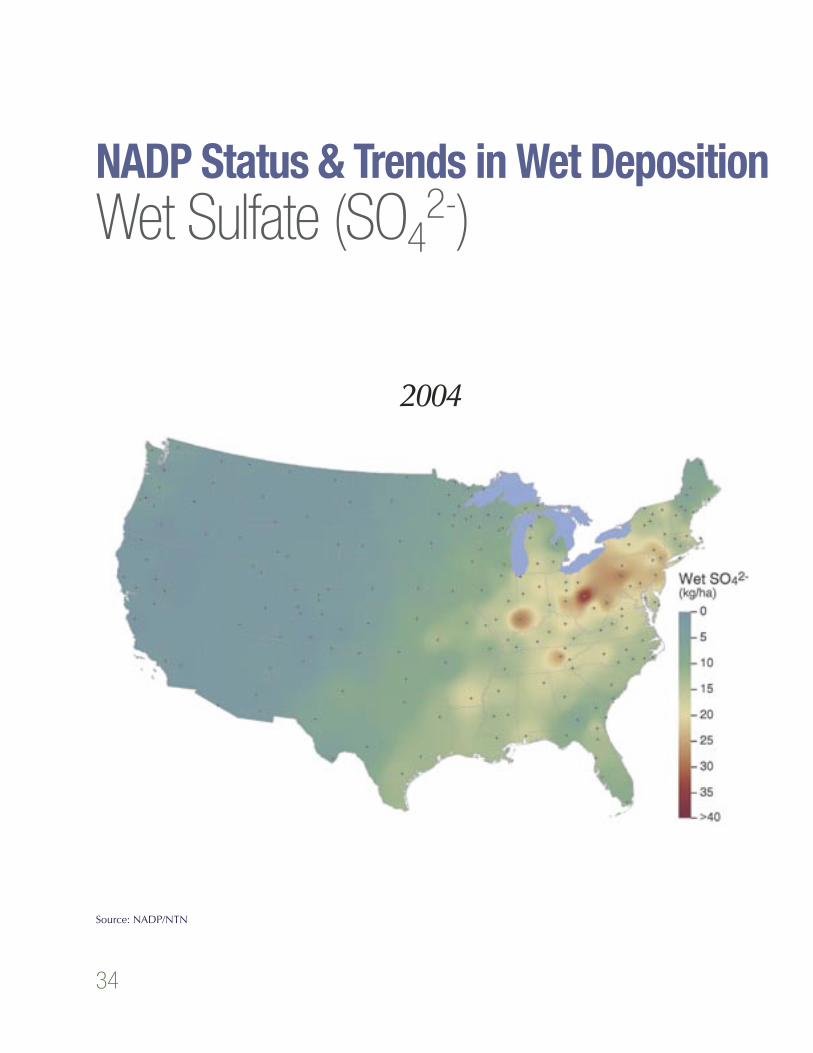
observed in parts of the Northeast, in the Mid-Atlantic near western Pennsylvania, and along the Ohio River Valley (see map on page 35). Since 1991, wet sulfate deposition has decreased significantly, with average levels in the eastern U.S. decreasing 36 percent in the Northeast, 24 percent in the Mid-Atlantic, and 32 percent in the Midwest. Like wet sulfate deposition, monitoring

data from CASTNET show that ambient sulfur dioxide and ambient sulfate concentrations

decreased throughout the eastern United States over the past decade, by an average of 30-40 percent. The more than 50 per-cent reduction in sulfur dioxide concen-trations in the Northeast is particularly noteworthy over this time period.

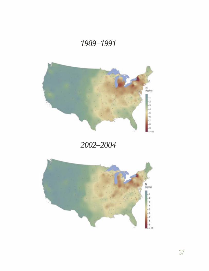
In contrast to the reduction of sulfur levels, reductions in the nitrogen deposition recorded since the early 1990’s have been less dramatic. Inorganic nitrogen deposition decreased modestly in the Mid-Atlantic and Northeast (averaging 8-16 percent), but remained virtu-ally unchanged in other regions. Total ambient nitrate concentrations (nitric acid + particulate nitrate), an indicator of NOx emissions changes,

also decreased modestly, particularly in the Mid-Atlantic (by an average of

15 percent), and in the Midwest (by an average of 13 percent). Other regions

have not shown much change.

17

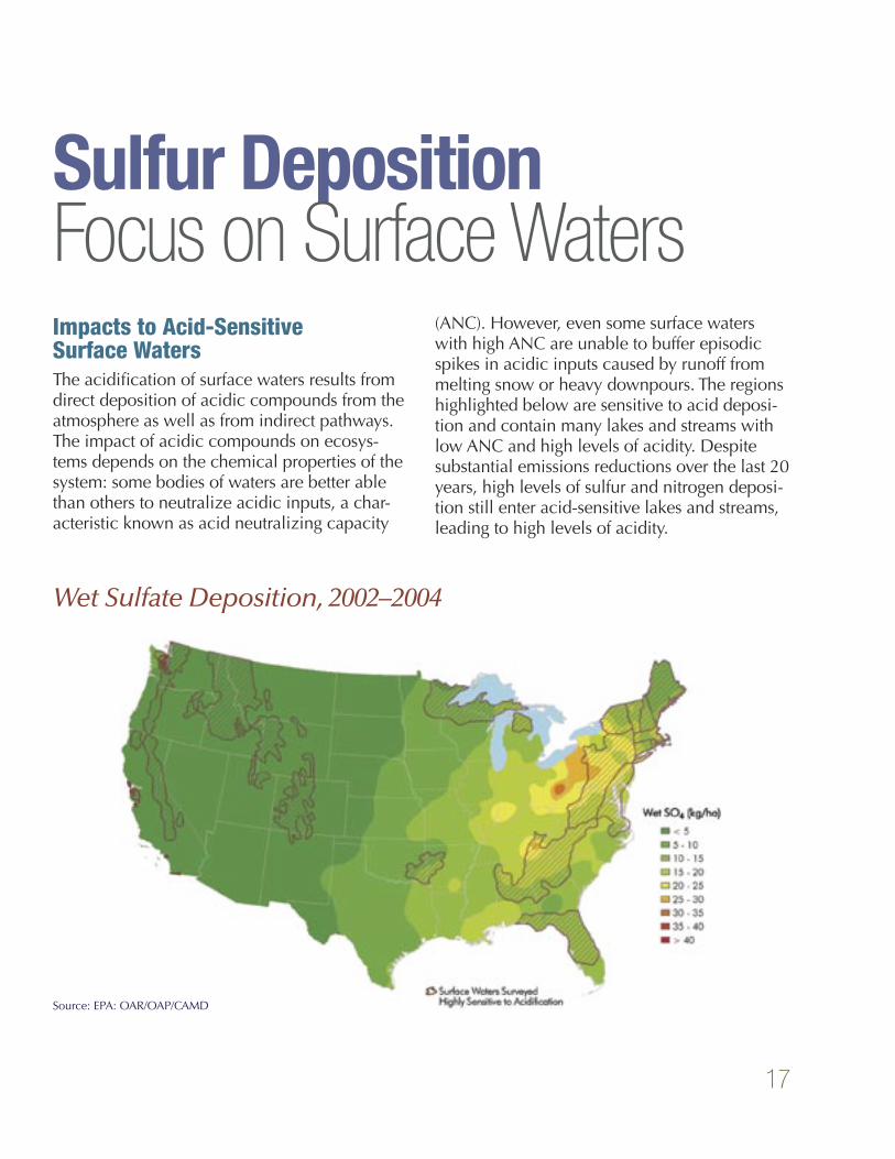
Impacts to Acid-Sensitive Surface WatersThe acidification of surface waters results from direct deposition of acidic compounds from the atmosphere as well as from indirect pathways. The impact of acidic compounds on ecosys-tems depends on the chemical properties of the system: some bodies of waters are better able than others to neutralize acidic inputs, a char-acteristic known as acid neutralizing capacity

(ANC). However, even some surface waters with high ANC are unable to buffer episodic spikes in acidic inputs caused by runoff from melting snow or heavy downpours. The regions highlighted below are sensitive to acid deposi-tion and contain many lakes and streams with low ANC and high levels of acidity. Despite substantial emissions reductions over the last 20 years, high levels of sulfur and nitrogen deposi-tion still enter acid-sensitive lakes and streams, leading to high levels of acidity.

Wet Sulfate Deposition, 2002–2004

Sulfur DepositionFocus on Surface Waters

Source: EPA: OAR/OAP/CAMD

18

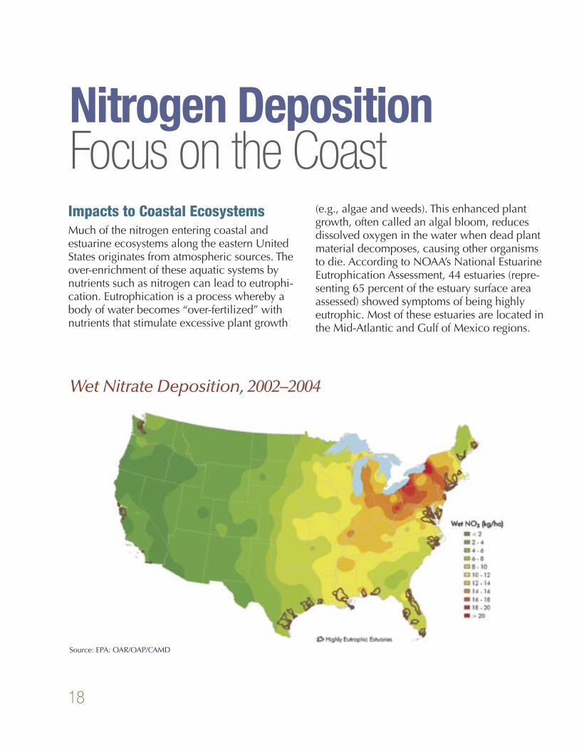
Impacts to Coastal EcosystemsMuch of the nitrogen entering coastal and estuarine ecosystems along the eastern United States originates from atmospheric sources. The over-enrichment of these aquatic systems by nutrients such as nitrogen can lead to eutrophi-cation. Eutrophication is a process whereby a body of water becomes “over-fertilized” with nutrients that stimulate excessive plant growth

(e.g., algae and weeds). This enhanced plant growth, often called an algal bloom, reduces dissolved oxygen in the water when dead plant material decomposes, causing other organisms to die. According to NOAA’s National Estuarine Eutrophication Assessment, 44 estuaries (repre-senting 65 percent of the estuary surface area assessed) showed symptoms of being highly eutrophic. Most of these estuaries are located in the Mid-Atlantic and Gulf of Mexico regions.

Wet Nitrate Deposition, 2002–2004

Nitrogen DepositionFocus on the Coast

Source: EPA: OAR/OAP/CAMD

19

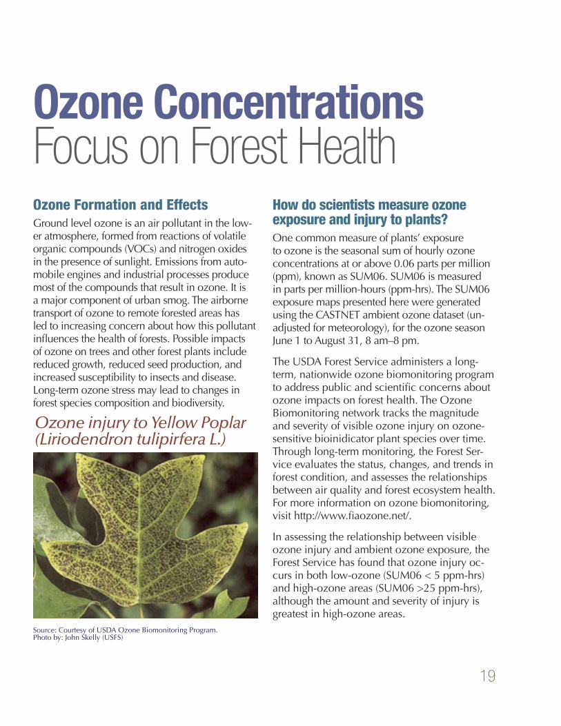
Ozone Formation and EffectsGround level ozone is an air pollutant in the low-er atmosphere, formed from reactions of volatile organic compounds (VOCs) and nitrogen oxides in the presence of sunlight. Emissions from auto-mobile engines and industrial processes produce most of the compounds that result in ozone. It is a major component of urban smog. The airborne transport of ozone to remote forested areas has led to increasing concern about how this pollutant influences the health of forests. Possible impacts of ozone on trees and other forest plants include reduced growth, reduced seed production, and increased susceptibility to insects and disease. Long-term ozone stress may lead to changes in forest species composition and biodiversity.

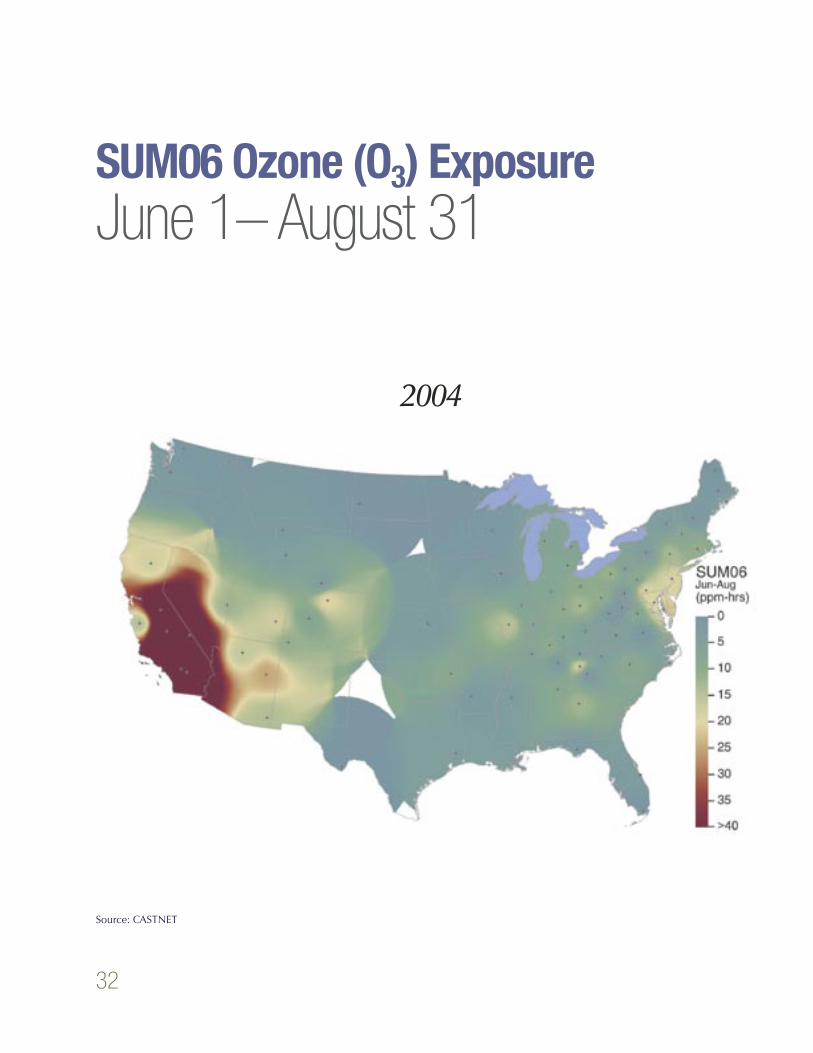
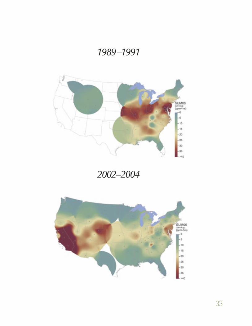
How do scientists measure ozone exposure and injury to plants?One common measure of plants’ exposure to ozone is the seasonal sum of hourly ozone concentrations at or above 0.06 parts per million (ppm), known as SUM06. SUM06 is measured in parts per million-hours (ppm-hrs). The SUM06 exposure maps presented here were generated using the CASTNET ambient ozone dataset (un-adjusted for meteorology), for the ozone season June 1 to August 31, 8 am–8 pm.

The USDA Forest Service administers a long-term, nationwide ozone biomonitoring program to address public and scientific concerns about ozone impacts on forest health. The Ozone Biomonitoring network tracks the magnitude and severity of visible ozone injury on ozone-sensitive bioinidicator plant species over time. Through long-term monitoring, the Forest Ser-vice evaluates the status, changes, and trends in forest condition, and assesses the relationships between air quality and forest ecosystem health. For more information on ozone biomonitoring, visit http://www.fiaozone.net/.

In assessing the relationship between visible ozone injury and ambient ozone exposure, the Forest Service has found that ozone injury oc-curs in both low-ozone (SUM06 < 5 ppm-hrs) and high-ozone areas (SUM06 >25 ppm-hrs), although the amount and severity of injury is greatest in high-ozone areas.

Ozone ConcentrationsFocus on Forest Health

Ozone injury to Yellow Poplar (Liriodendron tulipirfera L.)

Source: Courtesy of USDA Ozone Biomonitoring Program. Photo by: John Skelly (USFS)

20

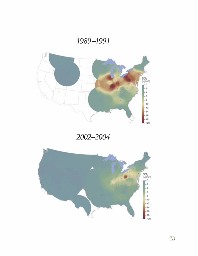
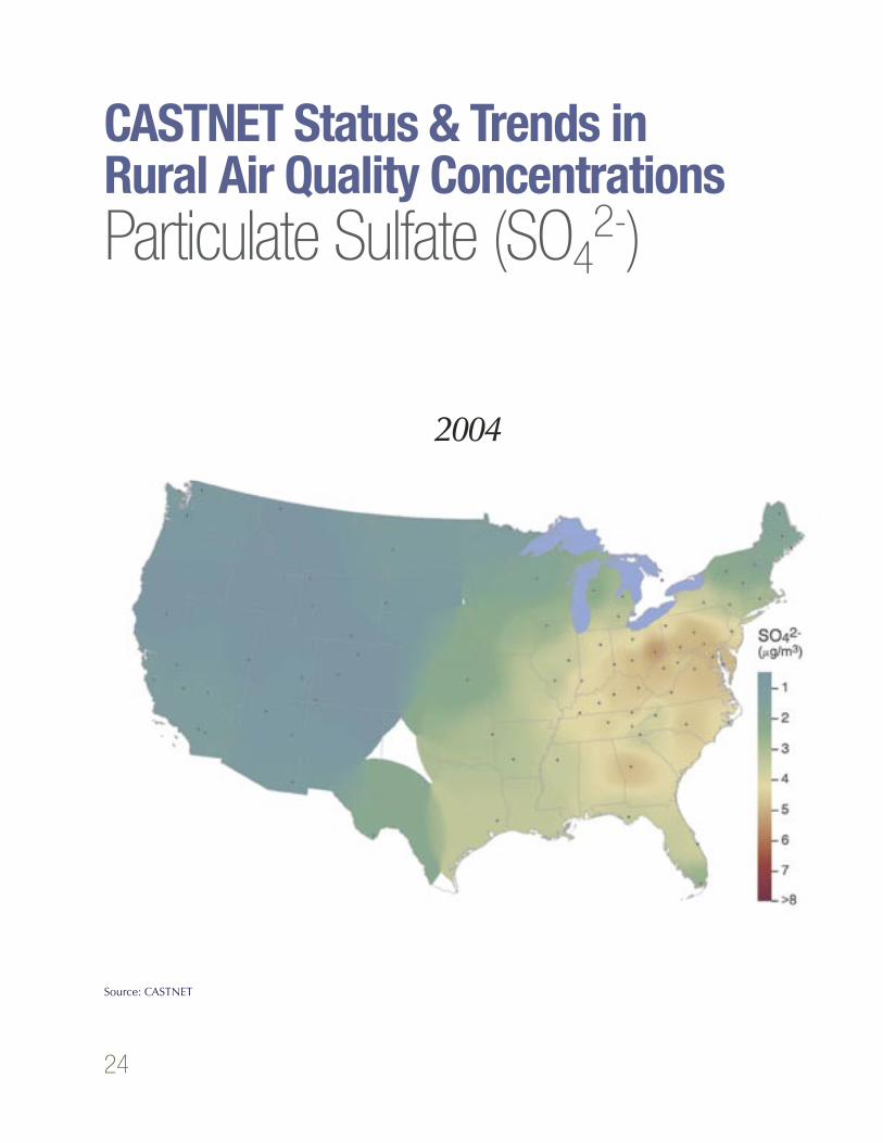
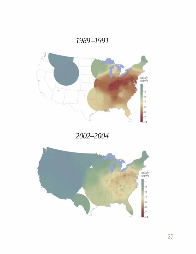
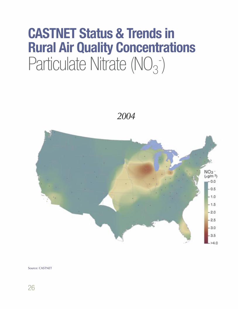
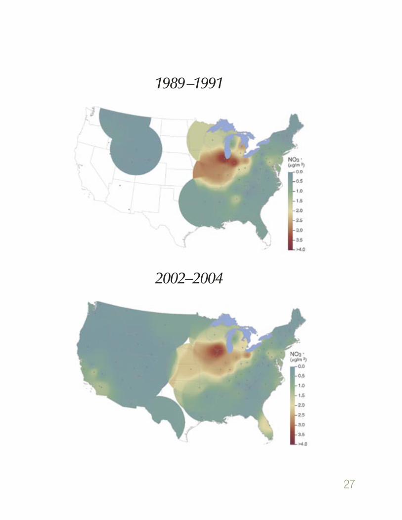
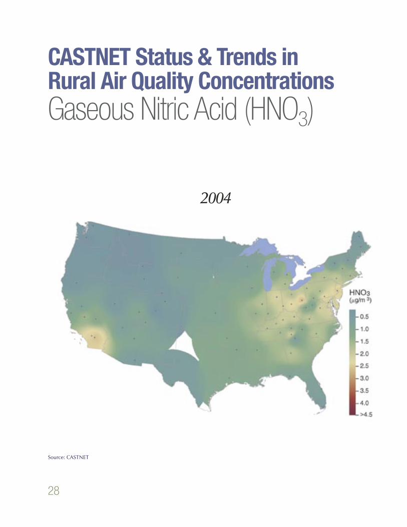
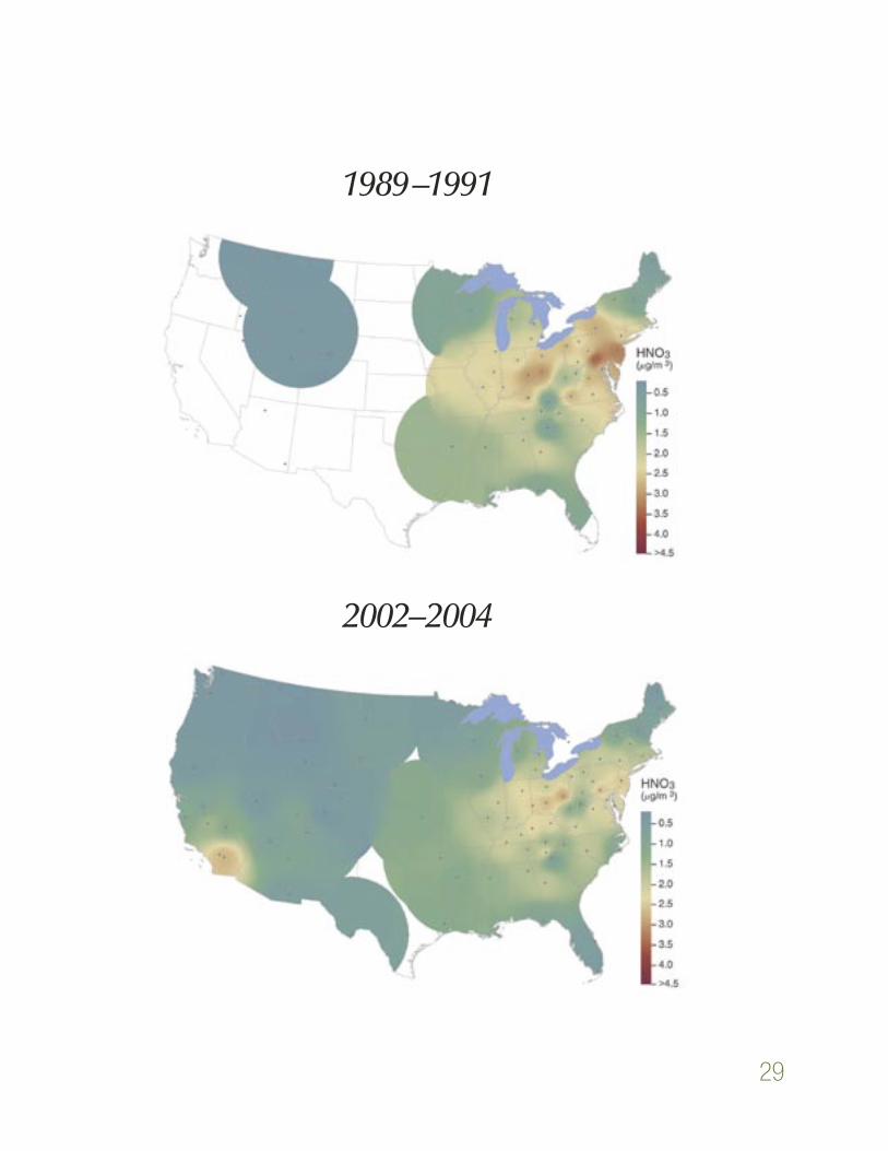
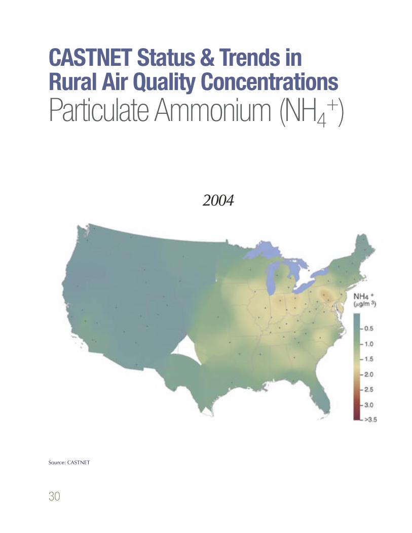
Regional Air Quality and Total Atmospheric DepositionThe status and trend maps on the follow-ing pages show the geographic variability in ambient air concentrations of SO2, SO4, NO3, HNO3, NH4, and ozone from CASTNET mea-surements; wet nitrogen and sulfate deposition from NADP/NTN measurements; and total sul-fur and nitrogen deposition (wet and dry) from co-located CASTNET and NADP/NTN moni-toring stations. The status maps depict mea-surements for 2004. The trend maps cover two three-year averaging periods: 1989–1991 and 2002–2004. The measurement units are μg/m3 for ambient air concentrations and kg/ha for wet and total deposition (the amount of pollut-ant deposited over an area).

Ambient Air ConcentrationsThe CASTNET ambient concentration maps were generated in ArcInfo GIS software using an inverse distance weighting (IDW) interpolation technique. Using IDW, the surface is most influ-enced by the nearest point values and less so by more distant points. In developing the trend map surfaces, the point concentration values for each year in the three-year period were gridded to a 10 km2 surface. CASTNET sites within 400 km of each grid point were used in the computation. The three annual grids from the three-year period were averaged to derive the mean concentration of the three-year period. Only sites meeting com-pleteness criteria for at least two of the three years of the averaging period were included. See the CASTNET website for information on com-pleteness crite-ria. Color

Methods of MappingStatus & Trends

Ambient air concentration is the principal measure of air quality. It is the monitored amount of pollutant in the air reported in micrograms per cubic meter (μg/m3) or parts per million (ppm).

Atmospheric deposition is the amount of air pollution hitting the Earth’s surface reported in kilograms per hectare (kg/ha). Wet concentration, presented in milligrams per liter (mg/L), is the amount of pollutant in a standard volume.

21

contours represent the classes of concentration values indicated in the legend. The color is ramped from green to red, representing the range of concentration values from low to high.

Only grid points within 400 km for all three years were included in the averages; grid points for which no estimate is made are represented by white. These are areas for which no data exist due to gaps in CASTNET monitoring coverage (i.e., low site density, particularly in early years as the network was growing).

Wet DepositionSimilar to CASTNET concentration maps, the

NADP/NTN wet deposition maps were gener-ated in ArcInfo using an IDW

interpolation technique. In developing the

trend map

surfaces, the point deposition values for each year in the three-year period were gridded to a 10 km2 surface. NADP/NTN sites within 400 km of each grid point were used in the computation. The three annual grids from the three-year period were averaged to derive the mean concentration of the three-year period. See the NADP website for information about NTN completeness criteria.

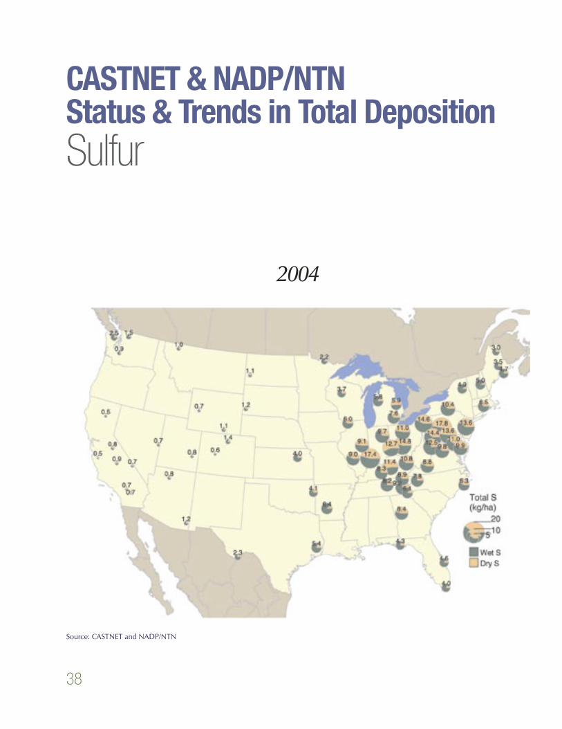
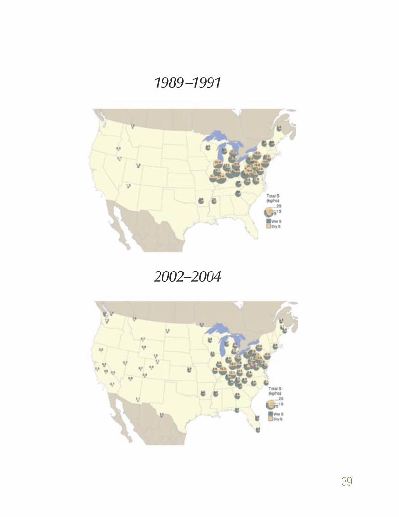
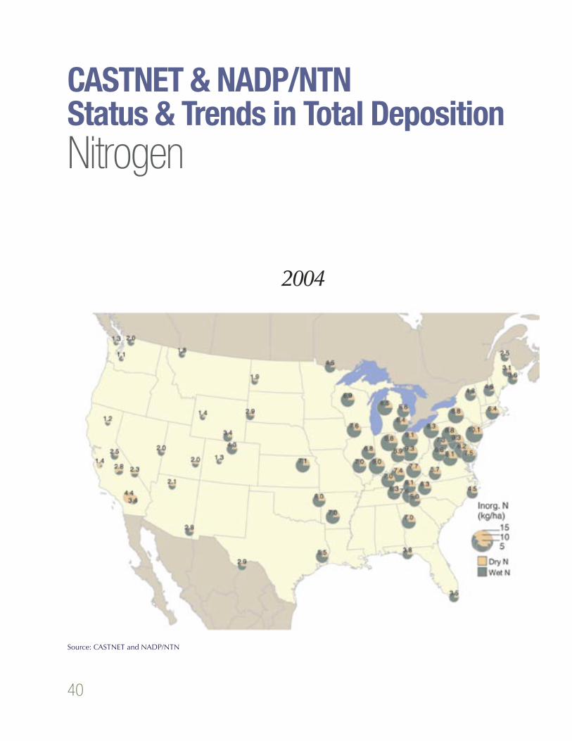
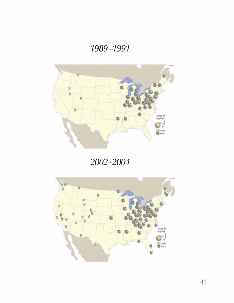
Total Deposition (Wet and Dry Sulfur and Nitrogen)The total deposition maps created in ArcInfo show scaled pie charts of sulfur (S) and nitro-gen (N) deposition at co-located CASTNET and NADP/NTN monitoring stations. Each pie chart consists of total S or N deposition at a single point location. The wet deposition component is derived from a wet concentration grid us-ing the IDW technique mentioned above. The interpolated value on the wet concentration surface at a co-located CASTNET site is then multiplied by measured precipitation at that site. The dry deposition component is from CASTNET, derived from an inferential model.

Only sites meeting completeness criteria for at least two of the three years of the averaging

period were included. Note that total N deposition maps are labeled as “total”

although ammonia (NH3), a major component of total nitrogen, is not

measured by any networks. Meth-ods for routine measurement of

NH3 in a network mode are needed.

22

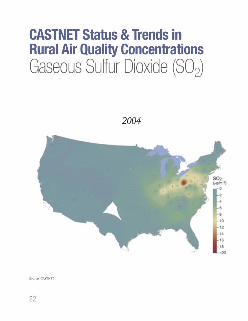
CASTNET Status & Trends in Rural Air Quality ConcentrationsGaseous Sulfur Dioxide (SO2)

2004

Source: CASTNET

23

1989–1991

2002–2004

24

CASTNET Status & Trends in Rural Air Quality ConcentrationsParticulate Sulfate (SO4

2-)

2004

Source: CASTNET

25

1989–1991

2002–2004

26

CASTNET Status & Trends in Rural Air Quality ConcentrationsParticulate Nitrate (NO3

-)

2004

Source: CASTNET

27

1989–1991

2002–2004

28

CASTNET Status & Trends in Rural Air Quality ConcentrationsGaseous Nitric Acid (HNO3)

2004

Source: CASTNET

29

1989–1991

2002–2004

30

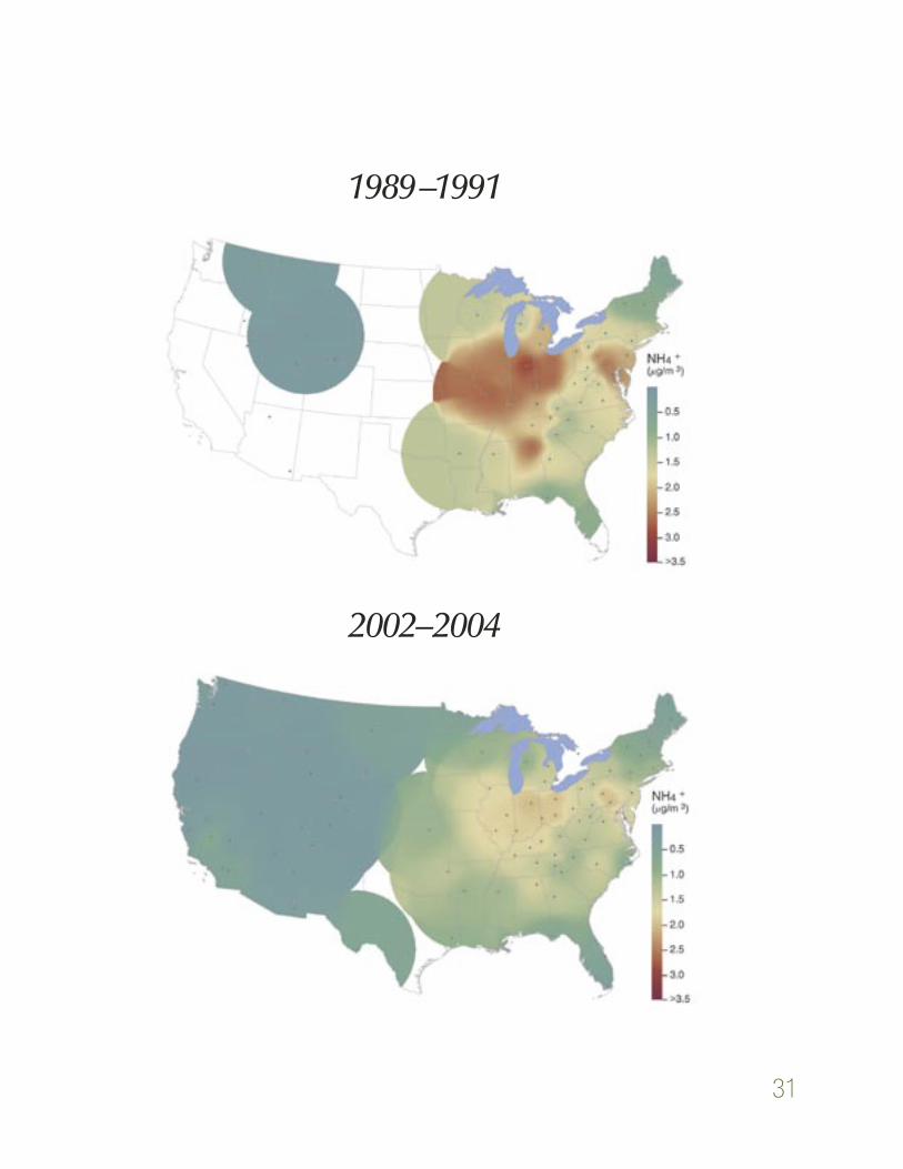
CASTNET Status & Trends in Rural Air Quality ConcentrationsParticulate Ammonium (NH4

+)

2004

Source: CASTNET

31

1989–1991

2002–2004

32

SUM06 Ozone (O3) ExposureJune 1– August 31

2004

Source: CASTNET

33

1989–1991

2002–2004

34

NADP Status & Trends in Wet DepositionWet Sulfate (SO4

2-)

2004

Source: NADP/NTN

35

1989–1991

2002–2004

36

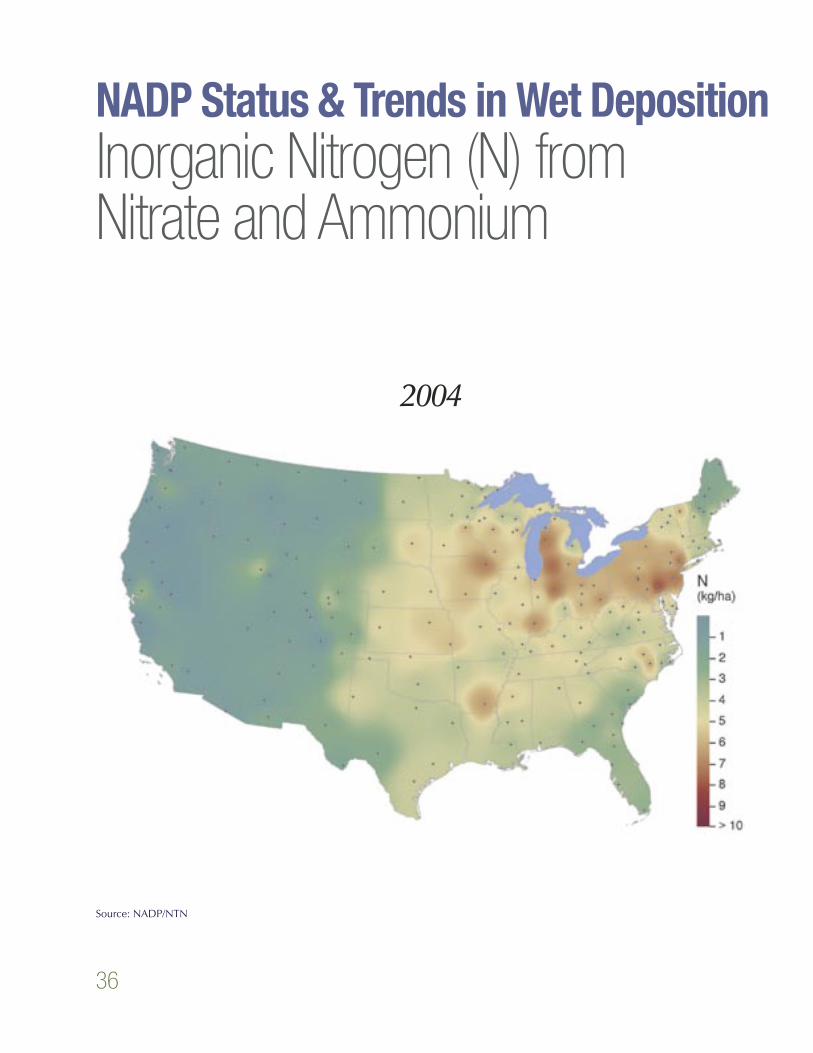
NADP Status & Trends in Wet DepositionInorganic Nitrogen (N) from Nitrate and Ammonium

2004

Source: NADP/NTN

37

1989–1991

2002–2004

38

CASTNET & NADP/NTN Status & Trends in Total DepositionSulfur

2004

Source: CASTNET and NADP/NTN

39

1989–1991

2002–2004

40

CASTNET & NADP/NTN Status & Trends in Total DepositionNitrogen

2004

Source: CASTNET and NADP/NTN

41

1989–1991

2002–2004

42

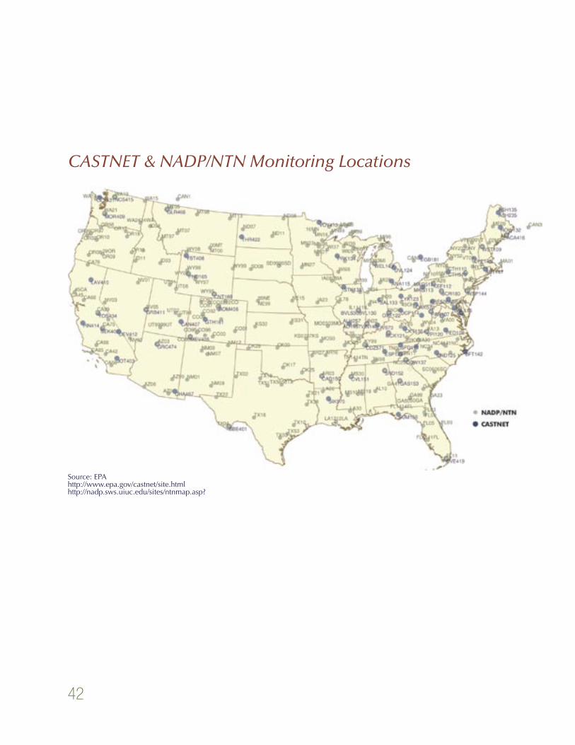
CASTNET & NADP/NTN Monitoring Locations

Source: EPAhttp://www.epa.gov/castnet/site.htmlhttp://nadp.sws.uiuc.edu/sites/ntnmap.asp?

43

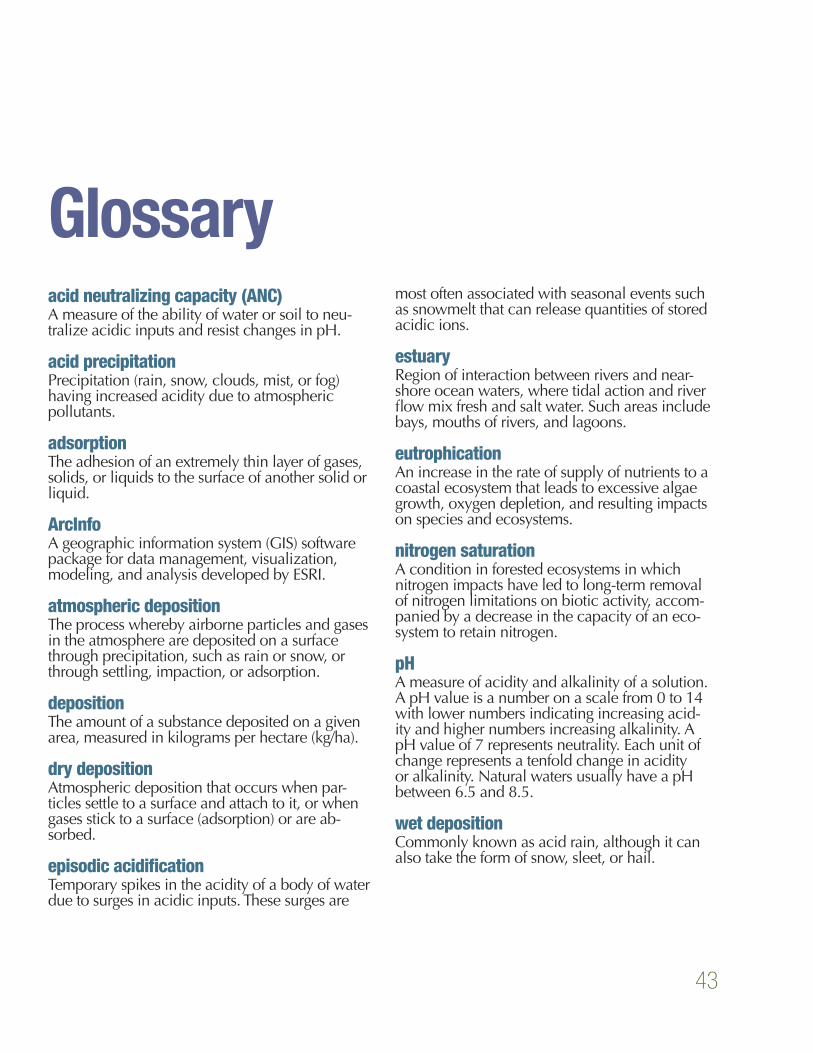
Glossaryacid neutralizing capacity (ANC) A measure of the ability of water or soil to neu-tralize acidic inputs and resist changes in pH.

acid precipitationPrecipitation (rain, snow, clouds, mist, or fog) having increased acidity due to atmospheric pollutants.

adsorptionThe adhesion of an extremely thin layer of gases, solids, or liquids to the surface of another solid or liquid.

ArcInfoA geographic information system (GIS) software package for data management, visualization, modeling, and analysis developed by ESRI.

atmospheric depositionThe process whereby airborne particles and gases in the atmosphere are deposited on a surface through precipitation, such as rain or snow, or through settling, impaction, or adsorption.

depositionThe amount of a substance deposited on a given area, measured in kilograms per hectare (kg/ha).

dry depositionAtmospheric deposition that occurs when par-ticles settle to a surface and attach to it, or when gases stick to a surface (adsorption) or are ab-sorbed.

episodic acidificationTemporary spikes in the acidity of a body of water due to surges in acidic inputs. These surges are

most often associated with seasonal events such as snowmelt that can release quantities of stored acidic ions.

estuaryRegion of interaction between rivers and near-shore ocean waters, where tidal action and river flow mix fresh and salt water. Such areas include bays, mouths of rivers, and lagoons.

eutrophication An increase in the rate of supply of nutrients to a coastal ecosystem that leads to excessive algae growth, oxygen depletion, and resulting impacts on species and ecosystems.

nitrogen saturationA condition in forested ecosystems in which nitrogen impacts have led to long-term removal of nitrogen limitations on biotic activity, accom-panied by a decrease in the capacity of an eco-system to retain nitrogen.

pHA measure of acidity and alkalinity of a solution. A pH value is a number on a scale from 0 to 14 with lower numbers indicating increasing acid-ity and higher numbers increasing alkalinity. A pH value of 7 represents neutrality. Each unit of change represents a tenfold change in acidity or alkalinity. Natural waters usually have a pH between 6.5 and 8.5.

wet depositionCommonly known as acid rain, although it can also take the form of snow, sleet, or hail.

44

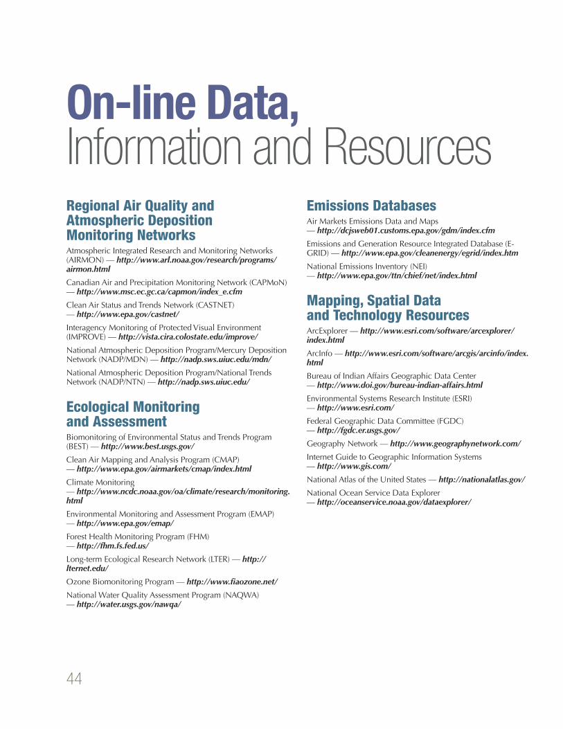
Regional Air Quality and Atmospheric Deposition Monitoring NetworksAtmospheric Integrated Research and Monitoring Networks (AIRMON) — http://www.arl.noaa.gov/research/programs/airmon.html

Canadian Air and Precipitation Monitoring Network (CAPMoN) — http://www.msc.ec.gc.ca/capmon/index_e.cfm

Clean Air Status and Trends Network (CASTNET) — http://www.epa.gov/castnet/

Interagency Monitoring of Protected Visual Environment (IMPROVE) — http://vista.cira.colostate.edu/improve/

National Atmospheric Deposition Program/Mercury Deposition Network (NADP/MDN) — http://nadp.sws.uiuc.edu/mdn/

National Atmospheric Deposition Program/National Trends Network (NADP/NTN) — http://nadp.sws.uiuc.edu/

Ecological Monitoring and AssessmentBiomonitoring of Environmental Status and Trends Program (BEST) — http://www.best.usgs.gov/

Clean Air Mapping and Analysis Program (CMAP) — http://www.epa.gov/airmarkets/cmap/index.html

Climate Monitoring — http://www.ncdc.noaa.gov/oa/climate/research/monitoring.html

Environmental Monitoring and Assessment Program (EMAP) — http://www.epa.gov/emap/

Forest Health Monitoring Program (FHM) — http://fhm.fs.fed.us/

Long-term Ecological Research Network (LTER) — http://lternet.edu/

Ozone Biomonitoring Program — http://www.fiaozone.net/

National Water Quality Assessment Program (NAQWA) — http://water.usgs.gov/nawqa/

Emissions DatabasesAir Markets Emissions Data and Maps — http://dcjsweb01.customs.epa.gov/gdm/index.cfm

Emissions and Generation Resource Integrated Database (E-GRID) — http://www.epa.gov/cleanenergy/egrid/index.htm

National Emissions Inventory (NEI) — http://www.epa.gov/ttn/chief/net/index.html

Mapping, Spatial Data and Technology ResourcesArcExplorer — http://www.esri.com/software/arcexplorer/index.html

ArcInfo — http://www.esri.com/software/arcgis/arcinfo/index.html

Bureau of Indian Affairs Geographic Data Center — http://www.doi.gov/bureau-indian-affairs.html

Environmental Systems Research Institute (ESRI) — http://www.esri.com/

Federal Geographic Data Committee (FGDC) — http://fgdc.er.usgs.gov/

Geography Network — http://www.geographynetwork.com/

Internet Guide to Geographic Information Systems — http://www.gis.com/

National Atlas of the United States — http://nationalatlas.gov/

National Ocean Service Data Explorer — http://oceanservice.noaa.gov/dataexplorer/

On-line Data,Information and Resources

45

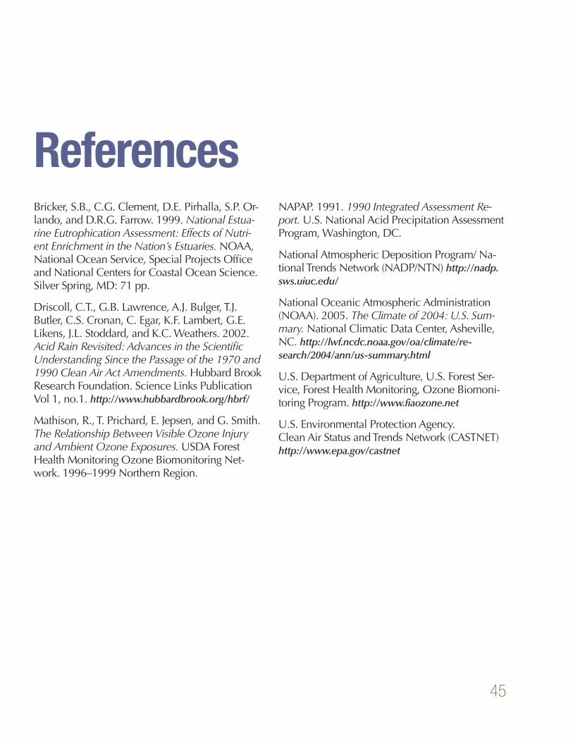
ReferencesBricker, S.B., C.G. Clement, D.E. Pirhalla, S.P. Or-lando, and D.R.G. Farrow. 1999. National Estua-rine Eutrophication Assessment: Effects of Nutri-ent Enrichment in the Nation’s Estuaries. NOAA, National Ocean Service, Special Projects Office and National Centers for Coastal Ocean Science. Silver Spring, MD: 71 pp.

Driscoll, C.T., G.B. Lawrence, A.J. Bulger, T.J. Butler, C.S. Cronan, C. Egar, K.F. Lambert, G.E. Likens, J.L. Stoddard, and K.C. Weathers. 2002. Acid Rain Revisited: Advances in the Scientific Understanding Since the Passage of the 1970 and 1990 Clean Air Act Amendments. Hubbard Brook Research Foundation. Science Links Publication Vol 1, no.1. http://www.hubbardbrook.org/hbrf/

Mathison, R., T. Prichard, E. Jepsen, and G. Smith. The Relationship Between Visible Ozone Injury and Ambient Ozone Exposures. USDA Forest Health Monitoring Ozone Biomonitoring Net-work. 1996–1999 Northern Region.

NAPAP. 1991. 1990 Integrated Assessment Re-port. U.S. National Acid Precipitation Assessment Program, Washington, DC.

National Atmospheric Deposition Program/ Na-tional Trends Network (NADP/NTN) http://nadp.sws.uiuc.edu/

National Oceanic Atmospheric Administration (NOAA). 2005. The Climate of 2004: U.S. Sum-mary. National Climatic Data Center, Asheville, NC. http://lwf.ncdc.noaa.gov/oa/climate/re-search/2004/ann/us-summary.html

U.S. Department of Agriculture, U.S. Forest Ser-vice, Forest Health Monitoring, Ozone Biomoni-toring Program. http://www.fiaozone.net

U.S. Environmental Protection Agency. Clean Air Status and Trends Network (CASTNET) http://www.epa.gov/castnet

46

Clean Air Markets DivisionOffice of Air and Radiation

U.S. Environmental Protection Agency1200 Pennsylvania Avenue, NW (6204J)Washington, D.C. 20460

EPA 430-R-05-007www.epa.gov/airmarkets

October 2005

Recycled/Recyclable. Printed with Vegetable Oil-Based Inks on Recycled Paper (Minimum 50% Postconsumer) Process Chlorine Free