Draft version September 4, 2014Preprint typeset using LATEX style emulateapj v. 5/2/11

THE PANCHROMATIC HUBBLE ANDROMEDA TREASURY X. ULTRAVIOLET TO INFRAREDPHOTOMETRY OF 117 MILLION EQUIDISTANT STARS

Benjamin F. Williams1, Dustin Lang2, Julianne J. Dalcanton1, Andrew E. Dolphin3, Daniel R. Weisz1,4,5,Eric F. Bell6, Luciana Bianchi7, Eleanor Byler1, Karoline M. Gilbert8, Leo Girardi9, Karl Gordon8,

Dylan Gregersen10, L. C. Johnson1, Jason Kalirai7,8, Tod R. Lauer11, Antonela Monachesi6, PhilipRosenfield12, Anil Seth10, and Evan Skillman13

Draft version September 4, 2014

ABSTRACT

We have measured stellar photometry with the Hubble Space Telescope (HST) Wide Field Cam-era 3 (WFC3) and Advanced Camera for Surveys (ACS) in near ultraviolet (F275W, F336W),optical (F475W, F814W), and near infrared (F110W, F160W) bands for 117 million resolvedstars in M31. As part of the Panchromatic Hubble Andromeda Treasury (PHAT) survey, wemeasured photometry with simultaneous point spread function fitting across all bands and atall source positions after precise astrometric image alignment (<5-10 milliarcsecond accuracy).In the outer disk, the photometry reaches a completeness-limited depth of F475W∼28, while inthe crowded, high surface brightness bulge, the photometry reaches F475W∼25. We find thatsimultaneous photometry and optimized measurement parameters significantly increase the de-tection limit of the lowest resolution filters (WFC3/IR) providing color-magnitude diagrams thatare up to 2.5 magnitudes deeper when compared with color-magnitude diagrams from WFC3/IRphotometry alone. We present extensive analysis of the data quality including comparisons ofluminosity functions and repeat measurements, and we use artificial star tests to quantify pho-tometric completeness, uncertainties and biases. We find that largest sources of systematic errorin the photometry are due to spatial variations in the point spread function models and chargetransfer efficiency corrections. This stellar catalog is the largest ever produced for equidistantsources, and is publicly available for download by the community.

1. INTRODUCTION

The stellar content of galaxies probes fundamentalquantities such as the initial mass function, the clus-ter mass function, the distance scale, stellar evolution,

1 Department of Astronomy, Box 351580, University ofWashington, Seattle, WA 98195; ben@astro.washington.edu,jd@astro.washington.edu, byler@astro.washington.edu,lcjohnso@astro.washington.edu,

2 McWilliams Center for Cosmology, Department ofPhysics, Carnegie Mellon University, 5000 Forbes Ave.,Pittsburgh, PA; dstn@cmu.edu

3 Raytheon, 1151 E. Hermans Road, Tucson, AZ 85706;adolphin@raytheon.com

4 Department of Astronomy, University of Californiaat Santa Cruz,1156 High Street, Santa Cruz, CA, 95064;drw@ucsc.edu

5 Hubble Fellow6 Department of Astronomy, University of Michigan,

830 Denninson Building, Ann Arbor, MI 48109-1042; an-tonela@umich.edu,ericbell@umich.edu

7 Department of Physics and Astronomy, Johns HopkinsUniversity, 3400 North Charles Street, Baltimore, MD 21218;bianchi@pha.jhu.edu

8 Space Telescope Science Institute, Baltimore, MD 21218;kgilbert@stsci.edu, kgordon@stsci.edu, jkalirai@stsci.edu

9 Osservatorio Astronomico di Padova – INAF,Vicolo dell’Osservatorio 5, I-35122 Padova, Italy,leo.girardi@oapd.inaf.it

10 Department of Astronomy, University of Utah; dy-lan.gregersen@utah.edu, aseth@astro.utah.edu

11 NOAO, 950 North Cherry Avenue, Tucson, AZ 85721;lauer@noao.edu

12 Dipartimento di Fisica e Astronomia Galileo Galilei,Universita di Padova, Vicolo dell’Osservatorio 3, I-35122Padova, Italy

13 Department of Astronomy, University of Minnesota, 116Church SE, Minneapolis, MN 55455; skillman@astro.umn.edu

galaxy growth, the history of star formation, and starformation feedback energetics. Resolved stellar pho-tometry for a massive spiral galaxy therefore providesa superb testbed for validating the details of many as-trophysical processes.

Interpreting large libraries of Galactic stars is cur-rently challenging due to the uncertain and wide-ranging distances and extinctions. In contrast, M31,the nearest large spiral galaxy to our own, is far enoughaway that all of the disk stars are at the same distanceto within ∼1%. Furthermore, M31 is the only othergalaxy in the Local Group that is similar in mass, mor-phology, and metallicity to those that host most of thestellar content of the universe (massive disk-dominatedgalaxies of roughly solar metallicity; Driver et al. 2007;Gallazzi et al. 2008).

1.1. Ground-based M31 Disk Catalogs

Although M31 seems an ideal target for producinga valuable library of stellar photometry, work has his-torically been inhibited by its large angular size (190′

major axis; de Vaucouleurs et al. 1991). Most groundbased studies of M31 that have concentrated on thefield star population, on OB associations, or on por-tions of the halo (Massey et al. 1986; Mould & Kris-tian 1986; Pritchet & van den Bergh 1988; Haimanet al. 1994; Davidge 1993; Durrell et al. 1994, 2001;Ibata et al. 2001; McConnachie et al. 2009).

Due to the poor angular resolution available, ground-based surveys of the disk are limited to photometry ofonly the brightest stars. The first resolved star studycovering the optical disk was that of Magnier et al.

arX

iv:1

409.

0899

v1 [

astr

o-ph

.GA

] 2

Sep

201

4

2

(1992), providing a catalog of 360,000 objects in 4bands. This catalog has been superseded by Masseyet al. (2006), which contains a similar number of starsin 5 bands with improved photometric and astrometricprecision and which has led to a census of the bright-est and most massive M31 members. This photometryalso provided some constraints on the age distributionand star formation rate of the disk (Williams 2003).

Ground-based halo studies have taken advantage ofthe very large fields of view available on many tele-scopes, leading to the discovery of extended densityfeatures from accreted smaller galaxies (Ibata et al.2001; Ferguson et al. 2002). Further ground-based pho-tometry and spectral work showed the halo metallicitygradient and more structure (McConnachie et al. 2009;Gilbert et al. 2012).

1.2. HST M31 Catalogs

Until now, HST imaging has been limited in cover-age because of the large angular size of M31; however,even small studies have had significant scientific im-pact. Studies of the stellar populations in the bulge inthe UV (Bertola et al. 1995) resolved hot stars, laterfound to be post-AGB stars (Brown et al. 2008). Stud-ies of the luminosity function of the field stars in thebulge have also been done in the IR (Stephens et al.2003).

HST observations of the resolved stellar populationsof halo fields provided detailed evidence of its metal-rich nature (Rich et al. 1996), and very deep obser-vations have provided the detailed metallicity and agedistribution of a handful of halo pointings (Brown et al.2003, 2006, 2007, 2008, 2009)

There have been several isolated HST fields in thedisk analyzed as well (Sarajedini & Van Duyne 2001;Williams 2002; Bellazzini et al. 2003; Ferguson et al.2005; Brown et al. 2006). These studies have providedinsight into how portions of the disk formed, includ-ing finding signs for early metal enrichment, a typicalage older than 1 Gyr and extended star formation inmany of the currently star forming regions. Further-more, many individual star forming regions in the diskhave been observed in detail in the UV (e.g., Bianchiet al. 2012), allowing initial measurements of hierarchi-cal clustering and dispersion timescales of young stars.

Many other HST resolved star studies of M31 havefocused on star clusters, measuring metallicities, struc-tural parameters for old clusters (e.g., Holland et al.1997; Barmby et al. 2000, 2002) and ages for youngclusters (Williams & Hodge 2001a,b), finding manysimilarities to the Milky Way cluster population, buta larger number of young, massive clusters in M31.Improved catalogs and measurements of star clusterparameters have also been ongoing (Krienke & Hodge2008; Barmby et al. 2009; Hodge et al. 2010; Perinaet al. 2010; Tanvir et al. 2012; Wang & Ma 2013; Agar& Barmby 2013)

All of these studies to date made significant advancesin our knowledge of M31, even though they were lim-ited to scattered fields across the disk and halo of M31.

1.3. The Panchromatic Hubble Andromeda Treasury

Given that M31 offers the best opportunity to studythe resolved stellar populations of a large spiral galaxy,

we carried out the Panchromatic Hubble AndromedaTreasury (PHAT) survey, covering ∼1/3 of the star-forming disk of M31 in six bands from the near-UV tothe near-IR using HST’s imaging cameras. This sur-vey combines the wide field coverage typical of ground-based surveys with the precision of HST observations.The overall survey strategy, initial photometry anddata quality assessments were described in detail inDalcanton et al. (2012a). Our wavelength coverageprovides the data necessary to constrain masses, metal-licities, and extinctions of individual stars, from whichwe can infer the spatially-resolved metallicity, age, andextinction distributions over a very large contiguousarea.

The PHAT survey has been instrumental in severalM31 discoveries already. These include improved con-straints on post-AGB and AGB-manque evolutionaryphases (Rosenfield et al. 2012), tracing the stellar massdistribution of the inner M31 halo (Williams et al.2012), new techniques for measuring robust ages andmasses of star clusters (Beerman et al. 2012) and formeasuring the initial mass function from resolved stel-lar photometry (Weisz et al. 2013), a major increasein the number of cataloged star clusters in M31 (John-son et al. 2012; Fouesneau et al. 2014), evidence for ametallicity ceiling for Carbon stars (Boyer et al. 2013),and additional complexity in the structural compo-nents of M31 (Dorman et al. 2013). These results werebased on our first generation of photometry, wheremeasurements were made for each camera separately,and then combined at the catalog level.

In this paper, we report on our second generationof photometric measurements of the resolved stars inthe PHAT imaging, in which we take advantage of allavailable information by carrying out photometry si-multaneously in all 6 filters. This new approach givesa significant increase in the depth and accuracy of ourphotometry over that presented in Dalcanton et al.(2012a). Section 2 describes our technique for per-forming and merging simultaneous 6-filter photome-try, fitting data from 3 HST cameras with differentpoint spread functions (PSFs), distortion corrections,and pixel scales. Section 3 details the resulting color-magnitude diagrams (CMDs). Section 4 discusses con-tamination from non-M31 sources. Section 5 gives thedetailed analysis of the quality of the photometry, in-cluding a full assessment of random and systematicuncertainties. Section 6 compares this generation ofPHAT photometry to the previous version. Section 7describes individual fields whose photometry may dif-fer from that of the survey in general. Section 8 de-scribes the available data products. Finally, Section 9provides a summary of our work.

2. DATA

2.1. Survey Overview

The data for the PHAT survey were obtained fromJuly 12, 2010 to October 12, 2013 using the Ad-vanced Camera for Surveys (ACS) Wide Field Chan-nel (WFC), the Wide Field Camera 3 (WFC3) IR(infrared) channel, and the WFC3 UVIS (Ultraviolet-Optical) channel. The observing strategy is describedin detail in Dalcanton et al. (2012a). In brief, we per-

3

formed 414 2-orbit visits. Each visit was matched byanother visit with the telescope rotated at 180 degrees,so that each location in the survey footprint was cov-ered by the WFC3/IR, WFC3/UVIS, and ACS/WFCcameras. The different orientations were schedulable6 months apart from one another, so that the WFC3data and ACS observations of each region were sep-arated by 6 months. A list of the target names, ob-serving dates, coordinates, orientations, instruments,exposure times, and filters is given in Table 1. Wenote that each field includes a short (<20 sec) expo-sure in F475W and F814W to avoid saturation of thebrightest stars. In total, the area covered by all 6 filtersis 0.5 deg2.

The survey was designed around the camera with thesmallest footprint, the WFC3/IR. Thus the tiling ismost easily navigated by plotting the WFC3/IR foot-prints, as shown in the F160W exposure map in Fig-ure 2. The area plotted in Figure 2 corresponds toa single rectangle in Figure 1. The ACS/WFC andWFC3/UVIS exposure maps are shown in Figure 3.This tiling was necessarily much more complex to max-imize the contiguous WFC3/IR coverage and make themost efficient use of the ACS parallels.

Each survey region is described by two identifiers,a “brick” number and a “field” number. “Bricks” arerectangular areas of ∼6′×12′ that correspond to a 3×6array of WFC3/IR footprints. The bricks are num-bered, 1-23, starting from the brick at the nucleus,and counting west to east, south to north. Odd num-bered bricks move out along M31’s major axis, andeven numbered bricks follow the eastern side of theodd-numbered bricks, as shown in Figure 1. Withineach of the 23 bricks, there are 18 “fields” that eachcorrespond to an IR footprint. These fields are num-bered, 1-18, from the northeast corner, counting eastto west, north to south (see Figure 2). Thus, Brick 23-Field 18 is the IR footprint in the southwest cornerof the brick farthest out along the major axis. Eachpointing has its own unique brick, field number. Im-ages in other cameras are labeled by the brick and fieldof the IR footprint they primarily overlap (e.g., M31-B01-F13-ACS overlaps M31-B01-F13-IR even thoughit was taken in parallel during the primary observa-tions of M31-B01-F16-IR).

Although the neighboring fields overlap significantlyin ACS and UVIS, for the purposes of this generationof photometry, we were not able to take advantage ofthis extra exposure due to computational limitations.Including all exposures that overlap a location in oursurvey requires putting more than 200 CCD reads intomemory and slows down the measurements, requiringa large amount of processing time on expensive high-memory machines. Therefore, when carrying out the6-filter photometry for each survey brick+field, we in-cluded only the UVIS, ACS, and IR data specificallypointed at that brick+field. The effective exposure foreach field as measured is shown in Figure 4. Note thatthe single-field data leaves the chip gap in ACS uncov-ered; we discuss how these areas were treated in Sec-tion 2.4. The Figure also shows the other exposuresin the survey that could be included in the photom-etry of this single field. For our next generation ofphotometry, the computing power should be available

to include all overlapping exposures when measuringphotometry of each field, which will improve the depthand homogeneity of the photometry.

2.2. Astrometry

To measure stars in all 6 bands, our first challengewas to align all of our data to a relative precision of∼0.1 ACS pixel (5 milliarcseconds). We aligned theimages based on preliminary star catalogs using ini-tial photometry performed on each individual CCDreadout to generate initial positions of stars for eachCCD of each exposure. These catalogs were then cross-correlated to solve for the relative astrometry of eachCCD of each exposure in each brick. We now describethe process in detail.

We first cleaned the images of cosmic rays (CRs) toavoid them being mistakenly matched and hinderingalignment. The flt images as initially downloadedfrom MAST at the time did not have well-determinedCRs, partially due to our observing strategy, whichhad only 2 exposures per band in UVIS and a verywide range of exposure times in ACS. Therefore, weperformed out own CR flagging with the PyRAF taskastrodrizzle (Gonzaga 2012), which identifies CRs byfinding pixels that are bright in one exposure and notin the other exposures in the same band. The CRswere identified and flagged in the DQ extensions of theflt images. We note that the MAST data reductionpipeline is always improving, so that future downloadsmay not require this extra step for reliable CR flagging.

We used the point spread function photometry pack-age DOLPHOT — an updated version of HSTPHOT(Dolphin 2000) — to find and measure the positionsof stars on each CCD of each exposure of the survey.These positions provide the basis for astrometric align-ment. The DOLPHOT task acsmask or wfc3mask up-dates the images into units of counts per pixel appro-priate for DOLPHOT photometry. This task appliesthe data quality (DQ) flags as well as the pixel areamap to the flt science (SCI) extensions to mask outbad pixels and CRs, and calibrates the flux in eachpixel by the area coverage on the sky. The flt im-ages were then split into their individual CCDs usingthe DOLPHOT task splitgroups. These single-CCDDOLPHOT catalogs were culled for artifacts using thesame criteria as those used for the single-camera pho-tometry in Dalcanton et al. (2012a).

For the UVIS and short ACS exposures, in somecases there were fewer than ∼10 stars for determin-ing alignment. For several of these cases, we foundthat alignment solutions were not acceptable when wemeasured star positions on the flat-fielded (flt) im-ages. However, we circumvented this problem in manycases by measuring star positions on charge transfer ef-ficiency (CTE)-corrected (flc) images in cases whereconvergence was not reached from the positions mea-sured on the flt images. Thus, we found that theCTE-corrected images produce more reliable centroidsthan the flt images, showing the high-quality of theon-image CTE-correction algorithm (Anderson & Be-din 2010). However, there were still some exposuresthat were not able to be aligned due to the low densityof detected point sources (see Section7).

Using the single-CCD catalogs, astrometric align-

4

ment was performed as follows. We first aligned theACS catalogs with exposure times > 30 seconds witheach other and with a deep CFHT i-band image (whichwas in turn calibrated to 2MASS). The alignment pro-ceeds by assuming the input astrometry is roughly cor-rect and then performing an astrometric cross-matchbetween each pair of ACS images and each ACS imageto the CFHT reference catalog. We align the bright-est stars in each sample to reduce the computationalcost and to reduce the impact of measurement errorin fainter stars. Each matching provides a set of as-trometric offsets, some of which are correct and someof which are due to spurious matches, or matches toneighboring stars. We fit these offsets as a mixture ofa flat background (for spurious matches) and a Gaus-sian (for correct matches), using a coarse histogram toinitialize an Expectation-Maximization method. Theresult allows us to weight each matched star by itsprobability of being drawn from the foreground distri-bution. We then solve the large least-squares problemto find astrometric shifts and affine transforms (rota-tions, scalings, and shears) of each input catalog tominimize the matching residuals. We repeat this pro-cess several times, using a decreasing matching radiusand including an increasing number of fainter stars.After having aligned the long ACS exposures with eachother and the reference frame in this way, we repeatthis process, aligning the short ACS exposures and theWFC3 IR and UVIS exposures to the ACS reference.

The result of these alignment processes is a setof scripts that update the FITS WCS astrometricheaders of the input images, including all affinegeometric transformations. We applied the imageheader update scripts to their respective flt imagesas originally downloaded from STScI and processedby OPUS 2012 4. We then combined images withupdated astrometry to produce images of each brick ineach band, using the PyRAF task astrodrizzle withthe following altered parameters: context=True,build=True, skysub=False, final wcs=True,final rot=0.0, clean=True. These brickwideastrodrizzled images are available from the SpaceTelescope Science Institute through the high-levelscience products archive.

A zoomed example of a small (17′′×17′′) regionwith many overlaps in all 3 cameras is shown in Fig-ure 5, which reveals the seamless nature of our stacked,aligned data. More quantitative alignment checks areshown in Figure 6, where the first 3 panels show er-ror ellipses are plotted for each individual CCD readcompared to the reference frame (gray), to other CCDreads in the same filter (red), and compared to CCDreads in other filters (blue). These one-sigma error el-lipses were measured via expectation-maximization ofa model of all star-to-star matches between each pair ofexposures. The alignment uncertainties were typically<∼ 0.01′′ between different HST images in all cameras.

The reference frame is the ground-based global astro-metric reference for F475W, and the F475W imagesprovide the reference frame for the other bands. Theuncertainties on the alignment between the F475Wand the reference frame are the largest (though still∼0.05′′).

The resulting images were carefully checked by eye

to look for any problems with alignments within eachfield and across overlaps with neighboring fields. Thesebrickwide images are also publicly released in theMikulski Archive at Space Telescope (MAST) HighLevel Science Products (HLSP).

2.3. Data Processing

After updating the original flt images with new as-trometry, the images were passed through our multi-camera photometry pipeline, which consists of severalpre-processing steps, the run of DOLPHOT, and sev-eral post-processing steps to check quality and produceeasy-to-use data products. We now describe the stepsin detail.

2.3.1. Running DOLPHOT

The preprocessing divides the data into differentgroups determined by their respective brick+field lo-cations. Data from each brick+field were processedseparately (see left panel of Figure 4). This stack con-tains 31 CCD reads. There are 9 ACS exposures (2CCDs per exposure), 5 IR exposures (1 CCD per ex-posure), and 4 UVIS exposures (2 CCDs per exposure).Thus, there were 18 separate groups of 31 CCD readsfor each brick. The entire processing pipeline was runindependently for each of these 18 groups.

Within each group, all of the preprocessing of theindividual images was carried out in the same man-ner as when preparing them for individual photome-try (see previous subsection), but with improved align-ment. The identification of CRs was also more reliablebecause prior to our astrometry updates, misalignedstars were sometimes identified as CRs.

DOLPHOT uses a reference image as the astromet-ric standard. It ties each detection to a location onthe reference image. We used the stacked, distortion-corrected F475W image as this reference because it of-fers the best combination of depth, completeness, andresolution. To generate the F475W reference image,the F475W astrodrizzle output was also processed withacsmask, calcsky, and splitgroups in order to be usedas the DOLPHOT reference image.

As described in Dalcanton et al. (2012a), the pack-age DOLPHOT was used for all of the photometry forthe PHAT survey. However, the quality of the pho-tometry output from DOLPHOT is strongly depen-dent on the appropriateness of the parameters set bythe user. In particular, the precision and complete-ness of photometry in very crowded fields—like thosein the PHAT survey—can be strongly affected by thetechnique DOLPHOT uses to measure the local skyand the size of the aperture used for determining PSFoffsets.

To optimize our photometry, we performed a grid oftest runs of DOLPHOT on several select fields usinga variety of DOLPHOT parameters. The parameterswe varied were RAper, RChi, FitSky, and PSFPhot whichcontrol the radius inside of which aperture photome-try is compared with PSF-fitting, the radius inside ofwhich the quality of the PSF fit is assessed, the methodfor measuring the background level for each star, andthe weighting during PSF fitting, respectively. Rangesof the parameters were 2–8, 1.5–8, 1–3, and 1–2 for

5

each of the four parameters, respectively. One thou-sand artificial stars were inserted at each of 2–3 CMDlocations roughly corresponding to the main sequence(UVIS and ACS only), the RGB (ACS and IR only),and ∼1 mag above the S/N cutoff in both filters (all3 cameras). All of our photometry uses the Anderson(ACS ISR 2006-01) PSF library.

To assess the quality of each set of test parameters,we calculated the number of detected sources (all 3cameras), the red clump tightness (ACS only), andthe RGB width (IR only) as measured from the outputphotometry for all combinations of processing parame-ters. We also assessed the artificial star completeness,bias, and scatter (all 3 cameras) as measured from theartificial star tests performed on the test fields for eachset of test parameters.

Based on these metrics, the best photometry re-sulted from small apertures, standard PSF photomet-ric weighting, and measuring the sky immediately out-side the photometry aperture (but within the PSF).This requires adjusting the PSF for the fact that skyis being measured in a region where the star itself con-tributes. These parameters were clearly superior inthe most crowded regions, and were at least as goodas other parameter combinations in uncrowded regions,where the sensitivity to parameter choices is much less.Our final DOLPHOT processing parameters are givenin Table 2.

We note that while CTE correction was turned on(UseCTE=1), CTE corrections were only made for theACS bands (F475W and F814W) because when we be-gan our photometry no CTE corrections were availablefor WFC3. In the next generation of photometry, weplan to run our measurements on CTE-corrected im-ages, and turn the DOLPHOT CTE corrections off,which may further improve the level of systematic er-rors in our photometry.

We were able to improve the results from DOLPHOTby fixing the ref2img parameters, which control thedistortion terms for the aligning images. To optimizecross-camera alignment, DOLPHOT uses the manystars in the image stack to refine the distortion so-lution for each camera. If these parameters were al-lowed to be freely fitted for all individual fields, some-times relatively empty short exposures or UV expo-sures could throw off the solution. Thus, using a fewfields from Brick 21, where the crowding is low, and thedensity of UV-bright stars is relatively high, we mea-sured the ref2img values that provided the best imagealignment. This DOLPHOT parameter provides minorchanges to the IDCTAB specified distortions, whichyield the best fit for our data, but because we did notinclude the overlaps at different cross-camera orienta-tions from the standard PHAT observation strategy,our precise terms would likely not be relevant for otherHST observing programs.

We fixed the ref2img values measured in Brick 21 forthe rest of the survey data, which resulted in excellentalignment across the survey. DOLPHOT measures theprecision by which the images of the input stack arealigned with the reference image. Our median astro-metric precision is ∼5 milliarcseconds. In the lower-right panel of Figure 6, we provide the histogram ofalignment values from DOLPHOT, in units of pixels,

for all of the CCD chip readouts for the entire survey,showing 99.8% of all of the survey images are aligned to0.5 pixels or better. The median value is 0.11 ACS pix-els, or 5 milliarcseconds. The small tail of CCD readswith poor alignment are a small fraction of the veryshort exposure (10–15 s) ACS images in regions withfew bright stars, and a few UVIS exposures in regionsalong the NE edge of the survey with little or no youngstars to align the image. These few images are essen-tially pure noise, and therefore contribute very little toany of our photometry measurements. Because few, ifany, stars are detected in these exposures, they are notincluded in the vast majority of combined photometrymeasurements. In cases where a noise spike is mea-sured in the very short optical exposures (i.e. any starnot saturated in the long exposures), that measure-ment will be weighted at 0.006 (0.6%, the fraction ofthe exposure time in these frames), making its effectson the resulting photometry at most 0.6%. These fieldsare described in more detail, along the other fields thathave data issues, in § 7.

When DOLPHOT is run on a collection of images,all of the individual CCDs are aligned to the referenceimage in memory, stacked to search for any significantpeaks, and then each significant peak above the back-ground level is fitted with the point spread function forthe specific band, and camera of each CCD in the stack.The measurements are corrected for charge transfer ef-ficiency (CTE, ACS only) and calibrated to infiniteaperture. The measurements are then combined into afinal measurement of the photometry of the star. Thefinal measurements include a combined value for alldata in each band for the count rate, rate error, VEGAmagnitude and error, background, χ of the PSF fit,sharpness, roundness, crowding, and signal-to-noise.

VEGA magnitudes apply the encircled energy cor-rections and zero points from the ACS handbook dated15-July-2008 and the WFC3 encircled energy correc-tions and zero points from 2010 by J. Kalirai. Therate and rate error measurements are particularly use-ful for stars that were not detected in one or morebands (and therefore have negative rates or rates of 0,which results in an undefined magnitude), as they pro-vide upper-limits in these bands that can be employedfor constraints when fitting spectral energy distribu-tions. The sharpness is zero for a perfectly-fit star,positive for a star that is too sharp (perhaps a cosmicray), and negative for a star that is too broad (per-haps a blend, cluster, or galaxy). The crowding pa-rameter is in magnitudes, and tells how much brighterthe star would have been measured had nearby starsnot been fit simultaneously. For an isolated star, thevalue is zero. These measurements are also output foreach individual exposure, allowing for the possibility ofvariability studies (Wagner-Kaiser et al., in prep.) orsearches for artifacts not masked by our preprocessingtechniques. All measurements are output to a “.phot”ascii file.

2.3.2. Creation of Photometry Catalogs

The star positions from DOLPHOT are then con-verted to RA and Dec using the header of the refer-ence image (see above) for astrometry. RA and Decare then added to the phot catalog, and the full pho-

6

tometric catalog (481 columns) is placed into a taggedFITS table (.phot.fits file). The data are then culledto include only the combined output for sources, sig-nificantly reducing the size of the data files for thosenot interested in the measurements on the individualCCD chips. At this step, we also kept only sourceswith S/N≥4 and reasonable sharpness (see Table 3) inat least one band (“ST” catalogs) to limit the numberof noise spikes, CRs, and artifacts surrounding satu-rated stars in our catalogs. This initial cut removedup to 20% of the objects from the initial DOLPHOToutput, mostly very low signal-to-noise with some scat-tered brighter measurements. An example CMD of theculled objects is shown in the right side panel of Fig-ure 7, and it shows no overdensities associated withtypical CMD features. Thus, users looking for a spe-cific source may find it in the pre-culled phot.fitsfiles, if it is not contained in the ST files; however, anymeasurement not included in the ST files should onlybe used with extreme caution.

The sources in the ST catalog are then flagged sothat any band with measurements of high crowding orhigh square of the sharpness (see Table 3) or that haveS/N<4 can be easily left out of any analysis, result-ing in the “GST” sample. The flagged measurementsare likely to be unreliable (strongly affected by blend-ing, CRs, or instrument artifacts). The key differencebetween all measurements in the ST catalogs and thesubset that pass our GST criteria is that the GST cri-teria are performed per band. For example, if a staris well-measured in F275W, F336W, F475W, F814W,and F110W it may not be well-measured in F160W.Measurements in all six bands for the star will appearin the catalog, but its F160W measurement will havea GST flag of 0. A further difference between the fullcatalog measurements and those with the GST flag isthe use of crowding as a quality metric. Crowding isone of the quality metrics considered when determiningwhich bands pass the GST flag criteria for each star;however, crowding is not considered at all for inclusionin ST the catalog.

The precise values of sharpness and crowding usedfor cutting were different for the UV, optical, and IR,and are provided in Table 3. We used both qualitativeand quantitative criteria to determine the photomet-ric quality cuts that maximize the quality of the stel-lar CMDs (e.g., number of stars, photometric depth,tightness of features) and minimize the number of non-stellar objects (e.g., blends, background galaxies, cos-mic rays). We accomplished this by a combination ofvisual inspection and fitting particular CMDs, whichwe now describe.

For each permutation of DOLPHOT input parame-ters (raper, rchi, fit sky psfphot), we constructed140 per-camera CMDs for various permutations ofsharpness and crowding. For each CMD, we calcu-lated or visually inspected the following factors: CMDdepth for a fixed SNR=4, number of stars that passedthe photometric cuts, quality of maximum likelihoodfits of a Gaussian plus line model to the color and lu-minosity profile of the RC (only for the ACS and IRCMDs), and the CMD of rejected objects. In addi-tion, we also considered the completeness fraction andcolor/magnitude biases from sets of artificial star tests

(ASTs). Specifically, for each CMD, we inserted 1000ASTs 1 magnitude above the S/N limit, 1000 on theupper MS, and 1000 on the upper RGB. We computedthe recovered fraction (i.e., completeness) and meanmagnitude and color biases for each set of 1000 ASTs.

Using all of the above criteria, we found that themajority of photometric quality cut combinations pro-duced CMDs that were clearly not ideal (e.g., poorcompleteness, obvious stellar features on the rejectedCMDs, poor fits to the RC). We readily eliminatedthese permutations and focused on the small subsetthat produced deep CMDs with clear features. Todistinguish among these, we primarily considered thecompleteness fraction and magnitude and color spreadsof the AST sets. We also visually compared high S/Nregions of the various CMDs for tightness of the lu-minous CMD features (e.g., upper MS), and elimi-nated those that rejected a higher percentage of highS/N objects that had colors and magnitudes consistentwith known stellar sequences (e.g., MS, HeB sequence).Based on this iterative process, we found the param-eters listed in Table 3 provided for the best overallCMDs. We note that these cuts were chosen to providean approximate set of values for obtaining high-qualityCMDs from our catalogs over the entire survey. Thoseusing our photometry for specific projects will likelywant to determine their own flags optimized for theirscience needs.

2.4. Merging Catalogs

The final ST photometry catalogs for the individ-ual fields are then combined into brick-wide catalogs,and then into a survey-wide catalog. To avoid du-plicate catalog entries, for each brick we generated agrid in RA and Dec with single-point corners insidethe IR footprint corners of the survey, creating uniqueregions and trimming the IR detector edges simultane-ously. Then the catalog of each field of the grid wascut to include only detections inside of that field re-gion as defined by the grid. These cut catalogs werethen combined into a initial brickwide catalogs with noduplicate entries and no gaps in UVIS or IR coverage.

Because ACS exposures from neighboring fields arenot included in the DOLPHOT photometry measure-ments of an individual field, the ACS chip gap containsno optical coverage (the UVIS chip gap was coveredby dithers). Thus, the initial brickwide catalogs hadonly UV and IR measurements for stars in the ACSchip gap. However, the catalogs for the neighboringfields contain optical measurements at these locations.Within the chip gaps, we include ACS measurementsfrom neighboring fields: for example, the top half ofthe chip gap in Field 1 is has optical measurements inthe catalog for Field 2 (the field to the right), while thebottom half has optical measurements in the catalogfor Field 7 (the field below). The resulting final brick-wide catalogs have full 6-band coverage throughout,although the photometry in the chip gap has matchingthat was performed at the catalog level. Therefore, inthe ACS chip gaps, the UVIS and IR photometry willbe of different quality due to the lack of ACS data inthat region when the image stack was being reduced(see Section 6). To allow investigators to efficientlyleave out the chip gaps if they would like to avoid

7

these non-uniform measurements, we have included aninside chipgap flag in our catalogs, which is set to1 for all stars that were affected by this catalog-levelmerging.

We defined brick edges in the same way as field edges,with single corner points. Then we trimmed the brick-wide catalogs to contain only stars within these singlecorner points. Once trimmed in this way, the catalogscould be merged to produce a single catalog for theentire survey with no duplicate entries and no gaps in6-band coverage. We note the only gap to be the 0.1arcmin2 area that we did not observe due to changesin the observing program that were necessary to haveguide stars for all observations (see Section 7.3 for de-tails).

The number of stars in each 6-band brick catalogis given in Table 4, where the total number of STstars measured in each brick is given along with thenumber of reliable (high signal-to-noise, low crowding)GST measurements in each band. The entire genera-tion 2 catalog has 116,861,772 stars. Each one of thesewas measured in at least 16 exposures (ignoring over-laps between fields and the very short ACS exposures),making 1,869,788,352 photometric measurements. Incases where the star was not detected in a given band,the rate and rate error, measured based on the skylevel, can be used as a constraint for a non-detection,which is recorded as a 99.999 in the magnitude column.The full catalog is available in machine readable formaton Vizier. The individual brick catalogs are availablein FITS format from MAST.14 A small example of thecatalog is provided in Table 5.

It is clear from Table 4 that no band has good mea-surements of all 117 million stars, but each of the 117million stars has a good measurement in at least oneband. The most extreme cases of this are in the UV,where only 0.3% of the total 2nd generation cataloghas reliable measurements (other than upper-limits)for both the F275W and F336W bands. A very highpercentage of these UV measurements are actually full6-band measurements.

In Figure 8 we plot UV, Optical, and IR CMDs of asmall random sample from our catalog, with the pointscolor-coded by the total number of bands with reliablemeasurements. The UV CMD shows that nearly everydata point corresponds to a star with reliable measure-ments in all 6 bands. The optical CMD shows that ahigh fraction of RGB stars are detected in 4 bands(the optical and IR bands), and only the brightestmain-sequence stars tend to be detected in 6 bands.The IR CMD shows again that most RGB stars aremeasured in 4 bands (optical and IR) while only thebrightest main sequence stars are measured in the UV.Taken together, these results show that only faint bluestars tend to have good measurements in fewer than4 bands. UV-bright stars tend to have good IR mea-surements, but IR-bright stars do not tend to havegood UV measurements. Both tend to have good op-tical measurements, given that the ACS data have thegreatest depth in terms of CMD features; however, thereddest RGB stars are only detected in the IR.

14 http://archive.stsci.edu/missions/hlsp/phat/

3. CMDS

We show the UV photometry for the entire surveyin the CMDs in Figure 9. The UV photometry hadroughly equal depth throughout the survey because ithad constant, low crowding everywhere due to its notbeing deep enough to include the very numerous RGBstars, which are very faint in the UV. Thus, only forthe UV do we show the entire survey on a single CMD.The figure shows the CMD before our quality cuts,the fraction of sources that pass our quality cuts as afunction of color and magnitude, and the CMD afterour quality cuts. Stars that survive the cuts but fall inregions where large fractions of the stars were rejectedhave a higher probability of being poor measurements.

Because of the high density of RGB stars in M31, thedepth of our optical and IR photometry varied greatlywith position in the galaxy. We therefore have pro-duced 6 color-magnitude diagrams in each of 4 filtercombinations, following the spatial distribution shownin Figure 10. These densities are relative logarithmicstar number densities taken from a model distribution.They were used only to provide a reasonable divisionof the catalog into regions with similar photometricdepths. The areal coverage of each stellar densityrange is different, with 770, 481, 349, 113, 106, and31 arcmin2 for the 0.0–0.3, 0.3–0.6, 0.6–1.2, 1.2–1.8,1.8–3.0 and 3.0–8.0 regions, respectively. In figures 11-18, we show the fraction of measurements that pass ourquality cuts, and the CMDs after quality cuts in eachof these filter combinations at each of these densities.

Apart from the familiar features like the RGB andmain sequence, these CMDs reveal several detailed fea-tures that have been already commented on in Dalcan-ton et al. (2012a, Figure 20), but which appear some-what more clearly in the present photometry, such asthe sharp drop in star counts at the tip of the RGB atF814W∼20 or F160W∼18, and spanning a broad rangeof colors, the red clump at F814W∼24 or F160W∼23.5.Other features appear that are associated with the redclump, such as the extension to red colors caused bydifferential extinction, the half-magnitude extension tofainter magnitudes caused by the secondary red clump(Girardi 1999), and a more subtle extension to bluercolors and fainter F814W magnitudes caused by hori-zontal branch stars (Williams et al. 2012). In addition,there is a clear concentration of stars at the early-AGBabout 1.5 mag above the red clump. Younger heliumburning stars draw more feeble and less-defined se-quences towards brighter magnitudes, but their upperpart is clearly seen at F814W<20, F475W-F814W∼3.Finally, the UV CMDs of the bulge region (e.g., Fig-ure 12, bottom-right panel) reveal the unusual se-quences of hot horizontal branch and post asymptoticgiant branch stars and their progeny (Rosenfield et al.2012), while the NIR CMDs reveal a plume of TP-AGB stars departing from the TRGB towards brightermagnitudes.

4. MILKY WAY AND BACKGROUND GALAXYCONTAMINATION

Figures 9-18 also contain contributions from fore-ground MW stars. We plot the CMDs forthe model foreground in Figure 19. The fore-ground stars draw nearly-vertical sequences at

8

colors 1<F275W-F336W<3, 0<F336W-F475W<2,1<F475W-F814W<4, 1.5<F475W-F160W<5, and0.4<F110W-F160W<0.8. These features are expectedgiven that the PHAT survey covers 0.5 deg2. For ex-ample, the vertical feature at 0.4<F110W-F160W<0.8corresponds to the locus of nearby dwarfs, of masses0.3–0.5 M�. Due to their low effective temperatures,these stars develop marked water vapor features intheir near-infrared spectra and hence accumulate atthose NIR colors (e.g., Allard et al. 2000).

Because the higher density regions cover less areaand the foreground contamination has constant den-sity on the sky, the foreground features are less pro-nounced in the higher density region CMDs. We rana simulation of the Girardi et al. (2005, 2012) modelof the stellar population of the Milky Way at the lo-cation of M31. The model returns ∼23000 stars downin the range 15<I<27 in a 0.5 deg2 region. This to-tal is likely an upper-limit as the models are not wellconstrained at the faint end, and other models (suchas Robin et al. 2003) predict far fewer. Thus, the fore-ground contamination in our catalog is expected to bean inconsequential percentage (<0.02%).

Although the percentage is low, the foreground starsoccupy regions of color-magnitude space that couldoverlap with interesting and sparsely-populated fea-tures for M31 stars. In general, the bright portionof our CMDs, where the young He-burning stars andbright AGB stars in M31 lie, also contain MW fore-ground.

In addition to foreground stars, we would expectsome contamination from background galaxies; how-ever, most of these are flagged by our sharpness cut.Our previous work has found a background contami-nation density in the optical bands of ∼60 arcmin−2

(Dalcanton et al. 2009). As our deepest bands are thesame bands and are of comparable depth to Dalcan-ton et al. (2009), we expect our background galaxycontamination density to be similar. This density sug-gests ∼105 background galaxies in the survey after oursharpness and crowding cuts, still �1% of the totalnumber of stars.

5. DATA QUALITY

We consider a number of tests to characterize pho-tometric quality of the data. These include: (1) recov-ery of artificial stars, (2) comparing repeated measure-ments of stars in overlapping data, and (3) stabilityof CMD features at fixed magnitude across the survey.We now discuss each of these tests in turn.

5.1. Random Uncertainties, Biases, andCompleteness

We first measured the precision and completeness ofour photometry in each band with a series of artifi-cial star tests in each field. To cover the most rele-vant portions of the 6-band space, we produced 50,000spectral energy distributions (SEDs) in our 6 bandscovering a grid of Kurucz (1979) model spectra, ap-plying our assumed M31 distance, and applying a ran-dom extinction to each model of 0<AV<2. We onlyincluded model stars that had magnitudes <1 mag be-low our limiting magnitude in at least one band. These

50,000 model SEDs were then assigned random posi-tions within each of 6 fields that covered the full rangeof red giant branch stellar densities in our data (i.e.,corresponding to the range of densities sampled in theHess diagrams in Figures 12-18), but with higher sam-pling where the crowding increases most dramatically.In each of the six chosen fields (each covering one-eighteenth of a brick), the artificial stars were addedto the entire stack of data (all 18 ACS and WFC3 ex-posures). Thus, while our tests cover the full range ofcrowding levels in our data, they only cover 1.5% ofthe survey area. These tests are computationally ex-pensive (2000 CPU hours to run 50,000 for one field).Thus we performed this efficient set of tests to providean accurate quality check at a range of crowding levels.

We applied photon noise to each model SED, andadded a star with the corresponding magnitudes to theimages of each field using the PSF of each image. Wethen reran the photometry to determine if the artificialstar was recovered, and if it was recovered, to comparethe input and output magnitudes. These tests wereperformed one star at a time to avoid the artificial starsfrom affecting one another. A star was considered tobe recovered if it was detected within two pixels of thesame position, passed our quality criteria, and had ameasured magnitude within 2 magnitudes of the inputvalue. A catalog of our artificial star tests is providedon Vizier, as well as in Table 7. The RMS uncertaintiesand median magnitude bias from the artificial stars,along with the corresponding DOLPHOT reported er-ror, and ratio of the RMS to the DOLPHOT reportederror as a function of stellar density, filter, and mag-nitude are provided in Table 8. We now describe theresults in detail.

5.1.1. Magnitude Errors and Bias

Figure 20 shows the root mean square (RMS) scat-ter in positive and negative directions (calculated sep-arately) and the median bias of the artificial star pho-tometry in each band, as a function of magnitude forsix characteristic fields, color-coded by stellar densityof the region. The magnitude biases and uncertain-ties are clearly a strong function of band and stellardensity.

In the UV, the RGB stellar density has little effect onthe photometry because our UV images do not probethe RGB. Therefore none of our UV images suffer fromsignificant crowding. In all areas of the survey, the UVphotometry goes from a bias of ∼0 at the bright endto ∼0.1 mag at the faint end, and the uncertainties gofrom ∼0.01 mag at the bright end to ∼0.2 mag at thefaint end. The bias in the UV is in the direction ofstars at the faint end being recovered at fainter mag-nitudes than the input. This result clearly shows thatcrowding is not the cause of magnitude bias in our UVphotometry. We attribute this bias to charge transferefficiency (CTE). The CTE trails in the image causethe sky level to be slightly over-estimated, making thebrightness of the star systematically low.

All of the other bands show clear crowding effects.In the lower density regions that represent the bulk ofour survey, the magnitude bias is <0.05, and is notcorrelated with brightness. As the RGB stellar densityincreases, the bias becomes negative (the measurement

9

is brighter than the input) at brighter magnitudes andredder bands, reaching ∼−0.5 mag at the faint end.This crowding bias is of most concern in the most denseportion of the M31 bulge, where it begins to affectphotometry near the TRGB in F814W. Thus, in themost crowded regions of the survey, the bias can causeRGB stars to be measured brightward of the TRGB.Such biases will be important to consider for any studyseeking to disentangle the stellar populations of thecentral M31 bulge.

Figure 21 shows the same quantities as Figure 20 for6 color combinations from the UV to the IR. Theseplots show that while the scatter is larger in color thanmagnitude, the color bias in our photometry is gener-ally <0.1 mag outside of our faintest detections. Thisresult is not surprising, since our bias is dominated bycontamination from blended stars, which will push allof the bands to be biased brightward, resulting in lesscolor bias than magnitude bias. Again, the fact thatcrowding is not the source of magnitude bias in theUV is noticeable, as the color bias in the UV is worsethan in the other bands. Thus, our artificial star testsappear to provide a reasonable estimate of the effectsof crowding on our photometric measurements.

Figure 22 shows the ratio of the RMS of the arti-ficial star tests to the error reported by DOLPHOT(photon statistics error) as a function of stellar den-sity, filter, and magnitude. In the UV, the DOLPHOTreported errors tend to be underestimated by factorsof 2 to 10, with the worst underestimates coming atthe bright end, where photon statistics typically givevery small uncertainties that are much smaller thanthe dominant systematic errors. In the optical, thebrightest stars are only measurable in the very shortexposure (they are saturated in the long exposures),making their photon statistics poor. At ∼18th mag-nitude, the stars are measurable in the longer ACSexposures, and the photon statistics yield very smallerrors that are underestimated by factors of ∼10–20,again due to the dominance of systematic errors. Atthe faint end in the optical the factor by which theDOLPHOT reported errors are underestimated is astrong function of crowding, with errors in low-densityregions underestimated by factors of a few and errors inhigh-density regions underestimated by factors of 20–30. In the IR, crowding causes DOLPHOT reportederrors to be severely underestimated at all stellar den-sities, ranging from factors of ∼4–20 at the bright end,factors of ∼10–100 at ∼18th magnitude, and factorsof ∼3–80 at the faint end, depending on the degree ofcrowding. Thus, over most of our survey, the errors aredominated by sources of uncertainty other than photoncounting, and which are better characterized by usingartificial star tests, or an interpolation of the artificialstar test results presented here.

5.1.2. Completeness

Figure 23 and Table 9 provide the 50% completenesslimit for each band as a function of the surface densityof stars with 18.5<F160W<19.5 in stars per arcsec2.These values are about 1 mag deeper in the IR bandsand 1 mag deeper in F336W compared to those per-formed on the individual camera data presented in Dal-canton et al. (2012a). This improvement is due to both

our DOLPHOT parameter optimization and in inclu-sion of data from all cameras in the DOLPHOT runs(see Section 6). Essentially, the deep, high-resolutionACS data increases the fidelity and precision of sourcepositions, improving deblending and accuracy of pho-tometry for faint sources in the shallower data fromthe other cameras.

The completeness trends for each band reveal theeffects of crowding as a function of spectral window.In redder bands (F814W–F160W), which are sensi-tive to the very numerous RGB stars in the M31 disk,the completeness is crowding-limited (we detect starsto the point where they are hopelessly blended withneighbors of similar brightness), as shown by the mono-tonic decrease in depth as RGB stellar density in-creases. In the UV, which only contains the muchless numerous massive young stars, the completenessshows no trend with RGB stellar density, showing thatthe completeness is photon-limited (we detect stars tothe signal-to-noise limit). Finally, in the intermedi-ate F475W band, the completeness becomes a strongfunction of RGB stellar density only when the stellardensity reaches ∼0.5 stars with 18.5<F160W<19.5 instars per arcsec2.

5.2. Systematic Uncertainties

Because of the high stellar density and our overlap-ping fields in ACS (entire survey) and WFC3/IR (Brick9 and 11 boundary), we have multiple measurementsof many stars taken at different locations on the detec-tors15. To test the consistency of our photometry, wehave matched our overlapping measurements across lo-cations on the detectors to look for systematic trends.We match a large number of stars with magnitude be-tween 22 and 24 in the relevant filter, using a matchingradius of 50 milli-arcseconds. We drop matches withlarge differences in magnitude between the two mea-surements, via sigma clipping. In Figure 24, we showthe median magnitude residual in spatial bins in pixelcoordinates for ACS and WFC3-IR.

As shown in Figure 24, we find patterns in photom-etry at RMS levels of ∼±0.02–0.05 mag in F475W,F814W, F110W, and F160W, depending on stellarbrightness (see Table 6). These systematics are mostlikely due to a combination of flat-fielding, point spreadfunction, and charge transfer efficiency. As the pat-terns are similar in F475W and F814W, the colors ofstars are only affected at the ±0.02 mag level (the dif-ference in amplitude of the two filters). We also notethat the footprint of the IR camera is visible in theseconsistency tests at a low level because bins that con-tain the detector edge often contain fewer stars. Inany case, these edges are trimmed from the photom-etry catalogs (see Section 2.4) and are therefore ourfinal photometry is not affected by any IR edge effects.

The magnitude of the true systematic errors due todetector position is likely exaggerated in these mapsbecause our survey strategy results in a constant over-lap pattern. This pattern results in the same locationson the detector being paired many times. Thus each

15 Although UVIS does contain overlapping measurements,the stellar density was not high enough to provide a useful checkfor systematic uncertainties in this way

10

pixel is not typically being compared with many otherpixels around the detector, but with the same area onthe opposite side of the detector. Therefore, if a staris too bright by 0.02 mag on one side, and too faintby 0.02 mag on the other, these Figures will show anoffset of 0.04 on one side and -0.04 on the other, exag-gerating the effect by a factor of 2. The overlaps aren’texactly the same across the survey, but they are similarenough that this effect will be included in the compar-ison. As a result, the values for systematic errors wereport should be considered upper limits.

In addition, our systematic error map for F475Wand F814W shows a grid pattern on a scale of 256×256ACS pixels, at a level smaller than the large scale±0.05and ±0.03 level of the systematic errors in both bands.This grid pattern provides a clue as to the dominantsource of our systematic errors because DOLPHOTuses a grid of this size to define the PSF used for pho-tometry. In short, the Anderson (ACS ISR 2006-01)PSFs are binned into a 16×16 grid when fitted to thedata, making small errors in the the PSF models alikely cause of the grid pattern.

To further investigate the PSFs as the dominantsource of systematic error, we produced maps of ourmedian sharpness values as a function of instrumentalposition. Negative sharpness means that the PSF un-derestimates the peak of the light distribution, causingan underestimate of the flux, which corresponds to asystematically high magnitude. The maps for F475Wand F814W are shown in Figure 25, and clearly shownot only the same grid pattern seen in the systematicmagnitude errors, but also the large scale pattern seenin the systematic magnitude errors. Furthermore, theregions with systematically negative sharpness valuescorrespond to areas with systematically positive mag-nitude errors, in agreement with expectation if the PSFis responsible for the errors. The amplitude of the ef-fect is larger in F475W than in F814W, also in agree-ment with the magnitude errors. Future DOLPHOTversions will not bin the PSF models as coarsely, whichshould eliminate the grid pattern. However, only im-proved PSF models will reduce the larger scale varia-tions.

Systematic uncertainties related to the model PSFare expected to be magnitude-dependent. Unlike aper-ture photometry, PSF-fitting photometry applies opti-mal position-based weighting to the data contained ineach pixel. Weights are higher at a star’s center, sothe star will appear fainter if the model PSF is sharperthan the actual PSF (and vice versa). We investigatedthe magnitude dependence by producing ∆-mag de-tector maps like those in Figure 24 for a series of mag-nitude bins. The standard deviation of these maps ineach filter are provided in Table 6, and provide a quan-titative measure of the level of systematic errors in ourcatalogs. We also made detector maps of sharpness(like Figure 25) in the same magnitude bins, and we re-port the standard deviation of those maps in Table 6 aswell. In Figure 26, we plot the median sharpness valuevs. the measured magnitude offset in each location onthe detector in four bins of magnitude. At bright mag-nitudes (top row), the magnitude difference correlatesstrongly with sharpness, as expected for magnitude er-rors driven by the PSF model. At faint magnitudes,

the magnitude difference and sharpness are uncorre-lated suggesting that something other than the PSF iscausing the magnitude offsets at the faint end.

We explore the faint end systematic differences inmagnitude in Figure 27, generating the same map ofmagnitude offset vs position as in Figure 24, but forfaint stars (m¿28) alone. These maps show that atthat the systematic magnitude differences at the faintend are symmetric about the chip gap, and completelydifferent from those at the bright end. Furthermore,the amplitude of the magnitude offset variations in-creases as stellar brightness decreases, while the am-plitude of the sharpness variations decreases as stellarbrightness decreases. These patterns suggest that themagnitude offsets at the faint end are dominated notby PSF model problems but instead by CTE effects.If so, the systematic errors at the faint end may im-prove significantly in the next generation of photome-try, when CTE-corrected images are employed insteadof post facto CTE corrections.

In Figures 24–26, it is clear that the PSF libraryalone is not to blame for all off the systematic errorsat the bright end. The 16×16 grid in the ACS mapsis clearly due to the PSF binning used by DOLPHOT;however, some of the large scale patterns are slightlydifferent, causing the scatter in the anti-correlation be-tween sharpness and magnitude offset. For example,the upper-right corner of the F475W sharpness mapshows a somewhat different pattern than that of thecorresponding ∆−magnitude map, and the upper-leftcorner of the F814W sharpness map is different thanthe corresponding ∆−magnitude map.

Finally, there is no grid pattern and little, if any,correlation between sharpness and magnitude offset inthe F110W and F160W, suggesting some other sourcefor the systematic errors in the IR. However, the PSFmodel used by DOLPHOT in the IR contains no vari-ations with position on the detector, and perhaps aspatially-varying PSF could improve the systematicsthere. In addition, some of these less severe magnitudeoffsets may be due to flat-fielding (Dalcanton et al.2012a).

5.3. CMD Feature Consistency

Beyond cross-checking multiple measurements of in-dividual stars, we can also check the consistency of fea-tures in the color-magnitude diagrams. In Figure 28,we overplot the F814W luminosity function (left) andcumulative luminosity function (right) in a color sliceof 3<F475W-F814W<3.5 for 34 6′×6′ regions of thesurvey. The histograms have all been normalized tohave the same integral over the plotted range. The lu-minosity functions of all of these regions agree, showingthat the photometry is exceptionally consistent acrossthe survey. From these histograms, there is a clearchange in the slope of the luminosity function justbrightward of F814W∼20.5.

To check the consistency of the IR photometry acrossthe survey, in Figure 29 we show histograms in the0.9<F110W-F160W<1.2 color interval, looking at theF160W luminosity function for 40 6′ × 6′ regions ofthe survey. We find the same exquisite agreement asin the optical, but with a slope change just fainterthan F160W∼18.2. Determining the precise TRGB

11

magnitude requires sophisticated modeling of the red-dening across the survey, so that looking at these his-tograms is likely accurate to only ±0.1 mag. However,we note that this magnitude for the TRGB, which ap-pears consistently across our survey, is consistent withthe distance modulus we assume for M31 (24.47; Mc-Connachie et al. 2005) and the typical M31 foregroundextinction of AV = 0.17 (Schlafly & Finkbeiner 2011).

In addition to looking at the TRGB feature, we mea-sured the F814W magnitude of the red clump acrossthe survey. This feature is sufficiently well-populatedto obtain a precise measure of its peak. In Figure 30,we show a histogram of the F814W values of the peakmagnitudes in the color range 1.5<F475W<2.0 for 2983′ × 3′ regions in our survey, which corresponds to theblue end, or least reddened, portion of the red clump.The values agree to within ±0.05 mag, even at thismuch fainter level in the photometry, slightly largerthan the systematics measured by comparing multipleF814W measurements of individual stars (±0.03, seeFigure 24). Some of the additional scatter is likely at-tributable to real changes in the stellar populations,since the red clump does change somewhat in bright-ness with metallicity, age, and He content (e.g., Cole1998; Girardi & Salaris 2001). A detailed study of thered clump and AGB bump will be presented in a fu-ture paper (Byler et al., in prep.) However, even if thisentire scatter is due to photometric errors, our catalogis remarkably homogeneous and clearly equidistant.

6. COMPARISON WITH FIRST GENERATIONPHOTOMETRY

We found that optimizing the DOLPHOT parame-ters and including data from all 6 bands significantlyaffected the resulting photometry catalogs. The 6-band catalogs have improved matching between bandsover any matched photometry from the individual cam-eras. In addition, the process provides a measurementof every source in every band, so that upper limits canbe used for bands where the source was not detectedat sufficient signal to noise. Furthermore, completenessof any combination of filters can be measured, whereaspreviously there was no way to assess the completenessfor colors that included data from 2 cameras (such asF336W-F475W or F814W-F160W).

In addition to the cross-matching advantages, ouroptimization of DOLPHOT parameters for our dataset and including data from multiple cameras in theDOLPHOT stack dramatically improved the depthand quality of the IR photometry. While we expectedthat the crowding limit of the IR data may improvewith the addition of the optical data to the stack, wedid not expect the improvement to be as remarkableas it was. Figure 31 shows side-by-side the old pho-tometry of Brick 1, Field 5 (with old parameters andincluding only the IR data), a re-reduction of this fieldusing improved photometry parameters alone, and ournew photometry, which includes both the new opti-mized parameters and the UV and optical data in thestack. With the new parameters and the addition ofhigher resolution optical data to the stack to separatediscrete objects, the photometry extends more than 2magnitudes farther down the RGB.

In addition to the vastly improved IR photometry,

fewer faint sources were detected in the optical whenthe IR data were included. To understand the reasonfor the lower number, we looked at the CMD of discretesources that were measured in stacks with and withoutthe IR data. The comparison is shown in Figure 32.The plots show the fraction of optical measurementslost when including the IR data as a function of opti-cal color and magnitude. We found <5% of detectionswere lost brightward of F814W∼25, but a significantlyhigher percentage (up to∼30%) were lost in the highly-uncertain and relatively amorphous faint points at thebottom of the CMD. Furthermore, including the IRdata into the DOLPHOT stack decreases the numberof low-quality measurements in the most crowded re-gions at the faintest flux levels (clusters and the innerdisk).

Overall, the addition of the IR data appears to im-prove the fidelity of the catalogs, working as anotherassessment of the quality of a measurement. Essen-tially, the IR data helped remove many low-qualitymeasurements in a similar way that our quality cutsdo. Thus while including the IR data may result inlower numbers of optical detections at the faint end, italso results in higher reliability of measurements thatremain.

As shown in Figure 4, the portions of a Field’s cat-alog outside of the IR footprint do not contain anyIR data. Therefore, as described above, these areaswill have higher densities of optical detections. Thus,one feature of merging neighboring ACS and WFC3catalogs is higher detection densities in the ACS chipgap. We show this effect in Figure 33. This featureonly occurs at the faint magnitudes where crowdinghas the largest impact on the quality of the photome-try as shown in Figures 34 and 35. In the outer bricks,the feature is hardly noticeable. Future reductions ofthe data on machines with significantly more memorywill allow the full collection of overlapping fields to bemeasured in the same DOLPHOT run, eliminating theneed for this merging and greatly reducing the severityof this feature.

7. FIELDS WITH CAVEATS

7.1. Poor UV alignment

As described in Section 2.2, some the some UVISexposures were not able to be reliably aligned due toa lack of bright stars. The UV photometry for thesefields may be strongly affected, as no UV exposureshave low weighting. Thus, UV photometry of the sixfields with fewest UV detections is not reliable. Theseinclude the following fields: Brick 2, Field 1; Brick 6,Field 13; Brick 12, Field 7; Brick 20, Field 13; Brick22, Field 13; Brick 23, Field 2.

7.2. High IR Background

Some of our fields had strong effects from Earthlimbglow in an IR exposure (Dalcanton et al. 2012b), whichcan cause problems with PSF fitting and backgroundsubtraction. These fields with elevated IR backgroundlevels are listed in Table 10. In all but one case, the re-sulting photometry was of similar quality to the rest ofthe survey. That is, DOLPHOT was able to measurethe local background to the stars and provide CMDs

12

and detection densities similar to surrounding fields.In one case, this background issue caused the IR pho-tometry to be significantly worse than the neighboringfields. This field was Brick 22, Field 8, where the IRphotometry should be used with extra caution.

7.3. Fields with Altered Observing Setup

There were 3 fields that could not be observed atour standard orientation angles due to a lack of guidestars. For these fields, the ACS and UVIS data weretaken with different parts of the detector overlappingthan the rest of the survey. In order to obtain 6-bandcoverage for these fields, we needed to have 6 addi-tional orbits. These orbits were taken at the expenseof the southwestern edge of Brick 11 (Fields 15, 17,and 18 in WFC3, and Fields 13, 14, and 18 in ACS),because this location was covered almost completelyby the northern edge of Brick 9.

The ACS data for 3 fields were obtained at differentorientations than our standard, because the necessaryorientation to have the proper ACS parallel locationdid not have available guide stars. In these cases, theorientation of the original (WFC3 primary) observa-tion was changed to provide guide stars, and the ACSdata for the optical coverage was obtained in a sepa-rate observation with ACS as the primary instrument,also with a non-standard orientation.

In detail, the ACS data of Field 12, Brick 3 wasobserved with in ACS as primary instrument, and withan orient of 159. In all other bricks south of the surveybend, the ACS data for Field 12 were taken as theparallel for Field 9 at an orient of 54, but in this casethe WFC3 data for Field 9 were taken at an orient of249 (instead of the usual orient of 69) to make guidestars available.

Brick 10 Field 17 was taken at an orient of 249 withACS as the primary instrument. In all other bricks,the ACS data for Field 17 was taken as the parallel forField 14 at an orient of 69 degrees, but in this case,the WFC3 data for Field 14 was observed at an orientof 249 to make guide stars available.

The ACS data for Field 14 of Brick 16 was observedat orient 54 with ACS as the primary instrument. Inall other bricks north of the survey bend, the ACS datafor Field 14 was taken as the parallel for Field 17 atan orient of 234, but in this case, the WFC3 data forField 17 was observed at an orient of 54 degrees tomake guide stars available.

These 6 observations with non-standard orientationsresulted in additional parallel observations which werenot included in this release of the survey data as theywere not needed to produce 6-band coverage of thePHAT footprint. They did result in a different struc-ture of the overlap between the different cameras, butthis difference appeared to have no effect on the result-ing photometry.

After the changes for guide star acquisition were fin-ished, we had one 0.1 arcmin2 triangle at the bound-ary between bricks 9 and 11 without 6-filter coverage(where Brick 11, Field 13 meets Brick 9, Field 1).

8. DATA PRODUCTS

In addition to the machine readable photometry andfake star tables available through this publication, we

are releasing several data products through the MASThigh level science products (HLSP). These include, foreach field, a fits format table of the original 6-filter pho-tometry output as returned from DOLPHOT, as wellas ST and GST filtered versions of this table. We alsoinclude drizzled images in all filters for each field withthe correct astrometric solution to our survey precisionof 5 milliarcseconds.

We also provide brickwide catalogs trimmed so thatthey contain only unique measurements at each loca-tion on the sky. Each brick has its own catalog. Thesecatalogs contain all of the unique measurements fromeach ST single-field catalog as described in Section 2.4,along with a GST column for each filter that has avalue of 1 if the measurement passes the GST criteriain that bandpass.

9. CONCLUSIONS

We have produced the largest, highest-fidelity, andmost homogeneous UV to IR photometric catalog ofequidistant stars ever assembled. Using the ACSand WFC3 cameras aboard HST, we have photome-tered 414 contiguous WFC3/IR footprints covering 0.5square degrees of the M31 star-forming disk. The re-sulting catalog contains 6-band photometry of over 100million stars, with very little (�1%) contaminationfrom the Milky Way foreground or background galax-ies. Our photometric quality as a function of stellardensity is homogeneous throughout the survey; how-ever, the stellar density covers 2.5 orders of magnitudein the I-band, causing our limiting magnitude in theoptical and IR to vary by 4-5 magnitudes over the fullextent of the survey, and causing the photometric biasto brighter magnitudes to increase with decreasing ra-dius.

Photometry of artificial stars shows that our UVphotometry tends to measure stars fainter than theirtrue brightness, while all other bands tend to measurestars brighter than their true brightness due to crowd-ing effects. These tests also show that the DOLPHOTuncertainties, which account only for photon noise, aredominated by other effects except in the UV at thefaint end. In some cases, the photon noise error ac-counts for only ∼1% of the total photometric error,such as for IR measurements of stars in areas of highstellar density.

Analysis of the systematic magnitude offsets as afunction of detector position suggests that our system-atics are largest in F475W (∼0.04 mag) and less than∼2% in redder bands. The spatial pattern of our mag-nitude offsets, as well as its magnitude dependence,suggests that most of our systematic error from ACSphotometry is due to the model PSFs for all but thefaintest stars in our catalog. At the faint end, how-ever, the systematic errors with position are symmet-ric about the chip gap, suggesting that they are dom-inated by CTE effects. These errors at the faint endattributable to CTE are as large as 0.1 mag.

Support for this work was provided by NASAthrough grant GO-12055 from the Space TelescopeScience Institute, which is operated by the Associ-ation of Universities for Research in Astronomy, In-corporated, under NASA contract NAS5-26555. Sup-port for DRW is provided by NASA through Hub-

13

ble Fellowship grants HST-HF-51331.01 awarded bythe Space Telescope Science Institute. We thank D.Pirone and K. Rosema for their help in engineeringthe data reduction pipeline. We thank Amazon cloudservices, for donating some of the computing time nec-essary to make these measurements. We thank AlisonVick, for all of her help in carrying out these com-plex observations, S. Casertano for supplying the code

to make exposure maps from our Astronomer’s Pro-posal Tool (APT) files, and J. Anderson for the modelPSFs. IDL PyRAF, STSDAS, STSCI PYTHON, andPyFITS are products of the Space Telescope ScienceInstitute, which is operated by AURA for NASA. If us-ing the PHAT photometry for future science projects,please reference this work and Dalcanton et al. (2012a)and acknowledge grant GO-12055 in their publications.

REFERENCES

Agar, J. R. R., & Barmby, P. 2013, AJ, 146, 135Allard, F., Hauschildt, P. H., & Schwenke, D. 2000, ApJ, 540,

1005Anderson, J., & Bedin, L. R. 2010, PASP, 122, 1035Barmby, P., Holland, S., & Huchra, J. P. 2002, AJ, 123, 1937Barmby, P., Huchra, J. P., Brodie, J. P., Forbes, D. A.,

Schroder, L. L., & Grillmair, C. J. 2000, AJ, 119, 727Barmby, P., et al. 2009, AJ, 138, 1667Beerman, L. C., et al. 2012, ApJ, 760, 104Bellazzini, M., Cacciari, C., Federici, L., Fusi Pecci, F., & Rich,

M. 2003, A&A, 405, 867Bertola, F., Bressan, A., Burstein, D., Buson, L. M., Chiosi, C.,

& di Serego Alighieri, S. 1995, ApJ, 438, 680Bianchi, L., Efremova, B., Hodge, P., & Kang, Y. 2012, AJ,

144, 142Boyer, M. L., et al. 2013, ApJ, 774, 83Brown, T. M., et al. 2008, ApJ, 685, L121Brown, T. M., Ferguson, H. C., Smith, E., Kimble, R. A.,

Sweigart, A. V., Renzini, A., Rich, R. M., & VandenBerg,D. A. 2003, ApJ, 592, L17

Brown, T. M., et al. 2009, ApJS, 184, 152Brown, T. M., et al. 2007, ApJ, 658, L95Brown, T. M., Smith, E., Ferguson, H. C., Rich, R. M.,

Guhathakurta, P., Renzini, A., Sweigart, A. V., & Kimble,R. A. 2006, ApJ, 652, 323

Cole, A. A. 1998, ApJ, 500, L137Dalcanton, J. J., et al. 2012a, ApJS, 200, 18Dalcanton, J. J., Williams, B. F., Melbourne, J. L., et al.

2012b, ApJS, 198, 6Dalcanton, J. J., et al. 2009, ApJS, 183, 67Davidge, T. J. 1993, ApJ, 409, 190de Vaucouleurs, G., de Vaucouleurs, A., Corwin, H. G., Jr.,

Buta, R. J., Paturel, G., & Fouque, P. 1991, Third ReferenceCatalogue of Bright Galaxies. Volume I: Explanations andreferences. Volume II: Data for galaxies between 0h and 12h.Volume III: Data for galaxies between 12h and 24h.(Springer, New York, NY (USA))

Dolphin, A. E. 2000, PASP, 112, 1383Dorman, C. E., et al. 2013, ApJ, 779, 103Driver, S. P., Allen, P. D., Liske, J., & Graham, A. W. 2007,

ApJ, 657, L85Durrell, P. R., Harris, W. E., & Pritchet, C. J. 1994, AJ, 108,

2114Durrell, P. R., Harris, W. E., & Pritchet, C. J. 2001, AJ, 121,

2557Ferguson, A. M. N., Irwin, M. J., Ibata, R. A., Lewis, G. F., &

Tanvir, N. R. 2002, AJ, 124, 1452Ferguson, A. M. N., Johnson, R. A., Faria, D. C., Irwin, M. J.,

Ibata, R. A., Johnston, K. V., Lewis, G. F., & Tanvir, N. R.2005, ApJ, 622, L109

Fouesneau, M., et al. 2014, ArXiv e-printsGallazzi, A., Brinchmann, J., Charlot, S., & White, S. D. M.

2008, MNRAS, 383, 1439

Gilbert, K. M., et al. 2012, ApJ, 760, 76Girardi, L. 1999, MNRAS, 308, 818Girardi, L., et al. 2012, TRILEGAL, a TRIdimensional modeL

of thE GALaxy: Status and Future, ed. A. Miglio,J. Montalban, & A. Noels (Springer-Verlag BerlinHeidelberg), 165

Girardi, L., Groenewegen, M. A. T., Hatziminaoglou, E., & daCosta, L. 2005, A&A, 436, 895

Girardi, L., & Salaris, M. 2001, MNRAS, 323, 109Gonzaga, S. e. 2012, The DrizzlePac Handbook (STScI,

Baltimore, MD (USA))

Haiman, Z., et al. 1994, A&A, 290, 371Hodge, P., Krienke, O. K., Bianchi, L., Massey, P., & Olsen, K.

2010, PASP, 122, 745Holland, S., Fahlman, G. G., & Richer, H. B. 1997, AJ, 114,

1488Ibata, R., Irwin, M., Lewis, G., Ferguson, A. M. N., & Tanvir,

N. 2001, Nature, 412, 49Johnson, L. C., et al. 2012, ApJ, 752, 95Krienke, O. K., & Hodge, P. W. 2008, PASP, 120, 1Kurucz, R. L. 1979, ApJS, 40, 1Magnier, E. A., Lewin, W. H. G., van Paradijs, J., Hasinger,

G., Jain, A., Pietsch, W., & Truemper, J. 1992, A&AS, 96,379

Massey, P., Armandroff, T. E., & Conti, P. S. 1986, AJ, 92,1303

Massey, P., Olsen, K. A. G., Hodge, P. W., Strong, S. B.,Jacoby, G. H., Schlingman, W., & Smith, R. C. 2006, AJ,131, 2478

McConnachie, A. W., Irwin, M. J., Ferguson, A. M. N., Ibata,R. A., Lewis, G. F., & Tanvir, N. 2005, MNRAS, 356, 979

McConnachie, A. W., et al. 2009, Nature, 461, 66Mould, J., & Kristian, J. 1986, ApJ, 305, 591Perina, S., et al. 2010, A&A, 511, A23Pritchet, C. J., & van den Bergh, S. 1988, ApJ, 331, 135Rich, R. M., Mighell, K. J., & Neill, J. D. 1996, in

Astronomical Society of the Pacific Conference Series,Vol. 92, Formation of the Galactic Halo...Inside and Out, ed.H. L. Morrison & A. Sarajedini, 544

Robin, A. C., Reyle, C., Derriere, S., & Picaud, S. 2003, A&A,409, 523

Rosenfield, P., et al. 2012, ApJ, 755, 131Sarajedini, A., & Van Duyne, J. 2001, AJ, 122, 2444Schlafly, E. F., & Finkbeiner, D. P. 2011, ApJ, 737, 103Stephens, A. W., et al. 2003, AJ, 125, 2473Tanvir, N. R., et al. 2012, MNRAS, 422, 162Wang, S., & Ma, J. 2013, AJ, 146, 20Weisz, D. R., et al. 2013, ApJ, 762, 123Williams, B. F. 2002, MNRAS, 331, 293Williams, B. F. 2003, AJ, 126, 1312Williams, B. F., et al. 2012, ApJ, 759, 46Williams, B. F., & Hodge, P. W. 2001a, ApJ, 559, 851Williams, B. F., & Hodge, P. W. 2001b, ApJ, 548, 190

14

TABLE 1Observations, full 2710 row table available electronic only

Target Name RA (J2000) Dec (J2000) Start Time Exp. (s) Inst. Aper. Filter PA-V3

M31-B01-F01-IR 00 43 23.674 +41 15 17.96 2010-12-14 06:05:28 1197.694 WFC3 IR-FIX F160W 249.000M31-B01-F01-IR 00 43 23.687 +41 15 18.10 2010-12-14 06:13:09 799.232 WFC3 IR-FIX F110W 249.000M31-B01-F01-IR 00 43 23.681 +41 15 18.15 2010-12-14 06:44:46 499.232 WFC3 IR-FIX F160W 249.000M31-B01-F01-UVIS 00 43 23.973 +41 15 18.28 2010-12-14 03:24:58 1350.000 WFC3 UVIS-CENTER F336W 249.000M31-B01-F01-UVIS 00 43 23.973 +41 15 18.28 2010-12-14 04:29:38 1010.000 WFC3 UVIS-CENTER F275W 249.000M31-B01-F01-WFC 00 43 22.717 +41 15 04.89 2010-07-22 21:05:37 1520.000 ACS WFC F814W 69.000M31-B01-F01-WFC 00 43 22.717 +41 15 04.89 2010-07-22 22:34:36 1720.000 ACS WFC F475W 69.000M31-B01-F02-IR 00 43 14.050 +41 16 06.28 2010-12-16 17:12:31 1197.694 WFC3 IR-FIX F160W 249.000M31-B01-F02-IR 00 43 14.063 +41 16 06.42 2010-12-16 17:43:36 799.232 WFC3 IR-FIX F110W 249.000M31-B01-F02-IR 00 43 14.057 +41 16 06.47 2010-12-16 19:27:29 499.232 WFC3 IR-FIX F160W 249.000· · · · · · · · · · · · · · · · · · · · · · · · · · ·

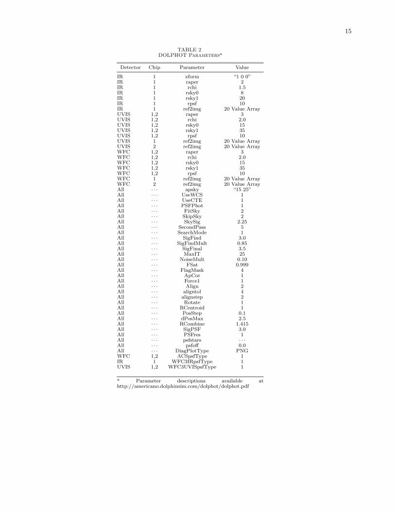
15

TABLE 2DOLPHOT Parametersa

Detector Chip Parameter Value

IR 1 xform “1 0 0”IR 1 raper 2IR 1 rchi 1.5IR 1 rsky0 8IR 1 rsky1 20IR 1 rpsf 10IR 1 ref2img 20 Value ArrayUVIS 1,2 raper 3UVIS 1,2 rchi 2.0UVIS 1,2 rsky0 15UVIS 1,2 rsky1 35UVIS 1,2 rpsf 10UVIS 1 ref2img 20 Value ArrayUVIS 2 ref2img 20 Value ArrayWFC 1,2 raper 3WFC 1,2 rchi 2.0WFC 1,2 rsky0 15WFC 1,2 rsky1 35WFC 1,2 rpsf 10WFC 1 ref2img 20 Value ArrayWFC 2 ref2img 20 Value ArrayAll · · · apsky “15 25”All · · · UseWCS 1All · · · UseCTE 1All · · · PSFPhot 1All · · · FitSky 2All · · · SkipSky 2All · · · SkySig 2.25All · · · SecondPass 5All · · · SearchMode 1All · · · SigFind 3.0All · · · SigFindMult 0.85All · · · SigFinal 3.5All · · · MaxIT 25All · · · NoiseMult 0.10All · · · FSat 0.999All · · · FlagMask 4All · · · ApCor 1All · · · Force1 1All · · · Align 2All · · · aligntol 4All · · · alignstep 2All · · · Rotate 1All · · · RCentroid 1All · · · PosStep 0.1All · · · dPosMax 2.5All · · · RCombine 1.415All · · · SigPSF 3.0All · · · PSFres 1All · · · psfstars · · ·All · · · psfoff 0.0All · · · DiagPlotType PNGWFC 1,2 ACSpsfType 1IR 1 WFC3IRpsfType 1UVIS 1,2 WFC3UVISpsfType 1

a Parameter descriptions available athttp://americano.dolphinsim.com/dolphot/dolphot.pdf

16

TABLE 3Crowding and square of sharpness

values used for measurement cullingand flagginga

Camera Sharpness Squared Crowding

UVIS 0.15 1.3ACS 0.2 2.25IR 0.15 2.25

a Maximum allowed values for the crowdingand the square of the sharpness value appliedto the combined measurement for each starin each band independently. Measurementswith lower values are given a GST value of1, and those with higher values are given aGST flag of 0. Measurements that did notpass the sharpness criterion in any band werecompletely rejected.

TABLE 4Number of stars with reliable measurements in each band in each brick

Brick Total F275W F336W F475W F814W F110W F160W

1 7739068 18310 268608 6587303 7276966 5605734 45477192 5389720 32745 150598 4064105 4635696 3753250 27409613 7420074 25280 126152 6296160 6969507 5327618 41616624 5699925 38868 165470 4430452 4966957 3949133 29471355 7017006 27125 121143 5871771 6513479 5070041 40006216 5737431 35452 154325 4413826 4969404 3928435 28984937 6548176 31481 110925 5307224 5917345 4654753 36962698 5619644 33584 151109 4256729 4817534 3841721 27870509 6107219 38838 144052 4589795 5361598 4255312 328284310 5286304 37461 114350 3826009 4445694 3666566 260479411 2944424 16185 41962 2257404 2560174 2007530 149097512 5037810 32830 130383 3715558 4286834 3433973 242121913 5701760 37060 100222 4178398 4886377 3907437 284429414 5381346 37474 139786 3945878 4583746 3649396 256538815 5506459 47311 201660 3579821 4638748 3876490 283130216 4978208 36893 135707 3453638 4152284 3371484 232459617 4928251 35865 144164 3299131 4072788 3462695 239827718 3988686 31269 87305 2588023 3199622 2691382 172425019 4030587 27500 76068 2638976 3259447 2740509 176275020 3116348 38093 70767 1843219 2390934 2064556 127388521 3207788 31108 90925 1897030 2535071 2228104 141452122 2718684 25772 55894 1495505 2002241 1739825 106391423 2756854 22383 53262 1613141 2134913 1780956 1114743

17

TA

BL

E5

Exam

ple

of

the

Photom

etry

Catalog

(full

catalog

avail

able

onlin

e)

RA

(J2000)

DE

C(J

2000)

F275W

S/N

GS

TF

336W

S/N

GS

TF

475W

S/N

GS

TF

814W

S/N

GS

TF

110W

S/N

GS

TF

160W

S/N

GS

T

10.5

80256333

41.2

441757179

26.6

81.0

F99.9

99

-0F

24.6

03

42.3

T21.8

5125.7

T20.9

81

117.5

T20.0

27

124.2

T10.5

802572159

41.2

457103763

23.8

48

8.2

T27.8

01

0.8

F25.3

92

19.4

T23.6

03

35.7

T22.5

38

33.2

T21.7

77

31.8

F10.5

8025753

41.2

45922544

99.9

99

-0.2

F99.9

99

-0.1

F25.5

73

20.7

T23.4

28

40.8

T22.8

14

28.7

T22.2

79

22.2

T10.5

802579935

41.2

460588596

99.9

99

-0.4

F26.7

06

2.2

F25.4

15

24.7

T23.3

29

45.6

T22.1

06

49.5

T21.3

29

48.7

T10.5

802580564

41.2

434928097

26.5

53

1.1

F99.9

99

-1.7

F99.9

99

-1.4

F21.8

61

123.8

T20.0

65

235.2

T18.9

69

300.9

T10.5

802582443

41.2

474459936

99.9

99

-1.3

F27.1

88

1.4

F24.9

31

34.0

T21.9

97

108.1

T21.0

97

112.3

T20.1

49

133.1

T10.5

802583084

41.2

479862568

99.9

99

-0.3

F26.5

28

2.5

F25.4

88

21.9

T22.8

363.8

T22.0

22

54.5

T21.2

64

51.9

T10.5

802586378

41.2

493851795

99.9

99

-0.3

F99.9

99

-1.2

F26.9

32

6.7

T24.4

317.2

T23.2

29

19.1

T23.0

48

10.3

F10.5

802594502

41.2

488740433

99.9

99

-1.6

F99.9

99

-1.6

F25.7

14

18.5

T23.2

45

48.7

T22.4

96

40.2

T21.3

67

46.5

T10.5

802601961

41.2

440702789

99.9

99

-0.5

F27.6

88

0.9

F26.7

22

7.4

T25.0

29

10.0

T99.9

99

-1.5

F99.9

99

-0.7

F10.5

80261801

41.2

473107079

99.9

99

-0.3

F27.5

34

1.0

F25.0

32

30.4

T22.7

41

59.8

T21.9

47

53.0

T21.2

01

49.9

T...

...

...

...

...

...

...

...

...

...

...

...

...

...

...

...

...

...

...

...

18

TABLE 6Standard deviation of magnitude offsets and median sharpness for different magnitude bins in different filters.

Mag F475W Offset F475W Sharp F814W Offset F814W Sharp F110W Offset F110W Sharp F160W Offset F160W Sharp

22.5 · · · · · · 0.016 0.010 0.013 0.006 0.014 0.00623.5 0.019 0.018 0.017 0.009 0.013 0.006 0.017 0.00624.5 0.022 0.017 0.018 0.007 0.023 0.006 0.049 0.00925.5 0.027 0.014 0.021 0.004 0.048 0.007 0.051 0.01626.5 0.031 0.010 0.044 0.003 0.041 0.012 · · · · · ·27.5 0.043 0.004 0.077 0.007 · · · · · · · · · · · ·28.5 0.113 0.012 · · · · · · · · · · · · · · · · · ·

19

TA

BL

E7

Exam

ple

of

the

Artif

icia

lStar

Catalog

(full

catalog

avail

able

onlin

e)

RA

(J2000)

DE

C(J

2000)

F275W

INF

275W

OUT

F336W

INF

336W

OUT

F475W

INF

475W

OUT

F814W

INF

814W

OUT

F110W

INF

110W

OUT

F160W

INF

160W

OUT

10.8

6064898

41.4

6919167

25.0

84

99.9

99

23.2

12

23.2

05

22.0

26

22.0

16

20.2

07

20.1

89

19.5

86

19.5

73

19.0

13

18.9

93

10.8

6064901

41.4

4335114

26.9

24

99.9

99

26.2

51

25.9

19

25.9

76

25.7

724.4

65

24.1

92

23.9

86

24.0

18

23.6

58

99.9

99

10.8

6065098

41.4

6782277

28.9

15

99.9

99

26.7

28

99.9

99

22.8

13

22.8

39

19.4

56

19.4

75

18.2

88

18.2

96

17.2

02

17.2

14

10.8

6065183

41.4

5522179

31.8

83

99.9

99

29.8

76

99.9

99

26.0

91

26.1

98

22.4

39

22.4

45

21.0

91

21.1

119.9

19.9

13

10.8

6065268

41.4

3842322

22.5

25

22.6

16

22.3

62

22.3

59

22.7

29

22.7

04

22.1

14

22.0

21

21.9

65

21.8

65

21.8

27

21.5

85

10.8

60653

41.4

3563822

28.7

65

99.9

99

26.2

53

99.9

99

22.4

81

22.4

27

19.3

03

19.3

08

18.1

69

18.1

75

17.0

86

17.0

99

10.8

6065355

41.4

4038206

31.3

63

99.9

99

31.3

11

99.9

99

26.6

55

26.6

03

22.0

13

22.0

06

20.3

06

20.3

06

18.9

73

18.9

88

10.8

6065372

41.4

3920687

26.7

31

99.9

99

26.1

85

99.9

99

25.6

09

25.8

02

24.8

89

25.1

48

24.6

25

99.9

99

24.4

57

99.9

99

10.8

6065452

41.4

3584972

28.8

91

99.9

99

26.2

18

99.9

99

24.6

49

24.7

03

22.6

34

22.6

49

21.9

29

22.0

29

21.1

52

21.1

45

10.8

6065506

41.4

4638759

30.3

42

99.9

99

28.5

82

99.9

99

24.5

38

24.6

28

20.8

86

20.8

91

19.5

91

19.5

84

18.4

45

18.4

54

10.8

6065509

41.4

5877434

30.2

93

99.9

99

27.2

07

99.9

99

25.1

524.7

77

22.6

83

22.4

59

21.7

921.7

13

20.8

92

20.8

35

...

...

...

...

...

...

...

...

...

...

...

...

...

...

20

TABLE 8RMS, Bias, and DOLPHOT-reported uncertainties from our

artificial star tests as a function of stellar density, filter,and magnitude. Full table available in electronic form only.

Density Filter Magnitude Bias RMS DOLPHOT Ratio

0.04 F275W 16.0 0.005 0.015 0.002 7.40.04 F275W 16.5 0.005 0.012 0.003 4.00.04 F275W 17.0 0.006 0.012 0.004 3.10.04 F275W 17.5 0.007 0.011 0.005 2.30.04 F275W 18.0 0.009 0.012 0.006 2.00.04 F275W 18.5 0.011 0.016 0.008 1.90.04 F275W 19.0 0.013 0.018 0.010 1.80.04 F275W 19.5 0.015 0.023 0.013 1.70.04 F275W 20.0 0.018 0.029 0.017 1.70.04 F275W 20.5 0.022 0.037 0.022 1.7... ... ... ... ... ... ...

a Density of stars with 18.5<F160W<19.5 per arcsec2.

TABLE 950% completeness limits for each band at a variety of stellar densities.

Brick Field Stellar Densitya F275Wlim F336Wlim F475Wlim F814Wlim F110Wlim F160Wlim

21 15 0.041 25.06 26.04 27.97 26.85 26.11 25.169 2 0.185 24.96 25.95 27.60 26.03 24.99 23.995 10 0.516 24.83 25.90 27.34 25.17 23.80 22.883 5 1.549 24.81 25.87 26.25 23.89 22.72 21.701 5 4.304 24.64 25.34 25.41 23.05 21.89 20.681 10 7.532 24.41 25.08 24.72 22.39 21.07 19.99

a Density of stars with 18.5<F160W<19.5 per arcsec2.

TABLE 10Fields with elevated

IR background

Brick Field Filter

2 7 F110W4 2 F110W4 13 F110W7 16 F110W7 17 F110W8 7 F110W8 9 F110W10 17 F110W13 7 F110W16 2 F160W16 15 F110W17 4 F110W17 18 F110W18 3 F110W18 7 F110W18 13 F110W18 14 F110W18 15 F110W21 6 F110W22 2 F160W22 3 F160W22 7 F160W22 8 F110W22 13 F160W22 14 F110W23 11 F110W23 13 F110W23 14 F110W23 14 F110W23 15 F110W23 15 F160W

21

B23

B22B21

B20B19

B18B17

B16B15

B14B13

B12B11

B10

B09

B08

B07

B06

B05

B04

B03

B02

B01

Fig. 1.— PHAT footprints. The pattern of the 23 “bricks” of the PHAT survey are shown on a GALEX NUV image oriented withnorth up and east left.

22

0 1000 2000 3000 4000 5000 6000

F12

F06F01 F02 F03 F04

F18

F05

F07 F08 F09 F10

F17

F11

F13 F14 F15 F16

Fig. 2.— IR exposure map with labeled field numbers for a generic PHAT brick. The grayscale is in units of seconds of exposuretime.

23

0 5000 10000 15000 20000 25000 30000

Fig. 3.— Total exposure map for a generic PHAT brick including all cameras. The grayscale is in units of seconds of exposure time.

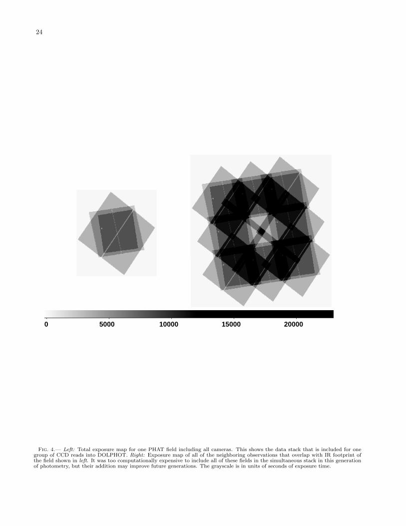
24

0 5000 10000 15000 20000

Fig. 4.— Left: Total exposure map for one PHAT field including all cameras. This shows the data stack that is included for onegroup of CCD reads into DOLPHOT. Right: Exposure map of all of the neighboring observations that overlap with IR footprint ofthe field shown in left. It was too computationally expensive to include all of these fields in the simultaneous stack in this generationof photometry, but their addition may improve future generations. The grayscale is in units of seconds of exposure time.

25

Fig. 5.— Stacked image quality in each camera. Left panels show the exposure map (1′′ per pixel; darker gray indicates moreexposure) of the 17′′×17′′ location shown on the right in UVIS (F336W; top) ACS (F475W; middle), and IR (F160W; bottom). Theimages (grayscale inverted) show an area of complex overlaps including the 180◦ flip at the middle of Brick 14. The precision alignmentresults in virtually seamless images.

26

Fig. 6.— Alignment quality of all images in the survey. Upper Left: One-sigma uncertainty ellipses for alignment between pairsof CCD reads for all F475W data in Brick 15. The ellipses are fit via expectation-maximization of a foreground-background modelof all star-to-star matches between the pair of exposures. Each red ellipse shows the uncertainty between one pair of F475W CCDreads. Each blue ellipse shows the uncertainty between an F475W CCD read and a F814W CCD read. Each gray ellipse shows theuncertainty between an F475W CCD read and the ground-based absolute astrometric reference.Upper Right: Same as upper left, butfor F160W CCD read, and gray circles show alignment to the F475W images, red to other F160W reads, and blue to F110W reads.Lower Left: Same as upper right, but for F336W, and gray circles show alignment to the F475W images, red to other F336W reads,and blue to F275W reads. Lower Right: The scatter of alignment stars is computed as the standard deviation of the distributionof alignment stars in units of native pixels of the CCD read being aligned. Blue indicates short (<20 seconds) exposure times. Redindicates UVIS images of the North and East edges of the survey footprint.

27

Fig. 7.— Example of raw phot.fits output in the optical (left) and measurements culled from the raw DOLPHOT output (phot.fits)when producing the ST tables (st.fits) because no single band had a measurement with signal-to-noise>4 and a sharpness value thatpassed our cut from Table 3 (left). No CMD feature is seen in the culled measurements, showing the low quality of these measurements.

Fig. 8.— UV, optical, and IR CMDs of a small random sample from the catalog, color-coded to show the number of bands withgood measurements. In all panels, black, blue, cyan, orange, and red points show stars with good measurements in 2, 3, 4, 5, and6 bands, respectively. Left: UV CMD produced from all measurements where both bands passed our GST criteria. Center: OpticalCMD produced from all measurements where both bands passed our GST criteria. Right: IR CMD produced from all measurementswhere both bands passed our GST criteria.

28

Fig. 9.— UV color magnitude diagram for all F275W and F336W measurements in the survey. Numbers in the upper-right of thepanels refer to relative stellar densities shown on the map in Figure 10. In this case, the full survey, covering all stellar densities, isshown. Left: Fraction of measurements flagged as not passing our quality cuts in either of the two bands. Right: CMD producedshowing only measurements that pass our quality cuts in both bands.

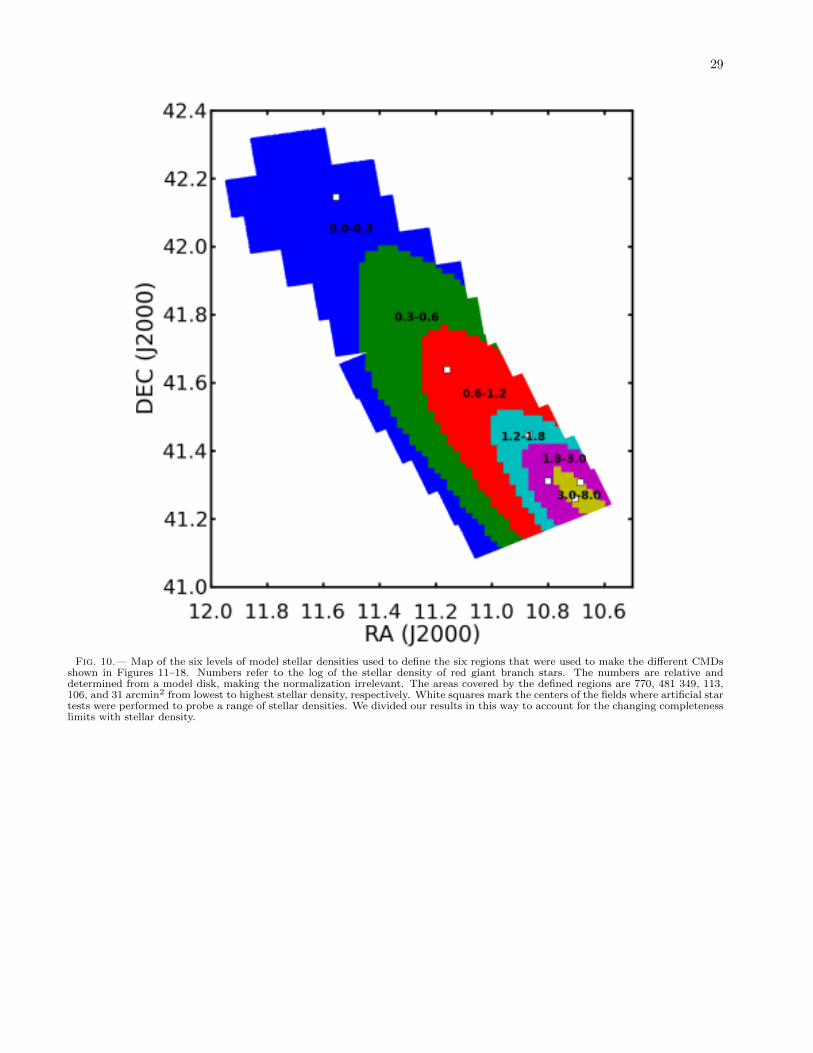
29

Fig. 10.— Map of the six levels of model stellar densities used to define the six regions that were used to make the different CMDsshown in Figures 11–18. Numbers refer to the log of the stellar density of red giant branch stars. The numbers are relative anddetermined from a model disk, making the normalization irrelevant. The areas covered by the defined regions are 770, 481 349, 113,106, and 31 arcmin2 from lowest to highest stellar density, respectively. White squares mark the centers of the fields where artificial startests were performed to probe a range of stellar densities. We divided our results in this way to account for the changing completenesslimits with stellar density.

30

Fig. 11.— Fraction of F336W or F475W measurements flagged as not passing our quality cuts as a function of color and magnitude.

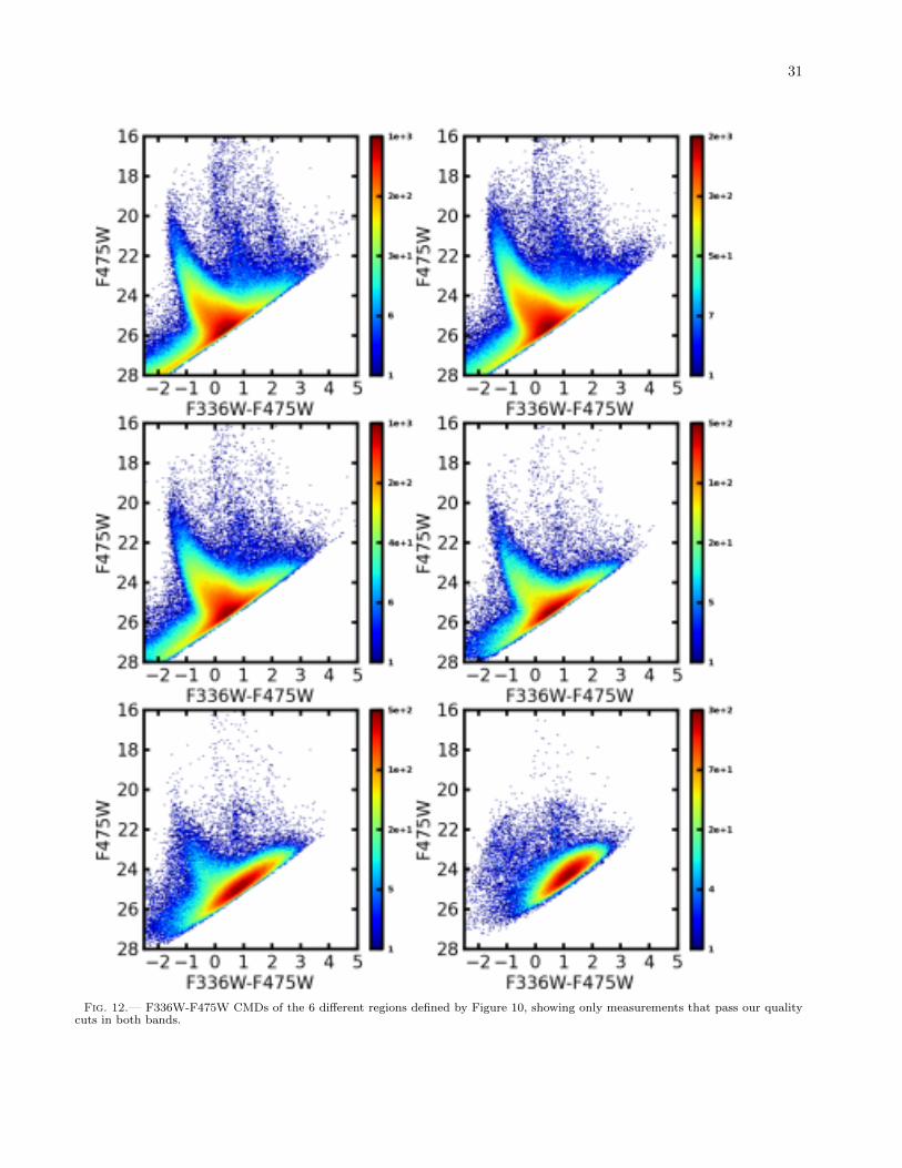
31

Fig. 12.— F336W-F475W CMDs of the 6 different regions defined by Figure 10, showing only measurements that pass our qualitycuts in both bands.

32

Fig. 13.— F475W-F814W at different stellar densities of the fraction of stars passing our cuts, as in Figure 11.

33

Fig. 14.— F475W-F814W CMDs at different stellar densities after quality cuts, as in Figure 12.

34

Fig. 15.— F475W-F160W CMDs at different stellar densities of the fraction of stars passing our cuts, as in Figure 11.

35

Fig. 16.— F475W-F160W CMDs at different stellar densities after quality cuts, as in Figure 12.

36

Fig. 17.— F110W-F160W CMDs at different stellar densities of the fraction of stars passing our cuts, as in Figure 11.

37

Fig. 18.— F110W-F160W CMDs at different stellar densities after quality cuts, as in Figure 12.

38

Fig. 19.— Model predictions for the CMDs of the total foreground population of the 0.5 deg2 PHAT survey. The foreground starsdraw nearly-vertical sequences at colors 1<F275W-F336W<3, 0<F336W-F475W<2, 1<F475W-F814W<4, 1.5<F475W-F160W<5,and 0.4<F110W-F160W<0.8. Although the foreground stars make up <0.02% of the catalog, these sequences are still evident in theobserved CMDs show in Figures 9-18.

39

Fig. 20.— Root mean square scatter in the positive and negative directions (thick) and median (thin) of artificial star tests as afunction of (and relative to) input magnitude in all 6 bands at 5 different stellar densities (number of stars with 18.5<F160W<19.5per arcsec2). Both the bias and the RMS scatter are very small at the bright end. In the UV bands, the errors at the faint end onlyreach ∼0.2 mag, and the bias is faintward. In redder bands with low crowding, the bias is near 0, and the errors are ∼0.2 mag at thefaint end. In crowded regions, the bias and the errors can reach >0.5 mag, and the bias is brightward.

40

Fig. 21.— Root mean square scatter in the positive and negative directions (thick) and median (thin) in color as a function ofmagnitude and stellar density (number of stars with 18.5<F160W<19.5 per arcsec2). Color scatter increases substantially with stellardensity, but the bias remains low, except right at the magnitude limit, where the bias can be large and relatively unpredictable.

41

Fig. 22.— Ratio of the RMS from artificial star tests to the DOLPHOT-reported uncertainty as a function of magnitude for a rangeof stellar densities. Each panel gives the results for a different filter, as labeled, and each line color represents a different stellar density(number of stars with 18.5<F160W<19.5 per arcsec2), as labeled.

42

Fig. 23.— Completeness as a function of stellar density (number of stars with 18.5<F160W<19.5 per arcsec2) in the survey. Thereis a clear trend that the red bands are crowding-limited over much of the survey, while the UV bands are not.

43

010

0020

0030

0040

00A

CS

refe

renc

epi

xels

:x

0

1000

2000

3000

4000

ACSreferencepixels:y

F47

5W

−0.

08

−0.

06

−0.

04

−0.

02

0.00

0.02

0.04

0.06

0.08

010

0020

0030

0040

00A

CS

refe

renc

epi

xels

:x

0

1000

2000

3000

4000

ACSreferencepixels:y

F81

4W

−0.

08

−0.

06

−0.

04

−0.

02

0.00

0.02

0.04

0.06

0.08

010

0020

0030

0040

00A

CS

refe

renc

epi

xels

:x

0

1000

2000

3000

4000

ACSreferencepixels:y

F47

5W-

F81

4W

−0.

05

−0.

04

−0.

03

−0.

02

−0.

01

0.00

0.01

0.02

0.03

0.04

0.05

050

010

0015

0020

0025

0030

0035

0040

00R

efer

ence

imag

epi

xels

:x

0

500

1000

1500

2000

2500

3000

3500

4000

Referenceimagepixels:y

F11

0W

−0.

040

−0.

032

−0.

024

−0.

016

−0.

008

0.00

0

0.00

8

0.01

6

0.02

4

0.03

2

0.04

0

050

010

0015

0020

0025

0030

0035

0040

00R

efer

ence

imag

epi

xels

:x

0

500

1000

1500

2000

2500

3000

3500

4000

Referenceimagepixels:yF

160W

−0.

040

−0.

032

−0.

024

−0.

016

−0.

008

0.00

0

0.00

8

0.01

6

0.02

4

0.03

2

0.04

0

050

010

0015

0020

0025

0030

0035

0040

00R

efer

ence

imag

epi

xels

:x

0

500

1000

1500

2000

2500

3000

3500

4000

Referenceimagepixels:y

F11

0W-

F16

0W

−0.

040

−0.

032

−0.

024

−0.

016

−0.

008

0.00

0

0.00

8

0.01

6

0.02

4

0.03

2

0.04

0

Fig

.24.—

Syst

emati

cm

agn

itu

de

an

dco

lor

vari

ati

on

sfo

rth

esa

me

stars

mea

sure

don

diff

eren

tp

art

sof

the

AC

S/W

FC

cam

era

inF

475W

(top

left

),F

814W

(top

middle

),an

dF

475W

-F814W

(toprigh

t)fr

om

ou

tsid

eof

the

bu

lge,

an

don

diff

eren

tp

art

sof

WF

C3/IR

inF

110W

(bottom

left

),F

160W

(bottom

middle

),an

dF

110W

-F160W

(bottom

righ

t)fr

om

the

over

lap

bet

wee

nb

rick

s9

an

d11.

Th

esy

stem

ati

cer

rors

as

afu

nct

ion

of

bri

ghtn

ess

are

∼±

0.0

2-0

.05

(see

Tab

le6).

44

Fig. 25.— Median sharpness values for the all stars outside of the bulge as a function of position on the ACS/WFC camera inF475W (top left) and F814W (top right), and as a function of postion on the WFC3/IR camera in F110W (bottom left) and F160W(bottom right). The systematic patterns are the same as those seen in magnitude, suggesting the PSF library as the dominant sourceof systematic errors.

45

Fig. 26.— Median F475W sharpness values vs. F475W magnitude offset at each location on the ACS detector in several magnitudebins. Upper-left: The relation at F475W=24.5, showing a strong anti-correlation. Upper-right: The relation at F475W=25.5, showingthe correlation begin to steepen as the range of median sharpness drops with increasing magnitude. Lower-left: The relation atF475W=26.5, showing a continued steepening as the sharpness range continues to drop. Lower-right: The relation at F475W=27.5,where the sharpness measurements no longer have the necessary precision to detect the correlation.

46

0 500 1000 1500 2000 2500 3000 3500 40000

500

1000

1500

2000

2500

3000

3500

4000

25 < F475W < 26

−0.08

−0.06

−0.04

−0.02

0.00

0.02

0.04

0.06

0.08

0 500 1000 1500 2000 2500 3000 3500 40000

500

1000

1500

2000

2500

3000

3500

4000

28 < F475W < 29

−0.08

−0.06

−0.04

−0.02

0.00

0.02

0.04

0.06

0.08

0 500 1000 1500 2000 2500 3000 3500 40000

500

1000

1500

2000

2500

3000

3500

4000

24 < F814W < 25

−0.08

−0.06

−0.04

−0.02

0.00

0.02

0.04

0.06

0.08

0 500 1000 1500 2000 2500 3000 3500 40000

500

1000

1500

2000

2500

3000

3500

4000

27 < F814W < 28

−0.08

−0.06

−0.04

−0.02

0.00

0.02

0.04

0.06

0.08

Fig. 27.— Systematic magnitude variations for the same stars measured on different parts of the ACS/WFC camera in F475W(top row) and F814W (bottom row). The pattern at the for brighter stars (left side) shows a grid pattern and correlation withsharpness indicative of PSF model origin, while the pattern for faint stars (right side) is symmetric about the chip gap, indicative ofa CTE-correction origin.

47

Fig. 28.— The F814W magnitude (left) and cumulative magnitude (right) distributions around the tip of the red giant branch for34 6′ × 6′ regions of the survey. Note the tight consistency across the entire PHAT survey.

Fig. 29.— The F160W magnitude (left) and cumulative magnitude (right) distributions around the tip of the red giant branch for40 6′ × 6′ regions of the survey. Note the tight consistency across the entire PHAT survey.

48

Fig. 30.— Histogram of the F814W magnitude of the center of the red clump feature for 298 3′ × 3′ regions of the survey. They areall consistent with one another to ±0.05 mag, and the distribution is quite symmetric, suggesting that any biases in our photometryare below this level of precision at this magnitude.

−0.5 0.0 0.5 1.0 1.5 2.0 2.5

F110W−F160W

22

20

18

16

F1

60

W

44450 stars90% with F160W < 19.34

−0.5 0.0 0.5 1.0 1.5 2.0 2.5

F110W−F160W

22

20

18

16

F1

60

W

107645 stars90% with F160W < 20.46

−0.5 0.0 0.5 1.0 1.5 2.0 2.5

F110W−F160W

22

20

18

16

F1

60

W

277720 stars90% with F160W < 21.11

Fig. 31.— Left: CMD from IR photometry of Brick 1, Field 5 when only the IR data are included in the DOLPHOT process. MiddleSame as right with updated DOLPHOT parameters. Right CMD from IR photometry with updated DOLPHOT parameters when allUV, optical, and IR data centered on the Brick 1, Field 5 are included in the DOLPHOT process. All panels provide the total numberof stars and the magnitude which 90% of the stars are brighter than.

49

Fig. 32.— Left: Fraction of raw optical detection lost as a function of color and magnitude. Contour levels show the locations ofCMD features in the full sample of the field. Very few (<10%) are lost inside of CMD features. Right: Same as left, but for culledoptical detections. The fractions is very low <5% inside of CMD features.

11.4011.4511.5011.5511.6011.6511.70RA (deg)

42.10

42.15

42.20

42.25

Dec

(deg

)

0.0

1.5

3.0

4.5

6.0

7.5

9.0

10.8510.9010.9511.0011.0511.10RA (deg)

41.10

41.15

41.20

41.25

Dec

(deg

)

0.0

2.5

5.0

7.5

10.0

12.5

15.0

17.5

20.0

22.5

Fig. 33.— Left: Stellar density map in Brick 17, where crowding is less severe. Right: Same as Left, but for Brick 2, where crowdingis more severe. Grayscale units are in stars per arcsec2. The chip gap features become much more apparent as crowding increases.

10.9010.9511.0011.0511.1011.15RA (deg)

41.20

41.25

41.30

41.35

Dec

(deg

)

Per-camera F110W in [20, 21]

0

4

8

12

16

20

24

28

32

10.9010.9511.0011.0511.1011.15RA (deg)

41.20

41.25

41.30

41.35

Dec

(deg

)

Six-filter F110W in [20, 21]

0

4

8

12

16

20

24

28

32

Fig. 34.— Stellar density maps of Brick 02 showing bright stars (20<m<21) with good measurements in F110W. Left: Map producedusing results from single-camera photometry. Right: Map produced using results from multi-camera photometry. Grayscale units arestars per 5′′×5′′ bin.

50

10.9010.9511.0011.0511.1011.15RA (deg)

41.20

41.25

41.30

41.35

Dec

(deg

)

Per-camera F110W in [24, 25]

0

40

80

120

160

200

240

280

10.9010.9511.0011.0511.1011.15RA (deg)

41.20

41.25

41.30

41.35

Dec

(deg

)

Six-filter F110W in [24, 25]

0

40

80

120

160

200

240

280

Fig. 35.— Stellar density maps of Brick 02 showing faint stars (24<m<25) with good measurements in F110W. Left: Map producedusing results from single-camera photometry. Right: Map produced using results from multi-camera photometry. Grayscale units arestars per 5′′×5′′ bin.