Balance Winds

• Geostrophic Balance• Gradient Wind• Cyclostrophic Wind Balance• Balance with Friction / Ekman Balance

Geostrophic BalanceThe equation of motion can be written as:

)k-gG( vector nalgravitatio theis G

friction of effects therepresents F

termCoriolis thecalled is V2

earth theof raterotation the toingcorrespond day/2

pole)north thefrom upward pointing (positiveearth theoflocity angular ve theis where

GFV2p1dtVd

rrr

r

rr

r

rrrrr

=

×Ω

π=Ω

Ω

+−×Ω−∇ρ

−=

Coriolis Term

[ ]

φΩ=φΩ=

+−−=×Ω−∴

φΩ+φΩ+φΩφΩ=

φΩφΩ−=×Ω−

ins2f and osc2f where

kufjfui)wffv(V2

ku)osc(-ju)ins(iv)sin-wosc(2-

wvusincos0kji

2V2

rrrrr

rrr

rr

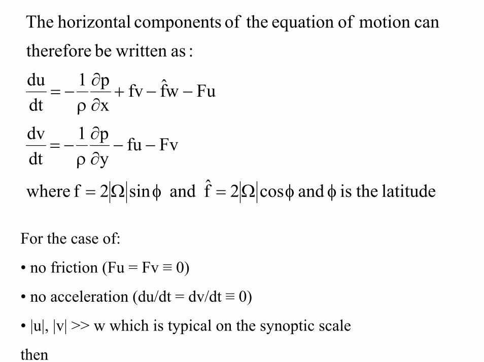
latitude theis and cos2f and sin2f where

Fvfuyp1

dtdv

Fuwffvxp1

dtdu

:as written be thereforecan motion ofequation theof components horizontal The

φφΩ=φΩ=

−−∂∂

ρ−=

−−+∂∂

ρ−=

For the case of:

• no friction (Fu = Fv ≡ 0)

• no acceleration (du/dt = dv/dt ≡ 0)

• |u|, |v| >> w which is typical on the synoptic scale

then

vxp

f1 v fv

xp10

uyp

f1-u fu

yp10

g

g

≡∂∂

ρ=⇒+

∂∂

ρ−=

≡∂∂

ρ=⇒−

∂∂

ρ−=

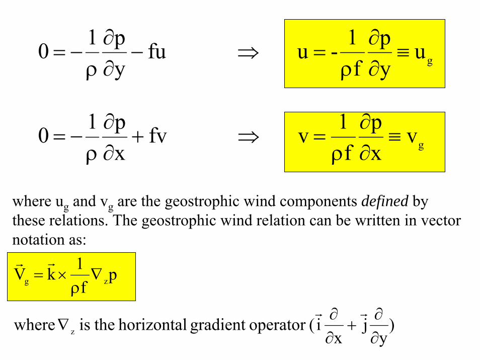
where ug and vg are the geostrophic wind components defined by these relations. The geostrophic wind relation can be written in vector notation as:

)y

jx

i(operator gradient horizontal theis where

pf

1kV

z

zg

∂∂

+∂∂

∇

∇ρ

×=

rr

rr

0yp

f1

xp

f1

100kji

jviuV

:product crossvector theof definition theusing checked becan This

pf

1kV

ggg

zg

∂∂

ρ∂∂

ρ

=+=

∇ρ

×=

rrr

rr

pf

1kV zg ∇ρ

×=rr

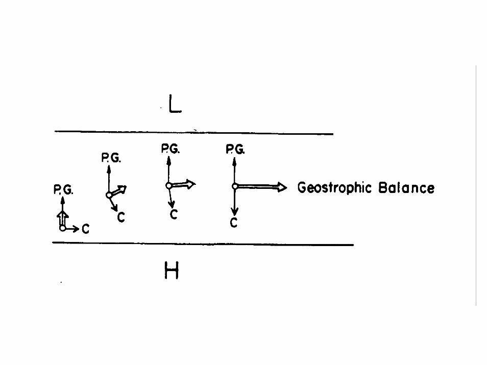
windcgeostrophi for thestraight is flow that theassumed isIt latitudes lowat achievedrarely is balance cGeostrophi

latitudes lowat 0 f because latitudeslower at Vstronger in result willp of egiven valuA

)Vlarger theplarger (thegradient pressure the toalproportionlinearlyalmost is V height,given aat constant nearly is As

hemispheresouthern in theleft the toand hemispherenorthern in theright the tois pressurehigh thesuch that directed is V

isobars) the toparallel isdirection wind (the p lar toperpendicu and horizontal bemust V

force Coriolis theand forcegradient pressureebetween thbalancetheis windcgeostrophi The

gz

gz

g

g

zg

•

•

→∇•

∇ρ•

•

∇•

•

r

rr

r

r

xp

f1v

yp

f1-u

g

g

∂∂

ρ=

∂∂

ρ=

Gradient Wind• The geostrophic wind balance assumes that the wind

flow is straight• A more general form of a balanced wind can be

obtained if accelerations due to curvature in the height or pressure fields are taken into account (remember that changes in the direction of the velocity vector with time result in acceleration)

• The gradient wind like the geostrophic wind is frictionless, but it is not unaccelerated

force lcentrifuga simply the isequation above theof side handright The

r of magnitude theis R ectorposition v theis r

indgradient wfor standsgr subscript thewhere

)(dtVd

:curvature todueon accelerati for the for the expressionan obtain can wenotes sPielke' Following

wind.cgeostrophi for the it was as zeronot is dtVd termthe

curvature, of effects the todueon accelerati have now weAs

21dtVd

:aswritten becan motion ofequation The

T

2

r

r

rrr

r

rrrrr

rR

V

GFVp

T

gr−=

+−×Ω−∇−=ρ

The direction of the unit vector at points A, B, C and D are denoted by the appropriate Cartesian unit vector

)r(R

vuj

dtdvi

dtdu )r(

RV

dtVd

T

2gr

2gr

T

2

gr rrrrrr

−+

=+⇒−=

rr−

T

2gr

Ru

dtdv

0dtdu

−=

=

T

2gr

Rv

dtdu

0dtdv

−=

=

T

2gr

Ru

dtdv

0dtdu

=

=

T

2gr

Rv

dtdu

0dtdv

=

=

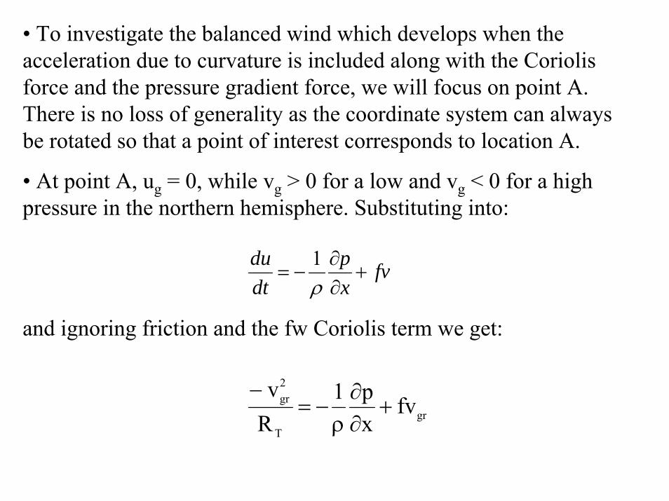
• To investigate the balanced wind which develops when the acceleration due to curvature is included along with the Coriolis force and the pressure gradient force, we will focus on point A.There is no loss of generality as the coordinate system can always be rotated so that a point of interest corresponds to location A.

• At point A, ug = 0, while vg > 0 for a low and vg < 0 for a high pressure in the northern hemisphere. Substituting into:

and ignoring friction and the fw Coriolis term we get:

fvxp

dtdu

+∂∂

−=ρ1

grT

2gr fv

xp1

Rv

+∂∂

ρ−=

−

)(

:get we1- as

1

2

2

ggrgrgT

gr

g

grT

gr

vvffvfvRv

fvxpNow

fvxp

Rv

−=+−=−

−=∂∂

+∂∂

−=−

ρ

ρ

• The velocity vgr which solves this relation is called the GRADIENT WIND

grgT

gr fvfvRv

+−=− 2

• The gradient wind balance is a three-way balance between the Coriolis force, the centrifugal force and the horizontal pressure gradient force

Centrifugal forcePressure gradient force

Coriolis force

2/)4(

:for v solve toformulaequation quadratic theUsing

0v:equation thisgRearrangin

)(

22

gr

2gr

2

gTTTgr

gTgrT

ggrgrgT

gr

fvRRffRv

fvRvfR

vvffvfvRv

+±−=

=−+

−=+−=−

• For a cyclone in the northern hemisphere, vg > 0 at A so that the radical is always real => no limit to the magnitude of the gradient wind

• For an anticyclone in the northern hemisphere, vg < 0 at A so that f2RT

2 > 4RTfvg => vg < fRT/4 for the radical to be real => there is a constraint on the magnitude of the pressure gradient force in anticyclones that does not exist for low pressures. This is the reason that lows on synoptic weather maps often have tight gradients while highs don’t.

ggrT

2gr

gTgrT2gr

vvfR

v

:asrewritten becan 0fvRvfRv

=+

=−+

• vgr < vg for a cyclone as vg > 0 at A

•|vgr| > |vg| for an anticyclone as vg < 0 at A

• These inequalities show that for the same pressure gradient (as represented by the geostrophic wind), the gradient balanced wind is stronger around a high than a low

• The gradient winds associated with a cyclone are SUBGEOSTROPHICbecause the centrifugal force helps to balance the acceleration due to the pressure gradient force, therefore the Coriolis terms fvgr and vgr don’t need to be as large

•The winds associated with an anticyclone are SUPERGEOSTROPHICbecause a large Coriolis acceleration (and hence large value of vgr) is needed to balance the sum of the acceleration due to the pressure gradient force and the centrifugal force

CFA > CFB > CFC

VgrA > VgrB > VgrC

Supergeostrophic

Subgeostrophic

GeostrophicA

B

C

Cyclostrophic Wind Balance

• When Coriolis force is neglected in the gradient wind balance we obtain a balance between the centrifugal force and the pressure gradient force – this balance is called the cyclostrophic wind balance

• Used to estimate wind speeds in small-scale vortices such as tornadoes and dust devils

1-

3-1-

d

2

2

s m 63 of windhiccyclostrop a have wouldm kg 1.25 ofdensity air an and km mb 100

ofgradient pressure a km, 0.5 of radius a with A tornado

v

:from obtained becan windhiccyclostrop The

1:balance windhiccyclostropFor

indgradient w for the 1 had We

xpR

xp

Rv

fvxp

Rv

T

T

d

grT

gr

∂∂

±=

∂∂

−=−

+∂∂

−=−

ρ

ρ

ρ

Balance with Friction• To evaluate the impact of friction on the resultant wind

balance, we can retain the friction terms in our horizontal equations of motion

stability amic thermodyn theand ground theaboveheight offunction a ist which coefficien drag a is C included.been havefriction of effects

that theindicates Fsubscript theand indgradient w the toangle someat generalin is V where

RV

:balance indgradient w theof form general more aobtain we

F and FSetting

D

F

2

T

2F

2v

2u

FDgF

DD

VCfVfV

vCuC

+=+

==

• Friction decelerates the flow and this turns the wind towards low pressure => results in low-level divergence out of anticyclones and low-level convergence into cyclones

• The frictional acceleration acts directly opposite to the direction of the wind

• The Coriolis acceleration is perpendicular to the wind direction

• The centrifugal force is also perpendicular to the instantaneous wind direction

Geostrophic wind Gradient wind

Frictional Effects

Summary of Balance WindsBalance Wind Assumptions BalanceGeostrophic flow

Neglect friction and acceleration due to curvature

Pressure gradient force and Coriolis force

Gradient wind Neglect friction Pressure gradient force, Coriolis force and centrifugal force

Cyclostrophic flow

Neglect friction and Coriolis force

Pressure gradient force and centrifugal force

Balance with Friction

All forces now included

Pressure gradient force, Coriolis force, centrifugal force and friction

pf

1kV zg ∇ρ

×=rr

grgT

gr fvfvRv

+−=− 2

xp

Rv

T

d

∂∂

−=−

ρ12

2

T

2F

RV

FDgF VCfVfV +=+

Continuity Equation• The equation of continuity

is given by:

• Physical interpretation: if a volume having dimensions ∆x, ∆ y and ∆ z experiences convergence, then the material volume decreases. However, since the amount of mass in a material volume remains constant, the density must increase

vDtD1 rr

⋅∇−=ρ

ρ

Source: Bluestein, 1992

• The continuity equation can also be expressed as:

This is the flux form of the continuity equation – says that mass in a volume can change locally only through flux convergence or divergence

• If we assume that the atmosphere is incompressible then the density of the parcel does not change:

vt

rρ⋅−∇=

∂ρ∂

0v

0vDtD

0DtD

=⋅∇=>

=⋅∇−=ρ

=>

=ρ

rr

rr

0v =⋅∇rr

• This means that for an incompressible atmosphere the atmosphere is three-dimensionally nondivergent

• The incompressible assumption implies that convergence in one or two directions must be balanced by divergence in the other direction(s) and that mass is conserved.

• The incompressible assumption is useful in helping to understand atmospheric systems that are not strongly dependant on compressibility. This approximation fails in strong thunderstorm updrafts, tornadoes etc

• For deep convection where the impacts of compressibility are important in the vertical, the following continuity equation is used:

where the base-state density ρ(z) is a function of height only

( )[ ] 0vz =ρ⋅∇rr

• Assume that the atmosphere behaves as an incompressible fluid:

Horizontal convergence => Vertical stretching

Horizontal divergence => Vertical shrinking

zw

yv

xu

:as written becan which

0zw

yv

xu

:ibleincompress is atmosphere that theassume weIf

z)w(

y)v(

x)u(

t

vt

:as formflux in written becouldequation continuityat theearlier th showed We

Divergence Horizontal

∂∂

−=∂∂

+∂∂

=∂∂

+∂∂

+∂∂

⎟⎟⎠

⎞⎜⎜⎝

⎛∂ρ∂

+∂ρ∂

+∂ρ∂

−=∂ρ∂

=>

ρ⋅−∇=∂ρ∂

43421

r

Level of Nondivergence• Vertical velocity is constrained to be zero at the ground and at the

tropopause• If w is nonzero, its sign is often the same at all levels in a column of the

troposphere => the sign of ∂w/∂z must reverse at some level. At this level:

which from the continuity equation implies

• This level is therefore called the level of nondivergence. It is typically found near 550-600mb.

• Rising motion above a level surface must be accompanied by convergence below and compensating divergence aloft.

• Similarly sinking motion must be accompanied by divergence below and convergence aloft

0zw=

∂∂

0Vdivyv

xu

HH ==∂∂

+∂∂ r

0Vdiv

0zw

HH <

>∂∂

r

0Vdiv

0zw

HH >

<∂∂

r

0Vdiv

0zw

HH >

<∂∂

r

0Vdiv

0zw

HH <

>∂∂

r

0Vdiv

0zw

HH =

=∂∂

r0Vdiv

0zw

HH =

=∂∂

rLevel of Nondivergence

Rising MotionSinking Motion

Convergence

DivergenceConvergence

Divergence

Pressure Tendency Equation

divergence horizontal theis div and vector windhorizontal theis V where

)()()()()(t

:atearlier th saw But we

tp

:is zat tendency pressure The

dp-

:it abovecolumn air theof weight by thegiven is (z)height any at pressure The

HH

0

0

p

r

r

zwVdiv

zw

yv

xu

dzt

gdzgt

pdpdzg

HH

zz

z

p

∂∂

−−=∂

∂−

∂∂

−∂

∂−=

∂∂

∂∂

=⎥⎦

⎤⎢⎣

⎡

∂∂

=∂∂

===

∫∫

∫ ∫∫

∞∞

∞

ρρρρρρ

ρρ

ρ

( )

dz)V(divgtp

0w :surface At the

wgdz)V(divgtp

wwdz)w(z

gFor

dz)w(z

gdz)V(divgtp

0zHH

0z

0z

zz

HHz

zz

zzHH

z

∫

∫

∫

∫∫

∞

==

=

∞

∞

∞

∞∞

ρ−=∂∂

=>

=ρ

ρ+ρ−=∂∂

∴

ρ−ρ=ρ∂∂

ρ∂∂

−ρ−=∂∂

r

r

r

0

Divergence and Vertical Motion

V. divergence average the toequal is interval theof middle

in the V. of value the,V. aryinglinearly vor V.constant of case

In the selected. is divergence average rticalcorrect ve theproviding)pp(V.-

: tointegrates side handright on the integral Thep/an smaller thmuch

typicallyare sderivative partialother thesince p)dp/(d:is side handleft theion toapproximat goodA

dpV.dpp

:p and p levels pressurebetween gIntegratin

divergence horizontal torefers divergence theand DtDp where V.

p

:as written becan equation continuity theatmosphere ibleincompressan assuming and scoordinate pressure Using

12

p

p

p

p

21

2

1

2

1

rr

rrrrrr

rr

rr

rr

∇

∇∇∇

−∇

∂ω∂

∂ω∂≈ω

∇−=∂ω∂

=ω∇−=∂ω∂

∫ ∫

motion sinking 0)0.( 850mbat divergence

motion rising0)0.( 850mbat econvergenc Therefore

300pp ere wh.

:following get the wesassumption e With thesneglected. thusis and 700mbat than thatlessmuch is

mb 1000at motion vertical that theis assumption picalAnother ty

mb. 700 and 1000between layer in the divergence average theto equal assumed becan mb 850at divergence thepurposesour For

mb 1000p and mb 700p and

then700mb and 1000between layer heconsider t :Example

pat and pat occurs where)(.

:have now weSo

700850

700850

21850700

110001

27002

221 11212

⇒>⇒>∇

⇒<⇒<∇

=−=∆∆∇=

====

−∇−=−

ω

ω

ω

ωωωω

ωωωω

V

V

mbppV

ppV

rr

rr

rr

rr

• Winds around high pressure systems diverge. Conservation of air mass requires subsidence over the high to replace the horizontally diverging air

• Similarly horizontally converging air around low pressure systems are associated with upward motion

Source: Stull, 2000

Baroclinity (Baroclinicity) and Barotropy

• Baroclinity (or Baroclinicity): The state of stratification in a fluid in which surfaces of constant pressure (isobaric) intersect surfaces of constant density (isoteric)

• Barotropy: The state of a fluid in which surfaces of constant density (or temperature) are coincident with surfaces of constant pressure; it is the state of zero baroclinity

• When there are temperature variations on an isobaric surface the atmosphere is said to be baroclinic. If there are no temperature variations the atmosphere is said to be barotropic

Barotropic Atmosphere Baroclinic Atmosphere

ρ and p surfaces coincide ρ and p surfaces intersect

p and T surfaces coincide p and T surfaces intersect

p and θ surfaces coincide p and θ surfaces intersect

No geostrophic wind shear

Geostrophic wind shear

No large-scale w Large-scale w

Examples of baroclinic systems:

• Cold fronts

• Sea breezes

• Mountain slope flows

Barotropic Baroclinic Barotropic

Barotropic Atmosphere

• eg: sea-breeze during early morning

• Pressure and density isolines are parallel / coincident

• No circulation

Baroclinic Atmosphere

• eg: sea-breeze in the afternoon

• Air over the land heats up more rapidly than that over water

• Pressure and density isolines intersect

• Circulation develops

• The lighter fluid over land “feels” the same pressure gradient force as that over the ocean – the lighter fluid will tend to rise more rapidly resulting in a net counterclockwise circulation

P1>P2>...>P5 and ρ1>ρ2>....>ρ5

Sea Land

Sea Land

High density Low density

Vorticity

• Vorticity: A vector measure of the rotation in a fluid, and is defined mathematically as the curl of the velocity:

• The vorticity of a solid rotation is twice the angular velocity vector

• In meteorology, vorticity usually refers to the vertical component of the vorticity

Vrr

×∇=ω

Components of Vorticity

k j i

kyu

xvj

xw

zui

zv

yw

wvuzyx

kji

V

rrr

rrr

rrr

rrr

ζ+η+ξ=⎟⎟⎠

⎞⎜⎜⎝

⎛∂∂

−∂∂

+⎟⎠⎞

⎜⎝⎛

∂∂

−∂∂

+⎟⎟⎠

⎞⎜⎜⎝

⎛∂∂

−∂∂

=

∂∂

∂∂

∂∂

=×∇=ω

• The components of the vorticity ξ (xi), η (eta) and ζ (zeta) are measures of the spin about the x, y and z axes.

Relative and Absolute Vorticity• Relative vorticity (or local vorticity) (ω):

– the vorticity as measured in a system of coordinates fixed on the earth's surface

– curl of the relative velocity

• Absolute vorticity (ωa)– the vorticity of a fluid particle determined with respect to

an absolute coordinate system (takes into account the rotation of the earth)

– curl of the absolute velocity

Vrrr

×∇=ω

aa Vrrr

×∇=ω

• The vertical component of the absolute vorticity vector (as defined above) is given by the sum of the vertical component of the vorticity with respect to the earth (the relative vorticity) and the vorticity due to the rotation of the earth (equal to the Coriolis parameter) f:

• The difference between absolute and relative vorticity is therefore simply the planetary vorticity (f=2Ω sin φ):

fa += ζζ

fyu

xv

yu

xv

a +∂∂

−∂∂

=∂∂

−∂∂

= ζζ

• Regions of large positive (negative) ζ tend to develop in association with cyclonic storms in the Northern (Southern) hemisphere – the distribution of relative vorticity is therefore an excellent diagnostic tool for weather analysis

• Absolute vorticity tends to be conserved following the motion at midtroposphericlevels – forms the basis to simple dynamical forecast schemes

Vorticity EquationWe are now going to use the equations of motion to derive an equation for the time rate of change of the vertical component of vorticity:

(2) 1DtDv

(1) 1DtDu

:bygiven aremotion of equations horizontal The

xv

:bygiven is vorticityofcomponent verticalThe

y

x

Ffuyp

zvw

yvv

xvu

tv

Ffvxp

zuw

yuv

xuu

tu

yu

+−∂∂

−=∂∂

+∂∂

+∂∂

+∂∂

=

++∂∂

−=∂∂

+∂∂

+∂∂

+∂∂

=

∂∂

−∂∂

=

ρ

ρ

ζ

To get the vertical component we subtract the partial derivative of (1) with respect to y from the partial derivative of (2) with respect to x:

( )

( ) ⎟⎟⎠

⎞⎜⎜⎝

⎛∂∂

−∂∂

+⎟⎟⎠

⎞⎜⎜⎝

⎛∂∂

∂ρ∂

−∂∂

∂ρ∂

ρ+⎟⎟⎠

⎞⎜⎜⎝

⎛∂∂

∂∂

−∂∂

∂∂

−⎟⎟⎠

⎞⎜⎜⎝

⎛∂∂

+∂∂

+ζ

=+ζ=∂∂

+∂ζ∂

+∂ζ∂

+∂ζ∂

+∂ζ∂

=>

=∂∂

+∂∂

−⎟⎟⎠

⎞⎜⎜⎝

⎛∂∂

∂ρ∂

−∂∂

∂ρ∂

ρ−

∂∂

+

⎟⎟⎠

⎞⎜⎜⎝

⎛∂∂

+∂∂

+∂∂

∂∂

−∂∂

∂∂

+⎟⎟⎠

⎞⎜⎜⎝

⎛∂∂

−∂∂

∂∂

+⎟⎟⎠

⎞⎜⎜⎝

⎛∂∂

−∂∂

∂∂

+

⎟⎟⎠

⎞⎜⎜⎝

⎛∂∂

−∂∂

∂∂

+⎟⎟⎠

⎞⎜⎜⎝

⎛∂∂

−∂∂

∂∂

+⎟⎟⎠

⎞⎜⎜⎝

⎛∂∂

−∂∂

∂∂

+⎟⎟⎠

⎞⎜⎜⎝

⎛∂∂

−∂∂

∂∂

=>

⎟⎟⎠

⎞⎜⎜⎝

⎛++

∂∂

ρ−=

∂∂

+∂∂

+∂∂

+∂∂

∂∂

−⎟⎟⎠

⎞⎜⎜⎝

⎛+−

∂∂

ρ−=

∂∂

+∂∂

+∂∂

+∂∂

∂∂

yF

xF

xp

yyp

x1

zu

yw

zv

xw

yv

xuf-

fDtD

yfv

zw

yv

xu

t

0yF

xF

xp

yyp

x1

yfv

yv

xuf

zu

yw

zv

xw

yu

xv

yv

yu

xv

xu

yu

xv

zw

yu

xv

yv

yu

xv

xu

yu

xv

t

Ffvxp1

zuw

yuv

xuu

tu

y

Ffuyp1

zvw

yvv

xvu

tv

x

xy2

xy2

x

y

The vorticity equation is therefore given by:

( ) ( )48476444 8444 76444 8444 76444 8444 76 Friction

xy

Baroclinic / Solenoidal

2

Twisting / Tilting

Divergence

yF

xF

xp

yyp

x1

zu

yw

zv

xw

yv

xuf-f

DtD

⎟⎟⎠

⎞⎜⎜⎝

⎛∂∂

−∂∂

+⎟⎟⎠

⎞⎜⎜⎝

⎛∂∂

∂ρ∂

−∂∂

∂ρ∂

ρ+⎟⎟⎠

⎞⎜⎜⎝

⎛∂∂

∂∂

−∂∂

∂∂

−⎟⎟⎠

⎞⎜⎜⎝

⎛∂∂

+∂∂

+ζ=+ζ

where we used:

yu

xv

∂∂

−∂∂

=ζ

and the fact that the Coriolis parameter depends only on y so that:

yfv

DtDf

∂∂

=

The vorticity equation states that the rate of change of the absolute vorticity following the motion is given by the sum of the divergence term, the tilting or twisting term, the solenoidal term and the friction term

Divergence Term• Ignoring the tilting, baroclinic and frictional terms

we can write the vorticity equation as:

( ) ( ) ( )

yv

xumean taken tois Vdiv where

Vdivfyv

xuff

DtD

HH

HH

∂∂

+∂∂

+ζ−=⎟⎟⎠

⎞⎜⎜⎝

⎛∂∂

+∂∂

+ζ−=+ζr

r

• When divHVH <0 we have convergent flow => absolute vorticity increasing

• When divHVH >0 we have divergent flow => absolute vorticity decreasing

• Analogous to spinning ice skater pulling their arms in

Tilting

xw

zv

yw

zu

∂∂

∂∂

−∂∂

∂∂

Examining the first term:

Baroclinic Term

TppR

xT

yp

yT

xp

pR

yT

xp

xT

ypp

yp

xp

yp

xpT

pR

TxTp

xpT

yp

TyTp

ypT

xp

pRT

RTp

xyp

RTp

yxp

Rtp1-

xyp

yxp1-

:retemperatuofin termswritten becan termbaroclinic The

HH

2

222

2

22

∇×∇=

⎟⎟⎠

⎞⎜⎜⎝

⎛∂∂

∂∂

+∂∂

∂∂

=

⎟⎟⎠

⎞⎜⎜⎝

⎛⎟⎟⎠

⎞⎜⎜⎝

⎛∂∂

∂∂

−∂∂

∂∂

+⎟⎟⎠

⎞⎜⎜⎝

⎛∂∂

∂∂

−∂∂

∂∂

−=

⎟⎟⎟⎟

⎠

⎞

⎜⎜⎜⎜

⎝

⎛

⎥⎥⎥

⎦

⎤

⎢⎢⎢

⎣

⎡∂∂

−∂∂

∂∂

−

⎥⎥⎥⎥

⎦

⎤

⎢⎢⎢⎢

⎣

⎡∂∂−

∂∂

∂∂

−=

⎟⎟⎠

⎞⎜⎜⎝

⎛⎟⎠⎞

⎜⎝⎛

∂∂

∂∂

−⎟⎠⎞

⎜⎝⎛

∂∂

∂∂

⎟⎠⎞

⎜⎝⎛

=⎟⎟⎠

⎞⎜⎜⎝

⎛∂ρ∂

∂∂

−∂ρ∂

∂∂

ρ

rr

Air moving through a wave pattern can acquire changing vorticity due to baroclinic stratification

Source: Dutton

Isotherms are of longer wavelength than the pressure wave – air moving through the wave will acquire cyclonic vorticity as it approaches the trough and intensification may be expected

Isothermal wave is of shorter wavelength and the air moving into the trough will be acquiring increasing anticyclonic vorticity so that the trough may be expected to become less pronounced

Relative Vorticity in Natural Coordinates

Relative vorticity can also be expressed in the so-called natural coordinates which are defined with respect to the parcel:

nV

RV

yu

xv

T ∂∂

−=∂∂

−∂∂

=ζ

Rotational Vorticity: V/RT represents the angular velocity of solid rotation of an air parcel about a vertical axis with radius of curvature RT

Shear Vorticity: the lateral shear term, -∂V/∂n, represents the effective angular velocity of an air parcel produced by distortion due to horizontal velocity differences at its boundaries

• As wind speeds in the westerlies in the midlatitudesusually increase monotonically with height in the troposphere, the wind, and therefore the vorticity fields at the upper levels exert a major control on the synoptic vertical motion field as shown by divHV≈-∂w/∂z

• We saw previously that to the extent that a parcel trajectory is in gradient wind balance the parcel will decelerate as it moves from a ridge crest into the trough, and accelerate as it moves from the trough to the ridge

• As divHV≈-∂w/∂z is generally a good approximation in the earth’s troposphere, the vertical velocities seen in the next slide occur to conserve mass

Some Issues to Look At

• Mid-Term Exam: Thursday October 16 12:10-2:10

• Greek letters names ξ (xi), η (eta) and ζ (zeta)

• Corrections made to zeta where need be• Continuity equation interpretation• Simple vorticity plots• Pressure coordinates

Continuity Equationzw

yv

xu

∂∂

−=∂∂

+∂∂

• The continuity equation does NOT automatically imply that when the LHS > 0 (divergence) that this is associated with sinking motion (and visa versa for LHS < 0 and rising motion)

• To understand the relationship we need to know the profile of w – this includes the sign of w and whether w is increasing or decreasing with height

• Assumptions for determining relationship between conv/div and rising/sinking air:

– w = 0 at the surface– w = 0 at the tropopause– w is the same sign in a column of air

• Note: we could have w of different signs in the column – this would give us more than one level of nondivergence which is possible. However, on a synoptic scale, the assumption that w is of the same sign in a column is reasonable

• Knowledge of the w profile and its change with height then determines the level of nondivergence, and the relationship between w and divergence/convergence

0Vdiv

0zw

HH <

>∂∂

r

0Vdiv

0zw

HH >

<∂∂

r

0Vdiv

0zw

HH >

<∂∂

r

0Vdiv

0zw

HH <

>∂∂

r

0Vdiv

0zw

HH =

=∂∂

r0Vdiv

0zw

HH =

=∂∂

rLevel of Nondivergence

Rising MotionSinking Motion

Convergence

DivergenceConvergence

Divergence

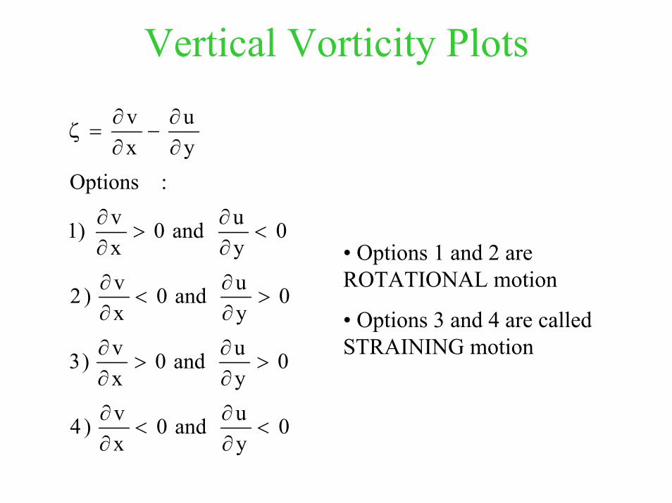
Vertical Vorticity Plots

0yu and 0

xv )4

0yu and 0

xv )3

0yu and 0

xv )2

0yu and 0

xv 1)

:Optionsyu

xv

<∂∂

<∂∂

>∂∂

>∂∂

>∂∂

<∂∂

<∂∂

>∂∂

∂∂

−∂∂

=ζ

• Options 1 and 2 are ROTATIONAL motion

• Options 3 and 4 are called STRAINING motion

Positive Vorticity Negative Vorticity

Cyclones (Northern Hemisphere)Anticyclones (Southern Hemisphere)

Anticyclones (Northern Hemisphere)Cyclones (Southern Hemisphere)

0yu ,0

xv

<∂∂

>∂∂

0yu ,0

xv

>∂∂

<∂∂

y

x

y

x

0yu

xv

>∂∂

−∂∂

=ζ 0yu

xv

<∂∂

−∂∂

=ζ

Primitive Equations in Isobaric Coordinates

1) Material Derivative• Cartesian Coordinates: x, y, z, t

• Isobaric Coordinates: x, y, p, t

DtDz wwhere

zw

yv

xu

tDtD

=

∂∂

+∂∂

+∂∂

+∂∂

=

DtDp where

pyv

xu

tDtD

=ω

∂∂

ω+∂∂

+∂∂

+∂∂

=

2) Pressure Gradient Term

• Any scalar φ can be represented in either coordinate system and the value of φ at a point (x,y,z) is the value of φ in the pressure coordinate system at the point (x,y,p) where z = z(x,y,p,t)

t,p,xt,z,xt,p,x

t,p,yt,z,yt,p,y

t,p,y

xz

zyy

Similarly

xz

zxx

xt

txz

zxy

yxx

xx

:rulechain theUsing)t),t,p,y,x(z,y,x()t,p,y,x(

∂∂

∂φ∂

+∂φ∂

=∂φ∂

∂∂

∂φ∂

+∂φ∂

=∂φ∂

∂∂

∂φ∂

+∂∂

∂φ∂

+∂∂

∂φ∂

+∂∂

∂φ∂

=∂φ∂

φ=φ

α−=∂Φ∂

−∂Φ∂

−=∂∂

ω+∂∂

+∂∂

+∂∂

=

+∂Φ∂

−=∂∂

ω+∂∂

+∂∂

+∂∂

=

α−=∂Φ∂

ρ−

=∂∂

p

fuyp

vyvv

xvu

tv

DtDv

fvxp

uyuv

xuu

tu

DtDu

:as written becan scoordinate isobaricin motion of equations ssfrictionle theTherefore

por

g1

pz

:balancechydrostatiassumed weNow

pz

pz

pz

pz

t,p,yt,z,yt,p,y

t,p,xt,z,xt,p,x

t,p,yt,z,yt,p,y

yyp1

Similarly

xxp1

algeopotenti theis wheregz Using

xz)g(

xp

gzp :balance chydrostati Assuming

xz

zp

xp

xz

zp

xp

xp

:pressure is that assume weIf

xz

zyy

xz

zxx

∂Φ∂

−=∂∂

ρ−

∂Φ∂

−=∂∂

ρ−

Φ=Φ

∂∂

ρ−=∂∂

−

ρ−=∂∂

∂∂

∂∂

=∂∂

−

∂∂

∂∂

+∂∂

=∂∂

φ

∂∂

∂φ∂

+∂φ∂

=∂φ∂

∂∂

∂φ∂

+∂φ∂

=∂φ∂

3) Continuity Equation

It can be shown (see Holton pg 59-60) that the continuity equation in isobaric coordinates is given by:

It should be noted that the continuity equation does not have any reference to the density field, nor does it involve any time derivatives. This is one of the main advantages for using the isobaric coordinate system.

0py

vxu

=∂ω∂

+∂∂

+∂∂

( )

here y

jx

i and ector,velocity v

horizontal the torefers v s,coordinate isobaric torefers psubscript thewhere

0vp

vkfp

vvvt

v

:bygiven thereforearescoordinateisobaricin equationsprimitive ssfrictionle The

ppp

H

p

HpH

pHpHH

⎟⎟⎠

⎞⎜⎜⎝

⎛∂∂

+⎟⎠⎞

⎜⎝⎛∂∂

=∇

=⋅∇

α−=∂Φ∂

×−Φ−∇=∂∂

ω+∇⋅+∂∂

rr

r

r

rrrrr

r

The Omega Equation

• It is useful to combine the vorticity equation and the first law of thermodynamics into a single equation that describes the vertical motion above the surface associated with extratropical cyclones and other types of synoptic weather features

• This equation, which we will now derive, is called the OMEGA equation

• Step 1: Derive vorticity equation on a constant pressure surface:– Proceed as we did before to form the vorticity equation by subtracting ∂/∂y of

the u momentum equation in isobaric coordinates from ∂/∂x of the v momentum equation in isobaric coordinates

– Neglecting the tilting and friction terms– We get:

(1)

where ζp is the relative vorticity on a constant pressure surface,

(2)

• Step 2: Form a geostrophic vorticity:– Using the geostrophic wind relation:

(3)we can obtain the geostrophic vorticity:

(4)

( ) ( )p

ffVt ppp

p

∂ω∂

+ζ=+ζ∇⋅+∂ζ∂ r

p-by replacedbeen has

yv

xu and

yj

xip ∂

ω∂∂∂

+∂∂

∂∂

+∂∂

=∇rr

zkfgv pg ∇×=rr

g2pg z

fgv ζ=∇=×∇

rr

• From (4) the vorticity can be estimated from the curvature of the height contours on a constant pressure analysis

• Substituting (4) into (1), where ζp is set equal to ζg gives:

(5)

• Step 3: Include thermodynamics using the First Law of Thermodynamics

(6)

where Q represents changes in sensible heat of a parcel (diabatic effects). Q can include explicit synoptic-scale phase changes of water as represented by –Ldws, as well as radiative flux divergence and subsynoptic-scale phase changes of water due to cumulus clouds

( ) ( )p

ffvzfg

t ggp2p ∂

ω∂+ζ=+ζ∇⋅+∇

∂∂ rrr

dtlndc

TQ

dc

Tdq dp

pRdT

Tc

dc

p) lnp (lncRlnT ln

ppT Now

pdpR

TdTc

Tdq dp

TTdTc

Tdq

p

ppp

0p

cR

0

pp

p

θ==>

θθ

==>−=θθ

=>

−+=θ=>⎟⎟⎠

⎞⎜⎜⎝

⎛=θ

−==>α

−=

• Equation (6) can be written as:

on (5)

(7)

Notes

• The Omega equation is a second order diagnostic (only spatial derivatives) equation in ω

• It does not require information on the vorticity tendency as with the vorticity equation

• It does not require information on the temperature tendency

• However, the terms on the RHS employ higher-order derivatives than are used in other methods of vertical velocity estimation

easily moreequation Omega theof terms threetheinterpret tofindings theseuse now We

~ w

e thereforand

-w~ : thengradient, pressure and tendency pressure of valuessynoptic lfor typica

gwzpw

zpw

ypv

xpu

tp

DtDp Since

~ therefore

kxsinA~

: thenh, wavelengt theis L where/L2k and constant, a isA wherekxsin Ak

:form wavea has If ).p/ fromdifferent is oft coefficien the

as (7) toobtainedeasily not issolution quantative(although form theof is

(7) of side lefthand that thenote (7),in termsdifferent theof importance theshow To

2

2

22

2222p

2

ω∇

ω

ρ−=∂∂

≅∂∂

+∂∂

+∂∂

+∂∂

==ω

ω−ω∇

ω

π=

−=ω∇

ω∇∂ω∂ω∇

ω∇

r

r

r

rr

r

First Term:Vorticity Advection

ticity.

Second Term: Temperature Advection

[ ] kxBkTV p sin~

:by drepresente becan surface pressureconstant aon re temperatuofadvection theof curvature The

22p −∇⋅∇

rrr

Third Term: Diabatic Heating

An example of diabatic heating on the synoptic scale is deep cumulonimbus activity. An example of diabatic cooling is longwaveradiative flux divergence

Summary• The preceding analysis suggests the following relation between vertical

motion, vorticity, temperature advection and diabatic heating:

• When a combination of terms exist that separately would result in different signs of vertical motion (eg PVA with cold advection), the resultant vertical motion will depend on the relative magnitudes of the individual contributions

• Remember: this relation for vertical motion is only accurate as long as the assumptions used to derive the Omega equation are valid

w > 0 w < 0Positive Vorticity Advection (PVA)

Negative Vorticity Advection (NVA)

Warm Advection Cold Advection

Diabatic Heating Diabatic Cooling

Rules of Thumb for Synoptic AnalysesVorticity Advection • Evaluate at 500 mb

Temperature Advection • Evaluate at 700 mb• At elevations near sea level, also evaluate at 850 mb

Diabatic Heating • Contribution of major importance in synoptic weather patterns (especially cyclogenesis) are areas of deep cumulonimbus• Refer to geostationary satellite imagery for determination of locations of deep convection

General Notes• Mid-term exam: Thursday October 16, 12:10 – 2:10• Includes theory and lab applications, weighted more

heavily toward theory• Derivations are fair game although the following

derivations will NOT be included: virtual temperature, enthalpy, vorticity equation, Omega equation, Q vector form of the Omega equation, and Petterssen’s equation. You must however understand the final form of the various equations, be able to interpret their terms and use these equations in explanations of various weather phenomena

• Bring questions to class next Tuesday

Omega Equation

The Q Vector• Although the Omega Equation has 3 terms that are clearly

interpreted as 3 separate physical processes, in practice there is often a significant amount of cancellation between the terms. Also they are not invariant under a Galilean transformation of the zonal coordinate (adding a constant mean zonal velocity willchange the magnitude of each of the terms without changing the net forcing of vertical motion).

• As a result, an alternative form of the Omega equation, the Q-vector form, has been developed in which the forcing of the vertical motion is expressed in terms of the divergence of the horizontal vector forcing field

• The derivation of the Q-vector Omega equation from Cotton’s notes follows. It is included for completeness and will become more meaningful once the associated approximations and assumptions have been covered in dynamics.

• The Q-vector form of the Omega equation is given by:

• This equation shows that on the f plane vertical motion is forced only by the divergence of Q

• Unlike the traditional form of the Omega equation, the Q-vector form does not have forcing terms that partly cancel.

• The forcing of ω can be represented simply by the pattern of the Q vector

• It is evident from this form of the Omega equation that regions where Q is convergent (divergent) correspond to upward (downward) motion

( )

ion)approximat plane (fconstant a is f and

,,QQ

where

2

0

21

2

22

02

⎟⎟⎠

⎞⎜⎜⎝

⎛∇⋅

∂

∂−∇⋅

∂

∂−==

⋅∇−=∂∂

+∇

Ty

VpRT

xV

pRQ

Qp

f

gg

rrr

rrωωσ

( )

( )

( )

⎟⎟⎠

⎞⎜⎜⎝

⎛

∂∂

×∂∂

−==>

⎟⎟⎠

⎞⎜⎜⎝

⎛∂∂

−∂∂

∂∂

−=⎟⎟⎠

⎞⎜⎜⎝

⎛∂∂−

∂∂

∂∂

−==

∂∂−

=∂∂

⎟⎟⎠

⎞⎜⎜⎝

⎛∂∂

∂∂

∂∂

−=⎟⎟⎠

⎞⎜⎜⎝

⎛∂∂

∂∂

−∂∂

∂∂

−==

⎟⎟⎠

⎞⎜⎜⎝

⎛⎥⎦

⎤⎢⎣

⎡∂∂

∂∂

+∂∂

∂∂

⎥⎦

⎤⎢⎣

⎡∂∂

∂∂

+∂∂

∂∂

=

⎟⎟⎠

⎞⎜⎜⎝

⎛∇⋅

∂∂

−∇⋅∂∂

−==

xV

kyT

pRQ

jxu

ixv

yT

pR

xu

,xv

yT

pRQ,QQ

thereforeyv

xu

But

yv

,xv

yT

pR

yT

yv

pR,

yT

xv

pRQ,QQ

: tosimplified becan expression above then left, on theair cold with isotherm local the toparallel axis-our x place wephysically means what thisunderstand To

yT

yv

xT

yu

pR-,

yT

xv

xT

xu

pR-

TyV

pR,T

xV

pRQ,QQ

thatsawjust weNow

g

gggg21

gg

gggg21

gggg

gg21

rr

rrr

r

rrr

⎟⎟⎠

⎞⎜⎜⎝

⎛

∂∂

×∂∂

−=xV

kyT

pRQ g

rr

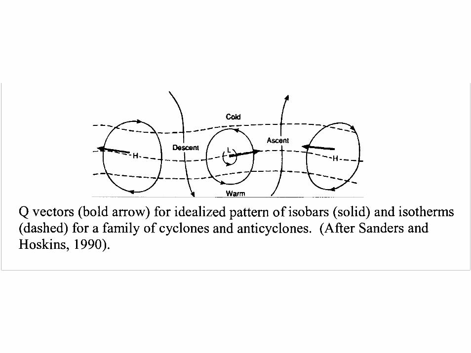
• We can then get the Q-vector by determining the vectorial change of Vg along the isotherm (with cold air on the left), then rotating the resulting change vector by 90° clockwise, and then multiplying the resulting vector by |∂T/∂y|

• In the regions on the map where Q-vectors converge there is rising motion, and in the regions where the Q-vectors diverge there is sinking motion

Petterssen’s Development Equation

• We now derive an equation that gives us information about the change of surface absolute vorticity

• If the vertical advection of absolute vorticity, the tilting term and the solenoidal term are ignored, then the vorticity equation can be written as:

where we assumed that the above equation is valid at the level of nondivergence (~ 500 mb)

• Since, if the wind is in geostrophic balance:

( ) ( ) 0=+∇⋅+∂+∂ fVt

fzpH

z ζζ rr

surface pressure on the wind theis HVr

( )

QpcR

pzgV

pzg

t

:equation Omega theof derivationour in equation following thesaw We

tzfor expressionan need We

p

dp =ωσ−⎟⎟

⎠

⎞⎜⎜⎝

⎛∂∂

∇⋅−⎟⎟⎠

⎞⎜⎜⎝

⎛∂∂

−∂∂

∂∆∂

rr

The Thermal Wind Equation

• The thermal wind equation provides us with information about cold and warm air advection

• Previously we derived the thermal wind equation in Cartesian coordinates – we will now derive the equation using pressure as a vertical coordinate:

zfgkV

:notation vector using written becan which xz

fg v and

yz

fgu

:as written becan scoordinate pressurein windcgeostrophi theof components horizontal The

pg

gg

∇×=

∂∂

=∂∂

−=

rr

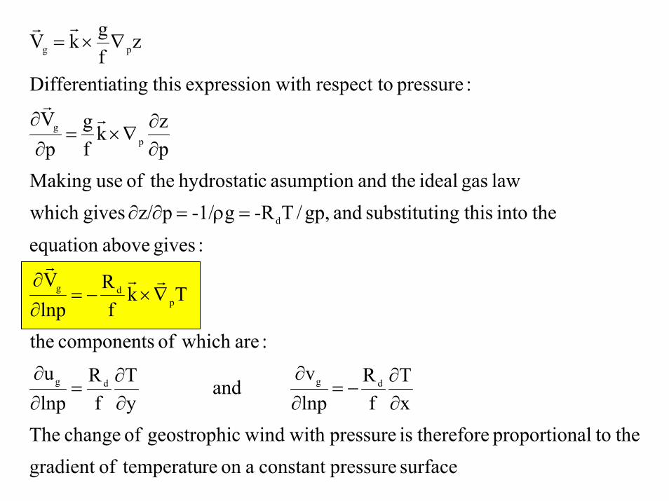
surface pressureconstant aon re temperatuofgradient the toalproportion thereforeis pressure with windcgeostrophi of change The

xT

fR

lnpv

and yT

fR

lnpu

:are which of components the

Tkf

RlnpV

:gives aboveequation theinto thisngsubstituti and ,gp/T-Rg-1/pz/ giveswhich

law gas ideal theandasumption chydrostati theof use Makingpzk

fg

pV

:pressure respect to with expression thisatingDifferenti

zfgkV

dgdg

pdg

d

pg

pg

∂∂

−=∂∂

∂∂

=∂∂

∇×−=∂∂

=ρ=∂∂

∂∂

∇×=∂∂

∇×=

rrr

rr

rr

( )

( )

zkfgV

:as written becan equation wind thermal that themeanswhich

Tppln

gR)z(

:gives p/plng

TRzequation thicknessin theoperation gradient thePerforming

gradient. thicknessa of in terms written be alsocan equation wind thermalThe

WINDTHERMAL thecalled is Vquantity The

pplnTk

fRV

integral. thefrom T take tousedbeen has theoremmean value thewhere

pplnTk

fRVVVplnd

lnpV

:grearrangin and surfaces pressure obetween twequation thisgIntegratin

Tkf

RlnpV

pg

p2

1dp

21d

g

2

1p

dg

p

2

1p

dggg

pln

pln

g

pdg

1p2p

2

1

∆∇×=∆

∇⎟⎟⎠

⎞⎜⎜⎝

⎛=∆∇

=∆

∆

⎟⎟⎠

⎞⎜⎜⎝

⎛∇×=∆=>

∇

⎟⎟⎠

⎞⎜⎜⎝

⎛∇×=∆=−=

∂∂

∇×−=∂∂

∫

rrr

rr

r

rrr

r

rrrrrr

rrr

Implications of the Thermal Wind Relations1) Frontal Strengths

( )

front strong a of

indicative are mb 500at windsstrong small,usually is mb 1000at V Since

front strong V s m 37.5

front moderate s m 37.5 V s m 25.0

front weak s m 25.0 V s m 12.5

front no s m 12.5 V

:Service Weather USby the usefor destablishebeen have criteria following themb 500 and mb 1000 surfaces pressure the Usingfronts. synoptic ofstrength the

classify toused is V equation, thicknesshrough thegradient t etemperatur

horizontal average theof vlaue the torelated is V of magnitude theSince

zfkgV

: thatsawjust We

g

g1-

1-g

1-

1-g

1-

1-g

g

g

pg

→∆<

→≤∆<

→≤∆<

→<∆

∆

∆

∆∇×=∆

r

r

r

r

r

r

rr

r

2) Jet Stream LocationWe also saw that:

As the sign of the synoptic temperature gradient is usually the same up to the tropopause, the geostrophic wind continues to increase with height. Above the tropopause, the temperature gradient reverses sign so that the geostrophic wind decreases with height. The region of strongest geostrophic wind near the tropopause is called the jet stream.

Tkf

Rpln

Vp

dg ∇×−=∂∂ rrr

3) Temperature Advection• The magnitude and direction of the thermal wind can be used to

estimate temperature advection• The thermal wind blows parallel to the isotherms with the warm air

to the right facing downstream in the Northern Hemisphere• Geostrophic winds which rotate counterclockwise (back) with

height are associated with cold advection in the Northern Hemisphere

• Geostrophic winds which rotate clockwise (veer) with height are associated with warm advection in the Northern Hemisphere

• In the Southern Hemisphere the reverse is true• In the case of no temperature advection, only the speed of the

geostrophic wind, not the direction, changes with height. With cold air towards the pole, this requires that the westerlies increase in speed with height with a low-level westerly geostrophic wind. With warm air to the north, the westerlies would decrease with height.

Ta < Tb, P1 > P2

Tkf

Rpln

Vp

dg ∇×−=∂∂ rrr

Potential Vorticity

• Rossby’s (Barotropic) Potential Vorticity • Ertel’s Potential Vorticity • Uses of PV

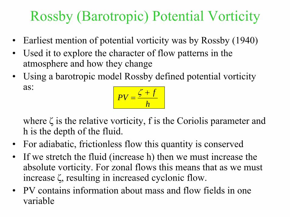
Rossby (Barotropic) Potential Vorticity• Earliest mention of potential vorticity was by Rossby (1940)• Used it to explore the character of flow patterns in the

atmosphere and how they change• Using a barotropic model Rossby defined potential vorticity

as:

where ζ is the relative vorticity, f is the Coriolis parameter and h is the depth of the fluid.

• For adiabatic, frictionless flow this quantity is conserved• If we stretch the fluid (increase h) then we must increase the

absolute vorticity. For zonal flows this means that as we must increase ζ, resulting in increased cyclonic flow.

• PV contains information about mass and flow fields in one variable

hfPV +

=ζ

Ertel’s Potential Vorticity• A more general definition for potential vorticity was

found by Ertel (1942)• Ertel used a three-dimensional vector form of the

equation of motion for frictionless flow, the thermodynamic equation for adiabatic motion and the mass continuity equation and derived the following conservation principle:

where ρ is the density, ζa is the absolute vorticity vector, and φ is any conservative thermodynamic variable. In meteorology, φ is typically taken to be potential temperature

01=⎟⎟

⎠

⎞⎜⎜⎝

⎛∇⋅ ϕζ

ρ

raDt

D

• Using potential temperature as our thermodynamic variable, we then get:

• The conserved quantity

is called Ertel’s potential vorticity

• Note: the only assumptions are for frictionless, adiabatic flowcompared to barotropic model assumptions made by Rossby

• Ertel’s theory can be extended to include diabatic and frictional effects (see Cotton’s notes for derivation if you are interested)

01=⎟⎟

⎠

⎞⎜⎜⎝

⎛∇⋅= θζ

ρ

raDt

DDtDP

θζρ

∇⋅=r

aP 1

• Units of PV: K kg-1 m2 s-1

• In meteorology, the following definition is typically used:– 1 PVU = 10-6 K kg-1 m2 s-1 where PVU stands for

potential vorticity units– Values of IPV less than ~1.5 PVU are usually

associated with tropospheric air– IPV values larger than 1.5 PVU are usually

associated with stratospheric air

• Isentropic Potential Vorticity (IPV) is given by:

where ζθ is the vertical component of relative vorticity evaluated on an isentropic surface

• Potential vorticity is therefore the product of the absolute vorticity and the static stability. If the static stability is increased (i.e., if ∂θ/∂p is made more negative), absolute vorticity (which is positive) is decreased and vice versa.

• The “potential” in potential vorticity relates to the value the relative vorticity would have if a parcel is moved adiabatically to a standard latitude and static stability.

( )4847648476

stability Static vorticity

Absolute

const)p

g(fP =∂θ∂

−+ζ= θ

• IPV is defined with a minus sign so that its value is normally positive in the Northern Hemisphere

• The expression on the previous slide shows that potential vorticity is conserved following the motion in adiabatic, frictionless flow

• PV is always in some sense a measure of the ratio of the absolute vorticity to the effective depth of the vortex. In the expression on the previous slide, the effective depth is just the distance between isentropic surfaces measured in pressure units (-∂θ/∂p)

• The conservation of PV is a powerful constraint on large-scale motions of the atmosphere

( ) constp

gfP =∂∂

−+= )( θζθ

A cylindrical column of air moving adiabatically, conserving potential vorticity

Ref: Holton

Uses of PV1. Surface cyclones have been found to be

accompanied by a positive PV anomaly (high PV air relative to the environment) aloft

2. Tracer of stratospheric air– As PV is a function of static stability, regions with

strong static stability should also be regions of high PV

– The stratosphere has been recognized as a possible source region or reservoir of high-PV air – above the tropopause θ rapidly increases with height and hence so does PV

– PV values larger than 1.5 PVU are usually associated with stratospheric air

3. Indicator or troughs and ridges, as well as closed lows and highs

- Tongues of high-IPV(low-IPV), stratospheric (tropospheric) air that extend equatorward (poleward) from the high-IPV reservoir (low-IPV troposphere) are associated with troughs (ridges) in the height field and cyclonic (anticyclonic) flow

– Isolated regions of stratospheric IPV that are situated equatorward from the reservoir tend to be associated with troughs or closed lows in the height field and associated cyclonic flow

Ertel’s PV (PVU) evaluated on the 325K surface (left) on (a) 1200 UTC, May 16, (b) 1200 UTC, May 17, and (c) 1200 UTC, May 18, 1989. Corresponding 500 mb height contours, temperature and dew-point depression (°C). Ref: Bluestein

4. Lee Cyclogenesis

• Westerly Flow- Suppose that upstream of the mountain barrier flow is

a uniform zonal flow => ζ=0- If the flow is adiabatic, each column of air is confined

between the potential temperature surfaces θ0 and θ0+δθ as it crosses the mountain

- Potential temperature surface θ0 near the ground approximately follows the contours of the ground. A potential temperature surface θ0 + δθ several kilometers above the ground will also be deflected vertically, however, the vertical displacement at upper levels is spread horizontally and has less displacement in the vertical than that near the ground

- Due to the vertical displacement of the upper-level isentropic surfaces there is a vertical stretching of air columns upstream of the topographic barrier => causes -∂θ/∂p to decrease=> ζ must become positive to conserve PV=> air column turns cyclonically as it approaches the topographic barrier=> the cyclonic curvature causes a poleward drift so that f also increases which reduces the change in ζrequired for PV conservation

- As the column begins to cross the barrier its vertical extent decreases=> relative vorticity must then become negative=> air column will acquire anticyclonic vorticity and move southward

- Once the air column has passed over the mountain and returned to its original depth it will be south of its original latitude so that f will be smaller and the relative vorticity must be positive=> trajectory must have cyclonic curvature=> column will be deflected poleward=> when parcel reaches its original latitude it will still have a poleward velocity component and will continue poleward gradually acquiring anticyclonic curvature until its direction is reversed=> parcel will then move downstream conserving PV by following a wave-like trajectory in the horizontal plane

- A steady westerly flow over a large-scale mountain barrier will therefore result in a cyclonic flow pattern immediately to the east of the barrier (called the lee side trough) followed by an alternating series of ridges and troughs

Schematic view of westerly flow over a topographic barrier: (a) the depth of the fluid column as a function of x and (b) the trajectory of a parcel in the x,y plane Ref: Holton

• Easterly Flow– Similar reasoning may be applied to obtain the effects

of a large topographic barrier on a purely zonal easterly flow

– There is a dramatic difference between easterly and westerly flow over large-scale topographic barriers

– In the westerly wind case the barrier generates wavelike disturbances in the streamlines that extend downwind from the barrier

– In the easterly wind case the disturbance in the streamlines damps out away from the barrier

– The differences are due to the dependence of the Coriolis parameter on latitude

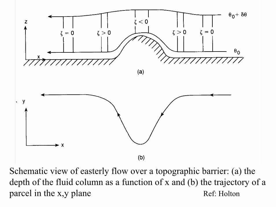
Schematic view of easterly flow over a topographic barrier: (a) the depth of the fluid column as a function of x and (b) the trajectory of a parcel in the x,y plane Ref: Holton

Midterm Exam: General Notes

• Mid-term exam: Thursday October 16, 12:10 – 2:10• Includes theory and lab applications, weighted more

heavily toward theory• Derivations are fair game although the following

derivations will NOT be included: virtual temperature, enthalpy, vorticity equation, Omega equation, Q vector form of the Omega equation, and Petterssen’s equation.

• You must however understand the final form of the various equations, know what basic equations and assumptions are used in the derivations, be able to interpret their terms and use these equations in explanations of various weather phenomena

• Bring colored pencils• No programmable calculators

Chapter 2 Outline

• The primary variables• Instrumentation used to measure the

primary variables• Remote sensing

– Electromagnetic spectrum and associated laws– Instrumentation: satellite, radar, wind profilers

Chapter 3 Outline• The Gas Laws

– Ideal gas law: general, dry air, water vapor– Universal Gas constant, gas constant for dry air and water vapor– Virtual temperature

• Hydrostatic Equation• Geopotential and geopotential height

– High and low pressure, ridges and troughs• Thickness

– Thickness / Hypsometric equation– Warm and cold core systems– Uses of thickness: frontal location, rain-snow line, warm or cold

air advection• First Law of Thermodynamics

– Various forms of the first law– Joule’s law

• Specific Heats– At constant volume– At constant pressure

• Enthaply• Potential temperature• Dry Adiabatic Lapse Rate

• Water vapor and moisture parameters:– Mixing ratio– Specific humidity– Saturation vapor pressure with respect to liquid water and ice– Saturation mixing ratios– Dew point temperature and frost point temperature– Lifting condensation level– Wet bulb temperature

• Saturated Adiabatic Lapse Rate• Equivalent potential temperature• Static stability• Conditional instability• Convective or potential instability

Chapter 4 Outline• Coordinate Systems

– Velocity Components– Pressure as a vertical coordinate– Other vertical coordinates– Natural coordinates

• Apparent Forces– Coriolis Force– Effective gravity

• Thermal Wind• Balance Winds

– Geostrophic, gradient, cyclostrophic, friction

• Continuity Equation– Material derivative form, flux form,– Incompressibility, convergence, divergence, level of

nondivergence, vertical motion– Pressure tendency equation

• Baroclinity and barotropy• Vorticity

– Components– Absolute and relative vorticity– Vorticity equation and interpretation of all terms– Rotational and shear vorticity

• Omega Equation• Q vectors• Petterssen’s Developmental Equation• Potential Vorticity