asymptotic properties of a robust variance matrix ...d.sul/econo2/hansen-2007-joe-panelhac.pdf ·...
TRANSCRIPT

ARTICLE IN PRESS
Journal of Econometrics 141 (2007) 597–620
0304-4076/$ -
doi:10.1016/j
E-mail ad
www.elsevier.com/locate/jeconom
Asymptotic properties of a robust variance matrixestimator for panel data when T is large
Christian B. Hansen
University of Chicago, Graduate School of Business, 5807 South Woodlawn Ave., Chicago, IL 60637, USA
Available online 20 November 2006
Abstract
I consider the asymptotic properties of a commonly advocated covariance matrix estimator for
panel data. Under asymptotics where the cross-section dimension, n, grows large with the time
dimension, T, fixed, the estimator is consistent while allowing essentially arbitrary correlation within
each individual. However, many panel data sets have a non-negligible time dimension. I extend the
usual analysis to cases where n and T go to infinity jointly and where T !1 with n fixed. I provide
conditions under which t and F statistics based on the covariance matrix estimator provide valid
inference and illustrate the properties of the estimator in a simulation study.
r 2007 Elsevier B.V. All rights reserved.
JEL classification: C12; C13; C23
Keywords: Panel; Heteroskedasticity; Autocorrelation; Robust; Covariance matrix
1. Introduction
The use of heteroskedasticity robust covariance matrix estimators, cf. White (1980), incross-sectional settings and of heteroskedasticity and autocorrelation consistent (HAC)covariance matrix estimators, cf. Andrews (1991), in time series contexts is extremelycommon in applied econometrics. The popularity of these robust covariance matrixestimators is due to their consistency under weak functional form assumptions. Inparticular, their use allows the researcher to form valid confidence regions about a set ofparameters from a model of interest without specifying an exact process for thedisturbances in the model.
see front matter r 2007 Elsevier B.V. All rights reserved.
.jeconom.2006.10.009
dress: [email protected].

ARTICLE IN PRESSC.B. Hansen / Journal of Econometrics 141 (2007) 597–620598
With the increasing availability of panel data, it is natural that the use of robustcovariance matrix estimators for panel data settings that allow for arbitrary withinindividual correlation are becoming more common. A recent paper by Bertrand et al.(2004) illustrated the pitfalls of ignoring serial correlation in panel data, finding through asimulation study that inference procedures which fail to account for within individualserial correlation may be severely size distorted. As a potential resolution of this problem,Bertrand et al. (2004) suggest the use of a robust covariance matrix estimator proposed byArellano (1987) and explored in Kezdi (2002) which allows arbitrary within individualcorrelation and find in a simulation study that tests based on this estimator of thecovariance parameters have correct size.One drawback of the estimator of Arellano (1987), hereafter referred to as the
‘‘clustered’’ covariance matrix (CCM) estimator, is that its properties are only known inconventional panel asymptotics as the cross-section dimension, n, increases with the timedimension, T, fixed. While many panel data sets are indeed characterized by large n andrelatively small T, this is not necessarily the case. For example, in many differences-in-differences and policy evaluation studies, the cross-section is composed of states and thetime dimension of yearly or quarterly (or occasionally monthly) observations on each statefor 20 or more years.In this paper, I address this issue by exploring the theoretical properties of the CCM
estimator in asymptotics that allow n and T to go to infinity jointly and in asymptoticswhere T goes to infinity with n fixed. I find that the CCM estimator, appropriatelynormalized, is consistent without imposing any conditions on the rate of growth of T
relative to n even when the time series dependence between the observations within eachindividual is left unrestricted. In this case, both the OLS estimator and the CCM estimatorconverge at only the
ffiffiffinp
-rate, essentially because the only information is coming fromcross-sectional variation. If the time series process is restricted to be strongly mixing, Ishow that the OLS estimator is
ffiffiffiffiffiffiffinTp
-consistent but that, because high lags are not downweighted, the robust covariance matrix estimator still converges at only the
ffiffiffinp
-rate. Thisbehavior suggests, as indicated in the simulations found in Kezdi (2002), that it is the n
dimension and not the size of n relative to T that matters for determining the properties ofthe CCM estimator.It is interesting to note that the limiting behavior of bb changes ‘‘discontinuously’’ as the
amount of dependence is limited. In particular, the rate of convergence of bb changes fromffiffiffinp
in the ‘‘no-mixing case’’ toffiffiffiffiffiffiffinTp
when mixing is imposed. However, despite thedifference in the limiting behavior of bb, there is no difference in the behavior of standardinference procedures based on the CCM estimator between the two cases. In particular, thesame t and F statistics will be valid in either case (and in the n!1 with T fixed case)without reference to the asymptotics or degree of dependence in the data.I also derive the behavior of the CCM estimator as T !1 with n fixed, where I find the
estimator is not consistent but does have a limiting distribution. This result corresponds toasymptotic results for HAC estimators without truncation found in recent work by Kieferand Vogelsang (2002, 2005), Phillips et al. (2003), and Vogelsang (2003). While the limitingdistribution is not proportional to the true covariance matrix in general, it is proportionalto the covariance matrix in the important special case of iid data across individuals,1
1Note that this still allows arbitrary correlation and heteroskedasticity within individuals, but restricts that the
pattern is the same across individuals.

ARTICLE IN PRESSC.B. Hansen / Journal of Econometrics 141 (2007) 597–620 599
allowing construction of asymptotically pivotal statistics in this case. In fact, in this case,the standard t-statistic is not asymptotically normal but converges in distribution to arandom variable which is exactly proportional to a tn�1 distribution. This behaviorsuggests the use of the tn�1 for constructing confidence intervals and tests when the CCMestimator is used as a general rule, as this will provide asymptotically correct critical valuesunder any asymptotic sequence.
I then explore the finite sample behavior of the CCM estimator and tests based upon itthrough a short simulation study. The simulation results indicate that tests based on therobust standard error estimates generally have approximately correct size in seriallycorrelated panel data even in small samples. However, the standard error estimatesthemselves are considerably more variable than their counterparts based on simpleparametric models. The bias of the simple parametric estimators is also typically smaller inthe cases where the parametric model is correct, suggesting that these standard errorestimates are likely preferable when the researcher is confident in the form of the errorprocess. In the simulation, I also explore the behavior of an analog of White’s (1980) directtest for heteroskedasticity proposed by Kezdi (2002).2 The results indicate the performanceof the test is fairly good for moderate n, though it is quite poor when n is small. Thissimulation behavior suggests that this test may be useful for choosing between the use ofrobust standard error estimates and standard errors estimated from a more parsimoniousmodel when n is reasonably large.
The remainder of this paper is organized as follows. In Section 2, I present the basicframework and the estimator and test statistics that will be considered. The asymptoticproperties of these estimators are collected in Section 3, and Section 4 contains a discussionof a Monte Carlo study assessing the finite sample performance of the estimators in simplemodels. Section 5 concludes.
2. A heteroskedasticity–autocorrelation consistent covariance matrix estimator for panel
data
Consider a regression model defined by
yit ¼ x0itbþ �it, (1)
where i ¼ 1; . . . ; n indexes individuals, t ¼ 1; . . . ;T indexes time, xit is a k � 1 vector ofobservable covariates, and �it is an unobservable error component. Note that thisformulation incorporates the standard fixed effects model as well as models which includeother covariates that enter the model with individual specific coefficients, such asindividual specific time trends, where these covariates have been partialed out. In thesecases, the variables xit, yit, and �it should be interpreted as residuals from regressions of x�it,y�it, and ��it on an auxiliary set of covariates z�it from the underlying modely�it ¼ x�
0
it bþ z�0
it gþ ��it. For example, in the fixed effects model, Z� is a matrix of dummy
variables for each individual and g is a vector of individual specific fixed effects. In thiscase, xit ¼ x�it � ð1=TÞ
PTt¼1 x�it, and yit and �it are defined similarly. Alternatively, xit, yit,
and �it could be interpreted as variables resulting from other transformations which
2Solon and Inoue (2004) offers a different testing procedure for detecting serial correlation in fixed effects panel
models. See also Bhargava et al. (1982), Baltagi and Wu (1999), Wooldridge (2002, pp. 275, 282–283), and
Drukker (2003).

ARTICLE IN PRESSC.B. Hansen / Journal of Econometrics 141 (2007) 597–620600
remove the nuisance parameters from the equation, such as first-differencing to remove thefixed effects. In what follows, all properties are given in terms of the transformed variablesfor convenience. Alternatively, conditions could be imposed on the underlying variablesand the properties derived as T !1 as in Hansen (2006).3
Within each individual, the equations defined by (1) may be stacked and represented inmatrix form as
yi ¼ xibþ �i, (2)
where yi is a T � 1 vector of individual outcomes, xi is a T � k vector of observed covariates,and �i is a T � 1 vector of unobservables affecting the outcomes yi with E½�i�0ijxi� ¼ Oi. The
OLS estimator of b from Eq. (2) may then be defined as bb ¼ ðPni¼1 x0ixiÞ
�1Pni¼1 x0iyi. The
properties of bb as n!1 with T fixed are well known. In particular, under regularity
conditions,ffiffiffinpðbb� bÞ is asymptotically normal with covariance matrix Q�1WQ�1 where
Q ¼ limn ð1=nÞPn
i¼1 E½x0ixi� and W ¼ limn ð1=nÞ
Pni¼1 E½x
0iOixi�.
The problem of robust covariance matrix estimation is then estimating W withoutimposing a parametric structure on the Oi. In this paper, I consider the estimator suggestedby Arellano (1987) which may be defined as
bW ¼ 1
nT
Xn
i¼1
x0ib�ib�0ixi, (3)
where b�i ¼ yi � xibb are OLS residuals from Eq. (2). This estimator is an appealing
generalization of White’s (1980) heteroskedasticity consistent covariance matrix estimatorthat allows for arbitrary intertemporal correlation patterns and heteroskedasticity acrossindividuals.4 The estimator is also appealing in that, unlike HAC estimators for time seriesdata, its implementation does not require the selection of a kernel or bandwidth parameter.The properties of bW under conventional panel asymptotics where n!1 with T fixed arewell-established. In the remainder of this paper, I extend this analysis by considering theproperties of bW under asymptotic sequences where T !1 as well.
The chief reason for interest in the CCM estimator is for performing inference about bb.Suppose
ffiffiffiffiffiffiffiffidnT
pðbb� bÞ!
dNð0;BÞ and define an estimator of the asymptotic variance of bb as
ð1=dnT ÞbB where bB!p B. The following estimator of the asymptotic variance of bb based onbW is used throughout the remainder of the paper:
dAvarðbbÞ ¼ Xn
i¼1
x0ixi
!�1ðnT bW Þ Xn
i¼1
x0ixi
!�1
¼Xn
i¼1
x0ixi
!�1 Xn
i¼1
x0ib�ib�0ixi
! Xn
i¼1
x0ixi
!�1. ð4Þ
3This is especially relevant in Theorem 3 where the mixing conditions will not hold for the transformed variables
if, for example, the transformation is to remove fixed effects by differencing out the individual means. Hansen
(2006) provides conditions on the untransformed variables which will cover this case in a different but related
context. This approach complicates the proof and notation and is not pursued here.4It does, however, ignore the possibility of cross-sectional correlation, and it will be assumed that there is no
cross-sectional correlation for the remainder of the paper.

ARTICLE IN PRESSC.B. Hansen / Journal of Econometrics 141 (2007) 597–620 601
In addition, for testing the hypothesis Rb ¼ r for a q� k matrix R with rank q, the usual t
(for R a 1� k vector) and Wald statistics can be defined as
t� ¼
ffiffiffiffiffiffiffinTpðRbb� rÞffiffiffiffiffiffiffiffiffiffiffiffiffiffiffiffiffiffiffiffiffiffiffiffiffiffiffiffiffiffi
R bQ�1 bW bQ�1R0q (5)
and
F� ¼ nTðRbb� rÞ0½R bQ�1 bW bQ�1R0��1ðRbb� rÞ, (6)
respectively, where bW is defined above and bQ ¼ ð1=nTÞPn
i¼1 x0ixi. In Section 3, I verify
that, despite differences in the limiting behavior of bb, t�!dNð0; 1Þ, F�!
dw2q, and dAvarðbbÞ is
valid for estimating the asymptotic variance of bb as n!1 regardless of the behavior of T.
I also consider the behavior of t� and F� as T !1 with n fixed. In this case, bW is notconsistent for W but does have a limiting distribution; and when the data are iid across i,5 I
show that t�!dðn=ðn� 1ÞÞ1=2tn�1 and that F� is asymptotically pivotal and so can be used
to construct valid tests. This behavior suggests that inference using ðn=ðn� 1ÞÞ bW andforming critical values using a tn�1 distribution will be valid regardless of the asymptoticsequence considered.
It is worth noting that the estimator bW has also been used extensively in multilevelmodels to account for the presence of correlation between individuals within cells; cf.Liang and Zeger (1986) and Bell and McCaffrey (2002). For example, in a schooling study,one might have data on individual outcomes where the individuals are grouped intoclasses. In this case, the cross-sectional unit of observation could be defined as the class,and arbitrary correlation between all individuals within each class could be allowed. In thiscase, one would expect the presence of a classroom specific random effect resulting inequicorrelation between all individuals within a class. While this would clearly violate themixing assumptions imposed in obtaining the asymptotic behavior as T !1 with n fixed,it would not invalidate the use of bW for inference about b in cases where n and T go toinfinity jointly.
In addition to being useful for performing inference about bb, bW may also be used to testthe specification of simple parametric models of the error process.6 Such a test may beuseful for a number of reasons. If a parametric model is correct, the estimates of thevariance of bb based on this model will tend to behave better than the estimates obtainedfrom bW . In particular, parametric estimates of the variance of bb will often be considerablyless variable and will typically converge faster than estimates made using bW ; and if theparametric model is deemed to be adequate, this model may be used to perform FGLSestimation. The FGLS estimator is asymptotically more efficient than the OLS estimator,and simulation evidence in Hansen (2006) suggests that the efficiency gain to using FGLSover OLS in serially correlated panel data may be substantial.
5Note that this still allows arbitrary correlation and heteroskedasticity within individuals but restricts that the
pattern is the same across individuals.6The test considered is a straightforward generalization of the test proposed by White (1980) for
heteroskedasticity and was suggested in the panel context by Kezdi (2002).
ARTICLE IN PRESSC.B. Hansen / Journal of Econometrics 141 (2007) 597–620602
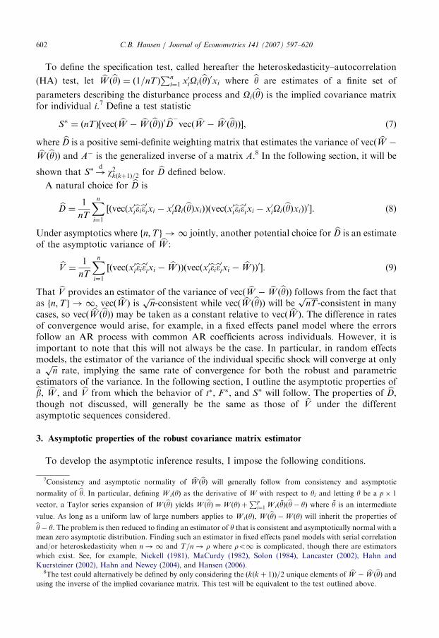
To define the specification test, called hereafter the heteroskedasticity–autocorrelation
(HA) test, let bW ðbyÞ ¼ ð1=nTÞPn
i¼1 x0iOiðbyÞ0xi where by are estimates of a finite set of
parameters describing the disturbance process and OiðbyÞ is the implied covariance matrix
for individual i.7 Define a test statistic
S� ¼ ðnTÞ½vecð bW � bW ðbyÞÞ0 bD�vecð bW � bW ðbyÞÞ�, (7)
where bD is a positive semi-definite weighting matrix that estimates the variance of vecð bW �bW ðbyÞÞ and A� is the generalized inverse of a matrix A.8 In the following section, it will be
shown that S�!dw2kðkþ1Þ=2 for bD defined below.
A natural choice for bD is
bD ¼ 1
nT
Xn
i¼1
½ðvecðx0ib�ib�0ixi � x0iOiðbyÞxiÞÞðvecðx
0ib�ib�0ixi � x0iOið
byÞxiÞÞ0�. (8)
Under asymptotics where fn;Tg ! 1 jointly, another potential choice for bD is an estimateof the asymptotic variance of bW :
bV ¼ 1
nT
Xn
i¼1
½ðvecðx0ib�ib�0ixi � bW ÞÞðvecðx0ib�ib�0ixi � bW ÞÞ0�. (9)
That bV provides an estimator of the variance of vecð bW � bW ðbyÞÞ follows from the fact thatas fn;Tg ! 1, vecð bW Þ is ffiffiffi
np
-consistent while vecð bW ðbyÞÞ will be ffiffiffiffiffiffiffinTp
-consistent in manycases, so vecð bW ðbyÞÞ may be taken as a constant relative to vecð bW Þ. The difference in ratesof convergence would arise, for example, in a fixed effects panel model where the errorsfollow an AR process with common AR coefficients across individuals. However, it isimportant to note that this will not always be the case. In particular, in random effectsmodels, the estimator of the variance of the individual specific shock will converge at onlya
ffiffiffinp
rate, implying the same rate of convergence for both the robust and parametricestimators of the variance. In the following section, I outline the asymptotic properties ofbb, bW , and bV from which the behavior of t�, F�, and S� will follow. The properties of bD,though not discussed, will generally be the same as those of bV under the differentasymptotic sequences considered.
3. Asymptotic properties of the robust covariance matrix estimator
To develop the asymptotic inference results, I impose the following conditions.
7Consistency and asymptotic normality of bW ðbyÞ will generally follow from consistency and asymptotic
normality of by: In particular, defining W iðyÞ as the derivative of W with respect to yi and letting y be a p� 1
vector, a Taylor series expansion of W ðbyÞ yields W ðbyÞ ¼W ðyÞ þPp
i¼1 W iðyÞðby� yÞ where y is an intermediate
value. As long as a uniform law of large numbers applies to W iðyÞ, W ðbyÞ �W ðyÞ will inherit the properties ofby� y. The problem is then reduced to finding an estimator of y that is consistent and asymptotically normal with a
mean zero asymptotic distribution. Finding such an estimator in fixed effects panel models with serial correlation
and/or heteroskedasticity when n!1 and T=n! r where ro1 is complicated, though there are estimators
which exist. See, for example, Nickell (1981), MaCurdy (1982), Solon (1984), Lancaster (2002), Hahn and
Kuersteiner (2002), Hahn and Newey (2004), and Hansen (2006).8The test could alternatively be defined by only considering the ðkðk þ 1ÞÞ=2 unique elements of bW � bW ðbyÞ and
using the inverse of the implied covariance matrix. This test will be equivalent to the test outlined above.

ARTICLE IN PRESSC.B. Hansen / Journal of Econometrics 141 (2007) 597–620 603
Assumption 1. fxi; �ig are independent across i, and E½�i�0ijxi� ¼ Oi.
Assumption 2. QnT ¼ E½Pn
i¼1ðx0ixi=nTÞ� is uniformly positive definite with constant limit Q
where limits are taken as n!1 with T fixed in Theorem 1, as fn;Tg ! 1 in Theorems 2and 3, and as T !1 with n fixed in Theorem 4.
In addition, I impose either Assumption 3(a) or Assumption 3(b) depending on thecontext.
Assumption 3.
(a)
9N
4.1 c
E½�ijxi� ¼ 0.
(b) E½xit�it� ¼ 0.Assumptions 1–3 are quite standard for panel data models. Assumption 1 imposesindependence across individuals, ruling out cross-sectional correlation, but leaves the timeseries correlation unconstrained and allows general heterogeneity across individuals.Assumption 2 is a standard full rank condition, and the restriction that QnT has a constantlimit could be relaxed at the cost of more complicated notation. Assumption 3 imposesthat one of two orthogonality conditions is satisfied. Assumption 3(b) imposes that xit
and �it are uncorrelated and is weaker than the strict exogeneity imposed in Assump-tion 3(a). Assumption 3(a) is stronger than necessary, but it simplifies the proof of asymp-totic normality of bW and consistency of bV . In addition, Assumption 3(a) would typicallybe imposed in fixed effects models.9
The first theorem, which is stated here for completeness, collects the properties of bb andbW in asymptotics where n!1 with T fixed.
Theorem 1. Suppose the data are generated by model (1), that Assumptions 1 and 2 are
satisfied, and that n!1 with T fixed.
(i)
If Assumption 3(b) holds and Ejxithj4þdoDo1 and Ej�itj4þdoDo1 for some d40,then ffiffiffiffiffiffiffi
nTpðbb� bÞ!
dQ�1N 0;W ¼ lim
n
1
nT
Xn
i¼1
E½x0iOixi�
!,
and bW!p W .
(ii)
In addition, if Assumption 3(a) holds and Ejxithj8þdoDo1 and Ej�itj8þdoDo1 for
some d40, thenffiffiffiffiffiffiffinTp½vecð bW �W Þ�
!dN 0;V ¼ lim
n
1
nT
Xn
i¼1
E½ðvecðx0i�i�0ixi �W ÞÞðvecðx0i�i�
0ixi �W ÞÞ0�
!,
ote that a balanced panel has also implicitly been assumed. All of the results with the exception of Corollary
ould be extended to accommodate unbalanced panels at the cost of more complicated notation.

ARTICLE IN PRESS
10
dime
Theo
the s
with
C.B. Hansen / Journal of Econometrics 141 (2007) 597–620604
and bV!p V .
ark 3.1. It follows from Theorem 1(i) that the asymptotic variance of bb can be
Remestimated using (4) since
dAvarðbbÞ ¼ Xn
i¼1
x0ixi
!�1Xn
i¼1
x0ib�ib�0ixi
Xn
i¼1
x0ixi
!�1
¼1
nT
1
nT
Xn
i¼1
x0ixi
!�1 bW 1
nT
Xn
i¼1
x0ixi
!�1¼
1
nTbQ�1 bW bQ�1,
where bQ�1 bW bQ�1!p Q�1WQ�1. It also follows immediately from the definitions of t� and
F� in Eqs. (5) and (6) and Theorem 1(i) that, under the null hypothesis, t�!dNð0; 1Þ and
F�!dw2q. Similarly, using Theorem 1(ii) and assuming bW ðbyÞ has properties similar to those
of bW , it will follow that the HA test statistic, S�, formed using bD defined above converges
in distribution to a w2kðkþ1Þ=2 under the null hypothesis.
Theorem 1 verifies that bb and bW are consistent and asymptotically normal as n!1
with T fixed without imposing any restrictions on the time series dimension. In thefollowing results, I consider alternate asymptotic approximations under the assumptionthat both n and T are going to infinity.10 In these cases, consistency and asymptoticnormality of suitably normalized versions of bW are established under weak conditions.Theorem 2, given immediately below, covers the case where n and T are going to infinity
and there is not weak dependence in the time series. In particular, the results of Theorem 2are only interesting in the case where W ¼ limn;T ð1=nT2Þ
Pni¼1 E½x
0iOixi�40. Perhaps the
leading case where this behavior would occur is in a model where �it includes an individualspecific random effect that is uncorrelated to xit and the estimated model does not includean individual specific effect. In this case, all observations for a given individual will beequicorrelated, and the condition given above will hold. Theorem 3, given followingTheorem 2, covers the case where there is mixing in the time series.
Theorem 2. Suppose the data are generated by model (1), that Assumptions 1 and 2 are
satisfied, and that fn;Tg ! 1 jointly.
(i)
If Assumption 3(b) holds and Ejxithj4þdoDo1 and Ej�itj4þdoDo1 for some d40,then
ffiffiffinpðbb� bÞ!
dQ�1Nð0;W ¼ lim
n;T
1
nT2
Xn
i¼1
E½x0iOixi�Þ,
One could also consider sequential limits in which one takes limits as n or T goes to infinity with the other
nsion fixed and then lets the other dimension go to infinity. It could be shown that under the conditions of
rem 2 and appropriate normalizations sequential limits taken first with respect to either n or T would yield
ame results as the joint limit. Similarly, under the conditions of Theorem 3, the sequential limits taken first
respect to either n or T would produce the same results as the joint limit.

ARTICLE IN PRESSC.B. Hansen / Journal of Econometrics 141 (2007) 597–620 605
and bW=T!p
W .
(ii)
In addition, if Assumption 3(a) holds and Ejxithj8þdoDo1 and Ej�itj8þdoDo1 for
some d40, thenffiffiffinp½vecð bW=T �W Þ�
!dN 0;V ¼ lim
n;T
1
nT4
Xn
i¼1
E½ðvecðx0i�i�0ixi �W ÞÞðvecðx0i�i�
0ixi �W ÞÞ0�
!,
and bV=T3!p
V .
Remark 3.2. It is important to note that the results presented in Theorem 2 are notinteresting in the setting where the fj; kg element of Oi becomes small when jj � kj is largesince in these circumstances ð1=nT2Þ
Pni¼1 E½x
0iOixi� ! 0. Theorem 3 presents results which
are relevant in this case.
Remark 3.3. Theorem 2 verifies consistency and asymptotic normality of both bb and bWwhile imposing essentially no constraints on the time series dependence in the data. Thelarge cross-section effectively allows the time series dimension to be ignored even when T islarge. However, without constraints on the time series, bb is
ffiffiffinp
-consistent, notffiffiffiffiffiffiffinTp
-consistent. Intuitively, the slower rate of convergence is due to the fact that there may belittle information contained in the time series since it is allowed to be arbitrarily dependent.
Remark 3.4. The fact that bb and bW are notffiffiffiffiffiffiffinTp
-consistent will not affect practicalimplementation of inference about bb. In particular, the estimate of the asymptotic variance
of bb based on Eq. (4) is
dAvarðbbÞ ¼ Xn
i¼1
x0ixi
!�1Xn
i¼1
x0ib�ib�0ixi
Xn
i¼1
x0ixi
!�1
¼1
n
1
nT
Xn
i¼1
x0ixi
!�1ð bW=TÞ
1
nT
Xn
i¼1
x0ixi
!�1¼
1
nbQ�1ð bW=TÞ bQ�1,
where bQ�1ð bW=TÞ bQ�1!p Q�1WQ�1: The t-statistic defined in Eq. (5) may also be expressedas
t� ¼
ffiffiffiffiffiffiffinTpðRbb� rÞffiffiffiffiffiffiffiffiffiffiffiffiffiffiffiffiffiffiffiffiffiffiffiffiffiffiffiffiffiffi
R bQ�1 bW bQ�1R0q
¼
ffiffiffinpðRbb� rÞffiffiffiffiffiffiffiffiffiffiffiffiffiffiffiffiffiffiffiffiffiffiffiffiffiffiffiffiffiffiffiffiffiffiffiffiffiffiffiffi
R bQ�1ð bW=TÞ bQ�1R0q
which converges in distribution to a Nð0; 1Þ random variable under the null hypothesis,
Rb ¼ r, by Theorem 2(i). Similarly, it follows that F�!dw2q under the null. Finally, the HA

ARTICLE IN PRESSC.B. Hansen / Journal of Econometrics 141 (2007) 597–620606
test statistic, S�, defined above also satisfies
S� ¼ ðnTÞ½vecð bW � bW ðbyÞÞ0 bD� vecð bW � bW ðbyÞÞ�¼ n½vecð bW=T � bW ðbyÞ=TÞ0ð bD=T3Þ
� vecð bW=T � bW ðbyÞ=TÞ�,
which converges in distribution to a w2kðkþ1Þ=2 under the conditions of the theorem and the
additional assumption that bW ðbyÞ behaves similarly to bV .
The previous theorem establishes the properties of bb and the robust variance matrixestimator as n and T go to infinity jointly without imposing restrictions on the time seriesdependence. While the result is interesting, there are many cases in which one might expectthe time series dependence to diminish over time. In the following theorem, the propertiesof bb and bW are established under the assumption that the data are strong mixing in thetime series dimension.
Theorem 3. Suppose the data are generated by model (1), that Assumptions 1 and 2 are
satisfied, and that fn;Tg ! 1 jointly.
(i)
If Assumption 3(b) is satisfied, EjxithjrþdoD and Ej�itjrþdoD for some d40, and fxit; �itg
is a strong mixing sequence in t with a of size �3r=ðr� 4Þ for r44,ffiffiffiffiffiffiffinTpðbb� bÞ!
dQ�1N 0;W ¼ lim
n;T
1
nT
Xn
i¼1
E½x0iOixi�
!and bW �W!
p0.
(ii)
In addition, if Assumption 3(a) is satisfied, EjxithjrþdoD and Ej�itjrþdoD for some d40,and fxit; �itg is a strong mixing sequence in t with a of size �7r=ðr� 8Þ for r48,ffiffiffi
np½vecð bW �W Þ�
!dN 0;V ¼ lim
n;T
1
nT2
Xn
i¼1
E½ðvecðx0i�i�0ixi �W ÞÞðvecðx0i�i�
0ixi �W ÞÞ0�
!,
and bV=T!p
V .
Remark 3.5. Theorem 3 verifies consistency and asymptotic normality of both bb and bWunder fairly conventional conditions on the time series dependence of the variables. Theadded restriction on the time series dependence allows estimation of b at the
ffiffiffiffiffiffiffinTp
-rate,which differs from the case above where bb is only
ffiffiffinp
-consistent. Intuitively, the increase inthe rate of convergence is due to the fact that under the mixing conditions, the time series ismore informative than in the case analyzed in Theorem 2.
Remark 3.6. It follows immediately from the conclusions of Theorem 3 and the definitions
of dAvarðbbÞ, t�, and F� in Eqs. (4)–(6) that dAvarðbbÞ is valid for estimating the asymptotic
variance of bb and that t�!dNð0; 1Þ and F�!
dw2q under the null hypothesis. The HA test

ARTICLE IN PRESSC.B. Hansen / Journal of Econometrics 141 (2007) 597–620 607
statistic, S�, also satisfies
S� ¼ ðnTÞ½vecð bW � bW ðbyÞÞ0 bD�vecð bW � bW ðbyÞÞ�¼ n½vecð bW � bW ðbyÞÞ0ð bD=TÞ�vecð bW � bW ðbyÞÞ�,
which converges in distribution to a w2kðkþ1Þ=2 under the conditions of the theorem and the
assumption that bD behaves similarly to bV . In this case, bV could also typically be used as
the weighting matrix in forming S� since it will often be the case that bW ðbyÞ will be ffiffiffiffiffiffiffinTp
-
consistent while bW isffiffiffinp
-consistent.
Theorems 1–3 establish that conventional estimators of the asymptotic variance of bb andt and F statistics formed using bW have their usual properties as long as n!1 regardlessof the behavior of T. In addition, the results indicate that it is essentially only the size of n
that matters for the asymptotic behavior of the estimators under these sequences. Tocomplete the theoretical analysis, I present the asymptotic properties of bW as T !1 withn fixed below. The results are interesting in providing a justification for a commonly usedprocedure and in unifying the results and the different asymptotics considered.
Theorem 4. Suppose the data are generated by model (1), that Assumptions 1, 2, and 3(b) are
satisfied, and that T !1 with n fixed. If EjxithjrþdoD, Ej�itj
rþdoD, and fxit; �itg is a strong
mixing sequence in t with a of size �3r=ðr� 4Þ for r44, thenffiffiffiffiffiffiffinTpðbb� bÞ!
dQ�1Nð0;W Þ; x0ixi=nT �Qi=n!
p0; x0i�i=
ffiffiffiffiffiffiffinTp
!dNð0;W i=nÞ,
and
bW!d U ¼1
n
Xn
i¼1
ðLiBiB0iLi � LiBi
Xn
j¼1
B0jLj
! Xn
j¼1
Qj
!�1Qi
�Qi
Xn
j¼1
Qj
!�1 Xn
j¼1
LjBj
!B0iLi
þQi
Xn
j¼1
Qj
!�1 Xn
j¼1
LjBj
! Xn
j¼1
B0jLj
! Xn
j¼1
Qj
!�1Qi,
where W i ¼ limT ð1=TÞE½x0iOixi�, W ¼ limT ð1=nTÞP
i E½x0iOixi�, Bi�Nð0; IkÞ is a k-dimen-
sional normal vector with E½BiB0j� ¼ 0 and Li ¼W
1=2i .
Remark 3.7. Theorem 4 verifies that bW is not consistent but does have a limiting distribution asT !1 with n fixed. Unfortunately, the result here differs from results obtained in Phillipset al. (2003), Kiefer and Vogelsang (2002, 2005), and Vogelsang (2003) who consider HACestimation in time series data without truncation in that how to construct asymptotically pivotalstatistics from U is not immediately obvious. However, in one important special case, U isproportional to the true covariance matrix allowing construction of asymptotically pivotal tests.
Corollary 4.1. Suppose the conditions of Theorem 4 are satisfied and that Qi ¼ Q and
W i ¼W for all i. Then
bW!d U ¼1
nLXn
i¼1
BiB0i �
1
n
Xn
i¼1
Bi
Xn
i¼1
B0i
!L

ARTICLE IN PRESSC.B. Hansen / Journal of Econometrics 141 (2007) 597–620608
for Bi defined in Theorem 4 and L ¼W 1=2. Then, for testing the null hypothesis H0 : Rb ¼ r
against the alternative H1 : Rbar for a q� k matrix R with rank q, the limiting distributions
of the conventional Wald (F�) and t-type ðt�Þ tests under H0 are
F� ¼ ðnTÞðRbb� rÞ0½R bQ�1 bW bQ�1R0��1ðRbb� rÞÞ
!d eB0q;n 1
n
Xi
Bq;iB0q;i �
eBq;neB0q;n
!" #�1 eBq;n;¼nq
n� qFq;n�q, ð10Þ
and
t� ¼
ffiffiffiffiffiffiffinTpðRbb� rÞffiffiffiffiffiffiffiffiffiffiffiffiffiffiffiffiffiffiffiffiffiffiffiffiffiffiffiffiffiffi
R bQ�1 bW bQ�1R0q!d eB1;nffiffiffiffiffiffiffiffiffiffiffiffiffiffiffiffiffiffiffiffiffiffiffiffiffiffiffiffiffiffiffiffiffiffiffiffiffiffiffiffiffið1=nÞð
PiB
21;i �
eB2
1;nÞ
q ¼
ffiffiffiffiffiffiffiffiffiffiffin
n� 1
rtn�1, ð11Þ
where Bq;i�Nð0; IqÞ, eBq;n ¼ ð1=ffiffiffinpÞPn
i¼1Bq;i, tn�1 is a t distribution with n� 1 degrees of
freedom, and Fq;n�q is an F distribution with q numerator and n� q denominator degrees of
freedom.
Corollary 4.1 gives the limiting distribution of bW as T !1 under the additionalrestriction that Qi ¼ Q and W i ¼W for all i. These restrictions would be satisfied whenthe data vectors for each individual fxi; yig are iid across i. While this is more restrictivethan the condition imposed in Assumption 1, it still allows for quite general forms ofconditional heteroskedasticity and does not impose any structure on the time series processwithin individuals.The most interesting feature about the result in Corollary 4.1 is that under the
conditions imposed, the limiting distribution of bW is proportional to the actual covariancematrix in the data. This allows construction of asymptotically pivotal statistics based onstandard t and Wald tests as in Phillips et al. (2003), Kiefer and Vogelsang (2002, 2005),and Vogelsang (2003). This is particularly convenient in the panel case since the limitingdistribution of the t-statistic is exactly
ffiffiffiffiffiffiffiffiffiffiffiffiffiffiffiffiffiffiffiffiffiffiðn=ðn� 1ÞÞ
ptn�1 where tn�1 denotes the t
distribution with n� 1 degrees of freedom.11 It is also interesting that EU ¼ ð1� ð1=nÞÞW .This suggests normalizing the estimator bW by n=ðn� 1Þ will result in an asymptoticallyunbiased estimator in asymptotics where T !1 with n fixed and will likely reduce thefinite-sample bias under asymptotics where n!1. In addition, the t-statistic constructedbased on the estimator defined by ðn=ðn� 1ÞÞ bW will be asymptotically distributed as a tn�1
for which critical values are readily available.12
The conclusions of Corollary 4.1 suggest a simple procedure for testing hypothesesregarding regression coefficients which will be valid under any of the asymptoticsconsidered. Using ðn=ðn� 1ÞÞ bW and obtaining critical values from a tn�1 distribution willyield tests which are asymptotically valid regardless of the asymptotic sequence since the
11If n ¼ 1, bW is identically equal to 0. In this case, it is easy to verify that U equals 0, though the results of
Theorem 4 and Corollary 4.1 are obviously uninteresting in this case.12This is essentially the normalization used in Stata’s cluster command, which normalizes bW by
½ðnT � 1Þ=ðnT � kÞ� ½n=ðn� 1Þ�, where the normalization is motivated as a finite-sample adjustment under the
usual n!1, T fixed asymptotics; see Stata User’s Guide Release 8, p. 275 (Stata Corporation, 2003).

ARTICLE IN PRESSC.B. Hansen / Journal of Econometrics 141 (2007) 597–620 609
tn�1! Nð0; 1Þ and n=ðn� 1Þ ! 1 as n!1. Thus, this approach will yield valid testsunder any of the asymptotics considered in the presence of quite general heteroskedasticityand serial correlation.13
In addition, it is important to note that in the cases where there is weak dependence inthe time series and T is large, more efficient estimators of the covariance matrix whichmake use of this information are available. In particular, standard time series HACestimators which downweight the correlation between observations that are far apart willhave faster rates of convergence than the CCM estimator.
Finally, it is worth noting that the maximum rank of bW will generally be n� 1, whichsuggests that bW will be rank deficient when k4n� 1: Since bW is supposed to estimate afull rank matrix, it seems likely that inference based on bW will perform poorly in thesecases. Also, the above development ignores time effects, which will often be included inpanel data models. Under T fixed, n!1 asymptotics, the time effects can be included inthe covariate vector xit and pose no additional complications. However, as T !1,they also need to be considered separately from x and partialed out with the individualfixed effects. This partialing out will generally result in the presence of an Oð1=nÞ
correlation between individuals. When n is large, this correlation should not matter,but in the fixed n, T !1 case, it will invalidate the results. The effect of the presenceof time effects was explored in a simulation study with the same design as thatreported in the following section where each model was estimated including a full set oftime fixed effects. The results, which are not reported below but are available uponrequest, show that tests based on bW are somewhat more size distorted than when notime effects are included for small n, but that this size distortion diminishes quicklyas n increases.
4. Monte Carlo evidence
The asymptotic results presented above suggest that tests based on the robust stan-dard error estimates should have good properties regardless of the relative sizes of n
and T. I report results from a simple simulation study used to assess the finite sampleeffectiveness of the robust covariance matrix estimator and tests based upon it below.Specifically, the simulation focuses on t-tests for regression coefficients and the HA testdiscussed above.
The Monte Carlo simulations are based on two different specifications: a ‘‘fixed effect’’specification and a ‘‘random effects’’ specification. The terminology refers to the fact thatin the ‘‘fixed effect’’ specification, the models will be estimated including individual specificfixed effects with the goal of focusing on the case where the underlying disturbances exhibitweak dependence. In the ‘‘random effects’’ specification individual specific effects are notestimated and the goal is to examine the behavior of the CCM estimator and tests basedupon it in an equicorrelated model.
The fixed effect specification is
yit ¼ x0itbþ ai þ eit,
where xit is a scalar and ai is an individual specific effect. The data generating process forthe fixed effect specification allows for serial correlation in both xit and eit and
13This argument also applies to testing multiple parameters using F�.

ARTICLE IN PRESSC.B. Hansen / Journal of Econometrics 141 (2007) 597–620610
heteroskedasticity:
xit ¼ :5xit�1 þ vit; vit�Nð0; :75Þ,
eit ¼ reit�1 þ
ffiffiffiffiffiffiffiffiffiffiffiffiffiffiffiffiffiffiffiffia0 þ a1x
2it
quit; uit�Nð0; 1� r2Þ,
ai�Nð0; :5Þ.
Data are simulated using four different values of r, r 2 f0; :3; :6; :9g, in both thehomoskedastic ða0 ¼ 1; a1 ¼ 0Þ and heteroskedastic ða0 ¼ a1 ¼ :5Þ cases, resulting in atotal of eight distinct parameter settings. The models are estimated including xit and a fullset of individual specific fixed effects.14
The random effects specifications is
yit ¼ x0itbþ �it,
where xit is a normally distributed scalar with E½x2it� ¼ 1 and E½xit1xit2 � ¼ :8 for all t1at2. �it
contains an individual specific random component and a random error term:
�it ¼ ai þ uit,
ai�Nð0;rÞ,
uit�Nð0; 1� rÞ.
Note that the random effects data generating process implies that E½�it1�it2 � ¼ r for t1at2.Three values of r are employed for the random effects specification: .3, .6, and .9. Themodel is estimated by regressing yit on xit and a constant.The fixed effects model is commonly used in empirical work when panel data are
available. The random effects specification is also widely used in the policy evaluationliterature. In many policy evaluation studies, the covariate of interest is a policy variablethat is highly correlated within aggregate cells, often with a correlation of one, which hasled to the dominance of the random effects estimator in this context. For example, aresearcher may desire to estimate the effect of classroom level policies on student-levelmicro data containing observations from multiple classrooms. In this setting, T indexes thenumber of students within each class, n indexes the number of classrooms, and ai is aclassroom specific random effect. The CCM estimator has been widely utilized in suchsituations in order to consistently estimate standard errors.15
Simulation results for various values of the cross-sectional (n) and time ðTÞ dimensionsare reported. For each fn;Tg combination, reported results for each of the 11 parametersettings (eight for the fixed effects specification and three for the random effectsspecification) are based on 1,000 simulation repetitions. Each simulation estimates threetypes of standard errors for bb: unadjusted OLS standard errors, bsOLS, CCM standarderrors, bsCLUS, and standard errors consistent with an AR(1) process, bsARð1Þ.
16 For the
14Since ai is uncorrelated with xi, this model could be estimated using random effects. I chose to consider a
different specification for the random effects estimates where the xit were generated to more closely resemble
covariates which appear in policy analysis studies.15This is, in fact, one of the original motivations for the development of the CCM estimator, cf. Liang and
Zeger (1986).16bsARð1Þ imposes the parametric structure implied by an AR(1) process. The r parameter is estimated from the
OLS residuals using the procedure described in Hansen (2006) which consistently estimates AR parameters in
fixed effects panel models. The standard errors are then computed as ðX 0X Þ�1X 0OðbrÞX ðX 0X Þ�1 where OðbrÞ is thecovariance matrix implied by an AR(1) process.

ARTICLE IN PRESSC.B. Hansen / Journal of Econometrics 141 (2007) 597–620 611
random effects specification, standard errors consistent with random effects, bsRE, aresubstituted forbsARð1Þ.
17 bsCLUS is consistent for all parameter settings.bsOLS is consistent onlyin the iid case (the homoskedastic data generating process with r ¼ 0Þ. bsARð1Þ is consistentin all homoskedastic data generating processes, and bsRE is consistent in all models forwhich it is reported. In all cases, the CCM estimator is computed using the normalizationimplied by T !1 with n fixed asymptotics; that is, the CCM estimator is computed asðn=ðn� 1ÞÞ bW for bW defined in Eq. (3).
Tables 1–4 present the results of the Monte Carlo study, where each table corresponds toa different fn;Tg combination.18 In each table, Panel A presents the fixed effects results forthe homoskedastic and heteroskedastic cases, while Panel B presents the random effectsresults. Column (1) presents t-test rejection rates for 5% level tests based on OLS, CCM,and AR(1) standard errors. The critical values for tests based on OLS and AR(1) errorsare taken from a tnT�n�1 distribution, and the critical values for tests based on clusteredstandard errors are taken from a tn�1 distribution. Columns (2) and (3) present the meanand standard deviation of the estimated standard errors respectively. Column (4) presentsthe standard deviation of the bb’s. The difference between columns (2) and (4) is thereforethe bias of the estimated standard errors. Finally, column (5) presents the rejection ratesfor the HA test described above which tests the null hypothesis that both the CCMestimator and the parametric estimator are consistent.
As expected, tests based on bsOLS and bsARð1Þ perform well in the cases where the assumedmodel is consistent with the data across the full range of n and T combinations. The resultsare also consistent with the asymptotic theory, clearly illustrating the
ffiffiffiffiffiffiffinTp
-consistency of bband bW with the bias of bW and the variance of both bb and bW decreasing as either n or T
increases. Of course, when the assumed parametric model is inconsistent with the data,tests based on parametric standard errors suffer from size distortions and the standarderror estimates are biased. The RE tests have the correct size for moderate and large n, butnot for small n (i.e. n ¼ 10); and as indicated by the asymptotic theory, the T dimensionhas no apparent impact on the size of RE based tests or the overall performance of the REestimates.
Tests based on the CCM estimator have approximately correct size across allcombinations of n and T and all models of the disturbances considered in the fixed effectspecification. The estimator does, however, display a moderate bias in the small n case; itseems likely that this bias does not translate into a large size distortion due to the fact thatthe bias is small relative to the standard error of the estimator and the use of the tn�1
distribution to obtain the critical values. While the clustered standard errors perform wellin terms of size of tests and reasonably well in terms of bias, the simulations reveal that apotential weakness of the clustered estimator is a relatively high variance. The CCMestimates have a substantially higher standard deviation than the other estimators andthis difference, in percentage terms, increases with T. This behavior is consistent with the
17bsRE is estimated in a manner analogous to bsARð1Þ where the covariance parameters are estimated in the usual
manner from the OLS and within residuals.18Tables 1–4 correspond to fn;Tg ¼ f10; 10g, fn;Tg ¼ f10; 50g, fn;Tg ¼ f50; 10g, fn;Tg ¼ f50; 50g, respectively.
Additional results for fn;Tg ¼ f10; 200g, fn;Tg ¼ f50; 20g, fn;Tg ¼ f50; 200g, fn;Tg ¼ f200; 10g, and fn;Tg ¼f200; 50g are available from the author upon request. The results are consistent with the asymptotic theory with
the performance of the CCM estimator improving as either n or T increases in the fixed effects specification and as
n increases in the random effects specification. In the random effects case, the performance does not appear to be
greatly influenced by the size of T relative to n.

ARTICLE IN PRESS
Table 1
Data generating process t-test rejection
rate
Mean (s.e.) Std (s.e.) Std ðbÞ HA test
rejection rate
(1) (2) (3) (4) (5)
N ¼ 10; T ¼ 10
A. Fixed effects
Homoskedastic, r ¼ 0
OLS 0.038 0.1180 0.0133 0.1152 0.152
Cluster 0.043 0.1149 0.0330 0.1152
AR1 0.041 0.1170 0.0141 0.1152 0.135
Homoskedastic, r ¼ :3OLS 0.082 0.1130 0.0136 0.1269 0.095
Cluster 0.054 0.1212 0.0357 0.1269
AR1 0.055 0.1240 0.0161 0.1269 0.133
Homoskedastic, r ¼ :6OLS 0.093 0.1005 0.0133 0.1231 0.074
Cluster 0.060 0.1167 0.0352 0.1231
AR1 0.051 0.1219 0.0181 0.1231 0.123
Homoskedastic, r ¼ :9OLS 0.145 0.0609 0.0090 0.0818 0.038
Cluster 0.053 0.0772 0.0249 0.0818
AR1 0.054 0.0795 0.0136 0.0818 0.085
Heteroskedastic, r ¼ 0
OLS 0.126 0.1150 0.0126 0.1502 0.051
Cluster 0.057 0.1410 0.0458 0.1502
AR1 0.126 0.1140 0.0137 0.1502 0.042
Heteroskedastic, r ¼ :3OLS 0.171 0.1165 0.0137 0.1708 0.036
Cluster 0.068 0.1538 0.0500 0.1708
AR1 0.143 0.1284 0.0172 0.1708 0.044
Heteroskedastic, r ¼ :6OLS 0.187 0.1238 0.0153 0.1853 0.027
Cluster 0.074 0.1717 0.0572 0.1853
AR1 0.117 0.1503 0.0219 0.1853 0.049
Heteroskedastic, r ¼ :9OLS 0.198 0.1406 0.0209 0.2181 0.031
Cluster 0.087 0.1872 0.0641 0.2181
AR1 0.097 0.1830 0.0336 0.2181 0.074
B. Random effects
r ¼ :3OLS 0.295 0.1063 0.0231 0.1926 0.017
Cluster 0.115 0.1561 0.0609 0.1926
RE 0.097 0.1693 0.0460 0.1926 0.027
r ¼ :6OLS 0.399 0.1030 0.0248 0.2438 0.054
Cluster 0.118 0.2024 0.0788 0.2438
RE 0.094 0.2180 0.0600 0.2438 0.023
r ¼ :9OLS 0.482 0.0987 0.0293 0.2925 0.093
Cluster 0.108 0.2346 0.0909 0.2925
RE 0.095 0.2546 0.0723 0.2925 0.018
C.B. Hansen / Journal of Econometrics 141 (2007) 597–620612

ARTICLE IN PRESS
Table 2
Data generating process t-test rejection
rate
Mean (s.e.) Std (s.e.) Std ðbÞ HA test
rejection rate
(1) (2) (3) (4) (5)
N ¼ 10; T ¼ 50
A. Fixed effects
Homoskedastic, r ¼ 0
OLS 0.054 0.0462 0.0024 0.0472 0.184
Cluster 0.050 0.0449 0.0117 0.0472
AR1 0.057 0.0460 0.0026 0.0472 0.185
Homoskedastic, r ¼ :3OLS 0.088 0.0459 0.0024 0.0519 0.077
Cluster 0.043 0.0520 0.0133 0.0519
AR1 0.050 0.0529 0.0031 0.0519 0.159
Homoskedastic, r ¼ :6OLS 0.155 0.0447 0.0028 0.0590 0.049
Cluster 0.042 0.0574 0.0150 0.0590
AR1 0.047 0.0598 0.0044 0.0590 0.184
Homoskedastic, r ¼ :9OLS 0.225 0.0372 0.0034 0.0600 0.046
Cluster 0.046 0.0562 0.0159 0.0600
AR1 0.049 0.0583 0.0072 0.0600 0.150
Heteroskedastic, r ¼ 0
OLS 0.158 0.0459 0.0021 0.0637 0.052
Cluster 0.051 0.0606 0.0169 0.0637
AR1 0.162 0.0458 0.0023 0.0637 0.057
Heteroskedastic, r ¼ :3OLS 0.199 0.0479 0.0022 0.0724 0.046
Cluster 0.041 0.0735 0.0198 0.0724
AR1 0.142 0.0553 0.0032 0.0724 0.047
Heteroskedastic, r ¼ :6OLS 0.229 0.0558 0.0031 0.0934 0.067
Cluster 0.043 0.0928 0.0260 0.0934
AR1 0.112 0.0748 0.0054 0.0934 0.059
Heteroskedastic, r ¼ :9OLS 0.239 0.0857 0.0079 0.1490 0.059
Cluster 0.046 0.1428 0.0451 0.1490
AR1 0.076 0.1338 0.0163 0.1490 0.099
B. Random effects
r ¼ :3OLS 0.568 0.0471 0.0092 0.1636 0.147
Cluster 0.104 0.1356 0.0547 0.1636
RE 0.097 0.1475 0.0413 0.1626 0.014
r ¼ :6OLS 0.703 0.0466 0.0105 0.2331 0.212
Cluster 0.104 0.1897 0.0727 0.2331
RE 0.095 0.2079 0.0567 0.2331 0.007
r ¼ :9OLS 0.744 0.0450 0.0130 0.2785 0.245
Cluster 0.106 0.2310 0.0920 0.2785
RE 0.103 0.2539 0.0701 0.2785 0.014
C.B. Hansen / Journal of Econometrics 141 (2007) 597–620 613

ARTICLE IN PRESS
Table 3
Data generating process t-test rejection
rate
Mean (s.e.) Std (s.e.) Std ðbÞ HA test
rejection rate
(1) (2) (3) (4) (5)
N ¼ 50; T ¼ 10
A. Fixed effects
Homoskedastic, r ¼ 0
OLS 0.049 0.0522 0.0026 0.0526 0.106
Cluster 0.057 0.0515 0.0062 0.0526
AR1 0.047 0.0522 0.0028 0.0526 0.099
Homoskedastic, r ¼ :3OLS 0.080 0.0500 0.0027 0.0569 0.053
Cluster 0.059 0.0552 0.0072 0.0569
AR1 0.055 0.0556 0.0033 0.0569 0.092
Homoskedastic, r ¼ :6OLS 0.102 0.0447 0.0026 0.0539 0.132
Cluster 0.048 0.0549 0.0071 0.0539
AR1 0.049 0.0553 0.0037 0.0539 0.072
Homoskedastic, r ¼ :9OLS 0.156 0.0273 0.0273 0.0387 0.220
Cluster 0.075 0.0364 0.0367 0.0387
AR1 0.067 0.0367 0.0367 0.0387 0.078
Heteroskedastic, r ¼ 0
OLS 0.119 0.0517 0.0025 0.0659 0.213
Cluster 0.047 0.0673 0.0093 0.0659
AR1 0.116 0.0516 0.0028 0.0659 0.210
Heteroskedastic, r ¼ :3OLS 0.197 0.0521 0.0026 0.0768 0.369
Cluster 0.062 0.0741 0.0114 0.0768
AR1 0.139 0.0581 0.0033 0.0768 0.140
Heteroskedastic, r ¼ :6OLS 0.214 0.0558 0.0031 0.0840 0.451
Cluster 0.048 0.0820 0.0126 0.0840
AR1 0.108 0.0688 0.0045 0.0840 0.056
Heteroskedastic, r ¼ :9OLS 0.152 0.0623 0.0043 0.0883 0.324
Cluster 0.038 0.0899 0.0144 0.0883
AR1 0.057 0.0834 0.0070 0.0883 0.023
B. Random effects
r ¼ :3OLS 0.291 0.0451 0.0041 0.0822 0.673
Cluster 0.062 0.0776 0.0135 0.0822
RE 0.059 0.0788 0.0091 0.0822 0.058
r ¼ :6OLS 0.357 0.0452 0.0049 0.1034 0.892
Cluster 0.073 0.1004 0.0183 0.1034
RE 0.068 0.1028 0.0127 0.1034 0.054
r ¼ :9OLS 0.497 0.0447 0.0056 0.1246 0.943
Cluster 0.062 0.1192 0.0212 0.1246
RE 0.063 0.1210 0.0147 0.1246 0.048
C.B. Hansen / Journal of Econometrics 141 (2007) 597–620614

ARTICLE IN PRESS
Table 4
Data generating process t-test rejection
rate
Mean (s.e.) Std (s.e.) Std ðbÞ HA test
rejection rate
(1) (2) (3) (4) (5)
N ¼ 50; T ¼ 20
A. Fixed effects
Homoskedastic, r ¼ 0
OLS 0.050 0.0342 0.0013 0.0341 0.097
Cluster 0.049 0.0341 0.0040 0.0341
AR1 0.052 0.0342 0.0014 0.0341 0.088
Homoskedastic, r ¼ :3OLS 0.094 0.0334 0.0013 0.0393 0.077
Cluster 0.051 0.0379 0.0045 0.0393
AR1 0.056 0.0382 0.0016 0.0393 0.086
Homoskedastic, r ¼ :6OLS 0.120 0.0315 0.0014 0.0414 0.300
Cluster 0.059 0.0407 0.0052 0.0414
AR1 0.050 0.0412 0.0021 0.0414 0.092
Homoskedastic, r ¼ :9OLS 0.200 0.0222 0.0013 0.0336 0.580
Cluster 0.059 0.0327 0.0047 0.0336
AR1 0.060 0.0329 0.0024 0.0336 0.094
Heteroskedastic, r ¼ 0
OLS 0.168 0.0340 0.0011 0.0479 0.408
Cluster 0.063 0.0458 0.0056 0.0479
AR1 0.171 0.0340 0.0012 0.0479 0.406
Heteroskedastic, r ¼ :3OLS 0.209 0.0350 0.0012 0.0536 0.675
Cluster 0.051 0.0527 0.0068 0.0536
AR1 0.145 0.0399 0.0016 0.0536 0.294
Heteroskedastic, r ¼ :6OLS 0.228 0.0394 0.0017 0.0653 0.802
Cluster 0.050 0.0636 0.0084 0.0653
AR1 0.119 0.0514 0.0027 0.0653 0.123
Heteroskedastic, r ¼ :9OLS 0.196 0.0507 0.0028 0.0775 0.681
Cluster 0.036 0.0809 0.0131 0.0775
AR1 0.058 0.0751 0.0056 0.0775 0.034
B. Random effects
r ¼ :3OLS 0.405 0.0320 0.0029 0.0756 0.915
Cluster 0.069 0.0726 0.0131 0.0756
RE 0.063 0.0738 0.0085 0.0756 0.064
r ¼ :6OLS 0.515 0.0318 0.0033 0.1012 0.944
Cluster 0.066 0.0976 0.0169 0.1012
RE 0.055 0.0996 0.0118 0.1012 0.055
r ¼ :9OLS 0.614 0.0314 0.0038 0.1203 0.948
Cluster 0.054 0.1166 0.0204 0.1203
RE 0.051 0.1194 0.0140 0.1203 0.053
C.B. Hansen / Journal of Econometrics 141 (2007) 597–620 615
ARTICLE IN PRESSC.B. Hansen / Journal of Econometrics 141 (2007) 597–620616
ffiffiffinp
-consistency of the estimator and does suggest that if a parametric estimator isavailable, it may have better properties for estimating the variance of bb:The clustered estimator performs less well in the random effects specification. For small
n, tests based on the CCM estimator suffer from a substantial size distortion for all valuesof T. For moderate to large values of n, the tests have the correct size, and the overallperformance does not appear to depend on T. In addition, the variance of bb does notappear to decrease as T increases. These results are consistent with the lack of
ffiffiffiffiffiffiffinTp
-consistency in this case.19
The performance of the HA test is much less robust than that of t-tests based onclustered standard errors. For small n, the tests are badly size distorted and have essentiallyno power against any alternative hypotheses. As n and T grow, the test performanceimproves. With n ¼ 50, the test remains size distorted, but it does have some power againstalternatives that increases as T increases. The HA test also performs poorly for the randomeffects specification for small n. However, for moderate or large n, the test has both thecorrect size and good power.Overall, the simulation results support the use of clustered standard errors for
performing inference on regression coefficient estimates in serially correlated panel data,though they also suggest care should be taken if n is small and one suspects a ‘‘randomeffects’’ structure. The poor performance of bW in ‘‘random effects’’ models with small n isalready well-known; see for example Bell and McCaffrey (2002) who also suggest a biasreduction for bW in this case. However, that the estimator does quite well even for small n
in the serially correlated case where the errors are mixing is somewhat surprising and is anew result which is suggested by the asymptotic analysis of the previous section. Thesimulation results confirm the asymptotic results, suggesting that the clustered standarderrors are consistent as long as n!1 and that they are not sensitive to the size of n
relative to T. The chief drawback of the CCM estimator is that the robustness comes at thecost of increasing the variance of the standard error estimate relative to that of standarderrors estimated through more parsimonious models.The HA test offers one simple information based criterion for choosing between the
CCM estimator and a simple parametric model of the error process. However, thesimulation evidence regarding its usefulness is mixed. In particular, the properties of thetest are poor in small sample settings where there is likely to be the largest gain to using aparsimonious model. However, in moderate sized samples, the test performs reasonablywell, and there still may be gains to using a simple parametric model in these cases.
5. Conclusion
This paper explores the asymptotic behavior of the robust covariance matrix estimatorof Arellano (1987). It extends the usual analysis performed under asymptotics where n!
1 with T fixed to cases where n and T go to infinity jointly, considering both non-mixingand mixing cases, and to the case where T !1 with n fixed. The limiting behavior of theOLS estimator, bb, in each case is different. However, the analysis shows that theconventional estimator of the asymptotic variance and the usual t and F statistics have thesame properties regardless of the behavior of the time series as long as n!1: In addition,
19The inconsistency of bb when T increases with n fixed in differences-in-differences and policy evaluation studies
has also been discussed in Donald and Lang (2001).

ARTICLE IN PRESSC.B. Hansen / Journal of Econometrics 141 (2007) 597–620 617
when T !1 with n fixed and the data satisfy mixing conditions and an iid assumptionacross individuals, the usual t and F statistics can be used for inference despite the fact thatthe robust covariance matrix estimator is not consistent but converges in distribution to alimiting random variable. In this case, it is shown that the t statistic constructed usingn=ðn� 1Þ times the estimator of Arellano (1987) is asymptotically tn�1, suggesting the useof n=ðn� 1Þ times the estimator of Arellano (1987) and critical values obtained from a tn�1
in all cases. The use of this procedure is also supported in a short simulation experiment,which verifies that it produces tests with approximately correct size regardless of therelative size of n and T in cases where the time series correlation between observationsdiminishes as the distance between observations increases. The simulations also verify thattests based on the robust standard errors are consistent as n increases regardless of therelative size of n and T even in cases when the data are equicorrelated.
Acknowledgments
The research reported in this paper was motivated through conversations with ByronLutz, to whom I am very grateful for input in developing this paper. I would like to thankWhitney Newey and Victor Chernozhukov as well as anonymous referees and a coeditorfor helpful comments and suggestions. This work was partially supported by the WilliamS. Fishman Faculty Research Fund at the Graduate School of Business, the University ofChicago. All remaining errors are mine.
Appendix
For brevity, sketches of the proofs are provided below. More detailed versions areavailable in an additional Technical Appendix from the author upon request and inHansen (2004).
Proof of Theorem 1. bb� b!p0 and
ffiffiffiffiffiffiffinTpðbb� bÞ!
dQ�1Nð0;W ¼ limnð1=nTÞ
Pni¼1
E½x0iOixi�Þ follow immediately under the conditions of Theorem 1 from the MarkovLLN and the Liapounov CLT. The remaining conclusions follow from repeated use of theCauchy–Schwarz inequality, Minkowski’s inequality, the Markov LLN, and theLiapounov CLT. &
The proofs of Theorems 2 and 3 make use of the following lemmas which provide a LLNand CLT for inid data as fn;Tg ! 1 jointly.
Lemma 1. Suppose fZi;T g are independent across i for all T with E½Zi;T � ¼ mi;T and
EjZi;T j1þdoDo1 for some d40 and all i;T . Then ð1=nÞ
Pni¼1 ðZi;T � mi;T Þ!
p0 as fn;Tg !
1 jointly.
Proof. The proof follows from standard arguments, cf. Chung (2001) Chapter 5. Detailsare given in Hansen (2004). &
Lemma 2. For k � 1 vectors Zi;T , suppose fZi;T g are independent across i for all T with
E½Zi;T � ¼ 0, E½Zi;T Z0i;T � ¼ Oi;T , and EkZi;Tk2þdoDo1 for some d40. Assume O ¼
limn;T ð1=nÞPn
i¼1 Oi;T is positive definite with minimum eigenvalue lmin40. Then ð1=ffiffiffinpÞPn
i¼1
Zi;T!dNð0;W Þ as fn;Tg ! 1 jointly.

ARTICLE IN PRESSC.B. Hansen / Journal of Econometrics 141 (2007) 597–620618
Proof. The result follows from verifying the Lindeberg condition of Theorem 2 in Phillipsand Moon (1999) using an argument similar to that used in the proof of Theorem 3 inPhillips and Moon (1999). Details are given in Hansen (2004). &
Proof of Theorem 2. The conclusions follow from conventional arguments makingrepeated use of the Cauchy–Schwarz inequality, Minkowski’s inequality, and Lemmas 1and 2. &
In addition to using Lemmas 1 and 2, I make use of the following mixing inequality,restated from Doukhan (1994) Theorem 2 with a slight change of notation, to establish theproperties of the estimators as fn;Tg ! 1 when mixing conditions are imposed. Its proofmay be found in Doukhan (1994, p. 25–30).
Lemma 3. Let fztg be a strong mixing sequence with E½zt� ¼ 0, Ekztktþ�oDo1, and mixing
coefficient aðmÞ of size ð1� cÞr=ðr� cÞ where c 2 2N, cXt, and r4c. Then there is a constant
C depending only on t and aðmÞ such that EjPT
t¼1 ytjtpCDðt; �;TÞ with Dðt; �;TÞ
defined in Doukhan (1994) and satisfying Dðt; �;TÞ ¼ OðTÞ if tp2 and Dðt; �;TÞ ¼OðT t=2Þ if t42.
Proof of Theorem 3. The conclusions follow under the conditions of the theorem bymaking use of the Cauchy–Schwarz inequality, Minkowsk’s inequality, and Lemma 3 toverifythe conditions of Lemmas 1 and 2. &
Proof of Theorem 4. Under the hypotheses of the theorem,ffiffiffinpðbb� bÞ!
dQ�1Nð0;W Þ,
x0ixi=T �Qi!p0, and x0i�i=
ffiffiffiffiTp!dNð0;W iÞ are immediate from a LLN and CLT for
mixing sequences, cf. White (2001, Theorems 3.47 and 5.20). The conclusion then followsfrom the definition of bW and b�i. &
Proof of Corollary 4.1. Consider t� ¼ffiffiffiffiffiffiffinTpðRbb� rÞ=
ffiffiffiffiffiffiffiffiffiffiffiffiffiffiffiffiffiffiffiffiffiffiffiffiffiffiffiffiffiffiR bQ�1 bW bQ�1R0q
. Under the null
hypothesis, Rb ¼ r, so the numerator of t� isffiffiffiffiffiffiffinTp
Rðbb� bÞ ¼ Rðð1=nTÞP
ix0ixi�1
ðð1=ffiffiffiffiffiffiffinTpÞP
ix0i�iÞ!
dRQ�1L
Pi Bi=
ffiffiffinp
. From Theorem 4 and the hypotheses of the
Corollary, the denominator of t� converges in distribution toffiffiffiffiffiffiffiffiffiffiffiffiffiffiffiffiffiffiffiffiffiffiffiffiffiffiffiffiffiffiffiffiffiffiffiffiffiffiffiffiffiffiffiffiffiffiffiffiffiffiffiffiffiffiffiffiffiffiffiffiffiffiffiffiffiffiffiffiffiffiffiffiffiffiffiffiffiffiffiffiffiffiffiffiffiffiffiffiffiffiffiffiffiffiRQ�1
1
nLXn
i¼1
BiB0i �
1
n
Xn
i¼1
Bi
Xn
i¼1
B0i
!LQ�1R0
vuut .
It follows from the Continuous Mapping Theorem that
t�!d RQ�1L
PiBi=
ffiffiffinpffiffiffiffiffiffiffiffiffiffiffiffiffiffiffiffiffiffiffiffiffiffiffiffiffiffiffiffiffiffiffiffiffiffiffiffiffiffiffiffiffiffiffiffiffiffiffiffiffiffiffiffiffiffiffiffiffiffiffiffiffiffiffiffiffiffiffiffiffiffiffiffiffiffiffiffiffiffiffiffiffiffiffiffiffiffiffiffiffiffiffiffiffiffiffiffiffiffiffiffiffiffiffiffiffiffiffiffiffiffiffi
ð1=nÞRQ�1LðPn
i¼1BiB0i � ð1=nÞ
Pni¼1Bi
Pni¼1B0iÞLQ�1R0
q .
Define d ¼ ðRQ�1LLQ�1R0Þ1=2, so
t� !d
U ¼dP
iB1;i=ffiffiffinpffiffiffiffiffiffiffiffiffiffiffiffiffiffiffiffiffiffiffiffiffiffiffiffiffiffiffiffiffiffiffiffiffiffiffiffiffiffiffiffiffiffiffiffiffiffiffiffiffiffiffiffiffiffiffiffiffiffiffiffiffiffiffiffiffiffiffiffiffiffiffiffiffiffiffiffiffiffiffiffiffiffiffiffiffiffiffiffiffiffiffiffi
ðd2=nÞðPn
i¼1B1;iB01;i � ð1=nÞ
Pni¼1B1;i
Pni¼1B01;iÞ
q¼
eB1;nffiffiffiffiffiffiffiffiffiffiffiffiffiffiffiffiffiffiffiffiffiffiffiffiffiffiffiffiffiffiffiffiffiffiffiffiffiffiffiffiffið1=nÞð
PiB
21;i �
eB2
1;nÞ
q .

ARTICLE IN PRESSC.B. Hansen / Journal of Econometrics 141 (2007) 597–620 619
It is straightforward to show that eB1;n�Nð0; 1Þ, thatP
iB21;i �
eB2
1;n�w2n�1, and that
PiB
21;i �eB2
1;n and eB1;n are independent, from which it follows that
U ¼n
n� 1
� �1=2 eB1;nffiffiffiffiffiffiffiffiffiffiffiffiffiffiffiffiffiffiffiffiffiffiffiffiffiffiffiffiffiffiffiffiffiffiffiffiffiffiffiffiffiffiffiffiffiffiffiðP
iB21;i �
eB2
1;nÞ=ðn� 1Þ
q �n
n� 1
� �1=2tn�1.
The result for F� is obtained through a similar argument, and using a result from Rao(2002) Chapter 8b to verify that the resulting quantity follows an F distribution. &
References
Andrews, D.W.K., 1991. Heteroskedasticity and autocorrelation consistent covariance matrix estimation.
Econometrica 59 (3), 817–858.
Arellano, M., 1987. Computing robust standard errors for within-groups estimators. Oxford Bulletin of
Economics and Statistics 49 (4), 431–434.
Baltagi, B.H., Wu, P.X., 1999. Unequally spaced panel data regressions with AR(1) disturbances. Econometric
Theory 15, 814–823.
Bell, R.M., McCaffrey, D.F., 2002. Bias reduction in standard errors for linear regression with multi-stage
samples. Mimeo RAND.
Bertrand, M., Duflo, E., Mullainathan, S., 2004. How much should we trust differences-in-differences estimates?
Quarterly Journal of Economics 119 (1), 249–275.
Bhargava, A., Franzini, L., Narendranathan, W., 1982. Serial correlation and the fixed effects model. Review of
Economic Studies 49, 533–549.
Chung, K.L., 2001. A Course in Probability Theory, third ed. Academic Press, San Diego.
Donald, S., Lang, K., 2001. Inference with differences in differences and other panel data. Mimeo.
Doukhan, P., 1994. Mixing: properties and examples. In: Fienberg, S., Gani, J., Krickeberg, K., Olkin, I.,
Wermuth, N. (Eds.), Lecture Notes in Statistics, vol. 85. Springer, New York.
Drukker, D.M., 2003. Testing for serial correlation in linear panel-data models. Stata Journal 3, 168–177.
Hahn, J., Kuersteiner, G.M., 2002. Asymptotically unbiased inference for a dynamic panel model with fixed
effects when both N and T are large. Econometrica 70 (4), 1639–1657.
Hahn, J., Newey, W.K., 2004. Jackknife and analytical bias reduction for nonlinear panel models. Econometrica
72 (4), 1295–1319.
Hansen, C.B., 2004. Inference in linear panel data models with serial correlation and an essay on the impact of
401(k) participation on the wealth distribution. Ph.D. Dissertation, Massachusetts Institute of Technology.
Hansen, C.B., 2006. Generalized least squares inference in multilevel models with serial correlation and fixed
effects. Journal of Econometrics, doi:10.1016/j.jeconom.2006.07.011.
Kezdi, G., 2002. Robust standard error estimation in fixed-effects panel models. Mimeo.
Kiefer, N.M., Vogelsang, T.J., 2002. Heteroskedasticity–autocorrelation robust testing using bandwidth equal to
sample size. Econometric Theory 18, 1350–1366.
Kiefer, N.M., Vogelsang, T.J., 2005. A new asymptotic theory for heteroskedasticity–autocorrelation robust tests.
Econometric Theory 21, 1130–1164.
Lancaster, T., 2002. Orthogonal parameters and panel data. Review of Economic Studies 69, 647–666.
Liang, K.-Y., Zeger, S., 1986. Longitudinal data analysis using generalized linear models. Biometrika 73 (1),
13–22.
MaCurdy, T.E., 1982. The use of time series processes to model the error structure of earnings in a longitudinal
data analysis. Journal of Econometrics 18 (1), 83–114.
Nickell, S., 1981. Biases in dynamic models with fixed effects. Econometrica 49 (6), 1417–1426.
Phillips, P.C.B., Moon, H.R., 1999. Linear regression limit theory for nonstationary panel data. Econometrica 67
(5), 1057–1111.
Phillips, P.C.B., Sun, Y., Jin, S., 2003. Consistent HAC estimation and robust regression testing using sharp
origin kernels with no truncation. Cowles Foundation Discussion Paper 1407.
Rao, C.R., 2002. Linear Statistical Inference and Its Application. Wiley-Interscience.

ARTICLE IN PRESSC.B. Hansen / Journal of Econometrics 141 (2007) 597–620620
Solon, G., 1984. Estimating autocorrelations in fixed effects models. NBER Technical Working Paper no. 32.
Solon, G., Inoue, A., 2004. A portmanteau test for serially correlated errors in fixed effects models. Mimeo.
Stata Corporation, 2003. Stata User’s Guide Release 8. Stata Press, College Station, Texas.
Vogelsang, T.J., 2003. Testing in GMM models without truncation. In: Fomby, T.B., Hill, R.C. (Eds.), Advances
in Econometrics, volume 17, Maximum Likelihood Estimation of Misspecified Models: Twenty Years Later.
Elsevier, Amsterdam, pp. 192–233.
White, H., 1980. A heteroskedasticity-consistent covariance matrix estimator and a direct test for
heteroskedasticity. Econometrica 48 (4), 817–838.
White, H., 2001. Asymptotic Theory for Econometricians, revised edition. Academic Press, San Diego.
Wooldridge, J.M., 2002. Econometric Analysis of Cross Section and Panel Data. The MIT Press, Cambridge,
MA.