asymmetric information in automobile insurance: new
TRANSCRIPT

Asymmetric Information in Automobile Insurance:
New Evidence from Driving Behavior∗
Daniela Kremslehner† Alexander Muermann‡
January 2013
We provide novel insights into the effects of private information in automobile
insurance. Based on a unique data set of driving behavior we find direct evidence
that private information has significant effects on contract choice and risk. The
number of car rides (controlled for the distance driven) and the relative distance
driven on weekends are significant risk factors. While the number of car rides and
average speeding above legal speed limits are negatively related to the level of third-
party liability coverage, the number of car rides and the relative distance driven
at night are positively related to the level of first-party insurance coverage. These
results indicate multiple and counteracting effects of private information based on
risk preferences and driving behavior.
∗We are grateful to Jeffrey Brown, Randy Dumm, Martin Eling, Ruediger Fahlenbrach, Alois Geyer, RobertHauswald, Robert Kremslehner, Christian Laux, Christian Leuz, Henri Loubergé, Raphael Markellos, OliviaMitchell, Charlotte Østergaard, Daniel Sturm, and seminar participants at BI Norwegian Business School,Temple University, University of Georgia, the EGRIE meeting 2012, the AEA annual meeting 2012, the NBERInsurance Workshop 2011, the Risk Theory Society meeting 2011, the ARIA meeting 2011, the EuropeanWinter Finance Summit 2011, and the Annual Congress of the German Insurance Science Association 2011for their helpful comments and suggestions.
†Department of Finance, Accounting and Statistics, Vienna University of Economics and Business, Heiligen-staedter Str. 46-48, A - 1190 Vienna, Austria, [email protected]
‡Department of Finance, Accounting and Statistics,Vienna University of Economics and Business, and VGSF(Vienna Graduate School of Finance), Heiligenstaedter Str. 46-48, A - 1190 Vienna, Austria, [email protected]
1
1 Introduction
This paper provides new insights into the relevance of private information in insurance markets
based on a telematic data set of insured cars which is inaccessible to the insurance company.1
The data contains detailed information about driving behavior, e.g., speed, distance driven, road
type, and is recorded approximately every two kilometers (1.24 miles) by a telematic device which
is installed in the insured car. While the insurance company uses the aggregate distance driven
for premium calculation, it refrains from accessing any other telematic data.2 In addition, we
also have access to the corresponding insurance data set which we can link to the telematic data
set on the car level. The combination of insurance and telematic data and the fact that most
information contained in the telematic data is unobservable to the insurance company allows
us to directly test whether private information about driving behavior is relevant and how it is
linked to the policyholder’s choice of insurance contract and the conditional loss distribution.
Controlled for the risk classification of the insurance company, we find the following aspects of
driving behavior to be significantly linked to contract choice and/or a subsequent downgrade in
the Bonus-Malus class:3 average speeding above legal speed limits, the number of car rides a
policyholder undertakes, and the relative distance driven on weekends and at night. The number
of car rides (controlled for the distance driven) and the relative distance driven on weekends
are positively related to a subsequent downgrade in the Bonus-Malus class. The effect of the
number of car rides is also economically significant. By increasing the number of car rides from
an average of two to four per day while adjusting for the average distance driven per car ride the
predicted probability of a subsequent downgrade in the Bonus-Malus class increases from 5.58%
to 10.44%.4 With regard to the link between driving behavior and contract choice, we find that
average speeding above legal speed limits and the number of car rides are both negatively related
to the level of third-party liability coverage. In contrast, the number of car rides and the relative
distance driven at night are positively related to the level of first-party insurance coverage.1Telematics stands for the fusion of telecommunication and informatics. It is typically based on a GPS devicewhich allows for the transmission of information about moving objects, e.g., as used in navigation systems.
2The production and installation of the hardware into the cars as well as the collection and management of thetelematic data is carried out by an independent telematic company.
3Premiums for third-party liability insurance are based on a experience rating system. A downgrade in theBonus-Malus class, i.e. a malus, is triggered by the submission of at least one liability claim during a yearand results in a higher premium for the following year. We use such a downgrade in the year following thebeginning of our telematic data as a proxy for risk.
4The mean number of car rides per day in our data sample is 2.73 with a mean probability of a subsequentdowngrade in the Bonus-Malus class of 7.09%. If we do not adjust for the average distance driven per car rideby keeping the mean total distance constant, the increase in the predicted probability is still significant from5.95% with two car rides a day to 9.48% with four car rides a day.
2
Our results suggest multiple and counteracting effects of private information based on risk pref-
erences and driving behavior. The negative relation of the number of car rides and of average
speeding to the level of liability coverage indicate a selection and incentive effect based on hidden
risk preferences. More risk-averse policyholders both purchase more liability coverage and act
more cautiously by speeding on average less above legal speed limits and by undertaking fewer
short car rides. The positive relation between the number of car rides to the level of first-party
coverage and to a subsequent downgrade in the Bonus-Malus class suggest a selection and/or
incentive effect based on driving behavior. Policyholders who undertake more short car rides
purchase more first-party insurance coverage and are more likely to be subsequently downgraded
in their Bonus-Malus class.
Most of the empirical literature on asymmetric information in insurance markets analyzes insur-
ance data alone and estimates the sign of the correlation between the level of insurance coverage
and ex post realizations of risk. The classical models both of adverse selection and moral hazard
(Arrow, 1963; Pauly, 1974; Rothschild and Stiglitz, 1976; Harris and Raviv, 1978; Holmstrom,
1979; Shavell, 1979) are based on one-dimensional private information and predict a positive cor-
relation. This prediction has been confirmed in the health insurance market (Cutler and Reber,
1998; Cutler and Zeckhauser, 1998) and in the annuity market (Finkelstein and Poterba, 2002,
2004; McCarthy and Mitchell, 2010). However, there is also evidence for a negative correlation
between the level of insurance coverage and claims probability in the markets for life insurance
(Cawley and Philipson, 1999; McCarthy and Mitchell, 2010) and for Medigap insurance (Fang
et al., 2008). Moreover, no statistically significant correlation has been found in automobile
insurance (Chiappori and Salanié, 2000; Dionne et al., 2001; Cohen, 2005) and in long-term care
insurance (Finkelstein and McGarry, 2006).5 We refer to Cohen and Siegelmann (2010) for a
review of the empirical literature on asymmetric information in insurance markets.
The existence of counteracting effects of private information poses a challenge for empirical tests
based on the residual correlation between the level of insurance coverage and ex post realizations
of risk. Failing to reject the null hypothesis of zero residual correlation could either indicate
the absence of relevant private information or the presence of multiple, counteracting effects
of private information that cancel each other out with respect to the residual correlation. We
5Puelz and Snow (1994) did find a positive relation between coverage and risk. Their result, however, wassubsequently challenged by Chiappori and Salanié, 2000, and Dionne et al., 2001. While Cohen (2005) did notfind any correlation for beginning drivers, she did find a statistically significant positive relation for experienceddrivers.
3
also test for the residual correlation based on our insurance data and fail to reject the null
hypothesis of zero residual correlation between the level of first-party insurance coverage and
a subsequent downgrade in the Bonus-Malus class. Given our direct empirical evidence that
private information does matter, this confirms that the absence of residual correlation between
the level of insurance coverage and ex post realizations of risk is not sufficient to conclude
that private information is absent or irrelevant. In addition, we find a statistically significant
positive residual correlation between the level of liability coverage and ex post realizations of risk.
This points to adverse selection and/or incentive effects which are opposite to the preference-
based selection effect in liability coverage discussed above. These joint findings support our
interpretation of multiple and counteracting effects of private information about driving behavior
and risk preferences.
Our result of offsetting effects of asymmetric information based on risk preferences and driving
behavior is consistent with the literature that examines the effect of hidden risk preferences.
Chiappori et al. (2006) examine the extent to which models of adverse selection and moral
hazard can be generalized while still predicting a positive correlation between chosen level of
insurance coverage and the expected value of indemnity.6 They emphasize that hidden degree
of risk aversion can be pivotal for violating the prediction of positive correlation. de Meza
and Webb (2001) show that a separating equilibrium with a negative relation between coverage
and accident probability can exist if hidden information about the degree of risk aversion is
combined with hidden investment in risk reduction. Finkelstein and Poterba (2006) also argue
that if asymmetric information is present on multiple characteristics, including the degree of risk
aversion, then the result of rejecting (not rejecting) the hypothesis of non-dependence between
the level of insurance coverage and risk may not be indicative of the existence (absence) of
asymmetric information. Cohen and Einav (2007) develop a structural model which accounts for
unobserved heterogeneity in both risk and risk aversion. By using a large data set of an Israeli
insurance company, they find that unobserved heterogeneity in risk aversion is much larger than
unobserved heterogeneity in risk.
Our paper is most closely related to the recent literature that tests for the effects of multi-
dimensional private information in insurance markets. Finkelstein and McGarry (2006) use
individual-level survey data on long-term care insurance and show that individuals’ self-reported6If there are multiple loss levels, Koufopoulos (2007) shows that the positive correlation property between thelevel of insurance coverage and accident probability (as opposed to the expected value of indemnity) may nothold.
4

beliefs of entering a nursing home is positively related to both subsequent nursing home use and
insurance coverage. Despite the existence of this risk-based selection, actual nursing home use
and insurance coverage is not positively correlated. The authors explain this fact by providing
evidence that the risk-based selection is offset by a selection based on heterogeneous degrees of
risk aversion as proxied by seat belt usage and investment in preventive health care measures.
Fang et al. (2008) also use individual-level survey data on Medigap insurance to examine the
reasons for the significant and negative correlation between insurance coverage and medical ex-
penditure. They show that cognitive ability rather than risk preferences is the essential factor
explaining this negative relation. A potential problem with using survey data is that responses to
survey questions can be biased, in particular if they relate to self-reported probabilities of future
events. Examples include the anchoring bias of unfolding bracket questions (Hurd et al., 1998;
Hurd, 1999) and problems of focal responses (Gan et al., 2005). These survey response biases
could then partially explain the relation between self-reported information and both contract
choice and realized risk.
We contribute to this literature by analyzing a unique data set that is provided by an indepen-
dent and unbiased third party, the telematic company. Importantly, the data contains detailed
information about real decisions and behavior of individuals that is of direct interest (but unob-
servable) to the insurance company. We thus do not rely on possibly noisy proxies for (cautious)
behavior. In addition, the detailedness of the telematic data allows us to analyze multiple aspects
of driving behavior and test for their relations to contract choice and risk.
Finkelstein and Poterba (2006) propose an empirical test based on “unused observables,” i.e. on
characteristics which are observable to the insurance company but are not used for pricing, either
voluntarily or for legal reasons. They argue that if those characteristics are significantly related
to contract choice and risk, then this is direct evidence of relevant private information which
is not confounded by hidden information on risk preferences. In their study of the UK annuity
market, they use postcode information which is collected by the insurance company but not used
for pricing. They find that the inhabitants’ socio-economic characteristics of different postcode
areas are correlated with both survival probability and choice of insurance coverage. Similarly,
Saito (2006) uses postcode information which is collected but not used by insurance companies for
pricing in automobile insurance. The author rejects the hypothesis that policyholders who live in
high accident probability regions are more likely to purchase insurance. A potential problem with
unused but observable data is that the information, although not used in pricing, might be used in
5

other types of underwriting activities by the insurance company. For example, policyholders who
observably differ in their underlying risk might be offered different contracts, might be scrutinized
differently in the claims settlement process, or might face different cancellation policies. In that
case, a significant relation between the “unused observable” and contract choice might reflect
rather those different underwriting policies than an effect of private information. In our paper,
we have access to data which provides us with information which is unobservable to the insurance
company. Thus, the insurance company is not able to condition any type of underwriting activity
on that information.
The paper is structured as follows. In Section 2, we provide detailed information about the
insurance contract based on distance driven and about the telematic and insurance data sets.
In Section 3, we introduce the indices for driving behavior and specify the econometric model.
We present and discuss our results in Section 4 and perform robustness checks in Section 5.1.
Section 6 concludes.
2 Background and Data
The insurance company offers a pay-as-you-drive insurance contract in addition to its traditional
car insurance contract. Cars insured under this contract are equipped with a telematic device
which uses GPS. The pricing of this pay-as-you-drive contract is based on the aggregate distance
driven - fewer kilometers driven imply a lower premium - and on the road type used. The company
distinguishes between three road types: urban, country road, and motorway. Kilometers driven
on country roads and motorways are scaled down by a factor of 0.8. Furthermore, policyholders
get a discount on the premium of full comprehensive insurance coverage. In addition to the
pay-as-you-drive feature, the telematic device is equipped with an emergency device and a crash
sensor. If activated, either by the car driver or in case of an accident, an emergency signal
is sent to the help desk of the insurance company. The help desk will then try to contact
the policyholder and call the police and ambulance if needed or if the policyholder cannot be
reached. An additional benefit of the telematic device is that stolen cars can be tracked via
GPS. Policyholders have to pay a one-time fee for the installation of the telematic device and a
monthly fee for the safety services.
Since policyholders have the choice whether to opt for this pay-as-you-drive contract or not, the
characteristics of policyholders under this contract might differ from those that chose not to opt
6

for this contract. Based on a random sample of policyholders who chose not to opt for this
contract, we show in Section 5.1 that the pay-as-you-drive contract is more likely to be chosen
by younger, female policyholders who live in urban areas and drive newer, more valuable cars
with more engine power.
The economic rationale for pay-as-you-drive insurance contracts is the internalization of accident
and congestion externalities. Edlin and Karaca-Mandic (2006) estimate that the externality
cost due to an additional driver in California is around $1,725 – $3,239 per year. Vickrey
(1968) proposed the idea of distance-based pricing as a solution to the externality problem.
However, insurance companies have only recently started to offer such contracts. In the U.S.,
the insurance companies Progressive, Allstate, and State Farm recently started to offer pay-as-
you-drive insurance contracts for privately owned cars. Liberty Mutual offers pay-how-you-drive
insurance contracts for fleets. Edlin (2003) argues that monitoring costs for mileage-based pricing
might be too high and suggests that regulatory enforcement could be necessary since private gains
might be much smaller than social gains. Bordoff and Noel (2008) estimate that a US nationwide
implementation of pay-as-yo-drive insurance would result in a 8% reduction of mileage driven
which would yield a social benefit of $50 billion per year, a reduction of carbon dioxide emission
by 2%, and a reduction of oil consumption by 4%. They also estimate that two thirds of all
households would pay a lower premium under pay-as-you-drive insurance with an average saving
of $270 per car per year.
Due to the safety features of telematic devices, the European Commission has passed a “recom-
mendation on support for an EU-wide eCall service in electronic communication networks for the
transmission of in-vehicle calls based on 112” on September 8, 2011. The full implementation
of this telematic-based eCall system is expected to be in place by 2015. In response, several
automobile manufacturers such as BMW, Ford, GM, Peugeot, and Volvo have already begun to
equip their cars with telematic units and to offer different services, e.g., automatic crash response
and stolen vehicle tracking.
2.1 Telematic Data
An independent telematic company develops the hardware and collects and manages the telematic
data. Each data point includes date, time, GPS-coordinates, direction of driving, actual speed,
distance to the last data point, ignition status of the engine, and road type (urban, country road,
7

or motorway). A data point is recorded when the engine is started, after approximately every
two kilometers (1.24 miles) driven, and when the engine is switched off. We have access to this
data set for 2,340 cars for a period of 3 months, from February 1st, 2009 to April 30th, 2009,
which includes 3.7 million individual data points.7
For our analysis we restrict our data set to completed car rides, i.e. for which switching on
and switching off the engine were both recorded. We exclude car rides with unrealistically
high values of speed (above 200 km/h = 124.27 mph which is above the 99.9% quantile of the
empirical distribution) and of distances between data points (above the 99.9% quantile) which
both indicate a connection failure with the GPS satellite.8 These exclusions leave us with 3.15
million data points. Table 1 displays the summary statistics of the telematic data.
Table 1: SUMMARY STATISTICS TELEMATIC DATA
urban country road motorway total
Number of cars 2,340Number of car rides 537,181Number of data points 1,717,049 686,042 744,542 3,147,633Avg. speed in km/h 47.72 73.87 113.22 78.03(mph) (29.65) (45.90) (70.35) (48.49)Std. dev. speed in km/h 18.99 22.56 24 35.67(mph) (11.79) (14.01) (14.91) (22.16)Distance driven in km 2,041,466 1,195,018 1,567,140 4,803,624(miles) (1,268,508) (742,550) (973,776) (2,984,834)Avg. distance per ride in km 8.94(miles) (5.56)
The insurance company has access only to the telematic data that is necessary for the pricing of
the pay-as-you-drive contract, i.e., to the aggregate distance driven per road type. The insurer
contractually refrains from accessing any other telematic data because of privacy concerns. The
telematic data set thus provides us with detailed private information about driving behavior
which is inaccessible to the insurance company. This setting allows us to directly test whether
private information as reflected in driving behavior is relevant for the level of insurance coverage
and risk.
7Those are all the pay-as-you-drive contracts the insurer had in his portfolio on February 1st, 2009.8Most of those excluded car rides reveal further unrealistic characteristics such as speed above 200 km/h at thetime the engine is switched on or off, or at the only data point in between, or in urban areas.
8

2.2 Insurance Data
For all privately insured cars in the telematic data set we have the corresponding data of the
insurance contract which we can link to the telematic data on the car level via an anonymous
identification number in both data sets. We thus exclude all corporate cars. The insurance data
comprises all the information used for pricing of the policies in February 2009. Additionally, we
have an update of the insurance data set for February 2010 that we use to extract information
about the submission of a liability claim during that year. We thus restrict the telematic data set
to those cars which are still insured under the pay-as-you-drive contract after one year. Moreover,
we only include cars with more than 4 kW (5.4 HP).9 This leaves us with 1849 insurance contracts
for our analysis.
For each contract, the insurance data contains the following information:
1. Car-related information: year of construction, brand, engine power, and value of the car
2. Policyholder-related information: age, gender, and postal code (urban / rural)
3. Bonus-Malus class: Premiums for third-party liability insurance are based on a experience-
rating scheme. There are 19 Bonus-Malus classes which reflect the car owner’s history of
claims. Each Bonus-Malus class is related to a scaling factor of a base premium ranging
from 44% (lowest class) to 170% (highest class). A car owner with no driving experience
starts with 110% of the base premium. If a policyholder does not file a claim during a year,
then he is upgraded one class (Bonus) and pays the next lowest percentage of the base
premium in the following year. If a policyholder files a liability claim during the year, then
he is downgraded three classes (Malus) and pays the correspondingly higher percentage of
the base premium in the following year. 10
4. Downgrade in Bonus-Malus class: We use downgrades in the Bonus-Malus record between
February 2009 and February 2010 to proxy for risk.11
5. Coverage of first-party insurance: The insurance company offers three levels of first-party
coverage: none, comprehensive insurance (covers losses from vandalism, theft, weather
9All cars with 4kW (5.4 HP) or less are micro-cars which are license-exempt vehicles with a maximum speed of45km/h (28 mph). The driving behavior of a micro-car is thus closer to the driving behavior of a moped thanto that of a car.
10The national insurance association monitors the Bonus-Malus record for each nationwide registered car ownerwhich is accessible to all insurance companies.
11A downgrade in the Bonus-Malus class is triggered by the submission of at least one liability claim during theyear.
9

etc.), and full comprehensive insurance (in addition including at-fault collision losses).12
6. Coverage of third-party liability insurance: The insurance company offers two levels of
third-party liability coverage which are both in excess of the level of coverage mandated by
the insurance law: e 10 million or e 15 million. In addition to the owner of the car, each
person that drives the car with the permission of the owner is insured under this contract.
Table 2 provides the summary insurance statistics.
Table 2: SUMMARY STATISTICS INSURANCE DATA
Mean
total none/compr. full compr. liab. 10m liab. 15m
car’s characteristics:years since construction 3.47 6.74 1.92 3.68 2.99kW 87.09 83.52 88.78 86.57 88.3(HP) (116.74) (111.96) (119.01) (116.05) (118.36)value of car in e 26,709 26,204 27,023 26,656 26,835
policyholder’s characteristics:age in years 48.67 48.16 48.91 48.13 49.91male 0.61 0.61 0.61 0.61 0.62urban 0.44 0.42 0.45 0.45 0.42BM (Bonus-Malus class) 0.52 0.55 0.51 0.52 0.51downgrade BM class in % 7.6 9.7 6.6 7.9 7.0
number of obs. 1849 595 1254 1293 556
Notes: Column 2 “none/compr.” includes contracts with no first-party insurance coverage or comprehensivecoverage; Column 3 “full compr.” includes contracts with comprehensive coverage and at-fault collision;Bonus-Malus class gives the scaling factor for the base premium of liability coverage.
3 Empirical Approach
3.1 Driving Behavior
We investigate four types of individual driving behavior utilizing the information contained in
our telematic data set: average speeding above legal speed limits, the number of car rides, the
relative distance driven on weekends, and the relative distance driven at night. The speeding
index is given by
AvgSpeeding =
∑j
∑i∈∆n
(vij − uj)n
(1)
12We do not use the information on deductible choice since the standard deductible of e 300 is chosen by morethan 99% of all policyholders.
10
where j is road type (urban, country, motorway), uj is the countrywide legal speed limit for road
type j in km/h (urban: 50 km/h = 31.07 mph, country: 100 km/h = 62.14 mph, motorways:
130 km/h = 80.78 mph), i = 1, ..., n is a data point, vij is the speed of the car at data point i
on road type j, and ∆n = {i = 1, . . . , n|vij > uj} is the set of data points at which the speed of
the car is above the legal speed limit.13
The second index #Rides is the number of car rides driven between February 1st, 2009 and April
30th, 2009. We define a car drive if the engine is switched on, a distance is driven, and the engine
is switched off. For the other two indices, we derive the distance driven on weekends and at night
relative to the total distance driven per policyholder, DistWE/Dist and DistNight/Dist. For
the distance driven on weekends, we use all data points recorded between Saturday 0:00 am and
Sunday midnight. For the distance driven at night, we use all data points recorded between
sunset and sunrise, using the monthly average as a proxy for both.
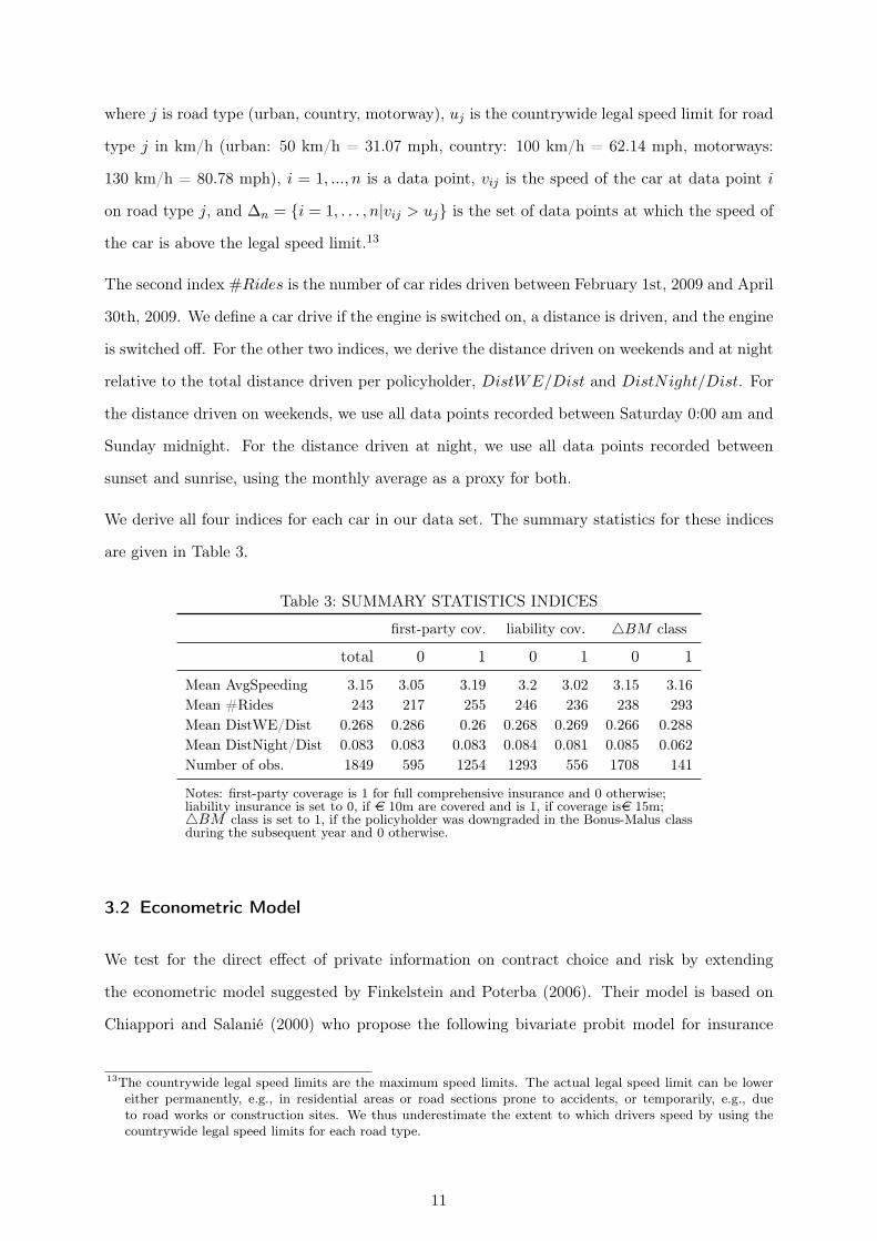
We derive all four indices for each car in our data set. The summary statistics for these indices
are given in Table 3.
Table 3: SUMMARY STATISTICS INDICES
first-party cov. liability cov. 4BM class
total 0 1 0 1 0 1
Mean AvgSpeeding 3.15 3.05 3.19 3.2 3.02 3.15 3.16Mean #Rides 243 217 255 246 236 238 293Mean DistWE/Dist 0.268 0.286 0.26 0.268 0.269 0.266 0.288Mean DistNight/Dist 0.083 0.083 0.083 0.084 0.081 0.085 0.062Number of obs. 1849 595 1254 1293 556 1708 141
Notes: first-party coverage is 1 for full comprehensive insurance and 0 otherwise;liability insurance is set to 0, if e 10m are covered and is 1, if coverage ise 15m;4BM class is set to 1, if the policyholder was downgraded in the Bonus-Malus classduring the subsequent year and 0 otherwise.
3.2 Econometric Model
We test for the direct effect of private information on contract choice and risk by extending
the econometric model suggested by Finkelstein and Poterba (2006). Their model is based on
Chiappori and Salanié (2000) who propose the following bivariate probit model for insurance
13The countrywide legal speed limits are the maximum speed limits. The actual legal speed limit can be lowereither permanently, e.g., in residential areas or road sections prone to accidents, or temporarily, e.g., dueto road works or construction sites. We thus underestimate the extent to which drivers speed by using thecountrywide legal speed limits for each road type.
11

coverage and risk
Coverage = 1(Xβ + ε1 > 0) (2)
Risk = 1(Xγ + ε2 > 0) (3)
where X is the vector of all risk classifying variables used by the insurance company. They test
the null hypothesis that the correlation ρ of the error terms ε1 and ε2 is zero and interpret reject-
ing the null hypothesis as an indication for the existence of private information. A statistically
significant, positive correlation coefficient is consistent with the classical models of adverse selec-
tion and moral hazard with asymmetric information about one parameter of the loss distribution
(Arrow, 1963; Pauly, 1974; Rothschild and Stiglitz, 1976; Harris and Raviv, 1978; Holmstrom,
1979; Shavell, 1979). Chiappori et al. (2006) show that this prediction can be extended to
general settings, including, for example, heterogeneous preferences and multidimensional hidden
information linked with hidden action. However, they point out that the prediction about the
positive relation between the level of insurance coverage and risk might no longer hold if the
degree of risk aversion is private information.
Finkelstein and Poterba (2006) propose the following extension of Chiappori and Salanié (2000)
Coverage = 1(Xβ1 + Y β2 + ε1 > 0) (4)
Risk = 1(Xγ1 + Y γ2 + ε2 > 0) (5)
where Y includes information which is observable but not used by the insurance company. Under
the null hypothesis that there is no private information contained in Y that is relevant for
contract choice and risk, we have β2 = 0 and γ2 = 0. The benefit of this model extension is that
the rejection of the null hypothesis directly provides evidence of relevant private information
independent of the type of asymmetric information. This model is appropriate in our context
in which the information Y is not observed by the insurance company but accessible to the
econometrician.
Unlike in Chiappori and Salanié (2000) and Finkelstein and Poterba (2006), policyholders in
our data set simultaneously choose the level of coverage along two dimensions, first-party and
third-party liability coverage. To take into account potential interaction between these two
choices, we apply a trivariate probit model. This model consists of three probit regressions
12

based on the Geweke-Hajivassiliou-Keane (GHK) smooth recursive simulator. Interpretation
of the results of this trivariate probit model is analogous to the interpretation of the bivariate
probit model. We define the dependent variables of the three probits as follows. For liability
coverage, we set CovLiab = 1 if the upper limit is e 15m and CovLiab = 0 if the upper limit
is e 10m. For first-party coverage, we set CovFP = 1 if the contract covers at-fault losses (full
comprehensive insurance) and CovFP = 0 otherwise. The dependent variable 4BM is set to 1
if the policyholder was downgraded in his Bonus-Malus class within the subsequent year and is
set to 0 otherwise.
X is the set of variables which the insurance company observes and uses for the pricing of the
contract (see Section 2.2). In addition, we also include the aggregate distance driven by the
policyholder since this is the part of the telematic data which the insurance company observes
and uses for setting the premium.
Y is the set of the four indices AvgSpeeding, #Rides, DistWE/Dist, and DistNight/Dist
that characterize driving behavior and are constructed from the telematic data set (see Section
3.1). This information is not observable by the insurance company. We thus apply the following
trivariate probit model
CovLiab = 1(Xβ1 + Y β2 + ε1 > 0) (6)
CovFP = 1(Xγ1 + Y γ2 + ε2 > 0) (7)
4BM = 1(Xδ1 + Y δ2 + ε3 > 0) (8)
with
Y = (AvgSpeeding,#Rides,DistWE/Dist,DistNight/Dist)
and test the null hypothesis that there is no private information contained in Y that is relevant
for contract choice and risk, i.e. we test for β2 = 0, γ2 = 0 and/or δ2 = 0.
We then compare the direct evidence about the relevance of private information with the results
obtained from the residual correlation test. In particular, we apply the model of Chiappori
and Salanié (2000) by testing for the sign of the correlation coefficients ρLiab,FP , ρLiab,4BM and
ρFP,4BM of each pair of residual error terms ε1, ε2 and ε3 both excluding and including the
set of variables Y = (AvgSpeeding, #Rides, DistWE/Dist, DistNight/Dist). Comparing the
results allows us to assess whether the conclusions that would have been drawn from the results
13

of the residual correlation test are consistent with the direct evidence. Moreover, any differences
in the results indicate additional hidden information.
4 Results and Discussion
Table 4 reports the results of the trivariate probit model, equations (6), (7), and (8).
Table 4: COEFFICIENTS OF TRIVARIATE PROBIT MODEL
CovLiab CovFP 4BM
AvgSpeeding -0.0111* 0.003 0.0026(0.0059) (0.0069) (0.0031)
#Rides -0.0002* 0.0003** 0.0002***(0.0001) (0.0001) (0.0001)
DistWE/Dist 0.0307 -0.1335 0.0934*(0.0951) (0.1119) (0.0495)
DistNight/Dist 0.1295 0.3345** -0.0463(0.1365) (0.1673) (0.0802)
kW 0.0015** -0.0005 0.0003(0.0008) (0.0009) (0.0005)
year of construction 0.0116*** 0.1003*** -0.0073***(0.0031) (0.0049) (0.0014)
value of car in e 1.41e-06 -1.04e-06 -2.75e-07(2.23e-06) (2.69e-06) (1.34e-06)
urban -0.0509** 0.0733** 0.0231**(0.0224) (0.0266) (0.0126)
male -0.0053 0.178 -0.0016(0.0236) (0.0281) (0.0123)
Bonus-Malus class -0.0342 -0.3012*** 0.043*(0.0766) (0.0884) (0.0384)
age of policyholder 0.0014* -0.0003 0.0005(0.0008) (0.001) (0.0004)
total distance driven -2.23e-08 7.49e-08*** 1.82e-08(2.08e-08) (2.67e-08) (1.08e-08)
Pseudo-R2 0.0160 0.3532 0.0508
N 1849 1849 1849
Notes: Reported coefficients are marginal effects;significance levels are labeled ***, ** and * at 1%, 5% and 10%, respectively;heteroscedastic robust standard errors are stated in parentheses.
The coefficients of the four driving indicesAvgSpeeding, #Rides,DistWE/Dist andDistNight/Dist
are reported in the first four rows for each of the three probit regressions. In the remaining rows,
we report the coefficients of the insurance company’s risk classifying variables, the Pseudo-R2,
and the number of observations. The first column reports the coefficients of the liability coverage
14

equation (6), the second column of the first-party coverage equation (7), and the third column of
the downgrade in the Bonus-Malus class equation (8). For interpreting the coefficients we only
report marginal effects. Both signs and statistical significances of coefficients are identical when
estimating the trivariate probit model simultaneously. In our following discussion we focus on
the effects of private information contained in the four driving indices.
The results in the third column show that the number of car rides is a highly statistically
significant risk factor, controlling for the distance driven. An additional car ride in the 3 month
observation period is related to a 0.02% increase in the probability of a subsequent downgrade in
the Bonus-Malus class. To illustrate the economic significance of this effect, we derive predicted
probabilities of a subsequent downgrade in the Bonus-Malus class for different numbers of car
rides. We take the estimated coefficients of our trivariate probit model and set all variables to
the mean of their empirical distribution. We then vary the number of car rides and derive the
associated probabilities of a subsequent downgrade in the Bonus-Malus class from equation (8).
Table 5 reports the predicted probabilities for the lower quartile, the mean, and the upper
quartile of the empirical distribution of the number of car rides per day. We also report the
predicted probabilities for two car rides per day, e.g. driving to work, and four car rides a day,
e.g. driving to work and separately to a supermarket. The third column shows the predicted
probabilities when adjusting the total distance driven for the average distance driven per car
ride. The differences in the predicted probabilities can be interpreted as arising from additional
car rides. The fourth column shows the predicted probabilities when keeping the total distance
driven at the mean. These differences can be related to breaks of car rides, e.g. stopping at
the supermarket on the way home from work. The differences in the predicted probabilities
are economically significant. For example, when adjusting for the average distance driven per
car ride, undertaking four as opposed to two car rides per day almost doubles the predicted
probability from 5.58% to 10.44%. But even when keeping the total distance driven at the mean,
the increase of the predicted probability from 5.95% to 9.48% is economically significant.
A possible explanation for this risk factor is that the start and the end of a car ride are particularly
exposed to accident risk since the driver has to fulfill multiple tasks such as pulling out the car
into the passing traffic, switching on the radio, adjusting the driving mirrors and seat, or parking
the car which involves slowing down, potentially looking for a parking spot, and reversing into
it. Towards the end of the drive, the driver’s mind might also be already distracted by the actual
15

Table 5: IMPACT OF #RIDES ON ∆BM
# car rides / day quantile predicted probability of ∆BM
adj. for distance driven / car ride mean total distance driven
1.22 25% 4.27% 4.90%2 42.5% 5.58% 5.95%
2.73 50% 7.09% 7.09%3.78 75% 9.78% 9.02%4 78.3% 10.44% 9.48%
purpose of the drive, e.g., a meeting, shopping, or outdoor activity. These simultaneous tasks at
the beginning and at the end of a drive might demand much more attention from the driver and
are thus more prone to accidents than the task of driving the car in the traffic.
The third column of Table 4 also shows that the relative distance driven on weekends is a
statistically significant risk factor.This result might give empirical support to the phenomenon
of Sunday drivers who use their cars relatively more during leisure time. Last, we note that
speeding is not significantly related to a downgrade in the Bonus-Malus class. This could arise
from the fact that we underestimate speeding by applying countrywide legal speed limits per
road type. In particular, we might underestimate the effect of speeding at street areas which are
prone to accident since speed limits in these areas are likely to be below the countrywide speed
limits.
We now discuss the relation between the four driving indices and contract choice, as reported in
the first and second column of Table 4. The results in the first column show that both average
speeding and the number of car rides are negatively related to the level of liability coverage. More
precisely, speeding on average one km/h (0.62 mph) more above legal speed limits is related to
a 1.11% decrease in the probability of choosing the high liability coverage option. Furthermore,
undertaking one additional car ride in the 3 month observation period is related to a 0.02%
decrease in the probability of choosing the high liability coverage option.
These results in combination with the result that the number of car rides is a significant risk factor
are opposite to the predictions of adverse selection and moral hazard. They could be explained
by selection based on heterogeneous, hidden degrees of risk aversion linked with hidden action
(de Meza and Webb, 2001) or overconfidence. Policyholders who are more risk-averse or less
overconfident purchase a higher level of liability coverage, speed on average less, undertake fewer
16

car rides, and are less likely to be downgraded in the Bonus-Malus class.14
In contrast, the results on first-party insurance coverage as shown in the second column are
consistent with the predictions of adverse selection and moral hazard. The number of car rides
is positively related to the level of first-party coverage. Policyholders who undertake more car
rides are more likely to purchase full comprehensive insurance coverage and more likely to be
downgraded in their Bonus-Malus class. Specifically, undertaking an additional car ride in the
3 month observation period is associated to a 0.03% increase in the probability of choosing full
comprehensive insurance coverage. Last, the relative distance driven at night is positively related
to the level of first-party coverage.
In summary, the results of the trivariate probit model show that there exists private information
contained in the four driving indices that is relevant for contract choice and risk as measured by a
subsequent downgrade in the Bonus-Malus class. Furthermore, the effects related to third-party
liability coverage are opposite to the effects related to first-party coverage. The results suggest a
negative association between the level of liability coverage and risk, while they suggest a positive
association between the level of first-party coverage and risk. These opposite correlation signs
could result from an overlay of risk-based and preference-based selection effects. The risk-based
selection originates from private information on risk characteristics which overlays the selection
based on preferences such as risk aversion. Since the potential severity of liability claims is much
higher than the one of first-party claims, the preference-based selection might have a relatively
stronger effect on liability coverage than it has on first-party coverage. Differences in the degrees
of risk aversion might be a much more important factor when facing claims in millions of e than
when facing a loss that is restricted by the value of the car. This would explain the opposite
effects on liability and on first-party coverage.15
In Table 6, we report the correlation coefficients ρLiab,FP , ρLiab,4BM , and ρFP,4BM of each pair14Our results show that the level of liability coverage is positively related to the age of the policyholder. There
is empirical evidence that individuals become less risk averse when they get older (e.g., Morin and Suarez,1983; Bucciol and Miniaci, 2011). This supports our conjecture that risk aversion effects the choice of liabilitycoverage.
15While it is true that individuals who are more risk-averse value insurance coverage more, the effect of riskaversion on the value of risk control is ambiguous (see Ehrlich and Becker, 1972; Dionne and Eeckhoudt,1985; Jullien et al., 1999). Moreover, if insurance coverage and risk control are substitutes, then a higherlevel of insurance coverage might reduce the willingness to invest in risk control. Depending on the setting,more risk-averse individuals might as well purchase more insurance coverage but invest less in risk controland thereby be of higher risk. Jullien et al. (2007) develop a principal-agent model with hidden degree ofrisk aversion and show that, depending on the parameters, the correlation between insurance coverage andrisk can be positive, negative, or zero. Cohen and Einav (2007) present a structural model which accountsfor unobserved heterogeneity in both risk and risk aversion. By using a large data set of an Israeli insurancecompany they find a strong positive correlation between unobserved risk aversion and unobserved risk whichstrengthens the positive correlation property.
17

of residual error terms in the trivariate probit model, equations (6), (7), and (8).
Table 6: CORRELATIONS OF RESIDUAL ERROR TERMS
without private information with private information
ρLiab,FP 0.113** 0.128***(0.0106) (0.0041)
ρLiab,4BM 0.061* 0.06*(0.0822) (0.0944)
ρFP,4BM -0.015 0.000(0.7311) (0.9967)
N 1849 1849
Notes: significance levels are labeled ***, ** and * at 1%, 5% and 10%, respectively;heteroscedastic robust standard errors are stated in parentheses.
We first test for the positive correlation property between insurance coverage and risk as if we did
not have access to the additional private information contained in Y . The first column reports the
correlation coefficients when excluding the four driving indices from the trivariate probit model.
This model is thus a trivariate version of the model of Chiappori and Salanié (2000), equations
(2) and (3). The results show that we fail to reject the null hypothesis of zero correlation
between first-party coverage and a downgrade in the Bonus-Malus class, ρFP,4BM = 0, which is
consistent with the results of most empirical studies in automobile insurance, see e.g. Chiappori
and Salanié (2000) and Dionne et al. (2001). As discussed in Chiappori et al. (2006) and
Finkelstein and Poterba (2006), we cannot draw unambiguous conclusions from failing to reject
the null hypothesis about the existence and relevance of asymmetric information. And this is
exactly confirmed by our direct evidence. Although we fail to reject the null hypothesis of zero
residual correlation between first-party coverage and a downgrade in the Bonus-Malus class, we
do find that private information, in particular the number of car rides, is relevant for the level
of first-party insurance coverage and for a downgrade in the Bonus-Malus class (see Table 4).
A similar conclusion must be drawn about interpreting the statistically significant positive corre-
lation of the residual error terms between liability coverage and a downgrade in the Bonus-Malus
class, ρLiab,4BM . The positive sign of the correlation coefficient is new to the literature which
has focused on first-party coverage. This could be interpreted as arising from adverse selection
and/or incentive effects. However, the negative relation of both average speeding and number of
car rides to the level of liability insurance coverage (see Table 4) suggest at least an additional
preference-based selection effect which is opposite to the one of adverse selection. The positive
18

correlation coefficient in conjunction with the results on average speeding and the number of car
rides is thus another indication of overlaying risk-based and preference-based selection effects.
Last, the correlation between the residual error terms of the liability and first-party coverage
equations ρLiab,FP is highly statistically significant and positive. This is consistent with some
private information, such as risk aversion, which explains why policyholders who choose full
comprehensive coverage also choose the high liability coverage option.
The second column in Table 6 reports the correlation coefficients between the residual error
terms when including the four driving indices in the trivariate probit model. The results do
not change. The correlation coefficient ρFP,4BM between the error terms of first-party coverage
and risk remains to be not statistically different from zero. Similarly, the correlation coefficients
ρLiab,FP and ρLiab,4BM between the error terms of liability and first-party coverage and between
liability coverage and risk remain statistically significant and positive.
5 Robustness
5.1 Selection Bias
The pay-as-you-drive insurance contract is offered for choice. Hence there might be a selection
bias if the characteristics of policyholders who choose the pay-as-you-drive insurance contract
are correlated with the three dependent variables. To control for the potential selection bias, we
employ a Heckman correction method based on an additional data set of randomly selected 2000
cars which are insured under the traditional insurance contract. The policyholders contained
in this data set thus decided not to switch to the pay-as-you-drive contract. Data cleaning
(excluding cars with less than 4 kW = 5.4 HP) leaves us with 1987 traditional insurance contracts.
Table 7 provides the summary insurance statistics under the traditional insurance contract.
In our context, we have a probit selection equation and a trivariate probit outcome equation.
Since we are not aware of a sample selection model in connection with a trivariate probit re-
gression we run three separate bivariate probit models with sample selection. In each model, we
simultaneously run a probit model in the selection equation and a probit model in the outcome
equation. While the selection equation is identical in all three models, the outcome equation
varies according to the three variables of interest: the level of liability coverage, the level of
first-party coverage, and the subsequent downgrade in the Bonus-Malus class.
19

Table 7: SUMMARY STATISTICS TRADITIONAL INSURANCE DATA
Mean
total none/compr. full compr. liab. 10m liab. 15m
car’s characteristics:years since construction 5.32 7.18 0.94 5.53 4.83kW 75.83 74.41 79.17 75.49 76.62(HP)(0.0027) (101.69) (99.79) (106.17) (101.23) (102.75)value of car in e 22,768 22,615 23,127 22,588 23,188
policyholder’s characteristics:age in years 54.65 54.82 54.25 54.57 54.83male 0.67 0.70 0.63 0.68 0.67urban 0.21 0.19 0.25 0.20 0.21BM (Bonus-Malus class) 0.46 0.46 0.45 0.46 0.45
number of obs. 1987 1394 593 1392 595
Notes: Column 2 “none/compr.” includes contracts with no first-party insurance coverage or comprehensivecoverage; Column 3 “full compr.” includes contracts with comprehensive coverage and at-fault collision;Bonus-Malus class gives the scaling factor for the base premium of liability coverage.
The selection equation
Selection = 1(Xγ1 + ε1 > 0)
is based on both samples of policyholders, the randomly selected sample of those who chose not
to sign up and the sample of those who signed up for the pay-as-you-drive insurance contract.
Selection is a binary variable, equal to 1 if the policyholder chose the pay-as-you-drive insurance
contract and equal to 0 if the policyholder chose the traditional insurance contract. X consists
of all the variables used by the insurance company for pricing the traditional insurance contract.
The outcome equation in each of the three regressions is given by
Outcome = 1(Xβ1 + Y β2 + ε2 > 0) (9)
where the variable Outcome in the three bivariate probit models with sample selection is either
CovLiab for liability coverage, or CovFP for first-party coverage, or 4BM for a subsequent
downgrade in the Bonus-Malus class.
We use the gender variable male as an instrumental variable since it indicates the gender of the
person that purchased the insurance contract. This person is thus likely to be the one who decides
whether to switch to the pay-as-you-drive insurance contract or not. However, this person is not
necessarily the person who mainly drives the car since the insurance contract is related to the
car and not to the specific driver. In fact, any person who drives the car with the approval of
20

the policyholder is insured under the contract.
Table 8 reports the results of the selection equation. It shows that all the variables are highly
significant for the selection of the type of insurance contract. The pay-as-you-drive insurance
contract is more likely to be chosen by younger and female individuals who live in urban areas
and are in a higher Bonus-Malus class. Moreover, they own newer, more valuable cars with more
engine power.
Table 8: RESULTS OF SELECTION EQUATION
Coefficients
kW 0.0019***(0.0006)
year of construction 0.0195***(0.0018)
value of car in e 3.86e-06**(1.62e-06)
urban 0.2692***(0.0171)
male -0.0666***(0.0185)
Bonus-Malus class 1.6062***(0.1061)
age of policyholder -0.0066***(0.0006)
Pseudo-R2 0.1733
N 3985
Notes: Reported coefficients are marginal effects;significance levels are labeled ***, ** and * at1%, 5% and 10%, respectively; heteroscedasticrobust standard errors are stated in parentheses.
Table 9 reports the coefficients of the outcome equation and shows that our results on the
relevance and effects of private information contained in the four driving indices AvgSpeeding,
#Rides, %DistWE and %DistNight are robust when controlling for a selection-bias. The
only exception is that the relation between the relative distance driven during weekends and a
subsequent downgrade in the Bonus-Malus class loses its significance.
We conclude that while policyholder’s and car’s characteristics are relevant for the decision to
sign up for the pay-as-you-drive insurance contract this selection does not affect the within-group
correlations between driving behavior and the level of liability coverage, the level of first-party
coverage, and a subsequent downgrade in the Bonus-Malus class.
21
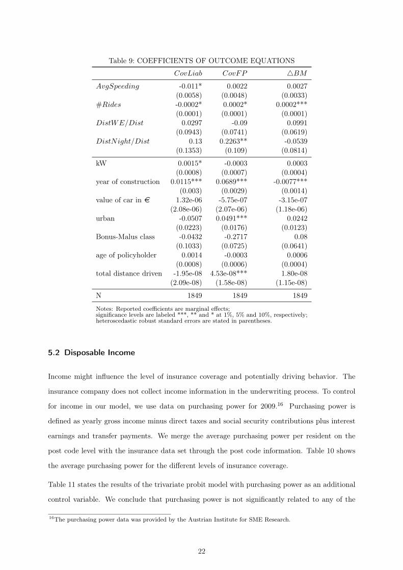
Table 9: COEFFICIENTS OF OUTCOME EQUATIONS
CovLiab CovFP 4BM
AvgSpeeding -0.011* 0.0022 0.0027(0.0058) (0.0048) (0.0033)
#Rides -0.0002* 0.0002* 0.0002***(0.0001) (0.0001) (0.0001)
DistWE/Dist 0.0297 -0.09 0.0991(0.0943) (0.0741) (0.0619)
DistNight/Dist 0.13 0.2263** -0.0539(0.1353) (0.109) (0.0814)
kW 0.0015* -0.0003 0.0003(0.0008) (0.0007) (0.0004)
year of construction 0.0115*** 0.0689*** -0.0077***(0.003) (0.0029) (0.0014)
value of car in e 1.32e-06 -5.75e-07 -3.15e-07(2.08e-06) (2.07e-06) (1.18e-06)
urban -0.0507 0.0491*** 0.0242(0.0223) (0.0176) (0.0123)
Bonus-Malus class -0.0432 -0.2717 0.08(0.1033) (0.0725) (0.0641)
age of policyholder 0.0014 -0.0003 0.0006(0.0008) (0.0006) (0.0004)
total distance driven -1.95e-08 4.53e-08*** 1.80e-08(2.09e-08) (1.58e-08) (1.15e-08)
N 1849 1849 1849
Notes: Reported coefficients are marginal effects;significance levels are labeled ***, ** and * at 1%, 5% and 10%, respectively;heteroscedastic robust standard errors are stated in parentheses.
5.2 Disposable Income
Income might influence the level of insurance coverage and potentially driving behavior. The
insurance company does not collect income information in the underwriting process. To control
for income in our model, we use data on purchasing power for 2009.16 Purchasing power is
defined as yearly gross income minus direct taxes and social security contributions plus interest
earnings and transfer payments. We merge the average purchasing power per resident on the
post code level with the insurance data set through the post code information. Table 10 shows
the average purchasing power for the different levels of insurance coverage.
Table 11 states the results of the trivariate probit model with purchasing power as an additional
control variable. We conclude that purchasing power is not significantly related to any of the
16The purchasing power data was provided by the Austrian Institute for SME Research.
22

Table 10: SUMMARY STATISTICS PURCHASING POWER
Mean
total none/compr. full compr. liab. 10m liab. 15m
purchasing power in e 17,572 17,369 17,668 17,597 17,513
Notes: Column 2 “none/compr.” includes contracts with no first-party insurance coverageor comprehensive coverage; Column 3 “full compr.” includes contracts with comprehensive coverageand at-fault collision; Bonus-Malus class gives the scaling factor for the premium of liability coverage.
three dependent variables. More importantly, our results are robust to including purchasing
power as an additional variable.
Table 11: COEFFICIENTS OF TRIVARIATE PROBIT MODEL
CovLiab CovFP 4BM
AvgSpeeding -0.0116* 0.0037 0.0024(0.0059) (0.0072) (0.0031)
#Rides -0.0002* 0.0003** 0.0002***(0.0001) (0.0001) (0.0001)
%DistWE 0.0300 -0.1335 0.0935*(0.0954) (0.1119) (0.0582)
%DistNight 0.1295 0.3345** -0.0459(0.1365) (0.1673) (0.0770)
kW 0.0015* -0.0005 0.0003(0.0008) (0.0011) (0.0004)
years since construction -0.0117*** -0.1002*** 0.0073***(0.0030) (0.0070) (0.0013)
value of car in e 1.50e-06 -1.24e-06 -2.42e-07(2.12e-06) (3.14e-06) (1.12e-06)
urban -0.04778* 0.0681** 0.0244**(0.0228) (0.0269) (0.0127)
male -0.0067 0.199 -0.002(0.0232) (0.0271) (0.0126)
Bonus-Malus class -0.0322 -0.3050*** 0.044*(0.0833) (0.0884) (0.0377)
age of policyholder 0.0014* -0.0004 0.0005(0.0008) (0.0009) (0.0004)
total distance driven -2.22e-08 7.33e-08*** 1.83e-08(2.24e-08) (2.45e-08) (1.12e-08)
purchasing power in e -3.17e-06 5.30e-06 -1.32e-06(4.03e-06) (5.23e-06) (2.00e-06)
Pseudo-R2 0.0162 0.3537 0.0512
N 1849 1849 1849
Notes: Reported coefficients are marginal effects;significance levels are labeled ***, ** and * at 1%, 5% and 10% respectively;heteroscedastic robust standard errors are stated in parentheses.
23

Table 12 shows the results for the residual correlation when including purchasing power in the
trivariate probit model. Again, our results do not change.
Table 12: CORRELATIONS OF RESIDUAL ERROR TERMS
without private information with private information
ρLiab,FP 0.125*** 0.133***(0.0044) (0.003)
ρLiab,4BM 0.06* 0.06*(0.0728) (0.0913)
ρFP,4BM 0.006 0.007(0.8822) (0.8691)
N 1849 1849
Notes: significance levels are labeled ***, ** and * at 1%, 5%and 10% respectively; p values are stated in parentheses.
6 Conclusions
We capitalize on having access to detailed data on driving behavior of policyholders in automobile
insurance which is inaccessible to the insurance company. By connecting this data to insurance
data, we provide direct evidence that driving behavior is relevant for contract choice in first-
party and third-party liability insurance as well as for risk. Whereas number of car rides and
average speeding above legal speed limits is negatively related to the level of liability coverage, the
number of car rides and the relative distance driven at night are positively related to the level of
first-party insurance coverage. Moreover, the number of car rides and the relative distance driven
on weekends are significant risk factors. These results pulled together suggest the coexistence
and interaction of risk-based and preference-based selection effects.
We then test for the residual correlation between insurance coverage and risk which would be
the standard test for asymmetric information if we did not have access to the data on driving
behavior. The results emphasize that the residual correlation test can be misleading when
interpreted in the context of asymmetric information. We fail to reject the hypothesis of zero
residual correlation between first-party coverage and risk although the number of car rides is
positively related to both first-party insurance coverage and risk. Similarly, we find a significant
positive residual correlation between liability coverage and risk although the number of car rides
is negatively related to liability coverage but positively related to risk.
24

References
[1] Arrow, K.J., 1963, Uncertainty and the Welfare Economics of Medical Care, American
Economic Review 53(5), 941-973
[2] Bucciol, A., and R. Miniaci, 2011, Household Portfolios and Implicit Risk Preference, Review
of Economics and Statistics 93(4), 1235-1250
[3] Cawley, J., and T. Philipson, 1999, An Empirical Examination of Information Barriers to
Trade in Insurance, American Economic Review 89(4), 827-846
[4] Chiappori, P.-A., B. Jullien, B. Salanié, and F. Salanié, 2006, Asymmetric Information in
Insurance: General Testable Implications, RAND Journal of Economics 37(4), 783-798
[5] Chiappori, P.-A., and B. Salanié, 2000, Testing for Asymmetric Information in Insurance
Markets, Journal of Political Economy 108(1), 56-78
[6] Cohen, A., 2005, Asymmetric Information and Learning in the Automobile Insurance Mar-
ket, Review of Economics and Statistics 87(2), 197-207
[7] Cohen, A., and L. Einav, 2007, Estimating Risk Preferences from Deductible Choice, Amer-
ican Economic Review 97(3), 745-788
[8] Cohen, A., and P. Siegelmann, 2010, Testing for Adverse Selection in Insurance Markets,
Journal of Risk and Insurance 77(1), 39-84
[9] Cutler, D.M., and S.J. Reber, 1998, Paying for Health Insurance: The Trade-Off Between
Competition and Adverse Selection, Quarterly Journal of Economics 113(2), 433-466
[10] Cutler, D.M., and R.J. Zeckhauser, 1998, Adverse Selection in Health Insurance, Forum
for Health Economics and Policy : Vol. 1: (Frontiers in Health Policy Research), Article 2.
http://www.bepress.com/fhep/1/2
[11] de Meza, D., and D.C. Webb, 2001, Advantageous Selection in Insurance Markets, RAND
Journal of Economics 32(2), 249-262
[12] Dionne, G., and L. Eeckhoudt, 1985, Self-Insurance, Self-Protection and Increased Risk
Aversion, Economics Letters 17(1-2), 39-42
[13] Dionne, G., C. Gouriéroux, and C. Vanasse, 2001, Testing for Evidence of Adverse Selection
in the Automobile Insurance Market: A Comment, Journal of Political Economy 109(2),
444-453
25

[14] Edlin, A.S., 2003, Per-Mile Premiums for Auto Insurance, in Economics for an Imperfect
World: Essays In Honor of Joseph Stiglitz, Ed. Richard Arnott, Bruce Greenwald, Ravi
Kanbur, Barry Nalebuff, MIT Press, 53-82
[15] Edlin, A.S., and P. Karaca-Mandic, 2006, The Accident Externality from Driving, Journal
of Political Economy 114(5), 931-955
[16] Ehrlich, I, and G. Becker, 1972, Market Insurance, Self-Insurance, and Self-Protection,
Journal of Political Economy 80(4), 623-648
[17] Fang, H., M.P. Keane, and D. Silverman, 2008, Sources of Advantageous Selection: Evidence
From the Medigap Insurance Market, Journal of Political Economy 116(2), 303-350
[18] Finkelstein, A., and K. McGarry, 2006, Multiple Dimensions of Private Information: Ev-
idence From the Long-Term Care Insurance Market, American Economic Review 96(4),
938-958
[19] Finkelstein, A., and J. Poterba, 2004, Adverse Selection in Insurance Markets: Policyholder
Evidence From the U.K. Annuity Market, Journal of Political Economy 112(1), 183-208
[20] Finkelstein, A., and J. Poterba, 2006, Testing for Adverse Selection with Unused Observ-
ables, NBER Working Paper No. 12112
[21] Gan, L., M.D. Hurd, and D.L. McFadden, 2005, Individual Subjective Survival Curves, in
D. Wise (ed.), Analysis in the Economics of Aging, Chicago: University of Chicago Press,
377-411
[22] Hurd, M.D., 1999, Anchoring and Acquiescence Bias in Measuring Assets in Household
Surveys, Journal of Risk and Uncertainty 19(1-3), 111-136
[23] Hurd, M.D., D.L. McFadden, H. Chand, L. Gan, A., and M. Roberts, 1998, Consumption
and Saving Balances of the Elderly: Experimental Evidence on Survey Response Bias, in D.
Wise (ed.), Topics in the Economics of Aging, Chicago: University of Chicago Press, 353-87
[24] Harris, M., and A. Raviv, 1978, Some Results on Incentive Contracts With Applications to
Education and Employment, Health Insurance, and Law Enforcement, American Economic
Review 68(1), 20-30
[25] Holmstrom, B., 1979, Moral Hazard and Observability, Bell Journal of Economics 10(1),
74-91
26

[26] Jullien, B., S. Salanié, and F. Salanié, 1999, Should More Risk-Averse Agents Exert More
Effort?, The Geneva Papers on Risk and Insurance Theory 24(1), 19-28
[27] Jullien, B., S. Salanié, and F. Salanié, 2007, Screening Risk-Averse Agents Under Moral
Hazard: Single-Crossing and the CARA Case, Economic Theory 30(1), 151-169
[28] Koufopoulos, K., 2007, On the Positive Correlation Property in Competitive Insurance
Markets, Journal of Mathematical Economics 43(5), 597-605
[29] McCarthy, D., and O.S. Mitchell, 2010, International Adverse Selection in Life Insurance
and Annuities, in S. Tuljapurkar, N. Ogawa, and A.H. Gauthier (eds.), Ageing in Advanced
Industrial States: Riding the Age Waves, Vol. 3, Springer, 119-135
[30] Morin, R., and A. Suarez, 1983, Risk Aversion Revisited, Journal of Finance 38(4), 1201-
1216
[31] Pauly, M.V., 1974, Overinsurance and Public Provision of Insurance: The Role of Moral
Hazard and Adverse Selection, Quarterly Journal of Economics 88(1), 44-62
[32] Puelz, R., and A. Snow, 1994, Evidence on Adverse Selection: Equilibrium Signaling and
Cross-Subsidization in the Insurance Market, Journal of Political Economy 102(2), 236-257
[33] Rothschild, M., and J. Stiglitz, 1976, Equilibrium in Competitive Insurance Markets: An
Essay on the Economics of Imperfect Information, Quarterly Journal of Economics 90(4),
629-649
[34] Saito, K., 2006, Testing for Asymmetric Information in the Automobile Insurance Market
Under Rate Regulation, Journal of Risk and Insurance 73(2), 335-356
[35] Shavell, S., 1979, On Moral Hazard and Insurance, Quarterly Journal of Economics 93(4),
541-562
[36] Vickrey, W., 1968, Automobile Accidents, Tort law, Externalities and Insurance: An
Economist’s Critique, Law and Contemporary Problems 33(3), 464-487
27