astronomy and spectral analysis of the magnetic ﬁeld

Astron. Astrophys. 351, 385–392 (1999) ASTRONOMYAND

ASTROPHYSICS

Spectral analysis of the magnetic field inside particle propagationchannels detected by Ulysses

A. Buttighoffer 1,2,?, L.J. Lanzerotti 2, D.J. Thomson2, C.G. Maclennan2, and R.J. Forsyth4

1 Space Sciences Lab., University of California, Berkeley, CA 94720, USA2 Lucent Technologies, Bell Laboratories, Murray Hill, NJ 07974, USA3 Space and Atmospheric Physics, The Blackett Laboratory, Imperial College, London SW7 2BZ, UK

Received 19 August 1998 / Accepted 27 August 1999

Abstract. Prior studies have identified particle propagationchannels in the interplanetary medium where nearly scatter–free propagation occurs. These channels have been identified toexist as far away from the Sun as∼4 AU. We report here a studythat has examined, using spacecraft–based instrumentation, thenature of the fluctuations of the interplanetary magnetic fieldsinside two such propagation channels as well as in the regionsoutside the channels. We show that the power spectral fluctua-tions of the total magnitude of the magnetic field in the entirechannel duration encountered are the order of a factor of 10lower inside the channels than outside. Somewhat surprisingly,in the 1–40 mHz frequency range, we find little change in theslope of the power law spectra from outside to inside the chan-nels. These results provide evidence that the dominant controlon the particle pitch angle diffusion coefficients in the channelsis the level of power available for particle scattering, and notchanges in the shape of the spectra themselves. We have exam-ined the power spectra of each component of the magnetic fieldand determined that the loss of spectral power is due to a reduc-tion of compressible fluctuations, the solenoidal components ofthe spectra remaining similar inside and outside the channels.

Key words: Sun: corona – Sun: particle emission – Sun: radioradiation – inteplanetary medium

1. Introduction

The problem of solar particle propagation in the interplanetarymedium is an old one. It has long been studied both theoreti-cally and observationally by use of in–situ measurements. Theimportance of the interplanetary magnetic field, and especiallyits fluctuations (characterized by variations in the power spec-tra computed from time series of the field data), has been wellestablished theoretically. The “standard model”, Quasi Linear

Send offprint requests to: A. Buttighoffer([email protected])

? Present address:LPSH UMR 8645, Observatoire de Meudon, 5place Janssen, 92195 Meudon, France

Theory (QLT) with the ‘slab model’ of magnetic field fluctu-ations, for example, can be used to compute the pitch anglediffusion coefficient of the propagating particles (whose evolu-tion governs different propagation regimes) from magnetic fieldpower spectra. The interplanetary power spectrumP (f) is usu-ally characterized as a power law, with power law exponentαand the power levelP (f0) at some frequencyf0. It has beenshown by Beeck & Wibberenz (1986) that the pitch angle dif-fusion coefficient can be related to measured parameters suchas the particle pitch angle distribution to test the validity of thevarious propagation theories. See also Valdes–Galicia (1993)for a review on those theories and the different corrections thatcan be applied to QLT.

Power spectra of magnetic field fluctuations have long beenstudied in the heliosphere. A comprehensive review of thosestudies can be found in Tu & Marsch (1995). Special emphasiswas often made on Alfvenic fluctuations and the study of theradial evolution of their spectra (see for example Bavassano etal. (1982b)). Actual determinations ofα andP (f0) during timeintervals when impulsive solar particle events were observedhave been reported by Tan & Mason (1993). This study showsthat despite the predictions of the slab model, the value ofαdid not appear to have a significant difference in defining thepropagation regimes. They reported, however, thatP (f0) wassubstantially lower during time intervals when scatter-free par-ticles were observed.

On the purely observational side of the problem, it hasbeen shown that impulsive solar particle events are observedinside special plasma structures that are rooted on the solar sur-face. These were called ‘propagation channels’ by Anderson &Dougherty (1986) from measurements made near 1 AU. Morerecently, Buttighoffer et al. (1995) showed that such plasmastructures were still observed to channel particle propagationwell beyond 1 AU, and that the main characteristic of such astructure was a magnetic field with a very low variance (muchlower than the one observed outside the channel). A statisticalstudy of solar impulsive electron events observed by Ulyssesin association with radio type III bursts and Langmuir waves(Buttighoffer, 1998) established that such events were all ob-served in association with particle channels with low magneticfield variances. The channels seemed to be privileged locations

386 A. Buttighoffer et al.: Magnetic field spectra inside propagation channels

for both nearly scatter-free particle propagation and Langmuirwave excitation. Such a channel is shown on Fig. 1 see alsoFig. 1 of Buttighoffer (1998). Another important aspect of thosestudies was to establish that the channels were very strongly or-ganized by the magnetic field; in particular, the fluctuationalenergy was confined to a plane perpendicular to the mean mag-netic field. No polarization of fluctuations in this plane could befound.

We report here a study of the power spectra of magneticfield fluctuations inside two propagation channels observed byUlysses. We seek a more theoretical understanding of whynearly scatter-free particle propagation, or Langmuir waves ex-citation, is favored inside the channels. We examine spectra(0.1–40 mHz) of the magnetic field magnitude, the spectra ofeach vector component, and the time variations of the valuesof α andP (f0 = 20mHz) made from power law fits in the 1to 40 mHz range. The data analyzed here have been obtainedby the Ulysses magnetic field experiment (Balogh et al., 1992).As often occurs in experimental data time series analysis, bothdata resolution changes (due here to changes in telemetry rates)and short duration data gaps (on the order of a few seconds to aminute) are occasionally present and affect the spectral analysis.In the following section of this paper we discuss the character-istics of those resolution changes and data gaps, how we havechosen to deal with them, and present a statistical analysis whichestablishes that the ‘completion method’ chosen has no signifi-cant effect on the spectral parameters obtained. Sect. 3 presentsthe results on the magnetic field spectra in the channels, andSect. 4 discusses these results and compares them to previousstudies reported near 1 AU by Tan & Mason (1993).

2. Analysis

The goal of this analysis is to determine the spectral propertiesof the magnetic field fluctuations in the channels and to comparethem with the properties of the surrounding plasma in order todetermine why nearly scatter-free propagation and/or Langmuirwave excitation might occur there. Buttighoffer et al. (1995) andButtighoffer (1998) have shown that magnetic field fluctuationsare geometrically organized (with a very clearly defined mini-mum variance direction) in the channels. Thus, a spectral anal-ysis has to be performed not only on the field magnitude, butalso on the different components in order to investigate possiblegeometric differences in the spectra.

The frequency domain of interest for electron propa-gation1 is around fgyr = qB

2πγmo= qB

2πmo

11+Ec/Eo

≈28.01 B(nT )

1+Ec/Eo(Hz). Here,fgyr is the electron gyro-frequency,

γ the Lorentz factor,Ec the electron kinetic energy,E0 =m0c

2 the mass energy at rest,q the electric charge, and Bis the local magnetic field magnitude. For the 30 to 300 keVelectrons detected by the HISCALE instrument on Ulysses

1 The channels studied here were discovered when we studied impul-sive solar electron events associated with radio Type III bursts measuredby Ulysses (Buttighoffer, 1998)

(Lanzerotti et al., 1992) in an average value of magnetic fieldof 1 nT,fgyr ranges from 18 to 26 Hz. The magnetic field reso-lution required to reach such a frequency would be of the orderof some 100 samples a second and is not accessible on Ulysses.For ions, on the contrary,fgyr ≈16 mHz and is in the frequencyrange of the spectrum obtained from our 12 s resolution data(highest limit of 40 mHz with our spectral analysis method).

At the other end of the spectrum, the lower frequency limitis determined by the length of the data set used, and this is ulti-mately limited by the length of time that the spacecraft spends ina channel. One of the possibilities is to compute spectra for thetotal length of time in the channels and compare these spectrato the same time length of data taken before and after channelcrossing. This analysis process has a major drawback: since thetime intervals in the channels are not the same it is very difficultto interpret the differences inα, P (f0) or the spectra in theirentirety. Even worse, all dynamic effects that might exist in achannel would be lost. We therefore have chosen to computespectra over a 2 hour time interval using a 2 hour sliding win-dow to produce dynamic spectra. Each spectrum is slid in timeby 12 s from the preceding spectrum. The frequency domain ofthe spectra will then be from 0.13 to 40 mHz with a frequencyresolution of 0.13 mHz.

An inspection of the different data sets used in the analysisshows that the data gaps are mostly of short duration (a fewminutes is a maximum) and do not appear very often (3–4 suchgaps in a typical 24 h data set). The spectral analyses were ac-complished using a fast Fourier transformation algorithm afterapplying a prolate window function to the data in the time do-main (Thomson, 1982). A mean value was also subtracted fromeach data set. This analysis requires a data set without gaps. Alinear interpolation procedure was used to fill the gaps and to ob-tain a new data set. We carried out a detailed statistical analysisof the way this interpolation could interfere with our analysistechnique in order to evaluate the validity and confidence in-terval on our spectral parameters. This analysis is presented inAppendix and shows that the linear interpolations used to fillthe data gaps does not introduce excessive bias.

3. Results

The two channels studied here were crossed by Ulysses onApril 20, 1991 from 12:30 UT to 18:00 UT and on Septem-ber 26, 1991 between 10:00 UT and 23:00 UT. At these timesthe spacecraft was at about 5◦ S of the ecliptic plane and at he-liocentric distances of 2.77 and 4.28 AU respectively. Minimummagnetic field variance analysis performed on data from thesedays shows that the direction of the minimum variance is verywell defined along the mean magnetic field inside the chan-nels (i.e., most of fluctuational energy>70% is dissipated inthe perpendicular plane). Note that these properties (minimumvariance along the mean magnetic field and fluctuations orthog-onal to this direction) are rather usual in the solar wind; see, forexample, Bavassano et al. (1982a) or Klein et al. (1993). They

A. Buttighoffer et al.: Magnetic field spectra inside propagation channels 387

Fig. 1. This figure presents different observations made by Ulyssesspacecraft on April 20, 1991 when a propagation channel (delimitedhere by dashed lines) was crossed. From top to bottom, a URAP/RARradio spectrogram; evolutions of plasma noise level at 5 kHz (close tothe local plasma frequency); 40 keV electron fluxes (e); total (|B|) andradial (Br) magnetic field; solar wind speed (|V |) and interplanetaryplasma electron density (Ne) are presented.

are compatible with Alfvenic turbulence2. So here the contrastbetween the inside and outside of the channels indicates that tur-bulence inside channels is not only less important in magnitudebut also different in nature: more Alfvenic than outside.

The case of September 26, 1991, is very interesting in thatthe minimum variance direction before channel entry and afterchannel exit is approximately the same as that inside the chan-nel. The minimum variance direction on this day was almostthe tangential direction (Buttighoffer et al., 1995); therefore thespectra computed directly from data in the RTN local helio-centric coordinate system correspond to those in the varianceeigen-vector base. Thus, no coordinate system transformationis needed to detect a possible counterpart to the geometrical

2 Due to the different resolution and measurement gaps between theplasma and magnetic field instruments, it is difficult to observe thecorrelation between magnetic field and plasma velocity. It is there-fore impossible to strictly prove that we have Alfven waves. Howeversince interpolated and degraded resolution (5–10 min) data plots arecompatible with Alfven modes, this hypothesis seems quite reasonable

Fig. 2.Comparison between spectra computed for September 26, 1991,before and after the channel crossing for the same duration (13 hours).Note that a median filter has been applied to the spectra at frequencieshigher than 2 mHz in order to reduce the spectral noise observed atthose frequencies.

Fig. 3. Comparison between spectra computed for April 20, 1991, be-fore and after the channel crossing for the same duration (05:30 hours).Note that a median filter has been applied to the spectra at frequencieshigher than 2 mHz in order to reduce the spectral noise observed atthose frequencies.

effects defined by the minimum variance analysis:T is the min-imal variance direction along which fluctuations are compres-sional;R andN define the maximal variance plane and containsolenoidal fluctuations.

For April 20, however, these geometrical features are notpresent. The minimum variance direction inside the channelis constant but not in the same direction as before and after


the channel crossing. This is why any simple coordinate sys-tem transformation that is designed to obtain data in the eigen-vector base is impossible for this day. We have therefore chosento compute spectra in theRTN local heliocentric coordinatesystem for this day. This coordinate system has some physicalmeaning as R is the radial direction away from the Sun and N isorthogonal to the ecliptic plane. If there are geometrical effectsassociated with different expansions of the plasma away fromthe Sun between the channel and its surrounding medium, theyshould be easier to detect using this coordinate system.

The spectral analysis study was carried out in two differentways. In the first study, a comparison is made between spectralparameters calculated from data from the entire channel dura-tion and those determined for similar data durations before andafter channel crossing. In the second, a dynamic spectral analy-sis study was made using a 2 hour sliding window over the datasets beginning a few hours before channel entry and ending afew hours after channel exit. The time increment in the slidingwindow is 12 s.

3.1. Spectra for entire channels

Figs. 2 and 3 are plots of the power spectra of magnetic fieldmagnitude and its 3 components made inside each channelfor the entire channel duration (respective durations of 13 and5.5 hours) and for the same duration interval outside the chan-nel. It is clear from these plots that the magnetic field spectralpower is much less inside the channels (about almost an orderof magnitude less at all frequencies) than outside. This resultis not surprising since channels were characterized by muchlower magnetic field variance than the surrounding plasma. Dif-ferences are more clearly visible in the spectra of the magneticfield magnitude, and for September 26, 1991, also on theT com-ponent. It appears, on the other hand, that the spectral slopes aresimilar inside and outside the channels. As pointed out in Sect. 2,a comparison between the spectra in the two intervals obtainedinside the channels is not possible since they are calculated withtotal time durations.

3.2. Dynamic spectra

Dynamic spectra made with a 2 hour sliding window allow oneto follow the evolution of the different spectral parameters in-side the channel as well as during channel entry and exits. Fig. 4presents the evolution with time ofα andP (f0 = 20 mHz)during April 20, 1991. It is obvious that bothα andP (f0 =20 mHz) have variations with time outside and inside the chan-nel (which occurs between the two vertical lines in each panel).P (f0 = 20 mHz) appears to be less variable inside the channelthan outside when determined from these 2 hour spectra. How-ever, while there is some indication that the power is less insidethe channel than in the intervals prior to channel crossing, theeffect we see on these 2 hour spectra is not as large as that seenon spectra made inside the entire channel (Figs. 2 and 3). Onthe contrary, there are no significant changes in the values andvariations ofα that characterize a channel crossing. This is con-

Fig. 4. Plots ofα andP (f0 = 20 mHz) obtained for April 20, 1991.Those parameters were computed from power-law fitting to 2 hourssliding window spectra made on magnetic field magnitude, radial, tan-gential and normal components (top to bottom curves respectively).Estimated error bars have been reported as thick bars at 05:00 UT.According to statistical results, they are less than 20% of the index orpower values.

sistent with the results in Figs. 2 and 3. The results obtained forSept. 26, 1991, are the same as for the April channel; there areno evident differences in the values ofα between the channeland the surrounding plasma.

Similar results on spectral slopes were found by Tan &Mason (1993) when they examined scatter–free solar particleevents. Our results together with these, represent a puzzle forunderstanding theoretically why nearly scatter-free propagationappears to be favored inside these formations. The results sug-gest that the over–all power levels play a more significant role indefining the diffusion coefficient than do the shape of the spectra(which do not change appreciably). However, it could be alter-natively speculated that spectral differences might appear at thehigher frequencies that are not accessible to this study becauseof the non availability of data sampled at a rate of a few hundredsamples a second.

Fig. 5 presents color coded dynamic spectra made with asliding 2 hour window from Sept. 26,1991, 05:00 UT to Sept. 27,1991, 05:00 UT. The top panel presents spectral variations offield magnitude. The three lower left panels present spectralvariations of theR, T andN components of the field. The threelower right panels present spectral variations in the ‘local’ eigen-base vectors (i.e., respectively along the minimal, medium andmaximal variance eigen vectors). These ‘local’ eigen spectrawere obtained by converting the data into the eigen-base cor-responding to the 2 hour data window prior to the computa-tion of the spectra of the components. Special caution must beused when interpreting such spectra as the directions of thoseeigen vectors can significantly change from one time interval


Fig. 5. Dynamic spectra from Sept. 26, 1991 05:00 UT to Sept. 27 05:00 UT. The top panel presents the spectrum of the field magnitude; leftpanels are, from top to bottom, the spectra of the radial, tangential and normal components; right panels are spectra made in the variance eigenvectors base: from top to bottom in the minimal, medium and maximal variance directions. The vertical scale is frequency from 0.2 to 40 mHz;horizontal scale is time in UT hours of Sept. 26, 1991; spectral power is color coded on a log scale. Black vertical stripes correspond to datagaps. The channel crossing is shown by vertical dashed lines on each spectrum.

to another (especially close to the boundary of a plasma struc-ture). But this type of analysis does provide the opportunityto study spectral variations in more physical terms. One direc-tion is particular for those fluctuations: the minimal variancedirection (which is almost the compressional portion of fluctu-ations since the minimal variance direction is almost the meanfield vector); in the perpendicular plane or ‘maximum varianceplane’ (defined by the medium and maximal variance direc-tions) on would study the remaining non-compressional com-ponents. The beginning and end of the channel are very evidentin the spectra at around 10:00 UT and 23:00 UT as zones ofdecreasing/increasing power in|B|, Bt andBmin. There is asignificantly lower power in the spectrum of the field magnitudespectrum (indicating a loss of power of compressible fluctua-tions) inside the channel at all frequencies. This effect is lessclearly detected in the field componentsBr, Bn or Bmed andBmax than inBt or Bmin. Note that the striking similarity be-tween theBt and theBmin spectra was to be expected sinceon Sept. 26, 1991, the minimal variance direction is almost thetangential direction during the entire day. Two interpretationsof these results are possible:

– Some process, probably related to solar wind expansion, isacting to reduce fluctuations in the tangential direction whileradial and normal fluctuations remain unchanged.

– Some different process is acting inside the channel and pro-duces a reduction in compressional fluctuations.

For April 20, 1991, the same type of dynamic spectrum fig-ure is presented in Fig. 6. The channel is visible|B| spectra.No clear changes can be detected in ther, t or n components.When one looks in the ‘local’ eigen vectors base (three lowerright panels), differences appear. A reduction of power is ob-served in the minimal variance direction when the channel iscrossed (this direction, being close to the mean magnetic fieldvector, contains the compressional components of the fluctu-ations). The absence of observable changes in the RTN-basedspectra and their appearance in the eigen vector base proves thatthe second interpretation suggested in the previous paragraphis the correct one: the channels are special plasma structureswhere compressional fluctuations are significantly attenuated.

Evolutions ofα and P (f0) in the eigen-vector base (seeFig. 7) also show the importance of the eigen-vetor base. If,again,α in both channels remains constant for all components,geometrical effects are visible onP (f0). Spectral power in theminimal variance direction is reduced inside the channels whilevariations in the medium and maximal variance directions areless clear.


Fig. 6. Dynamic spectra from April 20, 1991 00:00 to 24:00 UT. The top panel presents the spectrum of the field magnitude; left panels are,from top to bottom, the spectra of the radial, tangential and normal components; right panels are spectra made in the variance eigen vectors base:from top to bottom in the minimal, medium and maximal variance directions. The vertical scale is frequency from 0.2 to 40 mHz; horizontalscale is time in UT hours of Sept. 26, 1991; spectral power is color coded on a log scale. Black vertical stripes correspond to data gaps. Thechannel crossing is shown by vertical dashed lines on each spectrum.

4. Summary and discussion

We have studied the behavior of the power spectra of inter-planetary magnetic field fluctuations during the crossing of twoparticle propagation channels detected by Ulysses at about 3–4 AU from the Sun. It has been clearly established thatP (f0)is lower inside the channels than in the surrounding plasma. Onthe contrary, no significant differences were observed for thespectral indexα inside or outside a channel. These results aresimilar to those obtained by Tan & Mason (1993) who reportedspectral analysis of the interplanetary magnetic field during pe-riods of scatter-free solar events observed around 1 AU. Giventhat particle propagation is very different inside and outside thechannels, the non-change of the spectral slopeα is puzzling.This was also noted by Tan & Mason (1993) in the conclusionof their study, and is much more striking in ours since the parti-cles that were measured by Ulysses propagated to much greaterdistances with still very different behaviors inside and outsidethe channels. It is possible that differences in the spectral in-dexes appear at much higher frequencies than those covered byTan & Mason (1993) or this study. Magnetic field data sampledat much higher rates are required to definitively resolve thispoint.

Possible geometrical effects have been studied by comput-ing spectra for each of the magnetic field components. No such

effects were detected in theRTN (local heliocentric) coordi-nate system. But if the spectra of the magnetic field componentsare computed in the variance eigen–vectors base, geometricaleffects clearly appear. For both cases analyzed here, we could es-tablish that the crossing of the channel was associated with a lossin the power of the compressional fluctuations, the magnitudeof the fluctuations in other components remaining un–changedcompared to outside the channel. These results are consistentwith the previously established property of channels: almostscatter–free propagation of particles is favored inside channels.Since compressional fluctuations are very efficient for the pitchangle scattering of particles, one would expect that inside zonesof reduced compressional fluctuations (inside the channels) par-ticles could propagate more easily in a scatter–free regime.

Identifying channels as zones of reduced compresssionalfluctuations is also interesting with respect to MHD wave prop-agation in the heliosphere. Channels can then be viewed as waveguides with selective properties on the different waves propagat-ing in the interplanetary medium. Alfven waves can propagatewith no attenuation inside channels but some selective “filter-ing” occurs on compressional modes which are attenuated in-side channels. The mechanism of such “filtering” by filamentarystructures remains to be investigated. Some work in a compa-rable direction has been approached by Davila (1985): filtering


Fig. 7. Plots ofα andP (f0 = 20 mHz) obtained for April 20, 1991.Those parameters were computed from power-law fitting to 2 hourssliding window spectra made on magnetic field magnitude and compo-nents in the local eigen vectors base, minimum, medium and maximaleigen vectors direction (top to bottom curves respectively). Estimatederror bars have been reported as thick bars at 05:00 UT. According tostatistical results, they are less than 20% of the index or power values.

effects have been observed in numerical simulations of filamen-tary structures in the solar corona. More recent MHD simula-tions by Grappin et al. (1999) have also shown such phenomena.If comparable effects exist in the interplanetary medium, theconsequences for the global structure of the heliosphere and theway Alfven waves (especially solar generated ones) propagatein this medium could also be of importance.

Acknowledgements.We thank the Ulysses magnetometer team (Prof.A. Balogh) for access to their data and our HISCALE team colleaguesfor stimulating discussion. The data from the URAP/RAR experimentwere retrieved from the Ulysses data system (UDS) at ESTEC.

Appendix A: statistical analysisof the spectral analysis method

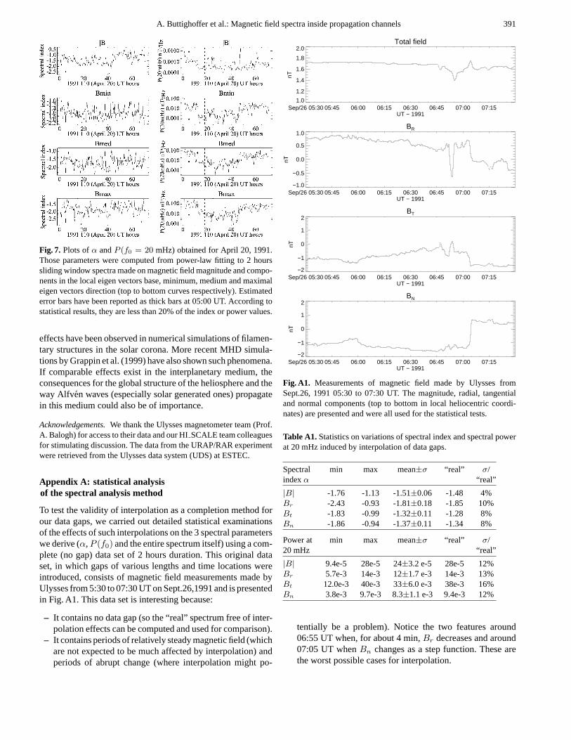
To test the validity of interpolation as a completion method forour data gaps, we carried out detailed statistical examinationsof the effects of such interpolations on the 3 spectral parameterswe derive (α, P (f0) and the entire spectrum itself) using a com-plete (no gap) data set of 2 hours duration. This original dataset, in which gaps of various lengths and time locations wereintroduced, consists of magnetic field measurements made byUlysses from 5:30 to 07:30 UT on Sept.26,1991 and is presentedin Fig. A1. This data set is interesting because:

– It contains no data gap (so the “real” spectrum free of inter-polation effects can be computed and used for comparison).

– It contains periods of relatively steady magnetic field (whichare not expected to be much affected by interpolation) andperiods of abrupt change (where interpolation might po-

Total field

Sep/26 05:30 05:45 06:00 06:15 06:30 06:45 07:00 07:15UT − 1991

1.0

1.2

1.4

1.6

1.8

2.0

nT

BR

Sep/26 05:30 05:45 06:00 06:15 06:30 06:45 07:00 07:15UT − 1991

−1.0

−0.5

0.0

0.5

1.0

nT

BT

Sep/26 05:30 05:45 06:00 06:15 06:30 06:45 07:00 07:15UT − 1991

−2

−1

0

1

2

nTBN

Sep/26 05:30 05:45 06:00 06:15 06:30 06:45 07:00 07:15UT − 1991

−2

−1

0

1

2

nT

Fig. A1. Measurements of magnetic field made by Ulysses fromSept.26, 1991 05:30 to 07:30 UT. The magnitude, radial, tangentialand normal components (top to bottom in local heliocentric coordi-nates) are presented and were all used for the statistical tests.

Table A1. Statistics on variations of spectral index and spectral powerat 20 mHz induced by interpolation of data gaps.

Spectral min max mean±σ “real” σ/indexα “real”

|B| -1.76 -1.13 -1.51±0.06 -1.48 4%Br -2.43 -0.93 -1.81±0.18 -1.85 10%Bt -1.83 -0.99 -1.32±0.11 -1.28 8%Bn -1.86 -0.94 -1.37±0.11 -1.34 8%

Power at min max mean±σ “real” σ/20 mHz “real”

|B| 9.4e-5 28e-5 24±3.2 e-5 28e-5 12%Br 5.7e-3 14e-3 12±1.7 e-3 14e-3 13%Bt 12.0e-3 40e-3 33±6.0 e-3 38e-3 16%Bn 3.8e-3 9.7e-3 8.3±1.1 e-3 9.4e-3 12%

tentially be a problem). Notice the two features around06:55 UT when, for about 4 min,Br decreases and around07:05 UT whenBn changes as a step function. These arethe worst possible cases for interpolation.


|B|

0.1 1.0 10.0 100.0Frequency (mHz)

10-1010-5

100105

Pow

er (

nT2 /H

z)

Br

0.1 1.0 10.0 100.0Frequency (mHz)

10-1010-5

100105

Pow

er (

nT2 /H

z)

Bt

0.1 1.0 10.0 100.0Frequency (mHz)

10-1010-5

100105

Pow

er (

nT2 /H

z)

Bn

0.1 1.0 10.0 100.0Frequency (mHz)

10-1010-5

100105

Pow

er (

nT2 /H

z)|B|

0.1 1.0 10.0 100.0Frequency (mHz)

0.1

1.0

10.0

100.0

Mea

n/R

eal(

-)

Br

0.1 1.0 10.0 100.0Frequency (mHz)

0.11.0

10.0

100.01000.0

Mea

n/R

eal(

-)

Bt

0.1 1.0 10.0 100.0Frequency (mHz)

0.11.0

10.0

100.01000.0

Mea

n/R

eal(

-)

Bn

0.1 1.0 10.0 100.0Frequency (mHz)

0.11.0

10.0

100.01000.0

Mea

n/R

eal(

-)

Fig. A2.Graphical representation of the spectrum variations introducedby interpolation of data gaps. Plots of mean±σ (left hand panels) andmean/real (right hand panels).

The statistical tests consisted of randomly introducing datagaps in the ‘complete’ set to obtain a ‘test’ set. These test sets arethen interpolated and test spectra are computed. Gaps were in-troduced in the following manner: random choice in the locationof 5 data gaps between 05:30 and 07:30 UT and random choiceof their duration (between 0 and 5% of the total duration of thecomplete data set; i.e. gaps of 0 to 6 min duration). We choseto produce test sets which were on average much worse thanthe data sets used in the rest of the study. 1000 such test spectrawere computed. Each of the test spectra was fitted to power-laws in frequencies (from 1 to 40 mHz) from which values ofα andP (f0 =20 mHz) were obtained. For each of the 300 fre-quency points constituting the 1000 test spectra, the minimum,maximum and mean values were computed and compared to the‘real’ values computed from the complete data set. The resultsare presented in Table A1 and shown graphically in Fig. A2.

Listed in Table A1 are the maximum, minimum, mean andstandard deviation values of the spectral indexes and theP (f0 =20 mHz) that were obtained from the 1000 test spectra in the fourmagnetic field time series with various data gaps as describedabove. The actual value of the same quantities from the complete(no gap) time series (Fig. A1) are also listed. Finally, the right–most column gives the ratio of standard deviation to actual valuein percentage.

Plotted by the two lines in each of the left hand panels ofFig. A2, are the mean±σ power spectra for the four magneticfield time series. The difference between each set of 2 linesis small, so no differentiation has been made between them. The

right hand set of panels plots the ratio of the mean spectra to theactual spectrum.

The results (Table A1; Fig. A2) of this statistical study showthat even in the worst possible conditions the standard deviationerrors introduced by the interpolation method using this spec-tral analysis are on the order of, or less than 10% onα and onthe order of, or less than, 16% onP (f0). In terms of the entirepower spectrum, the effect of the interpolation is to producein general a slight order of 10% underestimation of the mini-mal values of the test spectra (hardly visible on the curves) andoccasionally overestimation of the maximal spectral power inlocalized peak frequencies (all major deviations on the mean toactual ratio plots on the right side panels of Fig. A2 are> 1).It is important to note that only a few deviations are more thanone order of magnitude and are observed only at the frequencylocations where a drop in the “real” spectrum occurs. They ap-pear only at discrete frequencies in a few of the test samples.They are striking on the presented curves because the conjunc-tion between the log scale representation and the mean estimatorgives them an artificial importance. In fact, there is no system-atic global deviation of spectra. Therefore, we can say that theinterpolation and the use of this spectral analysis method doesnot create artificial drop-outs or peaks; it may only occasionallydecrease the depth of a few real drop-outs in a non-systematicway. We can conclude that the linear interpolations used to fillthe data gaps (which is very efficient in terms of computationtime) does not introduce excessive bias and is suitable for ouranalysis purpose.

References

Anderson K.A., Dougherty, W.M., 1986, Solar Phys. 103, 165Balogh A., Beek T.J., Forsyth R.J., et al., 1992, A&AS 92, 207Bavassano B., Dobrolwolny M., Fanfoni G., Mariani F., Ness N.F.,

1982a, Solar Phys. 78, 373Bavassano B., Dobrolwolny M., Mariani F., Ness N.F., 1982b, J. Geo-

phys. Res. 87(A5), 3617Beeck J., Wibberenz G., 1986, ApJ 311, 437Buttighoffer A., 1998, A&A 335, 295Buttighoffer A., Pick M., Roelof E.C., et al., 1995, J. Geophys. Res.

100, 3369Davila J.M., 1985, ApJ 291, 328Grappin R., Buttighoffer A., Leorat J., 1999, In: SOHO 8 WorkshopKlein L., Bruno R., Bavassano B., Rosenbauer H., 1993, J. Geophys.

Res. 98(A5), 7837Lanzerotti L.J., Gold R.E., Anderson K.A., et al., 1992, A&AS 92, 207Tan L.C., Mason G.M., 1993, ApJ 409, L29Thomson D.J., 1982, Proceedings of the IEEE 70(9), 1055Tu C.-Y., Marsch E., 1995, Space Sci. Rev. 73, 1Valdes-Galicia J.F., 1993, Space Sci. Rev. 62, 67

astronomy and spectral analysis of the magnetic ﬁeld

Documents