aster level-1 user guide - unit · pdf fileexpressed in latitude/longitude for every block....

ASTER User’s Guide

Part II

Level 1 Data Products

(Ver.5.1)

March, 2007

ERSDAC Earth Remote Sensing Data

Analysis Center

ASTER User’s Guide Part-II (Ver. 5.1) Page-i

ASTER User's Guide Part II

TABLE OF CONTENTS

1. LEVEL-1 PROCESSING AND DATA PRODUCTS OVERVIEW............................................................................... 1

2. LEVEL-1A PROCESSING ALGORITHM ..................................................................................................................... 5 2.1. LEVEL-0 DATA............................................................................................................................................................... 5 2.2. FRONT-END PROCESSING................................................................................................................................................ 6 2.3. RADIOMETRIC CORRECTION........................................................................................................................................... 8 2.4. GEOMETRIC CORRECTION SCHEME .............................................................................................................................. 12 2.5. GEOMETRIC SYSTEM CORRECTION .............................................................................................................................. 13 2.6. PARALLAX CORRECTION.............................................................................................................................................. 20 2.7. INTER-TELESCOPE BAND-TO-BAND REGISTRATION CORRECTION ................................................................................ 22 2.8. GEOMETRIC COEFFICIENTS GENERATION..................................................................................................................... 25 2.9. CLOUD COVERAGE EVALUATION................................................................................................................................. 26

3. LEVEL-1B PROCESSING ALGORITHM.................................................................................................................... 28 3.1. MAP PROJECTION ......................................................................................................................................................... 28 3.2. RESAMPLING ................................................................................................................................................................ 30

4. LEVEL-1A DATA PRODUCT DESCRIPTION ........................................................................................................... 31 4.1. OUTLINE OF CONTENTS................................................................................................................................................ 31 4.2. IMAGE DATA ................................................................................................................................................................ 33 4.3. RADIOMETRIC CORRECTION DATA............................................................................................................................... 35 4.4. GEOMETRIC CORRECTION DATA .................................................................................................................................. 37 4.5. METADATA .................................................................................................................................................................. 38 4.6. SUPPLEMENT DATA...................................................................................................................................................... 38

5. LEVEL-1B DATA PRODUCT DESCRIPTION............................................................................................................ 39 5.1. CONTENTS OF OUTLINE................................................................................................................................................ 39 5.2. IMAGE DATA ................................................................................................................................................................ 41 5.3. RADIOMETRIC PARAMETERS ........................................................................................................................................ 43 5.4. GEOMETRIC PARAMETERS............................................................................................................................................ 46 5.5. GEOLOCATION DATA ................................................................................................................................................... 48 5.6. BAD PIXEL REPLACEMENT METHOD............................................................................................................................ 49 5.7. METADATA .................................................................................................................................................................. 51 5.8. SUPPLEMENT DATA...................................................................................................................................................... 53

6. BROWSE DATA PRODUCTS........................................................................................................................................ 54

7. DATA QUALITY INFORMATION ............................................................................................................................... 56 7.1. REQUIRED QUALITY .................................................................................................................................................... 56 7.2. VALIDATION AND CALIBRATION ACTIVITIES ............................................................................................................... 57 7.3. QUALITY STATUS ........................................................................................................................................................ 59 7.4. GEOLOCATION ERROR INFORMATION 1....................................................................................................................... 60 7.5. GEOLOCATION ERROR INFORMATION 2....................................................................................................................... 62 7.6. CHANGE IN RADIOMETRIC COEFFICIENTS UPDATE METHOD ....................................................................................... 64 7.7. LATEST LEVEL-1A PRODUCTION SYSTEM.................................................................................................................... 66

ASTER User’s Guide Part-II (Ver. 5.1) Page-1

1. Level-1 Processing and Data Products Overview Introduction: ASTER (Advanced Spaceborne Thermal Emission and Reflection Radiometer) is an advanced multispectral sensor that is a facility instrument selected by NASA to fly on the Terra polar orbiting spacecraft in December 1999, and covers a wide spectral region from visible to thermal infrared with 14 spectral bands with high spatial, spectral and radiometric resolution. The spectral bandpasses are shown in Table 2-1. The wide spectral region is covered by three telescopes, three VNIR (Visible and Near Infrared Radiometer) bands with a spatial resolution of 15 m, six SWIR (Short Wave Infrared Radiometer) bands with a spatial resolution of 30 m and five TIR (Thermal Infrared Radiometer) bands with a spatial resolution of 90 m. In addition one more telescope is used to see backward in the near infrared spectral band (band 3B) for stereoscopic capability that will produce a base-to-height ratio of 0.6. Please refer to Volume I for more details on the ASTER instrument and the science objective. This multi-telescope configuration necessitates inter-telescope band-to-band registration with an image matching technique in the Level-1 algorithm. The intra-telescope band-to-band registration for the SWIR bands is also carried out with the image matching technique to remove the parallax error due to the detector distribution on the focal plane. The ASTER instrument has two types of Level-1 data, Level-1A and Level-1B data. Level-1A data are formally defined as reconstructed, unprocessed instrument data at full resolution. According to this definition the ASTER Level-1A data consist of the image data, the radiometric coefficients, the geometric coefficients and other auxiliary data without applying the coefficients to the image data to maintain the original data values. The Level-1B data are generated by applying these coefficients for radiometric calibration and geometric resampling. All acquired image data are required to be produced to Level-1A. The ASTER Ground Data System (ASTER GDS) must handle a large amount of data, because the ASTER instrument has a high spatial resolution. The average data rate allocated to the ASTER instrument is limited to 8.3 Mbps which roughly corresponds to a duty cycle of 8 %. S Therefore, the maximum daily data volume which the ASTER GDS must handle is 780 sets of 60 km x 60 km scenes and corresponds to about 80 GB daily. A maximum of 310 scenes per day are to be processed to Level-1B data in response to requests from users.


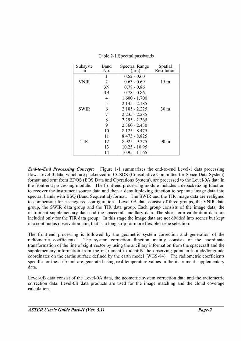
Table 2-1 Spectral passbands

Subsystem

Band No.

Spectral Range (µm)

Spatial Resolution

1 0.52 - 0.60 VNIR 2 0.63 - 0.69 15 m

3N 0.78 - 0.86 3B 0.78 - 0.86 4 1.600 - 1.700 5 2.145 - 2.185

SWIR 6 2.185 - 2.225 30 m 7 2.235 - 2.285 8 2.295 - 2.365 9 2.360 - 2.430 10 8.125 - 8.475 11 8.475 - 8.825

TIR 12 8.925 - 9.275 90 m 13 10.25 - 10.95 14 10.95 - 11.65

End-to-End Processing Concept: Figure 1-1 summarizes the end-to-end Level-1 data processing flow. Level-0 data, which are packetized in CCSDS (Consultative Committee for Space Data System) format and sent from EDOS (EOS Data and Operations System), are processed to the Level-0A data in the front-end processing module. The front-end processing module includes a depacketizing function to recover the instrument source data and then a demultiplexing function to separate image data into spectral bands with BSQ (Band Sequential) format. The SWIR and the TIR image data are realigned to compensate for a staggered configuration. Level-0A data consist of three groups, the VNIR data group, the SWIR data group and the TIR data group. Each group consists of the image data, the instrument supplementary data and the spacecraft ancillary data. The short term calibration data are included only for the TIR data group. In this stage the image data are not divided into scenes but kept in a continuous observation unit, that is, a long strip for more flexible scene selection. The front-end processing is followed by the geometric system correction and generation of the radiometric coefficients. The system correction function mainly consists of the coordinate transformation of the line of sight vector by using the ancillary information from the spacecraft and the supplementary information from the instrument to identify the observing point in latitude/longitude coordinates on the earths surface defined by the earth model (WGS-84). The radiometric coefficients specific for the strip unit are generated using real temperature values in the instrument supplementary data. Level-0B data consist of the Level-0A data, the geometric system correction data and the radiometric correction data. Level-0B data products are used for the image matching and the cloud coverage calculation.


The SWIR parallax error is caused by the offset in detector alignment in the along-track direction (Figure 8a) and depends on the distance between the spacecraft and the observed earths surface. For SWIR bands the parallax error corrections are carried out with the image matching technique or the coarse DEM data base depending on cloud coverage, by using Level-0B data. For SWIR and TIR bands, the inter-telescope registration correction is carried out with VNIR band 2. The correction coefficient is evaluated by image matching between bands 2 and 6 for SWIR bands and between bands 2 and 11 for TIR bands. The scene cutting is carried out on Level-0B data, according to the predetermined World Reference System (WRS). Each group of data are divided into scenes of 60 km in the along-track direction but includes 3 more km of data to provide an overlap of 5 % with neighboring scenes except for backward stereo band 3B. For band 3B the scene size is 81 km, including an additional overlap of 6 km to compensate for the terrain error contribution and a scene rotation for a large cross-track pointing All geometric correction processes and scene cutting process are followed by a set of geolocation data generated for each scene. All geometric information is consolidated into a set of geolocation data expressed in latitude/longitude for every block. The Level-1A data product consists of the image data, the radiometric coefficients, the geolocation data and the auxiliary data. The Level-1B data product can be generated by applying these data for radiometric calibration and geometric resampling.


BAND 2

BAND 4

BANDS 6 & 7

CLOUD COVERAGE CALCULATION

SWIR GEOMETRIC SYSTEM CORRECTION

SWIR PARALLAX CORRECTION

ANCILLARY DATA

SW IR SUPPLEMENT DATA

ANCILLARY DATA

VNIR SUPPLEMENT DATA

ANCILLARY DATA

TIR SUPPLEMENT DATA

TIR GEOMETRIC SYSTEM CORRECTION

EDOS

SW IR/VNIR INTER-TELESCOPE GEOMETRIC CORRECTION

BAND 2

BAND 6

TIR/VNIR INTER-TELESCOPE GEOMETRIC CORRECTION

BAND 2

BAND 11

ASTER LEVEL-1A DATA PRODUCTS

ASTER LEVEL-1B DATA PRODUCTS

V/G-DB; VNIR geometric correction data base file V/R-DB; VNIR radiometric correction data base file S/G-DB; SWIR geometric correction data base file S/R-DB; SWIR radiometric correction data base file T/G-DB; TIR geometric correction data base file T/R-DB; TIR radiometric correction data base fileUS

JAPAN PHYSICAL OR ELECTRONIC

RADIOMETRIC CALIBRATION GEOMETRIC RESAMPLING

VNIR L-1A DATA

BAND 11

EARTH MODEL

EARTH MODEL

EARTH MODEL

SW IR L-1A DATA

TIR L-1A DATA

VNIR GEOMETRIC COEFFICIENTS GENERATION

SW IR GEOMETRIC COEFFICIENTS GENERATION

TIR GEOMETRIC COEFFICIENTS GENERATION

DEMULTIPLEXING

VNIR 1&2 DATA FILE

DEPACKETIZING

4 TIR BANDSSW IR BANDS

VNIR BANDS 3N & 3BVNIR BANDS 1 & 2

INSTRUMENT SOURCE DATA

1

32

4 SHORT TERM CALIBRATION DATA

VNIR RADIOMETRIC COEFFICIENTS GENERATION

VNIR SCENE CUTTING

TIR SCENE CUTTING

STAGGER REALIGNMENT

SWIR RADIOMETRIC COEFFICIENTS GENERATION

TIR RADIOMETRIC COEFFICIENTS GENERATION

VNIR L-0B DATA

SW IR L-0B DATA

TIR L-0B DATA

CLOUD COVERAGE DATA

STAGGER REALIGNMENT

SWIR SCENE CUTTING

DC CLAMP CORRECTION

CCSDS L-0 DATA

CCSDS PACKET

CCSDS PACKETCCSDS

PACKETCCSDS PACKET

CCSDS PACKET

CCSDS PACKETCCSDS

PACKET

TIR 10-14 DATA FILE

CCSDS PACKET

CCSDS PACKETCCSDS

PACKETCCSDS PACKET

CCSDS PACKET

CCSDS PACKET

CCSDS PACKET

SWIR 4-9 DATA FILE

CCSDS PACKET

CCSDS PACKET

CCSDS PACKET

CCSDS PACKET

CCSDS PACKETCCSDS

PACKETCCSDS PACKET

VNIR 3N & 3B DATA FILEVNIR I&2

DATA FILE

CCSDS PACKET

CCSDS PACKET

CCSDS PACKET

CCSDS PACKETCCSDS

PACKETCCSDS PACKET

CCSDS PACKET

VNIR GEOMETRIC SYSTEM CORRECTION

TIR L-0A IMAGE DATA 14 13 12 11 10

9 8 7 6 5 4

SW IR L-0A IMAGE DATA

3B 3N 2 1

VNIR L-0A IMAGE DATA

V/G-DB

S/G-DB

T/G-DB

T/R-DB

S/R-DB

V/R-DB

MAP PROJECTION

Figure 1-1 Summarized end-to-end processing folw


2. Level-1A Processing Algorithm 2.1. Level-0 Data Level-0 Production Data Set: The Level-0 data which are sent from EDOS are packetized in the CCSDS format as shown in Figure 2-1. These packets are classified into four groups of data according to an APID (Application Process Identification) in the primary header of each packet. The group 1 data contain the data for VNIR bands 1 and 2. The group 2 data contain the data for VNIR bands 3N and 3B. The group 3 data contain the data for all SWIR bands. The group 4 data contain the data for all TIR bands. Each data group include science image data, instrument supplement data and spacecraft ancillary data. ASTER is allocated the 64 APIDs that lie within the decimal equivalent range of 256 - 319. Different APIDs are allocated depending on data content (image data, instrument supplement data, or spacecraft ancillary data), data groups and operation modes (observation mode, calibration mode and test mode). The packets are sorted out with the time tag data in the secondary header and then sorted out in the order of the image data, the instrument supplement data and the spacecraft ancillary data with different APIDs. Some packets contain both the supplement data and the ancillary data in the same packet. In a group with the same APID the packets are sorted out in the order of sequential counter data in the primary header.

VERSIONTYPE SEC HDR FLG

APPLIC. PROC. ID

SEQUENCE FLAGS

PACKET SEQUENCE COUNT

PACKET LENGTHSECONDARY HEADER

INSTRUMENT DATA FIELD

PACKET IDENTIFICATION PACKET SEQUENCE CONTROL

TIME TAGQUICK LOOK FLAG

"000"

3 BITS

"0"

1 BIT 1 BIT 11 BITS 2 BITS 14 BITS

"00"=Cont'd "01"= 1 st "10"= Last "11"= Unsegm data

16 BITS 64 BITS 8 BITS

VARIABLE LENGTH

PRIMARY HEADER 48 BITS (6 OCTETS)

72 BITS (9 OCTETS)

DAY

"0"1 BIT 15 BITS

ms OF DAY µs OF ms

32 BITS 16 BITS

Q SUPPLIED BY PACKET SOUR

1 7

Q="0" ; PACKET NOT FOR QUICK LOOK DAQ="1" ; PACKET FOR QUICK LOOK DATA SE

Figure 2-1 CCSDS Level-0 data packet format


2.2. Front-end Processing Depacketizing of CCSDS Level-0 Data: The packets of each group are depacketized and aligned to recover the unpacketized instrument source data by using a sequential counter, flags in the primary header and time tags in the secondary header. In the instrument source data format, the spectral band information is multiplexed with the image in BIP (Band Interleaved by Pixel) format as shown in Figure 2-2. Each swath line of image data is appended by the instrument supplement data and spacecraft ancillary data specific for the swath line.

VNIR (1): Bands 1 & 2IMAGE DATA (BIP FORMAT) VNIR SUPPLEMENT DATAANCILLARY DAT

400 BITS 512 BITS65,600 BITS

SWIR: Bands 4 - 9IMAGE DATA (BIP FORMAT) SWIR SUPPLEMENT DATAANCILLARY DATA

328 BITS 98,304 BITS 512 BITS

TIR: Bands 10 - 14IMAGE DATA (BIP FORMAT) TIR SUPPLEMENT DATAANCILLARY DATA

453,120 BITS 79,312 BITS 512 BITS

65,600 BITS

VNIR (2): Bands 3N & 3BIMAGE DATA (BIP FOMAT) VNIR SUPPLEMENT DATAANCILLARY DAT

400 BITS 512 BITS65,600 BITS

Figure 2-2 Instrument source data format Demulitplexing Instrument Source Data: The instrument source data are demultiplexed to separate image data for every spectral band into BSQ (Band Sequential) format. Here, we have the data rearranged in three groups, that is, the VNIR data group, the SWIR data group and the TIR data group. Each data group consists of the image data for each spectral band, the supplement data and the ancillary data. For only the TIR data group, the short term calibration obtained at the beginning of each observation is included. The supplementary data are necessary for all of the data groups to make it possible to process them independently. In this stage the image data are not divided into scenes but kept in one continuous observation unit, that is, a long strip of image data for more flexible scene selection. This data set is defined as Level-0A data which is a tentative product only used during processing.


Image Data Stagger Realignment: For SWIR and TIR image data the Level-0 pixel addresses are changed, so that all pixels for each band lie on one line, compensating for the staggered configuration described below. This realignment process is carried out not only to have more exactly aligned image data without resampling for the image matching process but also to simplify subsequent processes. The SWIR subsystem uses electronically scanned linear detector arrays for each band to obtain one data line simultaneously in the cross-track direction for each scan period. These detector arrays are separated for odd and even numbered detectors with a staggered configuration as shown in Figure 2-3(a). The realignment for SWIR pixel addresses is carried out to compensate for the difference from the center line between the odd and the even lines. The stagger offset value to the center line can be set to ±1 pixel with a good approximation. TIR images are obtained by mechanical scanning with 10 detectors for each spectral band, that is, 50 detectors in total. Ten detectors for each band are arranged with the staggered configuration in the cross-track direction as shown in Figure 2-3(b). The realignment for TIR pixel addresses is carried out to compensate for the difference from the center line between the odd and the even lines. The stagger offset value to the center line can be set to ±4 pixels with a good approximation.

1

2

3

4

5

-1 PIXEL

+1 PIXEL

••••••••••

••••••••

(a) SWIR

1

2

3

4

5

6

7

8

9

10

+4 PIXELS-4 PIXELS

(b) TIR

Flight Direction

Flight Direction

Figure 2-3 Realignment positions of staggered SWIR and TIR pixels


2.3. Radiometric Correction Common: Radiometric coefficients are generated in two steps. The first step is an off-line process from Level-1 data product generation to prepare radiometric coefficients at predefined reference temperature. These coefficients will be effective for a long time, depending on the instrument stability, and available in radiometric correction data base files along with the temperature coefficients. One set of offset and sensitivity data are necessary for the VNIR and SWIR bands and one set of offset, linear sensitivity and nonlinear sensitivity data are necessary for the TIR bands. Destriping parameters will be generated from the image data if necessary, analyzing the image data obtained during the initial checkout operation period. The second step is an on-line process executed during Level-1 product generation to correct the radiometric coefficients for instrument conditions such as detector temperature and dewar temperature, which may change for every observation. Destriping parameters will be generated from the image data if necessary, analyzing the image data obtained during the initial checkout operation period. Generation of Radiometric Correction Data Base: The radiometric coefficients for the reference temperatures were evaluated during the preflight test period using integration spheres, followed by a regular evaluation during the inflight period with on-board calibration and vicarious calibration data, and then updated if necessary. On-board calibration is scheduled every 17 days to check the stability. These radiometric coefficients are available in the radiometric correction data base with temperature coefficients as on-line parameter files applied in the Level-1 processing. All temperature coefficients were prepared during the preflight test period and will be used throughout the mission period. The required absolute accuracies are 4% (σ) for VNIR and SWIR, and 1 to 3K for TIR depending on target temperatures. Generation of VNIR Observation-Unit-Specific Radiometric Coefficients: Figure 2-4(a) shows the VNIR radiometric coefficients generation algorithm flow. Detector temperature is the only reference parameter by which the radiometric coefficients (offset and sensitivity) have to be corrected for a specific observation unit data set. Under normal operating conditions within the designed temperature range, this correction process will not be necessary, since the correction value is expected to be very small Generation of SWIR Observation-Unit-Specific Radiometric Coefficients: Figure 2-4(b) shows the SWIR radiometric coefficients generation algorithm flow. Detector temperature and dewar temperature are the reference parameters by which the radiometric coefficients (offset and sensitivity) have to be corrected for a specific observation unit data. Under normal operating conditions the detector temperature is controlled to within ±0.2 K at around 77 K. Therefore the correction process for detector temperature will not be necessary as long as the SWIR is operating normally . The dewar temperature correction, which is necessary for compensating only for thermal radiation from the dewar, is applied only to the offset, since the SWIR detector is sensitive to room temperature


thermal radiation up to 5 µm and the band pass filter can not completely remove this out-of-band radiation. The dewar temperature is used as a representative value for the internal thermal radiation. Generation of TIR Observation-Unit-Specific Radiometric Coefficients: Figure 2-4(c) shows the TIR radiometric coefficients generation algorithm flow. The linear and the non-linear sensitivities coefficients in the data base are corrected only by the detector temperature. Under normal operating conditions the detector temperature is within ±0.2 K at around 80 K. Therefore, correction for the detector temperature will not be necessary as long as TIR is operating normally. The offset data, common throughout the observation unit, are generated from the short term calibration data acquired at the beginning of each observation by using the blackbody temperature in the TIR supplementary data. The correction for the offset data due to chopper temperature is calculated using the chopper temperature changes from the short term calibration period. The chopper temperature correction is carried out on the TIR Level-0A image data with the DC clamp correction. This correction will be possible for each scan data (each ten lines of data in the along-track direction), since the chopper temperature data is included in the supplementary data. This image data correction will result in slightly different TIR Level-0B image data DN values from Level-0 data. The Level-0 data is digitized to 12 bits. The LSB (Least Significant Bit) value of Level-0B image data is very small compared to NE∆T (less than one third for the 300 K target). Therefore, this difference will not give rise to any significant round-off error.


(a) VNIR


V/R-DB

• DETECTOR TEMPERATURE • GAIN STATUS

TO VNIR L-0B DATA


OFFSET CORRECTION SENSITIVITY CORRECTION

DESTRIPING PARAMETERS GENERATION

VNIR IMAGE DATA

(b) SWIR

S/R-DB

• DETECTOR TEMPERATURE • DEWAR TEMPERATURE • GAIN STATUS

TO SWIR L-0B DATA

SWIR SUPPLEMENT DATA

OFFSET CORRECTION SENSITIVITY CORRECTION



SWIR IMAGE DATA

OFFSET DATA CALCULATION

LINEAR SENSITIVITY CORRECTION

NON-LINEAR SENSITIVITY CORRECTION

TO TIR L-0B DATA

SHORT TERM CALIBRATION DATA

T/R-DB

DETECTOR TEMPERATURE

DETECTOR TEMPERATURE

• BLACKBODY TEMPERATURE • CHOPPER TEMPERATURE

TIR SUPPLEMENT DATA

OFFSET DATA

CHOPPER TEMPERATURE CORRECTION VALUE CALCULATION

CHOPPER TEMPERATURE

Note A/T-LATTICE POINT: Lattice point in along-track direction


TIR IMAGE DATA

IMAGE DATA DN VALUECORRECTION

(EVERY SCAN LINE)

DC CLAMP CORRECTIONDATA

TIR L0B IMAGE DAT

(c) TIR

Figure 2-4 Radiometric correction coefficients generation flow


TIR DC Clamp Correction: TIR output voltage is clamped at -1.4 V ± ∆Vn for bands 10-12 and -0.9 V± ∆Vn for bands 13 and 14 when the chopper plate is observed by the detectors at every scan. The small voltage ∆Vn is the noise voltage at the moment of the clamp which changes randomly in every scan and must be corrected to exactly set the clamp voltage. Figure 2-5 shows the TIR DC clamp correction flow. The exact clamped output (DN value) is available in the TIR supplementary data as the chopper data. The chopper data in the one previous scan are used for the correction. The 100 chopper data acquired for one scan are averaged to reduce noise component, followed by the DC clamp error calculation which corresponds to ± ∆Vn . This clamp error is transferred to the TIR radiometric correction module to subtract it from the TIR Level-0A image data to generate Level-0B image data.

TIR SUPPLEMENT DATA

CHOPPER DATA

CHOPPER DATA AVERAGING

DC CLAMP ERROR CALCULATION

ONE PREVIOUS CHOPPER DATA SELECTI

TO RADIOMETRIC COEFFICIENTS GENERAT

Figure 2-5 TIR DC clamp correction


2.4. Geometric Correction Scheme Common: The geometric correction process consists of three steps. The first step is an off-line process from Level-1 data product generation to prepare geometric parameters such as the line-of-sight vectors of detectors and the pointing axes information. These parameters are effective for a long time, depending on the instrument stability, and are recorded in the geometric correction data base files. The second step is an on-line process executed during Level-1 product generation to identify the observing points of detectors, using the geometric parameters available in the geometric correction data base files and the engineering information supplied by the instrument and the spacecraft. This process is called “Geometric System Correction”. The third step is also an on-line process to enhance band-to-band registration accuracy by image matching techniques. This step consists of two parts. One is the SWIR parallax correction process. Another is the inter-telescope registration process. Generation of Geometric Correction Data Base: The geometric correction data base files contain the line-of-sight vectors of the detectors, the pointing axis vectors and the conversion coefficients from encoder values to angles. The line-of-sight vectors of the detectors and the pointing axis vectors were evaluated toward the Navigation Base Reference of the spacecraft during the preflight test period using the collimator data and the alignment data on the spacecraft. These geometric parameters will be corrected after launch through the validation activity using GCPs (Ground Control Points) and band-to-band image matching techniques.


2.5. Geometric System Correction General Description: The geometric system correction is the rotation and the coordinate transformation of the line of sight vectors of detectors to the earth Greenwich coordinate system using only the engineering information from the instrument and the spacecraft to identify the observed points by the detectors. The observed point on the surface is identified by the intersection of the earths surface and an extended line-of-sight vector. The engineering information from the instrument and the spacecraft are called the supplementary data and the ancillary data, respectively. The geometric system correction is almost the same for the three subsystems, except for selected numbers of vectors to be transformed. Figure 2-6 shows the geometric system correction flow. The image data are divided into blocks for both the cross-track and the along-track directions. The block sizes are as follows. VNIR bands 1, 2, 3N: 410 x 400 pixels VNIR band 3B: 500 x 400 pixels SWIR all bands: 20 x 20 pixels TIR all bands: 72 x 70 pixels These values were decided by considering the distortion of optical images on the focal plane in the cross-track direction and spacecraft stability in the along-track direction. The coordinate transformations are carried out only for the line-of-sight vectors of selected detectors. The numbers of the selected detectors are 11, 104 and 11 for VNIR, SWIR and TIR bands, respectively, which correspond to the number of the corner for each block of Level-0 images in the cross-track direction. Dummy detectors will have to be introduced to compensate for and then to completely define the block at the end of the cross-track direction. The geometric system correction is divided into several parts as follows: (1) The pointing correction (2) The coordinate transformation from Navigation Base Reference of the spacecraft to the Orbital

Reference Frame (3) The coordinate transformation from the Orbital Reference Coordinate Frame to the Earth Inertial

coordinate Frame (4) The coordinate transformation from the Earth Inertial Coordinate Frame to the Earth Greenwich

Coordinate Frame (5) Identification of the intersection of the Earth surface and an extension of the line of sight vector


FORB FINE

V/G-DB

ANCILLARY DATA

EARTH ROTATION CALCULATION

POINTING POSITION POINTING KNOWLEDGE

EARTH MODEL (WGS-84)


LINE OF SIGHT VECTORS OF SELECTED DETECTORS 11 FOR VNIR 104 FOR SWIR 11 FOR TIR

ATTITUDE ANGLES ATTITUDE RATES

TO *

FROM *

TO **

FROM**

COORDINATE SYSTEM TRANSFORMATION (1)

SPACECRAFT COORDINATES

ORBIT COORDINATES

ΦS/C ΦORB

GEOLOCATION DATA

POINTING CORRECTION

POSITION (LATITUDE. LONGITUDE)

POSITION, VELOCITY

TIME STAMP TIME CONVERSION

COORDINATE SYSTEM TRANSFORMATION (2-N)ΦORB ΦINEORBIT COORDINATES

EARTH INERTIAL COORDINATES

COORDINATE SYSTEM TRANSFORMATION (2-2)ΦORB Φ INE

ORBIT COORDINATES


COORDINATE SYSTEM TRANSFORMATION (2-1)ΦORB ΦINEORBIT COORDINATES


Φ INECOORDINATE SYSTEM TRANSFORMATION (3-N)

ΦGREEARTH INERTIAL COORDINATES

EARTH GREENWICH COORDINATES

COORDINATE SYSTEM TRANSFORMATION (3-2)ΦINE ΦGRE



COORDINATE SYSTEM TRANSFORMATION (3-1)ΦGRE



Φ INE

ΦGRE ΦLLOBSERVATION POINT IDENTIFICATION


LATITUDE/LONGITUDE COORDINATES

POINTING AXIS VECTOR

Figure 2-6 Geometric system correction flow


Pointing Correction : The line of sight vectors in the geometric data base are those for the reference pointing angles (nominal nadir direction). The line of sight vectors are changed using the pointing position and knowledge from the supplementary data. The pointing axes information in the geometric data base are used for the transformation of the line-of-sight vectors due to change in the pointing position. The line of sight vector changes with the rotation for the pointing axis by an angle of β from S0 to S as follows.

SX

SY

SZ

S0X

S0Y

S0Z

=

1 0 0

0 cos β -sin β

0 sin β cos βM-1 M

(2-1) where S0x, S0y, S0z : x, y , z components of the line of sight vector S0 befor pointing, Sx, Sy, Sz : x, y, x components of the line of sight vector S after pointing,

M ≡

cos θpitch 0 -sin θpitch

0 1 0

sin θpitch 0 cos θpitch

cos θyaw sin θyaw 0

-sin θyaw cos θyaw 0

0 0 1 , (2-2)

M-1 ≡

cos θpitch 0 sin θpitch

0 1 0

-sin θpitch 0 cos θpitch

cos θyaw -sin θyaw 0

sin θyaw cos θyaw 0

0 0 1 , (2-3) ∆θyaw ≡ sin-1(Py ) , (2-4) ∆θpitch ≡ -tan-1(Pz /Px ) , (2-5) Px, Py, Pz : x, y, z componets of the pointing axes unit vector in the NBR Coordinate Frame. Figure 2-7 shows the relation between the pointing axis and the NBR Coordinate Frame. The angles ∆θyaw and ∆θpitch are the yaw and the pitch rotation angles, respectively, to coalign the XNBR to the pointing axis.


Px

PyPz

YNBR

XNBR

ZNBR

Pointing Axis Unit VectorPax

Perpendicular line from Pax to XNBR ZNBRplane

∆θyaw

∆θpitch

∆θyaw = sin-1(Py) ∆θpitch = -tan-1(Pz /Px)

Figure 2-7 Pointing Axis Vector in NBR Coordinate Frame Spacecraft-to-Orbit Coordinates : The spacecraft coordinates are slightly different from the orbit coordinates. The difference originates from the spacecraft attitude control accuracy and is provided as the attitude angle data in the spacecraft ancillary information. The orbit coordinate system is right-handed and orthogonal. The +z-axis is a line from the spacecraft center of mass to the center of the earth. The +y-axis is a line normal to the z-axis and the spacecraft instantaneous velocity vector (negative orbit normal direction). The x-axis completes the right hand set. This process is carried out by using attitude angles and rates in the ancillary data. The line of sight vectors in the Spacecraft NBR Coordinate Frame can be converted to the expression in the Orbital Reference Frame using the attitude angle data in the spacecraft ancillary data as follows. SOR = FSO•yaw FSO•pitch FSO•roll S , (2-6) where S : the line of sight vector expressed in the NBR Coordinate Frame, SOR : the line of sight vector expressed in the Orbit Reference Coordinate Frame,

1 0 0

0 cos (-αroll) sin (-αroll)

0 -sin (-αroll) cos (-αroll)

FSO•roll ≡

, (2-7)

cos (-αpitch) 0 -sin (-αpitch)

0 1 0

sin (-αpitch) 0 cos (-αpitch)

FSO•pitch ≡

, (2-8)


cos (-αyaw) sin (-αyaw) 0

-sin(-αyaw) cos(-αyaw) 0

0 0 1

FSO•yaw ≡

, (2-9) αroll, αpitch , αyaw : roll, pitch, yaw components of the attitude data, respectively, in the spacecraft ancillary data Orbit-to-Earth Inertial Coordinates : This process is the coordinate transformation to earth-centered coordinates in inertial space. Two-dimensional array vectors can be obtained by this transformation using the spacecraft movement. The array dimension for one observation depends on each observation period, that is, number of pixels in the along-track direction. This process is carried out by using position and velocity information in the ancillary data. The Precession and the Nutation effects are considered to be the more accurate geolocation data, since the spacecraft position information is based on the mean of the J2000.0 coordinate frame, which is the earth inertial coordinates at noon of January 1st, 2000. The line of sight vectors in the Orbital Reference Coordinate Frame can be converted to the expression in the Earth Inertial Coordinate Frame as follows. SEI = FOI SOR, (2-10) where SOR : the line of sight vector expressed in the Orbit Reference Coordinate Frame, SEI : the line of sight vector expressed in the Eartt Inertial Coordinate Frame, FOI ≡ (Tx Ty Tz ), (2-11) Tx Ty Tz : unit vector components of x, y and z axes of the Orbital Coordinate Frame expressed in the Earth Inertial Coordinate Frame and defined as Tx ≡ Ty x Tz Ty ≡ unit (-R x V ) (2-12) Tz ≡ unit (-R ) R ,V : the spacecraft position and velocity vectors expressed in the Earth Inertial Frame For more accurate calculation the Precession matrix P and the Nutation matrix N shall be applied to the line of sight vector SEI in the Earth Inertial Coordinate Frame.


Earth Inertial-to-Earth Fixed coordinates : This process is the coordinate transformation to the earth centered and earth-fixed coordinates, and carried out by using the earth rotation values calculated from the time information in the ancillary data. The UTC time, which is provided from the spacecraft, is converted to the UT1 to calculate the exact earth rotation angle. The line of sight vectors in the Earth Inertial Coordinate Frame can be converted to the expression in the Earth Fixed Coordinate Frame as follows. SEF= FIF SEI , (2-13) where SEI : the line of sight vector expressed in the Eartt Inertial Coordinate Frame, SEF : the line of sight vector expressed in the Eartt Fixed Coordinate Frame,

cos θg sin θg 0

-sinθg cosθg 0

0 0 1

FIF ≡

, (2-14) θg : Greenwich true sidereal hour angle. Earth Surface Identification : The observation point is identified from the intersection of the earth surface and an extension of the line-of-sight vector. The WGS-84 is used as the earth surface model. The observing earth surface can be identified calculating the crossing point between the extension line of the LOS vector and the earth surface. The extension line of the LOS vector can be expressed as follows. x = X + SEF•x r y = Y + SEF•y r (2-15) z = Z + SEF•z r where SEF•x , SEF•y , SEF•z : x, y, z components of the LOS vector SEF in the Earth Fixed Coordinate Frame, X, Y, Z : x, y, z components of the Spacecraft position vector in the Earth Fixed Coordinate Frame r : parameter. The earth surface can be expressed as follows. (x 2 + y 2)/a 2 + z 2/b 2 = 1, (2-16) where a = 6378136m (Earth radius at equator--WGS-84), b = a (1 - f ) (Earth radius at pole----WGS-84), (2-17)


f = 1/298.2572 . The intersection can be calculated from eqs.(2-15) and (2-16). When the observing point is expressed as Px, Py, and Pz , the geocentric latitude ψ and the longitude λ can be expressed as follows. ψ = tan-1Pz /(Px

2 + Py2)1/2, (2-18)

λ = tan-1(Py /Px ) . (2-19) System Correction Accuracy : Table 2-2 shows the pixel geolocation knowledge as a result of the geometric system correction considering both the spacecraft and the instrument contributions. Total ASTER pixel geolocation knowledge is decided by the spacecraft position knowledge, the spacecraft pointing knowledge and ASTER pointing knowledge. Only the pixel geolocation knowledge of VNIR is considered, since the SWIR and TIR bands will be coregistered to VNIR band 2 as a reference band in the Level-1 processing.

Table 2-2 Pixel Geolocation Knowledge

Specification Dynamic Error (3σ)

Static Error (3σ)

Spacecraft*1 ±342 ±28 ±111 Along-track (m) ASTER/VNIR ±205 ±38 ±99 Total ±431*2 ±47 ±149 Spacecraft*1 ±342 ±25 ±148 Cross-track (m) ASTER/VNIR ±205 ±48 ±103 Total ±437*2 ±54 ±180

*1: Three non-optimal 9 minute TDRS contacts per orbit, GJM2 Geopotential ( 30 x 30), solar flux of 175, 5 % Cd error, TDRS ephemeris error of 75 meters. Two star trackers, rigid body/low frequency pointing knowledge error removed *2: Slightly larger than RSS of two values (Spacecraft and ASTER instrument), because of unallocated margin. The geometric system correction accuracy will be regularly checked through the geometric validation activity using GCPs during the normal operation period.


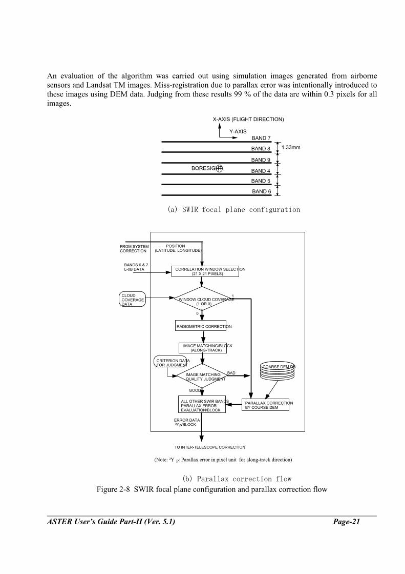
2.6. Parallax Correction The large offset among SWIR bands in the along-track direction shown in Figure 2-88(a) gives rise to parallax errors for band-to-band registration depending on the distance between the instrument and the targeted ground. The algorithm used for SWIR intra-telescope registration is a combination of the image matching correlation method and the coarse DEM method. The ETOPO-030 prepared by EROS Data Center will be used as the coarse DEM. A criterion of selecting band for image matching is good correlation, consequently spectrally close. Bands 6 and 7 are selected, although any other combination of neighbouring bands in the 2µm region will be available for this purpose. As shown in Figure 8(a), detector arrays of bands 6 and 7 are located at opposite ends of the focal plane to increase the parallax detection sensitivity. Figure 2-8(b) shows the parallax correction flow. In order to eliminate this band-to-band misregistration due to the parallax, the SWIR parallax correction process handles the image data as follows.

(1) Select band 7 as a moving window image and band 6 as a target image. The moving window is selected such that its center corresponds to the lattice point at which the geometric system correction is carried out. The target image is selected to cover the search area. The moving window image (band 7) size is 21 by 21 pixel.

(2) Select only cloud free windows for the correlation. Use the coarse DEM data for cloudy

windows. (3) Carry out the radiometric correction for the two window images (4) Find correlation coefficients by moving the window in the along-track direction. (5) Find the highest correlation point in sub-pixel units by interpolating the correlation data

calculated in pixel units. (6) Evaluate the image matching quality. Criteria for judgment are the correlation coefficient and

the deviation from the predetermined value from the coarse DEM data. The threshold value for the correlation coefficient and the threshold deviation for the predetermined value are set to 0.7 and 20% deviation, respectively, in the initial stage. Use the parallax errors calculated by the coarse DEM if the image matching quality can not meet the criterion mentioned above.

(7) Evaluate the parallax error of all SWIR bands for the nadir direction.

The registration error due to the parallax is evaluated at every lattice point (the corner point of the block) and expressed with the pixel unit for the Level-0B image data in the along-track direction.


An evaluation of the algorithm was carried out using simulation images generated from airborne sensors and Landsat TM images. Miss-registration due to parallax error was intentionally introduced to these images using DEM data. Judging from these results 99 % of the data are within 0.3 pixels for all images.

CORRELATION WINDOW SELECTION (21 X 21 PIXELS)

WINDOW CLOUD COVERAGE (1 OR 0)

RADIOMETRIC CORRECTION

IMAGE MATCHING/BLOCK (ALONG-TRACK)

IMAGE MATCHING QUALITY JUDGMENT

ALL OTHER SWIR BANDS PARALLAX ERROR EVALUATION/BLOCK

PARALLAX CORRECTION BY COURSE DEM

CLOUD COVERAGE DATA

COARSE DEM DB

FROM SYSTEM CORRECTION

TO INTER-TELESCOPE CORRECTION

ERROR DATA ²YP/BLOCK

GOOD

BAD

POSITION (LATITUDE, LONGITUDE)

BANDS 6 & 7 L-0B DATA

(Note: ²Y P: Parallax error in pixel unit for along-track direction)

1

0

CRITERION DATA FOR JUDGMENT

X-AXIS (FLIGHT DIRECTION)

1.33mm

BORESIGHT

BAND 7

BAND 8

BAND 9

BAND 4

BAND 5

BAND 6

Y-AXIS

(a) SWIR focal plane configuration

(b) Parallax correction flow Figure 2-8 SWIR focal plane configuration and parallax correction flow


2.7. Inter-telescope Band-to-band Registration Correction The ASTER instrument configuration with the multi-telescopes necessitates routine processing for the inter-telescope band-to-band registration on the ground, unless the boresights are stable enough during the mission life to keep the initial state after launch. The pointing change mechanism is also a source of misregistration because of limited accuracy of pointing position knowledge. The important feature to be stressed here for the inter-telescope registration is that a set of correction parameters will be valid and can be applied to all images as long as the pointing is kept at the same position and the elapsed time since a previous parameter setting is short enough for boresight stability. The inter-telescope registration correction will be carried out every observation unit, using reference bands of each telescope (band 2 for VNIR, band 6 for SWIR and band 11 for TIR). There is no strong reason for this reference band selection, although a matching experiment was carried out using simulated image data. Band 2 was slightly better as a reference band than other VNIR bands because of a relatively large atmospheric absorption in band 1 and a peculiarity of band 3 for vegetation. Band 6 is selected as reference band of SWIR because it is one of the bands used for parallax correction. Band 11 is selected as reference band of TIR without any major reason. Figure 2-9 shows the inter-telescope geometric correction flows for VNIR band 2. This correction process is carried out as follows.

(1) Start the registration error calculation at the beginning of each observation unit. (2) Select band 2 as a moving window image and band 6 or 11 as a target image. The moving

window is selected such that its center corresponds to the lattice point at which the geometric correction is carried out. The target image is selected to cover the search area. The moving window image size is 41 x 41 pixels. The target window size is larger than the moving window to cover the search area.

(3) Select a cloud free window for the correlation by repeating the previous item (2). (4) Carry out the radiometric correction for the cloud free images (5) Find the correlation coefficients by moving the moving window in pixel units in both along-track

and the cross-track directions. (6) Find the point of highest correlation in sub-pixel units by interpolating the correlation data

calculation in the pixel unit. (7) Evaluate the image matching quality. The criteria for judgment is the correlation coefficient.

The threshold value for the correlation coefficient is set to 0.7 in the initial stage. (8) Repeat the process from item (2) to item (7) a large number of times (between 100 and 200),

selecting other target images, to enhance the accuracy by averaging.


(9) If the preset number of error data can not be reached in an observation unit, the inter-telescope registration correction will not be carried out. The failed information will be reported.

(10) Exclude the error data which deviates over 3σ value from the average.

(11) The obtained number of the effective error data is averaged to generate a set of final error data.

(12) Calculate 3σ value to evaluate the accuracy.

An evaluation of the algorithm was carried out using simulated images generated from Landsat TM and airborne sensor images. The registration accuracies in 3σ for SWIR/VNIR were 0.054 SWIR pixels and 0.051 SWIR pixels in the cross-track and the along-track directions, respectively. The registration accuracies in 3σ for TIR/VNIR were 0.050 TIR pixels and 0.044 TIR pixels in the cross-track and the along-track directions, respectively. Judging from these results a required accuracy of 0.3 pixels (3σ) for the inter-telescope registration will be achievable by averaging the image matching data in the same observation unit, if the boresight of each telescope is stable during a maximum observation time of 16 minutes. A hundred data points will be enough for averaging to satisfy a required accuracy of 0.3 pixels in 3σ.


CORRELATION WINDOW SELECTION • VNIR; 41 X 41 PIXELS • SWIR; 27 X 27 PIXELS • TIR: 9 X 9 PIXELS

(OR 27 X 27)

WINDOW CLOUD COVERAGE (1 OR 0)

IMAGE MATCHING/WINDOW

IMAGE MATCHING QUALITY JUDGMENT

WINDOW NUMBERN W < NMAX

CLOUD COVERAGE DATA

BAND 6 OR 11 L-0B DATA

BAND 2 L-0B DATA

FROM SYSTEM CORRECTION

0

1

YES

NW = NW + 1

BAD

GOOD

OBSERVATION MODEERROR DATA CALCULATION START

NW = 1

START AT BEGINNIG OF EACHOBSERVATION UNIT

NO

YES

NO

POSITION (LATITUDE, LONGITUDE)

PARALLAX ERROR (²YP)

CRITERION DATA FOR JUDGMENT

TO GEOLOCATION DATA GENERATION

ERROR DATA

OBSERVATION UNITPOINTING CHANGE(NMAX WINDOWS)

RADIOMETRIC CORRECTIONTIR SUBPIXEL(1/10) RESAMPLING

ERROR DATA AVERAGING

NUMBER OF ERROR DATAN E < NEMAX

YES

NO

ZERO ERROR DATA OUTPUT

EXCLUSION OF DATA WITH LARGE ERROR

PARALLAX ERROR COMPENSATION FOR SWIR

Figure 2-9 Inter-telescope geometric correction flow


2.8. Geometric Coefficients Generation All registration errors which are calculated by the parallax correction and the inter-telescope geometric correction processes are consolidated and changed into latitude/longitude from pixel units in the along- and cross-track directions. The latitude/longitude values at each lattice point, which are calculated by the geometric system correction, are corrected with the consolidated error data. A set of positions expressed by latitude and longitude are adopted as the geolocation data (the geometric coefficients) for each lattice point. Other parameters which are necessary for higher level product generations such as Level-3 (the geocoded ortho images) data products and the Level-4 (DEM) data products are calculated in this module, and are appended to the Level-1A products as the header information. Figure 2-10 shows the geometric coefficient generation flow.

From Inter-telescope Geometric Correction

From Scene Cutting

CONSOLIDATION(SYSTEM CORRECTION +SWIR/VNIR OR TIR/VNIR INTER-TELESCOPE CORRE

POSITION/POINT (LATITUDE, LONGITUDE)

SWIR/VNIR OR TIR/VNIR INTER-TELESCOPE

REGISTRATION ERROR

TIR Image Data

& Radiometrc Coefficients

LOS Vectors Time Stamps Attitude Data etc.

TIR GEOMETRIC PARAMETERS GENERATION

Geolocation Data

Figure 2-10 Geometric Coefficients Generation


2.9. Cloud Coverage Evaluation The cloud coverage data are used to select the images for image matching in the SWIR parallax correction and the inter-telescope registration, since cloud-free images are essential for image matching. The algorithm is based on the fact that clouds have the highest reflectivity in the visible and the short wave infrared spectral region except for snow and ice, and a low emission in the thermal infrared spectral region because of their lower temperature than targets on the earth. It will be very important to distinguish clouds from snow and ice on the earth’s surface. The discrimination is carried out using knowledge that snow/ice may be brighter in band 2 and darker in band 4 than cloud. The EOSAT algorithm is employed for cloud coverage calculation. Figure 2-11 (a) shows the algorithm flow. The bands 2, 4 and 11 data are used as representative data for the visible, short wave and thermal infrared spectral regions, respectively. Two threshold values of T2 and T2* , two threshold values of T4 and T4* and one threshold value of T11 are introduced for band 2, band 4 and band 11, respectively, as the borders between cloudy and cloud-free targets. According to this algorithm the hatched regions shown in Figure 2-11(b) are judged to be cloudy. The calculation is carried out for every block whose size is 20 x 20 SWIR pixels. The threshold value depends on the latitude and the season.


B2(i): Average DN value of band 2 for block i B4(i): Average DN value of band 4 for block i B11(i): Average DN value of band 11 for block i T2, T2*: Threshold values of band 2 T2 ŠT2* T4, T4*: Threshold values of band 4 T4 T4* T11: Threshold value of band 11

B2(i) T2*

EXTRACT DATA

YES

NO

NO

YES

NO

YES

NO

NO

YES

YES

B11(i )< T11

B4(i) >T4

B2(i) >T2

B4(i) ŠT4*

BAND 2BAND 4BAND 11

Cloud-freeCloud

When B11 T11 The image block is judged to be cloud-free regardless of DN values of otherbands. When B11 < T11 The hatching areas shown below arejudged to be cloudy.

B 4

B 2

T4* T4

T2

T2*

(a) Cloud assessment algorithm flow

(b) R anges judged to be cloudy (hatching areas)

Figure 2-11 Cloud assessment algorithm


3. Level-1B Processing Algorithm 3.1. Map Projection Level-1A data product consists of the image data, the radiometric coefficients, the geometric correction coefficients and the auxiliary data. The Level-1B data products will be generated by using these data for the requested map projection and resampling method. Figure 3-1 shows the pseudo-affine coefficients generation algorithm flow for map projections such as UTM, LCC, SOM, Polar Stereo and Uniform Lat/Long. The coordinate transformation from latitude/longitude to the selected map projection coordinates is followed by the coordinate transformation to Level-1 coordinates according to the pixel size units of each band. The path-oriented coordinates are used rather than the map-oriented coordinates in order to keep the image quality as close to the Level-0 data as possible. The pixel sizes of Level-1 are 15 m for VNIR bands, 30 m for SWIR bands and 90 m for TIR bands on the standard lines for each map projection regardless of real pixel sizes which depends slightly on the spacecraft altitude and pointing angle. A set of the pseudo-affine transformation coefficients which consists of eight coefficients are generated for each block of Level-1 coordinates by using the relation from the Level-0B to the Level-1 coordinates according to the well-established usual procedure. The size of the block is the same as that of Level-0 coordinates.


FROM LEVEL-1A DATA PRODUCT

PSEUDO-AFFINE TRANFORMATION COEFFICIENTS GENERATION

ΦL1ΦRL0

COORDINATE SYSTEM TRANSFORMATIONΦLL

LATITUDE/LONGITUDE COORDINATES

MAP COORDINATES (PATH ORIENTED)

ΦMAP

ΦL1

COORDINATE SYSTEM TRANSFORMATION

L1 IMAGE COORDINATES

MAP COORDINATES (PATH ORIENTED)

ΦMAP

TO RESAMPLINGΦMAP :

UTM LCC Polar Stereo SOM Uniform Lat/Long

GEOMETRIC COEFFICIEN•IMAGE DATA •RADIOMETRIC COEFFICIENTS

Figure 3-1 Map Projection


3.2. Resampling Figure 3-2 shows the geometric resampling. All pixel addresses in the Level-1 coordinate system are transformed into the realigned (stagger-corrected) Level-0B coordinates using one, four or sixteen pixel addresses, depending on resampling methods selected. Prior to resampling, DN values of bad pixels are evaluated by linear interpolation from the adjacent pixels, followed by the destriping correction. Resampling is carried out using the radiometric coefficients of detectors. The nearest neighbor (NN), the bi-linear (BL) and the cubic convolution (CC) methods are available types of resampling. Finally the radiance is converted to DN value using the radiance conversion coefficient which are stored in the radiometric data base file.

RESAMPLING

LEVEL-1B DATA PRODUCTS

iL1 = 1 → NMAX jL1 = 1 → MMAXPSUEDO-AFFINE TRANSFORMATION

(iL1, jL1) (XRL0, YRL0)

FROM MAP PROJECTION

DESTRIPING CORRECTION

PSEUDO-AFFINE TRANFORMATION COEFFICIENTS

IDENTIFICATION OF CORRESPONDING PIXELS

(XRL0, YRL0)

NN (iRL0, jRL0) BL (iRL0, jRL0), (iRL0+1, jRL0)

(iRL0, jRL0+1), (iRL0+1, jRL0+1) CC (iRL0, jRL0), (iRL0+1, jRL0), (iRL0+2, jRL0), (iRL0+3, jRL0)

(iRL0, jRL0+1), (iRL0+1, jRL0+1), (iRL0+2, jRL0+1), (iRL0+3 jRL0+1)

(iRL0, jRL0+2), (iRL0+1, jRL0+2), (iRL0+2, jRL0+2), (iRL0+3, jRL0+2)

(iRL0, jRL0+3), (iRL0+1, jRL0+3), (iRL0+2, jRL0+3), (iRL0+3, jRL0+3)

BAD PIXELS SUBSTITUTION

•IMAGE DATA •RADIOMETRIC COEFFICIENTS

RADIANCE TO DN CONVERSION

Figure 3-2 Geometric Resampling


4. Level-1A Data Product Description 4.1. Outline of Contents Figure 4-1 shows an outline of Level-1A data products. Level-1A data are formally defined as reconstructed, unprocessed instrument data at full resolution. According to this definition the ASTER Level-1A data consists of the image data, the radiometric coefficients, the geometric coefficients and other auxiliary data, without applying the coefficients to the image data, thus maintaining the original data values. Scene cutting is applied to Level-0B data according to the predetermined World Reference System (WRS). Each group of data is divided into scenes every 60 km in the along-track direction. Each scene size is 63 km to include an overlap of 5 % with neighboring scenes except for band 3B. For band 3B the scene size is 81km, including an additional overlap of 6 km to compensate for the terrain error contribution and scene rotation for a large cross-track pointing (Figure 4-1). This scene cutting is necessary to granularize the Level-1A data products. It does not necessarily mean that the scene position is rigidly predetermined: it is still possible to revert to Level-0B data for a different cut of the scene. The Level-1A data product is an HDF file, which contains a complete set of image data for one scene, radiometric and geometric correction tables, and so on, as shown in Figure 4-1.


Level-1A Data Procuct

Data Directory

Generic Header

Cloud Coverage Table

Ancillary Data

VNIR Data

SWIR Data

TIR Data

VNIR Specific Header

VNIR Band 1 VNIR Band 2 VNIR Band 3N VNIR Band 3B

VNIR Supplement Data

SWIR Specific Header

SWIR Band 4 SWIR Band 5 SWIR Band 6 SWIR Band 7 SWIR Band 8 SWIR Band 9

VNIR Image Data

VNIR Radiometric Correction Table

VNIR Geometric Correction Table

SWIR Image Data

SWIR Radiometric Correction Table

SWIR Geometric Correction TableSWIR Supplement Data

TIR Specific Header

TIR Band 10 TIR Band 11 TIR Band 12 TIR Band 13 TIR Band 14

TIR Supplement Data

TIR Image Data

TIR Radiometric Correction Table

TIR Geometric Correction Table

Figure 4-1 Level-1A data product outline


Table 4-1 shows the Level-1A data product size.

Table 4-1 Level1A Data Product Size Item Data size (byte)

Data Directory 8,192 Generic Header about 4,000 Specific Header about 10,100 Cloud Coverage Table 1,365 Ancillary Data about 1,728 Supplement Data about 1,379,550 VNIR Image Data 74,660,000 SWIR Image Data 25,804,800 TIR Image Data 4,900,000 Radiometric Correction Table 355,656 Geometric Correction Table 4,746.080

Total about 111 MB 4.2. Image Data Figures 4-2 and 4-3 show the image data structure and a set of more detailed stereo image structure, respectively. Note: a line number of 5400 for Band 3B is valid from the geometric DB Ver. 2.0. Older version data has 4600 lines for Band 3B. The designed pixel sizes (Ground Sampling Distance) are 15 m, 30, and 90 m for VNIR, SWIR, and TIR, respectively.

3N3B

21

BAND NO

4100X4200 DATA/BAND (BANDS 1, 2, 3N) 5000X5400 DATA/BAND (BAND 3B) 1 BYTE/DATA

4

9BAND NO

2048X2100 DATA/BAND 1 BYTE/DATA

10

14BAND NO

700X700 DATA/BAND 2 BYTE/DATA

Band 1,2,3N 4100 pixels 4200 lines 1 byte/data

Band 3B 5000 pixels 5400 lines 1 byte/data

2048 pixels2100 lines1 byte/data

700 pixels700 lines2 bytes/data

Figure 4-2 Image data structure


5400 lines

800 lines

4100 pixels

Band 3N Image Data (Level-1A)

Band 3B Image Data (Level-1A)

400 lines

5000 pixels

4200 lines4100 pixels

Figure 4-3 Relation between Band 3N and Band 3B image lines of Level-1A product for an elevation of zero (Note: a line number of 5400 for Band 3B is valid from the geometric DB Ver. 2.0)


4.3. Radiometric Correction Data DN values can be converted into Radiance as follows.

L = A V /G + D (VNIR and SWIR bands)

L = AV + CV2 + D (TIR bands)

Where L: radiance (W/m2/sr/µm)

A : linear coefficient

C : nonlinear coefficient

D : offset

V : DN value

G : gain

The radiometric correction table can be extracted from the HDF file. Figures 4-4 shows the structure of radiometric coefficients. Figure 4-5 shows the relationship between detector number and image pixel position. Note that this relationship is reversed for the VNIR and SWIR bands: the detector #1 corresponds to the left end column pixels for VNIR bands, while it corresponds to the right end column pixels for SWIR bands.

Table fo r VNIR Band (1 , 2, 3 N) Table f or SW IR Band

Detector

No.4 bytes 4 bytes 4 bytes

Detector


1 D[0 ] A[0 ] G[0 ] 1 D[0 ] A[0 ] G[0 ]

2 D[1 ] A[1 ] G[1 ] 2 D[1 ] A[1 ] G[1 ]

3 D[2 ] A[2 ] G[2 ] 3 D[2 ] A[2 ] G[2 ]

4 D[3 ] A[3 ] G[3 ] 4 D[3 ] A[3 ] G[3 ]

•••• ••••••••• •••••••• •••••••• •••• ••••••••• •••••••• •••••••••••• ••••••••• •••••••• •••••••• •••• ••••••••• •••••••• •••••••••••• ••••••••• •••••••• •••••••• •••• ••••••••• •••••••• ••••••••

4 09 8 D[4 09 7 ] A[4 0 97 ] G[4 09 7 ] 2 04 6 D[2 04 5 ] A[2 0 45 ] G[2 04 5 ]

4 09 9 D[4 09 8 ] A[4 0 98 ] G[4 09 8 ] 2 04 7 D[2 04 6 ] A[2 0 46 ] G[2 04 6 ]

4 10 0 D[4 09 9 ] A[4 0 99 ] G[4 09 9 ] 2 04 8 D[2 04 7 ] A[2 0 47 ] G[2 04 7 ]

Table fo r VNIR Band 3B Table for T IR Band

Detector


De te ct or

No .4 by te s 4 by te s 4 by te s

1 D[0 ] A[0 ] G[0 ] 1 D[ La tt ic e po in t + 9 ]

2 D[1 ] A[1 ] G[1 ] 2 D[ La tt ic e po in t + 8 ]

3 D[2 ] A[2 ] G[2 ] 3

4 D[3 ] A[3 ] G[3 ] 4

•••• ••••••••• •••••••• •••••••• 5

•••• ••••••••• •••••••• •••••••• 6

•••• ••••••••• •••••••• •••••••• 7

4 99 8 D[4 99 7 ] A[4 9 97 ] G[4 99 7 ] 8

4 99 9 D[4 99 8 ] A[4 9 98 ] G[4 99 8 ] 9

5 00 0 D[4 99 9 ] A[4 9 99 ] G[4 99 9 ] 1 0

D[ La tt ic e po in t + 6 ]







D[ La tt ic e po in t ]

A[ Lat tice p oint + 9 ]

A[ Lat ti ce p oint + 8 ]








A[ Lat ti ce p oint ]

C[ Lat t ice po in t + 9 ]









C[ Lat t ice po in t] Figure 4-4 Structure of radiometric coefficients


VNIR Image SWIR Image

Detector No.1Detector No.4100 (1, 2, 3N) Detector No.5000 (3B) Detector No.2048 Detector No.1

Detector No.10

Detector No.1TIR Image

• • • •

• • • •

First Lattice Point

Figure 4-5 Relationship between detector number and image pixel position


4.4. Geometric Correction Data The geometric correction table contains the latitude and the longitude values at lattice points and can be extracted from the HDF file. The Lattice Point Tables are also in the HDF file. The latitude and the longitude values at other pixel position can be calculated by linear interpolation from the values at the lattice points except for the TIR bands. For TIR bands, in addition to the linear interpolation, a correction has to be applied to calculate the latitude and the longitude values precisely. See the TIR focal plane configuration in the User’s Guide Part I for more details. The latitude values are expressed as the geocentric coordinates. Note that the geometric correction values (the latitude and longitude values) are defined as being at the center of each pixel. The Earth ellipsoid is limited to WGS-84. It should therefore be noted that the observation point expressed as latitude and longitude is the intersection of the WGS-84 ellipsoid and an extension of the line-of-sight vector. The terrain error is included in the latitude and longitude values caused by the difference between WGS-84 ellipsoid and the actual Earth’s surface. The geocentric latitude ψ can be easily converted into the geodetic latitude ϕ as follows. tan ϕ =C tan ψ C = 1.0067395 Figure 4-6 shows the lattice point structure. The first line, the last line, and the last column in the lattice point table are located outside the defined scene area to make interpolation possible for all pixels.

0 1 2 n-1 n

1

2

m-1

m

Cross-track Lattice Points

Along-trackLattice Points

Defined Scene Area

11 (m=10)11 (n=10)TIR

106 (m=105)104 (n=103)SWIR

15 (m=14)11 (n=10)VNIR 3B

12 (m=11)11 (n=10)VNIR 1, 2, 3N

Along-track (Nominal)*

Cross-trackBAND

Number of Lattice Points

* Number of lattice point in the along-track direction may have different values depending on scene.

Figure 4-6 Lattice point structure of geometric correction table


4.5. Metadata Level-1A meta data consists of the following eight groups.

(1) Inventory Metadata (2) ASTER Generic Metadata (3) GDS Generic Metadata (4) Product Specific Metadata VNIR (5) Product Specific Metadata SWIR (6) Product Specific Metadata TIR (7) Bad Pixel Information

The term “metadata” relates to all information of a descriptive nature that is associated with a product or dataset. This includes information that identifies a dataset, giving characteristics such as its origin, contents, quality, and condition. Metadata can also provide the information needed to decode, process and interpret the data, and can include items such as the software used to create the data. Metadata entries are described in Object Description Language (ODL) and CLASS system (for two-dimensional arrays). Details are provided in “ASTER Level-1 Data Products Specification”. The relationship between the metadata and the HDF attribute name is shown in Table 4-2.

Table 4-2 Relationship between Metadata and HDF Attribute Name

Metadata HDF Attribute Name

Inventory Metadata coremetadata.0

ASTER Generic Metadata productmetadata.0

GDS Generic Metadata productmetadata.1

Product Specific Metadata VNIR: productmetadata.v

SWIR: productmetadata.s

TIR; productmetadata.t

Bad Pixel Information badpixelinformation

4.6. Supplement Data Each subsystem instrument (VNIR, SWIR and TIR) status is described in supplement data. In details, refer to “ASTER Level-1 Data Products Specification”.


5. Level-1B Data Product Description 5.1. Contents of Outline Figure 5-1 shows the Level-1B data outline. The Level-1B data product can be generated by applying the Level-1A coefficients for radiometric calibration and geometric resampling.

Level-1B Data Product

Data Directory

Generic Header

Ancillary Data

VNIR Data

SWIR Data

TIR Data

VNIR Specific Header

VNIR Band 1 VNIR Band 2 VNIR Band 3N VNIR Band 3B

VNIR Supplement Data

SWIR Specific Header

SWIR Band 4 SWIR Band 5 SWIR Band 6 SWIR Band 7 SWIR Band 8 SWIR Band 9

VNIR Image Data

SWIR Image Data

SWIR Supplement Data

TIR Specific Header

TIR Band 10 TIR Band 11 TIR Band 12 TIR Band 13 TIR Band 14

TIR Supplement Data

TIR Image Data

Geolocation Field Data



Figure 5-1 Level-1B data product outline


Table 5-1 shows the Level-1B data product size.

Table 5-1 Level-1B Data Product Size Item Data size (byte)

Data Directory 8,192Generic Header about 4,000Specific Header about 9,100Ancillary Data about 1,728Supplement Data about 1,379,550VNIR Image Data 85,656,000SWIR Image Data 31,794,000TIR Image Data 5,810,000

Geolocation Data Field

TBD

Total about 125 MB Table 5-2 shows the user-assignable parameters available when ordering a Level-1B product. Only path-oriented images are available for Level-1B products

Table 5-2 User-assignable Parameter Parameter Value

Map Projection • UTM (default) • LCC • PS • Uniform Lat, Lon

Resampling • Nearest Neighbor • Bi-linear • Cubic Combolution (default)


5.2. Image Data Figures 5-2 and 5-3 respectively show the image data structure and a set of more detailed stereo image structures,.

ASTER LEVEL-1B DATA PRODUCTS

123N

3B4

567

891011

1213

14

BANDS 10, 11, 12, 13, 14 830 X 700 DATA/BAMD 2 BYTES/DATA BANDS 4, 5, 6, 7, 8, 9 2490 X 2100 DATA/BAND 1 BYTE/DATA BAND 3B 4980 X 4600 DATA/BAND 1 BYTE/DATA BANDS 1 ,2, 3N 4980 X 4200 DATA/BAND 1 BYTE/DTAT

IMAGE DATA

Figure 5-2 Image data structure

4200 lines

Band 3N Image Data (Level-1B)

4980 pixels

Band 3B Image Data (Level-1B)

4980 pixels

400 lines

4600 lines

Figure 5-3 Relationship between Band 3N and Band 3B image lines of Level-1B product at zero elevation


Figure 5-4 shows the direction of the path-oriented Level-1B image for both the daytime and the nighttime. Note that the spacecraft flight direction for the nighttime image is opposite to that for the daytime direction.

Daytime Image Nighttime Image

Spacecraft Flight Direction Spacecraft Flight Direction

Figure 5-4 Direction of Level-1B images for daytime and nighttime observation


5.3. Radiometric Parameters Unit conversion coefficients, which are defined as radiance per 1DN, are used to convert from DN to radiance. Radiance (spectral radiance) is expressed in unit of W/(m2•sr•µm). We undertake to maintain the unit conversion coefficient at the same values throughout the mission’s life. The relationship between DN values and radiances is shown below and illustrated in Figure 5-5.

(i) A DN value of zero is allocated to dummy pixels. (ii) A DN value of 1 is allocated to zero radiance. (iii) A DN value of 254 is allocated to the maximum radiance in the VNIR and SWIR bands. (iv) A DN value of 4094 is allocated to the maximum radiance in the TIR bands. (v) A DN value of 255 is allocated to saturated pixels in the VNIR and SWIR bands. (vi) A DN value of 4095 is allocated to saturated pixels in the TIR bands.

0 1 255D N

D um m y Pixels

Zero R adianceM axim um R adiance

D ynam ic R ange

R adiance

(a) V N IR and SW IR bands

254

Saturation

0 1 4095D N

D um m y Pixels

Z ero R adianceM axim um R adiance

(R adiance of 370 K blackbody)

D ynam ic R ange

R adiance

not used

65535(16bits)

(b) TIR bands

4094

Saturation

Figure 5-5 Relationship between DN values and radiances


The maximum radiances depend on both the spectral bands and the gain settings and are shown in Table 5-3.

Table 5-3 Maximum radiance

Band Maximum radiance (W/(m2•sr•µm)) No. High gain Normal

gain Low gain 1 Low gain 2

1 170.8 427 569 2 179.0 358 477 N/A

3N **106.8 218 290 3B **106.8 218 290 4 27.5 55.0 73.3 73.3 5 8.8 17.6 23.4 103.5 6 7.9 15.8 21.0 98.7 7 7.55 15.1 20.1 83.8 8 5.27 10.55 14.06 62.0 9 4.02 8.04 10.72 67.0 10 28.17* 11 27.75* 12 N/A 26.97* N/A N/A 13 23.30* 14 21.38*

Note: *Blackbody radiance at 370 K y ** Apparent gain is 2.0412, slightly different from the nominal high gain value of 2.0. Maximum radiances for high and low gains are basically defined as those for normal gain divided by nominal gain except for band 3N and 3B at high gain. For band 3N and 3B, the maximum radiance is slightly smaller than the value calculated above, which may be saturated because of a large offset. The unit conversion coefficients can be calculated as follows. Lni = Lmaxi /253 (VNIR and SWIR bands) Lni = Lmaxi /4093 (TIR bands) where Lni

: the unit conversion coefficient from DN to radiance of band i Lmaxi :the maximum radiance of band i


Table 5-4 shows the calculated unit conversion coefficients for each band.

Table 5-4 Unit conversion coefficients Ban

d Coefficient (W/(m2•sr•µm)/DN)

No. High gain Normal gain

Low gain 1 Low gain 2

1 0.676 1.688 2.25 2 0.708 1.415 1.89 N/A

3N 0.423 0.862 1.15 3B 0.423 0.862 1.15 4 0.1087 0.2174 0.290 0.290 5 0.0348 0.0696 0.0925 0.409 6 0.0313 0.0625 0.0830 0.390 7 0.0299 0.0597 0.0795 0.332 8 0.0209 0.0417 0.0556 0.245 9 0.0159 0.0318 0.0424 0.265 10 6.882 x 10-3 11 6.780 x 10-3 12 N/A 6.590 x 10-3 N/A N/A 13 5.693 x 10-3 14 5.225 x 10-3

From the relationship described above the radiance value can be obtained from DN values as follows. Radiance = (DN value -1) x Unit conversion coefficient


5.4. Geometric Parameters Parameters related to geometric properties are map projection, ellipsoid, pixel size and resampling method. Major features of these parameters are as follows. (1) Map Projection

(i) Map projections are limited to Universal Transverse Mercator (UTM), Lambert Conformal Conic

(LCC), Polar Stereographic (PS), Space Oblique Mercator (SOM) and uniform Lat/Long. (ii) Map direction is limited to Path Oriented. (iii) For UTM, two standard longitude line method is adopted with a reduction rate of 0.9996 to

define the cylinder. (iv) For LCC, two standard latitude lines of 53 and 67 degrees are adopted to define the cone

position and angle. (v) For PS, a standard latitude line of 70 degrees is adopted to define the plane position. (vi) FOR SOM, the nominal orbit path line is used as the position for contacting to the projected

plane. (vii) Default map projection is UTM, regardless of latitude.

(2) Ellipsoid

The Earth ellipsoid is limited to WGS-84. Therefore, it should be noted that the observation point expressed as latitude and longitude is the intersection of WGS-84 ellipsoid and an extension of the line-of-sight vector. The terrain error is included in the latitude and longitude values caused by a difference between the WGS-84 ellipsoid and the actual Earth’s surface as shown in Figure 5-6.


Terrain Error

Spacecraft

WGS-84 ellipsoid

Real Earth's surface

Figure 5-6 Terrain error (3) Pixel Size

(i) It is the basic policy that the map-projected pixel size should not depend on data acquisition conditions such as instrument cross-track pointing and orbit drift but depends only on the Earth’s surface position (latitude/longitude) for each map projection.

(ii) The nominal pixel sizes are 15 m, 30 m and 90 m for VNIR, SWIR and TIR, respectively. (iii) Map-projected pixel sizes meet the nominal sizes along the standard lines.

(4) Resampling Method

(i) The nearest neighbor (NN), bi-linear (BL) and cubic convolution (CC) methods are available

types of resampling. (ii) Default resampling method is cubic convolution.


5.5. Geolocation Data The geolocation table contains the latitude and the longitude values at lattice points and can be extracted from the HDF file. The latitude and the longitude values at other pixel position can be calculated by linear interpolation from the values at the lattice points. Latitude values are expressed as the geocentric coordinates. Note that the geolocation values (the latitude and the longitude values) are defined as being at the center of each pixel. The geocentric latitude ψ can be easily converted into the geodetic latitude ϕ as follows. tan ϕ =C tan ψ C = 1.0067395 Figure 5-7 shows the lattice point structure. The lattice points are common to all Level-1B data. The upper left (0,0) corner is the starting position of the lattice point. Other lattice points are defined with the spacing (block size) shown in Figure 5-7. The last line, and the last column in the lattice point table are located outside the defined scene area.

0 1 2 n-1 n

1

2

m-1

m

Cross-track Lattice Points

Along-trackLattice Points

BAND Block Size Lattice PointNumber

VNIR 1, 2, 3N 498P x 420L 11 x 11

VNIR 3B 498P x 460L 11 x 11

SWIR 249P x 210L 11 x 11

TIR 83P x 70L 11 x 11

Image area Dummy area

Dummy area

Figure 5-7 Lattice points of geolocation table


5.6. Bad Pixel Replacement Method (1) Definition of bad pixels

(i) Pixels included in missing packets during down link. (ii) Damaged detectors. (iii) All Level-1B pixels generated from bad pixels of Level-1A (Figure 5-8).

Level-1A

Im age

Level-1B

Image

B ad pixel

Im age

C ubic

C om b

olutio

n

Bi-linear

B ad pixels in 1B

Figure 5-8 Definition of bad pixels in Level-B data products (2) Basic replacement policy

(i) Bad pixel replacement processing is applied to the Level-1B products generation. (ii) The simple linear interpolation method is used to generate replacement values (Figure 5-9). (iii) The bad pixels are listed using the first and the last pixels in the cross-track direction in the

specific header.


: Bad pixel

: Good pixel

i : Pixel No., j : Line No.

Pij : Pixel(i,j) Image Data Value Pij+k = ( Pij+n+1 - Pij ) ( k / n ) + Pij

Image data value

PijPij-1

Pij-3Pij-2 Pij+1

Pij+n+1Pij+n+2

Line No.jj-1j-2j-3 j+1 j+n+1 j+n+2

Pij+n+3

j+n+3

Pij+n

j+n

Pij+k

j+k....... .......

..............

Figure 5-9 Bad pixel replacement in along track direction


5.7. Metadata The Level-1B metadata structure is the same as the previously described Level-1A product. Some important notes for the Level-1B metadata are shown below. Note 1: Scene Four Corners Relationship between the four corners locations and coordinates is shown in Figure 5-10. The scene four corners data are values of VNIR, SWIR, and TIR for full mode, S+T mode, and T only mode, respectively. A more detailed definition is shown in Table 5-5.

Upper Left Upper Right

Lower RightLower Left Image Area

Dummy Area

Dummy Area

Figure 5-10 Relationship between four corners location and coordinates (Note: Position data are values at pixel centers)

Table 5-5 Detailed Definition of Four Corners Data


Subsystem(Observation Mode) Four Corners Coordinates Location

(pixel, line)

Upper Left (0, 0)

VNIR Upper Right ( 4980, 0)

(Full Mode) Lower Left (0, 4200)

Lower Right (4980, 4200)

Upper Left (0, 0)

SWIR Upper Right (2490, 0)

(S+T Mode) Lower Left (0, 2100)


Upper Left (0, 0)

TIR Upper Right (830, 0)

(T only Mode) Lower Left (0, 700)


Note: that the right pixel and the lower line are outside of defined scene area by one value. The latitude values in the four corners data are expressed using geodetic coordinates. Note 2 : Map Orientation Angle Map orientation angle in metadata is the exact angle between the path-oriented image and the map-oriented image. The map-oriented image can be easily generated by rotating the path-oriented image through the map orientation angle as shown in Figure 5-11.

Path Oriented Image Map Oriented Image

Map Orientation Angle

Figure 5-11 Transformation from path-oriented image to map oriented image

using Map Orientation Angle in Metadata


5.8. Supplement Data Each subsystem instrument (VNIR, SWIR and TIR) status is described in supplement data. In details, refer to the “ASTER Level-1 Data Products Specification”.


6. Browse Data Products Level-1 browse images are provided to enable overviewing pf observed images at reduced resolution, and have image values relative to radiance. Users can obtain a rough impression of the cloud/snow coverage and objects on the ground surface by simply looking at the Level-1 browse images. Level-1 browse products are normally used for retrieval of Level-1 products. One type of color browse images will be generated for each of three subsystems (VNIR, SWIR, and TIR) in all Level-1 products. Band 1, 2, 3N, Band 4, 5, 9 and Band 10, 12, 14 are assigned to the blue, green and red component in the browse images for VNIR, SWIR and TIR subsystems, respectively, as shown in Table 5-5. The resolution of one pixel in Level-1 images in all subsystems is reduced into about 309 m/pixel using average sampling. The sampled image is put in a 224 pixel by 208 line frame. This frame size of browse images corresponds to about 5.1 cm by 4.7 cm on the display monitor when a 17 inch monitor with XGA mode(1024 x 768 dots) is used. Geometric correction, including map projection, is not performed for browse image. The browse images are always oriented northwards regardless of the spacecraft flight direction (descending or ascending) as shown in Figure 6-1. Skew distortion caused by the Earth’s rotation is also corrected. Figure 4-8 shows orientation of browse image and Level-1A images.

the west the east

Browse Image (N: North direction)

the ground track of ASTER

the equator

Level-1A Image (arrow: pixel order)

descending ascending

NN

NNNN N

Figure 6-1 Orientation of browse images


Level-1A data values are radiometrically corrected in the same way as for Level-1B. The radiance is then rescaled into an 8-bits range using linear density stretching. Finally, the 8-bits color image is compressed using the JPEG lossy method. This shrinks the data volume in about 1/15

Table 6-1 Specifications of Level-1 Browse Images.

Target Data target products target subsystems target bands

all Level 1A products one browse image per VNIR, SWIR and TIR respectively3 bands per a subsystem default bands combination: VNIR=1,2,3N, SWIR=4,5,9, TIR=10,12,14

Radiometric Correction the same radiometric correction as Level 1B processing

Contrast Conversion conversion method conversion coeff.

linear contrast conversion decided based on percentile method and simple observation model (named as median method)

Image Type of Browse Color Assignment

color image Default assignment. VNIR SWIR TIR

B 1 4 10 G 2 5 12 R 3N 9 14

Geometric Correction map projection skew correction bands registration others

no apply done Intra/inter-bands registration Stagger alignment and sampling delay are considered.

Image Size of Browse frame size effective size

224 pixels * 208 lines (5.1cm * 4.7cm on a display monitor: when 17" monitor and 1024dots/window) about 199 pixels * 204 lines for VNIR and SWIR about 204 pixels * 204 lines for TIR (4.5-4.6cm * 4.6cm on user's display monitors :when 17"monitor and 1024 dots/window)

Sampling sampling rate sampling interval sampling method

about 1/20.59(VNIR), 1/10.29(SWIR), 1/3.43(TIR) about 309m on the ground average sampling

Data Compression compression method Q-value compression ratio

JPEG 50 about 1/15 (estimation)


7. Data Quality Information 7.1. Required Quality Table 7-1 summarizes the required and the estimated values of radiometric and geometric accuracies in the preflight phase

Table 7-1 Summary of accuracy

Item Requirement Estimation

Absolute radiometric accuracy (1σ) (VNIR & SWIR)

4 %

Preflight 2.0 % (VNIR) 2.9 % (SWIR)

On-board 2.4 % (VNIR) 2.5 % (SWIR)

Total 4.0 % (VNIR) 3.9 % (SWIR)

Total

3 K (200 - 240 K)

Target temperature 200K 300K 370K

Absolute temperature accuracy 2 K (240 - 270 K) Band 10 2.4K 0.3K 0.8K(1σ) (TIR) 1 K (270 - 340 K) Band 11 1.5K 0.3K 0.5K

2 K (340 - 370 K) Band 12 1.5K 0.3K 0.5KBand 13 0.4K 0.3K 0.1KBand 14 0.3K 0.3K 0.1K

Geolocation accuracy (3σ) (nadir direction)

431 m (AT) 437 m (CT)

47 m (AT) 54 m (CT)

Band-to-band registration (3σ)(intra-telescope) 0.2 pixels <0.2 pixels (VNIR, TIR)

about 0.3 pixels (SWIR)

Band-to-band registration between reference bands (3σ)

(inter-telescope)

0.3 pixels of coarser band

VNIR-SWIR 0.051 SWIR pixels (AT) 0.054 SWIR pixels (CT)

VNIR-TIR 0.044 TIR pixels (AT) 0.050 TIR pixels (CT)

Note AT: along-track direction, CT: cross-track direction


7.2. Validation and Calibration Activities The Level-1 data processing structure is composed of two parts: processing modules and on-line database files. Each module function is carried out using contents in the Level-0 data and processing parameters accommodated in the on-line database files. The on-line database files accommodate processing parameters that may need revision throughout the operation period to maintain data quality. The radiometric and geometric database files are major parts of the on-line database files from the data quality viewpoint. Preparation and updating of the database files are carried out by the ASTER Science Team by means of calibration/ validation activities that include the on-board calibration and acquired image analysis. The calibration/validation activity process is shown in Figure 7-1. On-board calibration is carried out at a maximum frequency of every 17 days during the normal operation period. The image analysis for vicarious calibration, the band-to-band registration and GCP matching are carried out less frequently. The version information is accommodated in the generic header of the Level-1 data products.

Ver.0 Ver.0.1 Ver.0.4 Ver.0.9 Ver.1.0 Ver.1.01 Ver.2.0

DB

To ASTER GDSApr.3 '00 May 2 '00 Aug.18 '00 Sep.22 "00 Oct.25 "00 March 30 "01

INITIAL CHECKOUT

ICO-2ICO-1

Dec.18 '99(Terra Launch)

Mar.28 '00 Sep.20 '00

Onboard Calibration

Image Data Analysis

Vicarious Calibration

Database Files Generation and UpdateVer.1.1

Feb.14 "01

NORMAL OPERATION

Figure 7-1 Database calibration/validation activity flow


Figure 7-2 shows the relationship between the major Level-1 processing modules and on-line data base files. The on-line data base files will be updated in line with the validation results.

FRONT END PROCESSING MODULE

LEVEL-0 DATA FILE

GROUP (PACKET)

LEVEL-0A DATA FILE

GROUP (STRIP)

LEVEL-0B DATA FILE

GROUP (STRIP)

LEVEL-1A DATA FILE

GROUP (SCENE)

LEVEL-1B DATA FILE

GROUP (SCENE)

LEVEL-1B PROCESSING

END-TO-END PROCESSING CONTROLL MODULE

Level-1 Data Processing Scheme

RADIOMETRIC CORRECTION COEFFICIENT GENERATION

GEOMETRIC SYSTEM CORRECTION

RADIOMETRIC CORRECTION DATA BASE FILE GENERATION

GEOMETRIC CORRECTION DATA BASE FILE GENERATION

CLOUD COVERAGE CALCULATION

SWIR PARALLAX CORRECTI ON

GEOMETRIC COEFFICIENTS GENERATION

SCENE CUTTING

INTER-TELESCOPE GEOMETRIC CORRECTION

FOREFRONT END PROCESSING MODULE

PROCESSING MODULE GROUP

Level-1A D ata Products

Level-1B D ata Products

D3 C

assette tapes

EDOS

USJAPAN 1. Level-0 strip definition file group

2. Radiometric correction database file group 3. Geometric correction da tabase file group 4. SWIR parallax correction processing parameter file group 5. Inter-telescope registration processing parameter file group 6. Cloud calculation parameter file group 7. Coarse DEM database file group 8. Browse processing parameter file group 9. UTC-UT1 conversion data file

ONLINE DATA BASE FILES (PARAMETER FILES)

Figure 7-2 Relation between the major Level-1 processing modules and the on-line data base files

Each database version is defined as follows

Version 0: Prepared from ground measurements during the preflight phase. Version 0.4: Updated using early initial images during the early initial checkout period for the

Level-1 processing system tests. Version 1: Updated using various calibration and validation data during the initial checkout

period and used as the first version for the Level-1 data product generation during the normal operation period.

Version 2: Validated version. All previous older version data will be reprocessed into this version by early 2003.


7.3. Quality Status Table 7-2 summarizes the quality of the Level-1 products at May 5, 2005. The version 1.0 and newer version products are publicly released. The following home pages will accommodate the latest information. ASTER Science Home Page: http://www.science.aster.ersdac.or.jp/ ASTER GDS Home Page: http://www.gds.aster.ersdac.or.jp/

Table 7-2 Geometirc Data Quality (May 5, 2005)

Figure 7-3 shows the pixel geolocation accuracy for Level-1 products with the geometric DB version 2.0 and former version. An accuracy of 50 m will be obtained by applying the correction algorithm shown in Section 7.4. In addition, Figure 7-4 shows the pixel geolocation accuracy for Level-1 products with the geometric DB version 3.0. An accuracy of 50 m will be obtained by applying the correction algorithm shown in Section 7.5.


7.4. Geolocation Error Information 1

Daytime Observation Geolocation Error (descending)

-300

-200

-100

0

100

200

300

-90 -60 -30 0 30 60 90Latitude (deg)

Earth rotation angle error: 0.00385 degs LOS vectors are compensated at a latitude of 35 degrees for descending.

Latitude Error

Longitude Error

Nighttime Observation Geolocation Error (ascending)

-800

-600

-400

-200

0

200

-90 -60 -30 0 30 60 90Latitude (deg)

Earth rotation angle error: 0.00385 degs LOS vectors are compensated at a latitude of 35 degrees for descending.

Latitude Error

Longitude Error

Figure 7-3 Geolocation error for Geometric DB Version 2.0


The longitude and latitude errors can be expressed by a 6th order polynomial with a good approximation.

λC = λM − ∆λ ϕC = ϕM − ∆ϕ ,

where λC : corrected longitude λΜ : measured longitude ∆λ : longitude error ϕC : corrected latitude ϕΜ : measured latitude ∆ϕ : latitude error

∆λ(or ∆ϕ) = a0 + a2ϕ

2 + a4ϕ4 + a6ϕ

6

Table 7-3 Table of Polynomial Coefficients Descending （Daytime Observation） Ascending （Nighttime Observation）

Coefficient Longitude Latitude Longitude Latitude

a0 -7.1636E-04 1.2344E-04 -7.0494E-03 -9.6332E-04

a2 6.0217E-07 -1.7743E-07 4.0453E-07 -1.7053E-07

a4 -4.9155E-11 6.4363E-11 -5.0296E-10 5.9668E-11

a6 3.4510E-14 -1.3692E-14 4.8045E-14 -1.2155E-14

(Unit: degree) The corrected longitude and latitude values can be obtained by subtracting the above mentioned error from the measured values. The corrected accuracy will be better than 50 m. This error will be corrected for the Level-1 products with a soon-to-be-updated geometric DB version.


7.5. Geolocation Error Information 2 Level-1 product generated from the geometric DB version 3.0 or older has the longitude error shown in Figure 7-4. The error depends on the date of the observation. Incompleteness of the nutation correction is responsible for it.

Figure 7-4 Longitude Error The longitude error can be calculated by

∆λn = −4.386 ×10−3 sin(Ω) − 3.36 ×10−4 sin(L) − 5.8 ×10−5 sin(m) + 5.3 ×10−5 sin(2Ω) + 3.6 ×10−5 sin(S) + 4.125 ×10−3 (deg),

where, Ω =125.04 −1934.14T (deg) ←18.6 yeas, L = 560.93 + 72001.54T (deg) ←182.6 days, m = 436.63 + 962535.76T (deg) ←13.7 days, S = 357.53+ 35999.05T (deg) ←1 year. T is Julian century beginning at noon January 1, 2000 as shown below T = (JD − 2451545) /36525 where JD is Julian date number. Corrected longitude λｃ can be obtained by reducing ∆λn from the longitude value λm of ASTER product, as shown below. λc = λm − ∆λn


Table 7-4 shows the radiometric coefficient update history until July 21, 2005 (Ver.2.20 or older). After that, new system was adopted to always supply the latest quality data as shown in section 7.6.

Table 7-4 Radiometric Coefficient Update History


7.6. Change in Radiometric Coefficients Update Method For VNIR and TIR, The radiometric coefficients updates were carried out infrequently and then changed discontinuously until July 21, 2005. Now they are automatically updated depending on elapsed date since launch. For SWIR, the radiometric sensitivities have not been changed, since no degradation exists. (VNIR) Now, VNIR radiometric sensitivities are updated linearly before 672 days or exponentially after 673 days of elapsed date since launch as shown in Figure 7-5.

Figure 7-5 Sensitivity Trends for all VNIR bands VNIR sensitivity dependence on elapsed date since launch

Rdeg=A*t^2+B*t+C (linear dependence), Rde=Bexp(-At)+C (exponential dependence),

Where A, B, and C are constant factors, and t is elapsed date since launch.


(TIR) Now, TIR radiometric sensitivities are updated linearly before 304 days or exponentially after 305 days of elapsed date since launch as shown in Figure 7-6.

Figure 7-6 Sensitivity Trends for all TIR bands TIR sensitivity dependence on elapsed date since launch

C1=a*t+c (linear dependence), C1=1/b*exp(-a*t)+c (exponential dependence),

Where a, b, and c are constant factors, and t is elapsed date since launch. Table 7-5 shows the update history after the functional update system was adopted.

Table 7-5 Update history after functional update system


7.7. Latest Level-1A Production System As shown in previous quality sections, Level1A processing software were updated several times, so that the older version data quality became worse than the latest ones. The best method will be reprocessing all Level-1A data to the latest ones to solve this situation. However, it takes a lot of time to reprocess huge volume of data. As a realistic solution, the metadata and the tables attached to Level-1A products are updated and then used to produce Level-1B and higher order products. This method was confirmed to give almost same quality as reprocessed ones. The updated metadata and the tables are shown below. • productmetadeta.0 • coremetadata.0 • Satellite Position Table • Satellite Velocity Table • Geometric Correction Table • Radiometric Correction Table • Line of Sight Vector Table

aster level-1 user guide - unit · pdf fileexpressed in latitude/longitude for every block....

Documents