Econ 427 – Assignment 4

Due at the beginning of lecture on Thursday, March 31st

The purpose of this assignment is to give you practical knowledge of the estimation of earnings equations,

and the use of instrumental variables models. Feel free to work cooperatively and in groups. However, each

student must hand in his/her own problem set using his/her own interpretation of the results. Similar to

Assignment 3, I do not want Stata outputs pasted in your answers. I want you to put together clearly labeled

tables and report your estimates in those tables.

1. In this exercise, you are asked to reproduce some of the results of the paper Card, D. “Using Geographic

Variation in College Proximity to Estimate the Return to Schooling,” in L.N. Christofides et al. Aspects of

labour market behaviour: Essays in the honour of John Vanderkamp, University of Toronto Press, 1995,

pp. 202-222.

A. Run an OLS regression of educ, exper, expersq, black, south, smsa, smsa66 and the regional

dummies reg611 through reg668 on lwage. Use the sample weights provided in the data to weight

your observations. To do this you need to add [aw=weight] to the end of your regression command.

Do your estimates match that of column (2) in table 2 of Card? Interpret the effect of education and

experience on wage.

B. Our variable of interest is education, because we are primarily interested to estimate the returns to

schooling. Are there any reasons to believe the estimated returns to schooling (the estimated

coefficient of education variable) is biased? Explain.

C. We are going to use “nearc4” and “nearc2” as instruments for education (you can read about them

in the paper). We will first begin by using “nearc4”. Test whether “nearc4” is a relevant instrument

(you should know how to do this, it involves running a certain regression and doing an F-test).

Report the result of your test. Is “nearc4” a relevant instrument?

D. Now we are going to use both “nearc4” and “nearc2” to test whether they are relevant. Repeat your

test above but now with both instruments? Are both instruments relevant? Which proximity

variable is more strongly related to education?

E. Test the erogeneity of the two instruments using the J-test (refer to your lecture notes for an

empirical example). What does the test suggest regarding the erogeneity of the instruments?

F. Now use ivreg in state to estimate the effect of schooling on lwage, using only “nearc4” as an

instrument for schooling. Does the IV estimate of returns to schooling indicate some downward

bias of the OLS estimates in part A? What is the explanation for this?

G. Now use both “nearc4” and “nearc2” as instruments. How do your results compare to what you

found in part F? Based on these results and your erogeneity test in part E, do you think “neac2”

should be included as an additional instrument?

H. What additional variables could be introduced in the regression to account for other confounding

factors (refer to the paper to get more ideas)? Include these variables in a new regression. Does

your estimated return to schooling change as a result of adding these additional variables?

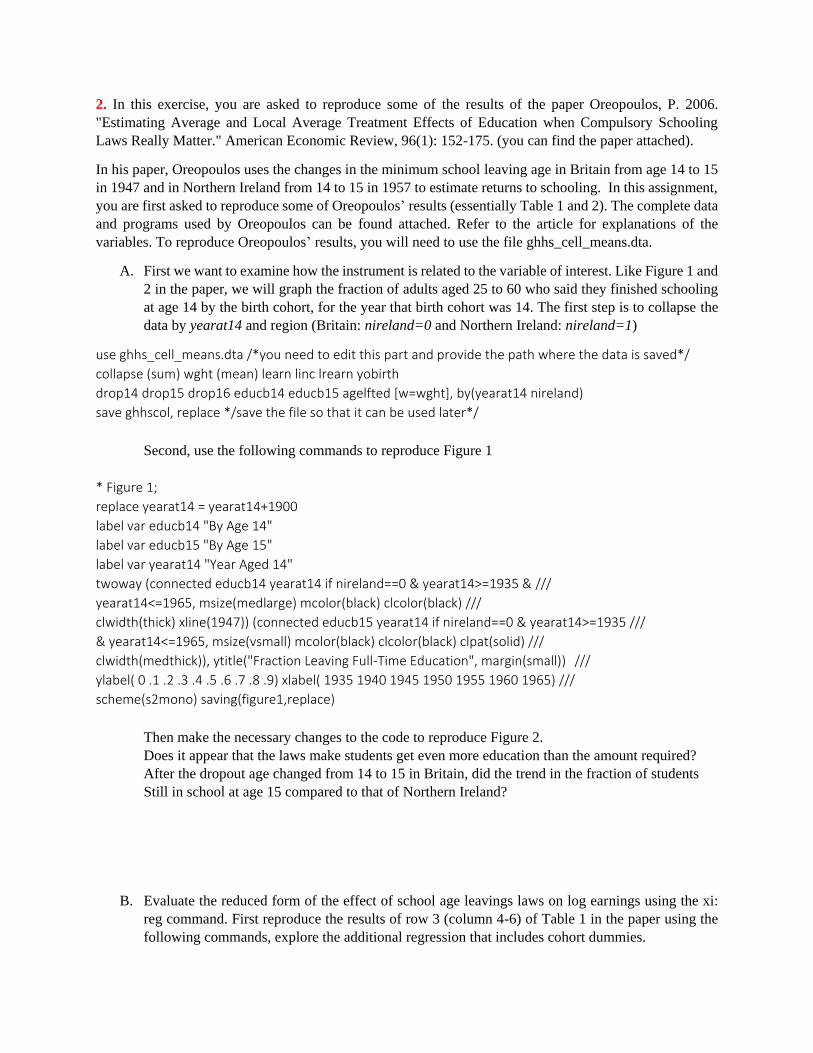
2. In this exercise, you are asked to reproduce some of the results of the paper Oreopoulos, P. 2006.

"Estimating Average and Local Average Treatment Effects of Education when Compulsory Schooling

Laws Really Matter." American Economic Review, 96(1): 152-175. (you can find the paper attached).

In his paper, Oreopoulos uses the changes in the minimum school leaving age in Britain from age 14 to 15

in 1947 and in Northern Ireland from 14 to 15 in 1957 to estimate returns to schooling. In this assignment,

you are first asked to reproduce some of Oreopoulos’ results (essentially Table 1 and 2). The complete data

and programs used by Oreopoulos can be found attached. Refer to the article for explanations of the

variables. To reproduce Oreopoulos’ results, you will need to use the file ghhs_cell_means.dta.

A. First we want to examine how the instrument is related to the variable of interest. Like Figure 1 and

2 in the paper, we will graph the fraction of adults aged 25 to 60 who said they finished schooling

at age 14 by the birth cohort, for the year that birth cohort was 14. The first step is to collapse the

data by yearat14 and region (Britain: nireland=0 and Northern Ireland: nireland=1)

use ghhs_cell_means.dta /*you need to edit this part and provide the path where the data is saved*/

collapse (sum) wght (mean) learn linc lrearn yobirth

drop14 drop15 drop16 educb14 educb15 agelfted [w=wght], by(yearat14 nireland)

save ghhscol, replace */save the file so that it can be used later*/

Second, use the following commands to reproduce Figure 1

* Figure 1;

replace yearat14 = yearat14+1900

label var educb14 "By Age 14"

label var educb15 "By Age 15"

label var yearat14 "Year Aged 14"

twoway (connected educb14 yearat14 if nireland==0 & yearat14>=1935 & ///

yearat14<=1965, msize(medlarge) mcolor(black) clcolor(black) ///

clwidth(thick) xline(1947)) (connected educb15 yearat14 if nireland==0 & yearat14>=1935 ///

& yearat14<=1965, msize(vsmall) mcolor(black) clcolor(black) clpat(solid) ///

clwidth(medthick)), ytitle("Fraction Leaving Full-Time Education", margin(small)) ///

ylabel( 0 .1 .2 .3 .4 .5 .6 .7 .8 .9) xlabel( 1935 1940 1945 1950 1955 1960 1965) ///

scheme(s2mono) saving(figure1,replace)

Then make the necessary changes to the code to reproduce Figure 2.

Does it appear that the laws make students get even more education than the amount required?

After the dropout age changed from 14 to 15 in Britain, did the trend in the fraction of students

Still in school at age 15 compared to that of Northern Ireland?

B. Evaluate the reduced form of the effect of school age leavings laws on log earnings using the xi:

reg command. First reproduce the results of row 3 (column 4-6) of Table 1 in the paper using the

following commands, explore the additional regression that includes cohort dummies.

se ghhs_cell_means.dta

gen age2 = age^2

gen age3 = age^3

gen age4 = age^4

gen yearat14_2 = yearat14^2

gen yearat14_3 = yearat14^3

gen yearat14_4 = yearat14^4

egen clust = group(yearat14 nireland)

xi: reg lrearn drop15 nireland yearat14 yearat14_2 yearat14_3 yearat14_4 [w=wght], cluster(clust)

xi: reg lrearn drop15 nireland yearat14 yearat14_2 yearat14_3 yearat14_4 age age2 age3 age4 ///

[w=wght], cluster(clust)

xi: reg lrearn drop15 nireland yearat14 yearat14_2 yearat14_3 yearat14_4 i.age [w=wght], cluster(clust)

xi: reg lrearn drop15 nireland i.yearat14 i.age [w=wght], cluster(clust)

Do your results match those of Oreopoulos? Try again using log nominal earnings learn instead of

log real earnings lrearn. What is the interpretation of the coefficient of drop15? Now modify the

above commands to reproduce row 1 and 2 (column 4-6). What is the problem in these cases with

the last regression that includes age and cohort dummies?

C. Replace drop15 by agelfted in (C) to obtain the OLS estimates of the returns to schooling. Can you

reproduce the results of columns 1-3 of Table 2? (Sometimes, the answer is no.) Are these estimates

likely to be biased, if yes in what direction?

D. Now estimate the first stage of the regression, that is the one that predicts schooling using dropout

laws. Here we will focus only on Britain and Northern Ireland together, but with a fixed effect for

Northern Ireland. First reproduce the results of row 3 (column 1-3) of Table 1 and obtain a

prediction of the education level (by the age left schooling) using the following commands:

xi: reg agelfted drop15 nireland yearat14 yearat14_2 yearat14_3 yearat14_4 [w=wght], cluster(clust)

predict pageled1

xi: reg agelfted drop15 nireland yearat14 yearat14_2 yearat14_3 yearat14_4 age ///

age2 age3 age4 [w=wght], cluster(clust)

predict pageled2

xi: reg agelfted drop15 nireland yearat14 yearat14_2 yearat14_3 yearat14_4 i.age ///

[w=wght], cluster(clust)

predict pageled3

Test whether the coefficient of drop15 is significant? Do we have a weak instrument? What is the

interpretation of this coefficient? Compare the goodness of fit with and without the drop15

variable? How important is this variable in predicting schooling?

E. Use the education prediction in (E) to estimate the second stage that is the effect of schooling on

earnings. Simply substitute pageled1 for drop15 in the first command in (C), pageled2 for drop15

in the second command in (C), and so on. What is your interpretation of the coefficient of pageled*?

Explain intuitively and briefly how you are estimating this coefficient, what is the source of

identification?

F. Use Stata’s ivreg command to perform the first and second stage of the estimation simultaneously.

What other changes do you have to make to reproduce the results of row 1 and row 3 (column 4-

6) of Table 2? Compare the coefficients and standard errors for agelfted with those of (F)? Which

is the correct one? Briefly explain.