Assignment 1: Investment Management

Student

Francesco Cardone

i7448606

Unit Tutor

Dr. Ishmael TINGBANI

18th March 2016

Introduction

This assignment demonstrates, through some computations, how a properly diversified portfolio reduces its

variability, which in this contest will be utilized as a measure of the risk of the portfolio. To meet these

requirements, five stocks have been chosen from an Index, “EURO STOXX 50”, which are: Unicredit (Italy,

Banking); Unilever (Netherland/UK, Food and Beverage); TOTAL (France, Petroleum); Volkswagen (Germany,

Automotive Industry); Allianz (Societas Europea, Munich, Insurance). All the shares have been selected to

represent different sectors, so as to enhance the differences and eventually obtain a better diversification.

The analysed data are daily prices adjusted for the dividends taken from a database (Datastream) concerning

the period October 1th 2015 - October 30th 2015.

Although the time period was limited, the choice of a month in which all the returns were positive presented a

more realistic idea of the long term behaviour that companies, such the “Blue Chips” mentioned above, should

(in theory) hold in the long run.

The choice of the EURO STOXX 50 Index (Europe's leading Blue-chip index for the Eurozone) was made

according to the international diversification principle that Reilly and Brown (2011, p.64) suggest: adding

foreign securities to a portfolio, i.e. creating a global portfolio, enables an investor to experience lower overall

risk since doing so the securities are not correlated with each other economies or stock market and this allows

for the elimination of some of the basic market risk of each individual country’s economy.

1) Presenting data: Average Return, Standard Deviation and

Covariance

Exhibit 1.1 shows the daily prices adjusted for the dividend for the month October 2015.

Exhibit 1.1

Source: Datastream

Exhibits 1.2 and 1.3 provide the percentage of returns for each period, the average returns, standard

deviations, variance and the covariance matrix.

Exhibit 1.2

Exhibit 1.3

In portfolio analysis, as described in Reilly and Brown (2011, p.175), a positive covariance means that the rates

of return for two stocks tend to move in the same direction relative to their individual means during the same

period. In contrast, a negative covariance indicates that the rates of return for two investments tends to move

in opposite directions. Therefore, aiming for diversification of the investment, to reduce the risk (which is

represented by the Variance and its square root, the Standard Deviation), investors tend to prefer a low or

negative Covariance.

2) Two stocks portfolio: combination Risk/Return and minimum

variance

Dividing the covariance between two stocks by their Standard Deviations, it is computed the correlation

coefficient (a standardized measure of the correlation) (Exhibit 2.1) which has the advantage to be comprised

between +1 and -1 ( −1 ≤ ϱ ≤ +1).

Exhibit 2.1

It is noticeable that the correlations Unicredit-Volkswagen and Unilever-Volkswagen are negative, so they will

provide a better portfolio diversification (the smaller -Unilever/Volkswagen- in particular). That is the reason

why they will be compared in this analysis. Exhibit 2.2 shows the combination of risk and return for the two

considered portfolios (Portfolio 1 and 2 respectively).

Exhibit 2.2

The most striking feature is how Portfolio 2 is dominant (better returns for the same level of risk).

Exhibit 2.3

Exhibit 2.3 presents (highlighted in red) the efficient part of the Portfolios, which for the same Risk offers a

better return. It is evident that for both the portfolios the efficient part of the curve starts at the point of

minimum variance, which can be calculated with the formula:

Xa =σb

2 − σaσbϱab

σa2 + σb

2 − 2σaσbϱab

𝑋𝑏 = 1 − 𝑋𝑎

where are used the SDs (σa,σb) of the two stocks and the correlation coefficient (ϱab).

In Exhibit 2.4 the combinations of risk and return for Portfolio’s (1 and 2) different weights are exposed in more

detail, highlighting in yellow how the Efficient Portfolio (for both 1 and 2) begins at the point of minimum

variance.

Exhibit 2.4

3) Five Stocks Portfolio

Analyzing different two-asset combinations and the curves which derive from assuming all the possible

weights, the result would be an envelope curve that contains the best of all these possible combinations: the

efficient frontier. Specifically, (Reilly and Brown, 2011, p.188) the efficient frontier represents that set of

portfolios that has the maximum rate of return for every given level of risk or the minimum risk for every level

of return. Therefore, if a portfolio is on the efficient frontier it dominates the others which are not.

In this analysis it has been considered an equally weighted portfolio just as one of the possible combinations.

Exhibit 3.1 Exhibi t 3.2

On Excel, it is possible to compute not only the equally weighted portfolio (Exhibit 3.1) but also, using Solver, a

combination which guarantees the minimum variance of the five stock portfolio (Exhibit 3.2). The constraints

on Solver are: minimizing the SD and the sum of the weight has to be 100%. (The weight of TOTAL is negative

so short selling is allowed).

It is noticeable how the equally weighted portfolio is dominated by the weight combinations that guarantee

the minimum variance point (in which the expected return is higher for a lower level of risk). It can also be seen

how the five stock equally weighted portfolio, in turn, dominates both Portfolio 1 and 2 (the two stocks

portfolios). (Exhibit 3.3)

Exhibit 3.3

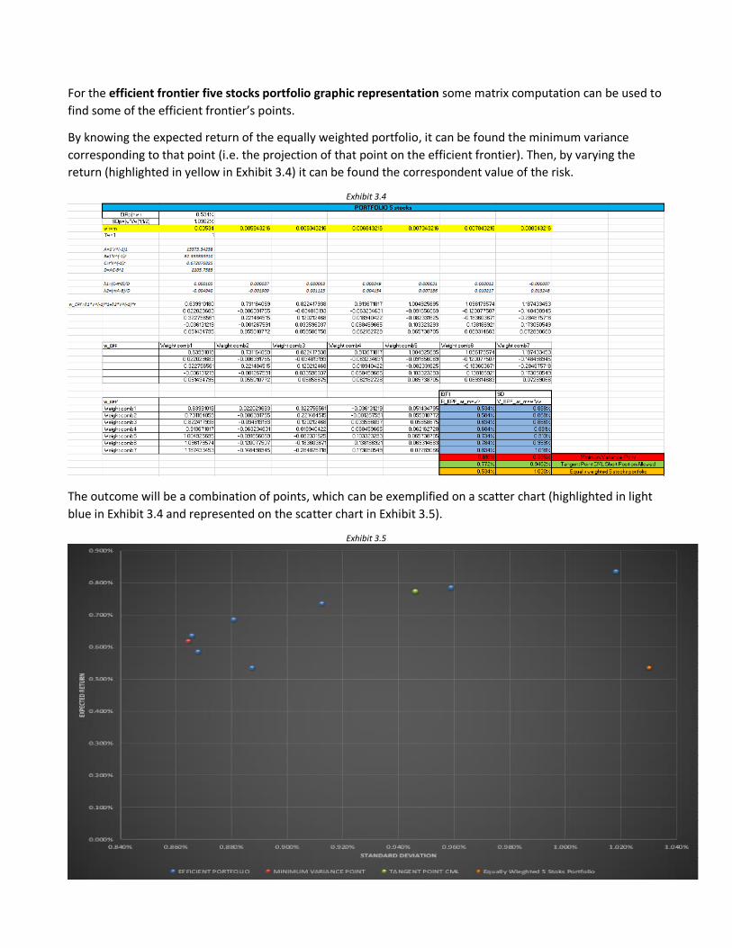
For the efficient frontier five stocks portfolio graphic representation some matrix computation can be used to

find some of the efficient frontier’s points.

By knowing the expected return of the equally weighted portfolio, it can be found the minimum variance

corresponding to that point (i.e. the projection of that point on the efficient frontier). Then, by varying the

return (highlighted in yellow in Exhibit 3.4) it can be found the correspondent value of the risk.

Exhibit 3.4

The outcome will be a combination of points, which can be exemplified on a scatter chart (highlighted in light

blue in Exhibit 3.4 and represented on the scatter chart in Exhibit 3.5).

Exhibit 3.5

Exhibit 3.5 also illustrates: the minimum variance point previously found with solver (highlighted in red); the

five stock equally weighted point (which can be compared with the first low point of our efficient frontier as

they have the same expected return but different weight and so a lower more efficient standard deviation);

and a point called tangent point CML (highlighted in green), which will be explained below.

Assuming that the five stocks portfolio includes all the risky assets in the market, it can be called market

portfolio. It contains all risky assets held anywhere in the marketplace and receives the highest level of

expected return per unit of risk for any available portfolio of risky assets. Under these conditions, drawing a

line, which includes not only the risky assets but also the risk free assets (hypothesis of lending and borrow at

the Risk Free Rate) the line is called Capital Market Line:

The CML equation is: E(Rport)= 𝑅𝐹𝑅 + σport[𝐸(𝑅𝑚)−𝑅𝐹𝑅

σM]

The slope of the CML is called Sharpe Ratio ([𝐸(𝑅𝑚) − 𝑅𝐹𝑅 σM⁄ ]), which is the maximum risk premium

compensation that investors can expect for each unit of the risk they bear (Reilly and Brown, 2011, p.198).

Thus, the investor will have four alternatives: investing in a market portfolio of risky assets; invest at the RFR;

invest partly in risky assets and partly in RFR; or borrow money at the RFR (leverage).

Trying to maximize the Sharpe Ratio with solver, under the constraint that the sum of the weight has to be

100%, with an approximate RFR of -0.175% considering the overnight Euro LIBOR interest rate for that period,

it will be found the point in which the CML is tangent to the efficient frontier.

Exhibit 3.6

The tangent point CML computed in Exhibit 3.6 and represented in Exhibit 3.5 (highlighted in green) is with

short position allowed. However, it can also be assumed that the weights do not have to be negative not

allowing a short position (the point so engendered will not be on the efficient frontier though).

4) Comment

All things considered, this work shows how to reduce the Standard Deviation of the total portfolio through

diversification, assuming imperfect correlations among securities. Moreover, it has been seen how adding

securities to a portfolio, which are not perfectly correlated with the stock already held, the overall standard

deviation of the portfolio can be reduced. At that point investors will have diversified away the unsystematic

risk, but not the market risk. Therefore, they cannot eliminate the variability and uncertainty of

macroeconomic factors that affect all risky assets (Reilly and Brown, 2011, p.202). Using securities coming from

different countries, i.e. creating a more global portfolio, and choosing different business sectors, it has tried to

underline how to eliminate some of the market risk.

To conclude, it can be appreciated, graphically, the difference in efficiency between a two stock portfolio

(Portfolio 2) and the more efficient five stock portfolio frontier (Exhibit 4.1), and the CML (Exhibit4.2).

Exhibit 4.1

Exhibit 4.2

REFERENCES

Datastream.

Reilly, Frank K. and Brown, Keith C. 2011. Analysis of Investment & Management of Portfolios. 10th edition.

Change Learning.