asset-liability management - booth school of...

© JRBirge INFORMS San Francisco, Nov. 2014 1

Asset-Liability Management

John Birge University of Chicago

Booth School of Business


Overview • Portfolio optimization involves:

• Modeling • Optimization • Estimation • Dynamics

• Key issues: • Representing utility (or risk and reward) • Choosing distribution classes (and parameters) • Building consistent models • Solving the resulting problems • Implementing solutions over time with non-stationary processes,

transaction costs, taxes, and uncertain future regulations

Outline

• Introduction • Modeling • Portfolio basics • Additions of assets and liabilities • Dynamics • Methods • Conclusion © JRBirge INFORMS San Francisco, Nov. 2014

Background on ALM • Manage a set of assets to meet a stream of

liabilities over time • Pension funds • Insurance companies • Banks

• Differences from standard portfolio optimization • Dynamics of liabilities/nonlinearities • State-dependent utility/contingencies

© JRBirge INFORMS San Francisco, Nov. 2014

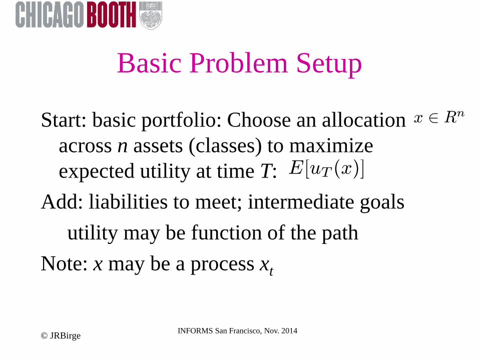
Basic Problem Setup

Start: basic portfolio: Choose an allocation across n assets (classes) to maximize expected utility at time T:

Add: liabilities to meet; intermediate goals utility may be function of the path Note: x may be a process xt


x 2 Rn

E[uT (x)]

Model


T

max E[) ut

(xt

)] t=1

s. t. xt+1

= rt

xt

+ bt

− st

− lt

,

(−τ +(b

t

) + τ−(s

t

) − lt

) = 0,

xt

∈ Nt

,

Model Construction


Asset returns: estimation issues, factor models, etc. to capture asset behavior

Liabilities: • Actuarial conditions • Losses due to claims • Losses to default • Relationships to asset trajectories (e.g., wages

to market return)

Example: bank model – rates for assets (loans), liabilities (deposits), losses (charge offs) (B., Judice)

Additional Issues

© JRBirge

Non-normal distributions (Chavez-Bedoya/B.): • Mean-variance may be far from optimizing utility • For exponential utility, can use generalized hyperbolic

distributions – closed form for some examples • Mean-variance can be close (but only if the risk-aversion

parameter is chose optimally)

Additional approaches: • Non-linear functions of Gaussian distributions • Can use polynomial approximations and higher moments to

obtain optimal solutions for these non-normal cases

Transaction Costs/Taxes and Dynamics

© JRBirge

Transaction costs:Each trade has some impact (e.g., bid-ask spread plus commission).Large trades may have long-term impacts.

Taxes:Taxes depend on the basis and vintage of an asset and involve alternative

selling strategies (LIFO, FIFO, lowest/highest price).

Quantstar 11

Why Model Dynamically? Three potential reasons:

Market timing Reduce transaction costs (taxes) over time Maximize wealth-dependent objectives

Example Suppose major goal is $100MM to pay pension liability in 2 years Start with $82MM; Invest in stock (annual vol=18.75%, annual exp.

Return=7.75%); bond (Treasury, annual vol=0; return=3%) Can we meet liability (without corporate contribution)? How likely is a surplus?

Quantstar 12

Alternatives

Markowitz (mean-variance) – Fixed Mix Pick a portfolio on the efficient frontier Maintain the ratio of stock to bonds to minimize expected

shortfall

Buy-and-hold (Minimize expected loss) Invest in stock and bonds and hold for 2 years

Dynamic (stochastic program) Allow trading before 2 years that might change the mix of

stock and bonds

Quantstar 13

Efficient Frontier

Some mix of risk-less and risky asset

For 2-year returns:

00.05

0.10.15

0.20.25

0.30.35

0.4

0 0.1 0.2 0.3 0.4

Quantstar 15

Best Dynamic Strategy

Start with 57% in stock If stocks go up in 1 year,

shift to 0% in bond If stocks go down in 1 year,

shift to 91% in stock Meet the liability 75% of

time

0

0.1

0.2

0.3

0.4

0.5

0.6

Stock Bond

0

0.2

0.4

0.6

0.8

1

1.2

Stock Bond0

0.10.20.30.40.50.60.70.80.9

1

Stock Bond

Stocks Up Stocks Down

Quantstar 16

Advantages of Dynamic Mix

Able to lock in gains Take on more risk when necessary to meet

targets Respond to individual utility that depends on

level of wealth

Target Shortfall

Approaches for Dynamic Portfolios Static extensions

Can re-solve (but hard to maintain consistent objective) Solutions can vary greatly Transaction costs difficult to include

Dynamic programming policies Approximation Restricted policies (optimal – feasible?) Portfolio replication (duration match)

General methods (stochastic programs) Can include wide variety Computational (and modeling) challenges

Basic Model with Transaction Costs

• Basic setup:

© JRBirge

Find x(t); b(t); s(t) to maximize E(u(x(T )) subject to x(0):

eTx+(t) = eTx(t)¡ ¿T b(t)¡ ¿T s(t);

eT (b(t) + s(t)) = 0;

x+(t) + (I + diag(¿))s(t)¡ (I ¡ diag(¿))b(t) = x(t);

where ¿ represents transaction costs and x(0) gives initial conditions and, with-out control, x(t) follows geometric Brownian motion dx(t) = x(t)(¹(t)+§(t)1=2dW (t))where W (t) represents n independent Brownian motions.

Continuous-Time Results Literature: Merton (1971), Magill and

Constantinides (1976), Davis and Norman (1990), Shreve and Soner (1994), Morton and Pliska (1995), Muthuraman and Kumar (2006), Goodman and Ostrov (2007)

Results: No trading in a region H; boundary at some distance from optimal no-transaction-cost point (for CRRA utility:

x*=(1/°)§-1(¹-r), Merton line) © JRBirge

General Result

© JRBirge

Time T

x1(t)

Merton line No-trade region

Equivalence in Discrete Time

© JRBirge

General observation: The continuous time solution is (approximately) equal to a discrete-time problem with a fixed boundary

Time T

x1(t)

Merton line No-trade region

T* Boundary here: same as for one period to T*.

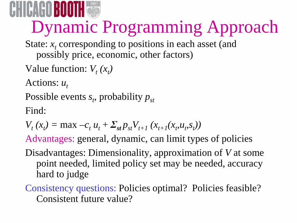
Dynamic Programming Approach State: xt corresponding to positions in each asset (and

possibly price, economic, other factors) Value function: Vt (xt) Actions: ut Possible events st, probability pst

Find: Vt (xt) = max –ct ut + Σst pstVt+1 (xt+1(xt,ut,st)) Advantages: general, dynamic, can limit types of policies Disadvantages: Dimensionality, approximation of V at some

point needed, limited policy set may be needed, accuracy hard to judge

Consistency questions: Policies optimal? Policies feasible? Consistent future value?

23

General Form in Discrete Time

Find x=(x1,x2,…,xT) and p (allows for “robust formulation”) to

minimize Ep [ ∑t=1Tft(xt,xt+1,p) ]

s.t. xt 2 Xt, xt nonanticipative, p2 P (distribution class) P[ ht (xt,xt+1,pt,) <= 0 ] >= a (chance constraint)

General Approaches: Simplify distribution (e.g., sample) and form a mathematical program:

• Solve step-by-step (dynamic program) • Solve as single large-scale optimization problem

Use iterative procedure of sampling and optimization steps

24

What about Continuous Time?

Sometimes very useful to develop overall structure of value function

May help to identify a policy that can be explored in discrete time (e.g., portfolio no-trade region)

Analysis can become complex for multiple state variables

Possible bounding results for discrete approximations (e.g., FEM approach)

Restricted Policy and ADP Approaches


Restricted Policy Approaches:

1. Fixed proportions

2. Fixed function of factors/state variables

3. Contingent functions

ADP Approaches:Approximate value function Vt(xt) by a combination of basis functions:

Vt(xt) =X

i

¸iÁi(xt)

and optimize over weights ¸.

26

Large-Scale Optimization Basic Framework: Stochastic Programming Model Formulation: Advantages:

General model, can handle transaction costs, include tax lots, etc.

Disadvantages: Size of model, insight

max Σσ p(σ) ( U(W( σ , T) ) s.t. (for all σ): Σk x(k,1, σ) = W(o) (initial) Σk r(k,t-1, σ) x(k,t-1, σ) - Σk x(k,t, σ) = 0 , all t >1; Σk r(k,T-1, σ) x(k,T-1, σ) - W( σ , T) = 0, (final); x(k,t, σ) >= 0, all k,t; Nonanticipativity: x(k,t, σ’) - x(k,t, σ) = 0 if σ’, σ ∈ St

i for all t, i, σ’, σ This says decision cannot depend on future.

27

Simplified Finite Sample Model Assume p is fixed and random variables represented

by sample ξit for t=1,2,..,T, i=1,…,Nt with

probabilities pit ,a(i) an ancestor of i, then model

becomes (no chance constraints): minimize Σt=1

T Σi=1Nt pi

t ft(xa(i)

t,xit+1, ξi

t) s.t. xi

t ∈ Xit

Observations? • Problems for different i are similar – solving one may help to solve others • Problems may decompose across i and across t yielding

• smaller problems (that may scale linearly in size) • opportunities for parallel computation.

Model Consistency Price dynamics may have inherent arbitrage

Example: model includes option in formulation that is not the present value of future values in model (in risk-neutral prob.)

Does not include all market securities available Policy inconsistency

May not have inherent arbitrage but inclusion of market instrument may create arbitrage opportunity

Skews results to follow policy constraints Lack of extreme cases

Limited set of policies may avoid extreme cases that drive solutions

Objective Consistency

Examples with non-coherent objectives Value-at-Risk Probability of beating benchmark

Coherent measures of risk Can lead to piecewise linear utility function forms Expected shortfall, downside risk, or conditional

value-at-risk (Uryasiev and Rockafellar)

Model and Method Difficulties

Model Difficulties Arbitrage in tree Loss of extreme cases Inconsistent utilities

Method Difficulties Deterministic incapable on large problems Stochastic methods have bias difficulties

Particularly for decomposition methods Discrete time approximations

Stopping rules and time hard to judge

Resolving Inconsistencies

Objective: Coherent measures (& good estimation) Model resolutions

Construction of no-arbitrage trees (e.g., Klaassen) Extreme cases (Generalized moment problems and fitting

with existing price observations)

Method resolutions Use structure for consistent bound estimates Decompose for efficient solution

Abridged Nested Decomposition (B., Donohue)

Incorporates sampling into the general framework of Nested Decomposition

Assumes relatively complete recourse and serial independence

Samples both the sub-problems to solve and the solutions to continue from in the forward pass through sample-path tree

Donohue/JRB 2006

Dual/Lagrangian-based Approaches

General idea: Relax nonanticipativity (or perhaps other constraints) Place in objective Separable problems

MIN E [ Σt=1T ft(xt,xt+1) ]

s.t. xt ∈ Xt xt nonanticipative

MIN E [ Σt=1T ft(xt,xt+1) ]

xt ∈ Xt + E[w,x] + r/2||x-x||2

Update: wt; Project: x into N - nonanticipative space as x

Convergence: Convex problems (Rockafellar and Wets); In portfolios (Haugh, Kogan, Wang/Brown, Smith Advantage: Maintain problem structure (e.g., network)


Summary Observations • Asset-Liability Management involves all of the

issues of dynamic portfolio optimization plus: • Modeling of the liability and asset relationships (not

simple linear forms) • Path-dependent utilities • Care to avoid arbitrage in model

• Solution methods involve some form of approximation • Price paths, Time/cost to no-trade • Discrete with value function, state, and path

decomposition • Dualization


Thank you!

asset-liability management - booth school of...

Documents