515

Assessment of Tractive Performances of Planetary Rovers with Flexible Wheels Operating in Loosely Packed Soils

J.P. Pruiksma*, J.A.M. Teunissen*, G..A.M. Kruse*, M.F.P. Van Winnendael**

*Deltares, Delft, The Netherlands e-mail: jitse.pruiksma@deltares.nl

**Automation and Robotics Section, European Space Agency e-mail: michel.van.winnendael@esa.int

Abstract

In view of project support work for ExoMars and possible subsequent Martian and Lunar ESA rover missions, a preliminary assessment has been made of the influence of a number of variables on wheel tractive performances on a loose fine sand, using state-of-the-art soil mechanics models and tools, i.e. the Abaqus Finite Element Method software with a Drucker-Prager Cap hardening 3-dimensional model mimicking a “Modified Cam-Clay Model” from Critical State Soil Mechanics. Especially for wheels with a deformable rim operating on loosely packed compressible soils this method of predicting tractive performances is expected to be more accurate than the currently existing semi-empirical models from classical terramechanics. For the currently baselined ExoMars Rover wheel design and a set of properties assumed for a fine sand which is expected to be representative for part of the Martian surface, the effects of wheel flexibility and wheel diameter on the tractive performances have been assessed, for a given load on the wheels and for a wide range of slip values. Moreover an assessment has been made, for this type of soil, of the effect of the gravity level on the load sinkage, within a range of wheel loads. This work can be considered a pilot project for exploring the possibilities of this method for future research and development.

1 Introduction

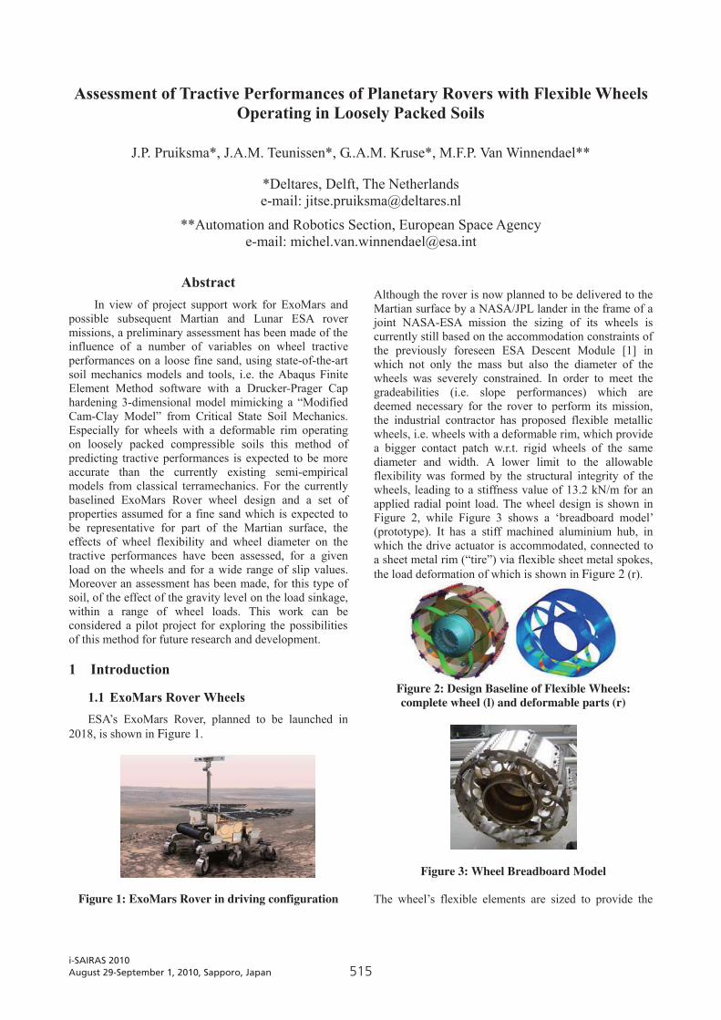
1.1 ExoMars Rover Wheels ESA’s ExoMars Rover, planned to be launched in

2018, is shown in Figure 1.

Figure 1: ExoMars Rover in driving configuration

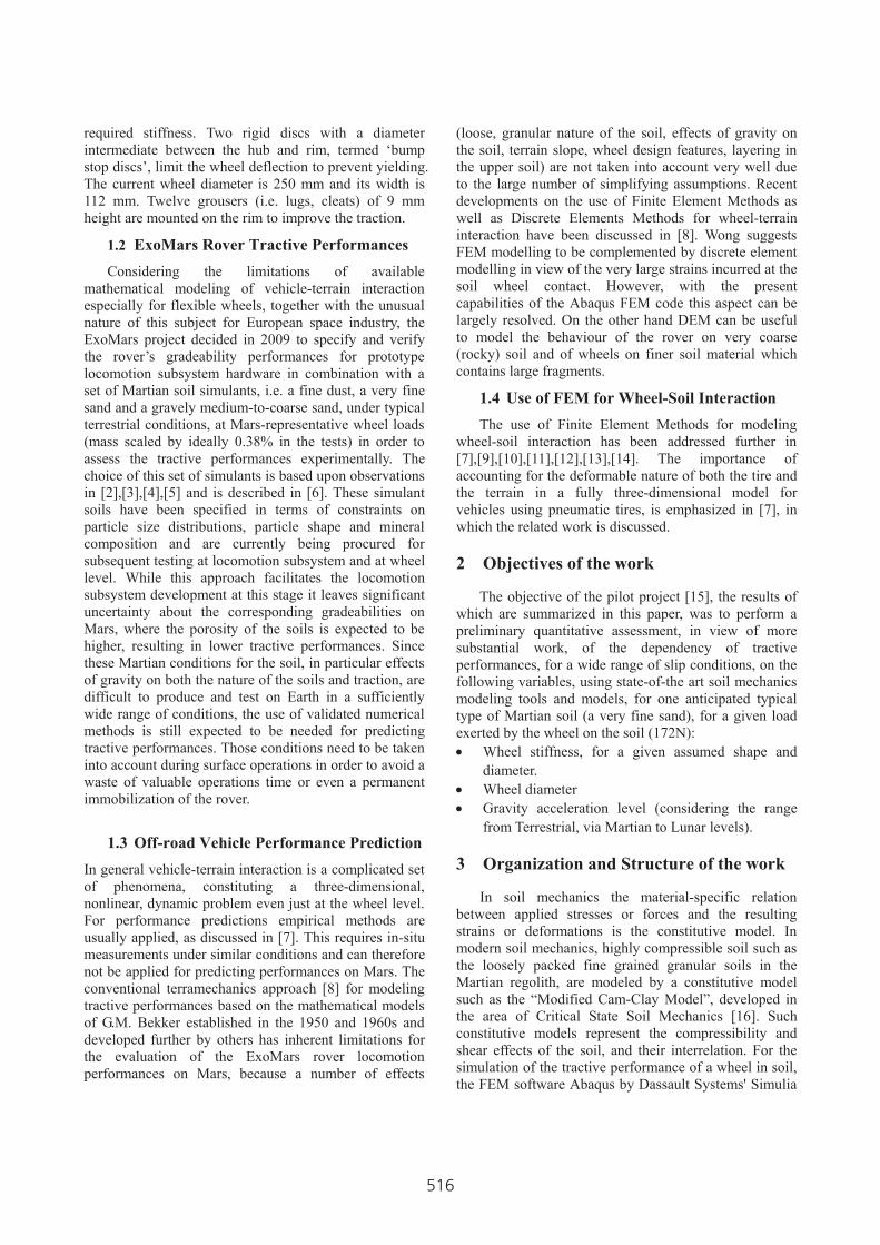
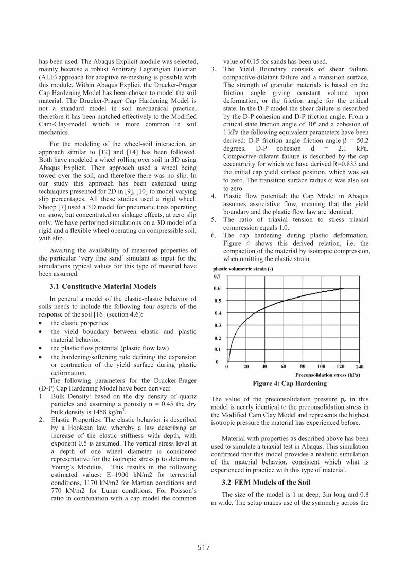
Although the rover is now planned to be delivered to the Martian surface by a NASA/JPL lander in the frame of a joint NASA-ESA mission the sizing of its wheels is currently still based on the accommodation constraints of the previously foreseen ESA Descent Module [1] in which not only the mass but also the diameter of the wheels was severely constrained. In order to meet the gradeabilities (i.e. slope performances) which are deemed necessary for the rover to perform its mission, the industrial contractor has proposed flexible metallic wheels, i.e. wheels with a deformable rim, which provide a bigger contact patch w.r.t. rigid wheels of the same diameter and width. A lower limit to the allowable flexibility was formed by the structural integrity of the wheels, leading to a stiffness value of 13.2 kN/m for an applied radial point load. The wheel design is shown in Figure 2, while Figure 3 shows a ‘breadboard model’ (prototype). It has a stiff machined aluminium hub, in which the drive actuator is accommodated, connected to a sheet metal rim (“tire”) via flexible sheet metal spokes, the load deformation of which is shown in Figure 2 (r).

Figure 2: Design Baseline of Flexible Wheels: complete wheel (l) and deformable parts (r)

Figure 3: Wheel Breadboard Model The wheel’s flexible elements are sized to provide the

i-SAIRAS 2010August 29-September 1, 2010, Sapporo, Japan

516

required stiffness. Two rigid discs with a diameter intermediate between the hub and rim, termed ‘bump stop discs’, limit the wheel deflection to prevent yielding. The current wheel diameter is 250 mm and its width is 112 mm. Twelve grousers (i.e. lugs, cleats) of 9 mm height are mounted on the rim to improve the traction.

1.2 ExoMars Rover Tractive PerformancesConsidering the limitations of available

mathematical modeling of vehicle-terrain interaction especially for flexible wheels, together with the unusual nature of this subject for European space industry, the ExoMars project decided in 2009 to specify and verify the rover’s gradeability performances for prototype locomotion subsystem hardware in combination with a set of Martian soil simulants, i.e. a fine dust, a very fine sand and a gravely medium-to-coarse sand, under typical terrestrial conditions, at Mars-representative wheel loads (mass scaled by ideally 0.38% in the tests) in order to assess the tractive performances experimentally. The choice of this set of simulants is based upon observations in [2],[3],[4],[5] and is described in [6]. These simulant soils have been specified in terms of constraints on particle size distributions, particle shape and mineral composition and are currently being procured for subsequent testing at locomotion subsystem and at wheel level. While this approach facilitates the locomotion subsystem development at this stage it leaves significant uncertainty about the corresponding gradeabilities on Mars, where the porosity of the soils is expected to be higher, resulting in lower tractive performances. Since these Martian conditions for the soil, in particular effects of gravity on both the nature of the soils and traction, are difficult to produce and test on Earth in a sufficiently wide range of conditions, the use of validated numerical methods is still expected to be needed for predicting tractive performances. Those conditions need to be taken into account during surface operations in order to avoid a waste of valuable operations time or even a permanent immobilization of the rover.

1.3 Off-road Vehicle Performance Prediction In general vehicle-terrain interaction is a complicated set of phenomena, constituting a three-dimensional, nonlinear, dynamic problem even just at the wheel level. For performance predictions empirical methods are usually applied, as discussed in [7]. This requires in-situ measurements under similar conditions and can therefore not be applied for predicting performances on Mars. The conventional terramechanics approach [8] for modeling tractive performances based on the mathematical models of G.M. Bekker established in the 1950 and 1960s and developed further by others has inherent limitations for the evaluation of the ExoMars rover locomotion performances on Mars, because a number of effects

(loose, granular nature of the soil, effects of gravity on the soil, terrain slope, wheel design features, layering in the upper soil) are not taken into account very well due to the large number of simplifying assumptions. Recent developments on the use of Finite Element Methods as well as Discrete Elements Methods for wheel-terrain interaction have been discussed in [8]. Wong suggests FEM modelling to be complemented by discrete element modelling in view of the very large strains incurred at the soil wheel contact. However, with the present capabilities of the Abaqus FEM code this aspect can be largely resolved. On the other hand DEM can be useful to model the behaviour of the rover on very coarse (rocky) soil and of wheels on finer soil material which contains large fragments.

1.4 Use of FEM for Wheel-Soil Interaction The use of Finite Element Methods for modeling

wheel-soil interaction has been addressed further in [7],[9],[10],[11],[12],[13],[14]. The importance of accounting for the deformable nature of both the tire and the terrain in a fully three-dimensional model for vehicles using pneumatic tires, is emphasized in [7], in which the related work is discussed.

2 Objectives of the work

The objective of the pilot project [15], the results of which are summarized in this paper, was to perform a preliminary quantitative assessment, in view of more substantial work, of the dependency of tractive performances, for a wide range of slip conditions, on the following variables, using state-of-the art soil mechanics modeling tools and models, for one anticipated typical type of Martian soil (a very fine sand), for a given load exerted by the wheel on the soil (172N):

Wheel stiffness, for a given assumed shape and diameter. Wheel diameter Gravity acceleration level (considering the range from Terrestrial, via Martian to Lunar levels).

3 Organization and Structure of the work

In soil mechanics the material-specific relation between applied stresses or forces and the resulting strains or deformations is the constitutive model. In modern soil mechanics, highly compressible soil such as the loosely packed fine grained granular soils in the Martian regolith, are modeled by a constitutive model such as the “Modified Cam-Clay Model”, developed in the area of Critical State Soil Mechanics [16]. Such constitutive models represent the compressibility and shear effects of the soil, and their interrelation. For the simulation of the tractive performance of a wheel in soil, the FEM software Abaqus by Dassault Systems' Simulia

517

has been used. The Abaqus Explicit module was selected, mainly because a robust Arbitrary Lagrangian Eulerian (ALE) approach for adaptive re-meshing is possible with this module. Within Abaqus Explicit the Drucker-Prager Cap Hardening Model has been chosen to model the soil material. The Drucker-Prager Cap Hardening Model is not a standard model in soil mechanical practice, therefore it has been matched effectively to the Modified Cam-Clay-model which is more common in soil mechanics.

For the modeling of the wheel-soil interaction, an approach similar to [12] and [14] has been followed. Both have modeled a wheel rolling over soil in 3D using Abaqus Explicit. Their approach used a wheel being towed over the soil, and therefore there was no slip. In our study this approach has been extended using techniques presented for 2D in [9], [10] to model varying slip percentages. All these studies used a rigid wheel. Shoop [7] used a 3D model for pneumatic tires operating on snow, but concentrated on sinkage effects, at zero slip only. We have performed simulations on a 3D model of a rigid and a flexible wheel operating on compressible soil, with slip.

Awaiting the availability of measured properties of the particular ‘very fine sand’ simulant as input for the simulations typical values for this type of material have been assumed.

3.1 Constitutive Material Models In general a model of the elastic-plastic behavior of

soils needs to include the following four aspects of the response of the soil [16] (section 4.6):

the elastic properties the yield boundary between elastic and plastic material behavior. the plastic flow potential (plastic flow law) the hardening/softening rule defining the expansion or contraction of the yield surface during plastic deformation. The following parameters for the Drucker-Prager

(D-P) Cap Hardening Model have been derived: 1. Bulk Density: based on the dry density of quartz

particles and assuming a porosity n = 0.45 the dry bulk density is 1458 kg/m3.

2. Elastic Properties: The elastic behavior is described by a Hookean law, whereby a law describing an increase of the elastic stiffness with depth, with exponent 0.5 is assumed. The vertical stress level at a depth of one wheel diameter is considered representative for the isotropic stress p to determine Young’s Modulus. This results in the following estimated values: E=1900 kN/m2 for terrestrial conditions, 1170 kN/m2 for Martian conditions and 770 kN/m2 for Lunar conditions. For Poisson’s ratio in combination with a cap model the common

value of 0.15 for sands has been used. 3. The Yield Boundary consists of shear failure,

compactive-dilatant failure and a transition surface. The strength of granular materials is based on the friction angle giving constant volume upon deformation, or the friction angle for the critical state. In the D-P model the shear failure is described by the D-P cohesion and D-P friction angle. From a critical state friction angle of 30º and a cohesion of 1 kPa the following equivalent parameters have been derived: D-P friction angle friction angle = 50.2 degrees, D-P cohesion d = 2.1 kPa. Compactive-dilatant failure is described by the cap eccentricity for which we have derived R=0.833 and the initial cap yield surface position, which was set to zero. The transition surface radius was also set to zero.

4. Plastic flow potential: the Cap Model in Abaqus assumes associative flow, meaning that the yield boundary and the plastic flow law are identical.

5. The ratio of triaxial tension to stress triaxial compression equals 1.0.

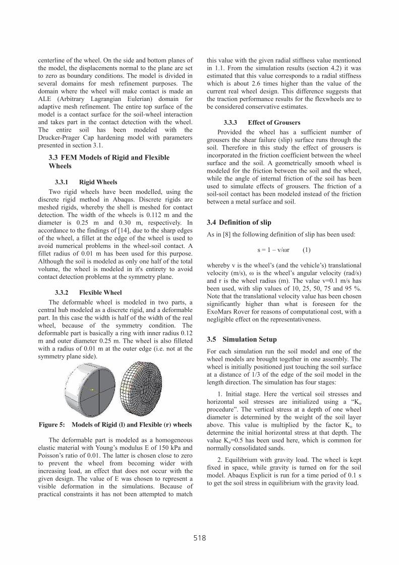
6. The cap hardening during plastic deformation. Figure 4 shows this derived relation, i.e. the compaction of the material by isotropic compression, when omitting the elastic strain.

Figure 4: Cap Hardening

The value of the preconsolidation pressure pc in this model is nearly identical to the preconsolidation stress in the Modified Cam Clay Model and represents the highest isotropic pressure the material has experienced before.

Material with properties as described above has been used to simulate a triaxial test in Abaqus. This simulation confirmed that this model provides a realistic simulation of the material behavior, consistent which what is experienced in practice with this type of material.

3.2 FEM Models of the Soil The size of the model is 1 m deep, 3m long and 0.8

m wide. The setup makes use of the symmetry across the

518

centerline of the wheel. On the side and bottom planes of the model, the displacements normal to the plane are set to zero as boundary conditions. The model is divided in several domains for mesh refinement purposes. The domain where the wheel will make contact is made an ALE (Arbitrary Lagrangian Eulerian) domain for adaptive mesh refinement. The entire top surface of the model is a contact surface for the soil-wheel interaction and takes part in the contact detection with the wheel. The entire soil has been modeled with the Drucker-Prager Cap hardening model with parameters presented in section 3.1.

3.3 FEM Models of Rigid and Flexible Wheels

3.3.1 Rigid Wheels Two rigid wheels have been modelled, using the

discrete rigid method in Abaqus. Discrete rigids are meshed rigids, whereby the shell is meshed for contact detection. The width of the wheels is 0.112 m and the diameter is 0.25 m and 0.30 m, respectively. In accordance to the findings of [14], due to the sharp edges of the wheel, a fillet at the edge of the wheel is used to avoid numerical problems in the wheel-soil contact. A fillet radius of 0.01 m has been used for this purpose. Although the soil is modeled as only one half of the total volume, the wheel is modeled in it's entirety to avoid contact detection problems at the symmetry plane.

3.3.2 Flexible Wheel The deformable wheel is modeled in two parts, a

central hub modeled as a discrete rigid, and a deformable part. In this case the width is half of the width of the real wheel, because of the symmetry condition. The deformable part is basically a ring with inner radius 0.12 m and outer diameter 0.25 m. The wheel is also filleted with a radius of 0.01 m at the outer edge (i.e. not at the symmetry plane side).

Figure 5: Models of Rigid (l) and Flexible (r) wheels The deformable part is modeled as a homogeneous

elastic material with Young’s modulus E of 150 kPa and Poisson’s ratio of 0.01. The latter is chosen close to zero to prevent the wheel from becoming wider with increasing load, an effect that does not occur with the given design. The value of E was chosen to represent a visible deformation in the simulations. Because of practical constraints it has not been attempted to match

this value with the given radial stiffness value mentioned in 1.1. From the simulation results (section 4.2) it was estimated that this value corresponds to a radial stiffness which is about 2.6 times higher than the value of the current real wheel design. This difference suggests that the traction performance results for the flexwheels are to be considered conservative estimates.

3.3.3 Effect of Grousers Provided the wheel has a sufficient number of

grousers the shear failure (slip) surface runs through the soil. Therefore in this study the effect of grousers is incorporated in the friction coefficient between the wheel surface and the soil. A geometrically smooth wheel is modeled for the friction between the soil and the wheel, while the angle of internal friction of the soil has been used to simulate effects of grousers. The friction of a soil-soil contact has been modeled instead of the friction between a metal surface and soil.

3.4 Definition of slip As in [8] the following definition of slip has been used:

s = 1 – v/ r (1)

whereby v is the wheel’s (and the vehicle’s) translational velocity (m/s), is the wheel’s angular velocity (rad/s) and r is the wheel radius (m). The value v=0.1 m/s has been used, with slip values of 10, 25, 50, 75 and 95 %. Note that the translational velocity value has been chosen significantly higher than what is foreseen for the ExoMars Rover for reasons of computational cost, with a negligible effect on the representativeness.

3.5 Simulation Setup For each simulation run the soil model and one of the wheel models are brought together in one assembly. The wheel is initially positioned just touching the soil surface at a distance of 1/3 of the edge of the soil model in the length direction. The simulation has four stages:

1. Initial stage. Here the vertical soil stresses and horizontal soil stresses are initialized using a “Ko procedure”. The vertical stress at a depth of one wheel diameter is determined by the weight of the soil layer above. This value is multiplied by the factor Ko to determine the initial horizontal stress at that depth. The value Ko=0.5 has been used here, which is common for normally consolidated sands.

2. Equilibrium with gravity load. The wheel is kept fixed in space, while gravity is turned on for the soil model. Abaqus Explicit is run for a time period of 0.1 s to get the soil stress in equilibrium with the gravity load.

519

3. Wheel indentation. The wheel is kept fixed horizontally and rotationally, while applying a vertical wheel load. The load is applied as a step function from 0 to 86 N (half of the ExoMars rover maximum wheel load of 172 kN at slope of 0 ). The load is increased in 10 steps and after each load has been applied it is kept constant for a period to arrive at a static solution for that load. The result of this stage is a sinkage versus load function for that particular wheel and soil.

4. Wheel Driving. The wheel load is kept constant at 86 kN, and the translational velocity v is ramped up linearly from zero to the nominal value in 0.1 s to have a smooth transition from stand still to motion. The rotation of the wheel without slip is kept free to simulate a wheel that is free-running. In the cases of nonzero slip, a rotational velocity of the wheel is applied according to eq. (1). This step is simulated for a time period of 6 s. This is enough to reach a steady state in most simulations.

The reaction force and torque on the wheel and its vertical displacement are the main output of the simulations, resulting in the graphs of sinkage, drawbar pull and input torque versus time. For the simulations of Terrestrial, Martian and Lunar conditions the gravity levels differ, as mentioned in chapter 2. For these conditions the initial soil stresses are different. This is taken into account. Also the elastic Young's modulus differs for which the values presented in section 3.1. The wheel load has been kept constant at 172 N in order to isolate the effect of gravity other than via variations of the wheel load.

Figure 6 visualizes the interaction for the flexwheel. The color scheme refers to the ‘PEEQ values’, i.e. the preconsolidation stress (in kPa).

3.6 Postprocessing The horizontal force (i.e. drawbar pull or net traction

at wheel level), input torque and vertical displacement of the wheel axle resulting from the simulations are saved at every time increment. This output is filtered and further processed to obtain the required results for the steady state wheel motion. Considering that the model represents only half of the wheel-soil interaction for reasons of model symmetry the drawbar pull and torque results are multiplied with a factor 2. A low pass filter at 10 Hz is used to ensure elimination of all aliasing effects. Nevertheless some oscillations are visible, also in the steady state results. Considering that the travel distance over which one oscillation takes place is about 0.033 m, which is approximately one element size, it can be concluded that the nature of the oscillations is related to mesh size.

Figure 6: Visualization of soil preconsolidation stress

in the flexwheel case

4 Results

4.1 Examples for Terrestrial Gravity Level Figure 7, Figure 8, and Figure 9 show the simulation

results for a rigid wheel under terrestrial conditions and 50% slip. Figure 7 shows the drawbar pull. During the wheel indentation stage up to 1.7 s the drawbar pull is approximately zero. After 1.7 seconds the driving stage of the simulation commences where the translational and angular velocities are increased to a constant value in about 0.1 seconds. Then the driving continues

Figure 7: DP for rigid wheel at 50 % slip

Figure 8: Input Torque for rigid wheel at 50 % slip

520

Figure 9: Sinkage for rigid wheel at 50% slip

until a steady state has been reached at approx. 5.5 seconds. From this time until the end of the simulation the average drawbar pull has been determined as this steady state and is later on compared with the results of the other simulations. Figure 8 shows similar result for the wheel input torque T, from which the tractive force (gross traction) can be calculated by dividing it by the wheel radius and the input power by multiplication by . Figure 9 shows the vertical displacement of the axle of the wheel, which in this case corresponds to the wheel sinkage, versus time. Up to 1.7 seconds the sinkage increases in small steps in response to the application of wheel load in ten equal load steps. Each time the load is increased quickly to the next level and then kept constant for the wheel to reach equilibrium. The end of the plateaus is the sinkage for that particular load. From these sinkages, a sinkage versus wheel load curve has been determined. Comparison of Figure 7, 8 and 9 shows that the start of wheel rotation results in temporary steep increase in sinkage and drop in drawbar pull, which recovers significantly after about 1.5 s, in about 1/5th rotation.

4.2 Main Results The results in Figure 10 and Figure 11 for a

deformable 0.25 m diameter wheel and the 2 sizes of rigid wheel (0.25 and 0.30 m diameter, respectively) show that a certain slip percentage is needed to create a positive drawbar pull. This is in line with observed experimental results for various soils and wheels and is consistent with the presence of compaction and bulldozing resistances as defined in [8]. Above about 50% slip both the drawbar pull and torque values reach a fairly constant value. The torque in the cases of the deformable and the rigid wheel of the same (0.25 m) diameter is almost equal, while the drawbar pull of the flexwheel is over 100 % higher. The drawbar pull for the larger 0.30 m diameter meter is about 50 % higher than for the smaller, 0.25 m dia, wheel and the required torque is 25 % higher. The differences in torque and drawbar pull between Terrestrial, Martian and Lunar conditions are small (at 50 % slip).

Figure 12 shows the sinkage versus wheel load during the indentation process. The sinkage is limited to about 4 cm. For the flexwheel both the vertical hub

displacement (labeled ‘wheel axle’) and sinkage (‘soil contact’) are shown. The larger diameter rigid wheel has less sinkage than the standard 0.25 m dia one. The sinkage of the rigid wheel is somewhat larger than for the flexwheel at the operational wheel load of 172 N, which is expected, due to the larger contact patch area. There is about 5 mm difference between hub displacement and sinkage, for the flexwheel at 172 N load, suggesting an equivalent stiffness of 34.4 kN/m, i.e. about 2.6 times higher than the corresponding value given in section 1.1.

Figure 10: DP vs slip for 2 sizes rigid and the

flexwheel

Figure 11: Input torque vs slip for 2 sizes rigid and

the flexwheel

Figure 12: Sinkage during indentation

Figure 13 leads to similar observation for the sinkage in steady state driving than for the indentation. In Figure 14 sinkage is shown for the rigid 0.25 m diameter wheel under Terrestrial, Martian and Lunar conditions in function of the wheel load. The differences are small, for the considered loads, which is in part related to the chosen soil properties. For significantly higher wheel

521

loads, the differences are expected to be bigger in that Lunar sinkages would be larger than the terrestrial ones for the same wheel load.

Figure 13: Sinkage in steady state driving

Figure 14: Sinkage vs. wheel load during indentation

at various gravity levels

5 Conclusions

In view of ExoMars and possible subsequent Martian and Lunar rover missions, a preliminary assessment has been made of the influence of a number of variables on wheel tractive performances on a loose fine granular soil, anticipated for Mars, using state-of-the-art soil mechanics models and tools, notably the Abaqus FEM software with a Drucker-Prager Cap Hardening Model. Studied variables are gravity level, wheel diameter and wheel stiffness. Simulations have been run for multiple levels of slip up to 95%. Soil compaction behaviour (load sinkage), torque and drawbar pull have been presented as simulation results. From the simulations following the conclusions can be drawn:

1. Soil mechanics model: It is possible to mimic very well advanced Critical State Soil Mechanics models with the Drucker-Prager Cap Model available in the Abaqus Explicit module.

2. Gravity level: Assuming a fixed wheel load the effect of gravity on the tractive performance and load sinkage is small, for the particular wheel load and soil type considered. Although the soil strength increases significantly faster with depth for terrestrial conditions compared to the Martian and Lunar conditions, this effect is not noticeable for the relatively small loads (and hence for the size of vehicle) considered here. The influence of the vehicle’s wheel reaches just the top few

decimeters of the soil, which for the chosen soil is determined mainly by the cohesion and not the internal friction angle, and is therefore largely independent of the stress level.

3. Wheel stiffness: The simulations for a flexwheel show a very significant, i.e. approx. 100 %, increase in drawbar pull compared to the rigid wheel of same diameter for slip values larger than 10 %, while the torque is lower for the flexwheel for a slip lower than 50 % and more or less equal to the torque for the rigid wheel above 50% slip. The results suggest that, for a flexwheel, less torque is needed to generate a higher drawbar pull. The sinkage for the deformable wheel is less than for the rigid wheel of same diameter, both for indentation at operational load and during the steady state in the rolling phase.

4. Wheel diameter: A 25 cm and 20 % larger (i.e. 30 cm) diameter wheel have been simulated. The larger diameter results in slightly decreased load sinkage, about 50 % higher drawbar pull, and about 25 % increased torque compared to the smaller diameter wheel.

5. Tractive performance: The drawbar pull and torque generally increase with increasing slip. For a slip over 50% there is no significant change in drawbar pull and torque, however. At a low slip (smaller than approx. 3%) the drawbar pull is negative due to the sum of compaction and bulldozing resistances.

6 Recommendations for further work

Despite the very promising results of this pilot project a lot of additional work should be undertaken in order to obtain a validated tool that can be used to predict locomotion performances of a planetary or lunar rover. In particular the following points can be mentioned:

Effect of soil parameter values. The simulation results are sensitive to the soil cohesion and compaction behaviour in the range anticipated in studies on properties of Martian regolith. Further study is recommended of the effect of these variables in view of the larger differences between Terrestrial, Martian and Lunar conditions found in experiments under reduced gravity levels than found in the simulations in this report. The difference in findings may be due to the cohesion and compaction properties assumed.

Validation of simulations by comparison with experimental results: instead of assuming soil parameter values, measured soil properties shall be used as inputs for the simulations, and the outputs

522

shall be compared with results from single wheel testbed measurements.

Effects of the width of wheels including trade-off of diameter increase versus width increase for improving traction. This could become very relevant in case the upcoming tests would lead to the conclusion that the currently baselined ExoMars Rover wheels are too small. Performing this tradeoff by hardware trial and error is expected to be significantly more costly than by this method.

Assessment of a wider range of flexibility (stiffness) and wheel diameter values.

Study of vehicles of larger mass and wheel loads. In this case larger differences in tractive performance between Terrestrial and Martian conditions are expected than found in the presented study based on the ExoMars wheel design and wheel load. This is related to the sensitivity for effects of cohesion and compaction of the soil.

Soil with more layers. This is relevant for study of for example the effect of a crust on Martian soils, and presence of a hard substratum for loose soil.

Effect of inclination of the terrain on the tractive performance. The inclination is expected to affect the bulldozing resistance.

Explicit calculation of the tractive force and wheel-external motion resistances (due to compaction and bulldozing effects), both in case of rigid and flexible wheels.

Acknowledgment The work presented was performed by Deltares in the frame of a Technical Assistance activity funded by ESA’s Technical Directorate, based on wheel design information provided by the ExoMars industrial team. References [1] M. Van Winnendael, P. Baglioni, A. Elfving, F.

Ravera, J. Clemmet, E. Re, “ The ExoMars Rover – Overview of Phase B1 Results”, 9th International Symposium on Artificial Intelligence, Robotics and Automation in Space, iSairas 2008, Los Angeles, 26-29 Feb. 2008.

[2] Arvidson, R.E., J.L. Gooding and H.J. Moore, “The Martian surface as imaged, sampled and analyzed by the Viking landers”, Reviews of Geophysics, 27/1, 1989, pp. 39-60.

[3] Herkenhoff, K.E., M.P. Golombek, E.A. Guinness, J.B. Johnson, A. Kusack, S. Gorevan, L. Richter, and R.J. Sullivan, “In situ observations of the physical properties of the Martian surface”, in: J.

Bell (ed.) The Martian Surface: Composition, mineralogy, and physical properties. Cambridge Un. Press, Cambridge, 2008, pp 451-467.

[4] Moore, H.J., R.E. Hutton, R.F. Scott, C.R. Spitzer, and R.W. Shorthill, “Surface materials of the Viking Landing sites”, Journ. Geoph. Res., 1977, 82/28, pp. 4497-4523.

[5] Moore, H.J. and G..D. Clow “A summary of Viking sample-trench analyses for angles of internal friction and cohesions”, Journ. Geoph. Res., 1982, 87/B12, pp. 10,043-10,050.

[6] G. Kruse, Reference Soils for Locomotion Tests of the ExoMars Rover – A Brief Review, Deltares Report Ref. 1200662-000-GEO-0003, Rev. 1, 15 July 2009, commissioned by ESA.

[7] S. A. Shoop, “Finite Element Modeling of Tire–Terrain Interaction”, US Army Corps of Engineers, Engineer Research and Development Center, Report ERDC/CRREL TR-01-16, 2001.

[8] Wong, J.Y., Theory of Ground Vehicles, Wiley, 2008.

[9] C.H. Liu, J.Y. Wong, “Numerical simulations of tire-soil interaction based on critical state soil mechanics”, Journal of Terramechanics, 1996, vol 33, no 5, pp. 209-221.

[10] C.H. Liu, J.Y. Wong, H.A. Mang, “Large strain finite element analysis of sand: model, algorithm and application to numerical simulation of tire-sand interaction”, Computers and Structures, 74 (2000), pp. 253-265.

[11] C.W. Fervers, “Improved FEM simulation model for tire-soil interaction”, Journal of Terramechanics 41 (2004) 87-100.

[12] R. C. Chiroux, W. A. Foster Jr., C. E. Johnson, S. A. Shoop, R. L. Raper, “Three-dimensional finite element analysis of soil interaction with a rigid wheel”, Applied Mathematics and Computation, Volume 162, Issue 2, 15 March 2005, pp. 707-722, ISSN 0096-3003, DOI: 10.1016/j.amc.2004.01.013.

[13] J.P. Hambleton, A. Drescher, “Modeling wheel-induced rutting in soils: Indentation”, Journal of Terramechanics 45 (2008), pp. 201-211

[14] J.P. Hambleton, A. Drescher “Modeling wheel-induced rutting in soils: Rolling”, Journal of Terramechanics 46 (2009), pp. 35-47.

[15] J.P. Pruiksma, J.A.M. Teunissen, Preliminary Numerical Assessment of Tractive Performances of Rover Wheels, Deltares Report Ref. 1201417-000-GEO-0004-sr, Jan. 2010, commissioned by ESA.

[16] Wood, D.M., Soil Behaviour and Critical State Soil Mechanics, Cambridge University Press2007 (first published 1990).