assessment of the evolution equation modelling approach for three-dimensional expanding wrinkled...

Combustion and Flame 159 (2012) 1932–1948

Contents lists available at SciVerse ScienceDirect

Combustion and Flame

journal homepage: www.elsevier .com/locate /combustflame

Assessment of the Evolution Equation Modelling approach forthree-dimensional expanding wrinkled premixed flames

Eric Albin, Yves D’Angelo ⇑CORIA/INSA UMR 6614 CNRS, Avenue de l’Université 76801, Saint-Etienne du Rouvray, Rouen, France

a r t i c l e i n f o a b s t r a c t

Article history:Received 23 September 2011Received in revised form 27 September2011Accepted 27 December 2011Available online 26 January 2012

Keywords:Expanding premixed flamesEvolution Equation ModellingDirect Numerical Simulation

0010-2180/$ - see front matter � 2012 The Combustdoi:10.1016/j.combustflame.2011.12.019

⇑ Corresponding author.E-mail address: [email protected] (Y. D’Angelo).

Direct Numerical Simulations (DNS), Evolution Equation Modelling (EEM) and Experimental results fromthe literature (EXP) are presented and analyzed for an expanding propane/air flame. DNS results areobtained thanks to the in-house finite-difference code HAllegro. Computed (DNS/EEM) and measured(EXP) equivalent radii RP and RS, mean stretch k and consumption velocity SC, as well as sample frontshapes, are compared using the same post-processing procedure. Small perturbations in the EEM inputparameters induce comparatively small shifts in the compared results, showing the robustness of theapproach. When slightly adapting only one Oð1Þ parameter for the EEM strategy (the effective turbulentforcing amplitude felt by the flame), DNS, EEM and EXP show quite fair agreement one another, except forone of the experiments at early times. In the context of expanding flames, this validated EEM methodol-ogy can constitute a reliable tool to compute realistically large sized flames.

� 2012 The Combustion Institute. Published by Elsevier Inc. All rights reserved.

1. Introduction

Expanding flames constitute a basic fundamental configurationfor pre-mixed laminar and turbulent gaseous combustion. Theyhave been (and are still) extensively studied under varying condi-tions (pressure, temperature, fuel, Lewis number . . . ) both experi-mentally and numerically, for instance to determine laminar flamevelocities and/or Markstein lengths (see e.g. [1,2]).

In many practical applications, turbulent pre-mixed flames canbe considered as a collection of locally laminar flames: the flameletregime [3], where turbulence does not substantially modifies theinternal structure of the laminar flame. Furthermore, for suffi-ciently moderate turbulence, the flame is only wrinkled and theturbulent expanding flame front can be considered as a slightly de-formed (‘‘wrinkled’’ or ‘‘corrugated’’) sphere.

In [4], turbulent 3D expanding air/methane, air/propane andair/hydrogen flames are measured at atmospheric pressure. Aninternal combustion engine-like configuration, with an opticallyaccessible cylindrical combustion chamber has also been consid-ered in [5–7]. Ref. [8] (results from [8] will also be compared withthose of present paper) is interested in the dynamics of an expand-ing propane/air flame, again in an engine-like configuration.

To investigate the expanding flame behaviour, one can numer-ically solve the full set of 3D Navier–Stokes reactive equations (seefor instance [9–11] or the recent work [12]). However, for realisti-cally large sizes, and because of the very small spatio-temporal

ion Institute. Published by Elsevier

scales involved both from turbulence and chemical reaction, therequired computational effort may become impractical, in particu-lar if one tries to reach the regime where the expanding flameaccelerates [13,14].

Instead of using ‘‘brute force’’ simulations, one can try instead totake advantage of the scale separation (the flame front is very thin)and solve an evolution equation for the flame front only. Since onlythe flame surface needs to be parameterized, one spatial dimensionis removed from the computation. Moreover, all pertinent physicalparameters can be lumped into a reduced set; here, as this will bespecified on the sequel, only three (plus one) physical parametersare needed: namely the density contrast a, the Markstein lengthLu and the laminar flame velocity S0

L . To mimic turbulent flow, andsince the Evolution Equation Modelling (EEM) approach does notsolve for the flow, a synthetic turbulent forcing u0 must also be sup-plied. The aim of the paper is to tentatively assess a chosen EEMstrategy for 3D expanding flames (from Ref. [15]) by comparing itsresults with present Direct Numerical Simulations (DNS) and avail-able experimental data from the literature.

For the DNS calculations, we used the in-house compressiblecode HAllegro while experimental results are those of [4,8]. Theseexperiments were considered because (i) we are mainly interestedon the effect of weak (u0/SL � 1) turbulence on the flame; (ii) theconfiguration is quite straightforward to compute (an expandingstoichiometric propane/air flame at room pressure); (iii) we haveaccess to the experimental data and we can use the same post-pro-cessing strategy for our DNS results.

The paper is organized as follows. Basic definitions of the set-upand of experimental outputs, i.e. the profiles of quantities that will

Inc. All rights reserved.

http://dx.doi.org/10.1016/j.combustflame.2011.12.019

mailto:[email protected]

http://dx.doi.org/10.1016/j.combustflame.2011.12.019

http://www.sciencedirect.com/science/journal/00102180

http://www.elsevier.com/locate/combustflame

E. Albin, Y. D’Angelo / Combustion and Flame 159 (2012) 1932–1948 1933

be actually compared to the DNS and EEM computations, are intro-duced in Section 2. Section 3 presents the system of governingequations solved by the in-house code HAllegro. The DNS andEXP post-processing procedure, based on polynomial interpolation[4], and its limitations, as well as the influence of BC treatment onthe shape of the computed flame, are also tested on preliminarylaminar benchmarks. The numerical set-up for turbulent wrinkledflames computation is finally presented at the end of the section.The EEM approach, similar to the one from [15], is outlined in Sec-tion 4, as well as the adopted numerical strategy (Exponential TimeDifferencing Runge–Kutta method, or ETDRK, in the Fourier–Legendre basis) to solve it. The way to mimic external ‘‘turbulent’’forcing by a Passot–Pouquet spectrum and a proposed equation forthe mean flame radius can also be found there.

Section 5 shows comparisons and analysis of DNS/EEM/EXP re-sults. Also included is robustness testing of the EEM strategy whenslightly varying some input parameters. Concluding remarks andperspectives end the paper in Section 6.

2. Basic definitions, Markstein law

In this section, we introduce the basic quantities that are exper-imentally determined and that will be used as comparison fornumerical modelling (DNS and EEM).

2.1. Basic definitions, general case

A three-dimensional spherical flame can be triggered by sparkelectrodes in a turbulent pre-mixture of e.g. air/propane. Experi-mental techniques such as PIV and laser tomography may thengive access to pictures of flame surface and burnt gas production.

If the flame front is sufficiently thin, and separates burnt gas(refered to with b subscript in the sequel) from fresh (unburned)mixture (refered to with u subscript), two experimentally accessi-ble characteristic radii, respectively denoted RS and RP can be intro-duced. They are based on burnt gas surface S (Eq. (1a)) and two-dimensional flame section perimeter L (Eq. (1b)):

S ¼ pR2S ð1aÞ

L ¼ 2pRP ð1bÞ

Figure 1 presents a typical sample contour of experimentallyobtained flame surface contour. From a measured image, radiusRS can be determined by computing the number of pixels associ-ated with burnt gas. For RP, it is necessary to evaluate the flamelength. One should first determine which pixels belong to theflame front, then smooth the contour before evaluating its length

Rs Rp

S

L

Fig. 1. Experimentally determined equivalent flame radii RS and RP; Eqs. (1a) and(1b).

[4]. These two radii can be related to consumption speed SC, meanturbulent flame velocity ST (the mean displacement speed) andmean stretch k, that will be defined below.

For a cylindrical-in-average or spherical-in-average turbulentflame, the mean turbulent velocity ST can be computed as [4,16,1]

ST ¼qb

qu

dRS

dt¼ ð1� aÞdRS

dtð2Þ

where a denotes the density contrast a ¼ qu�qbqu

. Eq. (2) can be ob-tained by mass conservation through the (infinitely thin) flamefront. The consumption rate of the fresh mixture SC (the mean burn-ing velocity) can similarly be expressed as

SC ¼qb

qu

RS

RP

� �n dRS

dtð3Þ

with n = 1 for cylindrical-in-average flames and n = 2 for spherical-in-average flames. Note that Eq. (3) assumes that the front is infi-nitely thin. If a non-zero (thermal) thickness lt is assumed for the3D front (i.e. if lt/RP is not �1), another expression can be derivedfor SC [17,18]

SC ¼qb

qu

RS

RP

� �2 dRS

dt1

1þ ðlt=RPÞ2

!ð4Þ

The local flame stretch j can be defined as [19,4,18]

j � 1dS

@dS@t

ð5Þ

where dS is a local element of front surface. From Eq. (5), one candeduce the mean flame stretch k as [20]

k ¼ 1Su

dSu

dtð6Þ

with Su the total flame front surface. It is linked to RP according to[17,18]

k ¼ nRP

dRP

dtð7Þ

with again n = 1 for cylindrical-in-average flames and n = 2 forspherical-in-average flames.

From asymptotic theory and experiments, the consumption rateSC can be related to mean flame stretch k according to [17,19,18]

SC ¼ S0L � Luk ð8Þ

where Lu is a Markstein length and S0L is the laminar (unstretched)

flame velocity.

2.2. Laminar case

In the laminar case, for 2D and 3D expanding flames, the front isperfectly circular or spherical. Hence, the above introduced radiiare identical: RS = RP = R and the stretch k (mean or local) is equalto k ¼ n

RdRdt . Markstein law (8) becomes

dRdt¼ S0

L

1� a� Lb

nR

dRdt

ð9Þ

where Lb ¼ Lu=ð1� aÞ denotes the ‘‘second Markstein length’’ [19].Eq. (9) can finally be cast as

dRdt¼ S0

L

1� a� 11þ nLb=R

: ð10Þ

This equation admits a closed form solution — the Lambert functionof an exponential [21] — or may be more conveniently solvednumerically. These analytical results as well as experiments from

1934 E. Albin, Y. D’Angelo / Combustion and Flame 159 (2012) 1932–1948

[8] will be used to validate preliminary DNS results for the laminarcase, as it will be shown in Section 5.

3. DNS of expanding flames

3.1. Governing equations, numerical strategy, BCs

The set of governing equations are the fully compressible reac-tive Navier–Stokes equations, that can be cast as

� @q@t¼ @qUj

@xjð11Þ

� @qUi

@t¼ @qUiUj

@xjþ @P@xi� @sij

@xjð12Þ

� @qE@t¼ @

@xjðUjðP þ qEÞÞ � @

@xjk@T@xj

� �� @sijUi

@xj� eS5 ð13Þ

� @qYk

@t¼ @qUjYk

@xj� @

@xjD@Yk

@xj

� �� eSk ð14Þ

in conservative form and with usual notations. Temperature T is de-duced from total energy qE = qCVT + q Ui

2/2. (Notice that specificheat capacity CV is assumed constant.) Pressure is computed fromperfect gas law P = qrT and power law is assumed for dynamic vis-cosity l � T0.76. Heat diffusion coefficient k and scalar conductivityD are deduced from dynamic viscosity l by assuming fixed values ofPrandtl (Pr = 0.795) and Schmidt (Sc = 1.113) numbers, yielding aLewis number of 1.4 for stoichiometric propane/air. The stress ten-sor sij is given by its Newtonian fluid expression (with dij the Kro-

necker delta): sij ¼ l @Ui@xjþ @Uj

@xi

� �� 2

3 l@Uk@xk

dij. The terms eSk and eS5

represent source terms due to combustion. Chemistry is simplifiedassuming single step Arrhenius kinetics; pre-exponential factor istuned with respect to local equivalence ratio in order to fit the cor-rect value of the laminar flame velocity [22].

The DNS solver we employed is the in-house parallel solverHAllegro [23,24]. It is based on a 6th-order compact explicit finitedifference scheme, applied on hybrid collocated/staggered grids,coupled to a low-storage third-order Runge–Kutta algorithm tomarch in time. Within the context of the present work, the mainadvantages of the solver are (i) increased robustness, comparedwith a pure collocated strategy, i.e. the possibility of using coarsergrids while preserving the same accuracy; (ii) the unambiguousdefinition of boundary points, compared with a pure staggeredstrategy, allowing for straightforward acoustic outflow BC treat-ment. For the expanding flames we computed, non reflecting out-flow treatment of [25] demonstrated robustness and very lowinfluence on flame shape, while the non-reflecting strategy of[26] makes the flame become square, as will be shown Fig. 3a.

3.2. Laminar case, post-processing

To ensure a coherent comparison between numerical andexperimental results, we made use of the same post-processingprocedure — in particular the same interpolation (smoothing) pro-cedure for determining the flame front — as the one used in [4,17].We shall discuss in this subsection some experimental and numer-ical shortcomings: on the one hand, the post-processing interpola-tion procedure does not allow to correctly capture the flame frontunder a 2 mm radius; on the other hand, the numerical boundarycondition treatment (the popular NSCBC and 3D-NSCBC) may in-duce a square-shaped front when approaching the outflowboundaries.

We hence tested the procedure on laminar flames, both forcylindrical and spherical fronts. We performed three computa-tions: (i) a cylindrical flame with usual NSCBC outlets [26], (ii) acylindrical flame with 3DNSCBC outlets [25,27], (iii) a spherical3D flame with 3DNSCBC. Since we would like to test the presentprocedure mainly for the turbulent case, we do not exploit anysymmetries in the computations. The mixture is ignited by forcingat initial time a Gaussian profile for temperature and compositionat the center of the computational domain.

Figure 2 represents temperature contours for each of thesethree cases. The points (� pixels, for a corresponding measure-ment) where T (in Kelvins) stands in the interval [1076;1223]are reproduced as +. The used smoothing procedure [4] consistsin polynomial interpolation to determine the RP radius.

At initial time t = 0, Fig. 2 shows a significant discrepancy be-tween the simulated front and the smoothed front. At small radii,the flame front is not sufficiently resolved (too few points/pixelsto mark it) and it seems that at these early times the smoothingprocedure is not able to find a suitable front shape and position.At larger times and radii, the resolution is sufficient and the valueof RP reliable. From these preliminary results, and as in the exper-iments [4], we considered that the front shape and position wascorrectly captured by the smoothing procedure only above a radiusvalue of 2 mm.

Figure 3 presents ten equally spaced (in time) contours for thethree aforementioned configurations. For cylindrical flames, theflame radius increases at a constant rate as shown in Fig. 3b. Inthe spherical case, Fig. 3c shows that the flame speed tends to in-crease with time.

Figure 4 shows flame radius time evolution R(t) for propane/airlaminar flames in the 2D and 3D expanding cases. As expected, inthis laminar case, the two computed radii RS and RP were foundnumerically equal to R. For the three computational cases (2D withNSCBC or 3DNSCBC, 3D with 3DNSCBC), we plot the computed ra-dius against experimental results from [4,8]. From Eqs. (2), (3) and(7), we can compute consumption velocity SC, mean velocity ST andstretch k. Evolutions for SC, ST and k as a function of R(�RS � RP) areshown in Figs. 5 and 6. Since radius is almost linear in time (seeFig. 4), their temporal evolutions present very similar profiles tothose of Figs. 5 and 6. They are not presented here. Figure 7 showsconsumption velocity SC as a function of k. Again, all these com-puted quantities are compared with experimental results from[4,8].

As expected [4], flame radius increases faster in the cylindricalconfiguration and the influence of boundary condition treatmentremains small. In the cylindrical case, the flame consumptionvelocity tends quite quickly to its limit (planar) valueS0

L ¼ 0:407 m=s, while in the spherical case SC stays at a lesser levelduring the evolution, as also noticed experimentally in [4,8].

Very good agreement is obtained between DNS results of thespherical case and experimental results from [8], as is the observedtrend for larger radii. However, results from [4], even if compatibleat large times/radii, do not match neither DNS nor results from [8].Estimation of SC or k is very sensitive to the smoothing procedureused to compute dR/dt from raw data [21] and also to measure-ment frequency. This may be the main cause of the observed dis-crepancies. Another possible source of inaccuracy at early timesmay rely in the ignition device of the experimental configuration.In [4], the convected flow is ignited by two electrodes that maygive a bean-shaped profile for the ignition kernel. In [8], the ignitedflow is steady and we may think the initial kernel remains morespherical.

Figure 7 shows that consumption velocity is a linear function ofstretch k. However, a short transient is observed before Marksteinlaw is verified (cf. large values of k, i.e. small values of radius ortime). This may be due to our Gaussian initialization procedure

y (c

m)

−0.04

−0.02

0

0.02

0.04

0.06

−0.06−0.04−0.02 0 0.02 0.04 0.06

resultsource

x (cm)

−0.06

result

−0.04

−0.02

0

0.02

0.04

0.06

−0.06−0.04−0.02 0 0.02 0.04

source

x (cm) 0.06

−0.06

x (cm)

−0.04

−0.02

0

0.02

0.04

0.06

−0.06−0.04−0.02 0 0.02 0.04 0.06

resultsource

−0.06

x (cm)4.04.0− 0.30.20.10−0.1−0.2−0.3

0

−0.1

−0.2

−0.3

−0.4

0.1

0.2

0.3

0.4

sourceresulty

(cm

)

−0.3

−0.1

−0.2

−0.3

−0.4

0.1

0.2

0.3

0.4

0

sourceresult

−0.1x (cm)

4.04.0− 0.30.20.1−0.2

0

−0.2

0

−0.1

−0.2

−0.3

−0.4

0.1

0.2

0.3

0.4

resultsource

0.10x (cm)

4.04.0− 0.30.2−0.1−0.3

Fig. 2. Radii RP and RS determination by front flame smoothing (same procedure as in [17]): (a and d) cylindrical flame with NSCBC outlets; (b and e) cylindrical flame with3D-NSCBC outlets [25,27], (c and f) spherical flame with 3D-NSCBC outlets (equatorial section). Only above 2 mm is the flame front correctly resolved.

*

−1

0

1

2

−2 −1 0 1 2

X (cm)

Y (

cm)

*

−2

(a)*

−1.5

−1

−0.5

0

0.5

1

1.5

2

−2 −1.5 −1 −0.5 0 0.5 1 1.5 2

Y (

cm)

X (cm)

*

−2

(b)

*

−0.2

0

0.2

0.4

−0.4 −0.2 0 0.2 0.4

X (cm)

Y (

cm)

*

−0.4

(c)Fig. 3. Temperature iso-contours time evolutions: (a) cylindrical flame with NSCBC outlets in a 5.7 � 5.7 cm2 computational domain (8002 grid points), Dt = 1.05 ms. (b)(4 cm)2 (6002 grid points), cylindrical flame with 3D-NSCBC outlets in a Dt = 0.789 ms. (c) spherical flame sections with 3DNSCBC outlets in a (1.125 cm)3 computationaldomain, Dt = 0.3 ms.


used for initiating the DNS. Notice that this transient is shorter inthe DNS than in the experiments. Table 1 reports the best fits oflaminar velocity S0

L and first Markstein length Lu obtained to matchMarkstein law (8) (the straight lines in Fig. 7). By extrapolation tozero stretch, DNS gives a value of SC close to within 1% of the ex-pected value S0

L ¼ 0:407 m s�1. While experiments from [8] are atless than 2% from this value, measurements from [4] are around12%. Also notice that the obtained slope (i.e. the Markstein lengthLu) from DNS is fully compatible with experiments from [8] (138vs. 148 lm). As expected [19], the computed values from the

cylindrical case perceptibly differ from the one obtained in thespherical case.

Now, before going to turbulent expanding flames computations,a brief discussion is due on this observed quantitative difference onthe Marsktein lengths between the cylindrical and the sphericalcases. Indeed, Markstein lengths are known to be difficult to deter-mine and to depend on the topology of the flame front considered.As mentioned in [28], ‘‘on theoretical grounds, experimentalmeasurements of Markstein numbers made on counterflow orstagnation flow flames, and experimental measurements made

0

0.5

1

1.5

2

2.5

3

0 2 4 6 8 10 12

Flam

e R

adiu

s (c

m)

time (ms)

NSCBC cyl3DNSCBC cyl3DNSCBC sph

EXP. RenouEXP. Lecordier

Fig. 4. Time evolution of flame radius R for computed propane/air 2D and 3Dlaminar expanding flames, with NSCBC and 3DNSCBC outflow boundary conditiontreatment. Experimental points are those of Renou [4] and Lecordier [8].

0

5

10

15

20

25

30

35

40

45

0 0.5 1 1.5 2 2.5

ST, S

C (

cm/s

)

Radius (cm)

NSCBC cyl STNSCBC cyl SC

3DNSCBC cyl ST3DNSCBC cyl SC3DNSCBC sph ST3DNSCBC sph SC

EXP. Renou STEXP. Renou SC

EXP. Lecordier SCEXP. Lecordier ST

Fig. 5. Evolution of mean velocity ST and consumption speed SC as a function offlame radius for computed propane/air 2D and 3D laminar expanding flames.Experimental points are those of Renou [4] and Lecordier [8].

0

500

1000

1500

2000

0 0.5 1 1.5 2 2.5

k (1

/s)

Radius (cm)

NSCBC cyl3DNSCBC cyl3DNSCBC sph

EXP. RenouEXP. Lecordier

Fig. 6. Evolution of mean stretch k as a function of flame radius for computedpropane/air 2D and 3D laminar expanding flames. Experimental points are those ofRenou [4] and Lecordier [8].

NSCBC cyl. 3DNSCBC cyl. 3DNSCBC sph. EXP. LecordierEXP. Renou

k (1/s)

5

10

15

20

25

30

35

40

45

0 200 400 600 800 1000 1200 1400 1600

Sc

(cm

/s)

0

Fig. 7. Evolution of consumption velocity SC as a function of stretch k for computedpropane/air 2D and 3D laminar expanding flames. Same comparisons as in Fig. 4.Solid lines are Markstein law representations (Eq. (8)) with different Marksteinlengths.

Table 1Laminar flame velocity S0

L and first Markstein length Lu for computed and measuredexpanding flames.

Configuration S0L ðcm=sÞ Lu ðlmÞ

Cylindrical, NSCBC 41.22 92.3Cylindrical, 3DNSCBC 40.96 98.5Spherical, 3DNSCBC 41.02 138Experimental, spherical, from Ref. [8] 41.46 148Experimental, spherical, from Ref. [4] 45.40 341


on spherically expanding flames are not expected to yield identicalresults’’. This reference explains that the difference can reach 100%.

Moreover, as reported in [29], there is a large amount of scatter be-tween the published results of measured Markstein lengths forexpanding flames. For instance, for the stoichiometric propane/air mixture (the pre-mixture considered in the present paper),Ref. [29] (Fig. 4) shows more than 80 % variation between the pub-lished results. This scatter may be associated with the differentdefinitions of flame speeds employed by the different groups[30]. Also, Groot and De Goey [9] compared numerical simulationsof spherical and cylindrical expanding stoichiometric methane–airflames using a flamelet model. They noticed that the stretch ratesof the spherical flame was not exactly twice larger than the stretchrate of a cylindrical flame for the same radius (even when using amore detailed definition of the flame stretch taking into accountvariations of the flame thickness). The difference was attributedto these variations of the flame thickness, but without beingquantified.

Finally, Durox et al. [31] and Baillot et al. [19] were interested incylindrical and spherical imploding flames using a Bunsen burnerin special pulsed modes. Measured Markstein lengths were com-pared to various experimental data for expanding flames. Notice-able differences between Markstein lengths obtained for thespherical imploding and for the expanding flames were found,even if the high scatter between the data did not really allow tomake quantitative conclusions. When defining the flame stretch[31], experiments commonly neglect the strain rate effects in frontof the curvature effects. The present used definition for the flamestretch (Eq. (7)) is also a commonly used approach, which doesnot neglect the strain rate, but does not make use of two differentMarkstein lengths to differentiate curvature from strain rate ef-fects. As we shall see in the sequel, this adopted definition was ableto fit DNS and experimental data and then allowed us to assess theEEM approach, without introducing any extra parameter.

As a conclusion, this preliminary computations in the laminarcase allowed us to validate the adopted computational strategyto simulate the expanding front. We are now ready to compute tur-bulent expanding flames.

Fig. 8. Initialization procedure (before ignition) for a propane/air stoichiometric 3D expanding flame.

1 Notice that 0 6 a < 1. This parameter naturally appears in the governingequations and has already been introduced Section 2.1.


3.3. DNS of turbulent wrinkled flames

In [11], a 3D expanding flame was computed in a (5 mm)3 cube,with a 1283 equally spaced grid. The employed numerical methodwas based on a finite-difference collocated Padé scheme for spacederivative and third-order Runge–Kutta scheme in time. To saveCPU resources, single-step chemistry was used. Resulting spatialresolution was around 40 lm. Since our in-house code HAllegrois essentially staggered (except at the boundaries), we were ableto use a spatial grid size of around 60 lm, corresponding — thanksto the hybrid colocated/staggered arrangement [24] — to an equiv-alent (effective) size of less than 40 lm. Our grid consisted of 4803

nodes for a physical domain of (30 mm)3. In preliminary 1D and 2Dtests, this spatial resolution was sufficient to retrieve a correct va-lue of the laminar flame velocity from the computations [23].

In the present study, we consider a stoichiometric air/propanepre-mixture and we wish to impose a 3-mm integral length andan initial turbulent intensity of u0/SL = 0.8 (u0 being the rms valueof turbulent velocity fluctuations). To this aim, we first generatea Passot–Pouquet [32] spectrum on a smaller 2403 grid, corre-sponding to 1/8 of the total computational domain (the choice ofa smaller grid was induced by computational memory resourceconstraints). Figure 8a shows this ‘‘1/8’’ grid, an iso-level of the ini-tial velocity field juj = u0, colored by vorticity modulus. This grid isduplicated in order to fill in the whole computational domain (seeFig. 8b). This initial condition freely evolves through code itera-tions during 1.2 ms with periodic boundary conditions, in orderto obtain an acceptable approximation of decaying homogeneousisotropic turbulence [23]. The boundary conditions are thenchanged to 3DNSCBC acoustic outflows. As in the laminar case,the pre-mixture is ignited in the center thanks to a Gaussian profilein temperature and composition (cf. Fig. 8c). Flame expansion iscomputed until a physical time of 7.28 ms is reached. Total CPUcost was 70,000 h on 512 4.7 GHz processors. Figures 9a to 10hrepresents iso-contours of reaction rate during flame expansion.Vorticity iso-levels are also presented.

Notice that, due to not high enough initial values of outflowingvelocities, negative velocities can appear at the outlets [33] andspurious oscillations were indeed obtained at the outlets after3.16 ms. Local filtering procedure was used to temporarily dampturbulence at the outflows and stabilize the computation. This lo-cal filtering does not seem to significantly affect flame/turbulenceinteraction during front expansion, as also confirmed by prelimin-ary 2D tests [23].

To perform the analysis of this simulation, we realize three sec-tions, corresponding to the coordinates plans xOy, xOz and yOz, of

temperature iso-levels at 500 K. This temperature approximatelycorresponds to the boiling point of silicon oil in the experiments,giving access to flame position. Their time evolution is monitoredon Fig. 11a–c. We can observe that the contours are much closelypacked near the ignition kernel. Early flame velocities are small,as expected, due to large curvature of initial front. For post-pro-cessing, we again made use of the same procedure employed forthe laminar case (Section 3.2) and experiments from [4]. Resultspresentation — determination of equivalent radii RP and RS, con-sumption velocity SC, mean turbulent speed ST and average stretchk — and analysis is post-poned to Section 5 to compare it with theEvolution Equation Modelling (EEM) strategy (that is presented inthe next section) and experimental results.

4. EEM strategy

The Evolution Equation Modelling (EEM) approach consists inbuilding (and solving) an equation for the flame surface dynamicsonly, and not computing the 3D reactive flow. Of course, since itdoes not solve for turbulence nor flame/turbulence interaction, itcannot replace the full 3D reactive equations. It is therefore limitedto simple geometrical configurations. However, in the present con-text of 3D spherical-in-average expanding flame, we wish here tosolve for a simple equation, adjust only one parameter and try toprovide pertinent information on flame dynamics.

4.1. Chosen evolution equation

In [34], it was shown that the unburned to burnt density con-trast1 a � (qu � qb)/qu may be used as an expansion parameter toderive evolution equations. In this perturbation approach, if a� 1,the Landau–Darrieus hydrodynamic instability mechanism of spon-taneous wrinkling is weak. Ref. [34] was the first to propose a lead-ing-order, weakly non-linear equation for flame shape dynamics: theso-called Michelson–Sivashinsky (MS) equation, or more simplySivashinsky equation. Since then, many other attempts and tech-niques to improve this equation or to propose other kinds of EEMequations can be found in the literature: e.g. higher order expansionsin a for MS type equations [35–37], second order in time equationsfor transients or acoustics [38,39] non perturbative approaches[40,41], asymptotic expansion based on flame aspect ratio [42], 3Dplanar equations [43–45], equations dealing with non connected or

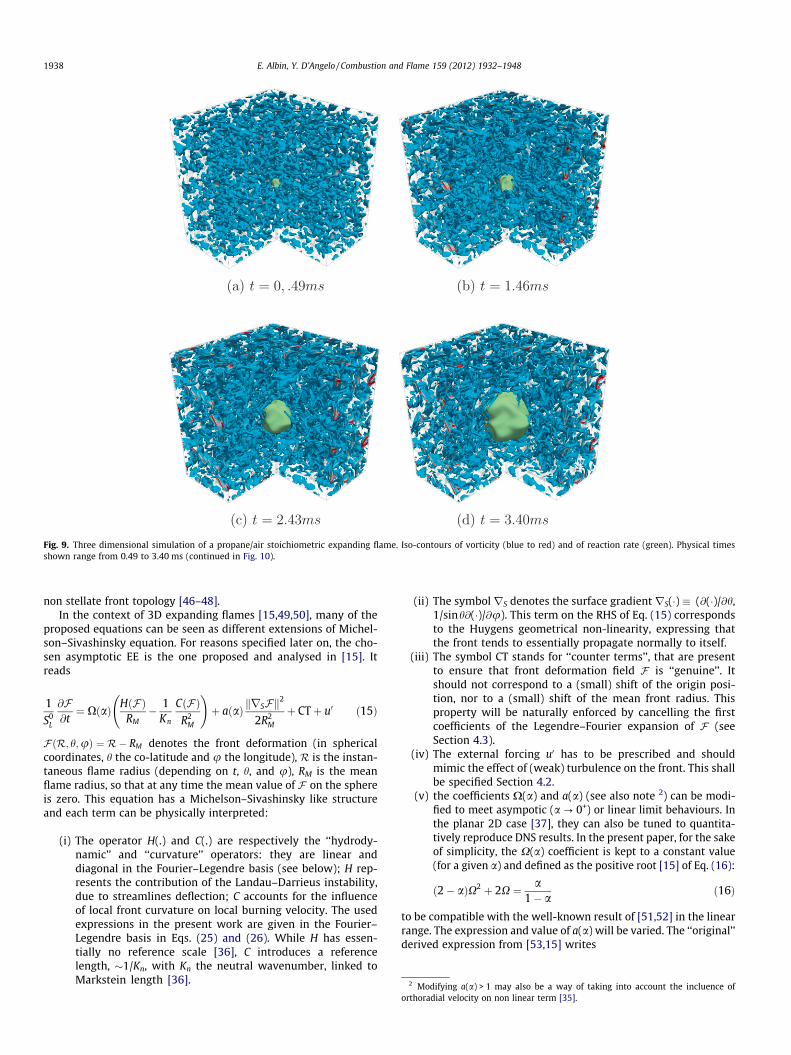
Fig. 9. Three dimensional simulation of a propane/air stoichiometric expanding flame. Iso-contours of vorticity (blue to red) and of reaction rate (green). Physical timesshown range from 0.49 to 3.40 ms (continued in Fig. 10).

2 Modifying a(a) > 1 may also be a way of taking into account the incluence of


non stellate front topology [46–48].In the context of 3D expanding flames [15,49,50], many of the

proposed equations can be seen as different extensions of Michel-son–Sivashinsky equation. For reasons specified later on, the cho-sen asymptotic EE is the one proposed and analysed in [15]. Itreads

1S0

L

@F@t¼ XðaÞ HðFÞ

RM� 1

Kn

CðFÞR2

M

!þ aðaÞ krSFk2

2R2M

þ CTþ u0 ð15Þ

FðR; h;uÞ ¼ R� RM denotes the front deformation (in sphericalcoordinates, h the co-latitude and u the longitude), R is the instan-taneous flame radius (depending on t, h, and u), RM is the meanflame radius, so that at any time the mean value of F on the sphereis zero. This equation has a Michelson–Sivashinsky like structureand each term can be physically interpreted:

(i) The operator H(.) and C(.) are respectively the ‘‘hydrody-namic’’ and ‘‘curvature’’ operators: they are linear anddiagonal in the Fourier–Legendre basis (see below); H rep-resents the contribution of the Landau–Darrieus instability,due to streamlines deflection; C accounts for the influenceof local front curvature on local burning velocity. The usedexpressions in the present work are given in the Fourier–Legendre basis in Eqs. (25) and (26). While H has essen-tially no reference scale [36], C introduces a referencelength, �1/Kn, with Kn the neutral wavenumber, linked toMarkstein length [36].

(ii) The symbolrS denotes the surface gradientrS(�) � (@(�)/@h,1/sinh@(�)/@u). This term on the RHS of Eq. (15) correspondsto the Huygens geometrical non-linearity, expressing thatthe front tends to essentially propagate normally to itself.

(iii) The symbol CT stands for ‘‘counter terms’’, that are presentto ensure that front deformation field F is ‘‘genuine’’. Itshould not correspond to a (small) shift of the origin posi-tion, nor to a (small) shift of the mean front radius. Thisproperty will be naturally enforced by cancelling the firstcoefficients of the Legendre–Fourier expansion of F (seeSection 4.3).

(iv) The external forcing u0 has to be prescribed and shouldmimic the effect of (weak) turbulence on the front. This shallbe specified Section 4.2.

(v) the coefficients X(a) and a(a) (see also note 2) can be modi-fied to meet asympotic (a ? 0+) or linear limit behaviours. Inthe planar 2D case [37], they can also be tuned to quantita-tively reproduce DNS results. In the present paper, for the sakeof simplicity, the X(a) coefficient is kept to a constant value(for a given a) and defined as the positive root [15] of Eq. (16):

orthora

ð2� aÞX2 þ 2X ¼ a1� a

ð16Þ

to be compatible with the well-known result of [51,52] in the linearrange. The expression and value of a(a) will be varied. The ‘‘original’’derived expression from [53,15] writes

dial velocity on non linear term [35].

Fig. 10. Three dimensional simulation of a propane/air stoichiometric expanding flame. Iso-contours of vorticity (blue to red) and of reaction rate (green). Physical timesrange here from 4.37 to 7.28 ms.

(a)

Z (

cm)

−1

−0.5

0

0.5

1

1.5

−1.5 −1 −0.5 0 0.5 1 1.5*

*

Y (cm)

−1.5

(b)

Z (

cm)

−1

−0.5

0

0.5

1

1.5

−1.5 −1 −0.5 0 0.5 1 1.5

X (cm)

*

*

−1.5

(c)

*

−1

−0.5

0

0.5

1

1.5

−1.5 −1 −0.5 0 0.5 1 1.5

X (cm)

Y (

cm)

*

−1.5

Fig. 11. DNS of an expanding flame: sections of iso-levels of temperature as a function of time. The three sections (a), (b) and (c) correspond respectively to YZ, XZ and XYplanar sections. Each contour is separated by a time step of 0.6 ms.


aðaÞ ¼ 22� a

ð17Þ

For a = 0.85, we obtain a ’ 1.74. Another expression, yielding the‘‘best fit’’ results for two-dimensional planar flames compared tonumerical simulations [36,37], is given by Eq. (18):

afitðaÞ ¼ 1þ 12aþ 3

8a2 þ 4

3ð1� aÞ�1=4 � 1þ a

4þ 5a2

32

� �� ð18Þ

For a = 0.85, we obtain afit ’ 2.07.

Eq. (15) appears as simple — it is a differential-like equation inthe Fourier–Legendre basis, even if the elliptic operator H(�) is nonlocal in space — and in a sense minimal in its structure — eachbuilding block has to be present to pertinently describe thephysics. As mentioned above, and shown in Section 4.3, it is first-order in time, a quite clear (and simple) physical meaning can be


associated to each present term,3 and it is computationally easy tohandle in the Fourier–Legendre spherical harmonics basis. Moreover,it is also robust against educated changes in the modelling [15]. Asmentioned in the introduction, it requires few (3 + turbulent forcing)and easy to change input parameters. Since it provides an equationfor the whole deformed sphere — including the poles — it has alsobeen refered to as ‘‘accurate’’ in Ref. [50].4

Note however that Eq. (15) needs to be supplemented with anevolution equation for the mean surface [15] (i.e. here for the meanfront radius RM). In [36,15], it is assumed that this mean radiusevolves as

dRM

dt¼ S0

L

1� að19Þ

i.e. wrinkling does not affect flame propagation velocity. In mostflamelet-based RANS or LES modelling [18], it is assumed that theeffective turbulent consumption rate is proportional to the flamesurface density or density of wrinkling (ibidem, Eq. (5.4)). In thequasi-planar case, it can be asymptotically derived, for a largeZel’dovitch number and a unity Lewis number [37]), that for steadyflame shapes the speed at which the front advances on average to-wards the fresh mixture is proportional to the flame surface in-crease. Using this argument, for large radii expanding flames5 (i.eRM�Markstein lengths), Eq. (19) can be combined with this qua-si-planar limit to yield

dRM

dt¼ S0

L

1� aAS ð20Þ

with AS ¼ SðtÞ4pR2

Mand S(t) the actual flame surface area. Here, we are

interested in initially small radii flames (RM ranging from 2 mm to2 cm, to be compared with Markstein lengths �100 lm), hence cur-vature and stretch effects are important, especially at early times.Combining equations (20) — for large wrinkled expanding flames— and (10) — for laminar stretched flames, and n = 2 in the sphericalcase — we propose

dRM

dt¼ S0

L

1� a� 11þ 2Lb=RM

� ASðtÞ ð21Þ

as evolution equation for the mean flame front RM. When AS ? 1(i.e. in absence of wrinkling), Eq. (21) yields (10), while whenRM�Markstein lengths (for larger radius flames), one gets Eq. (20).

The input parameters of the modelling are the following: thedensity contrast a, the laminar flame velocity S0

L and the Marksteinlength Lu. From these, one can deduce the neutral wavenumber Kn

[54]

Kn ¼a

2ð1� aÞLC’ a

2ð1� aÞLb¼ a

2Luð22Þ

One should also provide an external forcing term u0, mimicking tur-bulence, that will be specified next subsection.

4.2. External forcing

To mimic the effect of turbulence on the front, an additive forc-ing u0 (� the radial velocity component of the unburned mixture atthe front) can be introduced. Since for weak turbulence, the flameacts as a band-pass filter for wave numbers around K = Kn/r, with

3 Of course, combustion physics is richer than that! But, as this will be outlined inthe paper, the main features can be quantitatively captured by the modelling.

4 This reference proposed an interesting Fourier–Fourier modelling on largeequatorial sectors, but not including poles.

5 Notice that the ‘‘large’’ flames we are interested in the present paper are quite faraway from a fractal behaviour (RM � tm, with m ’ 1.5); cf. e.g. [13] as already refered toin the introduction.

6 The value of r, coming from the analysis on the linear range [15] is alsodepending on turbulence decaying time s; see Section 5.

r � 5 or 66 a simple uncorrelated white noise would do the job[15,54,55,43]. However, a more realistic turbulent forcing wouldbe both correlated in space and time [36]. In the present study, wemade the EEM evolve in the same (statistically speaking) Passot–Pouquet ‘‘turbulent’’ flow as the one used to initialize turbulencein the DNS, possibly with the same or different random seeds usedto generate it. To mimic turbulence temporal decay, we simply madethe velocity components exponentially decrease with time, as it willbe precised in Section 5. Notice that — at this stage — the modellingdoes not include flame retroaction on turbulence.

4.3. Numerical strategy

In the spectral Fourier–Legendre space, the evolution Eq. (15)can formally be cast as

@v lm

@t¼ Lv lm þ Nlm ð23Þ

where L is a linear operator and Nlm denotes the Fourier–Legendrecoefficient of the non linear term of (15), including the externalforcing; vlm denotes the l �m coefficient (in the spherical harmonicsbasis Ym

l ) of F (Eq. (15)) and

Lv lm �hðlÞRM� 1

Kn

cðlÞR2

M

ð24Þ

with

hðlÞ ¼ 2lðl� 1Þ2lþ 1

ð25Þ

and

cðlÞ ¼ ðl� 1Þðlþ 2Þ ð26Þ

as specified in Ref. [15]. As mentioned in Section 4.1 (item iii), thefirst terms are forced to zero (v00 = v10 = v11 = 0) to ensure ‘‘genuine’’deformations only.

A quite convenient way to numerically solve equations of thesame kind as (23) is to use Exponential Time Differencing Run-ge–Kutta (ETDRK) methods [56–59]. If h denotes the (assumedconstant) time step size, the first order and fourth order schemes[58] can respectively be written as

vnþ1 ¼ eLhvn þeLh � 1

LNn ð27Þ

and

an ¼ vneLh=2 þ eLh=2 � 1L

Nn; Na ¼ NðanÞ ð28aÞ

bn ¼ vneLh=2 þ eLh=2 � 1L

Na; Nb ¼ NðbnÞ ð28bÞ

cn ¼ aneLh=2 þ eLh=2 � 1L

ð2Nb � NnÞ; Nc ¼ NðcnÞ ð28cÞ

vnþ1 ¼ vneLh þ Nn

L3h2 ð�4� Lhþ eLhð4� 3Lhþ L2h2ÞÞ

þ 2ðNa þ NbÞL3h2 ð2þ Lhþ eLhð�2þ LhÞÞ

þ Nc

L3h2 ð�4� 3Lh� L2h2 þ eLhð4� LhÞÞ ð28dÞ

When computing terms of the form (ez � 1)/z with jzj? 0 numeri-cal cancellation errors may lead to unacceptable inaccuracy orinstability [58]. Following [58,57], in order to avoid these errorsfor small values of jLhj, the numerical evaluation of (ez � 1)/z makesuse of a contour integral in the complex plane around z = 0. Preli-


minary tests on one-dimensional Michelson–Sivashinsky equation[23] showed it was more convenient to use the ETDRK4 methodin terms of stability and CPU effort. Since we compare our EEMcomputation (less than two CPU hours on a 3 GHz Xeon processor)to much heavier DNS computations (�70,000 CPU hours), we didnot try — in this preliminary validation study — to use fast and/orparallel spherical harmonics tools [60,61].

In order to compare the EEM simulations with the DNS compu-tations, we projected the velocity radial component from the 4803

DNS grid (�100 � 106 points) to a coarser 1003 = 106 grid and wereable to compute the input forcing u0 to the EE. The EE is then solvedon a Fourier–Legendre grid of 1313 � 1312 (’1.7 � 106) colocationpoints, up to 3 cm of diameter.

5. Results and discussion

5.1. Input parameters

To reproduce an expanding stoichiometric propane/air flame atroom pressure and temperature, the numerical value of the densitycontrast was taken as a = 0.85. For our 3D EEM simulations, thenumerical value of the neutral wavenumber Kn is depending onthe numerical values of the density contrast a and of the firstMarkstein length (Eq. (22)).

To obtain a suitable numerical value for the Markstein lengthLu, we plot in Fig. 12 the mean consumption velocity SC (Eq. (3))vs. mean flame stretch k (Eq. (7)), for experimental results from[4] and also from present DNS calculation. Note that these resultswill also be reported in Fig. 13f), Fig. 14f), Fig. 15f) and Fig. 16f)for comparison with EEM results. To get a consistent comparison,we performed some equatorial sections of the DNS profiles, as itis actually done in the experiments, and extract SC and k fromthem. Table 2 gathers the obtained results, along with the deducedlaminar flame velocity (value of SC extrapolated at zero stretch).For our mixture, the unstretched laminar flame velocity isS0

L ¼ 0:407 m s�1. In this turbulent case, these values are quite dif-ficult to determine experimentally [18] and are subject to statisti-cal variation. As it can be observed, they indeed noticeably differfrom one section (including experiment) to another. Still, the ob-tained results are compatible with the values determined in thelaminar case (cf. Table 1, S0

L ’ 0:41 m s�1 and Lu � 120 lm), specif-ically for large radii (small values of k).

To take into account the temporal decay of turbulence intensity,we multiplied the computed forcing u0 by an exponential factore�t/s with s = 13 ms. This behaviour was determined from the

0

5

10

15

20

25

30

35

40

500 600 700 800 900 1000 1100 1200

S C (

cm/s

)

k (1/s)

DNS cut (a)DNS cut (b)DNS cut (c)

EXP.

Fig. 12. Evolution of mean consumption SC as a function of stretch k, for threeorthogonal sections of 3D turbulent expanding flame computation (denoted DNScut (a–c)).

non reactive isotropic turbulent flow simulation, used to initializethe flow before ignition. However, the presence of the flame mod-ifies the turbulent flow, and this is not taken into account by thepresent EEM approach. As this will be presented Section 5.3, a bet-ter agreement between DNS, EEM and EXP results was obtainedwhen decreasing the effective forcing felt by the flame by a factorb = 0.6 (see next subsection). Combined with the turbulence decayrate, the actual forcing u0a implemented in the simulation isu0a ¼ u0 � be�t=s. Moreover, in [36,37], in the context of 2D planarflames, the coefficient a(a) in the Michelson-Sivashinsky equation(equivalent to the a(a) in Eq. (15)) was tuned as a function of a inorder to fit the front winkling amplitude and successfully repro-duce DNS results.

5.2. Sensitivity to small changes on input parameters, robustness

To check the robustness and well-posedness of the modelling —do small changes in the input parameters induce small changes inthe outputs? — we ran different EEM simulations by slightlychanging the values of some input parameters around their nomi-nal or assumed value, which are not precisely known. Theseparameters were respectively a(a) — appearing in Eq. (15) — theMarsktein length Lu — linked to Kn via Eq. (22) — and u0/SL — theeffective intensity of the forcing felt by the flame, via the bparameter.

The ‘‘original’’ value [15] for a(a) (� 2/(2 � a) ’ 1.739 fora = 0.85) was modified to its fitted value in the planar case from[36,37] to give afit(a) ’ 2.071 for a = 0.85. We also tried an arbitrarylarger value a = 2.5. The numerical value for Lu was taken as 100,120 and 138 lm respectively, since the determined values for thisparameter (both from DNS and EXP) show a quite important dis-persion (as it is well known [18]) but still of the order of 100 lm.As already said in previous subsection, the b parameter was tunedfrom 1.0 to 0.6. This parameter may be seen as a correction for ret-roaction effect of the flame on turbulence, which is not taken intoaccount in the present approach. Indeed, a laminar expandingflame radius R essentially grows like dR=dt ¼ Sb ¼ quS0

L=qb (cf. Eq.(2) or (9)). Fixed vortices of size ‘ would then be consumed in atime � ‘/Sb, whereas a real flame would consume them in a time� ‘=S0

L since gas expansion pushes away the vortices in the radialdirection at a speed Sb � S0

L and also stretches them in the orthora-dial directions. For wrinkled flames not departing too much from aspherical shape, a practical way of taking into account gas expan-sion would be to elongate of a factor qu/qb in the radial directionthe non moving vortices seen by the flame [36]. The intensity de-crease of the synthetic forcing, via the b parameter, may constitutea simple way to take into account this ‘‘Doppler effect’’ on theflame propagation.

To ensure the robustness of the approach to statistical variation,we also changed the random seed parameters (used by the pseudo-random numbers generator) for the initial Passot–Pouquet spec-trum, corresponding to the four EEM samples in Figs. 13–16.

Finally, in the context of the present paper, we did not attemptany change of modelling for the curvature and hydrodynamicoperators expressions C and H [15], given in the Fourier–Legendrespace by Eqs. (25) and (26).

5.3. Comparison with DNS and experimental results

We quantitatively compared the resuts obtained with the EEMstrategy to the outputs from experiments [4] and present DNS re-sults (cf. Section 3).

Figure 13 shows the results obtained with the a priori chosen‘‘nominal’’ values of the parameters — that are in fact somewhatarbitrary — corresponding to Lu ¼ 138 lm; aðaÞ ¼ 2=ð2� aÞ’ 1:74 (Eq. (17)) and b = 1. Fig. 13a–f respectively show temporal

0

0.2

0.4

0.6

0.8

1

1.2

1.4

1.6

1.8

2

0 1 2 3 4 5 6 7

RP

(cm

)

time (ms)

EEM sample 1EEM sample 2EEM sample 3EEM sample 4


EXP.

(a)

0

0.2

0.4

0.6

0.8

1

1.2

1.4

1.6

1.8

0 1 2 3 4 5 6 7

RS

(cm

)

time (ms)



EXP.

(b)

500

600

700

800

900

1000

1100

1200

0 0.2 0.4 0.6 0.8 1 1.2 1.4

k (1

/s)

RS (cm)



EXP.

(c)

0

5

10

15

20

25

30

35

40

0 0.2 0.4 0.6 0.8 1 1.2 1.4

S C (

cm/s

)

RS (cm)



EXP.

(d)

0

5

10

15

20

25

30

35

40

45

0 0.2 0.4 0.6 0.8 1 1.2 1.4

S T (

cm/s

)

RS (cm)



EXP.

(e)

0

5

10

15

20

25

30

35

40

500 600 700 800 900 1000 1100 1200

S C (

cm/s

)

k (1/s)



EXP.

(f)Fig. 13. Comparison of DNS, EEM and experimental results from [4]. Time evolution of radii RP (a) and RS (b); evolution of stretch k (c), consumption speed SC (d) and meanturbulent velocity ST (e) as a function of RS; evolution of SC as a function of k (f). The set of used input parameters is: Lu ¼ 138 lm; aðaÞ ¼ 2=ð2� aÞ ’ 1:74 (from Ref. [15],b = 1.


evolution of radii RP and RS, mean stretch k, consumption speed SC

and mean turbulent velocity ST as functions of RS, and SC as a func-tion of k. The results from the experiments (quoted as EXP) arethose of [4]. The four equatorial sections from EEM are obtainedthanks to four different random seeds for the Passot–Pouquet spec-trum. Results obtained by DNS refer to three different orthogonal

sections of the 3D expanding simulation. While results betweenDNS and EXP are quite in line (except for difficult-to-determineoutputs like SC, ST and k), results from EEM, even if compatible,are slightly shifted to higher values, indicating the external forcingfelt by the flame may be too large. To correct this too large turbu-lent input, we decreased the b parameter from 1. to 0.6. Results,

0

0.2

0.4

0.6

0.8

1

1.2

1.4

1.6

1.8

0 1 2 3 4 5 6 7

RP

(cm

)

time (ms)



EXP.

(a)

0

0.2

0.4

0.6

0.8

1

1.2

1.4

1.6

0 1 2 3 4 5 6 7

RS

(cm

)

time (ms)



EXP.

(b)

500

600

700

800

900

1000

1100

1200

0 0.2 0.4 0.6 0.8 1 1.2 1.4

k (1

/s)

RS (cm)



EXP.

(c)

0

5

10

15

20

25

30

35

40

0 0.2 0.4 0.6 0.8 1 1.2 1.4

S C (

cm/s

)

RS (cm)



EXP.

(d)

0

5

10

15

20

25

30

35

40

45

0 0.2 0.4 0.6 0.8 1 1.2 1.4

S T (

cm/s

)

R S (cm)



EXP.

(e)

0

5

10

15

20

25

30

35

40

500 600 700 800 900 1000 1100 1200

S C (

cm/s

)

k (1/s)



EXP.

(f)Fig. 14. Comparison of DNS, EEM and experimental results from [4]. Time evolution of radii RP (a) and RS (b); evolution of stretch k (c), consumption speed SC (d) and meanturbulent velocity ST (e) as a function of RS; evolution of SC as a function of k (f). The set of used input parameters is: Lu ¼ 138 lm; aðaÞ ¼ 2=ð2� aÞ ’ 1:74 and b = 0.6.


similar to those of Fig. 13, are presented on Fig. 14. Quite fair agree-ment is now obtained between EEM, DNS and EXP results, in par-ticular at large radii and small stretch. Dispersion of resultsbetween the three sections of the one-shot DNS expensive compu-tation is compatible both with EXP and EEM results.

As mentioned Section 5.2, to test the sensitivity of the results tothe input parameters values we made some input parameters vary.We first varied the value of Marstein length Lu, which is known to

be difficult to determine [18], down to 120 and 100 lm. The re-sults, similar to the one of Fig. 14 are shown Fig. 15 forLu ¼ 100 lm. They indicate a quite low sensitivity of the resultsto this parameter. For the sake of brevity, figures forLu ¼ 120 lm, a ’ 1.74 and b ’ 0.6, which present quite close pro-files to those of Fig. 14 are not shown. This may be seen as a com-forting argument to the EEM approach: the Lu input parameter isdifficult to evaluate but does not influence much the quantitative

0

0.2

0.4

0.6

0.8

1

1.2

1.4

1.6

1.8

2

0 1 2 3 4 5 6 7

RP

(cm

)

time (ms)



EXP.

(a)

0

0.2

0.4

0.6

0.8

1

1.2

1.4

1.6

0 1 2 3 4 5 6 7

RS

(cm

)

time (ms)



EXP.

(b)

500

600

700

800

900

1000

1100

1200

0 0.2 0.4 0.6 0.8 1 1.2 1.4

k (1

/s)

RS (cm)



EXP.

(c)

0

5

10

15

20

25

30

35

40

0 0.2 0.4 0.6 0.8 1 1.2 1.4

S C (

cm/s

)

RS (cm)



EXP.

(d)

0

5

10

15

20

25

30

35

40

45

0 0.2 0.4 0.6 0.8 1 1.2 1.4

S T (

cm/s

)

RS (cm)



EXP.

(e)

0

5

10

15

20

25

30

35

40

500 600 700 800 900 1000 1100 1200

S C (

cm/s

)

k (1/s)



EXP.

(f)Fig. 15. Comparison of DNS, EEM and experimental results from [4]. Time evolution of radii RP (a) and RS (b); evolution of stretch k (c), consumption speed SC (d) and meanturbulent velocity ST (e) as a function of RS; evolution of SC as a function of k (f). The set of used input parameters is: Lu ¼ 100 lm; aðaÞ ¼ 2=ð2� aÞ ’ 1:74, b = 0.6.


observed results. More specifically, the Lu input parameter inter-venes, via Kn (see Eq. (22)), in the scaling of radius RM, front defor-mation F and time t [15]. Since the actual (experimental) value ofthe initial kernel is not known, the chosen initial value for the frontradius is given by a constant scaled value of 5, corresponding to adimensional value of approximately 1.2–1.6 mm, depending on Lu.

As emphasized in Section 2, front contour is very difficult to deter-mine for these small values of radii. At early times (�0.2 ms), theEEM computed uncorregated front radii RS and RP are indeed inthe correct ratios of 138/100 or 120/100, as expected.

As already mentioned, the coefficient a(a) was also increased toits ‘‘planar best-fit’’ value of 2.07 [37] for a = 0.85, corresponding to

0

0.2

0.4

0.6

0.8

1

1.2

1.4

1.6

1.8

0 1 2 3 4 5 6 7

RP

(cm

)

time (ms)



EXP.

(a)

0

0.2

0.4

0.6

0.8

1

1.2

1.4

1.6

0 1 2 3 4 5 6 7

RS

(cm

)

time (ms)



EXP.

(b)

500

600

700

800

900

1000

1100

1200

0 0.2 0.4 0.6 0.8 1 1.2 1.4

k (1

/s)

RS (cm)



EXP.

(c)

0

5

10

15

20

25

30

35

40

0 0.2 0.4 0.6 0.8 1 1.2 1.4

S C (

cm/s

)

RS (cm)



EXP.

(d)

0

5

10

15

20

25

30

35

40

45

0 0.2 0.4 0.6 0.8 1 1.2 1.4

S T (

cm/s

)

RS (cm)


DNS cut (b)DNS cut (c)

EXP.

(e)

0

5

10

15

20

25

30

35

40

500 600 700 800 900 1000 1100 1200

S C (

cm/s

)

k (1/s)



EXP.

(f)Fig. 16. Comparison of DNS, EEM and experimental results from [4]. Time evolution of radii RP (a) and RS (b); evolution of stretch k (c), consumption speed SC (d) and meanturbulent velocity ST (e) as a function of RS; evolution of SC as a function of k (f). The set of used input parameters is: Lu ¼ 120 lm; aðaÞ ’ 2:07 (best fit for planar flames, cf.[37]) and b = 0.6.


Eq. (18). For this case, we plot on Fig. 16 the results obtained bysimultaneously varying the Lu parameter down to 120 lm. Again,the results are quite similar to the one of Fig. 14. We also tried toincrease the value of a even more, up to the arbitrary value of 2.5,without noticing any qualitative change in the results. For the sakeof brevity, these results are not shown here.

Finally, we compare EEM with DNS results of Figs. 9 and 10 andcorresponding equatorial sections of Fig. 11. Figure 17 show thetime evolution of 3D contours of a sample EEM computation whileFig. 18 show the temporal evolution of equatorial sections.Although the EEM front may seem slightly more corrugated, the vi-sual resemblance is striking.

Table 2Determination of laminar flame velocity S0

L (extrapolated value at zero stretch) and ofthe first Markstein length Lu from data of Fig. 12.

Case S0L ðcm=sÞ Lu ðlmÞ

DNS cut (a) 44.7 154DNS cut (b) 41.4 123DNS cut (c) 39.3 107Experiment [4] 35.9 107

Fig. 17. Sample numerical simulation of an expanding flame by the EEM approach. To ecorresponding times are respectively 2.01, 3.33, 4.65, 5.44, 6.49 and 7.28 ms. The corresinput parameters is: Lu ¼ 138 lm; aðaÞ ¼ 2=ð2� aÞ ’ 1:74 and b = 0.6. This figures are


It is known that expanding wrinkled flames present strongangular invariance, both in experiments [8] and DNS computa-tions, despite the external (but quite moderate) turbulent forcing.This means that no intrinsic reference length actually plays animportant role in the expansion. The only length scale present inthe system (apart from the external turbulence integral scale) isthe laminar flame thickness or equivalently the Markstein length.As already mentioned, the role of this lengthscale is actually to

ase readability, the mean radius has been rescaled to max size for each figure. Theponding mean radii are (in mm) 3.58, 6.26, 9.23, 11.1, 13.7 et 15.5. The set of usedto be compared with the results from Figs. 9 and 10.

0.015

0.01

0.005

0

0.005

0.01

0.015

0.015 0.01 0.005 0 0.005 0.01 0.015 0.015

0.01

0.005

0

0.005

0.01

0.015

0.015 0.01 0.005 0 0.005 0.01 0.015

Fig. 18. EEM strategy: two equatorial sections of the expanding front for two different realizations of Passot–Pouquet forcing (corresponding to samples 1 and 2 of Fig. 14) forLu ¼ 138 lm; b ¼ 0:6 and a = 1.74. The time interval between two isolines is Dt = 0.376ms). These figures are to be compared with DNS results of Fig. 11.

7 The corresponding local velocities induced by front deformation can be deter-mined [37].


smooth the crests present on the front surface. In that sense, noreference length plays an important role in the expansion (formoderate turbulent forcing) and the observed angular invarianceis a signature of the Landau–Darrieus instability, that has no refer-ence length. The exact value of the Markstein length is hence ‘‘for-gotten’’ by the system [36]. This feature is well captured by thepresent EEM approach. Of course, this will not hold true for highlevels of turbulent forcing: another reference length — e.g. the tur-bulence integral scale — will then appear, or when other instabili-ties (like the thermo-diffusive instability) are present.

Also notice that in the present EEM approach, one does not solvefor the turbulent flow, nor flame front retroaction on the flow. Theflame front structure is not resolved either. That is why the approachis so unexpensive. Moreover, the ‘‘turbulent noise’’ we are providingto the EEM is a Passot–Pouquet synthetic forcing. Hence, the ‘‘real’’turbulence ‘‘felt’’ by the flame is not known exactly. We think —and the obtained results of the present paper tend to support this— that we can actually lump all these effects by only modifyingthe effective amplitude of the forcing felt by the flame in the EEM ap-proach. Even if clearly connected to the adopted synthetic noise,adjusting only the two parameters s and b seemed to be sufficientto reproduce quantitative results. To compute large scale expandingflames (for a given mixture) an overall efficient procedure may con-sist in: (i) compute small scale flames with a DNS solver, to deter-mine and adjust the corresponding s and b parameters; (ii)proceed with the EEM strategy — that seems to include all the nec-essary ingredients for this — to compute efficiently much largerflames, presently out of reach for nowadays DNS.

6. Concluding remarks

The present paper quantitatively compared in-house DNS re-sults, EEM computations and experimental results from literaturefor a propane-air three-dimensional expanding flame. The experi-mental results were taken from references [4,8]. Making use ofthe same post-processing smoothing procedure, we were able tocompare experimentally determined equivalent radii RP and RS,mean stretch k, consumption velocity SC and mean displacementspeed ST. Sample front shapes and equatorial sections from DNSand EEM were also compared. Although they may be quite difficultto measure in practice, we focused on these output quantities be-cause they are of interest for experiments and practical applica-

tions. For large enough flames, post-processing of DNS and EEMdata should also allow comparing and analysing other outputs, likee.g. cell size distribution on the front [62,63].

As it can be observed, obtained quantitative agreement is verygood, especially between DNS and EEM. However, the present cal-culation and experiments do not deviate much from a quasi-lineartemporal expansion for the front. The regime where the flameaccelerates (R � t 3/2 [13]) is very difficult to handle by means ofDNS, since it requires to attain large radii and hence demands ahuge computational effort. However, since we demonstrated thatthe present EEM strategy quantitatively compares both with DNSand EXP results, EEM can now be applied to simulations of largerspherical flames. The well-captured coupling between cell forma-tion by weak turbulent forcing and Landau–Darrieus instability,and expansion — that tends to drive away cells one from anotherin the front surface — essentially contains the seed that may leadto front fractalization [36,15]. However, reaching such large sizesmay require, as suggested in [50], an efficient parallelization ofthe numerical algorithm, presently based on spherical harmonics[60,61].

Moreover, the modelling and analysis of other kinds of flameinstabilities, like the thermo-diffusive instability — see e.g. the re-cent numerical investigation for low Lewis number lean hydrogenflames [64,12] — should require a more elaborated Evolution Equa-tion Modelling, possibly including a fourth-order term, like in theKuramoto–Sivashinsky equation [65].

The EEM approach presented here is quite simple, but, as al-ready mentioned, is only limited to single valued fronts, i.e. onlymoderately wrinkled flames can be handled. Highly corrugatedmulti-valued fronts, or flames with pockets, cannot be describedwith this ‘‘simple’’ approach. As mentioned earlier, other (less sim-ple) strategies [46–48,41] can be thought of, and may deserve to beassessed too, but this was not the aim of the present paper. How-ever, these limitations may be circumvented and a possible exten-sion of the approach may consist in designing an EEM-basedsubgrid scale modelling for coarse-grid Large Eddy Simulations ofturbulent reactive flows [37]. Turbulent forcing and local flametopology may then be coupled i.e. local flame shape does interactwith local turbulence7 — this is not the case in the present model-


ling — via the local resolution of an Evolution Equation for the front.8

A pre-requisite would be the assessment of 3D planar flames evolu-tion equations [43,44], possibly including thermo-diffusive effects.

Acknowledgements

The authors thank the reviewers for their valuable commentsand suggestions, and also Prof. B. Renou and Dr. B. Lecordier forfruitful discussions. The CPU time for DNS computations was freelyallocated by French CNRS Supercomputing Center (IDRIS) andHaute-Normandie Computing Center (CRIHAN).

References

[1] X. Gu, M. Haq, M. Lawes, R. Woolley, Combustion and Flame 121 (1–2) (2000)41–58.

[2] D. Bradley, R. Hicks, M. Lawes, C. Sheppard, R. Woolley, Combustion and Flame115 (1) (1998) 126–144.

[3] N. Peters, Symposium (International) on Combustion 21 (1) (1988) 1231–1250,doi:10.1016/S0082-0784(88)80355-2.

[4] B. Renou, Contribution à l’étude de la propagation d’une flamme deprémélange instationnaire dans un écoulement turbulent. Influence dunombre de Lewis., PhD thesis, INSA Rouen, 1999.

[5] O. Pajot, Etude expérimentale de l’influence de l’aérodynamique sur lecomportement et la structure du front de flamme dans les conditions d’unmoteur à allumage commandé., PhD thesis.

[6] F. Foucher, Etude expérimentale de l’interaction flamme-paroi: Application aumoteur à allumage commandé., PhD thesis.

[7] F. Foucher, S. Burnel, C. Mounaı̈m-Rousselle, Proceedings of the CombustionInstitute 29 (1) (2002) 751–757.

[8] B. Lecordier, Etude de l’interaction de la propagation d’une flammeprémélangée avec le champ aérodynamique par association de latomographie laser et de la vélocimétrie par images de particules., PhD thesis,Université de Rouen, 1997.

[9] G. Groot, L. De Goey, Proceedings of the Combustion Institute 29 (2) (2002)1445–1451.

[10] G. Groot, Modelling of Propagating Spherical and Cylindrical Premixed Flames,PhD Thesis.

[11] J. Oijen, R. Bastiaans, G. Groot, L. De Goey, Flow, Turbulence and Combustion75 (1) (2005) 67–84.

[12] C. Altantzis, Numerical Investigation of the Dynamics of Unstable LeanPremixed Hydrogen/Air Flames, PhD Thesis, ETHZ Zurich, 2011.

[13] Y. Gostintsev, A. Istratov, Y. Shulenin, Combustion, Explosion, and ShockWaves 24 (5) (1988) 63–70.

[14] L. Filyand, G. Sivashinsky, M. Frankel, Physica D: Nonlinear Phenomena 72 (1–2) (1994) 110–118, doi:10.1016/0167-2789(94)90170-8.

[15] Y. D’Angelo, G. Joulin, G. Boury, Combustion Theory and Modelling 4 (3) (2000)317–338.

[16] B. Renou, A. Boukhalfa, D. Puechberty, M. Trinité, Combustion and Flame 123(4) (2000) 507–521.

[17] B. Renou, A. Boukhalfa, Combustion Science and Technology 16 (2001) 347–370.

[18] T. Poinsot, D. Veynante, Theoretical and Numerical Combustion, R.T. EdwardsInc., 2005.

[19] F. Baillot, D. Durox, D. Demare, Proceedings of the Combustion Institute 29 (2)(2002) 1453–1460.

[20] F. Williams, A review of some theoretical considerations of turbulent flamestructure, AGARD Anal. and Numerical Methods for Invest. of Flow Fields withChem. Reactions, Especially Related to Combust. 25 p(SEE N 75-30359 21-31).

[21] T. Tahtouh, F. Halter, C. Mounaı̈m-Rousselle, Combustion and Flame 156 (9)(2009) 1735–1743.

[22] L. Vervisch, B. Labegorre, J. Réveillon, Fuel 83 (4–5) (2004) 605–614.[23] E. Albin, Contribution à la modélisation numérique des flammes turbulentes:

comparaisons dns-eem-expériences., Ph D Thesis.[24] E. Albin, Y. D’Angelo, L. Vervisch, Using staggered grids with characteristic

boundary conditions when solving compressible reactive Navier–Stokes

8 Notice that the Landau-Darrieus operator is non-local in space (the correspondingterm in the EEM has an elliptic contribution), but has in fact a localized range ofinfluence [36].

equations, International Journal for Numerical Methods in Fluids.doi:10.1002/fld.2520.

[25] C.S. Yoo, H.G. Im, Combustion Theory and Modelling 11 (2) (2007) 259–286.[26] T. Poinsot, S. Lele, Journal of Computational Physics 101 (1) (1992) 104–129.[27] G. Lodato, P. Domingo, L. Vervisch, Journal of Computational Physics 227 (10)

(2008) 5105–5143.[28] S. Davis, J. Quinard, G. Searby, Combustion and Flame 130 (1–2) (2002) 123–

136.[29] S. Marley, W. Roberts, Combustion and Flame 141 (2005) 473–477.[30] A. Lipatnikov, J. Chomiak, Progress in Energy and Combustion Science 31 (1)

(2005) 1–73.[31] D. Durox, S. Ducruix, S. Candel, Combustion and Flame 125 (1–2) (2001) 982–

1000.[32] T. Passot, A. Pouquet, Journal of Fluid Mechanics 181 (1987) 441–466,

doi:10.1017/S0022112087002167.[33] E. Albin, Y. D’Angelo, Effects of Navier–Stokes Characteristic Outflow Boundary

Conditions: Modeling for Transverse Flows, Proceedings of ECM 2011, Cardiff.[34] G. Sivashinsky, Acta Astronautica 4 (1977) 1177–1206.[35] G.I. Sivashinsky, P. Clavin, Journal de Physique France 48 (2) (1987) 193–198,

doi:10.1051/jphys:01987004802019300.[36] G. Boury, Etudes théoriques et numériques de fronts de flammes plissées:

dynamiques non-linéaires libres ou bruitées., PhD thesis, Université dePoitiers, 2003.

[37] G. Boury, Y. D’Angelo, On third order density contrast expansion of theevolution equation for wrinkled unsteady premixed flames, InternationalJournal of Non-Linear Mechanics. doi:10.1016/j.ijnonlinmec.2011.05.018.

[38] J. Dold, G. Joulin, Combustion and Flame 100 (1995) 450–456.[39] R. Rego, On a Non-linear Model of Flame/Acoustics Interaction, PhD Thesis,

University of Politiers, 2006.[40] K.A. Kazakov, Physics of Fluids 17 (3) (2005) 032107, doi:10.1063/1.1864132.[41] H. El-Rabii, G. Joulin, K.A. Kazakov, Physical Review Letters 100 (17) (2008)

174501, doi:10.1103/PhysRevLett.100.174501.[42] V.V. Bychkov, Physics of Fluids 10 (8) (1998) 2091–2098, doi:10.1063/

1.869723.[43] B. Denet, Physical Review E 75 (4) (2007) 46310.[44] V. Karlin, V. Maz’ya, G. Schmidt, Journal of Computational Physics 188 (1)

(2003) 209–231.[45] F. Creta, N. Fogla, M. Matalon, Combustion Theory and Modelling 15 (2) (2011)

267–298.[46] M. Frankel, Physics of Fluids A 2 (10) (1990).[47] B. Denet, Physical Review E 55 (6) (1997) 6911–6916, doi:10.1103/

PhysRevE.55.6911.[48] B. Denet, Physics of Fluids 16 (4) (2004) 1149–1155.[49] V. Karlin, G. Sivashinsky, Combustion Theory and Modelling 10 (4) (2006)

625–637.[50] V. Karlin, G. Sivashinsky, Proceedings of the Combustion Institute 31 (1) (2007)

1023–1030.[51] L. Landau, Acta Physicochimica URSS 19 (1944) 77–85.[52] G. Darrieus, Propagation d’un front de flamme, Unpublished work presented at

La Technique Moderne, and at Le Congrès de Mécanique Appliquée (1945).[53] G. Joulin, P. Cambray, Combustion Science and Technology 81 (1992) 243–256.[54] P. Cambray, K. Joulain, G. Joulin, Dynamique, propre ou bruitee, de flammes

plissees en expansion, Unpublished DRET report 93 (1996) 060.[55] G. Joulin, G. Boury, P. Cambray, Y. D’Angelo, K. Joulain, Lecture Notes in Physics

(2001) 127–158.[56] S. Cox, P. Matthews, Journal of Computational Physics 176 (2) (2002) 430–455.[57] Q. Du, W. Zhu, BIT Numerical Mathematics 45 (2) (2005) 307–328.[58] A. Kassam, L. Trefethen, SIAM Journal on Scientific Computing 26 (4) (2005)

1214–1233.[59] P. Livermore, Journal of Computational Physics 220 (2) (2007) 824–838.[60] R. Stompor, S2hat Parallel Scalable Spherical Harmonic Transform Package.[61] C. Cantalupo, ccsht: A Fast Parallel Spherical Harmonic Transform. <http://

crd.lbl.gov/cmc/ccSHTlib/doc/index.html>.[62] G. Jomaas, Propagation and Stability of Expanding Spherical Flames, PhD

Thesis, Princeton University, 2008.[63] J.K. Bechtold, M. Matalon, Combustion and Flame 67 (1987) 77–90.[64] C. Altantzis, C. Frouzakis, A. Tomboulides, S. Kerkemeier, K. Boulouchos,

Proceedings of the Combustion Institute 33 (1) (2011) 1261–1268,doi:10.1016/j.proci.2010.06.082.

[65] Y. Kuramoto, T. Tsuzuki, Progress of Theoretical Physics 55 (2) (1976) 356–369, doi:10.1143/PTP.55.356.

http://dx.doi.org/10.1016/S0082-0784(88)80355-2

http://dx.doi.org/10.1016/0167-2789(94)90170-8

http://dx.doi.org/10.1002/fld.2520

http://dx.doi.org/10.1017/S0022112087002167

http://dx.doi.org/10.1051/jphys:01987004802019300

http://dx.doi.org/10.1016/j.ijnonlinmec.2011.05.018

http://dx.doi.org/10.1063/1.1864132

http://dx.doi.org/10.1103/PhysRevLett.100.174501

http://dx.doi.org/10.1063/1.869723

http://dx.doi.org/10.1063/1.869723

http://dx.doi.org/10.1103/PhysRevE.55.6911

http://dx.doi.org/10.1103/PhysRevE.55.6911

http://crd.lbl.gov/cmc/ccSHTlib/doc/index.html

http://crd.lbl.gov/cmc/ccSHTlib/doc/index.html

http://dx.doi.org/10.1016/j.proci.2010.06.082

http://dx.doi.org/10.1143/PTP.55.356

assessment of the evolution equation modelling approach for three-dimensional expanding wrinkled...

Documents