Natural Resources Research ( C© 2007)DOI: 10.1007/s11053-007-9028-7

Assessment of the Enhanced Geothermal SystemResource Base of the United States

David D. Blackwell,1,2 Petru T. Negraru,1 and Maria C. Richards1

Received 18 June 2006; accepted 21 November 2006

This paper describes an assessment of the enhanced geothermal system (EGS) resource baseof the conterminous United States, using constructed temperature at depth maps. The tem-perature at depth maps were computed from 3 to 10 km, for every km. The methodology isdescribed. Factors included are sediment thickness, thermal conductivity variations, distribu-tion of the radioactive heat generation and surface temperature based on several geologicmodels of the upper 10 km of the crust. EGS systems are extended in this paper to includecoproduced geothermal energy, and geopressured resources.

A table is provided that summarizes the resource base estimates for all components ofthe EGS geothermal resource. By far, the conduction-dominated components of EGS rep-resent the largest component of the U.S. resource. Nonetheless, the coproduced resourcesand geopressured resources are large and significant targets for short and intermediate termdevelopment. There is a huge resource base between the depths of 3 and 8 km, where the tem-perature reaches 150–250◦C. Even if only 2% of the conventional EGS resource is developed,the energy recovered would be equivalent to roughly 2,500 times the annual consumption ofprimary energy in the U.S. in 2006. Temperatures above 150◦C at those depths are more com-mon in the active tectonic regions of the western conterminous U.S., but are not confined tothose areas. In the central and eastern U.S. there are identified areas of moderate size thatare of reasonable grade and probably small areas of much higher grade than predicted by thisanalyses. However because of the regional (the grid size is 5′ × 5′) scale of this study suchpotentially promising sites remain to be identified.

Several possible scenarios for EGS development are discussed. The most promising andleast costly may to be developments in abandoned or shut-in oil and gas fields, where thetemperatures are high enough. Because thousands of wells are already drilled in those loca-tions, the cost of producing energy from such fields could be significantly lowered. In additionmany hydrocarbon fields are producing large amounts of co-produced water, which is neces-sary for geothermal development. Although sustainability is not addressed in this study, theresource is so large that in at least some scenarios of development the geothermal resource issustainable for long periods of time.

KEY WORDS: Geothermal, geothermal resource base, renewable energy, heat generation, U.S. heatflow, temperature-at-depth, coproduced fluids, enhanced geothermal systems (EGS).

INTRODUCTION

Geothermal energy from areas with abundanthot water or steam has been developed extensively

1Geothermal Lab, Department of Geological Sciences, SouthernMethodist University, Dallas, TX 75275, USA.

2To whom correspondence should be addressed; e-mail: blackwel@smu.edu.

worldwide (Barbier, 2002). There is currently aninstalled capacity of more than 8,000 MW of hy-drothermal geothermal energy with an average loadfactor exceeding 95%. Hydrothermal geothermalenergy generally is considered to be developable iftemperatures exceed 150◦C and there is abundantproducible water (or steam). It generally is assumedthat such resources are exclusively related to areas

1520-7439/07 C© 2007 International Association for Mathematical Geology

Blackwell, Negraru, and Richards

of young volcanic activity and or high heat flowassociated with active tectonism and most of thedevelopments so far conform to this hypothesis.However, temperature increases with depth every-where and so in theory geothermal energy could bedeveloped almost anywhere. Of course, there arepractical limits to the possible depth of exploitation.There are several classes of geothermal resourcesthat might be considered possibilities for develop-ment in addition to the conventional hydrothermalones, particularly in view of the relatively benign en-vironmental effects, moderate cost of development,and ubiquity of possible locations compared to otherrenewable and nonrenewable systems capable ofgenerating electrical power (DiPippo, 1991a, 1991b;Mock, Tester, and Wright, 1997). The concept ofmaking an artificial reservoir and forming an artificialgeothermal system, initially termed Hot Dry Rockgeothermal energy has been investigated in manyareas with ongoing activity in Europe and Australia(Tester and others, 2006). A more general term isEnhanced Geothermal System (EGS) implying amore general scenario of development.

Previous analyses have suggested that theamount of thermal energy available for EGS devel-opment is enormous (Armstead and Tester, 1987;Rowley, 1982; Mock, Tester, and Wright, 1997;Tester and others, 1994). However, these sources didnot use detailed geologic information and, as a re-sult, the methodologies employed were by necessitysomewhat simplified. The primary focus of this pa-per is a detailed regional analysis of the heat contentin the upper crust in the conterminous U.S. as a re-source base evaluation of the potential for EGS en-ergy development. Although the results generally arelimited to the conterminous part of the U.S., Alaska,and Hawaii will be discussed briefly, in particularwith respect to the potential of the volcanic systems.

This analysis is the resource basis of a detailedand complete study recently published (Tester andothers, 2006) that considered in detail all aspects ofEGS development from resource base to cost to en-vironmental effects.

The various classes of geothermal developmentare listed in Table 1. Several categories of geother-mal resources listed in Table 1 were evaluated inthe 1970’s by the U.S. Geological Survey (Whiteand Williams, 1975; Muffler, 1979). In earlier USGSanalyses the geothermal resource was divided intofour major categories: hydrothermal, geopressured,magma, and conduction-dominated (Hot Dry Rock,HDR—now typically referred to as EGS). Table 1

Table 1. Geothermal Resource Categories. Modified from USGSCirculars 726 and 790

Resource Type Reference

Conduction-dominated (EGS)Sedimentary EGS (SEGS) This study, basins >4 kmBasement EGS This studyVolcano Geothermal Systems USGS Circular 790Hydrothermal USGS Circulars 726 and 790Co-produced Fluids McKenna and others (2005)Geopressured Systems USGS Circulars 726 and 790

also includes additional resource categories not men-tioned in the earlier assessments. In this paper wespecifically exclude detailed discussion of conven-tional hydrothermal resources, magma and geopres-sure geothermal resources. A resource evaluation forhydrothermal geothermal systems is in process by ateam at the U.S. Geological Survey (Williams, 2005).The classes of resource that are discussed in detail inthis paper are sedimentary and basement EGS.

Not included here because of their relativelysmall geographic size are “high grade” EGS Re-sources on the periphery of the conventional hy-drothermal systems in the western U.S. Most of thesetypes of targets are high grade and can be viewed asnear-term targets of opportunity. These areas may beconsidered more properly part of the ongoing USGShydrothermal resource assessment because of theirassociation and small size. However, some largerbasement EGS resource areas that might in somesense be considered marginal to hydrothermal sys-tems, such as The Geysers/Clear Lake area in Cali-fornia and the High Cascades Range in Oregon, areincluded in this assessment because of their largesize.

The primary object of this study is to calculatethe stored thermal energy, or “heat” in place nation-ally and by state at depths from 3 to 10 km. Themethodology, resource types considered, and the re-source base calculations are included in this paperand follow Chapter 2 of Tester and others (2006).Recoverability, or useful energy, is not addressed indetail in this paper.

SOURCE OF DATA

The data set used to produce the GeothermalMap of North America published by the Ameri-can Association of Petroleum Geologists (AAPG)(Blackwell and Richards, 2004a) is the basic thermal

Assessment of the Enhanced Geothermal System Resource Base of the United States

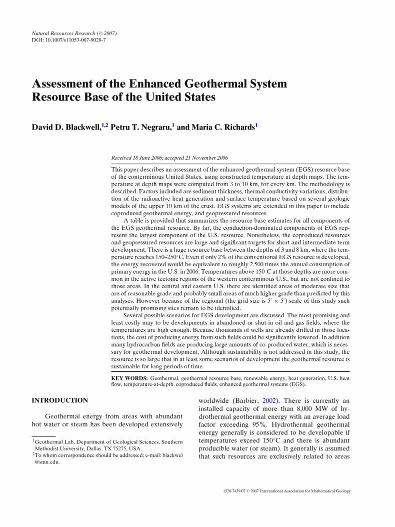
Figure 1. Heat Flow map of conterminous United States. Subset of Geothermal map of North America (Blackwell and Richards,2004a).

data set used in developing this resource assess-ment. The conterminous U.S. portion of the map isshown in Figure 1. In order to expand coverage fromthe GSA-DNAG map (Blackwell and Steele, 1992;Blackwell, Steele, and Carter, 1991) and previousmethods of resource evaluation (Blackwell, Steele,and Carter, 1993; Blackwell, Steele, and Wisian,1994), extensive industry-oriented thermal data setswere used, as well as published heat-flow data fromresearch groups. To that end a Western U.S. heatflow data set was developed, based on thermal gra-dient exploration data collected by the geothermalindustry during the 1970’s and 1980’s (Blackwell andRichards, 2004c) and the 1974 AAPG Bottom HoleTemperature (BHT) data set (AAPG CD-ROM,1994) was processed for temperature at depth andheat-flow determinations.

The basic information in the Western U.S. heat-flow data set consists of temperature-depth/gradientinformation. However, thermal conductivity andheat flow also were determined for as many of thesites as possible, based on thermal conductivity mea-surements, or estimates from geologic logs (whereavailable) and geologic maps for locations with nowell logs. About 4,000 points were used in the prepa-

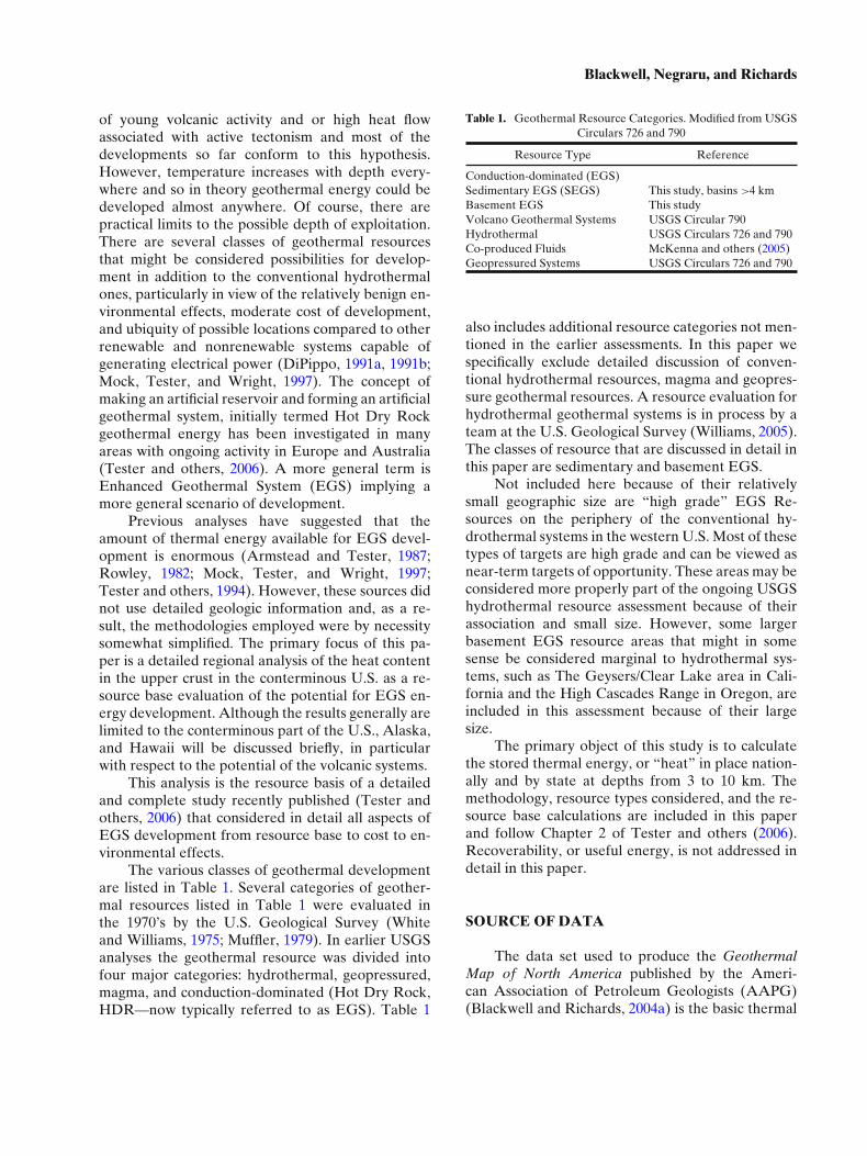
ration of the map (of the 6,000 sites in the database).The focused nature of the drilling is shown by theclumps of data on Figure 2, especially in westernNevada and southwestern Utah.

A second industry data set consisting of about12,000 bottom hole temperature measurements com-piled in the early 1970’s and published in digital form(DeFord and Kehle, 1976; AAPG CD-ROM, 1994)also was utilized. The AAPG BHT data set was aug-mented in Nevada by BHT data digitized from hy-drocarbon exploration well logs in the files of theNevada Bureau of Mines and Geology. Use of theBHT data required extensive analysis of the errorassociated with the determination of in situ equilib-rium temperatures from these nonequilibrium data(Blackwell and Richards, 2004b, 2004c).

The heat flow ranges from less than 20 mW/m2

in areas of low heat flow to above 100 mW/m2 in ar-eas of high heat flow. The causes of the variationsand the distribution of heat flow in the conterminousU.S. are discussed by Blackwell, Steele, and Carter(1991) and Morgan and Gosnold (1989). The value ofsurface heat flow is the building block for the tem-perature at depth calculation. Figure 2 also illustratesthat at the present stage of the analysis there are

Blackwell, Negraru, and Richards

Figure 2. All BHT sites in the conterminous U.S. in the AAPG data base. BHT symbols are based on depth and temperature (not all ofthe sites were used for the Geothermal Map of North America). The named wells are the calibration points. The regional heat flow andgeothermal database sites are also shown.

large geographic areas that are under-sampled withrespect to the 5′ grid interval, such that aliasing lo-cally is a problem that leads to uncertainty. For ex-ample, Kentucky and Wisconsin have no heat flowdata at all and there are large gaps in several otherareas, especially the eastern part of the U.S. Ar-eas in the Appalachian basin may have low thermalconductivity and high heat flow, as is the situationin northwestern Pennsylvania, but there are limiteddata in this region. A typical 250 MWe (electrical)EGS plant might require about 5–10 km2 of reservoirplanar area to accommodate the thermal resourceneeded, assuming that heat removal occurs in a 1 kmthick region of hot rock at depth. The power plantoperations, of course, would be confined to a muchsmaller area, 3 km2 or less (Tester and others, 2006,chapter 3). Thus, at the field level, specific explo-ration and evaluation activity will be necessary to se-lect optimum sites in a given region.

To summarize, the values of heat flow used toproduce the contours for the U.S. (shown in Fig. 1)were compiled from the following data sets: the SMUWestern Geothermal database (includes the USGS

Great Basin database, http://wrgis.wr.usgs.gov/open-file/of99-425/webmaps/home.html), the SMU com-piled U.S. Regional Heat Flow database (www.smu.edu/geothermal), and American Assocation Petro-leum Geologists BHT (AAPG CD-ROM, 1994). Thevarious data site locations are shown in Figure 2by data category. In addition, for completeness hotand warm spring locations, and Pleistocene andHolocene volcanoes, were shown on the NorthAmerica Geothermal Map (Blackwell and Richards,2004a). The data in each category are listed inTable 2.

Table 2. Data Sets for Geothermal Map of North America, 2004

TYPE 2004 DATA # 1992 DATA #

Land heat flow U.S. 2,815 1,629Lower quality heat flow 246 0BHT from oil and gas U.S. 12,211 0Geothermal wells 4,047 95Warm & Hot Springs 1,896 340Volcanoes 454 454Power Plants 36 0

Assessment of the Enhanced Geothermal System Resource Base of the United States

RESOURCE BASE CALCULATION

Quantitatively, the temperature T at depth X fora basement terrain (granite or metamorphic rocks atthe surface) can be written as:

T(x) = T0 + Q0x/K + A0b2(1 − e−x/b)/K

where T(x) is the temperature at depth x, Q0 is thesurface heat flow, K is the average thermal conduc-tivity from surface to depth X and A0 is the radioac-tive heat contribution to the temperature from uppercrustal rocks. Thus several components are needed tocompute the temperature at depth. The surface heat-flow map (from the digital grid used to prepare themap in Fig. 1), the thermal conductivity, and the heatgeneration value of the upper crustal rocks are thestarting point for the calculations. The details of thecalculation and the thermal conductivity and radioac-tivity models are described in the Appendix and sothe approaches are described only generally in thissection.

Typically two depth distributions of the radioac-tive heat generation are considered: a constant heatgeneration and an exponential one (Birch, Roy, andDecker, 1968; Lachenbruch, 1968, 1970; Blackwell,1971; Roy, Blackwell, and Decker, 1972). In addi-tion the depth scale constant of the heat genera-tion distribution must be known. For the situationof the exponential heat-generation distribution (as-sumed in the equation used), the scale parameteris the exponential decrement; for the constant heatgeneration model it is the thickness of the radioac-tive layer. In the computations made for the temper-ature at depth maps presented in this paper the ex-ponential radioactivity model with a scale constantof 10 km was assumed, based on average param-eters for the U.S. The temperatures at 10 km areabout 10◦C higher in the exponential model than inthe constant model for the same radioactivity (as-sumed to be about 2 µW/m3, see Blackwell, 1971),

but this value and the uncertainty associated with itare not significant compared to the estimated 10%error of the combined temperature at depth calcu-lations. The heat flow below the radioactive layer;that is, the “mantle heat flow” (Roy, Blackwell, andDecker, 1972) must be known and the determinationof this parameter is discussed below.

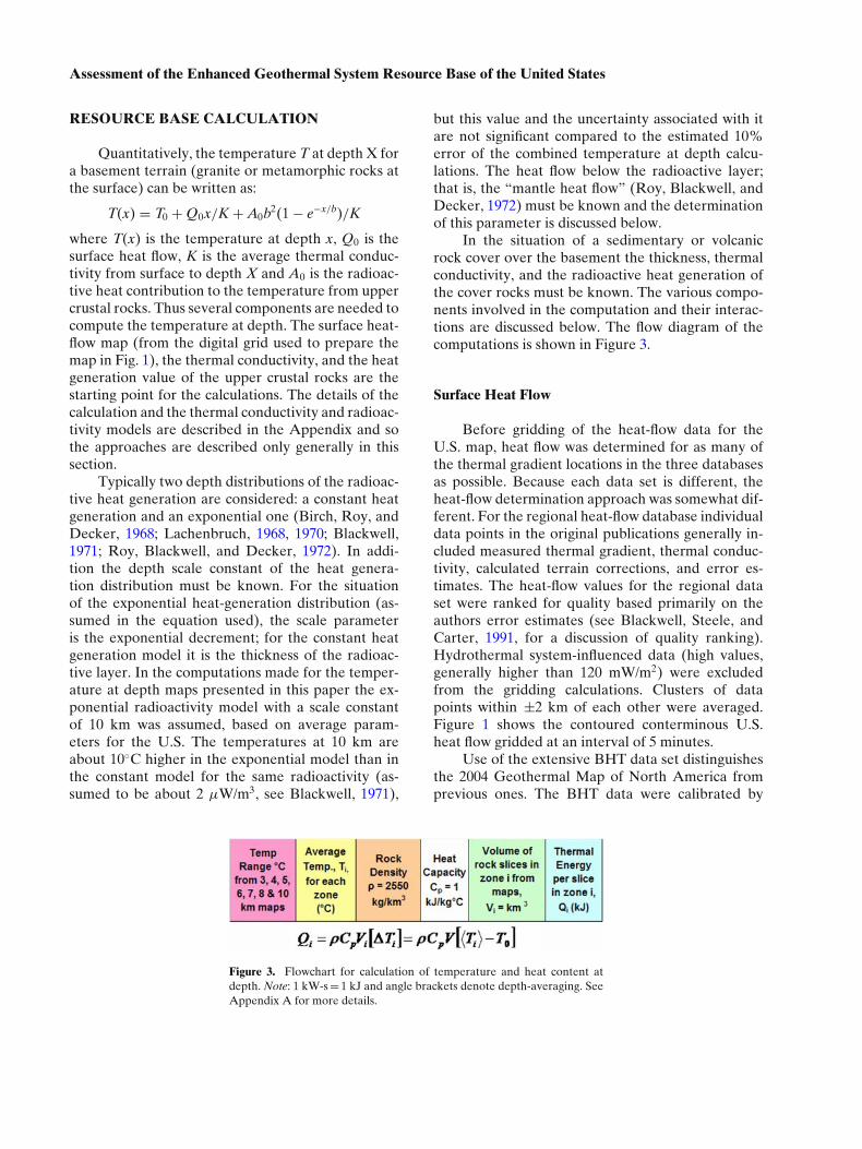
In the situation of a sedimentary or volcanicrock cover over the basement the thickness, thermalconductivity, and the radioactive heat generation ofthe cover rocks must be known. The various compo-nents involved in the computation and their interac-tions are discussed below. The flow diagram of thecomputations is shown in Figure 3.

Surface Heat Flow

Before gridding of the heat-flow data for theU.S. map, heat flow was determined for as many ofthe thermal gradient locations in the three databasesas possible. Because each data set is different, theheat-flow determination approach was somewhat dif-ferent. For the regional heat-flow database individualdata points in the original publications generally in-cluded measured thermal gradient, thermal conduc-tivity, calculated terrain corrections, and error es-timates. The heat-flow values for the regional dataset were ranked for quality based primarily on theauthors error estimates (see Blackwell, Steele, andCarter, 1991, for a discussion of quality ranking).Hydrothermal system-influenced data (high values,generally higher than 120 mW/m2) were excludedfrom the gridding calculations. Clusters of datapoints within ±2 km of each other were averaged.Figure 1 shows the contoured conterminous U.S.heat flow gridded at an interval of 5 minutes.

Use of the extensive BHT data set distinguishesthe 2004 Geothermal Map of North America fromprevious ones. The BHT data were calibrated by

Figure 3. Flowchart for calculation of temperature and heat content atdepth. Note: 1 kW-s = 1 kJ and angle brackets denote depth-averaging. SeeAppendix A for more details.

Blackwell, Negraru, and Richards

comparison to a series of precision temperature mea-surements made in hydrocarbon wells in thermalequilibrium and a BHT error was thus established(Blackwell and Richards, 2004b). Corrected temper-atures up to a maximum depth of 3,000 m were used(4,000 m in southern Louisiana). The basic correctionwas similar to the AAPG BHT correction with mod-ifications as proposed by Harrison and others (1983).A secondary correction that is a function of the localgeothermal gradient was then applied so that a biasassociated with the average geothermal gradient inthe well was removed. This correction was checkedagainst approximately 30 sites in the U.S. with ac-curate thermal logs. We believe the correction forthe average gradient of a group of wells is accurateto about ±8◦C at 100◦C (corresponding to a gradi-ent error of about 10%), based on comparison ofthe results to the measured equilibrium temperaturelogs.

Although there are BHT data in some areas todepths of 6 km, the maximum depth used for the cor-rection was limited to BHT’s from depths of less than4 km because of limited information on the drillingeffect for wells deeper than 4 km, and a lack of cali-bration wells at those depths. However, for geother-mal resource potential purposes, the BHT data canbe used qualitatively in places where measurementsare at 4 to 6 km depths. These additional dataimprove the definition of areas that qualify for fur-ther EGS evaluation.

Generalized thermal conductivity models forspecific geographic areas of several sedimentarybasins were used to compute the heat flow associatedwith the BHT gradients. The results were checkedagainst conventional heat-flow measurements in thesame regions for general agreement. With the newanalysis of the BHT data (Blackwell and Richards,2004c) there is a higher confidence level in the inter-preted BHT heat-flow values.

Data from the Western Geothermal Databasealso were used to prepare the heat-flow contour map.The heat-flow measurements were derived fromthermal gradient exploration wells drilled primar-ily for geothermal resource exploration in the west-ern U.S., in most situations during the late 1970’sand 1980’s. The raw thermal data were processedto calculate heat flow where there was sufficient in-formation. There are site/well specific thermal con-ductivity data for about 50% of the sites. Estimatedthermal conductivity was used for other sites (seenext section).

Thermal Conductivity

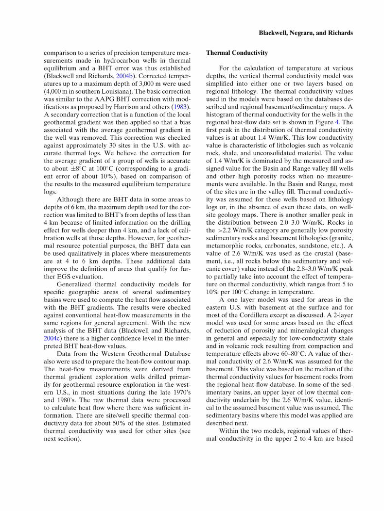
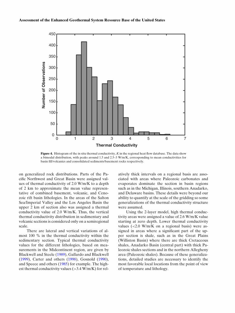
For the calculation of temperature at variousdepths, the vertical thermal conductivity model wassimplified into either one or two layers based onregional lithology. The thermal conductivity valuesused in the models were based on the databases de-scribed and regional basement/sedimentary maps. Ahistogram of thermal conductivity for the wells in theregional heat-flow data set is shown in Figure 4. Thefirst peak in the distribution of thermal conductivityvalues is at about 1.4 W/m/K. This low conductivityvalue is characteristic of lithologies such as volcanicrock, shale, and unconsolidated material. The valueof 1.4 W/m/K is dominated by the measured and as-signed value for the Basin and Range valley fill wellsand other high porosity rocks when no measure-ments were available. In the Basin and Range, mostof the sites are in the valley fill. Thermal conductiv-ity was assumed for these wells based on lithologylogs or, in the absence of even these data, on well-site geology maps. There is another smaller peak inthe distribution between 2.0–3.0 W/m/K. Rocks inthe >2.2 W/m/K category are generally low porositysedimentary rocks and basement lithologies (granite,metamorphic rocks, carbonates, sandstone, etc.). Avalue of 2.6 W/m/K was used as the crustal (base-ment, i.e., all rocks below the sedimentary and vol-canic cover) value instead of the 2.8–3.0 W/m/K peakto partially take into account the effect of tempera-ture on thermal conductivity, which ranges from 5 to10% per 100◦C change in temperature.

A one layer model was used for areas in theeastern U.S. with basement at the surface and formost of the Cordillera except as discussed. A 2-layermodel was used for some areas based on the effectof reduction of porosity and mineralogical changesin general and especially for low-conductivity shaleand in volcanic rock resulting from compaction andtemperature effects above 60–80◦C. A value of ther-mal conductivity of 2.6 W/m/K was assumed for thebasement. This value was based on the median of thethermal conductivity values for basement rocks fromthe regional heat-flow database. In some of the sed-imentary basins, an upper layer of low thermal con-ductivity underlain by the 2.6 W/m/K value, identi-cal to the assumed basement value was assumed. Thesedimentary basins where this model was applied aredescribed next.

Within the two models, regional values of ther-mal conductivity in the upper 2 to 4 km are based

Assessment of the Enhanced Geothermal System Resource Base of the United States

0 1 2 3 4 5 6 70

50

100

150

200

250

300

350

400

450

Nu

mb

er o

f O

bse

rvat

ion

s

Thermal Conductivity

Figure 4. Histogram of the in situ thermal conductivity, K in the regional heat flow database. The data showa bimodal distribution, with peaks around 1.5 and 2.5–3 W/m/K, corresponding to mean conductivities forbasin fill/volcanics and consolidated sediments/basement rocks respectively.

on generalized rock distributions. Parts of the Pa-cific Northwest and Great Basin were assigned val-ues of thermal conductivity of 2.0 W/m/K to a depthof 2 km to approximate the mean value represen-tative of combined basement, volcanic, and Ceno-zoic rift basin lithologies. In the areas of the SaltonSea/Imperial Valley and the Los Angeles Basin theupper 2 km of section also was assigned a thermalconductivity value of 2.0 W/m/K. Thus, the verticalthermal conductivity distribution in sedimentary andvolcanic sections is considered only on a semiregionalscale.

There are lateral and vertical variations of al-most 100 % in the thermal conductivity within thesedimentary section. Typical thermal conductivityvalues for the different lithologies, based on mea-surements in the Midcontinent region, are given byBlackwell and Steele (1989), Gallardo and Blackwell(1999), Carter and others (1998), Gosnold (1990),and Speece and others (1985) for example. The high-est thermal conductivity values (>3.4 W/m/K) for rel-

atively thick intervals on a regional basis are asso-ciated with areas where Paleozoic carbonates andevaporates dominate the section in basin regionssuch as in the Michigan, Illinois, southern Anadarko,and Delaware basins. These details were beyond ourability to quantify at the scale of the gridding so somegeneralizations of the thermal conductivity structurewere assumed.

Using the 2-layer model, high thermal conduc-tivity areas were assigned a value of 2.6 W/m/K valuestarting at zero depth. Lower thermal conductivityvalues (<2.0 W/m/K on a regional basis) were as-signed in areas where a significant part of the up-per section is shale, such as in the Great Plains(Williston Basin) where there are thick Cretaceousshales, Anadarko Basin (central part) with thick Pa-leozoic shales sections and in the northern Alleghenyarea (Paleozoic shales). Because of these generaliza-tions, detailed studies are necessary to identify themost favorable local locations from the point of viewof temperature and lithology.

Blackwell, Negraru, and Richards

Geothermal Gradients

By dividing the thermal conductivity into theheat flow, mean gradients can be obtained. How-ever, the approach used here to compute the spe-cific depth temperatures does not require directly theuse of geothermal gradients, although in some pub-lications they are preferred because they are easierto understand than the heat flow. We start with theheat-flow value because in a single well the gradientscan differ by as much as a factor of five or more de-pending on the thermal conductivity of the rocks, re-sulting in a lithologic (depth of measurement) bias.The gradients computed from the heat-flow map aresmoother, appropriate with the scale of this study,and more regionally characteristic than some ex-isting gradient compilations (Kron and Stix, 1982;Nathenson and Guffanti, 1980). On a regional ba-sis those gradients can range from 15◦C/km to morethan 50◦C/km, excluding of course the high gradientsin hydrothermal areas.

Sediment Thickness

A map of the thickness of sedimentary cover wasprepared by digitizing the elevation of the basementmap published by the AAPG (1978). The basementelevation was converted to thickness by subtractingits value from the digital topography. The result-ing map is illustrated in Figure 5. Sediment thick-ness is highly variable from place to place in thetectonic regions in the Western U.S. and, for this rea-son, most of the areas of deformation in the WesternU.S. do not have basement contours on the AAPGmap. Because of the complexity and lack of data, thesediment/basement division in the Cordillera is notshown, with the exception of the Colorado Plateau(eastern Utah and western Colorado), the MiddleRocky Mountains (Wyoming), and the Great Val-ley of California. The area of most uncertainty is theNorthern Rocky Mountain/Sevier thrust belt of theCordillera. In that area basement thermal conductiv-ity was assumed.

Figure 5. Sediment thickness map (in km, modified from AAPG Basement Map of North America, 1978). The 4 km depth contour isoutlined with a bold black line. The low conductivity areas in the western U.S. are shown as patterned areas.

Assessment of the Enhanced Geothermal System Resource Base of the United States

In the Basin and Range and the Southern andMiddle Rocky Mountains there are smaller, but lo-cally deep basins filled with low thermal conductivitymaterial. The scale of this study is such that these ar-eas are not examined in detail and considerable vari-ations are possible in those regions, both hotter andcolder than predicted. A more detailed map of theGreat Basin and its margins was prepared at a grid-ding interval of 2.5′ for regional resource evaluationpurposes (Coolbaugh and others, 2005a, 2005b).

The map in Figure 5 indicates regional scale ar-eas that might be of interest for EGS development inthe sediment section and areas of interest for base-ment EGS. East of the Rocky Mountains, with theexception of the Anadarko Basin, the Gulf Coast,and the eastern edge of the Allegheny Basin, sedi-mentary thickness does not exceed 4 km except inlocalized regions. Thus east of the Rocky Mountainsand outside the areas identified by the heavy lines onFigure 5, EGS (or other geothermal) developmentwould be in basement settings.

The sediment thickness influences the temper-ature calculations in two ways. First, as previouslydiscussed in the conductivity section, the sedimen-tary rocks have in general lower conductivity thanmost of the basement rocks, and the geothermal gra-dients will be higher. The second effect is becauseof the radioactive heat distribution, and is discussedin the next section.

Tectonic and Radioactive Componentsof Heat Flow

The heat flow at the surface is composed of twomain components that may of course be perturbed bylocal effects; that is, the heat generated by radioac-tive elements in the crust and the tectonic compo-nent of heat flow that comes from the interior of theEarth. The radioactive component ranges from 0 tomore than 100 mW/m2 with a typical value of about25 mW/m2. The characteristic depth of the radioele-ments (U, Th, and K) in the crust averages between7 to 10 km (Roy, Blackwell, and Decker, 1972) sothat most of the variation in heat flow caused by ra-dioactivity variations is above that depth. This com-ponent can be large and locally is variable and thusthere can be areas of high heat flow even in areas thatare considered stable continent. For example in theWhite Mountains in New Hampshire the heat flow isas high as 100 mW/m2 because of the extreme nat-ural radioactivity of the granite there (Birch, Roy,and Decker, 1968). Also there is an area of high heat

flow and basement radioactivity in northern Illinois(Roy, Rahman, and Blackwell, 1989). In contrastthe surface heat flow is only 30 mW/m2 in parts ofthe Adirondack Mountains because the upper crustalrocks there have small radioelement content.

In the analysis of temperatures to 10 km, thecomponent of heat flow not related to crustal ra-dioactivity must be known. Fortunately the discoveryof the linear heat flow heat generation relationshipallows a quantification of this parameter. For the ma-jority of the area, two different heat-flow values wereused: 60 mW/m2 for the high heat flow regions in thewest and 30 mW/m2 for most of the rest of the maparea (see Roy, Blackwell, and Decker, 1972; Morganand Gosnold, 1989). The area of high mantle heatflow is shown as the shaded area in Figure 6. The highmantle heat flow is a result of the plate tectonic ac-tivity (subduction) that has occurred along the westcoast of North America over the past 100 Ma. Partof the Cascade Range in the Pacific Northwest andpart of the Snake River Plain were assigned man-tle heat flow values of 80 mW/m2 because they areassociated directly with geologically young volcan-ism (Brott, Blackwell, and Mitchell, 1978; Blackwelland others, 1990a, 1990b). Finally part of the GreatValley/Sierra Nevada Mountains areas were given amantle heat flow of 20 mW/m2 compatible with theouter arc tectonic setting in those areas (see Morganand Gosnold, 1989; Blackwell, Steele, and Carter,1991). Transitions in heat flow between these differ-ent areas are generally sharp on the scale of the mapbut are difficult to recognize in some locations be-cause of the variable heat flow resulting from the up-per crustal effects. At the maximum depth of 10 kmused in this study the relative effects of heat produc-tion and mantle heat flow on temperature are similar,but as deeper and deeper depths are considered themantle heat flow factor become dominant.

The radioactivity value of the basement is highlyvariable and has only been measured in a few places.To determine the average radioactivity value appro-priate at each calculation node is impractical. There-fore the Q-A model was assumed to hold and the ra-dioactivity value for each node was assumed to bethe surface heat flow (Q0) minus the mantle (m) heatflow (Qm) divided by 10 km. Thus at each basementnode the surface heat flow is assumed to be exactlyon the Q-A line with a slope of 10 km and an inter-cept given by the mantle heat-flow value in Figure 6.

In general the radioactive heat generation is sig-nificant to a depth of 10 to 20 km. As modeled itwas assumed to decay exponentially with depth in

Blackwell, Negraru, and Richards

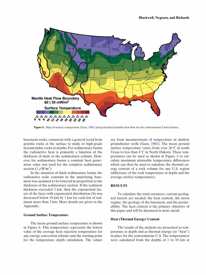
Figure 6. Map of surface temperature (Gass, 1982) and generalized mantle heat flow for the conterminous United States.

basement rocks, consistent with a general trend fromgranitic rocks at the surface to mafic or high-grademetamorphic rocks at depths. For sedimentary basinsthe radioactive heat is primarily a function of thethickness of shale in the sedimentary column. How-ever for sedimentary basins a constant heat gener-ation value was used for the complete sedimentarysection (1 µW/m3).

In the situation of thick sedimentary basins theradioactive scale constant in the underlying base-ment was assumed to be lowered in proportion to thethickness of the sedimentary section. If the sedimentthickness exceeded 3 km, then the exponential fac-tor of the layer with exponential distribution (b) wasdecreased below 10 km by 1 km for each km of sed-iment more than 3 km. More details are given in theAppendix.

Ground Surface Temperature

The mean ground surface temperature is shownin Figure 6. This temperature represents the lowestvalue of the average heat rejection temperature forany energy conversion scheme and the starting pointfor the temperature depth calculation. The values

are from measurements of temperature in shallowgroundwater wells (Gass, 1982). The mean groundsurface temperature varies from over 26◦C in southTexas to less than 4◦C in North Dakota. These tem-peratures can be used as shown in Figure 3 to cal-culate maximum attainable temperature differenceswhich can then be used to calculate the thermal en-ergy content of a rock volume for any U.S. region(difference of the rock temperature at depth and theaverage surface temperature).

RESULTS

To calculate the total resources, various geolog-ical factors are needed: the heat content, the stressregime, the geology of the basement, and the perme-ability. The heat content is the primary objective ofthis paper and will be discussed in more detail.

Heat (Thermal Energy) Content

The results of the analysis are presented as tem-perature at depth and as thermal energy (or “heat”)in place for the conterminous U.S. The temperatureswere calculated from the depths of 1 to 10 km at

Assessment of the Enhanced Geothermal System Resource Base of the United States

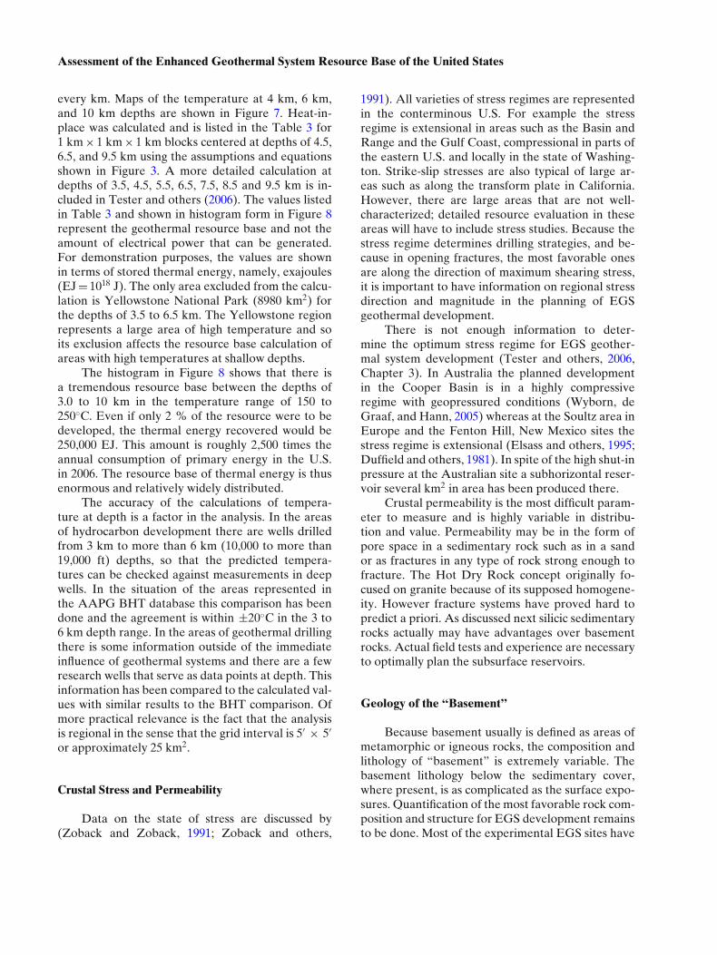
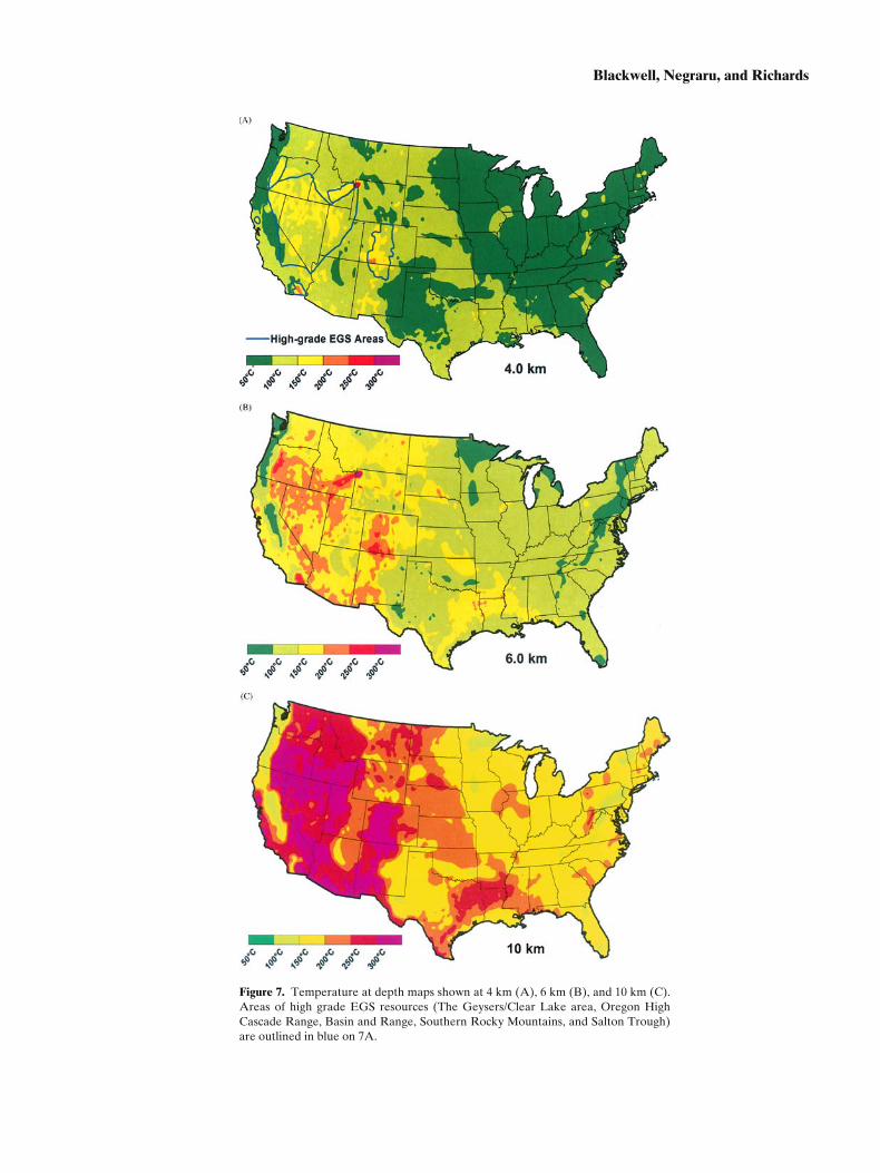
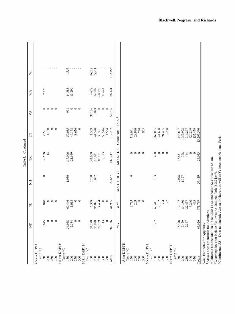
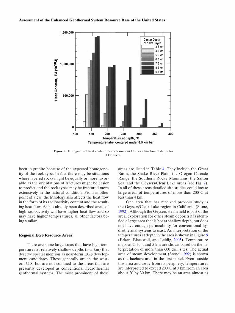
every km. Maps of the temperature at 4 km, 6 km,and 10 km depths are shown in Figure 7. Heat-in-place was calculated and is listed in the Table 3 for1 km × 1 km × 1 km blocks centered at depths of 4.5,6.5, and 9.5 km using the assumptions and equationsshown in Figure 3. A more detailed calculation atdepths of 3.5, 4.5, 5.5, 6.5, 7.5, 8.5 and 9.5 km is in-cluded in Tester and others (2006). The values listedin Table 3 and shown in histogram form in Figure 8represent the geothermal resource base and not theamount of electrical power that can be generated.For demonstration purposes, the values are shownin terms of stored thermal energy, namely, exajoules(EJ = 1018 J). The only area excluded from the calcu-lation is Yellowstone National Park (8980 km2) forthe depths of 3.5 to 6.5 km. The Yellowstone regionrepresents a large area of high temperature and soits exclusion affects the resource base calculation ofareas with high temperatures at shallow depths.

The histogram in Figure 8 shows that there isa tremendous resource base between the depths of3.0 to 10 km in the temperature range of 150 to250◦C. Even if only 2 % of the resource were to bedeveloped, the thermal energy recovered would be250,000 EJ. This amount is roughly 2,500 times theannual consumption of primary energy in the U.S.in 2006. The resource base of thermal energy is thusenormous and relatively widely distributed.

The accuracy of the calculations of tempera-ture at depth is a factor in the analysis. In the areasof hydrocarbon development there are wells drilledfrom 3 km to more than 6 km (10,000 to more than19,000 ft) depths, so that the predicted tempera-tures can be checked against measurements in deepwells. In the situation of the areas represented inthe AAPG BHT database this comparison has beendone and the agreement is within ±20◦C in the 3 to6 km depth range. In the areas of geothermal drillingthere is some information outside of the immediateinfluence of geothermal systems and there are a fewresearch wells that serve as data points at depth. Thisinformation has been compared to the calculated val-ues with similar results to the BHT comparison. Ofmore practical relevance is the fact that the analysisis regional in the sense that the grid interval is 5′ × 5′

or approximately 25 km2.

Crustal Stress and Permeability

Data on the state of stress are discussed by(Zoback and Zoback, 1991; Zoback and others,

1991). All varieties of stress regimes are representedin the conterminous U.S. For example the stressregime is extensional in areas such as the Basin andRange and the Gulf Coast, compressional in parts ofthe eastern U.S. and locally in the state of Washing-ton. Strike-slip stresses are also typical of large ar-eas such as along the transform plate in California.However, there are large areas that are not well-characterized; detailed resource evaluation in theseareas will have to include stress studies. Because thestress regime determines drilling strategies, and be-cause in opening fractures, the most favorable onesare along the direction of maximum shearing stress,it is important to have information on regional stressdirection and magnitude in the planning of EGSgeothermal development.

There is not enough information to deter-mine the optimum stress regime for EGS geother-mal system development (Tester and others, 2006,Chapter 3). In Australia the planned developmentin the Cooper Basin is in a highly compressiveregime with geopressured conditions (Wyborn, deGraaf, and Hann, 2005) whereas at the Soultz area inEurope and the Fenton Hill, New Mexico sites thestress regime is extensional (Elsass and others, 1995;Duffield and others, 1981). In spite of the high shut-inpressure at the Australian site a subhorizontal reser-voir several km2 in area has been produced there.

Crustal permeability is the most difficult param-eter to measure and is highly variable in distribu-tion and value. Permeability may be in the form ofpore space in a sedimentary rock such as in a sandor as fractures in any type of rock strong enough tofracture. The Hot Dry Rock concept originally fo-cused on granite because of its supposed homogene-ity. However fracture systems have proved hard topredict a priori. As discussed next silicic sedimentaryrocks actually may have advantages over basementrocks. Actual field tests and experience are necessaryto optimally plan the subsurface reservoirs.

Geology of the “Basement”

Because basement usually is defined as areas ofmetamorphic or igneous rocks, the composition andlithology of “basement” is extremely variable. Thebasement lithology below the sedimentary cover,where present, is as complicated as the surface expo-sures. Quantification of the most favorable rock com-position and structure for EGS development remainsto be done. Most of the experimental EGS sites have

Blackwell, Negraru, and Richards

Figure 7. Temperature at depth maps shown at 4 km (A), 6 km (B), and 10 km (C).Areas of high grade EGS resources (The Geysers/Clear Lake area, Oregon HighCascade Range, Basin and Range, Southern Rocky Mountains, and Salton Trough)are outlined in blue on 7A.

Assessment of the Enhanced Geothermal System Resource Base of the United StatesT

able

3.H

eati

nP

lace

(Exa

joul

es=

1018

J)

AK

1A

LA

RA

ZC

A2

CO

FL

GA

IAID

IL

4.5

kmD

EP

TH

Tem

p◦ C

150

39,5

8834

6,36

149

,886

53,0

6845

,890

00

036

,008

020

00

00

4,73

48,

413

00

07,

218

025

00

00

407

00

011

20

300

00

079

60

00

00

6.5

kmD

EP

TH

Tem

p◦ C

150

361,

688

9,14

820

,725

52,3

3554

,243

54,6

674,

339

9510

,729

35,2

572,

005

200

187,

722

606,

373

74,3

0570

,941

51,1

702

00

53,8

7525

00

047

39,

186

24,0

290

00

19,5

1030

00

00

176

1,07

70

00

359

10km

DE

PT

HT

emp

◦ C15

025

,073

42,6

4326

,260

9,92

236

,089

4,31

648

,062

57,4

8543

,425

040

,906

200

122,

877

16,3

1725

,125

39,4

6731

,336

47,1

316,

019

3,57

116

,970

2,34

626

,368

250

520,

597

111

18,6

3564

,525

73,8

1245

,614

50

071

,702

300

199,

506

029

680

,190

77,3

0757

,944

00

052

,488

350

00

1,50

012

,844

33,2

510

00

28,1

38T

otal

s3,

203,

825

115,

655

229,

089

777,

471

888,

460

798,

437

60,4

9458

,424

126,

100

673,

966

186,

123

INK

SK

YL

AM

EM

IM

NM

OM

SM

TN

C

4.5

kmD

EP

TH

Tem

p◦ C

150

00

011

,455

00

00

1,51

28,

373

020

00

00

00

00

025

00

00

00

00

030

00

00

00

00

06.

5km

DE

PT

HT

emp

◦ C15

00

57,5

560

15,2

8078

50

084

31,8

0712

3,86

02,

036

200

00

11,0

280

00

01,

158

13,2

650

250

00

00

00

250

300

00

00

00

010

kmD

EP

TH

Tem

p◦ C

150

39,0

0318

,783

42,8

9720

,773

26,7

5756

,156

66,2

1574

,394

14,6

2122

,297

45,8

3420

00

94,3

2641

10,1

479,

379

00

2,36

638

,876

72,7

616,

103

250

00

27,9

430

00

09,

192

128,

534

3330

00

00

00

050

2,80

30

350

00

00

00

520

Tot

als

95,9

5634

5,68

988

,100

201,

019

99,1

2644

,852

35,7

8917

6,68

420

9,52

884

0,31

271

,437

Blackwell, Negraru, and RichardsT

able

3.C

onti

nued

ND

NE

NH

TX

UT

VA

WA

WI

4.5

kmD

EP

TH

Tem

p◦ C

150

3,84

584

80

32,5

2836

,521

09,

796

020

00

014

1,16

00

025

00

00

00

300

00

00

06.

5km

DE

PT

HT

emp

◦ C15

036

,938

60,4

461,

050

117,

096

50,0

8599

144

,388

1,73

320

02,

534

1,01

821

,659

44,1

780

13,2

900

250

00

8,62

60

030

00

00

00

10km

DE

PT

HT

emp

◦ C15

034

,198

6,35

86,

780

144,

600

1,53

930

,176

4,67

856

,012

200

36,9

7896

,021

3,03

211

3,02

144

,520

3,84

914

,189

5,81

125

022

,759

4,40

486

,151

38,3

910

60,1

950

300

130

2,72

350

,546

011

,641

035

00

011

,554

00

Tot

als

289,

756

341,

935

22,6

571,

068,

217

612,

202

50,7

9633

8,32

410

2,15

5

WV

WY

3M

AC

TR

IV

TM

DN

JD

EC

onti

nent

alU

.S.A

.4

4.5

kmD

EP

TH

Tem

p◦ C

150

6,79

50

051

8,04

120

020

30

29,9

3025

08

073

430

00

096

56.

5km

DE

PT

HT

emp

◦ C15

03,

367

68,4

1118

346

81,

062,

065

200

7,13

20

641,

638

250

334

094

,405

300

177

02,

268

10km

DE

PT

HT

emp

◦ C15

015

,476

19,1

0719

,078

13,8

511,

446,

607

200

7,47

984

,380

1,37

772

81,

057,

978

250

2,37

727

,437

464

914,

277

300

3,24

00

620,

849

350

493

013

2,47

9T

otal

s63

,626

471,

799

37,4

1923

,033

13,2

67,3

70

Not

e.F

ootn

otes

for

App

endi

x1 A

lask

ado

esno

tinc

lude

the

Ale

utia

ns.

2 Cal

ifor

nia

has

the

addi

tion

ofth

eC

lear

Lak

ean

dSa

lton

Sea

area

sfo

r4.

5km

.3 W

yom

ing

does

noti

nclu

deY

ello

wst

one

Nat

iona

lPar

k(8

987

km2 ).

4 Con

tine

ntal

U.S

.-D

oes

noti

nclu

deA

lask

aor

Haw

aii,

asw

ella

sY

ello

wst

one

Nat

iona

lPar

k.

Assessment of the Enhanced Geothermal System Resource Base of the United States

Figure 8. Histograms of heat content for conterminous U.S. as a function of depth for1 km slices.

been in granite because of the expected homogene-ity of the rock type. In fact there may be situationswhere layered rocks might be equally or more favor-able as the orientations of fractures might be easierto predict and the rock types may be fractured moreextensively in the natural condition. From anotherpoint of view, the lithology also affects the heat flowin the form of its radioactivity content and the result-ing heat flow. As has already been described areas ofhigh radioactivity will have higher heat flow and somay have higher temperatures, all other factors be-ing similar.

Regional EGS Resource Areas

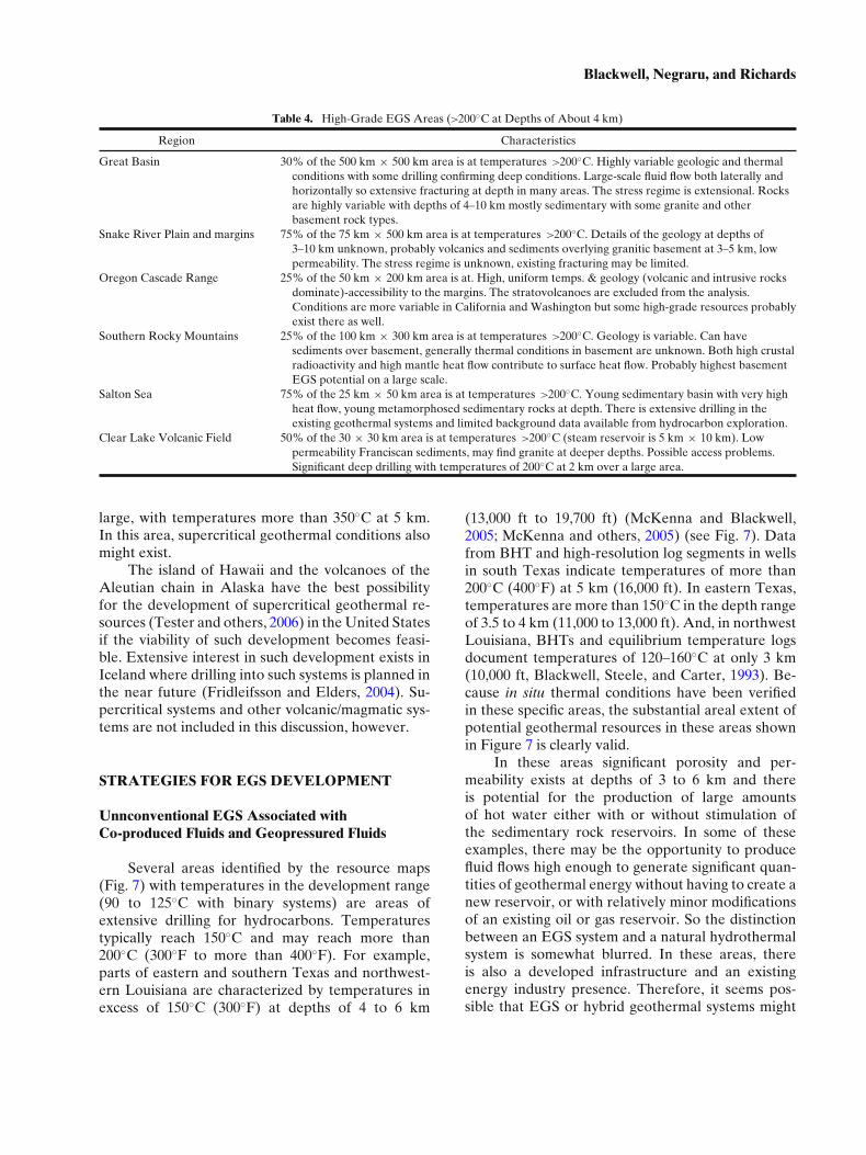
There are some large areas that have high tem-peratures at relatively shallow depths (3–5 km) thatdeserve special mention as near-term EGS develop-ment candidates. These generally are in the west-ern U.S, but are not confined to the areas that arepresently developed as conventional hydrothermalgeothermal systems. The most prominent of these

areas are listed in Table 4. They include the GreatBasin, the Snake River Plain, the Oregon CascadeRange, the Southern Rocky Mountains, the SaltonSea, and the Geysers/Clear Lake areas (see Fig. 7).In all of these areas detailed site studies could locatelarge areas of temperatures of more than 200◦C atless than 4 km.

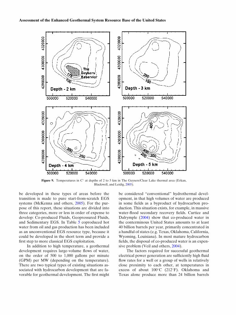
One area that has received previous study isthe Geysers/Clear Lake region in California (Stone,1992). Although the Geysers steam field is part of thearea, exploration for other steam deposits has identi-fied a large area that is hot at shallow depth, but doesnot have enough permeability for conventional hy-drothermal systems to exist. An interpretation of thetemperatures at depth in the area is shown in Figure 9(Erkan, Blackwell, and Leidig, 2005). Temperaturemaps at 2, 3, 4, and 5 km are shown based on the in-terpretation of more than 600 drill sites. The actualarea of steam development (Stone, 1992) is shownas the hachure area in the first panel. Even outsidethis area and away from its periphery, temperaturesare interpreted to exceed 200◦C at 3 km from an areaabout 20 by 30 km. There may be an area almost as

Blackwell, Negraru, and Richards

Table 4. High-Grade EGS Areas (>200◦C at Depths of About 4 km)

Region Characteristics

Great Basin 30% of the 500 km × 500 km area is at temperatures >200◦C. Highly variable geologic and thermalconditions with some drilling confirming deep conditions. Large-scale fluid flow both laterally andhorizontally so extensive fracturing at depth in many areas. The stress regime is extensional. Rocksare highly variable with depths of 4–10 km mostly sedimentary with some granite and otherbasement rock types.

Snake River Plain and margins 75% of the 75 km × 500 km area is at temperatures >200◦C. Details of the geology at depths of3–10 km unknown, probably volcanics and sediments overlying granitic basement at 3–5 km, lowpermeability. The stress regime is unknown, existing fracturing may be limited.

Oregon Cascade Range 25% of the 50 km × 200 km area is at. High, uniform temps. & geology (volcanic and intrusive rocksdominate)-accessibility to the margins. The stratovolcanoes are excluded from the analysis.Conditions are more variable in California and Washington but some high-grade resources probablyexist there as well.

Southern Rocky Mountains 25% of the 100 km × 300 km area is at temperatures >200◦C. Geology is variable. Can havesediments over basement, generally thermal conditions in basement are unknown. Both high crustalradioactivity and high mantle heat flow contribute to surface heat flow. Probably highest basementEGS potential on a large scale.

Salton Sea 75% of the 25 km × 50 km area is at temperatures >200◦C. Young sedimentary basin with very highheat flow, young metamorphosed sedimentary rocks at depth. There is extensive drilling in theexisting geothermal systems and limited background data available from hydrocarbon exploration.

Clear Lake Volcanic Field 50% of the 30 × 30 km area is at temperatures >200◦C (steam reservoir is 5 km × 10 km). Lowpermeability Franciscan sediments, may find granite at deeper depths. Possible access problems.Significant deep drilling with temperatures of 200◦C at 2 km over a large area.

large, with temperatures more than 350◦C at 5 km.In this area, supercritical geothermal conditions alsomight exist.

The island of Hawaii and the volcanoes of theAleutian chain in Alaska have the best possibilityfor the development of supercritical geothermal re-sources (Tester and others, 2006) in the United Statesif the viability of such development becomes feasi-ble. Extensive interest in such development exists inIceland where drilling into such systems is planned inthe near future (Fridleifsson and Elders, 2004). Su-percritical systems and other volcanic/magmatic sys-tems are not included in this discussion, however.

STRATEGIES FOR EGS DEVELOPMENT

Unnconventional EGS Associated withCo-produced Fluids and Geopressured Fluids

Several areas identified by the resource maps(Fig. 7) with temperatures in the development range(90 to 125◦C with binary systems) are areas ofextensive drilling for hydrocarbons. Temperaturestypically reach 150◦C and may reach more than200◦C (300◦F to more than 400◦F). For example,parts of eastern and southern Texas and northwest-ern Louisiana are characterized by temperatures inexcess of 150◦C (300◦F) at depths of 4 to 6 km

(13,000 ft to 19,700 ft) (McKenna and Blackwell,2005; McKenna and others, 2005) (see Fig. 7). Datafrom BHT and high-resolution log segments in wellsin south Texas indicate temperatures of more than200◦C (400◦F) at 5 km (16,000 ft). In eastern Texas,temperatures are more than 150◦C in the depth rangeof 3.5 to 4 km (11,000 to 13,000 ft). And, in northwestLouisiana, BHTs and equilibrium temperature logsdocument temperatures of 120–160◦C at only 3 km(10,000 ft, Blackwell, Steele, and Carter, 1993). Be-cause in situ thermal conditions have been verifiedin these specific areas, the substantial areal extent ofpotential geothermal resources in these areas shownin Figure 7 is clearly valid.

In these areas significant porosity and per-meability exists at depths of 3 to 6 km and thereis potential for the production of large amountsof hot water either with or without stimulation ofthe sedimentary rock reservoirs. In some of theseexamples, there may be the opportunity to producefluid flows high enough to generate significant quan-tities of geothermal energy without having to create anew reservoir, or with relatively minor modificationsof an existing oil or gas reservoir. So the distinctionbetween an EGS system and a natural hydrothermalsystem is somewhat blurred. In these areas, thereis also a developed infrastructure and an existingenergy industry presence. Therefore, it seems pos-sible that EGS or hybrid geothermal systems might

Assessment of the Enhanced Geothermal System Resource Base of the United States

Figure 9. Temperatures in C◦ at depths of 2 to 5 km in The Geysers/Clear Lake thermal area (Erkan,Blackwell, and Leidig, 2005).

be developed in these types of areas before thetransition is made to pure start-from-scratch EGSsystems (McKenna and others, 2005). For the pur-pose of this report, these situations are divided intothree categories, more or less in order of expense todevelop: Co-produced Fluids, Geopressured Fluids,and Sedimentary EGS. In Table 5 coproduced hotwater from oil and gas production has been includedas an unconventional EGS resource type, because itcould be developed in the short term and provide afirst step to more classical EGS exploitation.

In addition to high temperature, a geothermaldevelopment requires large-volume flows of water,on the order of 500 to 1,000 gallons per minute(GPM) per MW (depending on the temperature).There are two typical types of existing situations as-sociated with hydrocarbon development that are fa-vorable for geothermal development. The first might

be considered “conventional” hydrothermal devel-opment, in that high volumes of water are producedin some fields as a byproduct of hydrocarbon pro-duction. This situation exists, for example, in massivewater-flood secondary recovery fields. Curtice andDalrymple (2004) show that co-produced water inthe conterminous United States amounts to at least40 billion barrels per year, primarily concentrated ina handful of states (e.g. Texas, Oklahoma, California,Wyoming, Louisiana). In most mature hydrocarbonfields, the disposal of co-produced water is an expen-sive problem (Veil and others, 2004).

The factors required for successful geothermalelectrical power generation are sufficiently high fluidflow rates for a well or a group of wells in relativelyclose proximity to each other, at temperatures inexcess of about 100◦C (212◦F). Oklahoma andTexas alone produce more than 24 billion barrels

Blackwell, Negraru, and Richards

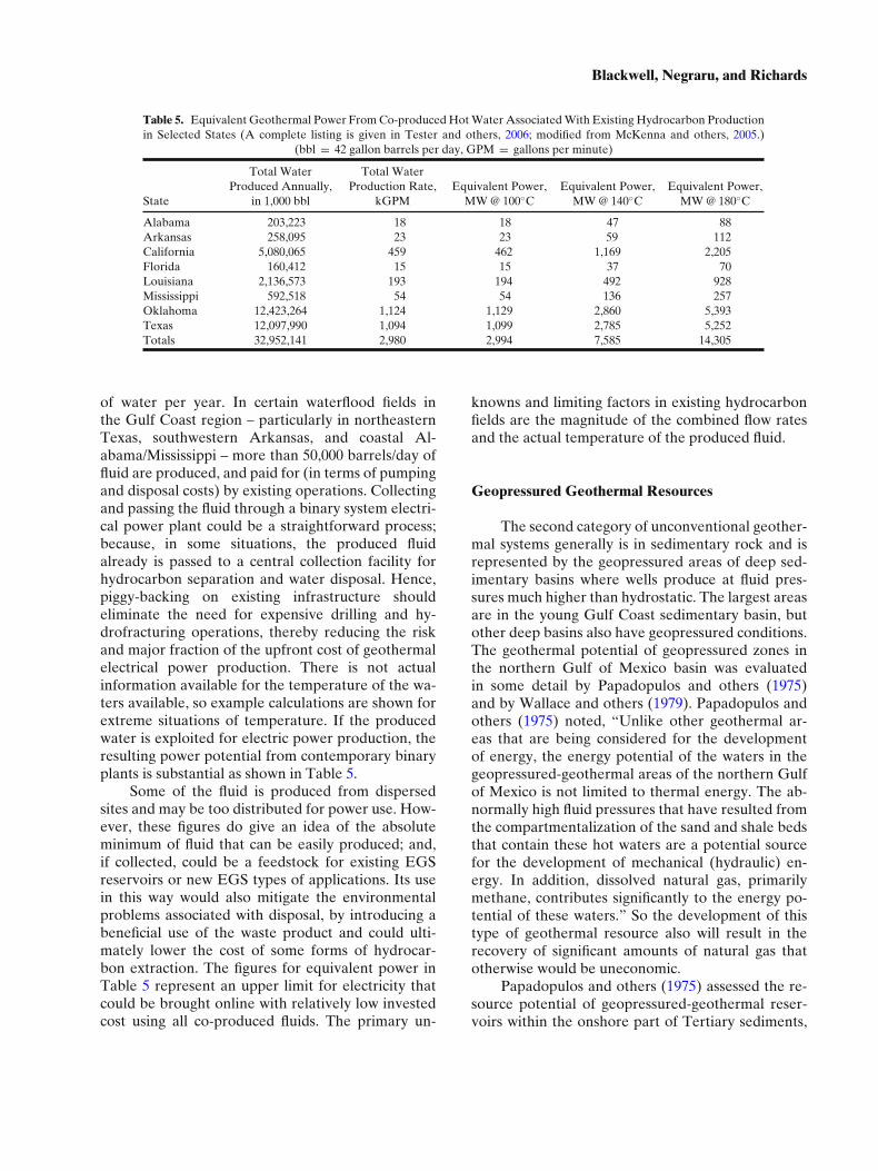
Table 5. Equivalent Geothermal Power From Co-produced Hot Water Associated With Existing Hydrocarbon Productionin Selected States (A complete listing is given in Tester and others, 2006; modified from McKenna and others, 2005.)

(bbl = 42 gallon barrels per day, GPM = gallons per minute)

State

Total WaterProduced Annually,

in 1,000 bbl

Total WaterProduction Rate,

kGPMEquivalent Power,

MW @ 100◦CEquivalent Power,

MW @ 140◦CEquivalent Power,

MW @ 180◦C

Alabama 203,223 18 18 47 88Arkansas 258,095 23 23 59 112California 5,080,065 459 462 1,169 2,205Florida 160,412 15 15 37 70Louisiana 2,136,573 193 194 492 928Mississippi 592,518 54 54 136 257Oklahoma 12,423,264 1,124 1,129 2,860 5,393Texas 12,097,990 1,094 1,099 2,785 5,252Totals 32,952,141 2,980 2,994 7,585 14,305

of water per year. In certain waterflood fields inthe Gulf Coast region – particularly in northeasternTexas, southwestern Arkansas, and coastal Al-abama/Mississippi – more than 50,000 barrels/day offluid are produced, and paid for (in terms of pumpingand disposal costs) by existing operations. Collectingand passing the fluid through a binary system electri-cal power plant could be a straightforward process;because, in some situations, the produced fluidalready is passed to a central collection facility forhydrocarbon separation and water disposal. Hence,piggy-backing on existing infrastructure shouldeliminate the need for expensive drilling and hy-drofracturing operations, thereby reducing the riskand major fraction of the upfront cost of geothermalelectrical power production. There is not actualinformation available for the temperature of the wa-ters available, so example calculations are shown forextreme situations of temperature. If the producedwater is exploited for electric power production, theresulting power potential from contemporary binaryplants is substantial as shown in Table 5.

Some of the fluid is produced from dispersedsites and may be too distributed for power use. How-ever, these figures do give an idea of the absoluteminimum of fluid that can be easily produced; and,if collected, could be a feedstock for existing EGSreservoirs or new EGS types of applications. Its usein this way would also mitigate the environmentalproblems associated with disposal, by introducing abeneficial use of the waste product and could ulti-mately lower the cost of some forms of hydrocar-bon extraction. The figures for equivalent power inTable 5 represent an upper limit for electricity thatcould be brought online with relatively low investedcost using all co-produced fluids. The primary un-

knowns and limiting factors in existing hydrocarbonfields are the magnitude of the combined flow ratesand the actual temperature of the produced fluid.

Geopressured Geothermal Resources

The second category of unconventional geother-mal systems generally is in sedimentary rock and isrepresented by the geopressured areas of deep sed-imentary basins where wells produce at fluid pres-sures much higher than hydrostatic. The largest areasare in the young Gulf Coast sedimentary basin, butother deep basins also have geopressured conditions.The geothermal potential of geopressured zones inthe northern Gulf of Mexico basin was evaluatedin some detail by Papadopulos and others (1975)and by Wallace and others (1979). Papadopulos andothers (1975) noted, “Unlike other geothermal ar-eas that are being considered for the developmentof energy, the energy potential of the waters in thegeopressured-geothermal areas of the northern Gulfof Mexico is not limited to thermal energy. The ab-normally high fluid pressures that have resulted fromthe compartmentalization of the sand and shale bedsthat contain these hot waters are a potential sourcefor the development of mechanical (hydraulic) en-ergy. In addition, dissolved natural gas, primarilymethane, contributes significantly to the energy po-tential of these waters.” So the development of thistype of geothermal resource also will result in therecovery of significant amounts of natural gas thatotherwise would be uneconomic.

Papadopulos and others (1975) assessed the re-source potential of geopressured-geothermal reser-voirs within the onshore part of Tertiary sediments,

Assessment of the Enhanced Geothermal System Resource Base of the United States

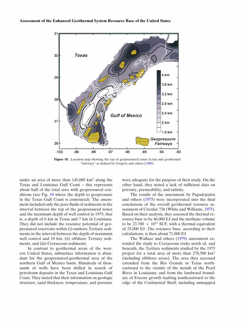
Figure 10. Location map showing the top of geopressured zones in km and geothermal“fairways” as defined by Gregory and others (1980).

under an area of more than 145,000 km2 along theTexas and Louisiana Gulf Coast – this representsabout half of the total area with geopressured con-ditions (see Fig. 10 where the depth to geopressurein the Texas Gulf Coast is contoured). The assess-ment included only the pore fluids of sediments in theinterval between the top of the geopressured zonesand the maximum depth of well control in 1975; thatis, a depth of 6 km in Texas and 7 km in Louisiana.They did not include the resource potential of geo-pressured reservoirs within (i) onshore Tertiary sedi-ments in the interval between the depth of maximumwell control and 10 km, (ii) offshore Tertiary sedi-ments, and (iii) Cretaceous sediments.

In contrast to geothermal areas of the west-ern United States, subsurface information is abun-dant for the geopressured-geothermal area of thenorthern Gulf of Mexico basin. Hundreds of thou-sands of wells have been drilled in search ofpetroleum deposits in the Texas and Louisiana GulfCoast. They stated that their information on geologicstructure, sand thickness, temperature, and pressure

were adequate for the purpose of their study. On theother hand, they noted a lack of sufficient data onporosity, permeability, and salinity.

The results of the assessment by Papadopulosand others (1975) were incorporated into the finalconclusions of the overall geothermal resource as-sessment of Circular 726 (White and Williams, 1975).Based on their analysis, they assessed the thermal re-source base to be 46,000 EJ and the methane volumeto be 23,700 × 1012 SCF, with a thermal equivalentof 25,000 EJ. The resource base, according to theircalculations, is then about 71,000 EJ.

The Wallace and others (1979) assessment ex-tended the study to Cretaceous rocks north of, andbeneath, the Tertiary sediments studied by the 1975project for a total area of more than 278,500 km2

(including offshore areas). The area they accessedextended from the Rio Grande in Texas north-eastward to the vicinity of the mouth of the PearlRiver in Louisiana; and from the landward bound-ary of Eocene growth faulting southeastward to theedge of the Continental Shelf, including unmapped

Blackwell, Negraru, and Richards

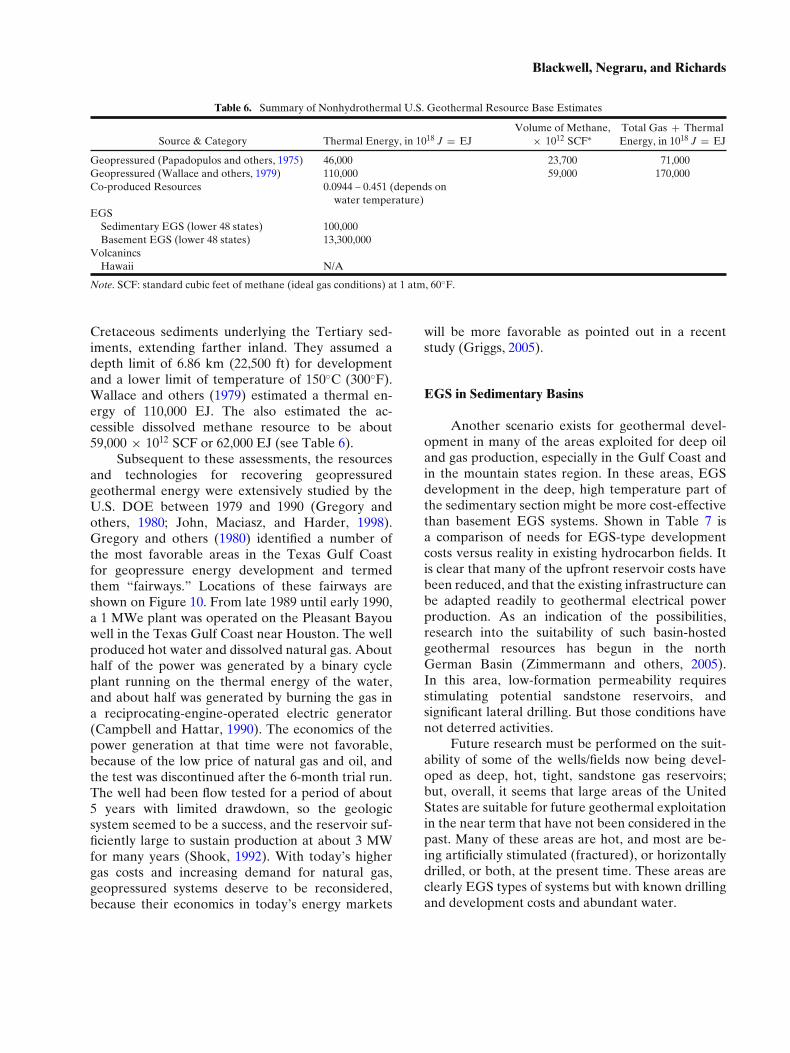
Table 6. Summary of Nonhydrothermal U.S. Geothermal Resource Base Estimates

Source & Category Thermal Energy, in 1018 J = EJVolume of Methane,

× 1012 SCF∗Total Gas + ThermalEnergy, in 1018 J = EJ

Geopressured (Papadopulos and others, 1975) 46,000 23,700 71,000Geopressured (Wallace and others, 1979) 110,000 59,000 170,000Co-produced Resources 0.0944 – 0.451 (depends on

water temperature)EGS

Sedimentary EGS (lower 48 states) 100,000Basement EGS (lower 48 states) 13,300,000

VolcanincsHawaii N/A

Note. SCF: standard cubic feet of methane (ideal gas conditions) at 1 atm, 60◦F.

Cretaceous sediments underlying the Tertiary sed-iments, extending farther inland. They assumed adepth limit of 6.86 km (22,500 ft) for developmentand a lower limit of temperature of 150◦C (300◦F).Wallace and others (1979) estimated a thermal en-ergy of 110,000 EJ. The also estimated the ac-cessible dissolved methane resource to be about59,000 × 1012 SCF or 62,000 EJ (see Table 6).

Subsequent to these assessments, the resourcesand technologies for recovering geopressuredgeothermal energy were extensively studied by theU.S. DOE between 1979 and 1990 (Gregory andothers, 1980; John, Maciasz, and Harder, 1998).Gregory and others (1980) identified a number ofthe most favorable areas in the Texas Gulf Coastfor geopressure energy development and termedthem “fairways.” Locations of these fairways areshown on Figure 10. From late 1989 until early 1990,a 1 MWe plant was operated on the Pleasant Bayouwell in the Texas Gulf Coast near Houston. The wellproduced hot water and dissolved natural gas. Abouthalf of the power was generated by a binary cycleplant running on the thermal energy of the water,and about half was generated by burning the gas ina reciprocating-engine-operated electric generator(Campbell and Hattar, 1990). The economics of thepower generation at that time were not favorable,because of the low price of natural gas and oil, andthe test was discontinued after the 6-month trial run.The well had been flow tested for a period of about5 years with limited drawdown, so the geologicsystem seemed to be a success, and the reservoir suf-ficiently large to sustain production at about 3 MWfor many years (Shook, 1992). With today’s highergas costs and increasing demand for natural gas,geopressured systems deserve to be reconsidered,because their economics in today’s energy markets

will be more favorable as pointed out in a recentstudy (Griggs, 2005).

EGS in Sedimentary Basins

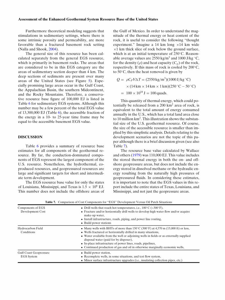
Another scenario exists for geothermal devel-opment in many of the areas exploited for deep oiland gas production, especially in the Gulf Coast andin the mountain states region. In these areas, EGSdevelopment in the deep, high temperature part ofthe sedimentary section might be more cost-effectivethan basement EGS systems. Shown in Table 7 isa comparison of needs for EGS-type developmentcosts versus reality in existing hydrocarbon fields. Itis clear that many of the upfront reservoir costs havebeen reduced, and that the existing infrastructure canbe adapted readily to geothermal electrical powerproduction. As an indication of the possibilities,research into the suitability of such basin-hostedgeothermal resources has begun in the northGerman Basin (Zimmermann and others, 2005).In this area, low-formation permeability requiresstimulating potential sandstone reservoirs, andsignificant lateral drilling. But those conditions havenot deterred activities.

Future research must be performed on the suit-ability of some of the wells/fields now being devel-oped as deep, hot, tight, sandstone gas reservoirs;but, overall, it seems that large areas of the UnitedStates are suitable for future geothermal exploitationin the near term that have not been considered in thepast. Many of these areas are hot, and most are be-ing artificially stimulated (fractured), or horizontallydrilled, or both, at the present time. These areas areclearly EGS types of systems but with known drillingand development costs and abundant water.

Assessment of the Enhanced Geothermal System Resource Base of the United States

Furthermore theoretical modeling suggests thatstimulations in sedimentary settings, where there issome intrinsic porosity and permeability, are morefavorable than a fractured basement rock setting(Nalla and Shook, 2004).

The general size of this resource has been cal-culated separately from the general EGS resource,which is primarily in basement rocks. The areas thatare considered to be in this EGS category are theareas of sedimentary section deeper than 4 km. Thedeep sections of sediments are present over manyareas of the United States (see Figure 5). Espe-cially promising large areas occur in the Gulf Coast,the Appalachian Basin, the southern Midcontinent,and the Rocky Mountains. Therefore, a conserva-tive resource base figure of 100,000 EJ is listed inTable 6 for sedimentary EGS systems. Although thisnumber may be a few percent of the total EGS valueof 13,300,000 EJ (Table 6), the accessible fraction ofthe energy in a 10- to 25-year time frame may beequal to the accessible basement EGS value.

DISCUSSION

Table 6 provides a summary of resource baseestimates for all components of the geothermal re-source. By far, the conduction-dominated compo-nents of EGS represent the largest component of theU.S. resource. Nonetheless, the hydrothermal, co-produced resources, and geopressured resources arelarge and significant targets for short and intermedi-ate term development.

The EGS resource base value for only the statesof Louisiana, Mississippi, and Texas is 1.5 × 106 EJ.This number does not include the offshore areas of

the Gulf of Mexico. In order to understand the mag-nitude of the thermal energy or heat content of therock, it is useful to consider the following “thoughtexperiment.” Imagine a 14 km long ×14 km wide×1 km thick slice of rock below the ground surface,which is at an initial temperature of 250◦C. Reason-able average values are 2550 kg/m3 and 1000 J/kg ◦C,for the density (ρ) and heat capacity (Cp) of the rock,respectively. If this mass of rock is cooled by 200◦C,to 50◦C, then the heat removed is given by

Q = ρCPV�T = (2550 kg/m3)(1000 J/kg ◦C)

× (14 km × 14 km × 1 km)(250 ◦C − 50 ◦C)

= 100 × 1018 J = 100 quads.

This quantity of thermal energy, which could po-tentially be released from a 200 km2 area of rock, isequivalent to the total amount of energy consumedannually in the U.S., which has a total land area closeto 10 million km2. This illustration shows the substan-tial size of the U.S. geothermal resource. Of course,the size of the accessible resource is smaller than im-plied by this simplistic analysis. Details relating to thedevelopment scenarios are not the topic of this pa-per although there is a brief discussion given (see alsoTable 7).

The resource base value calculated by Wallaceand others (1979) was 110,000 EJ. This value includesthe stored thermal energy in both the on- and off-shore geopressure areas, but does not include the en-ergy stored in dissolved methane or the hydraulic en-ergy resulting from the naturally high pressures ofgeopressured fluids. In considering these estimates,it is important to note that the EGS values in this re-port include the entire states of Texas, Louisiana, andMississippi, and not just the geopressure areas.

Table 7. Comparison of Cost Components for “EGS” Development Versus Oil Patch Situations

Components of EGS • Drill wells that reach hot temperatures, i.e., 100◦C (>300◦F),Development Cost • Fracture and/or horizontally drill wells to develop high water flow and/or acquire

make-up water,• Install infrastructure, roads, piping, and power line routing,• Build power stations

Hydrocarbon Field • Many wells with BHTs of more than 150◦C (300◦F) at 4,570 m (15,000 ft) or less,Conditions • Wells fractured or horizontally drilled in many situations,

• Water available from the well or adjoining wells in fields or as externally supplieddisposal water (paid for by disposer),

• In-place infrastructure of power lines, roads, pipelines,• Continued production of gas and oil in otherwise marginally economic wells,

Gulf Coast Geopressure • Build power station,EGS System • Recomplete wells, in some situations, and test flow system,

• Minor surface infrastructure upgrades (i.e., insulating collection pipes, etc.)

Blackwell, Negraru, and Richards

The Wallace and others (1979) value for the spe-cific geopressure value could be considered to add tothe baseline EGS figures from the analysis of storedthermal energy reported in Table 6. This is because ofthe characteristics of the sedimentary basin resource.Wallace and others (1979) used a value of approx-imately 20% for the porosity of the sediments. Be-cause the heat capacity of water is about five timeslarger than that of rock, the stored thermal energyis approximately twice what would be present in therock mass with zero porosity as assumed in the anal-ysis summarized in Table 6. The ability to extract themethane for energy from these areas is also an addi-tional resource.

Because of the thousands of wells drilled, thecosts may be in some situations one-half to one-thirdof those for hard rock drilling and fracturing. Plus, afailed well in oil and gas exploration may indicate toomuch water production. In some areas, such as theWilcox trend in southern Texas, there are massive,high-porosity sands filled with water at high temper-ature. These situations make a natural segue way intolarge-scale EGS development. Thus, the main reasonfor emphasizing this aspect of the EGS resource is itslikelihood of earlier development compared to base-ment EGS, and the thermal advantages pointed outby the heat-extraction modeling of Nalla and Shook(2004).

Although the EGS resource base is huge, it isnot evenly distributed. Temperatures of over 150◦Cat depths of less than 6 km are more usual in theactive tectonic regions of the western conterminousU.S., but not confined to those areas. Althoughthis analysis gives a regional picture of the loca-tion and grade of the resource, there will be areaswithin every geological region where conditions aremore favorable than in others, and indeed more fa-vorable than implied by the map contours. In thewestern U.S. where the resource is almost ubiqui-tous the local variations may not be as significant.In the central and eastern U.S, however, there willbe areas of moderate to small size that are muchhigher grade than the maps in Figure 7 imply andthese areas would obviously be the initial targets ofdevelopment.

The highest temperature regions represent ar-eas of favorable configurations of high heat flow,low thermal conductivity plus favorable local situa-tions. For example, there are high heat flow areasin the eastern U.S. where the crustal radioactivity ishigh, such as the White Mountains in New Hamp-shire (Birch, Roy, and Decker, 1968) and northern

Illinois (Roy, Rahman, and Blackwell, 1989). How-ever, the thermal conductivity in these two areas alsois high as basement and high conductivity sedimen-tary rocks are present so the crustal temperatures arenot as high as areas with the same heat flow and lowthermal conductivity (such as a coastal plain area ora Cenozoic basin in Nevada).

Similarly there are areas of low average gradi-ent and hence low EGS potential (because of theexpense to develop these areas) in both the easternand western U.S. In the tectonically active westernU.S. the areas of active or young subduction gener-ally have low heat flow and low gradients. For exam-ple areas in the western Sierra Nevada foothills andin the eastern part of the Great Valley of Californiaare as cold as any area on the continent (Blackwell,Steele, and Carter, 1991).

The most favorable resource areas in the east-ern U.S. will have high crustal radioactivity, belowaverage thermal conductivity, and other favorablecircumstances (such as aquifer effects). Detailedstudies (exploration) are necessary to identify thehighest temperature locations because the data den-sity is lowest in the eastern U.S., where smaller tar-gets require a higher density of data points than cur-rently exist.

The question of sustainability is not addressedin this study. However, the geothermal resource isof large size and is ubiquitous in certain areas. Thetemperature of the cooled part of the EGS reservoirwill recover about 90% of the temperature drop af-ter a rest period of about 3 times the time required tolower it to the point where power production ceased(Pritchett, 1998). So development of an area 3 to 5times the area required for the desired power out-put could allow cycling of the field and more than100 years of operation. In areas where there are al-ready large numbers of wells, this type of scenariomight be practical and economical. Thus, in somescenarios of development, the geothermal resourceis sustainable.

ACKNOWLEDGMENTS

The research for this paper was part of alarger research assessment titled: The Future ofGeothermal Energy, Impact of Enhanced Geother-mal Systems (EGS) on the United States in the21st Century, 2006. We would like to thank projectcoordinator Jefferson Tester of MIT, Susan Petty,and the other panel members for their contribution

Assessment of the Enhanced Geothermal System Resource Base of the United States

to this research. Funding for this project was fromBattelle Energy Alliance, LLC (BEA) SubcontractNo. 00050178 for the U.S. Department of Energy,under U.S. Government Contract NO. DE-AC07-05ID14517. The comprehensive report is avail-able on the Internet at: http://geothermal.inel.govand http://www1.eer.eenergy.gov/geothermal/egstechnology.html.

REFERENCES

AAPG, 1978, Basement map of North America: Am. Assoc.Petroleum Geologists, scale: 1:5,000,000.

AAPG CD-ROM, 1994, CSDE, COSUNA, and geothermal sur-vey data CD-ROM: Am. Assoc. Petroleum Geologists.

Armstead, H. C. H., and Tester, J. W., 1987, Heat mining: Cam-bridge Univ. Press, Cambridge, 478 p.

Barbier, E., 2002, Geothermal energy technology and current sta-tus: an overview: Renewable and Sustainable Energy Re-views, v. 6, nos. 1–2, p. 3–65.

Birch, F., Roy, R. F., and Decker, E. R., 1968, Heat flow andthermal history in New England and New York, in Zen, E.,White, W. S., Hadley, J. B., and Thompson, Jr., J. B., eds.,Studies of Appalachian Geology: Northern and Maritime: In-terscience, New York, p. 437–451.

Blackwell, D. D., 1971, The thermal structure of the continentalcrust, in Heacock, J. G., ed., The Structure and Physical Prop-erties of the Earth’s crust: Am. Geophys. Union, Geophys.Mon., v. 14, p. 169–184.

Blackwell, D. D., and Richards, M., 2004a, Geothermal mapof North America: Am. Assoc. Petroleum Geologist, scale:1:6,500,000.

Blackwell, D. D., and Richards, M., 2004b, Calibration of theAAPG geothermal survey of North America BHT database:Am. Assoc. Petroleum Geologist, Ann. Meeting (Dallas,Texas), poster session, paper 87616.

Blackwell, D. D., and Richards, M., 2004c, Geothermal map ofNorth America: Explanation of resources and applications:Geothermal Resources Council Trans., v. 28, p. 317–320.

Blackwell, D. D., and Steele, J. L., 1989, Thermal conductiv-ity of sedimentary rock-measurement and significance, inNaeser, N. D., and McCulloh, T. H., eds., Thermal History ofSedimentary Basins: Methods and Case Histories: Springer-Verlag, New York, p. 13–36.

Blackwell, D. D., and Steele, J. L., 1992, Geothermal map ofNorth America: Geol. Soc. America DNAG Map Series,scale: 1:5,000,000

Blackwell, D. D., Steele, J. L., and Carter, L., 1991, Heat flow pat-terns of the North American continent: A discussion of theDNAG geothermal map of North America, in Slemmons,D. B., Engdahl, E. R., and Blackwell, D. D., eds., Neotecton-ics of North America: Geol. Soc. America, DNAG DecadeMap, 1:423–437.

Blackwell, D. D., Steele, J. L., and Carter, L., 1993, Geother-mal resource evaluation for the eastern U.S. based on heatflow and thermal conductivity distribution: Geothermal Re-sources Council Trans., v. 17, p. 97–100.

Blackwell, D. D., Steele, J. L., and Wisian, K., 1994, Resultsof geothermal resource evaluation for the eastern United

States: Geothermal Resources Council Trans., v. 18, p. 161–164.

Blackwell, D. D., Steele, J. L., Kelley, S., and Korosec, M. A.,1990a, Heat flow in the state of Washington and Cascadethermal conditions: Jour. Geophys. Research, v. 95, no. B12,p. 19495–19516.

Blackwell, D. D., Steele, J. L., Frohme, M. K., Murphy, C. F.,Priest, G. R., and Black, G. L., 1990b, Heat flow in the Ore-gon Cascade Range and its correlation with regional gravity,Curie point depths and geology: Jour. Geophys. Research, v.95, no. B12, p. 19475–19493.

Brott, C. A., Blackwell, D. D., and Mitchell, J. C., 1978, Tec-tonic implications of the heat flow of the western Snake RiverPlain, Idaho: Geol. Soc. America Bull., v. 89, no. 12, p. 1697–1707.

Campbell, R. G., and Hattar, M. M., 1990, Operating results from ahybrid cycle power plant on a geopressured well: GeothermalResources Council Trans., v. 14, p. 521–530.

Carter, L. S., Kelley, S. A., Blackwell, D. D., and Naeser, N. D.,1998, Heat flow and thermal history of the Anadarko Basin,Oklahoma: Am. Assoc. Petroleum Geologist Bull., v. 82, no.2, p. 291–316.

Coolbaugh, M., Zehner, R., Kreemer, C., Blackwell, D., andOppliger, G., 2005a, A map of geothermal potential for theGreat Basin, U.S.A: Recognition of multiple geothermal en-vironments: Geothermal Resources Council Trans., v. 29,p. 223–228.

Coolbaugh, M., Zehner, R., Kreemer, C., Blackwell, D., Oppliger,G., Sawatzky, D., Blewitt, G., Pancha, A., Richards, M.,Helm-Clark, C., Shevenell, L., Raines, G., Johnson, G.,Minor, T., and Boyd, T., 2005b, Geothermal potential mapof the Great Basin, western United States: Nevada Bureauof Mines and Geology, Map 151.

Curtice, R. J., and Dalrymple, E. D., 2004, Just the cost of doingbusiness: World Oil, v. 225, no. 10, p. 77–78.

DeFord, R. K., and Kehle, R. O., 1976, Geothermal gradient mapof North America: Am Assoc Petroleum Geologist and U.S.Geol. Survey, Map scale 1:5,000,000.

DiPippo, R., 1991a, Geothermal energy: electricity production andenvironmental impact, A worldwide perspective, energy andenvironment in the 21st Century: MIT Press, Cambridge,p. 741–754.

DiPippo, R., 1991b, Geothermal energy: Electricity generationand environmental impact: Energy Policy, v. 19, p. 798–807.

Duffield, R. B., Nunz, G. J., Smith, M. C., and Wilson, M. G., 1981,Hot dry rock: Geothermal Energy Development Program,Ann. Rept. FY80, Los Alamos National Laboratory Report,LA-8855-HDR, 211 p.

Elsass, P., Aquilina, L., Beauce, A., Benderitter, Y., Fabriol, H.,Genter, A., and Pauwels, H., 1995, Deep structures of theSoultz-Sous-Forets HDR Site (Alsace France): Proc. WorldGeothermal Congress (Florence, Italy), p. 2643–2647.

Erkan, K., Blackwell, D. D., and Leidig, M., 2005, Crustal ther-mal regime at The Geysers/Clear Lake area, California: Proc.World Geothermal Congress (Antalya, Turkey).

Fridleifsson, G. O., and Elders, W. A., 2004, The feasibility of uti-lizing geothermal energy from supercritical reservoirs in Ice-land: A progress report on the Iceland Deep Drilling Project:Geothermal Resources Council Trans., v. 27, p. 423–427.

Gallardo, J., and Blackwell, D. D., 1999, Thermal structure of theAnadarko Basin, Oklahoma: Am. Assoc. Petroleum Geolo-gist Bull., v. 83, no. 2, p. 333–361.

Blackwell, Negraru, and Richards

Gass, T. E., 1982, Geothermal heat pumps: Geothermal ResourcesCouncil Bull., v. 11, p. 3–8.

Gosnold, W. D., 1990, Heat flow in the Great Plains of the UnitedStates: Jour. Geophys. Research, v. 95, no. B1, p. 353–374.

Gregory, A. R., Dodge, M. M., Posey, J. S., and Morton, R.A., 1980, Volume and accessibility of entrained (solution)methane in deep geopressured reservoirs-Tertiary forma-tions of the Texas Gulf Coast: U. S. DOE Final Rept.DOE/ET/11397-1, 361 p.

Griggs, J., 2005, A re-evaluation of geopressured-geothermalaquifers as an energy resource: Proc. 30th Workshop onGeothermal Reservoir Engineering, Stanford Univ., 9 p.

Harrison, W. E., Luza, K. V., Prater, M. L., and Chueng, P. K.,1983, Geothermal resource assessment of Oklahoma: Okla-homa Geol. Survey, Spec. Publ. 83-1, 42 p.

John, C. J., Maciasz, G., and Harder, B. J., 1998, GulfCoast geopressured-geothermal summary report compila-tion; Rept. DOE/ID/13366-T1-Vol. I–V.

Kron, A., and Stix, J., 1982, Geothermal gradient map of theUnited States, exclusive of Alaska and Hawaii: Los AlamosNational Lab. Rept. 82-TGB-16, scale 1:2,500,000.

Lachenbruch, A. H., 1968, Preliminary geothermal model forthe Sierra Nevada: Jour. Geophys. Research, v. 73, no. 22,p. 6977–6989.

Lachenbruch, A. H., 1970. Crustal temperature and heat produc-tion: Implications of the linear heat flow relation: Jour. Geo-phys. Research, v. 75, no. 17, p. 3291–3300,

McKenna, J. R., and Blackwell, D. D., 2005, Geothermal electricpower from hydrocarbon fields: Gothermal Resources Coun-cil Trans., v. 29, p. 283–288.

McKenna, J., Blackwell, D., Moyes, C., and Patterson, P. D., 2005,Geothermal electric power supply possible from Gulf Coast,Midcontinent oil field waters: Oil & Gas Jour., v. 103, no. 33,p. 34–40.

Mock, J. E., Tester, J. W., and Wright, P. M., 1997, Geothermalenergy from the Earth: Its potential impact as an environ-mentally sustainable resource: Ann. Review Energy Envi-ronment, v. 22, p. 305–356.

Morgan, P., and Gosnold, W. D., 1989, Heat flow and thermalregimes in the continental United States, in Pakiser, L. C. andMooney, W. D., eds. Geophysical Framework of the Conti-nental United States: Geol. Soc. America Mem. 172, p. 493–519.

Muffler, L. J. P., ed., 1979, Assessment of geothermal resources inthe United States - 1978: U.S. Geol. Survey Circ. 790, 163. p.

Nalla, G., and Shook, G. M., 2004, Engineered geothermal sys-tems using advanced well technology: Geothermal ResourcesCouncil Trans., v. 28, p. 117–123.

Nathenson, M., and Guffanti, M., 1980, Preliminary map oftemperature gradients in the conterminous United States:Geothermal Resources Council, v. 4, p. 53–71.

Papadopulos, S. S., Wallace Jr., R. H., Wesselman, J. B., andTaylor, R. E., 1975, Assessment of onshore geopressured-geothermal resources in the northern Gulf of Mexico basin,in Assessment of Geothermal Resources of the UnitedStates-1975: U.S. Geol. Survey Circ., v. 726, p. 125–140.

Pritchett, J. W., 1998, Modeling post-abandonment electricalcapacity recovery for a two phase geothermal reservoir:Geothermal Resources Council Trans., v. 22, p. 521–528.

Rowley, J. C., 1982, Worldwide geothermal resources, in Edwards,L. H., Chilingar, G. V., Rieke, H. H., and Fertl, W. H. eds.Handbook of Geothermal Energy: Gulf Publ. Co., Houston,Texas, p. 44–176.

Roy, R. F., Blackwell, D. D., and Decker, E. R., 1972, Continentalheat flow, in Robertson, E. C., ed., The Nature of the SolidEarth: McGraw-Hill Book Co., New York, p. 506–543.

Roy, R. F., Rahman, J. L., and Blackwell, D. D., 1989, Heat flowat UPH-3, northern Illinois (abst.): EOS, v. 70, p. 1321.

Shook, G. M., 1992, An integrated approach to reservoir engi-neering at Pleasant Bayou geopressured-geothermal reser-voir: DOE Tech. Rept. EGG-EP-10557, 48 p.

Speece, M. A., Bowen, T. D., Folcik, J. L., and Pollack, H. N., 1985,Analysis of temperatures in sedimentary Basins: the Michi-gan Basin: Geophysics, v. 50, no. 8, p. 1318–1334.

Stone, C., ed., 1992, Monograph on The Geysers geothermal field:Geothermal Resources Council Spec. Paper, v. 17, 324 p.

Tester, J. W., Herzog, H. J., Chen, Z., Potter, R. M., and Frank,M. G., 1994, Prospects for universal geothermal energyfrom heat mining: Science & Global Security, v. 5, p. 99–121.

Tester, J. W., Anderson, B., Batchelor, A., Blackwell, D.,DiPippo, R., Drake, E., Garnish, J., Livesay, B., Moore,M. C., Nichols, K., Petty, S., Toksoz, N., Veatch, R.,Augustine, C., Baria, R., Murphy, E., Negraru, P., Richards,M., 2006, The future of geothermal energy: Impact of en-hanced geothermal systems (EGS) on the United States inthe 21st century: Massachusetts Inst. Technology, DOE Con-tract DE-AC07-05ID 14517 Final Rept., 374 p.

Veil, J. A., Puder, M. G., Elcock, D., and Redweik Jr., R. J., 2004,A white paper describing produced water from productionof crude oil, natural gas, and coal bed methane: Argonne Na-tional Lab., NETL Contract W-31-109-Eng-38, 75 p.

Wallace Jr., R. H., Kraemer, T. F., Taylor, R. E., and Wessel-man, J. B., 1979, Assessment of Geothermal Resources of theUnited States-1978, in Muffler, L. J. P., ed., Assessment ofgeopressured-geothermal resources in the northern Gulf ofMexico basin: U.S. Geol. Survey Circ. 790, p. 132– 155.

White, D. F., and Williams, D. L., 1975, Assessment of geothermalresources of the United States: U.S. Geol. Survey Circ. 726,155 p.

Williams, C. F., 2005, Evaluating heat flow as a tool for assessinggeothermal resources: Proc. 30th Workshop on GeothermalReservoir Engineering, Stanford Univ., p. 6.

Wyborn, D., de Graaf, L., and Hann, S., 2005, Enhanced geother-mal development in the Cooper Basin, South Australia:Geothermal Resources Council Trans., v. 29, p. 151–156.

Zimmermann, G., Reinicke, A., Holl, H., Legarth, B., Saadat,A., and Huenges, E., 2005, Well test analysis after mas-sive waterfrac treatments in a sedimentary geothermal reser-voir. Proc. of 2005 World Geothermal Congress (Antalya,Turkey), p. 1129–1135.

Zoback, M. D., and Zoback, M. L., 1991, Tectonic stress field ofNorth America and relative plate motions, in Slemmons, D.B., Engdahl, E. R., Zoback, M. D., and Blackwell, D. D.,eds. Neotectonics of North America, Geological Society ofAmerica Decade Map Volume: p. 339–366.

Zoback, M. D., and others, 1991, Stress map of North Amer-ica: Geol. Soc. America, Continent Scale Map CSM-5, scale:1:5,000,000.

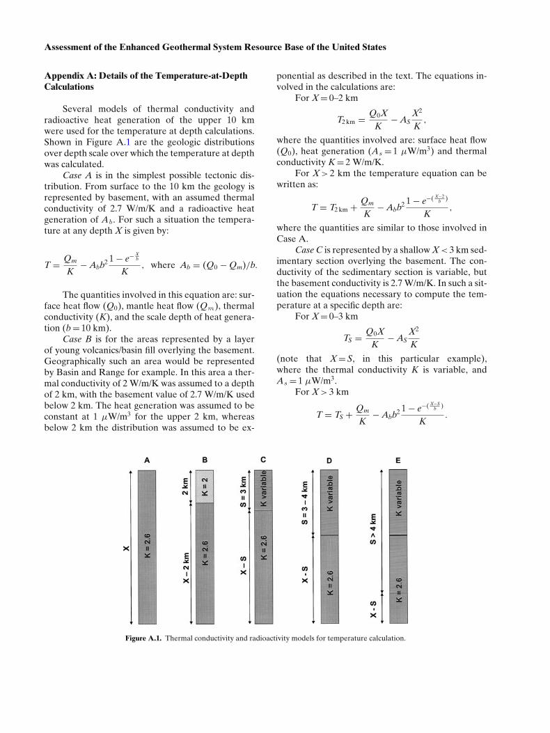
Assessment of the Enhanced Geothermal System Resource Base of the United States

Appendix A: Details of the Temperature-at-DepthCalculations

Several models of thermal conductivity andradioactive heat generation of the upper 10 kmwere used for the temperature at depth calculations.Shown in Figure A.1 are the geologic distributionsover depth scale over which the temperature at depthwas calculated.

Case A is in the simplest possible tectonic dis-tribution. From surface to the 10 km the geology isrepresented by basement, with an assumed thermalconductivity of 2.7 W/m/K and a radioactive heatgeneration of Ab . For such a situation the tempera-ture at any depth X is given by:

T = Qm

K− Abb2 1 − e− X

b

K, where Ab = (Q0 − Qm)/b.

The quantities involved in this equation are: sur-face heat flow (Q0), mantle heat flow (Qm), thermalconductivity (K), and the scale depth of heat genera-tion (b = 10 km).

Case B is for the areas represented by a layerof young volcanics/basin fill overlying the basement.Geographically such an area would be representedby Basin and Range for example. In this area a ther-mal conductivity of 2 W/m/K was assumed to a depthof 2 km, with the basement value of 2.7 W/m/K usedbelow 2 km. The heat generation was assumed to beconstant at 1 µW/m3 for the upper 2 km, whereasbelow 2 km the distribution was assumed to be ex-

ponential as described in the text. The equations in-volved in the calculations are:

For X = 0–2 km

T2 km = Q0XK

− ASX2

K,

where the quantities involved are: surface heat flow(Q0), heat generation (As = 1 µW/m3) and thermalconductivity K = 2 W/m/K.

For X > 2 km the temperature equation can bewritten as:

T = T2 km + Qm

K− Abb2 1 − e−( X−2

b )

K,

where the quantities are similar to those involved inCase A.

Case C is represented by a shallow X < 3 km sed-imentary section overlying the basement. The con-ductivity of the sedimentary section is variable, butthe basement conductivity is 2.7 W/m/K. In such a sit-uation the equations necessary to compute the tem-perature at a specific depth are:

For X = 0–3 km

TS = Q0XK

− ASX2

K

(note that X = S, in this particular example),where the thermal conductivity K is variable, andAs = 1 µW/m3.

For X > 3 km

T = TS + Qm

K− Abb2 1 − e−( X−S

b )

K.

Figure A.1. Thermal conductivity and radioactivity models for temperature calculation.

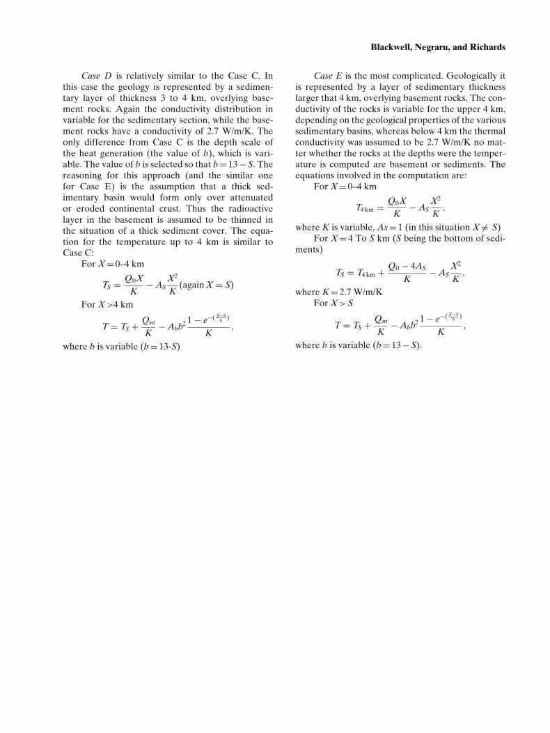
Blackwell, Negraru, and Richards

Case D is relatively similar to the Case C. Inthis case the geology is represented by a sedimen-tary layer of thickness 3 to 4 km, overlying base-ment rocks. Again the conductivity distribution invariable for the sedimentary section, while the base-ment rocks have a conductivity of 2.7 W/m/K. Theonly difference from Case C is the depth scale ofthe heat generation (the value of b), which is vari-able. The value of b is selected so that b = 13 − S. Thereasoning for this approach (and the similar onefor Case E) is the assumption that a thick sed-imentary basin would form only over attenuatedor eroded continental crust. Thus the radioactivelayer in the basement is assumed to be thinned inthe situation of a thick sediment cover. The equa-tion for the temperature up to 4 km is similar toCase C:

For X = 0–4 km

TS = Q0XK

− ASX2

K(again X = S)

For X >4 km

T = TS + Qm

K− Abb2 1 − e−( X−S

b )

K,

where b is variable (b = 13-S)

Case E is the most complicated. Geologically itis represented by a layer of sedimentary thicknesslarger that 4 km, overlying basement rocks. The con-ductivity of the rocks is variable for the upper 4 km,depending on the geological properties of the varioussedimentary basins, whereas below 4 km the thermalconductivity was assumed to be 2.7 W/m/K no mat-ter whether the rocks at the depths were the temper-ature is computed are basement or sediments. Theequations involved in the computation are:

For X = 0–4 km

T4 km = Q0XK

− ASX2

K,

where K is variable, As = 1 (in this situation X �= S)For X = 4 To S km (S being the bottom of sedi-

ments)

TS = T4 km + Q0 − 4AS

K− AS

X2

K,

where K = 2.7 W/m/KFor X > S

T = TS + Qm

K− Abb2 1 − e−( X−S

b )

K,

where b is variable (b = 13 − S).