assessment of shape changes of mistletoe berries: a new

Assessment of Shape Changes of Mistletoe Berries: ANew Software Approach to Automatize theParameterization of Path Curve Shaped ContoursRenatus Derbidge1,2*, Linus Feiten3, Oliver Conradt4, Peter Heusser1, Stephan Baumgartner1,5

1 Centre for Integrative Medicine, University of Witten/Herdecke, Witten, Germany, 2 Research Institute at the Goetheanum, Science Section, Dornach, Switzerland,

3 Faculty of Engineering, Chair of Computer Architecture, University of Freiburg, Freiburg, Germany, 4 Section for Mathematics and Astronomy, Goetheanum, Dornach,

Switzerland, 5 Hiscia Institute, Society for Cancer Research, Arlesheim, Switzerland

Abstract

Photographs of mistletoe (Viscum album L.) berries taken by a permanently fixed camera during their development inautumn were subjected to an outline shape analysis by fitting path curves using a mathematical algorithm from projectivegeometry. During growth and maturation processes the shape of mistletoe berries can be described by a set of such pathcurves, making it possible to extract changes of shape using one parameter called Lambda. Lambda describes the outlineshape of a path curve. Here we present methods and software to capture and measure these changes of form over time.The present paper describes the software used to automatize a number of tasks including contour recognition, optimizationof fitting the contour via hill-climbing, derivation of the path curves, computation of Lambda and blinding the pictures forthe operator. The validity of the program is demonstrated by results from three independent measurements showingcircadian rhythm in mistletoe berries. The program is available as open source and will be applied in a project to analyze thechronobiology of shape in mistletoe berries and the buds of their host trees.

Citation: Derbidge R, Feiten L, Conradt O, Heusser P, Baumgartner S (2013) Assessment of Shape Changes of Mistletoe Berries: A New Software Approach toAutomatize the Parameterization of Path Curve Shaped Contours. PLoS ONE 8(4): e60522. doi:10.1371/journal.pone.0060522

Editor: Rongling Wu, Pennsylvania State University, United States of America

Received September 26, 2012; Accepted February 28, 2013; Published April 2, 2013

Copyright: � 2013 Derbidge et al. This is an open-access article distributed under the terms of the Creative Commons Attribution License, which permitsunrestricted use, distribution, and reproduction in any medium, provided the original author and source are credited.

Funding: This paper is part of a research project funded by the "Software AG Stiftung", Darmstadt, Germany (http://www.software-ag-stiftung.com/) and the"Hiscia Institute", Society for Cancer Research, Arlesheim, Switzerland (http://www.vfk.ch/hiscia/). The funders had no role in study design, data collection andanalysis, decision to publish, or preparation of the manuscript.

Competing Interests: The authors have declared that no competing interests exist.

* E-mail: [email protected]

Introduction

Patterns and forms in animals and plants have fascinated

mankind from the dawn of science in ancient Greece, and

motivated thinkers and scientists at the beginning of the scientific

revolution. Patterns and forms seemed ideal for exploring the

hidden plan of God in nature [1], with mathematics the tool of

choice for revealing these ‘‘divine thoughts’’. Even today, in fact,

amazing correlations continue to be found between forms and

patterns in nature and certain fields in mathematics [2], and

modeling has developed into a viable instrument for revealing the

lawfulness of biological processes.

In chronobiology, mathematics and biology interact in a

peculiar way. Rhythms of plant growth and development, the

synchronicity of cell division and DNA replication are scrutinized,

as are gene expression and enzymatic activity in correlation with

time or season. Biological rhythms can also be found phenotyp-

ically in plant organs such as buds or berries [3].

Lawrence Edwards, a Scottish mathematician, discovered that

two-dimensional projections of a certain subgroup of path curves

[4,5,6], which are three-dimensional transformations of measures

in projective geometry [4,5,6,7], fit perfectly to the outline shape of

various plant buds [8]. Other researchers observed that the profile

of certain berries (e.g. of mistletoe, Viscum album L.) likewise accord

with path curves [9,10,11]. Edwards observed that the shape of

buds of various trees during dormancy in winter exhibited a

fortnightly rhythmic change of form [8]. One of many path curve-

defining parameters called Lambda (l) is needed to determine the

change of shape. l is of interest, since it defines the outline shape

of a path curve. Lambda allows the detection of possible

alterations of shape in time.

We aimed to investigate the reproducibility of Edwards’s results,

and to extend his approach to shorter timescales. This requires the

assessment of a large number of plant photographs, taken at short

intervals over a period of several weeks or even months. Form

analysis of buds or berries on the basis of such pictures evidently

requires software to automatize the process. Such software must

facilitate determination of the two-dimensional outline shape of

buds or berries.

The outline shape of a three-dimensional path curve, which is

defined by the parameter l can be deduced from the contour line

of the object captured in the photograph. The software recognizes

the outline as a contour line and extracts l by calculating the path

curve that best fits and corresponds to the outline shape of the

object.

Since some of the procedures require an operator’s deliberate

actions, the pictures must be analyzed in a random order and

without any knowledge of the time and day they were taken. To

our knowledge, appropriate software capable of performing these

tasks does not exist. Thus, we decided to design and implement a

program according to the specifications outlined above.

PLOS ONE | www.plosone.org 1 April 2013 | Volume 8 | Issue 4 | e60522

Results

The software developed is called ‘‘LambdaFit’’ and is currently

available as version 1.7. The program is freely available as open

source at http://www.feiten.de/LambdaFit/. Its main features are

described in the following paragraphs.

Import, randomization and coding of the imagesThe human operator of the software must not know which

picture he is currently evaluating. Otherwise he might subcon-

sciously bias the measurements. Therefore, the first task of

LambdaFit is to code a set of images.

The software prompts the operator to select a directory of

images, which are subsequently sorted in random order and listed

for the operator with coded numbers only (see Figure 1). In the

same directory, a file is created which stores this random order.

Should a new order be needed, it suffices to delete the first file.

The operator looking at the interface of the software only sees

the number of measurements performed for a given set of images.

Thus, it is possible to repeat measurements for one and the same

folder in different random orders, and without the risk of

inadvertently missing a picture (see Figure 1).

The software’s graphic user interface has some features to make

use as convenient as possible. After opening a folder of

photographs (JPEGs) the feature ‘‘,’’ and ‘‘.’’ lets the operator

skip from file to file, shown in the bottom text box. The ‘‘Jump to

file’’ text box can be used to directly select a specific file. ‘‘Take

new measurement’’ opens the windows to determine the best path

curve parameters. The optimization process can then begin (see

below). Further features give the opportunity to change some

parameters of the path curve, which are pre-set as shown in the

interface box. The text fields ‘‘Threshold’’ define the value for

contour recognition. This is the value indicating the lightness or

darkness of the threshold to decide if a pixel will be defined as

black or white. The box ‘‘Lambda*1000’’ can be used to define the

start value of l, as buds and berries, for instance, have a quite

different l-value. Definition of those two parameters will be saved

for the ‘‘Take new measurement’’ part, and stay the same until

changed again.

Recognition of the plant contourIn order to compute the parameters of the path curve with best

fit to the biological sample, the software must first facilitate shape

identification. Free graphics library openCV [http://opencv.

willowgarage.com/] is very well suited for this task, since it

already provides many computer vision functionalities, such as

recognition of contours in images [12].

In order to detect contours in a picture, the latter first has to be

converted into a binary image composed exclusively of black and

white pixels. The threshold level must be set by a human operator,

based on the picture’s lighting. Figure 2 shows different outcomes

for different threshold values.

It is very important that the outline of the photographed object

is clearly silhouetted against the background and not blurred.

Varying thresholds lead to different shapes determined by

LambdaFit. Based on the binary image (middle) in Figure 2, the

software is able to derive the sample’s contour as depicted in

Figure 3.

Drawing the path curveThe software calculates and draws a complete path curve,

whose starting position, shape and orientation can be adjusted by

changing a set of parameters (see below). In a second step, the

parameter values can be deduced for the best fitting path curve,

i.e. that of maximum congruency. Details of the algorithm used

and the optimization process are described in the section ‘‘Design

and Implementation’’. Figure 4 shows the appearance of a picture

at the stage of measurement as described above. The drawn path

curve is visible for the user as a red line according with the

different parameters that define the shape and the position of the

path curve outline (see Figure 5).

Extraction of LambdaLambda (l) is one of the shape-defining parameters in a three-

dimensional path curve. It determines the outline, i.e. the two-

dimensional contour of a path curve. The numerical value ‘‘1’’ is

an equilibrium between the two variations of ‘‘egg-shapes’’,

Figure 1. Graphic user interface. In this case the original files fromthe folder ‘‘plant_samples’’ are shown in random order. Files 2 and 5have been measured once, file 4 has been measured twice, and theother files shown have not been measured yet. File 3 is selected. Thevalues of the fitted parameters are saved automatically in a file notvisible in this interface in the same folder as a ‘‘csv’’-file.doi:10.1371/journal.pone.0060522.g001

Figure 2. Drawing the contour (threshold function). Original photograph of a mistletoe berry (left) with two binary conversions: with adequatethreshold (center), with inadequate threshold (right).doi:10.1371/journal.pone.0060522.g002

Assessment of Shape Changes of Mistletoe Berries


meaning it has the same acumination or flatness on both of its

ends. For l $ 1 the top is sharper and the bottom flatter. For 0 ,

l #1 the path curve will be the opposite, sharp at the bottom and

flat at its top (see Figure 6). l describes the relation between the

shape of the path curve’s top and bottom. l is not an absolute

value describing a certain shape: the l-value can stay the same

while height or width of the path curve changes. For l , 0 the

path curves transform into vortex-like forms. Figure 6 gives an

impression of different l-values as present in mistletoe berries.

LambdaFit produces a path curve arising from preset param-

eters such as width, height and l. These values can also be

manipulated manually (see Figure 5). If not manually set, the

software uses the preset values as determined in the opening

window (as shown in Figure 1). The position of the drawn path

curve within the photograph can be changed by rotation and

translation on the x- and y- axis. Again, the software draws the

position of the path curve according to the modified values.

In order to obtain an optimal fit, it is necessary to place the

starting path curve at a reasonable position. This step is critical.

The operator has to define the line of symmetry or mirror axis, i.e.the top and bottom of the path curve. The operator has the

possibility of defining this position via a number of ‘‘hot-keys’’ in

combination with the cursor (computer mouse), for example, by

pressing the hot-key ‘‘M’’ to define the mirror axis. ‘‘M’’ has to be

pressed, then the cursor must be moved to the corresponding

points: top first, and clicking, sets the position; then bottom, and

clicking again, sets the axis point at the base of the object within

the photograph (see Figure 7 middle). This choice of an adapted

starting position will make the path curve fitting process

considerably faster, since the overlapping of the contour (yellow

line) and the path curve (red line) is already quite good. Figure 7

(right) shows an optimized path curve. The hot-keys ‘‘P’’ and ‘‘O’’

are available to start the curve fitting process. ‘‘P’’ optimizes the

path curve by finding the best congruency with all parameters (see

details in Design and Implementation), and ‘‘O’’ starts an

optimization process that mainly considers the width of the path

curve.

An additional window facilitates the optical differentiation of the

congruency between the real berry’s outline shape (the yellow line)

and the mathematical path curve, respectively the l-line (red).

This is a helpful tool, since overlapping is often so close that it is

impossible to judge by eye whether further optimization is possible

(as shown in figure 7 right). The ‘‘deviation’’ window transfers the

Figure 3. Contour line. The contour of the mistletoe berry in Fig. 2, asdetermined by LambdaFit.doi:10.1371/journal.pone.0060522.g003

Figure 4. Contour and calculation line for the path curve.Composite picture of a mistletoe berry with the contour in yellow andthe calculated – not yet fitted – path curve in red.doi:10.1371/journal.pone.0060522.g004

Figure 5. ‘‘Trackbar’’ window. All necessary parameters are shownin an additional window that contains slides for manual adaptation ofthe parameters of the path curve to the contour.doi:10.1371/journal.pone.0060522.g005



two curved lines from the output window into straight lines and

automatically translates the scale to a maximum difference

between them. This presents the user with more information

instead of only the average, stored distance. The distance between

the lines is shown in pixel units starting from the top (center in

figure 8) to bottom (far ends on both sides in figure 8) of the object

i.e. berry. This enables the user to alter the variables by hand via

the sliders (see figure 5) because the optimization algorithm is

searching for a global minimum and often ‘‘ignores’’ local

noticeable problems, which the deviation window makes visible

(see ‘‘Fitting the path curve’’ in the ‘‘Design and Implementation’’

section). Figure 8 demonstrates the situation of an unequally fitted

path curve. On the far left side (meaning, near the bottom of the

berry’s left side) the congruency is not as good as may be possible

(there is 3.6 pixels difference between the mathematical path curve

and the biological shape instead of 1 pixel distance, as this is the

difference in most of the other regions of the berry’s outline

(dominant yellow straight line in figure 8)).

Storing the resultsResults (i.e. path curve parameters, energy function value and

the time the measurement was performed) are stored in a result

file. Accompanying data in this file are the real names of the

images of each measurement and the time the image was taken.

The latter is automatically extracted from the JPEG exif data.

The file saving the measurements is a comma-separated value

file (csv) and can be opened and processed by any statistical or

spreadsheet application.

Internal validityThe quality of the extracted data is sensitive to the operator’s

intervention at two points: the identification of the contour, and

the fitting of the path curve, respectively. Thus, the necessary and

sufficient number of replicate measurements per image had to be

determined. Three independent evaluation runs were performed

on a set of 144 pictures. They were obtained from a single berry on

a mistletoe bush (Viscum album ssp. album) growing on oak (Quercus

robur), located in Arlesheim, Switzerland. The berry was photo-

graphed from a fixed distance and angle every hour for six days in

October 2011. Former observations led us to expect a circadian

rhythm in the changes to the berry’s shape (see Figure 9).

Two questions had to be answered: first, is it possible to

reproduce one’s own measurements? For this setting the same

person repeated the identical set again after a longer period of time

(P1 and P2 is the same person). The second question was: is it

possible for a different operator to achieve the same results? In this

setting a different person P3 did the computation. All photos were

measured in random order as described above. To minimize

random error, each photo was measured repeatedly. P1 and P3

had 10 repeats per photo; P2 had 6 repeats per photo.

Figure 9 displays the mean l value of all repeats per photo.

Additionally, a weighted fit has been added because it reveals the

signal within the data, making the rhythmic change of l visible at

first sight. The software KaleidaGraph 4.0 (Synergy Software,

Reading PA) was used to draw a weighted fit using LOWESS,

locally weighted regression scatter plot smoothing [13]. For each

data point this operation defines a linear regression equation, in

which a certain percentage P of the neighboring weighted data

points is included. The function thus calculates a smoothed curve;

the larger the percentage P of included neighboring data points,

the smoother the curve.

In Figure 9 an approximately circadian rhythm could be

identified for P1, P2 and P3. The l data were thus compiled on a

24 h scale to compare the measurements in more detail. First, the

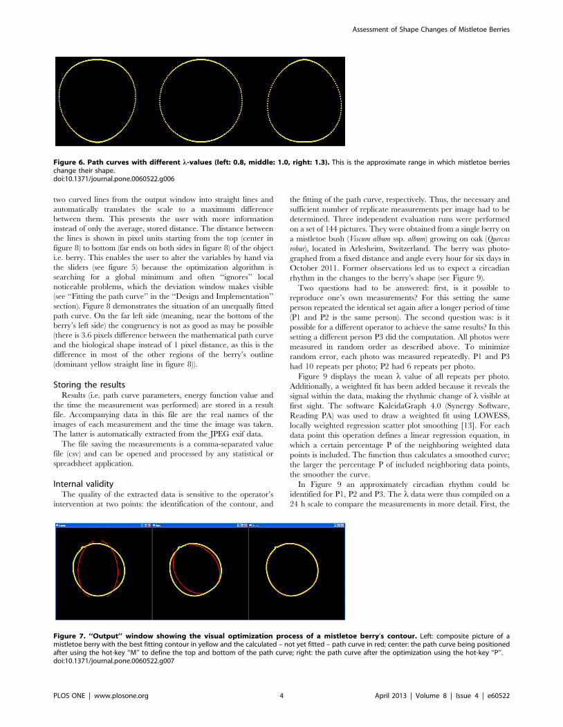
Figure 6. Path curves with different l-values (left: 0.8, middle: 1.0, right: 1.3). This is the approximate range in which mistletoe berrieschange their shape.doi:10.1371/journal.pone.0060522.g006

Figure 7. ‘‘Output’’ window showing the visual optimization process of a mistletoe berry’s contour. Left: composite picture of amistletoe berry with the best fitting contour in yellow and the calculated – not yet fitted – path curve in red; center: the path curve being positionedafter using the hot-key ‘‘M’’ to define the top and bottom of the path curve; right: the path curve after the optimization using the hot-key ‘‘P’’.doi:10.1371/journal.pone.0060522.g007



l values were normalized per day (mean set to 100%). Second,

mean values were calculated for each hour of the day, based on

the data obtained on the six days. These values were plotted

together with standard errors (Figure 10).

A LOWESS fit (P = 30%) reveals a comparable signal within the

data: l exhibits a circadian rhythm of<0.5%. It is above the

average between 0.00–12.00 am, and below average from noon to

midnight. Minima and maxima vary to some extent between

operators and repetition of the measurements.

Daily change data of the three measurement series, the hourly

mean values (blue points in Figure 10) as well as the data of the

weighted fit in hourly resolution (violet lines in Figure 10), were

correlated (see Table 1) between P1, P2 and P3. For the

correlation analysis we used the Pearson product moment

correlation test with Statistica 6.0 (StatSoft, Tulsa, USA).

Comparison of the hourly mean values of P1 with those of P2

yields a highly significant correlation coefficient (p , 0.0001, n =

24). The same applies to the data of the weighted fit (p , 0.0001,

n = 24).

The correlation analysis for P2 and P3 gives a value of the

correlation coefficient of r = 0.60 (p = 0.0019, n = 24), which is

less pronounced than the correlation between P1 and P3 (r =

0.79). The reason for this is most probably of technical nature,

since the data for the circadian rhythm of P2 were compiled from

six repeated Lambda determinations (instead of 10 for P1 and P3).

For the future, means of 10 repeated Lambda determinations per

photograph will be used.

The significant correlations show that both the handling of the

data and the high-level functionality of the software developed will

allow robust operation.

Design and Implementation

Drawing the path curveThe function used in drawing a 2-dimensional path curve

contour is:

f : IR?IR|½0,h� [ IR|IR

f (t)~1

e{ltz h2

et: +w,

eth2

2

� �

This function can be derived by using the continuous

transformation matrix

Pt~

exp (vt) 0 0

0 1 0

0 0 exp ({svt)

0B@

1CA

for a plane path curve with three real and different eigenvalues

with v = 1 and s = l [14, p. 20].

On the other side it is possible to derive the path curve funktion

f starting from the equations (14) and (15) from Almon [6]:

Figure 8. ‘‘Deviation’’ window. The distance in pixels is shown forevery point (in pixels) along the path curves lambda line (red) to theberries outline shape (yellow). In this case the congruency is quite high.In almost all the events the distance is ‘‘0’’ or ‘‘1’’ pixel difference;toward the bottom of the berry (both ends of the lines), congruencydeteriorates however to a maximum of 3.6 pixels distance on the leftside.doi:10.1371/journal.pone.0060522.g008

Figure 9. Three independent measurements of Lambda (P1, P2, P3), based on 144 pictures of the same mistletoe berry (24 picturesper day in the course of six days). P1 (red dots) and P2 (blue circles) are two independent measures by the same person, P3 (green circles) by adifferent person. Every data point represents the mean of several measurements (n = 10 for P1 and P3, n = 6 for P2). Error bars were omitted for clarity.The smooth continuous lines represent LOWESS fits with P = 10% (red: P1, blue: P2, green: P3).doi:10.1371/journal.pone.0060522.g009



p3(t)~c exp (t)

c exp (t)z1

r(t)~B exp (vt)

c exp (t)z1

Almon is using as independent variable t for p3(t) and t = t for

r(t). In order to be unambigous, we continue to use t as

independent variable, which corresponds to equation (15) of

Almon.

Substituting t, c, B and v according to

t~(1zl)t

c~h

2

B~v

v~l

lz1

one gets the path curve equation needed for the software:

(+r(t),h:p3(t))~1

e{ltzh

2et

: +w,eth2

2

� �

~f (t)

The 6 sign in the x-coordinate indicates that f draws the right

and the left side of the path curve simultaneously. Multiplication of

p3(t) with h in the y-coordinate is needed to get an arbitrary

height.The limit values for the domain IR are f (–‘) = (0,0) and f

(‘) = (0,h):

limt?{?

f (t)

~ limt?{?

1

e{ltzh

2et

: +w,eth2

2

� �

~ limt?{?

+w

e{ltzh

2et

,eth2

2e{ltzhet

0B@

1CA

~ +w

?z0,

0

?z0

� �

~ +0,0ð Þ

limt??

f (t)

~ limt??

1

e{ltzh

2et

: +w,eth2

2

� �

~ limt??

+w

e{ltzh

2et

,eth2

2e{ltzhet

0B@

1CA

~ +w

0z?,

limt??

eth2

0z limt??

eth

0@

1A

~ +0, limt??

eth2

eth

� �

~ +0, limt??

h2

h

� �

~ +0,hð Þ

Thus, h can be considered the parameter defining the path

curve’s height. The other two constants in f are w and l. w can be

considered the parameter defining the path curve’s width, as it is

simply a factor for the curve’s y-coordinates. The most interesting

Figure 10. Daily change of Lambda of a mistletoe berry (mean ± SE) for three independent measurements (P1, P2, P3). Data from Fig.9 were normalized for each day and averaged. P1 and P2 are two independent measures by the same person, P3 are measurements by a differentperson. The smooth continuous lines are LOWESS fits (P = 30%).doi:10.1371/journal.pone.0060522.g010



parameter is l, which defines the characteristic form of the curve;

pointed top, round or pointed bottom (see Figure 6).

The task for our software is to find the parameters h, w and l, so

that the resulting path curve has an optimal congruence with the

measured plant contour from the picture. The measured contour

can, however, be located and oriented anywhere in the

photograph. So we also need rotation, horizontal and vertical

translation as parameters a, x and y. Adding these to f, we get:

g : IR?IR|IR

g(t)~1

e{ltzh

2et

:+w: cos a{

eth2

2: sin azx

+w: sin a{eth2

2: cos azy

0BBB@

1CCCA

T

With this set of six parameters the program is able to draw every

possible path curve, showing always only the two-dimensional l-

shape. In the next step, we have to decide how many points of g

we want to calculate. As the domain of t is IR, the path curve

consists of an infinite number of points. For equidistant t values

however, the resulting points g(t) are found to lie more densely

toward the top and bottom of the path curve (Fig. 11).

It is therefore sufficient to calculate values from t = 220 to

t = 20. To obtain enough intermediate points we chose a step size

of 0.05 between the different t values, which led to a total of 801

calculated points for each side (left and right) of the path curve.

As shown in figure 11, the calculated points are connected with

straight red lines. Thus, we can get all pixel coordinates of the

calculated path curve, including the points between the ones

calculated by g(t). If the step size between subsequent values of t is

sufficiently small – which is the case for 0.05 – the gaps between

the calculated points are so small that the path curve seems to

exhibit a round shape, even if single points are connected by

straight lines. Thus the calculated path curve has no continuous

curvature. This deviation from an ideal path curve is negligible,

however, compared with the photographs’ resolution, and

naturally occurring variations in biological shape.

Fitting the path curveThe software has to bring the pixels of the measured plant

contour and the pixels of the calculated path curve into

congruence by finding the optimal parameters l, h, w, a, x and

y. This is achieved by a so-called hill-climbing algorithm. We start

with an arbitrary path curve and check how congruent it is with

the plant contour. Then we change its parameters and check

again. If the new parameters yield a more congruent path curve

we keep the new ones, and repeat the procedure. Eventually the

best fitting path curve is found. We will discuss the details of this

algorithm below. Before this, we describe how the software checks

the degree of congruence of a calculated path curve with the

measured plant contour.

Congruency of the two curves is estimated by a so-called energy

function, as input of the two contours. A lower value is returned if

these are more congruent, and a higher value if they are less

congruent. To achieve this, we perform a distance transformation

on the image of the measured plant contour.

The distance transformation can be done by another method of

openCV [15]. After the distance transformation of a plant contour

image (see figure 2 for an example), the newly generated image

contains for each pixel the Euclidian distance of this pixel from the

nearest plant contour pixel (see Figure 12).

By means of this distance transformation we can immediately

determine the distance of each pixel in the calculated path curve

from the measured plant contour by checking the values of each

pixel in the distance transformation image with the coordinates of

the pixels in the path curve. The greater the distance between the

calculated path curve and the plant contour, the higher is the sum

of all these values. Thus it makes sense to define this sum as energy

function. The perfectly fitted path curve would produce an energy

function value of 0, because every pixel lies on the measured plant

contour.

Letting n be the number of all pixels in the calculated path

curve, and letting disti be the value of the coordinates belonging to

pixel i in the distance transformation image, our energy function

could be defined as:

e~

ffiffiffiffiffiffiffiffiffiffiffiffiffiffiffiffiPnt~1

distt

n

vuuut

To allow statistical interpretation, we modified this energy

function by summing the squares of the distances, and thus

essentially arrived at the usual least-squares fitting procedure:

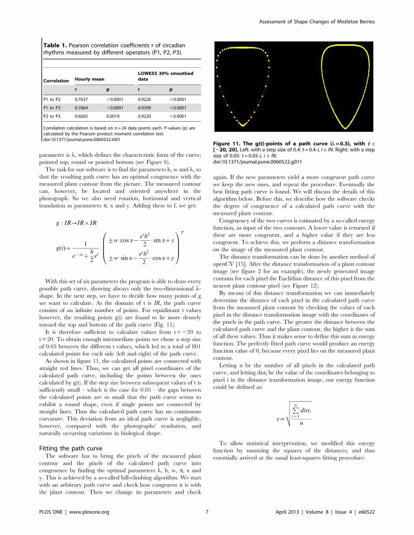
Table 1. Pearson correlation coefficients r of circadianrhythms measured by different operators (P1, P2, P3).

Correlation Hourly meanLOWESS 30% smootheddata

r p r p

P1 to P2 0.7637 ,0.0001 0.9226 ,0.0001

P1 to P3 0.7864 ,0.0001 0.9399 ,0.0001

P2 to P3 0.6005 0.0019 0.9220 ,0.0001

Correlation calculation is based on n = 24 data points each. P-values (p) arecalculated by the Pearson product moment correlation test.doi:10.1371/journal.pone.0060522.t001

Figure 11. The g(t)-points of a path curve (l = 0.3), with t M[220, 20]. Left: with a step size of 0.4: t = 0.4?i, i M IN. Right: with a stepsize of 0.05: t = 0.05?i, i M IN.doi:10.1371/journal.pone.0060522.g011



e~

ffiffiffiffiffiffiffiffiffiffiffiffiffiffiffiffiffiPnt~1

dist2t

n

vuuut

With the energy function defined as above, we can come back to

the hill-climbing algorithm. As mentioned above, the algorithm

can start with an arbitrary path curve. It then alters some (or all) of

the six parameters of g(t), which define the path curve, by a certain

proportion d and checks if these changes yield a path curve more

congruent with the plant contour. If so, the new parameter values

are kept and the procedure starts again. If no better path curve can

be found, the algorithm does not stop but decreases d. Thus, the

longer the search lasts, the more fine-tuned it becomes. If dreaches a certain minimal value, the algorithm stops and a

minimum of the energy function is found. The following pseudo

code illustrates this:

curve: = initial_curve;

d: = 0.5;

while (d .0.005) {

found_better: = true;

while (found_better) {

found_better: = false;

‘‘Alter the parameters of curve by d

(several alterations are possible)’’

if (alteration_k is better than curve) {

curve: = alteration_k;

found_better: = true;

}

}

d: = d/1.6;

}

Of course, this hill-climbing algorithm is prone to not finding

the global minimum, but only a local minimum of the energy

function. To overcome this, the human software operator has to

supervise the algorithm by means of a graphic user interface,

which shows the original plant image, the recognized plant

contour and the calculated path curve in one image (see Figure 4).

Streamlining the optimization processIn Figure 4 it can be seen that the top and bottom of the

calculated path curve are excluded. This ‘‘cut off’’ functionality

was integrated because of the actual habitus of the plant. The

bottom parts of mistletoe berries deviate from ideal path curves

due to their fixation at the stipe (peduncle). Correspondingly, the

berry-shape is not always clearly identifiable by the software.

Likewise, the little cap on top of the berries does not belong to the

path curve shape of the berry. In order not to let these

irregularities have an impact on the energy function, we can set

top and bottom of the path curves for exclusion from the

measurement.

Another peculiarity of mistletoe berries is that they are almost

round. This makes it almost impossible for the hill-climbing

algorithm to find the correct rotation of the path curve. We

therefore enabled the human operator to define the coordinates of

the top and bottom of the path curve by clicking at the positions in

the image. The algorithm then runs in a mode where no greater

variations of the rotation are allowed, because the orientation set

by the operator is maintained.

We also found that the hill-climbing algorithm works particu-

larly well if we first let it optimize only the width parameter w of

the path curve, followed by an optimization cycle for the lparameter only, followed by a last cycle in which again variations

of all six parameters were allowed.

To enhance the optimization we also applied slight changes to

the path curve-drawing function g(t),. One change was that an

alteration of a would lead to a rotation of the path curve around its

center, instead of around its top, which was the case for the

original g(t) function. Another change was that we always multiply

the current parameter value of w with the current value of l, and

use this product for w. This compensates for the overall effect

which an alteration of l has on the path curve’s width. With this

change, an alteration of l mainly affects the bow of the curve

rather than its width.

Conclusion and Future Work

The program may be improved by future users so as to offer

more pre-set versions of the variable values at the starting process

when importing a file, to accommodate the precise indicator of

phenotypical change of shape in berries or buds. A circadian

rhythm in mistletoe berries has been found and will be investigated

further. Different, long-frequency rhythms will be studied as well.

The software will be applied to study of the leaf buds of mistletoe

host trees, in order to search for interactions in rhythm.

Corresponding rhythms or rhythmical interactions of mistletoe

berries and the leaf buds of mistletoe host trees will give valuable

insights into the biology of parasitism, i.e. mutualism in plant

biology.

Availability and future directionsThe software called LambdaFit is available along with further

directions and bud and mistletoe berry samples at http://www.

feiten.de/LambdaFit. We are also offering its source code for free

download and further development together with compilation

Figure 12. Plant contour from Fig. 3 after distance transfor-mation. Each pixel coordinate holds as its value the Euclidean distancebetween the pixel itself and the closest pixel of the plant contour. Thedarker a pixel, the closer it is to the plant contour.doi:10.1371/journal.pone.0060522.g012



instructions. More information on the libraries used, and their

availability, are included on the website as well.

Acknowledgments

Many thanks to Olaf Ronneberger for providing indispensable advice

concerning the software’s optimization algorithm. Also the authors would

like to thank Joan Davis, Johannes Wirz and Ernst Zurcher for helpful

comments on the manuscript.

Author Contributions

Conceived and designed the experiments: RD LF PH SB. Performed the

experiments: RD LF PH SB. Analyzed the data: RD SB. Contributed

reagents/materials/analysis tools: RD LF OC PH SB. Wrote the paper:

RD LF OC. Designed the software: LF. Optimized the software: RD.

Evaluated the software: RD LF SB. Statistics: RD SB PH.

References

1. Arber A (1950) Natural Philosophy of Plant Form. Cambridge: University Press.

246 p.

2. Kappraff J (2002) Beyond Measure: A Guided Tour Through Nature, Myth,

and Number. New Jersey: World Scientific. 582 p.

3. Dunlap J, Loros J, DeCoursey P (2004) Chronobiology: Biological Timekeeping.

Sunderland: Sinauer Associates. 405 p.

4. Klein F (2006) Lectures on Non-Euclidean geometry [German original entitled:

Vorlesungen uber nicht-euklidische Geometrie]. Saarbrucken: Vdm Verlag M.

Muller 338 p.

5. Klein F (2006) Introduction to higher geometry … by F Klein. Elaborated by Fr.

Schilling [German original entitled: Einleitung in die hohere Geometrie … Von

F Klein. Ausgearb. Von Fr. Schilling]. Ann Arbor; Univ of Michigan Lib. 576 p.

6. Almon C (1994) Path Curves, an Introduction to the Work of L. Edwards on

Bud Forms. Open Sys. & Information Dyn. 2: 265-277.

7. Edwards L (2003) Projective Geometry. Edinburgh: Floris Books. 347 p.

8. Edwards L (2006) The Vortex of Life: Nature’s Patterns in Space and Time.

Edinburgh: Floris Books. 381 p.

9. Fluckiger H, Baumgartner S (2003) Shape changes of ripening mistletoe berries.

Archetype. 9: 1-13.

10. Baumgartner S, Fluckiger H, Ramm H (2004) Mistletoe berry shapes and the

zodiac. Archetype. 10: 1-20.11. Sonder G (1993) Mistletoe and host-tree forms as the foundation for mixing

processes [German original entitled: Mistel und Wirtsform als Grundlage zurGestaltung von Mischprozessen]. Elemente der Naturwissenschaft. 58: 37-63.

12. Find contours. Structural Analysis and Shape Descriptors. [Online]. Open CV

website. Available: http://opencv.willowgarage.com/documentation/structural_analysis_and_shape_descriptors.html?highlight = cvfindcontours#cvFindContours.

Accessed 2012, Jul 30.13. Chambers JM, Cleveland WS, Kleiner B, Tukey PA (1983) Smoothing by

Lowess. In: Chambers JM, Cleveland WS, Kleiner B, Tukey PA. Graphical

Methods for Data Analysis. Belmont: Wadsworth International Group. pp. 94–104

14. de Boer L (2004) Classification of real projective Pathcurves. Mathematisch-Physikalische Korrespondenz. 219: 4-48. Available: http://mas.goetheanum.

org/deboer.html.15. Dist Transform. Miscellaneous Image Transformations. [Online]. Open CV

website. Available: http://opencv.willowgarage.com/documentation/

miscellaneous_image_transformations.html?highlight = disttrans#cvDistTransform.Accessed 2012, Jul 30.



assessment of shape changes of mistletoe berries: a new

Documents