assessment of effective dose in computed tomography …homepage.eircom.net/~gabbo1/documents/thesis...

Assessment of Effective Dose in Computed Tomography using an Anthropomorphic

Phantom

Paul Collins, B.E.

Thesis for the degree of M.Sc. of the National University of Ireland, Galway

Submitted September 2005

Department of Experimental Physics National University of Ireland, Galway

Head of Department: Prof. Thomas J. Glynn

Course Director: Prof Wil van der Putten

Supervisor: Brendan Tuohy

This candidate confirms that the work submitted is his own and that appropriate credit has been made to the work of others

Dedication

For my parents

ii

Table of Contents

1 Background and Introduction..................................................................... 1 1.1 Introduction ............................................................................................... 1 1.2 Research Motivation .................................................................................. 1 1.3 Research Objectives................................................................................... 1 1.4 History of CT............................................................................................. 2 1.5 Multi-Slice Computed Tomography (MSCT) ............................................. 3

1.5.1 What is MSCT ................................................................................... 3 1.5.2 Benefits and Disadvantages of MSCT ................................................ 4 1.5.3 Why MSCT has increased patient dose? ............................................. 5

1.6 Standard Imaging Protocols ....................................................................... 8 1.6.1 How changes in scan protocols affect patient dose.............................. 8 1.6.2 Scan Parameters Overview................................................................. 9

1.7 Patient Dosimetry in CT........................................................................... 10 1.7.1 Introduction...................................................................................... 10 1.7.2 Radiation Quantities......................................................................... 10 1.7.3 Thermoluminescence Dosimetry ...................................................... 12 1.7.4 Patient dose measurement ................................................................ 13 1.7.5 Other Methods of Evaluating Patient Dose ....................................... 13

1.8 Guidelines on Quality Criteria for CT ...................................................... 16 1.9 Radiation Risks........................................................................................ 17 1.10 Summary ................................................................................................. 17

2 Experimental Methods and Materials ...................................................... 18

2.1 Introduction ............................................................................................. 18 2.2 Thermoluminescence Dosemeters Setup .................................................. 19

2.2.1 Introduction...................................................................................... 19 2.2.2 Handling of TLDs ............................................................................ 19 2.2.3 Irradiation ........................................................................................ 19 2.2.4 Annealing & Cooling ....................................................................... 21 2.2.5 TLD Readout ................................................................................... 21 2.2.6 Reader Calibration ........................................................................... 24 2.2.7 Field Dosimeters Calibration ............................................................ 26 2.2.8 Linearity of Field Dosimeters ........................................................... 27

2.3 Anthropomorphic phantom ...................................................................... 28 2.4 Organ Measurement................................................................................. 29

2.4.1 Introduction...................................................................................... 29 2.4.2 Organ Selection................................................................................ 30 2.4.3 Distribution of TLDs........................................................................ 31 2.4.4 Placement of TLDs .......................................................................... 32 2.4.5 Summary.......................................................................................... 38

2.5 CT Scanners and Protocols Examinations ................................................ 39 2.6 Summary ................................................................................................. 40

iii

3 Results and Discussions ............................................................................. 41

3.1 Introduction ............................................................................................. 41 3.2 TLD Analysis .......................................................................................... 43 3.3 Diagnostic Protocols ................................................................................ 44

3.3.1 Abdomen/Pelvis Protocol ................................................................. 44 3.3.2 Head Protocol .................................................................................. 48 3.3.3 Chest Protocol.................................................................................. 52 3.3.4 Comparison with recent studies and Dosimetry Guidelines............... 55

3.4 Radiotherapy Protocols ............................................................................ 57 3.5 Summary ................................................................................................. 59

4 CONCLUSIONS........................................................................................ 60

4.1 Diagnostic Protocols ................................................................................ 60 4.2 Radiotherapy Protocols ............................................................................ 61 4.3 Future Considerations .............................................................................. 62

Appendix I ............................................................................................................. 63 Appendix II............................................................................................................ 68 References.............................................................................................................. 83

iv

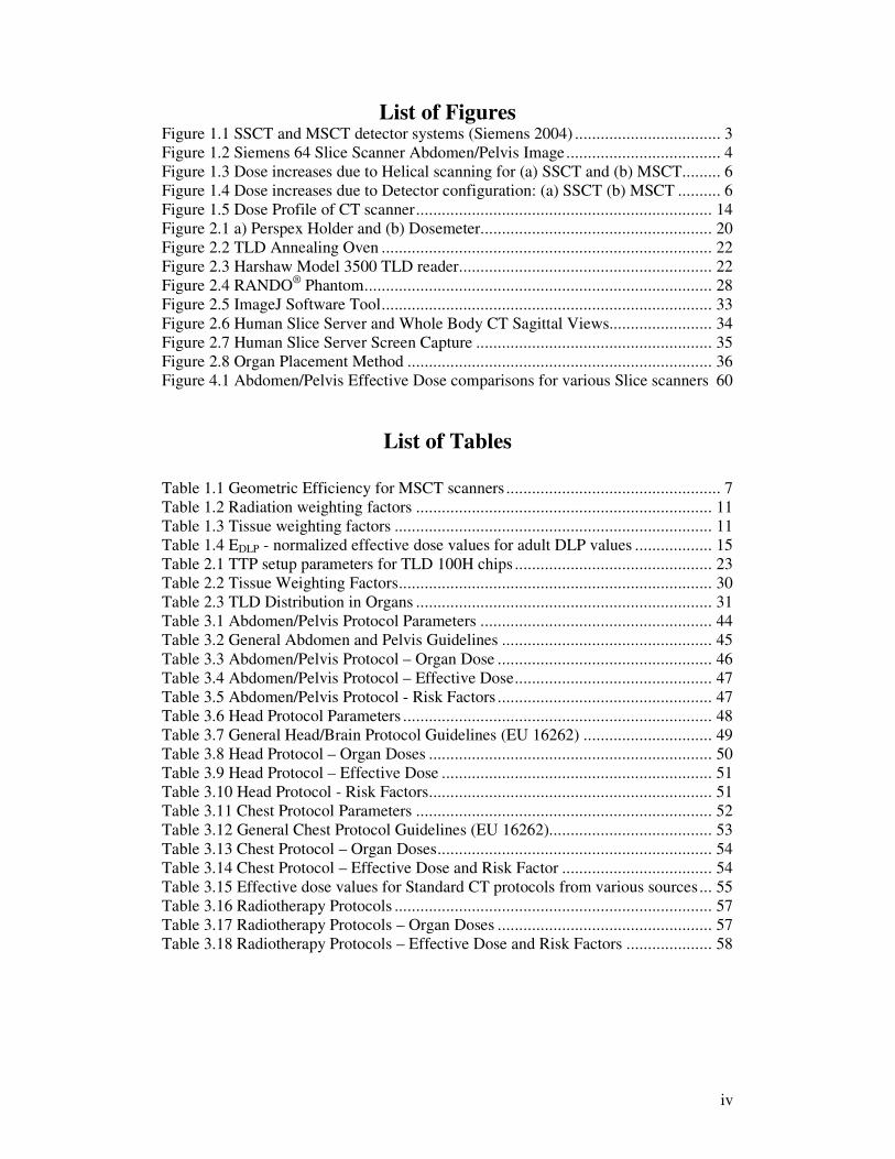
List of Figures Figure 1.1 SSCT and MSCT detector systems (Siemens 2004) .................................. 3 Figure 1.2 Siemens 64 Slice Scanner Abdomen/Pelvis Image.................................... 4 Figure 1.3 Dose increases due to Helical scanning for (a) SSCT and (b) MSCT......... 6 Figure 1.4 Dose increases due to Detector configuration: (a) SSCT (b) MSCT .......... 6 Figure 1.5 Dose Profile of CT scanner..................................................................... 14 Figure 2.1 a) Perspex Holder and (b) Dosemeter...................................................... 20 Figure 2.2 TLD Annealing Oven ............................................................................. 22 Figure 2.3 Harshaw Model 3500 TLD reader........................................................... 22 Figure 2.4 RANDO® Phantom................................................................................. 28 Figure 2.5 ImageJ Software Tool............................................................................. 33 Figure 2.6 Human Slice Server and Whole Body CT Sagittal Views........................ 34 Figure 2.7 Human Slice Server Screen Capture ....................................................... 35 Figure 2.8 Organ Placement Method ....................................................................... 36 Figure 4.1 Abdomen/Pelvis Effective Dose comparisons for various Slice scanners 60

List of Tables Table 1.1 Geometric Efficiency for MSCT scanners .................................................. 7 Table 1.2 Radiation weighting factors ..................................................................... 11 Table 1.3 Tissue weighting factors .......................................................................... 11 Table 1.4 EDLP - normalized effective dose values for adult DLP values .................. 15 Table 2.1 TTP setup parameters for TLD 100H chips .............................................. 23 Table 2.2 Tissue Weighting Factors......................................................................... 30 Table 2.3 TLD Distribution in Organs ..................................................................... 31 Table 3.1 Abdomen/Pelvis Protocol Parameters ...................................................... 44 Table 3.2 General Abdomen and Pelvis Guidelines ................................................. 45 Table 3.3 Abdomen/Pelvis Protocol – Organ Dose .................................................. 46 Table 3.4 Abdomen/Pelvis Protocol – Effective Dose.............................................. 47 Table 3.5 Abdomen/Pelvis Protocol - Risk Factors .................................................. 47 Table 3.6 Head Protocol Parameters ........................................................................ 48 Table 3.7 General Head/Brain Protocol Guidelines (EU 16262) .............................. 49 Table 3.8 Head Protocol – Organ Doses .................................................................. 50 Table 3.9 Head Protocol – Effective Dose ............................................................... 51 Table 3.10 Head Protocol - Risk Factors.................................................................. 51 Table 3.11 Chest Protocol Parameters ..................................................................... 52 Table 3.12 General Chest Protocol Guidelines (EU 16262)...................................... 53 Table 3.13 Chest Protocol – Organ Doses................................................................ 54 Table 3.14 Chest Protocol – Effective Dose and Risk Factor ................................... 54 Table 3.15 Effective dose values for Standard CT protocols from various sources... 55 Table 3.16 Radiotherapy Protocols .......................................................................... 57 Table 3.17 Radiotherapy Protocols – Organ Doses .................................................. 57 Table 3.18 Radiotherapy Protocols – Effective Dose and Risk Factors .................... 58

v

Abstract

Patient dose from CT examinations is increasing and this can be correlated with the

evolution of CT technology and the subsequent changes in clinical practice.

Conventional single slice CT (SSCT) has now been replaced with Multi-Slice CT

(MSCT). MSCT has dramatically increased the possibility and applications of CT and

also has the potential to vastly increase patient dose. Standard Scanning Protocols for

the abdomen/pelvis and head were examined for a 2 Slice, 6 Slice, and 16 Slice CT

scanner to investigate the rise in CT patient dose. Effective doses were calculated

from LiF:MCP TLD organ measurements in a RANDO® Phantom. A methodology

was developed to locate the organs within the phantom. The methodology used a

combination of image analysis of the phantom and image analysis of human structure

using an online software tool, the Visible Human Server. The effective dose for the

abdomen/pelvis protocol for 2 Slice, 6 Slice and 16 Slice were 5.20 mSv, 7.97 mSv

and 10.40 mSv respectively. Effective dose measurements for the head protocol for

the 2 Slice and 16 Slice were 1.26 mSv and 2.71 mSv respectively. These results both

show an increase of over 100% in patient effective dose for the 16 Slice scanner

relative to the 2 Slice scanner. The results found in this study indicate that patient

dose is increasing due to advancements in MSCT. CT is a diagnostic tool and

diagnosis is the main goal of CT examinations, if diagnosis of the patient is not

improving with MSCT, subsequently, the increase in patient dose is not justified.

vi

Acknowledgements

Firstly, I would like to sincerely thank my supervisor, Brendan Tuohy, for the time

and effort he afforded me throughout the project. I would also like to thank David

Lavin for his assistance with the project.

I would also like to extend my gratitude to Peter Woulfe and also the radiology

department in UCHG for their assistance with the CT scanners. I would like to thank

the members of the radiotherapy department for their help also throughout the year.

I would also like to thank Professor Wil Van Der Putten for his help throughout the

academic year.

I am exceptionally grateful to my family for their continued support throughout the

year and a special mentioned has to go to Mia for all her help.

Thanks also to Garry, Dave, Cora and the two Alans for their help with Seamus.

Thanks must also go to the rest of my colleagues who made the year enjoyable

throughout.

Background and Introduction

1

1 Background and Introduction

1.1 Introduction Patient dose from diagnostic x-ray procedures has been decreasing continuously due

to advances in technology and better training with just two exceptions: Computed

Tomography (CT) and interventional radiology1. Indications are that developments in

CT technology have increased patient dose.

A survey by the National Radiation Protection Board (NRPB) in the UK in 1999

found that while CT accounted for 4% of radiological exams, this imaging modality

was responsible for approximately 40% of the total radiation patient effective dose2.

1.2 Research Motivation

Indications are that patient dose from CT examinations is increasing and this can be

connected with the evolution of CT technology and the subsequent changes in

practice. Conventional single slice CT (SSCT) has now been replaced with Multi-

Slice CT (MSCT) and this has the potential to vastly increase patient dose.

The large dose burden on the patient population from CT examinations has raised

concerns about CT dosimetry and due consideration must be given to the absorbed

radiation dose to the patient.

1.3 Research Objectives

The primary objectives of this research are to:

• Develop a method for assessing patient dose using a Anthropomorphic

Humanoid Phantom

• Evaluate patient dose for standard protocols for various CT scanners

• Assess the changes in patient dose due to the advancement of CT scanners.


2

1.4 History of CT Röntgen first used x-rays in 1895 to image internal structures and soon after the

method was available for clinical use. Tomographic imaging was recognised at an

early stage as a solution to the limitations of superimposing 3D structures on a 2D

image as in conventional x-ray. However, it wasn’t until 1971 that advancements in

technology allowed for the first CT scanner to be put into clinical use.

Major technology advancements that guided the development of MSCT include:

• Slip ring technology

• Spiral CT

• The Detector array


3

1.5 Multi-Slice Computed Tomography (MSCT)

1.5.1 What is MSCT

Multislice technology has transformed CT from a trans-axial cross sectional technique

to a near isotropic 3D imaging modality. Multi Slice CT (MSCT) provides significant

benefits in terms of scan time, reduced slice collimation and new imaging techniques3.

The detector array was key to the development of MSCT. With MSCT the single

detector row has been replaced by a detector array as shown in Figure 1.1 (a). The

detector array can now hold as many as 64 individual detectors of 0.625mm width.

The maximum number of simultaneous slices that MSCT can acquire is often referred

as the type of scanner, e.g. a scanner capable of 16 simultaneous slice acquisitions is

simply referred to as a 16 slice scanner.

(a) (b)

Figure 1.1 SSCT and MSCT detector systems (Siemens 2004)

Figure 1.1 (b) shows a comparison of a single slice and a 4 Slice scanner. The

increase in the collimation of the radiation field has also had an effect on the radiation

field shape; the fan beam has now evolved to a cone shaped beam. The number of

active channels in the array forms the tomographic slices, e.g. for a detector array of

64 up to 64 tomographic slices can be imaged in one tube rotation.


4

1.5.2 Benefits and Disadvantages of MSCT

Advantages

The benefits of MSCT are numerous and include:

• Increases in speed and volume coverage, this leads to shorter examination

times, increasing patient throughput and scanner productivity and reducing

motion artifacts due to patient movement4.

• Improved spatial resolution. MSCT offers the ability to image thinner slices

with near isotropic resolution down to .4mm voxel size.5

• New applications of diagnostic imaging including coronary angiography,

coronary calcium scoring and virtual colonoscopy3. Also the possibilities for

post imaging reconstruction are numerous, including arbitrary imaging planes

and also MIP (Maximum Intensity Projection) imaging6.

Figure 1.2 Siemens 64 Slice Scanner Abdomen/Pelvis Image

Figure 1.2 shows a sample image from the manufacture of a 64 Slice scanner. The

major marketing benefits for the latest MSCT scanners are detail, speed and image

quality. The above mentioned factors are potential causes for increases in patient

dose.


5

Disadvantages

There are two main disadvantages associated with MSCT technology, the increased

data load and also the potential increase in patient dose.

1. For a normal MSCT procedure up to 400 images can be produced, whereas a

detailed procedure such as CTA (Computed Tomography Angiography) can

produce up to 1000 images7. This has a profound impact not only on data

storage but also the workload for radiologists8.

2. There is a potential increase in patient dose due to MSCT advancement. This

will be investigated in this project. Computed Tomography is considered a

‘high dose’ technique and should only be used with clinical justification, as

with all imaging modalities. Patient doses from CT abdominal examinations

have been estimated to increase the lifetime risk of fatal cancer by 1 in 20001.

Due to the high patient exposure levels from CT, it is necessary to continually

monitor mean patient dose and to ensure that patient dose is in accordance

with the ALARA principle.

1.5.3 Why MSCT has increased patient dose?

There are two factors that contribute to increases in patient dose with regard to

MSCT: technology changes and changes in the examination procedures.

1.5.3.1 Technology changes for MSCT

Two major technology developments have lead to an increase in patient dose:

• Helical Scanning

• The Detector Array

Helical Scanning

Extra rotations are needed for helical interpolation; as a result there is additional

irradiated volume outside of the selected image volume. In helical scanning extra

image data is required at each end of the image plane in order to interpolate for the

required axial image slices.


6

Helical scanning is not exclusively used for MSCT; it is also routinely used for SSCT

scanners. The increase in patient dose due to helical rotation in MSCT is more

significant because the total collimation width is generally greater than SSCT.9

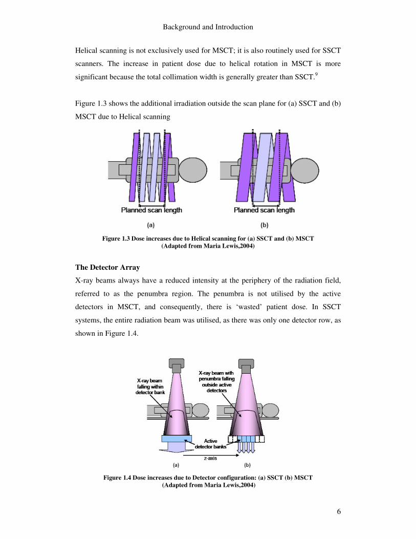
Figure 1.3 shows the additional irradiation outside the scan plane for (a) SSCT and (b)

MSCT due to Helical scanning

Figure 1.3 Dose increases due to Helical scanning for (a) SSCT and (b) MSCT

(Adapted from Maria Lewis,2004)

The Detector Array

X-ray beams always have a reduced intensity at the periphery of the radiation field,

referred to as the penumbra region. The penumbra is not utilised by the active

detectors in MSCT, and consequently, there is ‘wasted’ patient dose. In SSCT

systems, the entire radiation beam was utilised, as there was only one detector row, as

shown in Figure 1.4.

Figure 1.4 Dose increases due to Detector configuration: (a) SSCT (b) MSCT

(Adapted from Maria Lewis,2004)


7

Geometric Efficiency quantifies the utilisation of the detectors for MSCT. Geometric

Efficiency is defined as the ratio of the radiation beam utilised by the detectors to the

total radiation beam.

For SSCT the Geometric Efficiency can be considered to be 100% efficient, while the

efficiency for MSCT scanners can vary. The wasted irradiation to the patient can be

significant, however, as the number of simultaneous slice acquisitions increases the

geometric efficiency improves, as can be seen in Table 1-1 (adapted from Maria

Lewis, 2004).

Table 1.1 Geometric Efficiency for MSCT scanners

Scanner Number and width of acquired Slices (mm)

Total nominal Collimation width (mm)

Z-axis geometric efficiency

4-slice 4 x 1.25 5 66 8-slice 8 x 1.25 10 83 16-slice 16 x 1.25 20 97

1.5.3.2 Changes in Examination Procedures Early conventional SSCT scanners were limited by scan times. Consequently, many

aspects of examination procedures were affected: slow scan times restricted use of the

scanner per patient and as a result minimum volumes were imaged with large slice

widths.

SSCT helical scanning improves both the speed of scan times and the ability to image

thinner slices, however, the x-ray tube heat capacity did not improve significantly and

as a result the examinations were limited by tube current loading. With helical

scanning, the tube is continuously exposing photons, consequently, the tube current

time product is limited to reduce the tube heating.

The advancements in MSCT have dramatically reduced scan times due to sub-second

gantry rotation, while also improving the ability to simultaneously scan multiple

slices. Faster scanning in addition to new tube cooling techniques (STRATON,

Siemens 2004) allow for high tube current values.


8

With the features and possibilities that accompany MSCT, there may be a tendency to

image larger volumes with higher image quality than is needed. This possibility has

been widely noted, as well as the possibility that many scan protocols of MSCT are

not optimized in accordance with the ALARA principle.10 1 11 12 13 14

1.6 Standard Imaging Protocols

Standard protocols used by radiological staff are intended as a benchmark for

individual scan procedures which are then tailored for the specific needs of the

patient. A comparison carried out by the NRPB between patient dose from individual

scan procedures and standard protocols correlated very well.15 An investigative study

of CT techniques also suggested that similar examinations in various Dutch hospitals

were carried out using fixed setting of mAs, kV and slice thickness16. These results

indicate that the standard protocols used in radiological departments provide a very

good basis for the estimation of patient dose for all similar imaging procedures.

The examination protocol used in imaging procedures is the decisive factor that

determines patient dose. Protocols are not set by regulation authorities but are

followed locally in hospitals.

1.6.1 How changes in scan protocols affect patient dose

There are many variables within each examination procedure that influence patient

dose, in particular, slice thickness and the tube current time product (mAs). Slice

thickness and mAs are linked through image noise.

Image noise refers to the random fluctuations in pixel values from a certain mean

level due to both electronic and quantum noise, quantum noise being the dominant

factor. Quantum noise arises from the statistical uncertainty in the finite number of x-

ray photons transmitted in the region of interest, in this case being the individual

slices7. Reducing slice thickness results in less photons incident in this region which

leads to a larger variation of pixel values and subsequently higher image noise.


9

The elevated image noise would reduce the image quality of the resultant image for

clinical diagnosis. To counteract this, the tube current must be increased to reduce the

image noise for thinner slices. The linear relationship between mAs and patient dose

applies, therefore, any increase in the mAs leads to higher patient dose. Indications

are that on average slice thickness for MSCT is reducing leading to higher image

noise than equivalent SSCT examinations7.

1.6.2 Scan Parameters Overview

The main scan parameters of interest for the standard protocols are: Voltage (kVp) Higher peak voltages will result in more x-rays passing through

the body, hence less absorption and patient dose, however,

there is lower image contrast

Tube Current (mA) mAs is directly proportional to patient dose, as tube current

increases, more x-rays are incident onto the patient leading to

higher patient dose

Effective mAs The effective mAs accounts for pitch. mAs divided by the pitch

Slice Collimation (mm) Desired viewing thickness of the tomographic slices

Beam Collimation

(MSCT only)

The product of the number of active detector channels used and

the effective detector row thickness. The number of active

detectors determines MSCT slice thickness. In SSCT the slice

thickness is determined alone by the collimation width

Pitch For MSCT pitch is defined as the table Feed divided by the

beam collimation

Feed The table travel (or movement) per rotation

Tube Rotation (s) Gantry rotation speed


10

1.7 Patient Dosimetry in CT

1.7.1 Introduction

This section provides background information on the patient dosimetry method used

in this project. Evaluation of patient dose is achieved by Thermoluminescence

Dosimetry and the use of an anthropomorphic tissue equivalent phantom. In this

section the radiation quantities used throughout this report are introduced, the

principles behind Thermoluminescence dosimetry, and how this is applied to this

study using diagnostic TLDs are discussed. Other methods of evaluating patient dose

that are relevant to this study are also introduced.

1.7.2 Radiation Quantities

The following radiation quantities are used throughout this study and are in

accordance with the International Commission on Radiation Protection Publication 60

(ICRP 60)17.

Absorbed Dose (D) The absorbed dose, D, is the energy deposited per unit mass of matter and the unit of

measurement is Gray (Gy). One Gray is equivalent to the dose of one joule of energy

absorbed per kilogram of matter (Joule per kilogram). The absorbed dose stated

throughout this study refers to mean absorbed dose over a tissue or organ (or part of)

within the primary radiation field.

Equivalent Dose (H) Absorbed dose does not take into account the type and energy of the radiation causing

the dose; the radiation weighting factors allow for the inclusion of the radiation type

and energy. The radiation weighting factors, wR, are listed in Table 1-2. The weighted

absorbed dose is termed equivalent dose, HT and the equation is expressed as:

� ⋅=R

RTRT DwH ,


11

, where DT,R is the absorbed dose averaged over the tissue or organ T, due to the

radiation R. The unit of equivalent dose is the joule per kilogram with the special

name sievert (Sv).

Table 1.2 Radiation weighting factors Radiation type and energy range

Radiation weighting factor, wR

Photons, all energies 1 Electrons 1 Protons 5 Neutrons ( 10keV-100keV) ( 100keV – 2MeV)

10 20

Alpha particles, fission fragments

20

The only radiation type that will be encountered in this study is photons therefore the

radiation factor needed to determine the equivalent dose is 1.

Effective Dose (E) The relationship between the probability of stochastic effects and equivalent dose is

found to depend on the organ or tissue irradiated. A weighting factor wT is applied to

the equivalent dose to form the effective dose, E.

Table 1.3 Tissue weighting factors

Tissue or organ Tissue Weighting Factor, wT

Gonads 0.2 Bone Marrow (Red)

0.12

Colon 0.12 Lung 0.12 Stomach 0.12 Bladder 0.05 Breast 0.05 Liver 0.05 Oesophagus 0.05 Thyroid 0.05 Skin 0.01 Bone Surface 0.01 Remainder 0.05

The remainder is composed of the following tissues and organs: adrenals, brain, upper large intestine, small intestine, kidney, muscle, pancreas, spleen, thymus and uterus.


12

The weighting factor wT represents the relative contribution of that tissue\organ to the

total detriment, due to these effects resulting from the uniform irradiation of the whole

body. The unit of effective dose is the joule per kilogram with the special name

sievert (Sv). The values of the tissue-weighting factor are chosen to be independent of

the type of energy and of the radiation incident on the body. The tissue weighting

factors are based on the current knowledge of radiobiology.

� ⋅=T

TT HwE

1.7.3 Thermoluminescence Dosimetry

When X-rays are incident on phosphor, secondary electrons that are set in motion

raise valence electrons to a higher forbidden energy level (energy traps). The

electrons stay in these energy traps and the absorbed energy is stored in the phosphor

until the electrons return to the valance shells with the emission of the stored energy

with photons of light.18 When the emission of this light requires stimulation via heat

the process is known as thermoluminescence. The amount of light emitted is

proportional to the amount of radiation absorbed so dose can be measured.

Thermoluminescence is the method used in this study to measure radiation dose.

1.7.3.1 Thermoluminescence Dosemeters (TLDs)

Thermoluminescence Dosemeters (TLDs) are available in many types each with a

range of specifications and shapes. TLDs are available in rods, chips, square rods,

disks and power form.

Lithium Fluoride is the most commonly used material in Thermoluminescence

Dosimetry. TLD 100 chips doped with magnesium (Mg) and titanium (Ti)

(LiF:Mg,Ti) have a range of 10 µ Gy to 10Gy and have a linear response from .1mGy

to 10mGy19. TLD 100 chips are commonly used in personal and radiotherapy

dosimetry.

TLD 100H chips are Lithium Fluoride doped with Mg, Cu and P (LiF:MCP) to give

some advantageous features over other chips such as TLD 100: TLD 100H chips are


13

highly sensitive giving a range of 1�Gy to 10Gy and also thermal fading1 is

negligible. As with most Lithium Fluoride TLDs the effective atomic number is 8.2

giving almost tissue equivalent properties - the effective atomic number of tissue is

7.420. The chip dimensions of each TLD 100H are 3.2 x 3.2 x .38 mm20. TLD 100H

chips are used in this study to measure radiation dose.

1.7.4 Patient dose measurement

Patient dose will be measured for the standard imaging protocols using

thermoluminescence dosimetry and a tissue equivalent Humanoid phantom. The

methodology used to measure and evaluate patient dose is discussed in Chapter 2.

1.7.5 Other Methods of Evaluating Patient Dose Apart from thermoluminescence dosimetry, other less time consuming methods can

also be used to measure patient dose. These methods are relevant for comparison of

the method used in this study. The following are common dosimetry quantities used to

evaluate patient dose in CT

1.7.5.1 Dosimetry Quantities

Computed Tomography Dose Index (CTDI): The principle dosimetry quantity

used for evaluation of dose in CT is the Computed Tomography Dose Index (CTDI)

and is calculated from the dose profile. The CTDI is defined as the integral along a

line parallel to the axis of rotation (z) of the dose profile (D(z)) for a single slice

divided by the nominal slice thickness T21:

�+∞

∞−

= dzzDT

CTDI )(1

(mGy)

CTDI is the integral of the dose along the infinite z-axis from a single slice divided by

the nominal slice thickness. It is measured with a 100mm long pencil ionization

chamber. Figure 1.5 shows a typical dose profile of a CT scanner measured at

isocentre.

1 Fade is the loss of the stored signal over time. It can be caused by exposure to light or heat. The use of a pre-read anneal can reduce the effects of fade by eliminating the transient peaks that are the most susceptible to fading


14

Figure 1.5 Dose Profile of CT scanner

CTDIw: The weighted CTDI is an estimate of the average dose over a single slice in

CT dosimetry phantom and is used to compare dosimetry performance against a

reference dose value in order to optimize patient protection.

pcw CTDICTDICTDI ,100,100 3/23/1 += (mGy)

, where cCTDI ,100 and pCTDI ,100 are measured by the 100mm active length pencil

beam ionization chamber at the central and peripheral regions of a cylindrical Perspex

phantom respectively.

CTDIvol: The volume CTDIw describes the average dose over the total volume

scanned in a sequential or helical slice

CTDIvol = FactorPitch CT

CTDI W (mGy)

DLP: Dose Length Product (mGy cm) is a dose descriptor used as an indicator of

overall exposure for a complete CT examination in order to allow comparison of

performance against a dose value.

� ••=i

w NTCTDIDLP (mGy cm)

,where T is the slice thickness and N is the number of slices.


15

1.7.5.2 Monte Carlo Method

This method of measuring patient organ dose involves CTDIw and Monte Carlo data

tables. The data tables were generated using a Monte Carlo technique which simulates

the passage of radiation through the patient anatomy22. The anatomy of the patient is

approximated by a mathematical model of the body using geometrical shapes, the

Medical Internal Radiation Dosimetry (MIRD) phantom. The Monte Carlo dose

simulation was carried out with a range of CT scanners available at the time of the

survey (1989)23 using scan parameters for adult phantoms. The effective patient can

subsequently be calculated by means of tissue weighting factors (See Section 1.7.2)

Only a limited number of CT scanners were available in the period when the Monte

Carlo simulation tables were being generated, and multislice CT scanners were not

yet available. Consequently effective dose estimation of modern scanners has to rely

on best fitting MSCT scanners to the older data. Monte Carlo simulations have been

reported to under estimate patient dose by up to 18%24. This method however is not

time consuming as the organ and effective dose can easily be calculated using readily

available spreadsheets.

1.7.5.3 DLP Method DLP (See Section 1.7.5.1) will not give an indication of organ dose but the effective

dose can be estimated, however, by calculation of the product of the DLP and EDLP,

the normalized effective dose values, for different regions of interest. Table 4 shows

EDLP values from the NRPB for the calculation of adult effective dose.

Table 1.4 EDLP - normalized effective dose values for adult DLP values Region of Body

EDLP, Adult [mSv mGy-1 cm-1]

Head/Neck 0.0031 Head 0.0021 Neck 0.0059 Chest 0.014 Abdomen/Pelvis 0.015 Trunk 0.015


16

1.8 Guidelines on Quality Criteria for CT

There are no standard regulations to restrict dose levels in diagnostic CT imaging,

however, CT imaging does fall under the ICRP publication 60 (1991) which aims to

keep medical exposure in line with the ALARA principle (to keep exposure as low as

reasonably achievable) and also to justify exposure levels. There are two guidelines

on quality criteria for CT examinations. The objectives of the guidelines are to

provide:

• Adequate image quality, comparable throughout Europe

• Reasonable low radiation dose per examination

European Commission (1999) Eu 16262 EN: European guidelines on quality

criteria for computed tomography25

The EU 16262 European guideline presents detailed examples of ‘Good Imaging

Techniques’ for various different examination procedures to minimize unnecessary

patient exposure. Many factors contribute to the variation in patient dose, in

particular, the local scanning protocol. The guidelines acknowledge that this factor is

quite significant.

The European Commission regulatory body recommends the use of dose reference

levels to minimise patient dose exposure in similar examinations. These reference

levels are not intended to be applied individually, mean patient exposure levels that

are above the reference level should prompt an investigation into the reason for this.

The diagnostic reference levels (DRL) given for standard examination are the CTDIw

(mGy) and the Dose Length Product (DLP) (mGy cm).

2004 CT Quality Criteria26

MSCT technology has developed greatly since 1999 and new guidelines primarily for

MSCT have evolved from a new study. The diagnostic reference levels no longer

include CTDIw or DLP, the only dosimetry quantity given is the CTDIvol

recommendation. The DLP can be calculated however by the product of the

recommended CTDIvol and the length of the scan procedure.


17

1.9 Radiation Risks

The risk of inducing a fatal cancer in a lifetime is estimated to be .05 per Sievert by

IRCP 60 (1991) for low doses, such as in diagnostic CT. Doses from diagnostic CT is

in the range of mSv, which is 0.00005 per mSv. This equates to a fatal cancer risk of 1

in 20,000 for every 1mSv radiation dose. This risk is age related, and as the age of the

patient increases the risk factor becomes less significant.

These cancer risks are based on the linear no threshold model (LNT) hypothesis of

radiation. The risk ratios are based on high dose exposures (atomic bomb survivors at

Hiroshima and Nagasaki) extrapolated (linearly) down to much lower levels, to zero

dose. The hypothesis postulate that even the smallest dose has a risk associated with

it, as no threshold exists below which there is no radiation risk.

1.10 Summary

MSCT technology is now in common clinical use and the frequency of CT imaging is

continually increasing. This increase has led to due concern regarding increases in

patient dose from CT examinations. The increases in patient dose can be related to

technology advancements in MSCT and the subsequent changes in practice. Patient

dose in this study will be estimated by means of Thermoluminescence dosimetry and

a tissue equivalent phantom.

Experimental Methods and Materials

18

2 Experimental Methods and Materials

2.1 Introduction

The objective of this study is to evaluate patient dose using an anthropomorphic

phantom and diagnostic TLDs. This chapter outlines the experimental methods used

to achieved this aim and also outline the materials used.

Diagnostic TLDs are used within the humanoid phantom to measure the radiation

dose absorbed by the patient. Procedures employed to measure the radiation dose of

the TLDs are outlined in Section 2.2, in addition to the preparation of the TLDs prior

to their use for measurement of absorbed dose.

The anthropomorphic phantom used in the study is also detailed in Section 2.3. A

major part of this study was to develop a clear means of estimating patient dose using

the phantom. The methodology used to provide this is detailed in Section 2.4.

The various CT scanners used to measure patient dose and the standard protocols

performed on the phantom are detailed in Section 2.5.


19

2.2 Thermoluminescence Dosemeters Setup

2.2.1 Introduction

45 TLD 100H square chips, as described in Section 1.7.3.1, were purchased from

QADOS UK. The procedure to use the TLDs to measure radiation dose involved a

number of routine steps to measure the irradiated dose to the TLD.

• Irradiation

• Annealing & Cooling

• Readout Cycle

In addition, the TLD reader had to be calibrated for use with the TLD 100H chips.

This involved a process to determine the Reader calibration factor (RCF) to assess the

linear relationship between the readout of the TLD 100H chips in nanocoloumbs and

the radiation dose received. In addition an Element Correction Coefficient (ECC) for

each specific TLD was determined to account for variations within a batch of TLD

chips

.

2.2.2 Handling of TLDs

Vacuum tweezers are recommended when handling the TLD chips in order to avoid

foreign deposits, scratches or loss of mass of the chips. Vacuum tweezers (Charles

Austen Pumps Ltd., Model DYMAX 30) were used in all handling of the TLD chips,

unless the use of mechanical tweezers was unavoidable.

2.2.3 Irradiation

During the TLD calibration process, irradiation of the TLD took place under the same

conditions. Exposure was carried out using a Castor x-ray generator. The procedure

for exposure was as follows:

• X-ray generator switched on

• X-ray generator warmed up


20

• TLD 100H chips placed in perspex holder at 100cm from the x-ray tube in

centre of radiation field. Perspex holder placed on foam to reduce backscatter

from the couch. The perspex holder shown in Figure 2.1(a).

• Field size set ( was kept consistent for all readings)

• Dose readings from x-ray tube taken before and after TLD irradiation at

Perspex centre location (with TLDs and holder behind a protective barrier)

• TLDs irradiated

• X-ray generator switched off

The dosemeter used to measure the exposure from the x-ray tube was a calibrated

solid state detector, the SOLIDOSE Digital Dosemeter, Model 400 from RTI

Electronics, Figure 2.1(b). Although irradiation of the TLD chips was done above the

couch, backscatter was still evident, which the solid state detector did not account for,

separate backscatter measurements had to be taken.

(a) (b)

Figure 2.1 a) Perspex Holder and (b) Dosemeter


21

2.2.4 Annealing & Cooling

Annealing of the TLDs is needed to completely remove any remaining electrons in

the energy traps. Annealing was done in an oven (Carbolite, Eurotherm 2408 CP,

Model TLD/3), shown in Figure 2.2. The recommended annealing procedure for TLD

100H chips involves heating to a temperature of 240°C maintained for 10 minutes.27

The full annealing programme used for the oven can be found in Appendix I. This

annealing procedure was used prior to each irradiation of the TLD chips. The

annealing steps are listed below:

• Turn on oven

• Place TLD in thin oxidised aluminium annealing container (Qados, UK)

• Place in oven rack

• Set annealing programme (see Appendix I)

• Run programme

The annealing temperature of 240°C could not be exceeded as this would decrease the

sensitivity of the chips, a secondary maximum limiting oven sensor could be

independently set to ensure the maximum temperature was not breached.

After the initial programme was finished the TLD chips were then allowed cool to

room temperature in the oven as part of the annealing programme. Another more

rapid cooling process has been recommended to increase sensitivity of the TLDs,

where the cooling process takes place outside of the oven28 29. However, the

reproducibility of this method was not guaranteed for each annealing process.

2.2.5 TLD Readout

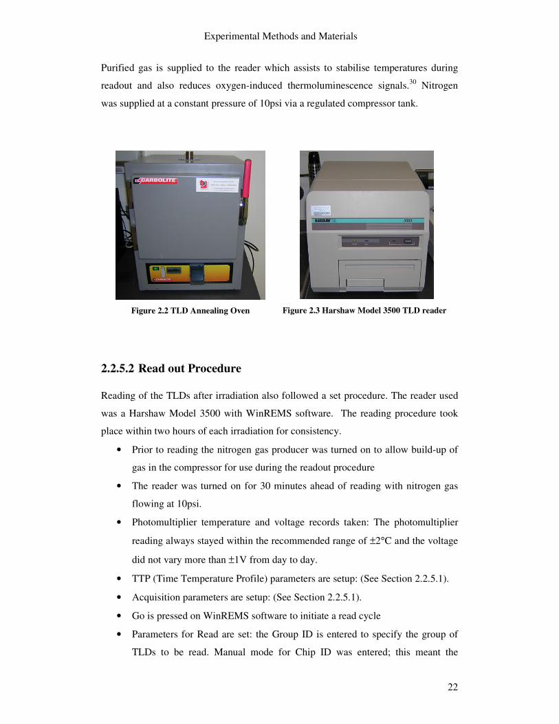
2.2.5.1 TLD Reader

The TLD reader used was a Harshaw Model 3500, as shown in Figure 2.3. The reader

is controlled via a PC interface running WinREMS software. The reader consists of a

drawer containing a planchet capable of a holding single TLD, a Read button and

LED indicator. The planchet is heated releasing the electrons (via

thermoluminescence) captured during the irradiation process which are then detected

by the photomultiplier tube (PMT) and amplified.


22

Purified gas is supplied to the reader which assists to stabilise temperatures during

readout and also reduces oxygen-induced thermoluminescence signals.30 Nitrogen

was supplied at a constant pressure of 10psi via a regulated compressor tank.

Figure 2.2 TLD Annealing Oven

Figure 2.3 Harshaw Model 3500 TLD reader

2.2.5.2 Read out Procedure Reading of the TLDs after irradiation also followed a set procedure. The reader used

was a Harshaw Model 3500 with WinREMS software. The reading procedure took

place within two hours of each irradiation for consistency.

• Prior to reading the nitrogen gas producer was turned on to allow build-up of

gas in the compressor for use during the readout procedure

• The reader was turned on for 30 minutes ahead of reading with nitrogen gas

flowing at 10psi.

• Photomultiplier temperature and voltage records taken: The photomultiplier

reading always stayed within the recommended range of ±2°C and the voltage

did not vary more than ±1V from day to day.

• TTP (Time Temperature Profile) parameters are setup: (See Section 2.2.5.1).

• Acquisition parameters are setup: (See Section 2.2.5.1).

• Go is pressed on WinREMS software to initiate a read cycle

• Parameters for Read are set: the Group ID is entered to specify the group of

TLDs to be read. Manual mode for Chip ID was entered; this meant the


23

individual chip ID was entered manually before each read. Alternatively, the

chips read cycle could be automated to a predefined sequence.

• Each TLD is placed on the planchet in the tray of the reader, the chip ID

entered manually and ‘READ’ is pressed on the Harshaw reader.

• At predefined intervals PMT noise and Light reference readings are taken.

• Intermittently between readings the background reading is taken manually,

this is done with no TLD on the planchet as recommended by the manufacture.

The average of the background readings was subtracted from the TLD

readings.

• TLD readings are exported as a text file, which can then be imported into a

excel sheet for analysis.

2.2.5.3 TTP and Acquisition Set-up

TTP

Time Temperature Profile (TTP) defines the temperature to which the TLD is heated

to as a function of time. Various TTP setup can be programmed with the WinREMS

software. Each TLD type has specific TTP setup parameters to define how the TLD is

heated as a function of time for analysis by the TLD reader. The TTP setup for TLD

100H chip is shown in Table --.

Table 2.1 TTP setup parameters for TLD 100H chips Mode PreHeat Acquire Anneal Temperature (oC) 100 240 240 Time (sec) 0 36.66 0 Temperature Rate (oC/sec) n\a 4 n\a

This TTP setup was used throughout the readout of all TLD 100H chips. No

annealing is done with the Harshaw TLD reader.

Acquisition Setup

The acquisition setup includes parameters on the measurement of the TLDs such as

the mode of acquisition, calibration factors applied and PMT/Light reference reading

interval rate. The full list of the acquisition setup parameters for each of the various

modes can be found in Appendix I.


24

2.2.5.4 PMT noise and Light reference levels

The PMT noise and Reference Light levels were taken at intervals set in the

Acquisition parameters. The values of these should remain reasonably consistent

during readings.

PMT Noise

PMT noise readings measure the background noise in the system due to light leaks.

To take the PMT noise reading, the tray of the reader was placed in the ‘between’

position as far in as possible without the drawer being in the ‘closed’ position. The

read button was pressed and the reading was taken for 10 seconds.

Light Reference Levels

The Reference Light measures the output from LED reference lights to produce a

constant light output. The reference lights are located within the PMT Assembly. To

take the reading, the drawer was placed in the ‘open’ position and the read button was

pressed. The duration of the reading was for 10 seconds.

2.2.6 Reader Calibration

2.2.6.1 Introduction

The aim of calibrating the reader was to determine the relationship between the

absolute readings of nanocoloumbs (from the TLD reader) and the TLD irradiated

dose. This relationship was determined by way of a Reader Calibration Factor (RCF)

and also by Element Correction Coefficients (ECCs).

RCF: The RCF relates the charge value outputted by the PMT in nC to the actual

irradiated dose given to the TLD. The RCF is applied on the basis of the TTP

selected.

ECC: The response of TLD can vary widely within each batch of TLDs, to account

for this Element Correction Coefficients (ECCs) are applied for each TLD separately.


25

The TLD reader calculates the readout of the each TLD by the following equation.

Exposure (�Gy) = ECC x Charge (nC)

RCF (nC/�Gy)

2.2.6.2 Reader Calibration Method

Calibration of the reader involved a number of fixed steps which are documented in

detail in the operator’s manual of the Harshaw TLD Reader. A summary of the steps

taken are detailed below. Prior to each irradiation of the TLDs, annealing took place.

Also, it should be noted that each TLD had to be tracked individually as specific ECC

values were applied during calibration processes.

• Selection of Calibration TLDs

o TTP parameters setup

o Acquisition parameters setup for ‘Generate Calibration Dosimeters’

o TLD 100H chips were irradiated and subsequently readout.

o Generate Calibration Dosimeters Dialog Box opened

o Field limits of (+/- 10%) selected

o ECC values calculated for each chip

o TLD with readout values closest to the mean of the population were

selected as calibration chips

o Calibration chips and ensuing ECC values were accepted to ECC

database


26

• Calibration of Reader

o TTP parameters setup

o Acquisition parameters setup for ‘Calibrate Dosimeters’

o Calibration chips were irradiated to known dose in mGy

o Readout of calibration chips

o ECC values applied to calibration chips during readout

o ‘Reader Calibration’ Dialog Box opened

o Known irradiated dose entered (�Gy)

o Reader Calibration Factor (RCF) calculated

o RCF accepted into database for specific TTP used

For all future reading using the same TTP, as stated during the calibration

proceedings, the RCF will be applied to give the PMT output reading in Gy rather

than in nanocoloumbs. The complete acquisition setup parameters for each stage of

calibration are detailed in Appendix I.

2.2.7 Field Dosimeters Calibration

Following the reader calibration the TLD 100H dosimeters to be used in the

experiments were calibrated. This calibration procedure determined separate ECC

values for each TLD. Prior to irradiation of the TLDs annealing took place

• TLDs irradiated to known dose

• Calibrated TTP selected

• Acquisition parameters setup for ‘Calibrate Field Dosimeters’

• TLDs were readout

• Dosimeter Calibration dialog box was opened

• Known irradiated dose entered (�Gy)

• Field limits of (+/- 15%) selected

• ECC for each TLD calculated

• ECC values accepted into ECC database

After this procedure the TLD 100H chips were ready to be used to measure radiation

dose.


27

2.2.8 Linearity of Field Dosimeters

The field dosimeters should be calibrated using an exposure that is within the range of

their proposed use. TLD 100H chips have very good linearity in the diagnostic energy

ranges (up to 20mGy)31 The range of dose values for diagnostic CT is between

0.1mGy and 30mGy and the linearity of the dosimeters was evaluated for this range.


28

2.3 Anthropomorphic phantom

The RANDO® Phantom is constructed with a natural human skeleton which is cast

inside soft tissue-simulating material. Lungs are moulded into to the contours of the

natural ribcage. The phantom is sliced into 35 axial slices, slice 1-34 are 2.5cm

thickness and slice 35 is 9.5cm thick.

Two tissue-simulating materials are used to construct the RANDO® Phantom, soft

tissue material and lung material. The soft tissue material is manufactured with a

propriety urethane formulation. The material has an effective atomic number and

mass density that stimulates muscle tissue with randomly distributed fat. The lung

material has the same effective atomic number as the soft tissue material with a

density that simulates lungs in a median respiratory state.32

Figure 2.4 RANDO® Phantom

Hole grid patterns are drilled into slice 1-34 to enable insertions of dosimeters. Hole

grids are not drilled through bone. The holes are filled with standard plugs. Figure 2.4

shows the complete RANDO® Phantom in its assembly unit and also Slice 12 of the

phantom, where the hole grids can be seen and also the tissue and lung simulating

material.


29

2.4 Organ Measurement

2.4.1 Introduction

Accurate organ dose measurement is a key focus of evaluating patient dose for the

standard examination protocols. The method employed to evaluate patient dose in this

study used a Humanoid phantom and diagnostic Thermoluminescence Dosemeters

(TLDs). To accurately measure the absorbed radiation dose, each organ must be

located correctly within the phantom.

This section covers the following areas:

• Selection of measurement organ

• Distribution of TLDs within organs

• Location of organs within humanoid phantom


30

2.4.2 Organ Selection

Organs were selected based on recommendations by the International Commission on

Radiation Protection Publication 60 (ICRP 6033). The effective dose can be calculated

by way of tissue weighting factors, wT, for the measurement organs (Section 1.7.2).

The tissue weighting factors are shown in Table 2-2.

Table 2.2 Tissue Weighting Factors

Tissue or organ Tissue Weighting Factor Gonads 0.2 Bone Marrow (Red) 0.12 Colon 0.12 Lung 0.12 Stomach 0.12 Bladder 0.05 Breast 0.05 Liver 0.05 Oesophagus 0.05 Thyroid 0.05 Skin 0.01 Bone Surface 0.01 Remainder 0.05

The remainder is composed of the following tissues and organs: adrenals, brain, upper large intestine, small intestine, kidney, muscle, pancreas, spleen, thymus and uterus.

Each of the main organs (Table 2-2) was selected for measurement excluding the

female gonads and breast. Two remainder organs were also selected for measurement

of absorbed radiation dose, the brain and kidneys. In addition, the absorbed dose to

the lens of the eye was also measured using two TLDs.


31

2.4.3 Distribution of TLDs

A finite of number of TLDs were used to measure the radiation dose to the organs.

The distribution of the TLDs was based on similar investigations. M Law et al (2003)

noted that at least two TLD’s should be used for each organ of interest, to allow for

variations and errors in the TLDs34. Groves et al (2004) concluded that a minimum of

three TLDs should be used with some exceptions such as the gonads and thyroid35.

Organ size also was a factor when determining the distribution of the TLDs.

The distribution of the TLDs used is shown in Table 2-3. The dose measurements of

bone marrow (red) and bone surface were made using the same TLDs.

Table 2.3 TLD Distribution in Organs Tissue or organ Head Protocol Chest Protocol Abdomen Protocol Gonads 2 2 2 Bone Marrow (Red) 4 5 5 Colon 4 4 4 Lung 6 6 6 Stomach 4 4 4 Bladder 2 2 2 Liver 4 4 4 Oesophagus 4 4 4 Thyroid 2 2 2 Skin 3 4 4 Bone Surface - - - Brain 2 2 2 Eye 2 2 2 Kidneys 2 2 2 Total 41 43 43

The placement of each individual TLD was kept consistent for each examination to

minimize any error.


32

2.4.4 Placement of TLDs

To measure the absorbed dose in each organ, precise placement of the TLDs within

the phantom was needed.

As previously mentioned only lung, tissue and bone structures are visible within the

anthropomorphic phantom, these alone did not provide sufficient information to

locate each of the organs of interest. A clear methodology was needed to provide a

transparent and accurate way of locating each organ within the phantom.

Organ location for the phantom included two stages

• Analysis of the phantom skeleton structure

• Analysis of human body structure


33

2.4.4.1 Analysis of Phantom Structure

Firstly, a whole body CT image of the phantom was obtained using the Phillips

ACQSim RT scanner; this can be seen in Figure 2.5. This image was then imported

into ImageJ36, an image processing and analysis tool shown in Figure 10.

Figure 2.5 ImageJ Software Tool

From the CT image, the length of the CT phantom was determined to be 910mm.

Using the ‘Analyze – Set Scale’ command within ImageJ (see Figure 2.5), the length

of a selected line is given in pixels, the known distance and unit length can then be

entered to scale the image. The scale set for the image used was 0.533 pixels/mm.

Subsequently any point to point distance on the image was known.


34

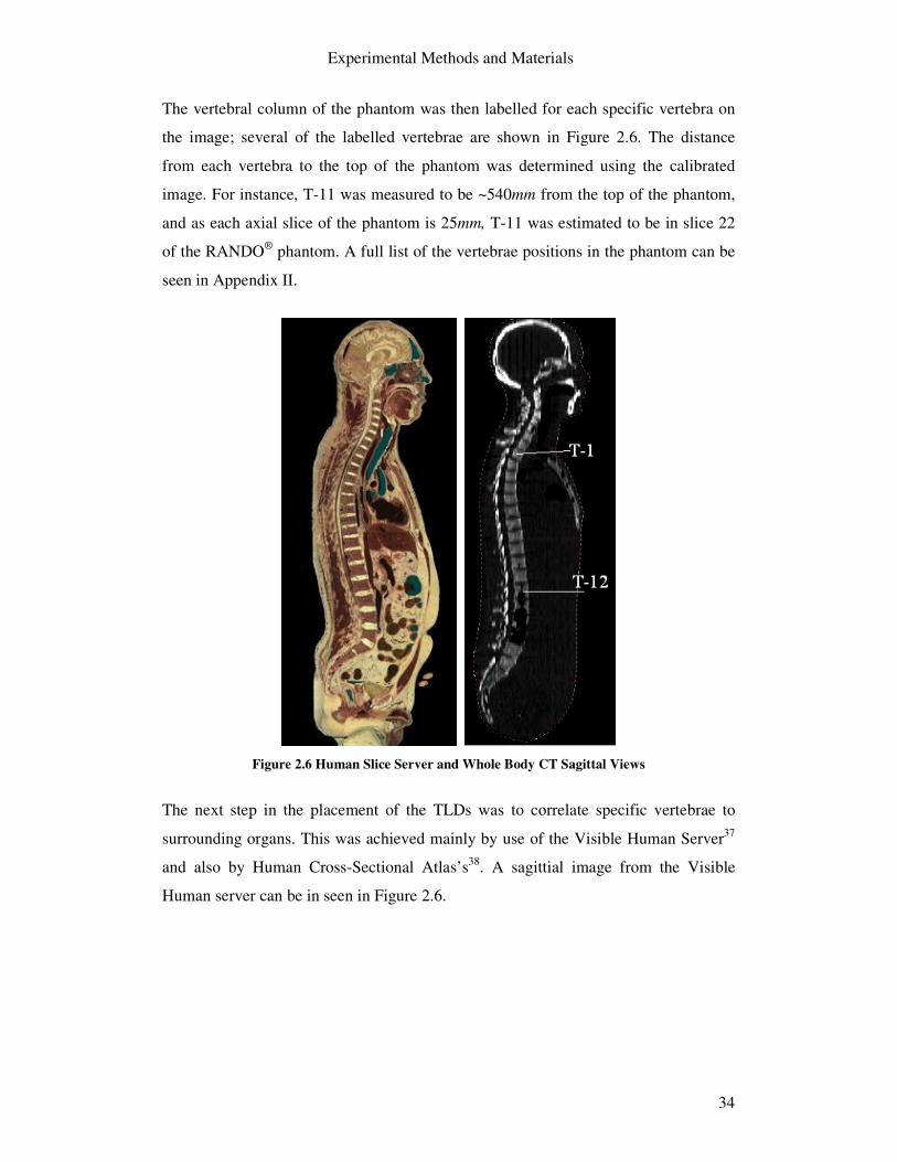
The vertebral column of the phantom was then labelled for each specific vertebra on

the image; several of the labelled vertebrae are shown in Figure 2.6. The distance

from each vertebra to the top of the phantom was determined using the calibrated

image. For instance, T-11 was measured to be ~540mm from the top of the phantom,

and as each axial slice of the phantom is 25mm, T-11 was estimated to be in slice 22

of the RANDO® phantom. A full list of the vertebrae positions in the phantom can be

seen in Appendix II.

Figure 2.6 Human Slice Server and Whole Body CT Sagittal Views

The next step in the placement of the TLDs was to correlate specific vertebrae to

surrounding organs. This was achieved mainly by use of the Visible Human Server37

and also by Human Cross-Sectional Atlas’s38. A sagittial image from the Visible

Human server can be in seen in Figure 2.6.


35

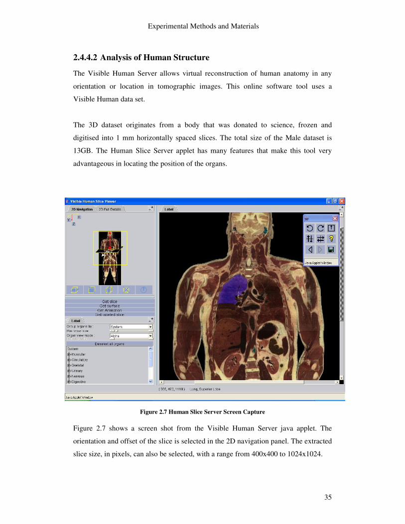
2.4.4.2 Analysis of Human Structure

The Visible Human Server allows virtual reconstruction of human anatomy in any

orientation or location in tomographic images. This online software tool uses a

Visible Human data set.

The 3D dataset originates from a body that was donated to science, frozen and

digitised into 1 mm horizontally spaced slices. The total size of the Male dataset is

13GB. The Human Slice Server applet has many features that make this tool very

advantageous in locating the position of the organs.

Figure 2.7 Human Slice Server Screen Capture

Figure 2.7 shows a screen shot from the Visible Human Server java applet. The

orientation and offset of the slice is selected in the 2D navigation panel. The extracted

slice size, in pixels, can also be selected, with a range from 400x400 to 1024x1024.


36

Once the slice is pre-selected from the 2D navigation panel, “Get labelled slice” will

retrieve the relevant information from the dataset located in various servers. The

selected slice will be displayed in full size. By highlighting various parts of the

selected image, using a mouse-over, the part name is displayed. Figure 2.7 shows the

superior lobe of the right lung highlighted.

Figure 2.8 shows an axial slice obtained from the Human Slice server displaying the

11th thoracic vertebra, the liver and the stomach. Slice 22 of the RANDO® phantom

contains T-11 as estimated previously, see Figure 2.8. Using these two images,

appropriate locations for measurement of the stomach and liver are evident.

Human Server Axial Slice Slice 22

Figure 2.8 Organ Placement Method

A full list of the images used and the corresponding phantom slice images with the

TLD positions marked can be found in Appendix II for each organ considered for

measurement.


37

While human anatomy is consistent, the precise structure and location of organs can

differ between individuals. Consequently, the human slice server dataset used to

construct the axial images shown above is specific to one individual, as is the with the

RANDO® phantom used to assess patient dose. However, the images correlated well

subsequently a very accurate estimation of the organ location within the phantom was

possible. When possible, bone structures were also used to confirm the location of

organs.

2.4.4.3 Additional Organ Placement Methods

The site of measurement for skin and red bone marrow could not be determined using

the method outlined previously. The location of these organs varied for each

examination protocol to ensure they were within the primary imaging volume. The

other organ locations remained constant throughout the examination procedures.

Skin Measurement

To measure the adsorbed dose to the skin, the TLDs were placed on different slices

within the primary radiation field, at the front, side and back of the RANDO®

phantom.

Red Bone Marrow Measurement

Red bone marrow measurement proved to be difficult as unlike other tissues or

organs, there is no unambiguous place within the RANDO® phantom for the

measurement of absorbed dose. Also holes are not provided in bone structures.

Red bone marrow is found in sternum, vertebrae, ribs, clavicles, pelvis, long bones

and skull and produces red blood cells and special white blood cells called

lymphocytes and other elements of blood such as platelets39. Cohnen et al (2001)

measured bone marrow in several locations including clavicle, sternum, ribs, thoracic

and lumbar vertebrae and pelvis, when investigating the radiation exposure resulting

from a Multi-Slice CT of the heart40. In this study bone marrow was measured in the

clavicle, sternum, ribs, vertebrae and pelvis (iliac crest). The exact positioning of the

TLDs for bone marrow can be seen in Appendix II.


38

2.4.5 Summary

Although there is much detailed literature dedicated to organ measurement in

accordance with ICRP 60 recommendations, information is not available on precise

placement of measurement devices within Humanoid phantoms. This is not a

significant problem if due consideration is given to location of the organs, however,

comparisons between similar studies can be uncertain especially in the case of red

bone marrow.

The methodology developed during this study of patient dose is a transparent means

of providing an accurate estimation of patient organ dose using a RANDO® phantom.

The method developed can easily be adopted and applied to similar studies of organ

dose.


39

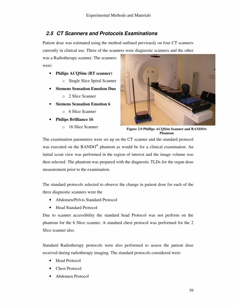
2.5 CT Scanners and Protocols Examinations

Patient dose was estimated using the method outlined previously on four CT scanners

currently in clinical use. Three of the scanners were diagnostic scanners and the other

was a Radiotherapy scanner. The scanners

were:

• Philips ACQSim (RT scanner)

o Single Slice Spiral Scanner

• Siemens Sensation Emotion Duo

o 2 Slice Scanner

• Siemens Sensation Emotion 6

o 6 Slice Scanner

• Philips Brilliance 16

o 16 Slice Scanner

The examination parameters were set up on the CT scanner and the standard protocol

was executed on the RANDO® phantom as would be for a clinical examination. An

initial scout view was performed in the region of interest and the image volume was

then selected. The phantom was prepared with the diagnostic TLDs for the organ dose

measurement prior to the examination.

The standard protocols selected to observe the change in patient dose for each of the

three diagnostic scanners were the

• Abdomen/Pelvis Standard Protocol

• Head Standard Protocol

Due to scanner accessibility the standard head Protocol was not perform on the

phantom for the 6 Slice scanner. A standard chest protocol was performed for the 2

Slice scanner also.

Standard Radiotherapy protocols were also performed to assess the patient dose

received during radiotherapy imaging. The standard protocols considered were:

• Head Protocol

• Chest Protocol

• Abdomen Protocol

Figure 2.9 Phillips ACQSim Scanner and RANDO® Phantom


40

2.6 Summary

The experimental methods to assess patient dose using an anthropomorphic phantom

and diagnostic TLDs are described in this section.

The preparation and use of TLD100H chips are outlined in Section 2.2. A key part of

this thesis was the development of a method to assess organ dose using the RANDO®

phantom, which is described in Section 2.3. The methodology used to achieve this is

described in Section 2.4. The CT scanners used and the standard protocols are

outlined in Section 2.5.

Results and Discussions

41

3 Results and Discussions

3.1 Introduction

The results from the standard imaging protocols, the Abdomen/Pelvis, Head and

Chest protocols, for the various models of CT scanners are the main focus of this

section.

The standard imaging protocols were performed on the RANDO® Phantom with the

diagnostic TLDs in place within the phantom for organ measurement. Each TLD was

then read out as and the results were imported into an excel sheet where the average

dose to each organ and the effective dose for each imaging procedure was calculated

in accordance with ICRP 60.

The standard imaging protocols will be presented and discussed under three headings:

1. Scan Parameters and Comparison with Imaging Guidelines

The standard protocols are presented and compared with international

guidelines on Quality Criteria in CT imaging

o The European Guidelines on Quality Criteria for Computed

Tomography, 1999 (EU 16262)

o 2004 CT Quality Criteria (MSCT 2004)41

2. Measured Organ Dose

o The average absorbed dose to each of the organs is presented from

measurements by the TLDs within the phantom. The absorbed dose

is averaged over the organ (or part of) located within the primary

radiation field or as affected by scatter radiation.

o A legend accompanies each table of results to show which organs

were fully located in the primary radiation beam, the organs which

were partly in the radiation beam or the organs only affected by

scatter.


42

3. Effective Dose and Risk Factors

o The effective dose is calculated from the organ dose for each of the

protocols in accordance with ICRP 60 to allow for direct

comparison between protocols. The associated risk factors for each

protocol are also calculated in accordance with ICRP 60.

The diagnostic protocols are then discussed with regard to both patient dose guidance

levels and typical patient dose levels for similar investigations presented in the

literature. Patient dose was also measured for radiotherapy protocols and these results

will also be presented.

Analysis of the TLD calibration results are first discussed in Section 3.2.


43

3.2 TLD Analysis

The TLD reader was assigned a RCF factor for the batch of TLD 100H chips. The

RCF was .188 (nC/�Gy). Each chip was also assigned EEC values. The

reproducibility of the TLDs was evaluated three exposures was found to be within 5%

(mean relative standard deviation) with a max of 5.73 and a min of 1.33%.

The TLD chips were 5.27% of the mean batch response, however, with a max of

15.46% and a min of 0.012%. PMT noise and Light reference levels remained

constant throughout the project.

The TLD variation could be accounted for by a number of reasons,

• the castor x-ray generator symmetry,

• dosemeter reading and also the

• TLD reader.

All TLDs were calibrated using an x-ray generator using similar kV settings and mA

settings but the TLDs are used to measure exposures from a CT scanner. It is not

known what inaccuracies this may have brought to the TLD readings. A CT scanner

could have been used to expose and calibrate the TLDs as stated by A M GROVES et

al (2004)24. Also an ion chamber would be better suited to measure the TLD exposure

than a solid state detector as this inclusively accounts for backscatter.

The Linearity of the TLD 100H chip was also evaluated and can be seen in Figure 3.1.

The TLD calibration results can be seen in Appendix I.

Figure 3.1 TLD 100H linearity

Linearity of TLD 100H

0

5

10

15

20

25

30

35

0 5 10 15 20 25 30 35

Irradiation [mGy]

Mea

sure

d [m

Gy]


Linear Scale


44

3.3 Diagnostic Protocols

3.3.1 Abdomen/Pelvis Protocol

The main protocol examined for each of the three diagnostic scanners was the

Abdomen/Pelvis protocol. This protocol was easily comparable as the scan length

parameter for each of the scanners’ standard protocol was very similar. Table 3-2

below shows the standard protocol for each of the scanners.

Table 3.1 Abdomen/Pelvis Protocol Parameters

2 Slice 6 Slice 16 Slice Spiral Spiral Spiral kV 130 130 120 Effective mAs 63 95 200 Slice thickness (mm) 8 5 5 Scan time 17.09 17.35 11.61 No. of slices 51 82 81 Scan length (mm) 408 410 405 Feed (mm) 20 15 28.8 Collimation 2x4mm 6x2mm 16x1.5mm Tube Rotation (s) .8 .6 .75

The main parameters to note are the effective mAs and also the slice thickness. It is

important to note the decrease in slice thickness from 8mm to 5mm. While the 6 and

16 Slice scanner’s slice thickness is consistent at 5mm, the 16 slice scanner’s effective

mAs is over twice that of the 2 slice scanner: it would be expected that this substantial

increase in effective mAs would result in higher quality images.


45

3.3.1.1 Comparison with EU Guidelines

There are no guideline for the imaging of both the abdomen and pelvis in one scan in

the EU 16262 guidelines (See Section 1.8). The recommendations for the parameters

of interest for the routine Abdomen and also the routine Pelvis are given in Table 2

below. Also recommended in the guidelines are the CTDIw and DLP for the routine

procedures. MSCT 2004 (See Section 1.8) guidelines are also presented

Table 3.2 General Abdomen and Pelvis Guidelines Parameter Guideline (EU 16262) -

Abdomen Guideline (EU 16262) -

Pelvis Guideline (MSCT 2004)

Abdomen/Pelvis X-ray tube Voltage (kV)

Standard Standard Medium (110-130kV)

Tube Current Time Product (mAs)

Should be as low as consistent with required image quality


Adjusted to patient size

Nominal Slice Thickness

7-10mm; 4-5mm for dedicated indications only

7-10mm; 4-5mm for suspected small lesions

1-2.5mm

Protective Shielding

Lead purse for male gonads if radiation field is less than 10-15cm away

Lead purse for male gonads

-

Pitch 1.0 1.0 0.9-1.3 CTDIw 35 mGy 35 mGy - DLP 780 mGy cm 570 mGy cm - CTDIvol - - <15mGy

EU 16262 guidelines recommend the use of protective shielding for both the abdomen

and pelvis routine procedures. Protective shielding is not specified in the MSCT 2004

guidelines. The slice thickness has substantially decreased with the newer guidelines

which would result in a noisier image at similar mAs values.


46

3.3.1.2 Organ Dose

Table 2 shows the absorbed organ doses to each of the organs considered for the

standard Abdomen/Pelvis examinations for the three diagnostic scanners.

Table 3.3 Abdomen/Pelvis Protocol – Organ Dose

2 Slice 6 Slice 16 Slice

Tissue or organ

Absorbed Dose [mGy]

Absorbed Dose [mGy]

Absorbed Dose [mGy]

Gonads 8.27 11.08 13.02 Bone Marrow (Red) 6.22 11.52 15.49 Colon 7.66 12.26 14.65 Lung 4.93 1.21 3.97 Stomach 5.67 8.98 12.38 Bladder 4.91 8.47 10.82 Liver 6.69 8.96 10.55 Oesophagus 3.31 7.97 11.42 Thyroid 0.15 0.07 0.39 Skin 7.89 12.69 15.39 Bone Surface 6.22 11.52 15.49 Brain 0.02 0.01 0.06 Kidneys 5.45 11.52 16.95 Eye Lens -Left 0.04 0.06 0.07

-Right 0.04 0.05 0.06

The organs that located in the primary radiation field can be seen to increase

substantially from the 2 slice to 16 slice scanner. The lung organ dose can be seen to

be larger for the two slice scanner; the reason for this is that scan area was slightly

higher than that of the 6 and 16 Slice scanner and so radiation field included a small

fraction of the chest.

Among the highest absorbed doses are the skin, bone marrow and also the kidneys.

The kidneys and bone marrow TLDs were placed close to bone structures,

subsequently there were affected by a higher level of backscatter. The organs doses

decrease from the areas of the image volume as expected with the inverse square law.


47

3.3.1.3 Effective Dose and Cancer Risk

To make comparisons between the Abdomen/Pelvis protocols the effective dose was

then calculated. Table 3-4 shows the effective dose calculation for each of the three

scanners. The relative increase for each scanner relative to the 2 Slice scanner is also

shown.

Table 3.4 Abdomen/Pelvis Protocol – Effective Dose 2 Slice 6 Slice 16 Slice Effective Dose [mSv] 5.20 7.97 10.40 % Increase Relative to 2 Slice 0.00 53 100

The increase of patient effective dose can clearly be seen from Table 3-2. There is a

relative increase of 100% in effective dose to the patient for the 16 Slice scanner in

comparison with the 2 Slice scanner. To put the effective dose measurements into

perspective the risk factor for inducing a fatal cancer are shown in Table 3-5. (See

Section 1.9)

Table 3.5 Abdomen/Pelvis Protocol - Risk Factors Effective Dose [mSv] Risk

5 1 in 4000 8 1 in 2500

10 1 in 2000

For the same standard imaging procedure the risk for inducing a fatal cancer has

doubled from the 2 Slice scanner to the 16 slice scanner.


48

3.3.2 Head Protocol

The imaging protocol for head scan was also examined for both the 2 slice and the 16

slice scanner.

It is interesting to note that for each of the Head protocols the MSCT scanners used

axial scanning; there are two possible reasons for axial scanning of the head:

• During helical scanning the tube current is consistently on so there is a limit

on the tube mAs capabilities due to large amounts of heat produced. This is

less of a problem in axial scanning as the tube is allowed to cool as the patient

couch moves in between axial scans.

• Due to the short scan area, the extra rotations needed for axial interpolation

with Helical scanning (See section 1.5.3.1) would result in significant

additional dose to the patient.

Table 3-6 shows the standard head imaging protocols for both the 2 Slice scanner and

16 Slice scanners.

Table 3.6 Head Protocol Parameters 2 Slice 16 Slice Type Cerebrum Axial Axial kV 130 120 mAs 260 350 Slice thickness (mm) 8 6 No of slices 10 36 Scan length (mm) 80mm 216 Type Base Axial kV 130 mAs 200 Slice thickness (mm) 5 No of slices 8 Scan length (mm) 40mm

The 2 Slice scanner protocol is divided into two sections as can be seen, for imaging

the cerebrum and base of the head. Higher mAs values and thicker slices were

selected for imaging the cerebrum than imaging the base of the head. The 16 Slice

scanner contained a consistent protocol for imaging of the whole head, imaging at

thinner slices and at a much higher mAs.


49


The 1999 EU guidelines and the MSCT 2004 guidelines for a general brain/head

examination are given in Table 3-7.

Table 3.7 General Head/Brain Protocol Guidelines (EU 16262) Parameter Guideline (EU 16262) - Head Guideline (MSCT 2004)

Head X-ray tube Voltage (kV) Standard Medium (110-130kV) Tube Current Time Product (mAs)



Nominal Slice Thickness 2-5mm in posterior fossa; 5-10mm in hemispheres

1-2.5mm <1mm

4 slice 16 slice

Gantry Tilt 10-12º to reduce exposure to eyes� Appropriate gantry angle should be applied

Pitch 1.0 <0.9 CTDIw 60 mGy - DLP 1050 mGy cm - CTDIvol - <60 mGy

The major point to note is again the substantial decrease in recommended slice

thickness for various slice scanners. A most important guideline is associated with the

gantry tilt so to reduce exposure to the eyes; this was not adhered to in the protocols

examined in this study. The nominal slice thickness used in the protocols for the 2

Slice and 16 Slice scanners are higher than that of the guidelines.

The similar CTDIw and CTDIvol values also indicate that axial scanning of the head is

common, as CTDIw is equal to CTDIvol when the pitch factor is one, as in axial

scanning.


50

3.3.2.2 Organ Dose

Table 3-8 shows the measured organ doses for the previously mentioned head

protocols for the 2 Slice and 16 Slice scanner.

Table 3.8 Head Protocol – Organ Doses 2 Slice 16 Slice

Tissue/Organ

Absorbed Dose

[mGy]

Absorbed Dose

[mGy] Gonads 0.03 0.01 Bone Marrow (Red) 4.42 11.36 Colon 0.04 0.04 Lung 0.19 0.59 Stomach 0.06 0.12 Bladder 0.03 0.02 Liver 0.05 0.09 Oesophagus 0.63 2.87 Thyroid 0.92 4.59 Skin 28.52 32.80 Bone Surface 4.42 11.36 Brain 29.12 30.52 Kidneys 0.04 0.06 Eye Lens 29.90 19.92

Due to the high mAs values used in the standard protocols there are high absorbed

doses to the organs located in the primary beam volume, such as the skin and brain

where the radiation dose is as high as 32mGy for the 16 slice scanner.

The eye lens dose for the 2 slice scanner is as expected, similar to that of the skin

dose, however the eye lens dose for the 16 slice is substantially lower than the skin

dose. The reason for this is unexplained as no gantry tilt angle was recorded for the 16

slice standard protocol. A TLD reading error may explain the discrepancy but both

TLDs on the eyelids showed similar readings. Further investigation is required to

account for the lower absorbed dose to the eye lens in the 16 slice scanner.


51

3.3.2.3 Effective Dose and Cancer Risk

The effective dose calculated for the standard Head protocols for the 2 slice and 16

Slice scanner are shown in Table 3-9.

Table 3.9 Head Protocol – Effective Dose

2 Slice 16 Slice Effective Dose [mSv] 1.26 2.71 % Increase Relative to 2 Slice 0.00 116

Consistent with the findings from the Abdomen/Pelvis protocol, the head protocol

also show a significant increase from the 2 Slice to the 16 Slice scanner. The increase

relative to the 2 slice scanner is a 116% increase for the 16 Slice scanner. Various

changes in the standard protocol account for this, including the two part examination

and the shorter scan length for the 2 Slice resulting a lower organ dose and subsequent

lower effective dose.

Table 3.10 Head Protocol - Risk Factors

Effective Dose [mSv] Risk 1.26 1 in 15873 2.71 1 in 7380.

The risk factors associated with the effective dose measurements for the Head

examinations are presented (See Section 1.5.3.1). Again there is an increase in the risk

of inducing a fatal caner by a factor of more than two. The risk for an effective dose

of 2.71mSv is that 1 in 7380 will induce a fatal cancer in their lifetime due to the CT

examination of the head using the 16 slice scanner.


52

3.3.3 Chest Protocol

The chest imaging protocol was examined for the 2 slice scanner only. This scan was

performed as a helical scan and the scan length was quite large so as to include the

liver. Table 3-11 shows the local clinic chest protocol used.

Table 3.11 Chest Protocol Parameters 2 Slice Type Spiral kV 130 Effective mAs 60 Slice thickness (mm) 8 No of slices 66 Scan length (mm) 528 Pitch 1 Collimation 2 x 4mm Rotation time .8

The effective mAs is quite low in comparison to other protocols; this may be due to

the spiral nature of the scan and the excessive scan length. The x-ray tube is

consistently on throughout the full scan subsequently the tube’s mAs capabilities are

limited due to large amounts of heat produced


53


The 1999 EU guidelines and the MSCT 2004 guidelines for a general chest

examination are given in Table 3-12.

Table 3.12 General Chest Protocol Guidelines (EU 16262)

Parameter Guideline (EU 16262) - Head

Guideline (MSCT 2004) Head

X-ray tube Voltage (kV) Standard Medium (110-130kV) Tube Current Time Product (mAs)



Nominal Slice Thickness 7-10mm 1-2.5mm Pitch 1.0 – 1.5 0.9-1.3 CTDIw 30 mGy - DLP 650 mGy cm - CTDIvol - <10 mGy

Again, there are similar differences between the EU 16262 guidelines and MSCT

2004 guidelines. There is again substantial decrease in the nominal slice thickness for

the newer guidelines and also a smaller range for recommended pitch values.

The scan parameters used for the 2 Slice Head protocol are quite comparable to the

EU guidelines.


54

3.3.3.2 Organ Dose

Table 3-13 shows the measured organ doses for the Chest protocols for the 2 Slice

scanner.

Table 3.13 Chest Protocol – Organ Doses Tissue/Organ 2 Slice Gonads 0.11 Bone Marrow (Red) 4.42 Colon 3.37 Lung 4.88 Stomach 4.74 Bladder 0.37 Liver 4.08 Oesophagus 4.23 Thyroid 4.67 Skin 3.46 Bone Surface 4.42 Brain 0.16 Kidneys 4.19 Eye Lens -Left 0.19 -Right 0.20

The absorbed doses to the organs are quite low which was expected as the effective

tube current time product was 60mAs.

3.3.3.3 Effective Dose and Risk Factors

Table 3.14 Chest Protocol – Effective Dose and Risk Factor

2 Slice Effective Dose [mSv] 2.93 Risk Factor 1 in 6826

The risk factor for a Chest CT using the 2 Slice scanner protocol is 1 in 6826. It is

expected that the effective dose resulting from a standard chest protocol for the 6

Slice protocol and 16 Slice protocol would be higher.


55

3.3.4 Comparison with recent studies and Dosimetry Guidelines

Table 3-15 presents the effective dose data collected from the study for the 2, 6 and

16 Slice scanners for each of the standard protocols examined. Also presented in the

table are effective dose results from similar investigations and also effective dose

recommendations from the EU 16262 1999 guidelines and the MSCT 2004

guidelines.

Table 3.15 Effective dose values for Standard CT protocols from various sources

Examination Thesis Results NRPB 2003 a

Anglia 2002 b

MSCT 2004 c

EU 16262 1999 d

2 6 16 4 8+ f Abdomen/Pelvis [mSv] 5.20 7.97 10.40 8.4 8.6 9.2 9.11 11.70 / 8.55e Head [mSv] 1.26 n/a 2.71 1.9 2.1 1.7 2.52 2.42 Chest [mSv] 2.93 n/a n/a 8.3 7.6 3.5 7.6 11.05

a: Shrimpton et al study for NRPB, Doses from CT examinations in the UK, 2003. The 75th percentiles effective dose calculation were made using EDLP values b: Effect of multislice scanners on patient dose from routine CT examinations in East Anglia, 2002 c: 2004 MSCT Quality Criteria guidelines. The effective dose was calculated by the product of the CTDIvol and the scan length used in the standard exam, subsequently using EDLP values. d: European guidelines on Quality Criteria for CT, 1999 e: Only guidelines for separate Abdomen & Pelvic examinations available f: 8+ denotes MSCT scanners with the ability for 8 or more simultaneous slice acquisitions The studies stated in Table 3-15 represent patient dose estimations using CTDI

dosimetry. There are no known similar studies which estimate patient dose for

standard protocols using thermoluminescence dosimetry and a RANDO® Phantom.

Studies using an anthropomorphic phantom and TLDs had not been comparable, such

as those studying the Cardiac CT42 43

The indications of increasing patient dose due to advancements in CT scanners are

clear from the findings of this study. In both the Abdomen/Pelvis and Head protocol

there is a decisive increase in patient dose in the development from the 2 Slice to the

16 Slice scanner. Similar increase would also be expected for the chest protocol.

NRPB 200345 survey findings also show an increase in effective dose for

Abdomen/Pelvis and Head standard protocols when comparing 4 Slice scanners and

scanners capable of acquiring 8 or more simultaneous slices.


56

Anglia 200244 data is from an audit on CT practices and the affect of MSCT on

patient dose. The results presented are the mean effective dose for all CT scanners in

the survey including MSCT scanners.

Also presented in the table are the effective doses calculated from the quality criteria

guidelines for CT. For the EU 16262 1999 guidelines the effective dose was estimated

from the given DLP reference values and the EDLP, the normalised value of effective

dose per dose-length product. The MSCT 2004 guidelines gave a recommendation for

the CTDIvol, using this value and the length of the examination for the standard

protocol, the DLP was then calculated. Subsequently, the effective dose was

calculated also using the same EDLP values. The effective dose values for the 16 Slice

scanner have reached and surpassed the reference level for both of the guidelines.

Summary of Similar investigations of Doses from CT NRPB, 2003 Shrimpton et al conducted a recent survey for the National Radiation Protection

Board (NRPB), Doses from Computed Tomography examinations in the UK, 200345.

This was an extensive survey of 126 scanners which was carried out in 2001. Twelve

standard protocols were examined including head, chest and abdomen/pelvis. Scanner

specific normalised dose data published by ImPACT was used to estimate CTDIw and

CTDIvol for each scan sequence then the DLP per examination was calculated (See

Section 1.7.5.1). EDLP, the normalised value of effective dose per dose-length product

over a specific region was used to broadly estimate effective dose.

Anglia, 2002 (Effect of multislice scanners on patient dose from routine CT examinations in East Anglia, 2002)

Yates et al conducted a review of CT effective doses for examination protocols in

2002 to compare with a previous audit (1999) in the same area of East Anglia, UK.

Many of the CT scanners had been replaced with MSCT scanners after a previous

audit; therefore, a comparison between effective dose levels with the introduction of

MSCT was possible. It was found that on average the mean effective dose levels for

MSCT were 35% higher than for SSCT.


57

3.4 Radiotherapy Protocols

The radiotherapy protocols examined using the Phillips ACQSim CT scanner are shown in Table 3-16

Table 3.16 Radiotherapy Protocols Head/Neck

Protocol Chest

Protocol Abdomen Protocol

Type Axial Axial Axial kV 130 130 130 mAs 200 220 220 Slice thickness (mm) 3 3 3 No of slices 88 102 122 Scan length (mm) 264.2 305.9 365 Rotation time 1 1 1

Each of the radiotherapy protocols uses axial scanning techniques with 3mm nominal

slice thickness.

Organ Doses

The absorbed radiation dose to the organs is presented in Table 3-17 for each of the radiotherapy protocols.

Table 3.17 Radiotherapy Protocols – Organ Doses Head/Neck Chest Abdomen

Tissue/Organ Absorbed Dose

[mGy] Absorbed Dose

[mGy] Absorbed Dose

[mGy] Gonads 0.02 0.05 0.35 Bone Marrow (Red) 6.95 15.47 9.65 Colon 0.04 0.41 12.28 Lung 0.47 13.30 8.71 Stomach 0.08 7.27 10.94 Bladder 0.02 0.08 1.16 Liver 0.06 4.19 11.43 Oesophagus 1.02 11.65 4.39 Thyroid 7.28 17.33 0.45 Skin 20.38 15.33 14.84 Bone Surface 6.95 15.47 9.65 Brain 16.96 0.37 0.08 Kidneys 0.05 0.66 11.47 Eye Lens -Left 20.81 0.32 0.36 -Right 19.84 0.33 0.35

The effective dose for each of the radiotherapy protocols are presented in Table 3-18

as are the associated risk factors.


58

Table 3.18 Radiotherapy Protocols – Effective Dose and Risk Factors

RT Head Protocol

RT Chest Protocol

RT Abdomen Protocol

Effective Dose [mSv] 1.7093 6.2928 6.3782 Risk Factor 1 in 11700 1 in 3178. 1 in 3136

The use of CT within a radiotherapy department is no longer a diagnostic tool but a

therapeutic tool, as CT aids in the treatment of the patient. The CT data from

radiotherapy scans is exported to a treatment planning system to plan the treatment of

cancerous tumours using external beam radiotherapy. The risk for the CT

examinations is now a second cancer risk and must be considered with other dose

factors.

Sources of patient dose in radiotherapy are numerous and can include46

• CT scanning of patients as mentioned previously, in this instance effective

patient doses of up to 6.4mSv. Absorbed doses to some organs were 20mGy in

the protocols examined in this study.

• Dose from portal images can be in the region 10-20mGy. Several images may

be taken during a treatment process for verification of treatment field

• Leakage and scatter outside of the treatment volume can be very high. 60Gy to

the target is reported to give at least 60mGy to every part of the body, with

higher doses near the edge of the irradiated volume. The leakage in intensity-

modulated radiotherapy may be at least a factor of two higher.

As can be seen the dose from CT examinations is quite low in comparison with other

sources of dose in radiotherapy treatment, however, it is still a concern and should be

given due consideration.


59

3.5 Summary

The Abdomen/Pelvis and Head standard examination protocols investigated in this

study have conclusively shown there is an increase in patient dose due to

advancements in MSCT technology. For both of these examinations there is a

increase of over 100% in effective patient dose from the 2 Slice scanner protocol to

the 16 Slice Protocol.

The various guidelines covering dosimetry parameters and guidelines are quite vague

and still leave a lot of uncertainty in many aspects of the scan protocols, especially

with regards kV and mAs. The European guidelines published in 1999 and 2004 for

various examinations are quite comprehensive with regards what level of detail is

needed for example, i.e. what structures should be visible in the images.

It was noted by Shrimpton et al in the NRPB survey and others that there is quite

large variation in practice between CT centres. The effective dose from the DLP can

be calculated, however, it is not know how accurate the region specific conversion

factors are. Three different tables of conversion factors were found throughout this

study from various sources (NRPB study, MSCT 2004 and EU 16262). The East

Anglia study also shows strong evidence of increasing patient dose on average 34%,

due to replacement of older scanners with MSCT and the subsequent impact this had

on clinical practice.

The radiotherapy protocols examined are different in the fact that CT is not being

used in the diagnosis of the patient but in the treatment of the patient. More dedicated

studies would be needed in this area to determine the consequences of CT dose within

radiotherapy.

CONCLUSIONS

60

4 CONCLUSIONS

4.1 Diagnostic Protocols

The key objective for this project was to investigate the rise in CT radiation dose due

to the developments in scanner technology. A major part of this objective was to

develop a method of assessing patient dose using the RANDO® phantom, this was

achieved through a combination of image analysis of the phantom and image analysis

of human structure using an online software tool, the Visible Human Server.

0

2

4

6

8

10

12

Effe

ctiv

e D

ose

[mS

v]

2 Slice 6 Slice 16 Slice

Scanner Slice Acquisition

Abdomen/Pelvis Protocol

2 Slice

6 Slice

16 Slice

Figure 4.1 Abdomen/Pelvis Effective Dose comparisons for various Slice scanners

The information collected over the course of this thesis is quite conclusive; patient

dose in CT is increasing with the development of newer technology and the

subsequent changes in clinical practice. The effective dose for the abdomen/pelvis

protocol for 2 Slice, 6 Slice and 16 Slice were 5.20 mSv, 7.97 mSv and 10.40 mSv

respectively. Effective dose measurements for the head protocol for the 2 Slice and 16

Slice were 1.26 mSv and 2.71 mSv respectively. These results show an increase of

over 100% in effective dose for the 16 Slice scanner relative to the 2 Slice scanner.

Figure 4.1 shows the measured effective dose for the abdomen/pelvis standard

imaging procedure for the 2, 6 and 16 Slice scanners.

A positive way of dealing with changes in practice is at a local level within the

hospital. Local Hospital policies play a key role in determining the standard imaging

CONCLUSIONS

61

protocols used. Therefore, a great deal of consideration must be given to the

implementation of these policies, especially when a multi-slice scanner is replacing a

single slice scanner. The consequence of changes in practice should also be

highlighted, and accordingly, the benefits and risk factor to the patient must be

balanced.

Patient diagnosis is a main issue to be investigated in CT. CT is still (predominately)

used as a diagnostic tool therefore diagnosis of the patient is the main goal of CT

examinations. Broadly speaking, patient dose increases with improvements in image

quality; therefore a balance is needed between image quality and patient dose. If the

CT protocols examined here are in line with the ALARA principle, then patient

diagnosis should be improving from the 2 Slice scanner to the 16 Slice scanner. The

question of improving diagnosis with increasing patient dose remains unanswered and

until it is, one will not know if patient dose increases are justified.

The most advanced scanner used in this study was a Phillips 16 Slice scanner, 64

Slice scanners are now available in Ireland and are in clinical use. The 64 Slice CT

scanners features include tube rotation times of 0.33 seconds and the ability of

imaging 0.6mm slices. The clinical use of these scanners will not necessarily result in

an escalation of patient dose however there may be a tendency to image larger

volumes with decreased slice thickness due to the scanners’ capability. What effect

the 64 slice scanner will have on patient dose is not yet known but the indications are

there will be a substantial increase.

4.2 Radiotherapy Protocols

The main issue which should be examined for RT imaging is whether better quality

images aids in the treatment of the patient, if this is the case then increases in patient

dose for radiotherapy examinations would be justified. Further work could be carried

out in this area to investigate the effect on CT image quality with regard to treatment

of the patient and effective doses. An investigation could also take into consideration

the other sources of dose from external beam radiation therapy.

CONCLUSIONS

62

4.3 Future Considerations

As mention previously, the relationship between image quality and patient dose

should be optimised for diagnosis of the patient. Investigations on whether diagnosis

improves with newer scanners may prove difficult, however, until such investigations

take place the increases in patient dose cannot be justified. A more accessible study

would be to evaluate image quality of standard procedures for various CT scanners.

This could also take into account the dose reduction techniques employed for each of

the scanners and evaluate how these techniques can be optimised fully for the benefit

of both patient dose and image quality.

Appendix I

63

Appendix I Annealing Procedure

Table 4.1 Oven Annealing Setup Select Hb

bAnd

HbU 10 CYc.n 1 SEG.n 1 TYPE rmp.r tgt 240 rate 10.0 SEG.n 2 TYPE dwEll dur 10.0 SEG.n 3 TYPE rmp.r tGt 40 rate 20.0 SEG.n 4 TYPE END

TTP setup used for readout of diagnostic TLD 100H chips

Table 4.2 TTP settings for TLD-100H PreHeat Acquire Anneal Temperature (oC) 100 240 240 Time (sec) 0 36.66 0 Temperature Rate (oC/sec) N/A 4 N/A

Acquisition Setup used in TLD calibration and readout

Table 4.3 Acquisition Setup Conditions for Generating Calibration Dosimeters. Acquisition Mode Generate Calibration Dosimeters Apply Calibration None Export Format None PMT Noise Interval 10 PMT Noise Range 10 to 2000 picoCoulombs Reference Light Interval 10

Appendix I

64

Table 4.4 Acquisition Setup Conditions for Calibrating the Reader Acquisition Mode Calibration Reader Apply Calibration Apply ECC Export Format None PMT Noise Interval 1 PMT Noise Range 10 to 2000 picoCoulombs Reference Light Interval 1

Table 4.5 Acquisition Setup Conditions for Calibrating Dosimeters Acquisition Mode Calibration Dosimeters Apply Calibration Apply RCF Export Format None PMT Noise Interval 10 PMT Noise Range 10 to 2000 picoCoulombs Reference Light Interval 10

Appendix I

65

Reproducibility of TLD 100H

TLD ID Exposure 1 Exposure 2 Exposure 3

Relative Std. Dev from mean

exposure for each TLD (%)

nC nC nC

1 929.392 935.278 911.699 1.33

2 1037.478 1104.681 1014.697 4.45

3 952.966 1013.512 914.767 5.18

4 1050.094 1121.406 1017.766 4.99

5 965.491 1012.93 908.836 5.41

6 1099.369 1122.649 1044.866 3.67

7 1146.3 1115.93 1024.971 5.76

8 996.926 978.309 943.125 2.81

9 1018.991 1041.791 950.334 4.74

10 1035.597 1103.867 1019.032 4.27

11 981.739 991.76 909.283 4.68

12 977.553 1060.687 951.337 5.73

13 870.387 909.574 856.384 3.14

14 1000.723 1029.337 991.535 1.96

15 898.447 930.134 911.266 1.75

16 1031.559 1097.652 967.525 6.30

17 1032.802 1084.782 991.556 4.51

18 1048.161 1122.087 981.538 6.69

19 1017.39 1040.095 963.431 3.91

20 1022.052 1083.776 983.634 4.91

21 954.867 1038.189 929.365 5.84

22 980.381 1031.652 985.596 2.82

23 890.476 944.278 894.932 3.28

24 1020.986 1030.565 1009.677 1.02

25 1002.859 1021.608 967.198 2.77

26 1011.653 1053.153 966.349 4.30

27 967.334 1061.38 1020.844 4.64

28 956.818 995.06 938.64 2.99

29 1009.367 1011.194 988.816 1.24

30 1018.896 1085.465 981.55 5.12

31 893.25 984.261 948.915 4.87

32 956.477 1010.091 941.433 3.72

33 963.741 1053.939 981.569 4.78

34 838.064 895.34 859.765 3.35

35 942.899 1047.253 984.524 5.30

36 985.692 1058.127 1015.958 3.57

37 974.75 1077.135 1053.834 5.18

38 978.935 1008.769 970.755 2.03

39 - 1055.316 997.664 3.97

40 930.976 1052.344 1010.888 6.18

41 905.334 974.907 942.062 3.70

42 920.771 999.964 971.217 4.16

43 840.076 940.257 882.494 5.67

44 916.782 1024.796 975.34 5.56

45 937.89 1000.208 987.49 3.38

Mean Reproducibility of TLD 4.12%

Error due to variation in Exposure .85%

Overall Reproducibility: 4.97%

Appendix I

66


TLD Readout [mGy]

TLD Average Readout [mGy]

TLD Irradiation

[mGy]

29.64 30.37 30.5158 31.09

26.45 26.02 26.3857 25.60

19.20 20.30 21.6931 21.40

16.23 16.53 17.2162 16.82

12.79 13.13 13.9753 13.48

10.49 10.90 10.232 11.32

5.87 5.80 5.7678 5.74

2.28 2.31 2.2867 2.33


0

5

10

15

20

25

30

35

0 5 10 15 20 25 30 35

Irradiation [mGy]

Mea

sure

d [m

Gy]


Linear Scale

Appendix I

67

TLD 100H sensitivity TLD ID Exposure 1

Absolute

Error from Mean

TLD ID Exposure 2

Absolute Error from

Mean B1 5891.84 0.01 B1 5412.90 5.95 C1 5527.75 6.17 C1 5674.34 1.41 D1 6241.97 5.95 D1 5904.20 2.58 E1 5527.95 6.17 E1 5554.53 3.49 F1 6441.84 9.35 F1 6467.67 12.37 G1 6310.67 7.12 G1 5655.22 1.74 H1 6103.59 3.61 H1 5687.18 1.19 I1 6007.20 1.97 I1 5872.78 2.04 J1 5748.60 2.42 J1 5746.28 0.16 B2 6233.45 5.81 B2 5704.54 0.88 C2 5434.02 7.76 C2 4968.03 13.68 D2 6256.70 6.21 D2 5899.75 2.51 F2 6143.94 4.29 E2 5433.06 5.60 G2 6588.06 11.83 G2 6307.86 9.60 H2 6354.44 7.86 H2 5887.83 2.30 I2 5304.38 9.96 I2 5884.64 2.24 J1 5641.27 4.24 J2 5356.27 6.94 A3 5216.70 11.45 A3 5674.57 1.41 B3 5232.34 11.18 B3 5834.54 1.37 D3 5329.54 9.53 D3 5717.52 0.66 E3 5400.94 8.32 E3 6010.43 4.43 F3 6126.01 3.99 F3 6175.71 7.30 G3 6021.33 2.21 G3 5539.74 3.75 H3 5235.00 11.14 H3 5826.67 1.24 I3 5861.04 0.51 I3 5611.47 2.50 J3 6061.42 2.89 J3 5655.15 1.74 A4 5602.03 4.91 A4 5307.40 7.78 B4 5532.00 6.10 B4 5197.58 9.69 C4 5825.16 1.12 C4 5595.20 2.78 D4 5332.28 9.49 D4 5494.12 4.54 E4 5852.54 0.66 E4 5663.33 1.60 F4 6650.00 12.88 F4 6645.55 15.47 G4 6374.35 8.20 G4 6439.30 11.88 H4 6318.46 7.25 H4 6129.65 6.50 I4 5861.30 0.51 I4 5555.32 3.48 J4 6189.88 5.07 J4 5938.83 3.19 A5 5906.82 0.27 A5 5355.27 6.95 B5 5919.68 0.48 B5 5617.07 2.40 C5 5408.57 8.19 C5 - - D5 5990.00 1.68 D5 5922.24 2.90 E5 6532.09 10.88 E5 6320.37 9.82 Mean Error from Exposure 5.84 4.70 Average Mean Exposure 5.27

Appendix II

68

Appendix II

Table 5.1 Vertebrae Slice Locations as estimated from ImageJ Vertebrae Length from

Head (mm) Slice number

C-7 266 Slice 11 T-1 280-303 Slice 12 T-2 303-330 Slice 13 T-3 330-353 Slice 14 T-4 353 -404 Slice 15 T-5 380-404 Slice 16 T-6 404-432 Slice 17/Slice 18 T-7 432-455 Slice 18 T-8 455-483 Slice 19 T-9 483-511 Slice 20 T-10 511-545 Slice 21 T-11 545-570 Slice 22 T-12 570 - 602 Slice 23 /Slice 24 L-1 606-636 Slice 25/ Slice 26 L-2 640-671 Slice 26/ Slice 27 L-3 671-699 Slice27/Slice28 L-4 700-725 Slice 29 L-5 725 -752 Slice 30

Figure 2 RANDO® Phantom

Appendix II

69

Stomach TLD Location

T-10 Slice 21

T-11 Slice 22

Appendix II

70

Testes TLD Location

Human Slice Image Slice 34

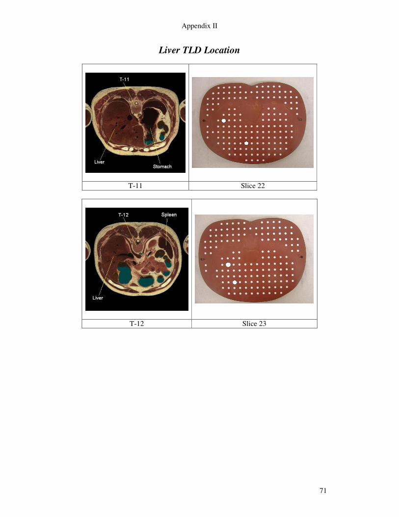
Appendix II

71

Liver TLD Location

T-11 Slice 22

T-12 Slice 23

Appendix II

72

Lung TLD Location

Slices 14 Slice 16

Slice 18

Appendix II

73

Bladder TLD Location

Human Slice Server Image Slice 32

Superimposed Imaged

Appendix II

74

Thyroid TLD Location

C-7 Slice 10

Appendix II

75

Colon TLD Location

Human Slice Server L1 Slice 26

Superimposed Imaged

L5 Slice 29

Appendix II

76

Oesophagus TLD Location

T-4 Slice 15

T-6 Slice 17

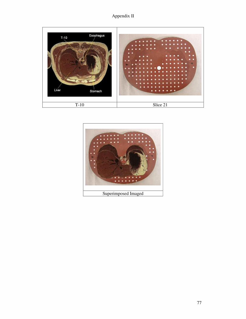
Appendix II

77

T-10 Slice 21

Superimposed Imaged

Appendix II

78

Brain TLD Location

Slice 3

Appendix II

79

Kidneys TLD Location

Slice 26

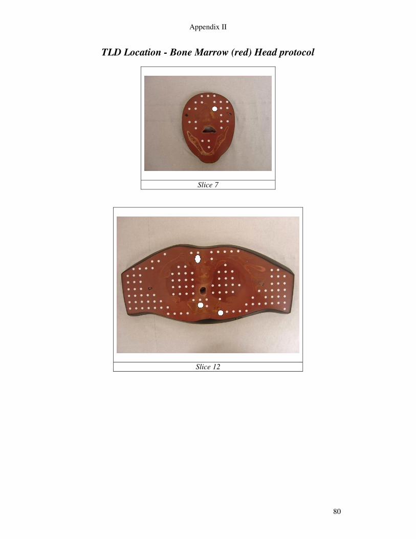
Appendix II

80

TLD Location - Bone Marrow (red) Head protocol

Slice 7

Slice 12

Appendix II

81

TLD Location - Bone Marrow (red) Chest protocol

Slice 14

Slice 18

Appendix II

82

TLD Location - Bone Marrow (red) Abdomen/Pelvis Protocol

Slice 23

Slice 25

Slice 29

Appendix II

83

5 References 1 P Dawson, Patient dose in MSCT: why is it increasing and does it matter? Br J Radiol. 2004;77:S10-S13 2 Shrimpton PC, Edyvean S., CT scanner dosimetry. Br J Radiol. 1998;71:1-3 3 Prokop M, General Principles of MDCT. European Journal of Radiology 2003;44:S4-S10 4 J G CAHIR, Multislice CT of the abdomen. Br J Radiol. 2004;77:S64–S73 5 Siemens AG, Medical Solutions (www.siemens.com/medical) Siemens Sensation 64. 6 Seeran, Computed Tomography. BC Canada: W.B. Saunders Company 2nd Edition, 2001:263 7 Claire McCann and Hamideh Alasti, Comparative evaluation of image quality from three CT simulation scanners. Journal of Applied Clinical Medical Physics 2004;Vol 5, No4 8 Conall J Garvey, Computed Tomography in clinical practise. BMJ 2002;324:1077-1080 9 Maria Lewis, Radiation dose issues in multi-slice CT scanning ImPACT technology update no.3 January 2005 10 Shrimpton PC, Edyvean S., CT scanner dosimetry. Br J Radiol. 1998;71:1-3 11 Hans Dieter Nagel PhD, Current Exposure Practice with Multislice CT. www.multislice-ct.com 12 S J Golding and P C Shrimpton, Radiation Dose in CT: Are we meeting the challenge? Br J Radiol 2002;74:1-4 13 Scheck R J, Radiation dose and image quality in spiral computed tomography: multi-centre evaluation at six institutions. Br J Radiol. 1998;71:734-744 14 G. Brix, H. D. Nagel, Radiation exposure in multi-slice versus single-slice spiral CT: results of a nationwide survey Eur Radiol 2003 13:1979–1991 15 P C Shrimpton et al Doses from Computed Tomography (CT) Examinations in the UK - 2003 Review (NRPB) 16 J G Van Unnik. Survey of CT techniques and absorbed dose in various Dutch hospitals. Br J Radiol. 1997;70:367-371

Appendix II

84

17 ICRP 60. 1990 Recommendations of the International Commission of Radiological Protection (publication 60). Oxford: Pergamon Press, 1991 18 RF Farr, Phyics for Medical Imaging W.B. Saunders Company Ltd 2000 19 DeWerd, L. A., Wagner, L. K. Characteristics of Radiation Detectors for Diagnostic Radiology. Appl. Radiat. Isot. 50, 125-136 (1999). 20 QADOS Berkshire, UK., http://www.qados.co.uk/thermo_harshaw_accessories.htm 21 European Commission (1999) Report EUR 16262 EN: European guidelines on quality criteria for computed tomography 22 McLean Donald, Survey of effective dose levels from typical paediatric CT protocols. Australsaian Radiology 2003; 47:135-142 23Seeran, Computed Tomography. BC Canada: W.B. Saunders Company 2nd Edition, 2001:263 24 Groves A M, 16-detector multislice CT: dosimetry estimation by TLD measurement compared with Monte Carlo simulation. Br J Radiol. 2004;77:662-665 25 European Commission (1999) Report EUR 16262 EN: European guidelines on quality criteria for computed tomography 26http://www.msct.info/CT_Quality_Criteria.htm#Download%20the%202004%20CT%20Quality%20Criteria 27 QADOS. Materials and Assemblies for Thermoluminescence Dosimetry. Harshaw TLD Thermoluminescence Dosimetry, QADOS. Berkshire, UK. 28 Fung, K. K. L. Investigation of dosimetric characteristics of the high sensitivity LiF:Mg,Cu,P Thermoluminescent Dosemeter and its applications in diagnostic radiology - a Review. Radiography. 10, 145-150 (2004). 29 Yipeng Li, B.S. ABSORBED DOSE MEASUREMENTS AND MCNP MODELING FOR THE LEKSELL GAMMA KNIFE 30 Model 3500 Manual TLD Reader with WinREMS Operator’s Manual. Publication No. 3500-W-O-0602-004. June 26, 2002 31 Dong, S. L., Chu, T. C., Lan, G.Y. et al. Characterization of high-sensitivity metal oxide semiconductor field effect transistor dosimeters system and LiF:Mg,Cu,P thermoluminescence dosimeters for use in diagnostic radiology. Appl. Radiat. Isot. 57, 883-891, (2002). 32 The Phantom Laboratory, Churchin Associated Ltd.

Appendix II

85

33 ICRP 60. 1990 Recommendations of the International Commission of Radiological Protection (publication 60). Oxford: Pergamon Press, 1991 34 M LAW, PhD et al. Patient effective dose from sentinel lymph node lymphoscintigraphy in breast cancer: a study using a female humanoid phantom and thermoluminescent dosimeters. The British Journal of Radiology, 76 (2003), 818–823 35 A M GROVES et al. 16-detector multislice CT: dosimetry estimation by TLD measurement compared with Monte Carlo simulation. The British Journal of Radiology, 77 (2004), 662–665 36 ImageJ developed at the National Institutes of Health. http://rsb.info.nih.gov/ij/ 37 Visible Human Server at the EPFL (Ecole Polytechnique Fédérale de Lausanne) http://visiblehuman.epfl.ch/index.php 38 Human Cross –Sectional Anatomy, Pocket Atlas of body sections and CT images. Harold Ellis, Bari Logan, Adrian Dixon. Butterworth-heinemann Ltd. (1994) 39 www.sirinet.net/~jgjohnso/skeleton.html (last accessed Sep 2005 ) 40 M. COHNEN et al. Radiation Exposure in Multi-Slice CT of the Heart. Fortschr Rontgenstr 2001; 173: 295-299 41 http://www.msct.info/CT_Quality_Criteria.htm#Download%20the%202004%20CT%20Quality%20Criteria 42 Peter Hunold, MD et al. Radiation Exposure during Cardiac CT: Effective Doses at Multi–Detector Row CT and Electron-Beam CT. Radiology 2003; 226:145–152 43 Estimating the effective dose to children undergoing heart investigations – a phantom study The British Journal of Radiology, 72 (1999), 378–383 44 S J YATES et al Effect of multislice scanners on patient dose from routine CT examinations in East Anglia, 2002. The British Journal of Radiology, 77 (2004), 472–478 45 Shrimpton et al, Doses from Computed Tomography examinations in the UK- 2003 Review 46 E G A AIRD, Second cancer risk, concomitant exposures and IRMER(2000)

assessment of effective dose in computed tomography …homepage.eircom.net/~gabbo1/documents/thesis...

Documents