assessment of discrimination of mafic rocks using …
TRANSCRIPT
ASSESSMENT OF DISCRIMINATION OF MAFIC ROCKS USING TRACE
ELEMENT SYSTEMATICS WITH MACHINE LEARNING
A THESIS SUBMITTED TO
THE GRADUATE SCHOOL OF NATURAL AND APPLIED SCIENCES
OF
MIDDLE EAST TECHNICAL UNIVERSITY
BY
MEHMET SINAN ÖZTÜRK
IN PARTIAL FULFILLMENT OF THE REQUIREMENTS
FOR
THE DEGREE OF DOCTOR OF PHILOSOPHY
IN
GEOLOGICAL ENGINEERING
DECEMBER 2019


Approval of the thesis:
ASSESSMENT OF DISCRIMINATION OF MAFIC ROCKS USING TRACE
ELEMENT SYSTEMATICS WITH MACHINE LEARNING
submitted by MEHMET SINAN ÖZTÜRK in partial fulfillment of the requirements
for the degree of Doctor of Philosophy in Geological Engineering Department,
Middle East Technical University by,
Prof. Dr. Halil Kalıpçılar
Dean, Graduate School of Natural and Applied Sciences
Prof. Dr. Erdin Bozkurt
Head of Department, Geological Engineering
Assoc. Prof. Dr. Kaan Sayıt
Supervisor, Geological Engineering, METU
Examining Committee Members:
Assoc. Prof. Dr. Biltan Kürkçüoğlu
Geological Engineering, Hacettepe University
Assoc. Prof. Dr. Kaan Sayıt
Geological Engineering, METU
Assist. Prof. Dr. Fatma Toksoy Köksal
Geological Engineering, METU
Assist. Prof. Dr. Ali İmer
Geological Engineering, METU
Assoc. Prof. Dr. H. Evren Çubukçu
Geological Engineering, Hacettepe University
Date: 27.12.2019

iv
I hereby declare that all information in this document has been obtained and
presented in accordance with academic rules and ethical conduct. I also declare
that, as required by these rules and conduct, I have fully cited and referenced all
material and results that are not original to this work.
Name, Surname:
Signature:
Mehmet Sinan Öztürk
v
ABSTRACT
ASSESSMENT OF DISCRIMINATION OF MAFIC ROCKS USING TRACE
ELEMENT SYSTEMATICS WITH MACHINE LEARNING
Öztürk, Mehmet Sinan
Doctor of Philosophy, Geological Engineering
Supervisor: Assoc. Prof. Dr. Kaan Sayıt
December 2019, 294 pages
Having an important role in the elucidation of the evolution of ancient oceans and
related continental fragments, the determination of original tectonic settings of ancient
igneous rocks is an essential part of the geodynamic inferences. Geochemical
classification of mafic rocks is important for the tectono-magmatic discrimination of
igneous rocks especially when geological information is insufficient as the link of the
igneous rocks to their original tectonic setting had been erased due to large scale
events.
Starting from 1960s, first traditional methods (functions of elements or element ratios,
bivariate and ternary diagrams of elements or element ratios), and then, recently,
modern methods such as decision trees, support vector machines, sparse multinomial
regression and random forest have been applied to develop tectono-magmatic
discrimination methods.
The purpose of this study is to assess new and better classification methods which are
both statistically and geochemically rigorous using trace element systematics with
decision tree learning, an effective machine learning method for classification. Dataset
included a large number of samples well distributed through different tectonic settings
(continental arcs, continental within-plates, mid-oceanic ridges, oceanic arcs, oceanic

vi
back-arc basins, oceanic islands and oceanic plateaus) as classes. Data is gathered
from high quality articles which is known to follow accurate geochemical sampling
procedures and have their samples analyzed in internationally accredited and
trustworthy laboratories. Only element ratios have been used as features in order to
increase the successful applicability of constructed decision trees to external datasets.
With this study, successful decision trees with their alternatives are proposed for the
tectono-magmatic discrimination between (1) subduction and non-subduction
settings, (2) arc-related and back-arc-related settings within subduction settings, (3)
oceanic arcs and continental arcs within arc-related settings, (4) oceanic and
continental settings within subduction settings, (5) oceanic arcs and oceanic back-arcs
within subduction-related oceanic settings, (6) mid-oceanic ridges + oceanic plateaus
and oceanic islands + continental within-plates within non-subduction settings, (7)
mid-oceanic ridges and oceanic plateaus within non-subduction settings and (8)
oceanic islands and continental within-plates within non-subduction settings.
Keywords: Decision trees, machine learning, tectonic discrimination, mafic rocks,
trace elements
vii
ÖZ
MAFİK KAYAÇLARIN AYIRDIMLANMASININ ESER ELEMENT
SİSTEMATİĞİ KULLANILARAK MAKİNE ÖĞRENİMİ İLE
DEĞERLENDİRİLMESİ
Öztürk, Mehmet Sinan
Doktora, Jeoloji Mühendisliği
Tez Danışmanı: Doç. Dr. Kaan Sayıt
Aralık 2019, 294 sayfa
Eski magmatik kayaçların original tektonik ortamlarının belirlenmesi, eski
okyanusların ve ilgili kıta parçalarının evriminin aydınlatılmasında önemli bir rol
oynamakla birlikte; jeodinamik çıkarımların yapılması açısından önemli bir konudur.
Mafik kayaçların jeokimyasal sınıflandırması, özellikle kayaç ile original tektonik
ortamı arasındaki bağlantının büyük ölçekli olayların etkisiyle silindiği ve yeterli
jeolojik bilginin mevcut olmadığı durumlarda, magmatik kayaçların tektono-
magmatik olarak ayırdımlanması için önemli hale gelmektedir.
1960’lı yıllardan başlayarak, tektono-magmatik ayırdımlama yöntemleri geliştirmek
amacıyla, önce geleneksel yöntemler (element veya element oranlarının kullanıldığı
fonksiyonlar, iki veya üç değişkenli diyagramlar) ve daha sonra ise, özellikle son
zamanlarda karar ağaçları, destek vektör makineleri, seyrek multinomial regresyon ve
rastgele orman gibi modern yöntemler kullanılmıştır.
Bu çalışmanın amacı, eser element sistematiği ile birlikte sınıflandırmalar için etkin
bir makine öğrenimi yöntemi olan karar ağacı öğrenmesini kullanarak hem istatistiksel
hem de jeokimyasal açıdan daha titiz, daha yeni ve daha iyi sınıflandırma yöntemleri
önermektir. Çalışmada kullanılan verisetinde, sınıflar olarak farklı tektonik ortamlara
(kıtasal yay, kıta içi tabakaları, okyanus ortası sırtları, oknayus yayları, okyanus yay
viii
arkası havzaları, okyanus adaları ve okyanus platoları) ait iyi dağılım gösteren çok
sayıda numune içermektedir. Veri, doğru jeokimyasal numuneleme prosedürleri takip
edilerek örneklenen ve uluslararası akreditasyona sahip güvenilir laboratuvarlarda
analiz edilmiş numunelerin kullanıldığı yüksek kaliteli makalelerden elde edilmiştir.
Sınıflandırmada, oluşturulan karar ağaçlarının harici very setlerine de başarıyla
uygulanabilmesi amacıyla, parameter olarak sadece element oranları kullanılmıştır.
Bu çalışma ile, (1) yitim zonlarında yer alan ve yer almayan tektonik ortamlar, (2)
yitim zonlarında, yay içerisinde veya yay gerisinde bulunan tektonik ortamlar, (3) yay
içerisinde yer alan okyanus yayları (OA) ve karasal yaylar (CA), (4) yitim zonlarında
okyanusal ortama ait ve karasal ortama ait tektonik ortamlar, (5) okyanusal ortama ait
yitim zonlarında yay içerisinde (OA) veya yay gerisinde (OBAB) yer alan tektonik
ortamlar, (6) yitim zonlarında yer almayan tektonik ortamlar arasında okyanus ortası
sırtı ve okyanus platosu (MOR ve OP) ile okyanus adası ve karasal kıta içi (OI ve
CWP), (7) okyanus ortası sırtı (MOR) ve okyanus platosu (OP) ile (8) okyanus adası
(OI) ve karasal kıta içi (CWP) tektonik ortamlarını birbirinden başarıyla ayırdımlamak
amacıyla alternatifleri ile birlikte, karar ağaçları oluşturulmuş ve önerilmiştir.
Anahtar Kelimeler: Karar ağaçları, makine öğrenimi, tektonik ayırdımlama, mafik
kayaçlar, eser elementler

ix
To my wife, Evrim Öztürk;

x
ACKNOWLEDGEMENTS
First, I would like to express my sincere gratitude to my advisor Assoc. Prof. Dr. Kaan
Sayıt for the continuous support for my Ph.D. study and related research, for his
patience, motivation and immense knowledge. His guidance helped me in all the time
of research and writing of this thesis. I could not have imagined having a better advisor
and mentor for my Ph.D. study.
Besides my advisor, I would like to thank to my thesis committee for their insightful
comments and valuable guidance through my Ph.D. study.
I would like to thank to my wife, Evrim Öztürk as she always supported me in all
means and encouraged me to finish my Ph.D. study. This study could not have been
finished at all without her continuous support, encouragement and patience.
Finally, I would like to thank to members of my family for their supports throughout
writing this thesis and my life in general, and my friend, Ayşe Peksezer Sayıt for
insightful comments and encouragement and also for the questions and advices which
incented me to widen my research from various perspectives.

xi
TABLE OF CONTENTS
ABSTRACT ................................................................................................................. v
ÖZ….. ....................................................................................................................... vii
ACKNOWLEDGEMENTS ......................................................................................... x
TABLE OF CONTENTS ........................................................................................... xi
LIST OF TABLES ................................................................................................... xvi
LIST OF FIGURES ................................................................................................. xxi
LIST OF ABBREVIATIONS ................................................................................ xxix
CHAPTERS
1. INTRODUCTION ................................................................................................ 1
1.1. Purpose and Scope ............................................................................................. 1
1.2. Review of Tectono-Magmatic Discrimination Methods of Basic Igneous Rocks
.................................................................................................................................. 8
1.2.1. Elements as Discriminating Criteria ........................................................... 9
1.2.2. Traditional Bivariate Diagrams ................................................................ 10
1.2.3. Traditional Ternary Diagrams .................................................................. 24
1.2.4. Traditional Diagrams with Discriminating Functions .............................. 30
1.2.5. New Multi-Dimensional Diagrams with Discriminating Functions ......... 35
1.2.6. Discrimination using Machine Learning Methods ................................... 39
2. DATABASE AND METHODOLOGY ............................................................. 45
2.1. Data Gathering and Import .............................................................................. 45
2.2. Data Cleaning .................................................................................................. 45
2.3. Classes (Tectonic Settings) ............................................................................. 47
xii
2.4. Feature Selection ............................................................................................. 50
2.5. Splitting Database ........................................................................................... 55
2.6. Methodology (Decision Tree Learning) ......................................................... 55
2.6.1. Non-Mathematical Explanation of Decision Tree Learning .................... 55
2.6.2. Mathematical Explanation of Decision Tree Learning ............................ 59
2.6.3. Evaluation of Decision Trees ................................................................... 63
2.6.3.1. Generalization Error and Classification Accuracy ............................ 63
2.6.3.2. Alternatives for Accuracy Measurement ........................................... 63
2.6.3.3. Confusion Matrix ............................................................................... 65
2.6.3.4. ROC Curve ........................................................................................ 66
2.6.3.5. Lift Curve ........................................................................................... 66
2.6.3.6. Area Under Curve (AUC) .................................................................. 67
2.6.4. Splitting Decision Trees ........................................................................... 68
2.6.4.1. Impurity-based criteria ....................................................................... 68
2.6.4.2. Information Gain ............................................................................... 68
2.6.4.3. Gini Index .......................................................................................... 69
2.6.4.4. Gain Ratio .......................................................................................... 69
2.6.5. Stopping Decision Trees .......................................................................... 69
2.6.6. Pruning Decision Trees ............................................................................ 70
2.6.7. Advantages and Disadvantages of Decision Trees ................................... 70
2.6.8. Application of Decision Tree Learning to Tectono-Magmatic
Discrimination .................................................................................................... 71
3. RESULTS ........................................................................................................... 77
3.1. Constructed Decision Trees ............................................................................ 77
xiii
3.1.1. Discrimination Between Subduction and Non-Subduction Settings ........ 77
3.1.2. Discrimination Within Subduction Settings ............................................. 80
3.1.2.1. The First Path for Discrimination Within Subduction Settings ......... 81
3.1.2.2. The Second Path for Discrimination Within Subduction Settings ..... 88
3.1.3. Discrimination Within Non-Subduction Settings ..................................... 97
3.1.3.1. Discrimination Between Group 1 (Mid-Oceanic Ridge and Oceanic
Plateau) and Group 2 (Oceanic Island and Continental Within-plate) Settings
......................................................................................................................... 97
3.1.3.2. Discrimination Between Mid-Oceanic Ridges and Oceanic Plateaus
....................................................................................................................... 102
3.1.3.3. Discrimination Between Oceanic Islands and Continental Within-
plates ............................................................................................................. 102
3.2. Classification Results (Decision Trees) ........................................................ 111
3.2.1. Discrimination Between Subduction and Non-Subduction Settings ...... 111
3.2.2. Discrimination Within Subduction Settings ........................................... 120
3.2.2.1. The First Path for Discrimination Within Subduction Settings ....... 120
3.2.2.2. The Second Path for Discrimination Within Subduction Settings ... 131
3.2.3. Discrimination Within Non-Subduction Settings ................................... 148
3.2.3.1. Discrimination Between Group 1 (Mid-Oceanic Ridge and Oceanic
Plateau) and Group 2 (Oceanic Island and Continental Within-plate) Settings
....................................................................................................................... 148
3.2.3.2. Discrimination Between Mid-Oceanic Ridges and Oceanic Plateaus
....................................................................................................................... 157
3.2.3.3. Discrimination Between Oceanic Islands and Continental Within-
plates ............................................................................................................. 163
4. DISCUSSION ................................................................................................... 171

xiv
4.1. Discussion of Decision Trees ........................................................................ 171
4.1.1. Discussion Based on Information Gain .................................................. 171
4.1.2. Discussion Based on Lift Curves and ROC Curves ............................... 179
4.1.3. Discussion Based on Statistical Evaluation of Decision Trees .............. 179
4.2. Discussion of Classification Results ............................................................. 184
4.2.1. Discrimination Between Subduction and Non-Subduction Settings ...... 184
4.2.2. Discrimination Within Subduction Settings ........................................... 195
4.2.2.1. The First Path for Discrimination Within Subduction Settings ....... 195
4.2.2.2. The Second Path for Discrimination Within Subduction Settings .. 207
4.2.3. Discrimination Within Non-Subduction Settings ................................... 218
4.2.3.1. Discrimination Between Group 1 (Mid-Oceanic Ridge and Oceanic
Plateau) and Group 2 (Oceanic Island and Continental Within-plate) Settings
...................................................................................................................... 218
4.2.3.2. Discrimination Between Mid-Oceanic Ridges and Oceanic Plateaus
...................................................................................................................... 224
4.2.3.3. Discrimination Between Oceanic Islands and Continental Within-
plates ............................................................................................................. 229
4.3. Comparison with Traditional Discrimination Methods ................................ 232
4.3.1. Wood (1980) for Discrimination Between Subduction and Non-Subduction
Settings ............................................................................................................. 233
4.3.2. Pearce and Peate (1995) for Discrimination Between Subduction and Non-
Subduction Settings .......................................................................................... 235
4.3.3. Saccani (2015) for Discrimination Between Subduction and Non-
Subduction Settings and Within Subduction Settings ...................................... 236
4.4. Recommended Decision Trees for Discriminations ..................................... 239

xv
4.4.1. Recommended Decision Trees for Discrimination between Subduction and
Non-Subduction ................................................................................................ 239
4.4.2. Recommended Decision Trees for Discrimination between Arc and Back-
arc ..................................................................................................................... 240
4.4.3. Recommended Decision Trees for Discrimination between Oceanic Arc
and Continental Arc .......................................................................................... 242
4.4.4. Recommended Decision Trees for Discrimination between Oceanic and
Continental Settings .......................................................................................... 242
4.4.5. Recommended Decision Trees for Discrimination between Oceanic Arc
and Back-arc ..................................................................................................... 247
4.4.6. Recommended Decision Trees for Discrimination between Group 1 and
Group 2 of Non-Subduction Settings ............................................................... 247
4.4.7. Recommended Decision Trees for Discrimination between Mid-Ocean
Ridges and Oceanic Plateaus ............................................................................ 247
4.4.8. Recommended Decision Trees for Discrimination between Oceanic Islands
and Continental Within-Plates .......................................................................... 252
5. CONCLUSIONS .............................................................................................. 255
REFERENCES ......................................................................................................... 259
CURRICULUM VITAE .......................................................................................... 293
xvi
LIST OF TABLES
TABLES
Table 1.1. Discrimination functions used in diagrams of Pearce (1976) ................... 31
Table 1.2. Discrimination functions used in diagrams of Butler and Woronow (1986)
................................................................................................................................... 32
Table 1.3. Discrimination functions used in diagrams of Velikoslavinsky and
Kykrylov (2014) ........................................................................................................ 35
Table 1.4. Discrimination functions used in diagrams of Agrawal et al. (2004) ....... 36
Table 1.5. Discrimination functions used in diagrams of Verma et al. (2006) .......... 37
Table 1.6. Discrimination functions used in diagrams of Verma et al. (2006) .......... 39
Table 2.1. Brief Information on Tectonic Settings .................................................... 49
Table 2.2. Structure of a confusion matrix ................................................................ 65
Table 2.3. Information gain, gain ratio and gini index of most discriminative features
................................................................................................................................... 74
Table 3.1 Subduction settings .................................................................................... 80
Table 3.2. Confusion Matrix Summary for Training and Test Datasets for Tectono-
Magmatic Discrimination Between Subduction and Non-Subduction Settings ...... 113
Table 3.3. Confusion Matrix Summary for External Datasets for Tectono-Magmatic
Discrimination Between Subduction and Non-Subduction Settings ....................... 114
Table 3.4. Misclassifications in training and test datasets by decision trump for
discrimination between subduction and non-subduction settings ........................... 114
Table 3.5. Misclassifications in external datasets by decision stump for discrimination
between subduction and non-subduction settings .................................................... 115
Table 3.6. Misclassifications in training and test datasets by first decision tree for
discrimination between subduction and non-subduction settings ........................... 116
Table 3.7. Misclassifications in external datasets by first decision tree for
discrimination between subduction and nonsubduction settings ............................. 117
xvii
Table 3.8. Misclassifications in training and test datasets by second decision tree for
discrimination between subduction and non-subduction settings ............................ 118
Table 3.9. Misclassifications in external datasets by second decision tree for
discrimination between subduction and non-subduction settings ............................ 119
Table 3.10. Confusion Matrix Summary for Training and Test Datasets for Tectono-
Magmatic Discrimination Between Arc and Back-arc-related Settings .................. 123
Table 3.11. Confusion Matrix Summary for External Datasets for Tectono-Magmatic
Discrimination Between Arc and Back-arc-related Settings ................................... 123
Table 3.12. Misclassifications by first decision tree for discrimination between arc and
back-arc settings ....................................................................................................... 124
Table 3.13. Misclassifications by first decision tree for discrimination between arc and
back-arc settings ....................................................................................................... 125
Table 3.14. Misclassifications by second decision tree for discrimination between arc
and back-arc settings ................................................................................................ 126
Table 3.15. Misclassifications by second decision tree for discrimination between arc
and back-arc settings ................................................................................................ 127
Table 3.16. Confusion Matrix Summary for Training and Test Datasets for Tectono-
Magmatic Discrimination Between Oceanic Arc and Continental Arc Settings ..... 130
Table 3.17. Confusion Matrix Summary for External Dataset for Tectono-Magmatic
Discrimination Between Oceanic Arc and Continental Arc Settings ...................... 131
Table 3.18. Misclassifications by first decision tree for discrimination between
oceanic arc and continental-arc settings ................................................................... 132
Table 3.19. Misclassifications by first decision tree for discrimination between
oceanic arc and continental-arc settings ................................................................... 133
Table 3.20. Misclassifications by second decision tree for discrimination between
oceanic arc and continental-arc settings ................................................................... 134
Table 3.21. Misclassifications by second decision tree for discrimination between
oceanic arc and continental-arc settings ................................................................... 135
Table 3.22. Confusion Matrix Summary for Training and Test Datasets for Tectono-
Magmatic Discrimination Between Oceanic and Continental Settings ................... 138
xviii
Table 3.23. Confusion Matrix Summary for External Dataset for Tectono-Magmatic
Discrimination Between Oceanic and Continental Related Settings ....................... 138
Table 3.24. Misclassifications by first decision tree for discrimination between
oceanic and continental settings .............................................................................. 139
Table 3.25. Misclassifications by first decision tree for discrimination between
oceanic and continental settings .............................................................................. 140
Table 3.26. Misclassifications by second decision tree for discrimination between
oceanic and continental settings .............................................................................. 141
Table 3.27. Misclassifications by second decision tree for discrimination between
oceanic and continental settings .............................................................................. 142
Table 3.28. Confusion Matrix Summary for Training and Test Datasets for Tectono-
Magmatic Discrimination Between Oceanic Arc and Oceanic Back-Arc Settings . 146
Table 3.29. Confusion Matrix Summary for External Dataset for Tectono-Magmatic
Discrimination Between Oceanic Arc and Oceanic Back-Arc Settings .................. 146
Table 3.30. Misclassifications by first decision tree for discrimination between
oceanic arc and oceanic back-arc settings ............................................................... 146
Table 3.31. Misclassifications by first decision tree for discrimination between
oceanic arc and oceanic back-arc settings ............................................................... 147
Table 3.32. Misclassifications by second decision tree for discrimination between
oceanic arc and oceanic back-arc settings ............................................................... 147
Table 3.33. Misclassifications by second decision tree for discrimination between
oceanic arc and oceanic back-arc settings ............................................................... 148
Table 3.34. Confusion Matrix Summary for Training and Test Datasets for Tectono-
Magmatic Discrimination Between Group 1 and Group 2 of Non-Subduction Settings
................................................................................................................................. 151
Table 3.35. Confusion Matrix Summary for External Dataset for Tectono-Magmatic
Discrimination Between Group 1 and Group 2 of Non-Subduction Settings ......... 152
Table 3.36. Misclassifications by first decision tree for discrimination between group
1 and group 2 of non-subduction settings ................................................................ 153
xix
Table 3.37. Misclassifications by first decision tree for discrimination between group
1 and group 2 of non-subduction settings ................................................................ 154
Table 3.38. Misclassifications by second decision tree for discrimination between
group 1 and group 2 of non-subduction settings ...................................................... 155
Table 3.39. Misclassifications by second decision tree for discrimination between
group 1 and group 2 of non-subduction settings ...................................................... 156
Table 3.40. Confusion Matrix Summary for Training and Test Datasets for Tectono-
Magmatic Discrimination Between Mid-Oceanic Ridge and Oceanic Plateau Settings
.................................................................................................................................. 160
Table 3.41. Confusion Matrix Summary for External Dataset for Tectono-Magmatic
Discrimination Between Mid-Oceanic Ridge and Oceanic Plateaus ....................... 160
Table 3.42. Misclassifications by first decision tree for discrimination between mid-
oceanic ridge and oceanic plateaus .......................................................................... 161
Table 3.43. Misclassifications by first decision tree for discrimination between mid-
oceanic ridge and oceanic plateaus .......................................................................... 161
Table 3.44. Misclassifications by second decision tree for discrimination between
mid-oceanic ridge and oceanic plateaus ................................................................... 162
Table 3.45. Misclassifications by second decision tree for discrimination between
mid-oceanic ridge and oceanic plateaus ................................................................... 162
Table 3.46. Confusion Matrix Summary for Training and Test Datasets for Tectono-
Magmatic Discrimination Between Ocean Islands and Continental Within-plates . 166
Table 3.47. Confusion Matrix Summary for External Dataset for Tectono-Magmatic
Discrimination Between Oceanic Islands and Continental Within-plates ............... 166
Table 3.48. Misclassifications by first decision tree for discrimination between
oceanic islands and continental within-plates .......................................................... 167
Table 3.49. Misclassifications by first decision tree for discrimination between
oceanic islands and continental within-plates .......................................................... 168
Table 3.50. Misclassifications by second decision tree for discrimination between
oceanic islands and continental within-plates .......................................................... 169

xx
Table 3.51. Misclassifications by second decision tree for discrimination between
oceanic islands and continental within-plates .......................................................... 170
Table 4.1. Information gain values of selected features for tectono-magmatic
discriminations ......................................................................................................... 172
Table 4.2. Statistical considerations for discrimination between subduction and non-
subduction settings ................................................................................................... 182
Table 4.3. Statistical considerations for discrimination between arc and back-arc
settings ..................................................................................................................... 182
Table 4.4. Statistical considerations for discrimination between oceanic and
continental arcs ........................................................................................................ 182
Table 4.5. Statistical considerations for discrimination between oceanic and
continental settings .................................................................................................. 183
Table 4.6. Statistical considerations for discrimination between Oceanic Arc and
Oceanic Back-Arc Basins ........................................................................................ 183
Table 4.7. Statistical considerations for discrimination between Group 1 and Group 2
of Non-Subduction Settings ..................................................................................... 183
Table 4.8. Statistical considerations for discrimination between Mid-Ocean Ridge and
Oceanic Plateau ....................................................................................................... 184
Table 4.9. Statistical considerations for discrimination between Ocean Island and
Continental Within-Plate ......................................................................................... 184

xxi
LIST OF FIGURES
FIGURES
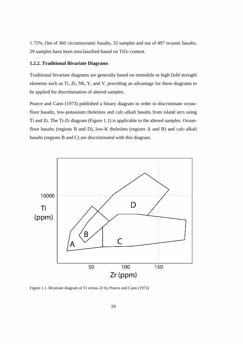
Figure 1.1. Bivariate diagram of Ti versus Zr by Pearce and Cann (1973) ............... 10
Figure 1.2. Bivariate diagram of Ti versus Zr by Dilek and Furnes (2009) .............. 11
Figure 1.3. Bivariate diagram of Pearce (1975) ......................................................... 12
Figure 1.4. Bivariate diagram of Pearce and Gale (1977) .......................................... 14
Figure 1.5. Bivariate diagram of Pearce and Norry (1979) ........................................ 14
Figure 1.6. Bivariate diagram of Pearce et al. (1981) ................................................ 15
Figure 1.7. Bivariate diagrams of Peace (1982) using Ti/Y versus Nb/Y ................. 16
Figure 1.8. Bivariate diagrams of Peace (1982) using K2O/Yb versus Ta/Yb .......... 16
Figure 1.9. Bivariate diagrams of Peace (1982) using Ce/Yb versus Ta/Yb ............. 17
Figure 1.10. Bivariate diagram of Shervais (1982) .................................................... 18
Figure 1.11. Bivariate diagrams by Pearce (1983) using Ta/Yb versus Th/Nb ......... 19
Figure 1.12. Bivariate diagrams by Pearce (1983) using Zr versus Zr/Y .................. 19
Figure 1.13. Bivariate diagram of TiO2 versus Cr by Pearce et al. (1984) ................ 20
Figure 1.14. Bivariate diagram of Y versus Cr by Dilek et al. (2007) ....................... 21
Figure 1.15. Bivariate diagrams of Hollocher (2012) using La/Yb vs Nb/La ........... 22
Figure 1.16. Bivariate diagrams of Hollocher (2012) using La/Yb vs Th/Nb ........... 22
Figure 1.17. Bivariate diagrams of Saccani (2015) using normalized values of Th
versus Nb .................................................................................................................... 23
Figure 1.18. Discrimination diagrams of Pearce and Cann (1973) using Ti/100-Zr-Y*3
.................................................................................................................................... 25
Figure 1.19. Discrimination diagrams of Pearce and Cann (1973) using Ti/100-Zr-Sr/2
.................................................................................................................................... 26
Figure 1.20. Discrimination diagram of Wood (1980), modified after Wood et al.
(1979) using Hf/3, Th and Nb/16 ............................................................................... 27
xxii
Figure 1.21. Discrimination diagram of Mullen (1983) using TiO2, MnO*10, P2O5*10
................................................................................................................................... 28
Figure 1.22. Discrimination diagram of Meschede (1986) using 2*Nb, Zr/4 and Y 29
Figure 1.23. Discrimination diagram of Cabanis and Lecolle (1989) using Y/15, La/10
and Nb/8 ..................................................................................................................... 30
Figure 1.24. Discrimination diagrams of Pearce (1976) using DF1 and DF2 ........... 31
Figure 1.25. Discrimination diagrams of Pearce (1976) using DF2 and DF3 ........... 32
Figure 1.26. Discrimination diagrams of Pearce (1976) using DF1 and DF2 ........... 33
Figure 1.27. Discrimination diagrams of Velikoslavinsky and Kykrylov (2014) using
discrimination functions of (A) by major element contents, (B) by inert minor element
contents ...................................................................................................................... 34
Figure 1.28. Representative discrimination diagram from Agrawal et al. (2004) ..... 36
Figure 1.29. Representative discrimination diagram from Verma et al. (2006) ........ 37
Figure 1.30. Representative discrimination diagram from Agrawal et al. (2008) ..... 38
Figure 1.31. Representative discrimination diagrams from Verma and Agrawal et al.
(2011) ......................................................................................................................... 40
Figure 1.32. Decision tree from Vermeesch (2006a) using all elements ................... 41
Figure 1.33. Decision tree from Vermeesch (2006a) using only relatively immobile
elements ..................................................................................................................... 42
Figure 2.1. The difference between the discrimination potential of element ratios and
their absolute abundance ............................................................................................ 53
Figure 2.2. Representative example to strong correlation between selected relatively
immobile elements and elements eliminated due to high amount of missing data ... 54
Figure 2.3. Structure of a decision tree ...................................................................... 56
Figure 2.4. Underfitting and overfitting examples .................................................... 58
Figure 2.5. Representation of optimum model based on prediction errors on training
and external datasets .................................................................................................. 59
Figure 2.6. Representation of a decision tree in a two-dimensional graph ................ 61
Figure 2.7. Graph of recall versus precision .............................................................. 64
xxiii
Figure 2.8. Representation of false positive (FP), true positive (TP) and false negative
(FN) ............................................................................................................................ 64
Figure 2.9. Graph of true positive rate versus false positive rate ............................... 66
Figure 2.10. Lift curve graph ..................................................................................... 67
Figure 2.11. Graph of true positive versus false positive ........................................... 67
Figure 2.12. Flowchart for the tectono-magmatic discrimination of rocks................ 73
Figure 3.1. Decision stump for discrimination between subduction and non-
subduction settings ..................................................................................................... 78
Figure 3.2. The first decision tree to discriminate between subduction and non-
subduction settings ..................................................................................................... 78
Figure 3.3. The second decision tree to discriminate between subduction and non-
subduction settings ..................................................................................................... 79
Figure 3.4. Decision rule for the decision stump ....................................................... 79
Figure 3.5. Decision rule for the first decision tree.................................................... 79
Figure 3.6. Decision rule for the second decision tree ............................................... 80
Figure 3.7. The first decision tree to discriminate between arc and back-arc-related
settings ....................................................................................................................... 81
Figure 3.8. The second decision tree to discriminate between arc and back-arc-related
settings ....................................................................................................................... 82
Figure 3.9. Decision rule for the first decision tree.................................................... 82
Figure 3.10. Decision rule for the second decision tree ............................................. 83
Figure 3.11. The first decision tree to discriminate within arc-related settings ......... 84
Figure 3.12. The second decision tree to discriminate within arc-related settings .... 85
Figure 3.13. Decision rule for the first decision tree.................................................. 86
Figure 3.14. Decision rule for the second decision tree ............................................. 87
Figure 3.15. The first decision tree to discriminate between oceanic and continental
settings ....................................................................................................................... 89
Figure 3.16. The second decision tree to discriminate between oceanic and continental
settings ....................................................................................................................... 90
Figure 3.17. Decision rule for the first decision tree.................................................. 91
xxiv
Figure 3.18. Decision rule for the second decision tree ............................................ 92
Figure 3.19. The first decision tree to discriminate within oceanic settings ............. 93
Figure 3.20. The second decision tree to discriminate within oceanic settings ......... 94
Figure 3.21. Decision rule for the first decision tree ................................................. 95
Figure 3.22. Decision rule for the second decision tree ............................................ 96
Figure 3.23. The first decision tree to discriminate within non-subduction settings . 98
Figure 3.24. The second decision tree to discriminate within non-subduction settings
................................................................................................................................... 99
Figure 3.25. Decision rule for the first decision tree ............................................... 100
Figure 3.26. Decision rule for the second decision tree .......................................... 101
Figure 3.27. The first decision tree to discriminate between Mid-Oceanic Ridges and
Oceanic Plateaus ...................................................................................................... 103
Figure 3.28. The second decision tree to discriminate between Mid-Oceanic Ridges
and Oceanic Plateaus ............................................................................................... 104
Figure 3.29. Decision rule for the first decision tree ............................................... 105
Figure 3.30. Decision rule for the second decision tree .......................................... 106
Figure 3.31. The first decision tree to discriminate between Ocean Islands and
Continental Within-Plates ........................................................................................ 107
Figure 3.32. The second decision tree to discriminate between Ocean Islands and
Continental Within-Plates ........................................................................................ 108
Figure 3.33. Decision rule for the first decision tree ............................................... 109
Figure 3.34. Decision rule for the second decision tree .......................................... 110
Figure 3.35. Classification results of the decision stump to discriminate between
subduction and non-subduction settings .................................................................. 111
Figure 3.36. Classification results of the first decision tree to discriminate between
subduction and non-subduction settings .................................................................. 112
Figure 3.37. Classification results of the second decision tree to discriminate between
subduction and non-subduction settings .................................................................. 113
Figure 3.38. Classification results of the first decision tree to discriminate between arc
and back-arc-related settings ................................................................................... 121

xxv
Figure 3.39. Classification results of the second decision tree to discriminate between
arc and back-arc-related settings .............................................................................. 122
Figure 3.40. Classification results of the first decision tree to discriminate within arc-
related settings .......................................................................................................... 128
Figure 3.41. Classification results of the second decision tree to discriminate within
arc-related settings ................................................................................................... 129
Figure 3.42. Classification results of the first decision tree to discriminate between
oceanic and continental settings ............................................................................... 136
Figure 3.43. Classification results of the second decision tree to discriminate between
oceanic and continental settings ............................................................................... 137
Figure 3.44. Classification results of the first decision tree to discriminate within
oceanic settings ........................................................................................................ 144
Figure 3.45. Classification results of the second decision tree to discriminate within
oceanic settings ........................................................................................................ 145
Figure 3.46. Classification results of the first decision tree to discriminate between
mid-oceanic ridge + oceanic plateau and oceanic island + continental-within plates
.................................................................................................................................. 149
Figure 3.47. Classification results of the second decision tree to discriminate between
mid-oceanic ridge + oceanic plateau and oceanic island + continental-within plates
.................................................................................................................................. 150
Figure 3.48. Classification results of the second decision tree to discriminate between
mid-oceanic ridge + oceanic plateau and oceanic island + continental-within plates
.................................................................................................................................. 150
Figure 3.49. Classification results of the first decision tree to discriminate between
mid-oceanic ridge and oceanic plateaus ................................................................... 158
Figure 3.50. Classification results of the second decision tree to discriminate between
mid-oceanic ridge and oceanic plateaus ................................................................... 159
Figure 3.51. Classification results of the first decision tree to discriminate between
oceanic island and continental-within plates ............................................................ 164
xxvi
Figure 3.52. Classification results of the second decision tree to discriminate between
oceanic island and continental-within plates ........................................................... 165
Figure 4.1. Comparison of spider-diagrams between samples from continental within-
plates misclassified as oceanic island and samples of oceanic islands correctly
classified (normalization coefficients are based on Sun and McDonough, 1995) .. 177
Figure 4.2. Comparison of spider-diagrams between samples oceanic islands
misclassified as continental within-plate and samples of continental within-plate
correctly classified (normalization coefficients are based on Sun and McDonough,
1995) ........................................................................................................................ 178
Figure 4.3. Lift curve for tectonic discriminations .................................................. 180
Figure 4.4. ROC for tectonic discriminations .......................................................... 181
Figure 4.5. Comparison of spider-diagrams between samples continental within-plates
and subduction-related settings (normalization coefficients are based on Sun and
McDonough, 1995) .................................................................................................. 193
Figure 4.6. Comparison of spider-diagrams between samples from OBAB
misclassified as MOR and samples from MOR (normalization coefficients are based
on Sun and McDonough, 1995) ............................................................................... 194
Figure 4.7. Comparison of spider-diagrams between samples from oceanic plateaus
misclassified as mid-ocean ridges and samples of mid-ocean ridges correctly classified
(normalization coefficients are based on Sun and McDonough, 1995) ................... 228
Figure 4.8. Samples of subduction settings plotted on Wood (1980) diagram ........ 233
Figure 4.9. Samples of non-subduction settings plotted on Wood (1980) diagram 234
Figure 4.10. Samples of subduction settings plotted on Pearce and Peate (1995)
diagram .................................................................................................................... 235
Figure 4.11. Samples of non-subduction settings plotted on Pearce and Peate (1995)
diagram .................................................................................................................... 236
Figure 4.12. Samples of subduction settings plotted on Saccani (2015) diagram ... 237
Figure 4.13. Samples of non-subduction settings plotted on Saccani (2015) diagram
................................................................................................................................. 237
Figure 4.14. Samples of arc settings plotted on Saccani (2015) diagram ................ 238

xxvii
Figure 4.15. Samples of back-arc settings plotted on Saccani (2015) diagram ....... 239
Figure 4.16. Recommended simplified version of the first decision tree for the
discrimination between subduction and non-subduction ......................................... 240
Figure 4.17. Recommended simplified version of the first decision tree for the
discrimination between arc and back-arc settings .................................................... 241
Figure 4.18. Recommended simplified version of the alternative decision tree for the
discrimination between arc and back-arc settings .................................................... 241
Figure 4.19. Recommended simplified version of the first decision tree for the
discrimination between Oceanic Arc and Continental Arc ...................................... 243
Figure 4.20. Recommended simplified version of the first decision tree for the
discrimination between Oceanic Arc and Continental Arc ...................................... 244
Figure 4.21. Recommended simplified version of the first decision tree for the
discrimination between oceanic and continental settings ........................................ 245
Figure 4.22. Recommended simplified version of the second decision tree for the
discrimination between oceanic and continental settings ........................................ 246
Figure 4.23. Recommended simplified version for the discrimination between oceanic
arc and back-arc basin settings ................................................................................. 248
Figure 4.24. Recommended simplified version of the first decision tree for the
discrimination MOR+OP and OI+CWP .................................................................. 249
Figure 4.25. Recommended simplified version of the first decision tree for the
discrimination between MOR and OP ..................................................................... 250
Figure 4.26. Recommended simplified version of the first decision tree for the
discrimination between MOR and OP ..................................................................... 250
Figure 4.27. Recommended simplified version of the alternative decision tree for the
discrimination between MOR and OP ..................................................................... 251
Figure 4.28. Recommended simplified version of the second decision tree for the
discrimination between MOR and OP ..................................................................... 251
Figure 4.29. Recommended simplified version of the first decision tree for the
discrimination between Ocean Islands and Continental Within-Plate ..................... 253

xxviii
Figure 4.30. Recommended simplified version of the first decision tree for the
discrimination between Ocean Islands and Continental Within-Plate .................... 253
Figure 4.31. Recommended simplified version of the alternative decision tree for the
discrimination between Ocean Islands and Continental Within-Plate .................... 254

xxix
LIST OF ABBREVIATIONS
ABBREVIATIONS
AUC Area Under ROC Curve
BAB Back-Arc Basin
BABB Back-Arc Basin Basalts
CA Continental Arc
CL.ACC. Classification Accuracy
CRB Continental Rift Basalt
CWP Continental Within-Plate
DF Discriminant Function
DT Decision Tree
E-MORB Enriched Mid-Oceanic Ridge Basalts
FC Fractional Crystallization
FN False Negative
FP False Positive
GEOROC Geochemistry of Rocks of the Oceans and Continents
HFSE High-Field Strength Elements
HREE Heavy Rare-Earth Elements
IAB Island-Arc Basalts
ICP-MS Inductively-Coupled Plasma Mass Spectrometry
IGBA Igneous Database

xxx
INAA Instrumental Neutron Activation Analysis
LDA Linear Discriminant Analysis
LKT Low-K Tholeiites
LREE Light Rare-Earth Elements
MOR Mid-Ocean Ridge
NONSUB Non-Subduction
N-MORB Normal Mid-Oceanic Ridge Basalts
OA Oceanic Arc
OBAB Oceanic Back-Arc Basin
OI Oceanic Island
OIB Ocean Island Basalts
OP Oceanic Plateau
QA/QC Quality Assurance / Quality Control
PCB Basalts of Post-Collisional Setting
PetDB Petrological Database of the Ocean Floor
REE Rare Earth Elements
ROC Receiver Operating Characteristics
SCLM Subcontinental Lithospheric Mantle
SMR Sparse Multinomial Regression
SSZ Supra-Subduction Zone
SUB Subduction
SVM Support Vector Machines

xxxi
TN True Negative
TP True Positive
WPB Within-Plate Basalts
XRF X-ray Fluorescence Spectrometry


1
CHAPTER 1
1. INTRODUCTION
1.1. Purpose and Scope
The determination of original tectonic settings of ancient igneous rocks is an essential
part of the geodynamic inferences since it plays an important role in the elucidation
of the evolution of ancient oceans and related continental fragments. As a natural
consequence of plate tectonics, the Earth’s lithospheric plates go through the Wilson
cycles, which ends up with the destruction of oceanic lithosphere, and eventually the
collisional orogenesis. It is not surprising that these large-scale events may have totally
erased the link of the igneous rocks to their original position/setting. The
fragmentation and slicing are very effective in the orogenic systems so that most
oceanic- and continent-derived pieces occur as tectonic slices or blocks within the
subduction-accretion complexes and mélanges. Thus, tectono-magmatic
discrimination of igneous rocks, especially within such occurrences has always been
an important problem to solve when relevant geological information is insufficient. In
this regard, the geochemical features of rocks are of critical importance (Pearce and
Cann, 1973).
On the third phase of geochemistry, which begins with the development of new
qualitative and quantitative geochemical methods; new definitions, such as
abundance, accuracy, and precision, have been released and gained importance. The
true representation of rocks by the sample became much more critical along with these
definitions. Measurement of accuracy with the use of standard samples was probably
the first steps of today’s quality assurance and quality control (QA/QC) procedures.
Shaw and Bankier (1954) emphasized the importance of statistics in geochemistry as
the best technique for handling a large amount of geochemical data in the literature.
2
They applied several statistical evaluation methods such as F-test and modified t-test
for the diabases from Ontario and stated that the application of statistical methods
could be very important for geochemists, especially related to the distributions of
observations in geochemistry.
The idea (Ahrens, 1954a, 1954b; Chayes, 1954) that deals with any connection
between the nature and chemical composition of rocks initially focused on the
distribution of elements within igneous rocks. Ahrens (1954a) examined the chemical
composition of diabases and granites from different locations such as New England
and Ontario with a wide range of chemical properties and evaluated the frequency
distributions of thirteen elements (K, Rb, Cs, F, Sc, Zr, Cr, Co, La, Pb, Mo, Ga, and
V). He stated that the concentration of these elements shows a log-normal distribution
in a specific igneous rock; hence, they require log-transformation in order to compare
the dispersion of different elements and make predictions about the nature of igneous
rocks. Chayes (1954), on the other hand, suggested that log-normal distribution would
only be possible for trace and minor elements but not for major elements in crystalline
rocks. Ahrens (1954b) presented more examples for the distributions of elements in
granites, diabases, and muscovites and emphasized three elements for granites: Ga
(small dispersion), Zr (moderate dispersion) and Cr (extreme dispersion). Ahrens
(1954b) evaluated the distribution of elemental ratios (K/Rb, Rb2O/TiO2 and Sr/Ca)
for the first time and also examined the relationship between the arithmetic
mean/geometric mean ratio and the magnitude of dispersion in order to support the
similar findings with the previous study.
Discrimination methods have not only been applied in order to discriminate original
tectonic settings of basalts and other volcanic rocks but for some other reasons such
as rock classification (Kuno, 1960; Kushiro and Kuno, 1963; Streckeisen, 1967;
Winchester and Floyd, 1977; Barker, 1983; Ewart, 1982; Le Bas et al., 1986), rock
series discrimination based on various factors such as alkalinity (Chayes, 1966; Irvine
and Baragar, 1971; Miyashiro, 1975; Miyashiro and Shido, 1975; Peccerillo and
Taylor, 1976; Floyd and Winchester, 1975, Hastie et al., 2007), oceanic-continental

3
separation (Ahrens, 1954a, 1954b, Chayes, 1964, 1965; Chayes and Velde, 1965), and
nature of magma sources (Pearce and Stern, 2006). Apart from basic igneous rocks,
tectonomagmatic discrimination methods have also been applied for other type of
rocks such as intermediate or acidic rocks (Taylor and White, 1966; Arth, 1979;
Bailey, 1981; Pearce et al., 1984; Whalen et al., 1987; Eby, 1992; Gorton and Schandl,
2000; Pandarinath, 2008; Verma et al., 2012; Verma and Verma, 2013; Verma and
Oliveira, 2013; Verma et al., 2013; Verma et al., 2015), or sedimentary rocks (Roser
and Korsch, 1986; Bhatia and Crook, 1986; Amstrong-Altrin and Verma, 2005;
Verma and Altrin, 2013 and Verma and Altrin, 2016). Rocks have also been
discriminated not only based on their geochemistry but on their mineralogy
(Morimito, 1988).
Kuno (1960) classified basaltic rocks under three groups: tholeiites, high-alumina
basalts, and alkali basalts. Kushiro and Kuno (1963), on the other hand, modified this
classification using mantle norm calculations and major element chemistry of rocks.
They plotted samples in binary diagrams of Na2O+K2O vs CaO+MgO and Na2O+K2O
vs SiO2 in order to discriminate different types of basalts from each other visually.
They did not consider the tectonic discrimination of igneous rocks but using binary
diagrams for the visual representation for classification of basalts guided other
researchers to apply similar methods in tectonic discrimination of igneous rocks.
The idea that the magmas from different tectonic settings such as volcanic arcs, back-
arcs, ocean floors or within-plates may be discriminated through the differences in
their chemistry was first pioneered by Pearce and Cann (1971, 1973); but before them,
Chayes and Velde (1965) had already attempted to distinguish two basalt types of
island arcs and ocean islands from each other just by using discrimination functions
of major elements (Verma, 2010).
The concept of tectono-magmatic discrimination is simply based on the comparison
of previously determined element concentrations or ratios in the rocks of unknown
tectonic setting with those of known tectonic setting (Pearce and Cann, 1973). Most
4
of these tectono-magmatic discrimination methods have been designed for basic and
ultrabasic rocks with SiO2 < 52% (Rivera-Gómez and Verma, 2016). However, there
are also fewer diagrams for intermediate or acidic rocks with SiO2 > 52% or even
sedimentary rocks (Bailey, 1981; Bhatia, 1983; Bhatia and Crook, 1986; Roser and
Korsch, 1986; Gorton and Schandl, 2000; Dare et al., 2009).
From these methods, traditional tectono-magmatic discrimination diagrams (bivariate
or ternary) are well-known and highly preferred by the researchers even today.
Especially, ternary diagrams have the major advantage of visualizing three variables
in two dimensions, providing visibility of relative proportions of all variables in a
single diagram (Verma, 2017). Usually, traditional discrimination diagrams are easy
to use; but, despite their advantage of visualizing capacity, they are considered to be
fairly inaccurate (Vermeesch, 2006a). Based on the application of traditional diagrams
to a variety of tectonic settings by several researchers (eg. Li, 2015), it was concluded
that they are not functioning effectively as they do not provide high success rates
(Verma, 2010), especially when used for tectono-magmatic discrimination of
hydrothermally altered or highly weathered rocks or of older, complex or transitional
settings (Rivera-Gómez and Verma, 2016). There are also some inconsistencies
related to magma mixing, crustal contamination, degree of partial melting, and mantle
versus crustal origin (Verma, 2017). Many discrimination diagrams are not
statistically rigorous for several reasons such as their decision boundaries are drawn
by eye (Vermeesch, 2006a). They violate the basic assumption of randomness and the
normal distribution of the plotted variables (Verma, 2015). Another important defect
of these diagrams is the use of a limited database for the construction of these diagrams
(Verma, 2017). Diagrams are created using only a limited amount of samples of a
certain sampling area, which limits users to classify only data from similar tectonic
settings. They can also discriminate only a few (two or three) tectonic settings
(Agrawal, 1999; Agrawal and Verma, 2007; Verma, 2010). The existence of
overlapped regions with combinations of two or more tectonic settings in a single
decision field prevents a complete classification. Unclassified regions in ternary
5
diagrams are another problem, which returns no result for samples plotting on these
regions. For traditional discrimination diagrams, closure (constant sum) is another
problem (Chayes, 1960, 1971; Aitchison, 1983, 1984, 1986, Agrawal and Verma,
2007) and is not generally considered carefully (Chayes, 1971; Aitchison, 1986;
Woronow and Love, 1990). Diagrams are also vulnerable to the existence of missing
data as their success ratio falls drastically (Vermeesch, 2006a).
Discrimination diagrams are highly preferred as they do not require complicated
discriminant methods. Since the first use of discrimination diagrams in order to
classify different tectonic settings by Pearce and Cann (1973), a variety of
discrimination diagrams have been proposed by different authors. For having the
major advantage of their visualizing capacity in two dimensions, these diagrams have
been frequently used by both petrologists and non-petrologist for many years (Verma,
2017). The researchers proposing the first tectonic discrimination diagrams in the
early 1970s, had access only to a limited number of trace elements that could be
analysed with analytical methods such as X-ray Fluorescence Spectrometry (XRF)
and Instrumental Neutron Activation Analysis (INAA) with reasonable accuracy.
Mobile elements such as Rb, Ba, and Sr restricted or eliminated the use of these
diagrams for altered samples. However, with the development of inductively- coupled
plasma mass spectrometry (ICP-MS) in 1970s, it became possible to analyse a wide
spectrum of trace elements, with lower detection limits and higher analytical accuracy,
allowing researchers such as Pearce, Wood and Shervais to choose elemental
ratios/groups that best reflect the elemental fractionation for the crustal/mantle
processes operating within diverse tectonic settings. It has been approved that magma
compositions from different tectonic settings have a wide range of distributions. The
number of analyses of basalts has increased drastically obtaining researchers to have
access to a huge database of analytical data (Li, 2015).
Because of the continuous debate for the application of traditional discrimination
methods as a result of low success ratios, researchers are encouraged to search for
newer robust discrimination methods such as advance of new multi-dimensional
6
discrimination diagrams, which is based on linear discriminant analysis (LDA) of log-
transformed ratios of major elements and selected relatively immobile major and trace
elements (eg. Agrawal et al., 2004 using major elements; Verma et al.,2006 using log-
transformed ratios of major elements; Agrawal et al., 2008; Verma et al.,2011 using
log-transformed ratios of relatively immobile trace elements) or machine learning
methods such as decision trees (Vermeesch, 2006a), random forests, support vector
machines (SVM) or sparse multinomial regression (SMR) (Ueki, 2017) or
modification of existing traditional discrimination diagrams by application of linear
discriminant analysis (LDA) (Vermeesch, 2006b).
For the development of multi-dimensional discrimination diagrams, compositional
data have been handled by some studies (Aitchison, 1981, 1983, 1984, 1986; Egozcue,
2003). These studies suggested log-ratio transformation for the solution of problems
arising from compositional data. Caution is required while handling compositional
data through conventional statistical methods (eg. Pearson, 1897; Chayes, 1960; 1971;
Aitchison, 1983, 1984; 1986; Rollinson, 1993, Egozcue et al., 2003; Pawlowsky-
Glahn and Egozcue, 2006; Agrawal and Verma, 2007; Buccianti, 2013; Verma, 2015).
For statistical handling of compositional data, Aitchison (1981, 1984, 1986)
developed a solution in terms of log-transformation prior to the application of
conventional statistical tools (Verma et al., 2016). Later, Egozcue et al. (2003)
provided another type of log-ratio transformation (Verma, 2015). Data is normally
distributed as long as multivariate discordant outliers are detected and eliminated
(Verma, 2015). Additive log-ratio transformation of Aitchison (1981) was used by
several researchers (Verma et al., 2006; Agrawal et al., 2008; Verma and Agrawal,
2011) for basic and ultrabasic igneous rocks. Development of multi-dimensional
discrimination diagrams generally follows the order of construction of training
databases, log-ratio transformations, discordant outlier detection and elimination,
application of statistical tests for the choice of elements, application of multi-variate
technique of linear discriminant analysis, and determination of probability-based
tectonic field boundary equations. Probability values for individual samples were
7
calculated using methods of Agrawal (1999) and Verma and Agrawal (2011) and used
to decide the tectonic fields in which a given sample plots (Verma, 2017). One of the
disadvantages of multi-dimensional discrimination diagrams is the use of complex
equations that have to be solved for these probability calculations. The development
of a computer program is necessary for an efficient, accurate and routine application
of these diagrams (Verma et al., 2016).
Several discriminant-function based multi-dimensional discrimination diagrams
(Agrawal et al., 2004, 2008; Verma et al., 2006; Verma and Agrawal, 2011) are
proposed to identify tectonic settings. These diagrams generally focused on the
discrimination of five tectonic settings: island arcs, continental arcs, continental rifts,
oceanic islands, and continental collisions (Verma, 2017). In general, binary and
ternary discrimination diagrams are found to be less useful than multi-dimensional
diagrams (Verma, 2017; Gomez and Verma, 2016; Verma and Oliveira, 2015; Verma
et al., 2015; Li, 2015, Pandarinath, 2014; Pandarinath and Verma, 2013, Verma et al.,
2012; Verma, 2010; Sheth, 2008). Indeed, Verma (2010) concluded that newer
methods such as the multidimensional diagrams worked satisfactorily with a high
success rate as a result of his evaluation of all discrimination diagrams through an
extensive database. The success rate of discrimination diagrams falls drastically when
used with granitic or felsic rocks and sedimentary rocks (Rivera-Gómez and Verma,
2016).
Application of decision trees in the development of tectono-magmatic discrimination
methods is limited to Vermeesch (2006a), which only discriminated three tectonic
settings (island arcs, mid-ocean ridges and ocean islands). The use of mobile elements
and isotope ratios for decision trees decreased their efficiency and applicability.
Therefore, new decision tree alternatives are required using an extensive geochemical
database in order to discriminate a variety of tectonic settings (more than six).
This study focuses on finding a more effective way for the tectono-magmatic
discrimination methods of basic igneous rocks (basalts, trachybasalts, picrobasalts,
8
foidites and tephrites/basanites). For this purpose, it is aimed first to assess the trace
element systematics of the basic igneous rocks from different tectonic settings. This
is followed by the integration of the decision tree algorithm on the selected
geochemical features of these rocks. Although the main focus remains on the rocks of
basic chemical composition, extensive external datasets of intermediate/acidic
igneous rocks (basaltic andesites, basaltic trachyandesites, phonotephrites, andesites,
trachyandesites, tephriphonolites, phonolites, trachytes/trachydacites, dacites and
rhyolites along with basalts, trachybasalts, picrobasalts, foidites and
tephrites/basanites) are also be used in order to evaluate the applicability of provided
decision trees for the more evolved compositions.
1.2. Review of Tectono-Magmatic Discrimination Methods of Basic Igneous
Rocks
In order to discriminate basalts and other basic igneous rocks based on their original
tectono-magmatic settings, following the use of a single discriminating criteria of
elements (such as Chayes, 1964; Chayes, 1965) or functions with the combination of
elements (such as Chayes and Velde, 1965), the traditional discrimination diagrams
(bivariate or ternary) have first been proposed by several researchers (bivariate: Pearce
and Gale, 1977; Pearce and Norry, 1979; Shervais, 1982; Pearce, 1982; ternary: Pearce
and Cann, 1973; Pearce et al., 1977; Wood, 1980; Mullen, 1983; Meschede, 1986;
Cabanis and Lecolle, 1989). Discriminating functions with a combination of elements
or element ratios have also been applied in traditional discrimination diagrams by
several researchers (Pearce, 1976; Butler and Woronow, 1986).
Traditional discrimination diagrams are still in use for nearly four decades in order to
classify different tectono-magmatic settings such as island arc, continental rift, ocean
floor, ocean island and mid-oceanic ridge on the basis of their chemistry and their
effectiveness is frequently tested and evaluated by many other researchers (Verma,
2010, 2016; Li, 2015; Gomes and Verma, 2016; Verma, 2017).
9
These diagrams have been followed by multi-dimensional discriminant function
diagrams with the implementation of statistical methods such as log-ratio
transformation and linear discriminant analysis (Agrawal et al., 2004; Verma et al.,
2006; Agrawal et al., 2008) or with the implementation of machine learning methods
such as decision tree learning (Vermeesch, 2006a) or support vector machines (SVM),
random forest and sparse multinomial regression (SMR) approaches (Ueki et al.,
2017).
1.2.1. Elements as Discriminating Criteria
Chayes (1964) and Chayes (1965) applied a single element’s concentration (TiO2) as
a discriminating criterion.
Chayes (1964) searched through an extensive database of oceanic island basalts
(Atlantic, Indian and Pacific) and circumoceanic basalts (Japan, South Pacific, South
America, Central America, Mexico, Alaska and Aleutian Chain, Kamchatka and
Kurile Chain and Indonesia) on the basis of their chemistry and included 834 analyses
of oceanic and 1003 analyses of circumoceanic rocks.
He evaluated the sample distributions of Thornton-Tuttle index and proposed a
classification based on TiO2 content and the degree of alkalinity (relative to SiO2 and
Al2O3) and came up with a statement that oceanic basalts are normatively alkaline and
contain more than 1.75% TiO2 content in discrimination of oceanic and circumoceanic
basalts from each other.
Chayes (1965) examined the distribution of elements for oceanic and circumoceanic
basalts and determined that the average TiO2 content of circumoceanic and ocean
island basalts are 1.15% and 3.05% with respectively. Although there are similar
differences through other oxides, they are highly overlapped.
He also stated that TiO2 content of rocks along with alkalinity is a discriminating
factor between oceanic and circumoceanic basalts with a discrimination value of
10
1.75%. Out of 360 circumoceanic basalts, 32 samples and out of 497 oceanic basalts,
29 samples have been misclassified based on TiO2 content.
1.2.2. Traditional Bivariate Diagrams
Traditional bivariate diagrams are generally based on immobile or high field strength
elements such as Ti, Zr, Nb, Y, and V, providing an advantage for these diagrams to
be applied for discrimination of altered samples.
Pearce and Cann (1973) published a binary diagram in order to discriminate ocean-
floor basalts, low-potassium tholeiites and calc-alkali basalts from island arcs using
Ti and Zr. The Ti-Zr diagram (Figure 1.1) is applicable to the altered samples. Ocean-
floor basalts (regions B and D), low-K tholeiites (regions A and B) and calc-alkali
basalts (regions B and C) are discriminated with this diagram.
Figure 1.1. Bivariate diagram of Ti versus Zr by Pearce and Cann (1973)

11
Dilek and Furnes (2009) recently published another bivariate diagram of Ti versus Zr
(Figure 1.2) in order to discriminate arc tholeiites, boninites, and mid-oceanic ridge
basalts from each other.
Figure 1.2. Bivariate diagram of Ti versus Zr by Dilek and Furnes (2009)
Pearce (1975) studied four suites of volcanic rocks in Cyprus to investigate their past
tectonic environments. Pearce (1975) published a new tectonic discrimination diagram
based on Cr along with Ti (Figure 1.3) as a modified version of Pearce and Cann
(1973). He studied volcanic rocks of Cyprus to understand the tectonic history of the
island. The Troodos Massif is an ophiolite complex with a sequence of, from bottom
to top (Moores and Vine, 1971), a plutonic complex (Böttcher, 1969), sheeted
intrusive complex, lower pillow lavas, upper pillow lavas and pelagic sediments
(Robertson and Hudson, 1973). These rocks have features of both ocean-floor and
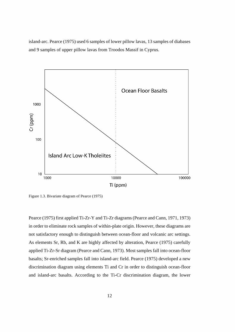
12
island-arc. Pearce (1975) used 6 samples of lower pillow lavas, 13 samples of diabases
and 9 samples of upper pillow lavas from Troodos Massif in Cyprus.
Figure 1.3. Bivariate diagram of Pearce (1975)
Pearce (1975) first applied Ti-Zr-Y and Ti-Zr diagrams (Pearce and Cann, 1971, 1973)
in order to eliminate rock samples of within-plate origin. However, these diagrams are
not satisfactory enough to distinguish between ocean-floor and volcanic arc settings.
As elements Sr, Rb, and K are highly affected by alteration, Pearce (1975) carefully
applied Ti-Zr-Sr diagram (Pearce and Cann, 1973). Most samples fall into ocean-floor
basalts; Sr-enriched samples fall into island-arc field. Pearce (1975) developed a new
discrimination diagram using elements Ti and Cr in order to distinguish ocean-floor
and island-arc basalts. According to the Ti-Cr discrimination diagram, the lower
13
pillow lavas and diabases of the Troodos Massif fall into both ocean-floor basalts and
island arc tholeiites, whereas the upper pillow lavas have low Cr concentrations
indicating an island-arc origin as previously defined by Miyashiro (1973). He used
samples from Pearce and Cann (1973) to construct a bivariate diagram of Ti-Cr in
order to discriminate ocean-floor basalts (OFB) and island arc low-K tholeiites (LKT).
The importance of Ti is its relative insensitivity to secondary processes (Cann, 1970).
Cr is also not largely affected by alteration (Bloxam and Levis, 1972) and a good
discriminator between ocean floor and island-arc basalts (Figure 1.3).
Pearce and Gale (1977) studied the tectonic environments of formation of
volcanogenic massive sulfide deposits and porphyry tin and copper deposits. They
considered stable trace element geochemistry of meta-basalts in these deposits
(especially Ti, Zr, Y, Nb, Cr and rare earth elements) and suggested a bivariate
diagram of Ti/Y versus Zr/Y (Figure 1.4) in order to discriminate two grouped tectonic
settings from each other using a dividing line; which are the combination of different
tectonic settings: plate margins including island arcs and mid-ocean ridges (ocean-
floor basalts) or within-plates including rifts and ocean island settings. This diagram
is analogous to the Ti-Zr-Y diagram of Pearce and Cann (1973).
Pearce and Norry (1979) used analysis data of HFSE (High-Field Strength Elements)
along with Ti, Zr, Y, and Nb from mafic and volcanic rocks. By the comparison of the
results of these analyses, they published a new discrimination diagram using Zr/Y
ratio and Zr (Figure 1.5). This element ratio to element diagram has a logarithmic scale
in both axes and discriminated between island-arc, MOR and within-plate settings. On
the diagram, Zr content increases from island-arc and mid-oceanic ridge towards
within-plate basalts. Island-arc basalts, though some overlap exists, have lower Zr and
Zr/Y ratio with respect to mid-ocean ridge basalts. Alkali basalts both in mid-ocean
ridges and within-plate regimes have the highest Zr/Y ratios. This element ratio-ratio
bivariate diagram is still widely applied for discrimination of these settings.
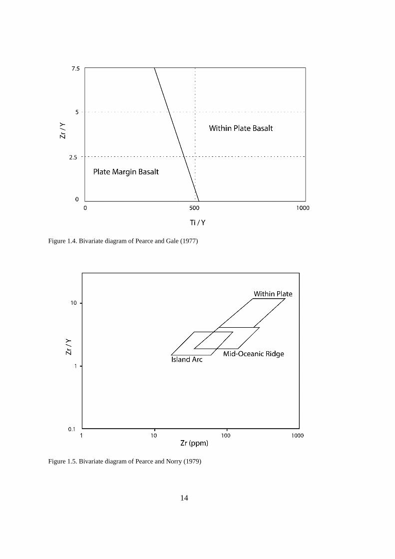
14
Figure 1.4. Bivariate diagram of Pearce and Gale (1977)
Figure 1.5. Bivariate diagram of Pearce and Norry (1979)
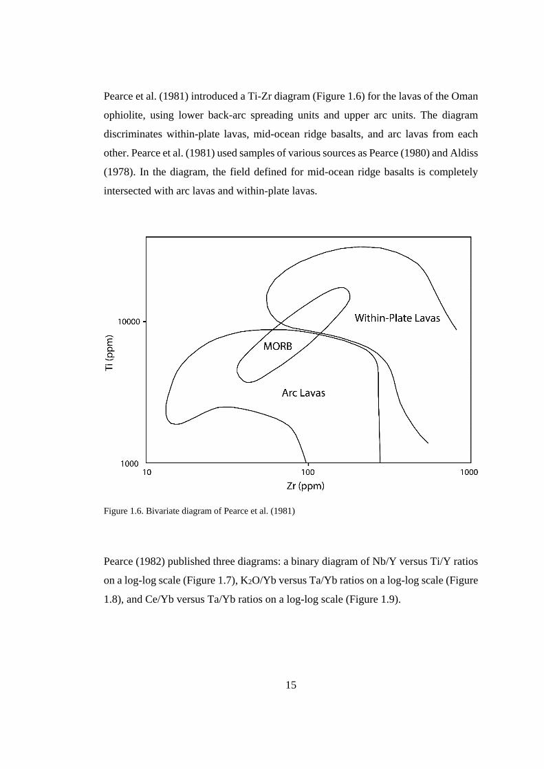
15
Pearce et al. (1981) introduced a Ti-Zr diagram (Figure 1.6) for the lavas of the Oman
ophiolite, using lower back-arc spreading units and upper arc units. The diagram
discriminates within-plate lavas, mid-ocean ridge basalts, and arc lavas from each
other. Pearce et al. (1981) used samples of various sources as Pearce (1980) and Aldiss
(1978). In the diagram, the field defined for mid-ocean ridge basalts is completely
intersected with arc lavas and within-plate lavas.
Figure 1.6. Bivariate diagram of Pearce et al. (1981)
Pearce (1982) published three diagrams: a binary diagram of Nb/Y versus Ti/Y ratios
on a log-log scale (Figure 1.7), K2O/Yb versus Ta/Yb ratios on a log-log scale (Figure
1.8), and Ce/Yb versus Ta/Yb ratios on a log-log scale (Figure 1.9).
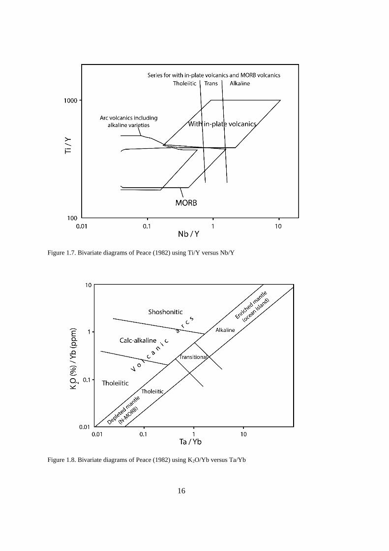
16
Figure 1.7. Bivariate diagrams of Peace (1982) using Ti/Y versus Nb/Y
Figure 1.8. Bivariate diagrams of Peace (1982) using K2O/Yb versus Ta/Yb
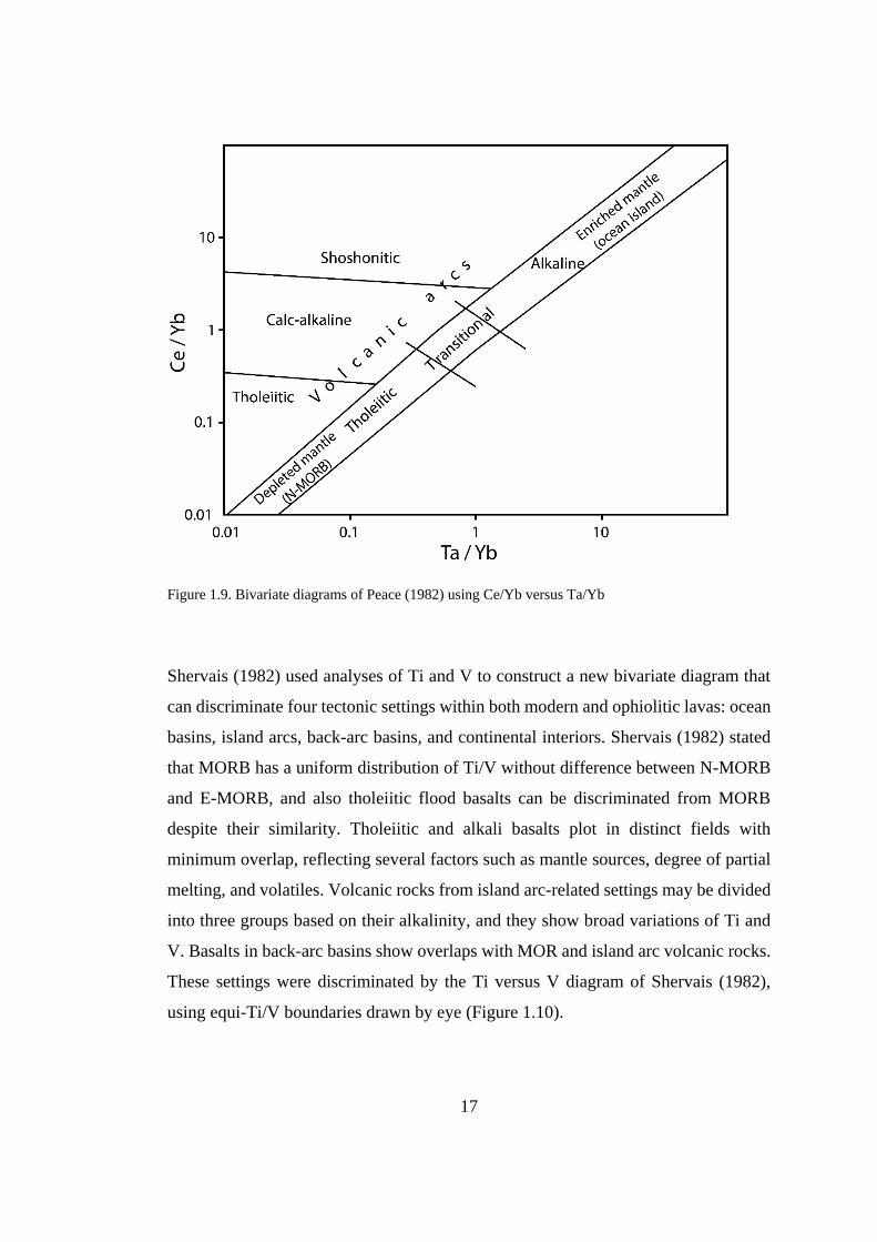
17
Figure 1.9. Bivariate diagrams of Peace (1982) using Ce/Yb versus Ta/Yb
Shervais (1982) used analyses of Ti and V to construct a new bivariate diagram that
can discriminate four tectonic settings within both modern and ophiolitic lavas: ocean
basins, island arcs, back-arc basins, and continental interiors. Shervais (1982) stated
that MORB has a uniform distribution of Ti/V without difference between N-MORB
and E-MORB, and also tholeiitic flood basalts can be discriminated from MORB
despite their similarity. Tholeiitic and alkali basalts plot in distinct fields with
minimum overlap, reflecting several factors such as mantle sources, degree of partial
melting, and volatiles. Volcanic rocks from island arc-related settings may be divided
into three groups based on their alkalinity, and they show broad variations of Ti and
V. Basalts in back-arc basins show overlaps with MOR and island arc volcanic rocks.
These settings were discriminated by the Ti versus V diagram of Shervais (1982),
using equi-Ti/V boundaries drawn by eye (Figure 1.10).
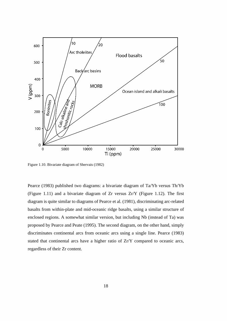
18
Figure 1.10. Bivariate diagram of Shervais (1982)
Pearce (1983) published two diagrams: a bivariate diagram of Ta/Yb versus Th/Yb
(Figure 1.11) and a bivariate diagram of Zr versus Zr/Y (Figure 1.12). The first
diagram is quite similar to diagrams of Pearce et al. (1981), discriminating arc-related
basalts from within-plate and mid-oceanic ridge basalts, using a similar structure of
enclosed regions. A somewhat similar version, but including Nb (instead of Ta) was
proposed by Pearce and Peate (1995). The second diagram, on the other hand, simply
discriminates continental arcs from oceanic arcs using a single line. Pearce (1983)
stated that continental arcs have a higher ratio of Zr/Y compared to oceanic arcs,
regardless of their Zr content.
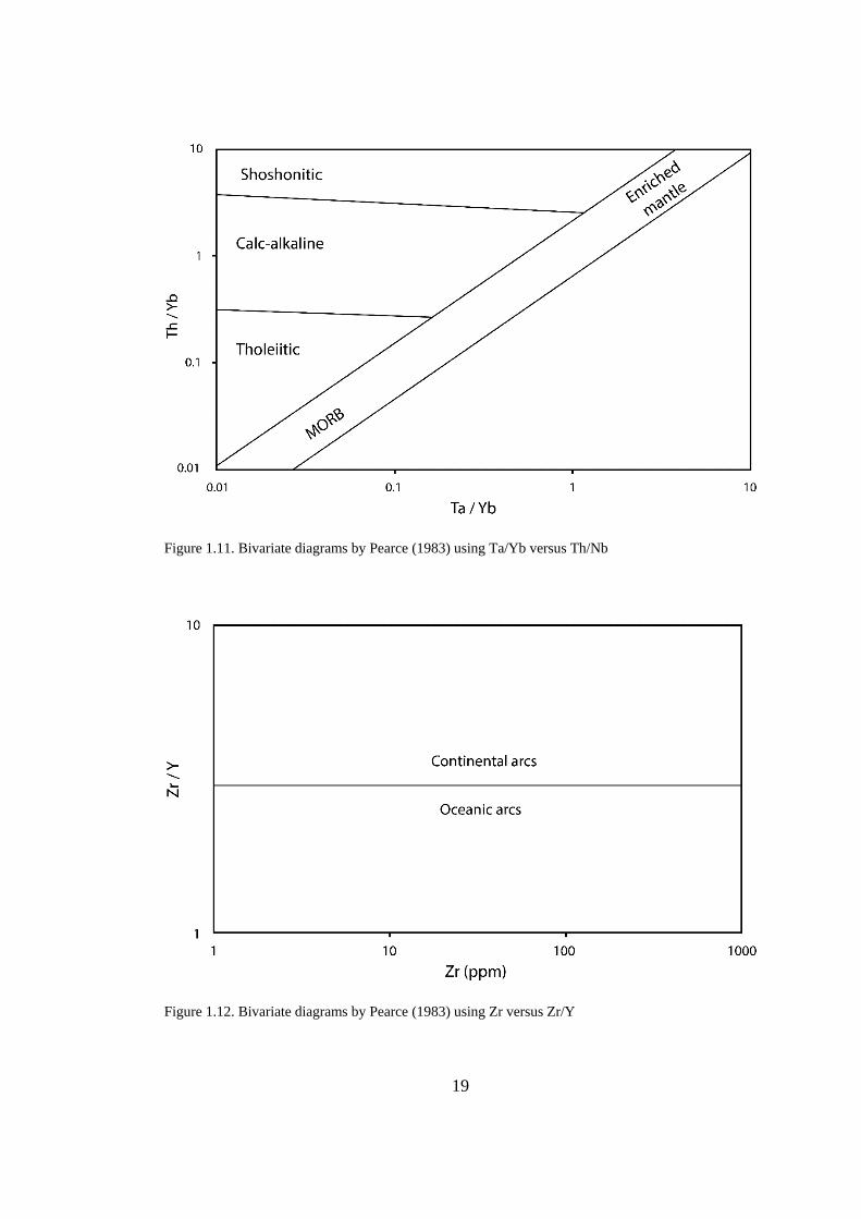
19
Figure 1.11. Bivariate diagrams by Pearce (1983) using Ta/Yb versus Th/Nb
Figure 1.12. Bivariate diagrams by Pearce (1983) using Zr versus Zr/Y
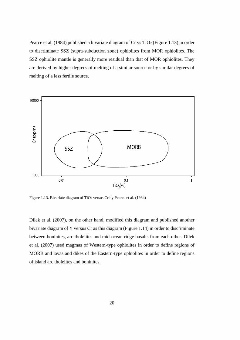
20
Pearce et al. (1984) published a bivariate diagram of Cr vs TiO2 (Figure 1.13) in order
to discriminate SSZ (supra-subduction zone) ophiolites from MOR ophiolites. The
SSZ ophiolite mantle is generally more residual than that of MOR ophiolites. They
are derived by higher degrees of melting of a similar source or by similar degrees of
melting of a less fertile source.
Figure 1.13. Bivariate diagram of TiO2 versus Cr by Pearce et al. (1984)
Dilek et al. (2007), on the other hand, modified this diagram and published another
bivariate diagram of Y versus Cr as this diagram (Figure 1.14) in order to discriminate
between boninites, arc tholeiites and mid-ocean ridge basalts from each other. Dilek
et al. (2007) used magmas of Western-type ophiolites in order to define regions of
MORB and lavas and dikes of the Eastern-type ophiolites in order to define regions
of island arc tholeiites and boninites.

21
Figure 1.14. Bivariate diagram of Y versus Cr by Dilek et al. (2007)
Hollocher et al. (2012) published two bivariate diagrams (Figure 1.15 and Figure 1.16)
in order to discriminate mid-oceanic ridge basalts, ocean islands and a variety of arc-
type basalts from each other. Hollocher et al. (2012) used the analysis results of the
samples from the Upper Allochthon metamorphosed igneous rocks of the
Scandinavian Caledonides in Norway over a large region with well-defined but
discontinuous units, for which analysis data were taken from PetDB. Data were
filtered in order to include only volcanic glass with a SiO2 range of 45-55%. Element
conversion using a conversion factor was applied in order to increase the number of
samples plotted in diagrams. The filtered dataset included 1.586 mid-oceanic ridge
basalts, 518 oceanic-arc and 1.793 continental arc, 1.021 alkaline arc, 958 back-arc
basin, and 2.438 ocean island samples. Discriminant lines were drawn by eye with
wide overlapping fields.
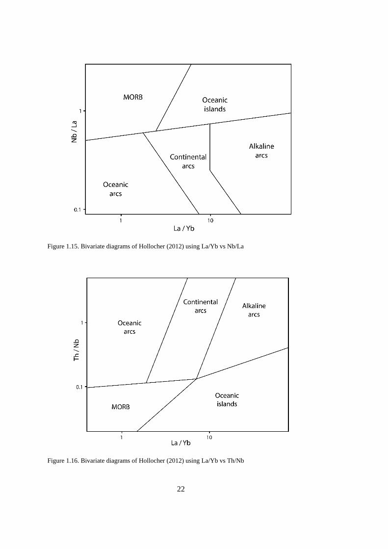
22
Figure 1.15. Bivariate diagrams of Hollocher (2012) using La/Yb vs Nb/La
Figure 1.16. Bivariate diagrams of Hollocher (2012) using La/Yb vs Th/Nb

23
Saccani (2015) published a new bivariate tectonomagmatic discrimination diagram
using N-MORB-normalized values of Th and Nb for the tectonomagmatic
discrimination of different ophiolitic basalts (Figure 1.17). More than 2000 ophiolitic
basalts from ten different basalt localities were used in order to obtain this diagram.
The diagram is used for discrimination of convergent and divergent plate settings from
each other and also discrimination of back-arcs, subduction unrelated settings and
rifted margins, fore-arcs, intra-arcs, island arcs and volcanic arcs.
Figure 1.17. Bivariate diagrams of Saccani (2015) using normalized values of Th versus Nb
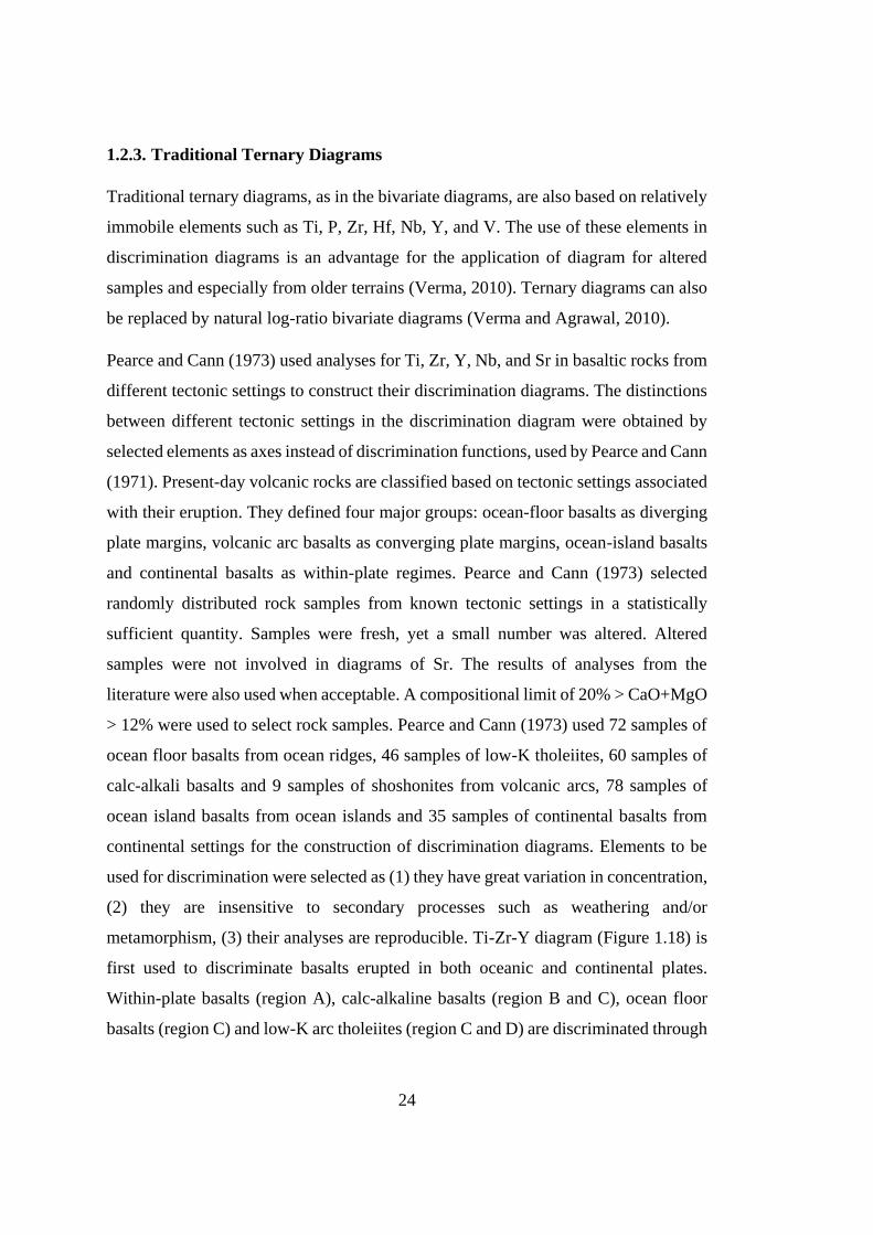
24
1.2.3. Traditional Ternary Diagrams
Traditional ternary diagrams, as in the bivariate diagrams, are also based on relatively
immobile elements such as Ti, P, Zr, Hf, Nb, Y, and V. The use of these elements in
discrimination diagrams is an advantage for the application of diagram for altered
samples and especially from older terrains (Verma, 2010). Ternary diagrams can also
be replaced by natural log-ratio bivariate diagrams (Verma and Agrawal, 2010).
Pearce and Cann (1973) used analyses for Ti, Zr, Y, Nb, and Sr in basaltic rocks from
different tectonic settings to construct their discrimination diagrams. The distinctions
between different tectonic settings in the discrimination diagram were obtained by
selected elements as axes instead of discrimination functions, used by Pearce and Cann
(1971). Present-day volcanic rocks are classified based on tectonic settings associated
with their eruption. They defined four major groups: ocean-floor basalts as diverging
plate margins, volcanic arc basalts as converging plate margins, ocean-island basalts
and continental basalts as within-plate regimes. Pearce and Cann (1973) selected
randomly distributed rock samples from known tectonic settings in a statistically
sufficient quantity. Samples were fresh, yet a small number was altered. Altered
samples were not involved in diagrams of Sr. The results of analyses from the
literature were also used when acceptable. A compositional limit of 20% > CaO+MgO
> 12% were used to select rock samples. Pearce and Cann (1973) used 72 samples of
ocean floor basalts from ocean ridges, 46 samples of low-K tholeiites, 60 samples of
calc-alkali basalts and 9 samples of shoshonites from volcanic arcs, 78 samples of
ocean island basalts from ocean islands and 35 samples of continental basalts from
continental settings for the construction of discrimination diagrams. Elements to be
used for discrimination were selected as (1) they have great variation in concentration,
(2) they are insensitive to secondary processes such as weathering and/or
metamorphism, (3) their analyses are reproducible. Ti-Zr-Y diagram (Figure 1.18) is
first used to discriminate basalts erupted in both oceanic and continental plates.
Within-plate basalts (region A), calc-alkaline basalts (region B and C), ocean floor
basalts (region C) and low-K arc tholeiites (region C and D) are discriminated through

25
this diagram. For the rock samples not classified as “within-plate basalt” by
discrimination by the Ti-Zr-Y diagram, Pearce and Cann (1973) established another
ternary diagram using Ti-Zr-Sr (Figure 1.19). Tectonic discrimination diagrams are
much more efficient when constructed based on stable elements as they are not easily
affected by secondary processes such as weathering and metamorphism (Pearce,
1975). The discrimination diagrams of Pearce and Cann (1971, 1973) are highly
efficient for distinguishing magma types as they use stable elements Ti, Zr, Y, and
Nb. Cr is another fairly stable element which is resistant to alteration (Bloxam and
Levis, 1972).
Figure 1.18. Discrimination diagrams of Pearce and Cann (1973) using Ti/100-Zr-Y*3
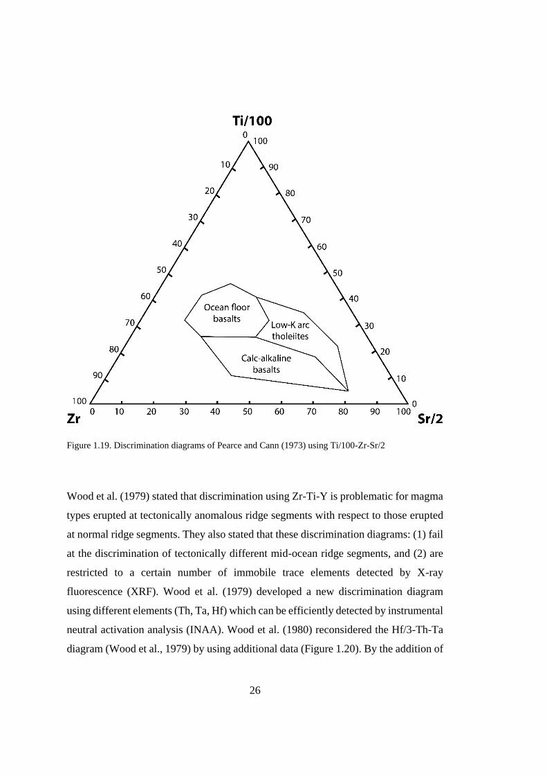
26
Figure 1.19. Discrimination diagrams of Pearce and Cann (1973) using Ti/100-Zr-Sr/2
Wood et al. (1979) stated that discrimination using Zr-Ti-Y is problematic for magma
types erupted at tectonically anomalous ridge segments with respect to those erupted
at normal ridge segments. They also stated that these discrimination diagrams: (1) fail
at the discrimination of tectonically different mid-ocean ridge segments, and (2) are
restricted to a certain number of immobile trace elements detected by X-ray
fluorescence (XRF). Wood et al. (1979) developed a new discrimination diagram
using different elements (Th, Ta, Hf) which can be efficiently detected by instrumental
neutral activation analysis (INAA). Wood et al. (1980) reconsidered the Hf/3-Th-Ta
diagram (Wood et al., 1979) by using additional data (Figure 1.20). By the addition of

27
new data, Wood et al. (1980) modified the previous diagram so that it is possible to
discriminate calc-alkaline lavas from island arc tholeiites. Wood et al. (1980) enlarged
some fields and modified boundaries.
Figure 1.20. Discrimination diagram of Wood (1980), modified after Wood et al. (1979) using Hf/3,
Th and Nb/16
Mullen (1983) divided the entire ternary field into six regions: ocean-island tholeiites
(region A), mid-oceanic ridge basalts (region B), island arc tholeiites (region C),
boninites (region D), calc-alkaline basalts (region E) and ocean-island alkali basalts
(region F) using basic and ultrabasic rocks from different oceanic tectonic settings
(Figure 1.21). Boninites and calc-alkaline basalt fields are not divided from each other
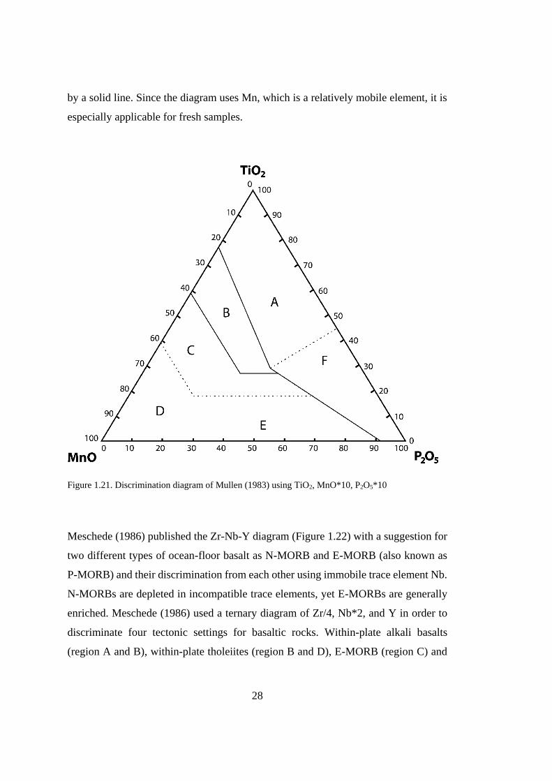
28
by a solid line. Since the diagram uses Mn, which is a relatively mobile element, it is
especially applicable for fresh samples.
Figure 1.21. Discrimination diagram of Mullen (1983) using TiO2, MnO*10, P2O5*10
Meschede (1986) published the Zr-Nb-Y diagram (Figure 1.22) with a suggestion for
two different types of ocean-floor basalt as N-MORB and E-MORB (also known as
P-MORB) and their discrimination from each other using immobile trace element Nb.
N-MORBs are depleted in incompatible trace elements, yet E-MORBs are generally
enriched. Meschede (1986) used a ternary diagram of Zr/4, Nb*2, and Y in order to
discriminate four tectonic settings for basaltic rocks. Within-plate alkali basalts
(region A and B), within-plate tholeiites (region B and D), E-MORB (region C) and
29
N-MORB (region E) are discriminated through this diagram. The fields for these
settings were defined on the basis of 1800 analyses of modern basalts with a
compositional range between 12 and 20 for CaO + MgO. The fields are within-plate
alkali basalts, within-plate tholeiites, E-MORB, N-MORB, and volcanic arc basalts.
Figure 1.22. Discrimination diagram of Meschede (1986) using 2*Nb, Zr/4 and Y
Cabanis and Lecolle (1989) used a comparatively small number of samples in order
to publish a tectonic discrimination diagram on a ternary plot of La-Y-Nb
concentrations (Figure 1.23). The diagram is used for the discrimination between
volcanic arc basalts, continental basalts, and oceanic basalts. Volcanic arc basalts are
subdivided into two groups: calc-alkali basalts and island-arc tholeiites. The settings
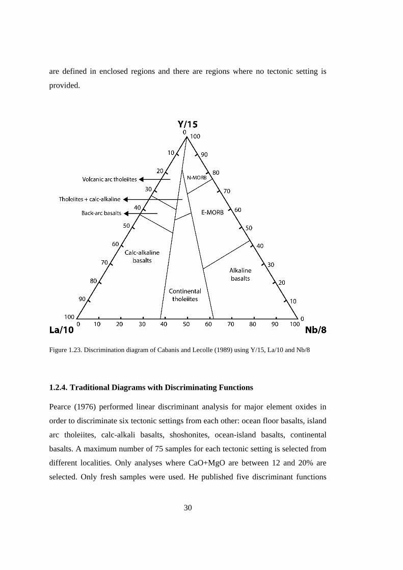
30
are defined in enclosed regions and there are regions where no tectonic setting is
provided.
Figure 1.23. Discrimination diagram of Cabanis and Lecolle (1989) using Y/15, La/10 and Nb/8
1.2.4. Traditional Diagrams with Discriminating Functions
Pearce (1976) performed linear discriminant analysis for major element oxides in
order to discriminate six tectonic settings from each other: ocean floor basalts, island
arc tholeiites, calc-alkali basalts, shoshonites, ocean-island basalts, continental
basalts. A maximum number of 75 samples for each tectonic setting is selected from
different localities. Only analyses where CaO+MgO are between 12 and 20% are
selected. Only fresh samples were used. He published five discriminant functions

31
(Table 1.1). based on major element oxides (DF1, DF2, DF3, DF4, and DF5) and
presented two discrimination diagrams based on DF1-DF2 DF3 (Figure 1.24) and
DF1-DF3 (Figure 1.25).
Table 1.1. Discrimination functions used in diagrams of Pearce (1976)
Discrimination Functions
DF1 +0.0088SiO2-0.0774TiO2+0.0102Al2O3+0.0066FeO-0.0017MgO-0.0143CaO-
0.0155Na2O-0.0007K2O
DF2 -0.0130SiO2-0.0185TiO2-0.0129Al2O3-0.0134FeO-0.0300MgO-0.0204CaO-
0.0481Na2O+0.0715K2O
DF3 -0.221SiO2-0.0532TiO2-0.0361Al2O3-0.0016FeO-0.0310MgO-0.0237CaO-
0.0614Na2O-0.0289K2O
Figure 1.24. Discrimination diagrams of Pearce (1976) using DF1 and DF2

32
Figure 1.25. Discrimination diagrams of Pearce (1976) using DF2 and DF3
Butler and Woronow (1986) proposed an alternative approach to the tectonic
discrimination of igneous rocks by using principal component analysis. They created
a bivariate graph which uses two principal components (Table 1.2) in the form of
functions of Ti, Zr, Y, and Sr (Figure 1.26). The settings discriminated in this graph
are similar to Pearce and Cann (1973), yet this graph is accepted to be more
mathematical with respect to the original Ti-Zr-Y diagram.
Table 1.2. Discrimination functions used in diagrams of Butler and Woronow (1986)
Discrimination Functions
Score 1 0.3707Ti-0.0668Zr-0.398Y+0.8362Sr
Score 2 -0.3376Ti-0.5602Zr+0.7397Y +0.1582Sr

33
Figure 1.26. Discrimination diagrams of Pearce (1976) using DF1 and DF2
Velikonslavinsky and Kykrylov (2014) published new tectono-magmatic
discrimination diagrams (Figure 1.27) for basalts from tectonic settings of island-arcs,
within-plates, mid-ocean ridges, and post-collisional settings using discrimination
functions (Table 1.3). They used a database from global geochemical datasets such as
GEOROC, PetDB, IGBA, RidgeDB. They used a two-stage discrimination. At first
stage, they discriminate WPB, IAB and MOR creating discriminating functions with
combinations of elements including major oxides (SiO2, TiO2, Al2O3, FeO* (total iron
in form of FeO), MgO, CaO, Na2O, K2O, P2O5, Rb, Sr, Y, Zr, Nb, La, Ce, Nd, Sm,
Eu, and Yb). At the second stage, PCB (basalts of post-collisional setting) is separated
with discriminating functions by a combination of major oxides and minor elements
(Rb, Sr, Y, Zr, and Nb).
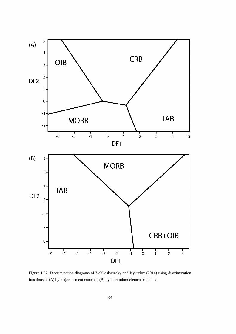
34
Figure 1.27. Discrimination diagrams of Velikoslavinsky and Kykrylov (2014) using discrimination
functions of (A) by major element contents, (B) by inert minor element contents
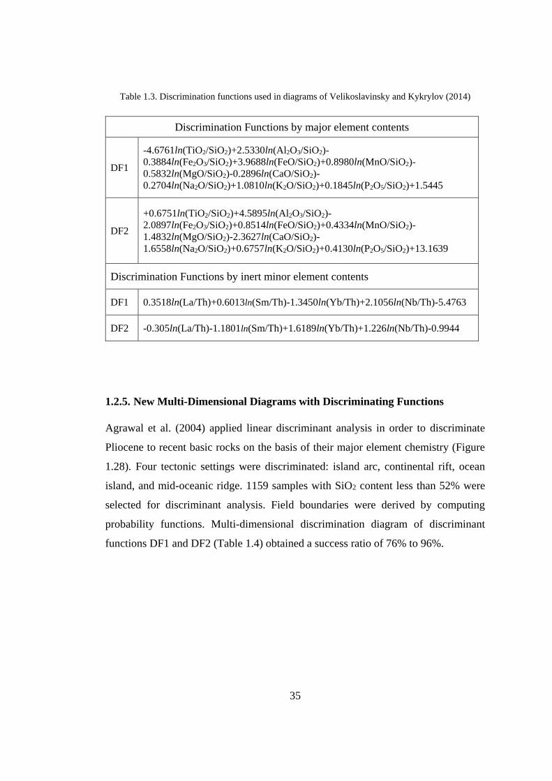
35
Table 1.3. Discrimination functions used in diagrams of Velikoslavinsky and Kykrylov (2014)
Discrimination Functions by major element contents
DF1
-4.6761ln(TiO2/SiO2)+2.5330ln(Al2O3/SiO2)-
0.3884ln(Fe2O3/SiO2)+3.9688ln(FeO/SiO2)+0.8980ln(MnO/SiO2)-
0.5832ln(MgO/SiO2)-0.2896ln(CaO/SiO2)-
0.2704ln(Na2O/SiO2)+1.0810ln(K2O/SiO2)+0.1845ln(P2O5/SiO2)+1.5445
DF2
+0.6751ln(TiO2/SiO2)+4.5895ln(Al2O3/SiO2)-
2.0897ln(Fe2O3/SiO2)+0.8514ln(FeO/SiO2)+0.4334ln(MnO/SiO2)-
1.4832ln(MgO/SiO2)-2.3627ln(CaO/SiO2)-
1.6558ln(Na2O/SiO2)+0.6757ln(K2O/SiO2)+0.4130ln(P2O5/SiO2)+13.1639
Discrimination Functions by inert minor element contents
DF1 0.3518ln(La/Th)+0.6013ln(Sm/Th)-1.3450ln(Yb/Th)+2.1056ln(Nb/Th)-5.4763
DF2 -0.305ln(La/Th)-1.1801ln(Sm/Th)+1.6189ln(Yb/Th)+1.226ln(Nb/Th)-0.9944
1.2.5. New Multi-Dimensional Diagrams with Discriminating Functions
Agrawal et al. (2004) applied linear discriminant analysis in order to discriminate
Pliocene to recent basic rocks on the basis of their major element chemistry (Figure
1.28). Four tectonic settings were discriminated: island arc, continental rift, ocean
island, and mid-oceanic ridge. 1159 samples with SiO2 content less than 52% were
selected for discriminant analysis. Field boundaries were derived by computing
probability functions. Multi-dimensional discrimination diagram of discriminant
functions DF1 and DF2 (Table 1.4) obtained a success ratio of 76% to 96%.
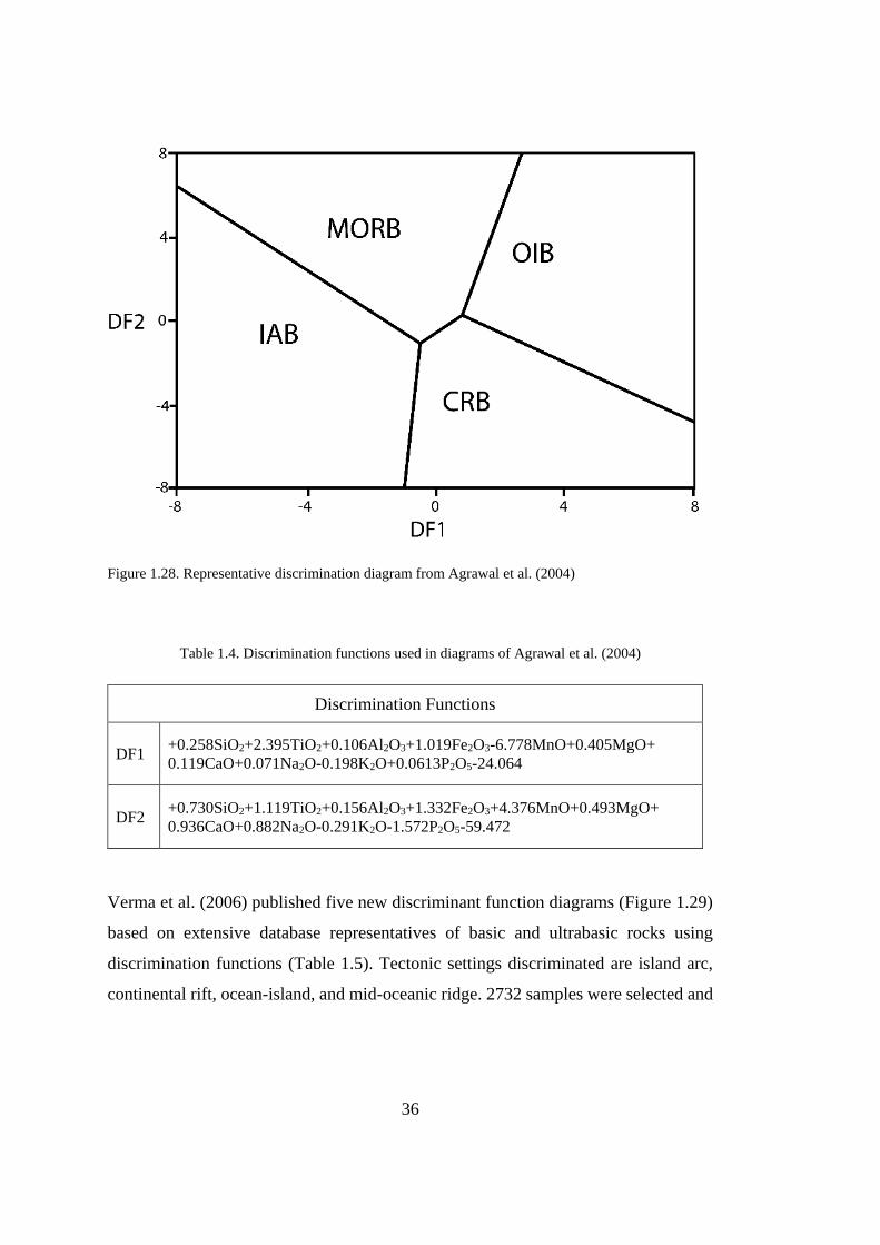
36
Figure 1.28. Representative discrimination diagram from Agrawal et al. (2004)
Table 1.4. Discrimination functions used in diagrams of Agrawal et al. (2004)
Discrimination Functions
DF1 +0.258SiO2+2.395TiO2+0.106Al2O3+1.019Fe2O3-6.778MnO+0.405MgO+
0.119CaO+0.071Na2O-0.198K2O+0.0613P2O5-24.064
DF2 +0.730SiO2+1.119TiO2+0.156Al2O3+1.332Fe2O3+4.376MnO+0.493MgO+
0.936CaO+0.882Na2O-0.291K2O-1.572P2O5-59.472
Verma et al. (2006) published five new discriminant function diagrams (Figure 1.29)
based on extensive database representatives of basic and ultrabasic rocks using
discrimination functions (Table 1.5). Tectonic settings discriminated are island arc,
continental rift, ocean-island, and mid-oceanic ridge. 2732 samples were selected and
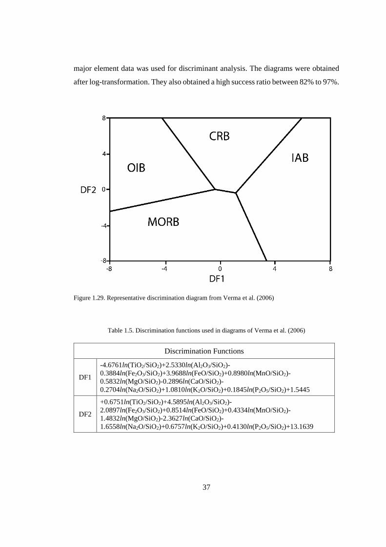
37
major element data was used for discriminant analysis. The diagrams were obtained
after log-transformation. They also obtained a high success ratio between 82% to 97%.
Figure 1.29. Representative discrimination diagram from Verma et al. (2006)
Table 1.5. Discrimination functions used in diagrams of Verma et al. (2006)
Discrimination Functions
DF1
-4.6761ln(TiO2/SiO2)+2.5330ln(Al2O3/SiO2)-
0.3884ln(Fe2O3/SiO2)+3.9688ln(FeO/SiO2)+0.8980ln(MnO/SiO2)-
0.5832ln(MgO/SiO2)-0.2896ln(CaO/SiO2)-
0.2704ln(Na2O/SiO2)+1.0810ln(K2O/SiO2)+0.1845ln(P2O5/SiO2)+1.5445
DF2
+0.6751ln(TiO2/SiO2)+4.5895ln(Al2O3/SiO2)-
2.0897ln(Fe2O3/SiO2)+0.8514ln(FeO/SiO2)+0.4334ln(MnO/SiO2)-
1.4832ln(MgO/SiO2)-2.3627ln(CaO/SiO2)-
1.6558ln(Na2O/SiO2)+0.6757ln(K2O/SiO2)+0.4130ln(P2O5/SiO2)+13.1639
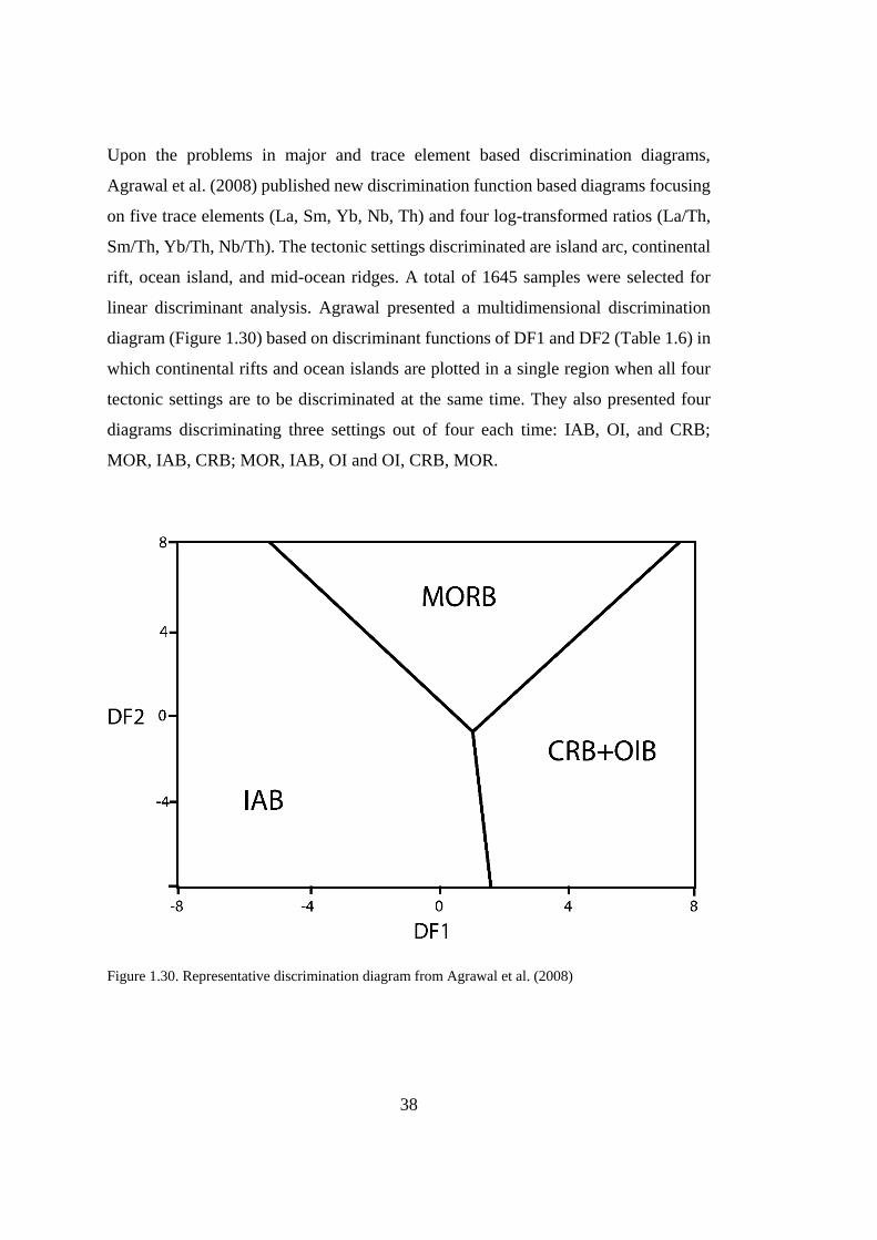
38
Upon the problems in major and trace element based discrimination diagrams,
Agrawal et al. (2008) published new discrimination function based diagrams focusing
on five trace elements (La, Sm, Yb, Nb, Th) and four log-transformed ratios (La/Th,
Sm/Th, Yb/Th, Nb/Th). The tectonic settings discriminated are island arc, continental
rift, ocean island, and mid-ocean ridges. A total of 1645 samples were selected for
linear discriminant analysis. Agrawal presented a multidimensional discrimination
diagram (Figure 1.30) based on discriminant functions of DF1 and DF2 (Table 1.6) in
which continental rifts and ocean islands are plotted in a single region when all four
tectonic settings are to be discriminated at the same time. They also presented four
diagrams discriminating three settings out of four each time: IAB, OI, and CRB;
MOR, IAB, CRB; MOR, IAB, OI and OI, CRB, MOR.
Figure 1.30. Representative discrimination diagram from Agrawal et al. (2008)

39
Table 1.6. Discrimination functions used in diagrams of Verma et al. (2006)
Discrimination Functions
DF1 0.3518ln(La/Th)+0.6013ln(Sm/Th)-1.3450ln(Yb/Th)+2.1056ln(Nb/Th)-5.4763
DF2 -0.305ln(La/Th)-1.1801ln(Sm/Th)+1.6189ln(Yb/Th)+1.226ln(Nb/Th)-0.9944
Verma and Agrawal (2011) published new tectonic discrimination diagrams for basic
and ultrabasic volcanic rocks (Figure 1.31). They applied log-transformation to five
HFSE: TiO2, Nb, V, Y, and Zr. The database was compiled from previous studies of
Verma et al. (2006), Agrawal et al. (2004, 2008), and Verma (2010). 1877 analyses
were used for discriminant analysis. The tectonic settings discriminated are island
arcs, continental rifts, ocean-islands, and mid-ocean ridges. Five HFSE elements and
their log-transformed ratios (Nb/TiO2, V/TiO2, Y/TiO2, and Zr/TiO2) were used in
discriminant functions obtaining success ratios between 80% and 94%. Verma and
Agrawal (2011) also published one diagram in which continental rifts and ocean
islands are plotted on the same region and four diagrams their triple combinations of
four tectonic settings were discriminated separately.
1.2.6. Discrimination using Machine Learning Methods
Vermeesch (2006a) used the decision tree learning method of machine learning and
built two decision trees in order to discriminate between three different tectonic
settings for basaltic rocks; mid-ocean ridges, ocean islands, and island arcs. He used
756 samples from global geochemical datasets of PetDB and GEOROC with their
major and trace element and isotope ratio measurements in order to build decision
trees. The first tree uses all samples with all elements and isotope ratios (Figure 1.32).
The second one only uses altered samples and immobile elements, thus expected to be
resistant against weathering and/or metamorphism (Figure 1.33). He stated that the
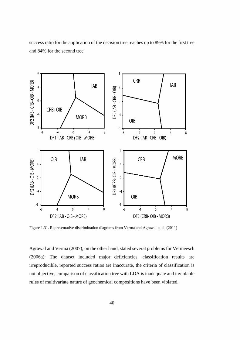
40
success ratio for the application of the decision tree reaches up to 89% for the first tree
and 84% for the second tree.
Figure 1.31. Representative discrimination diagrams from Verma and Agrawal et al. (2011)
Agrawal and Verma (2007), on the other hand, stated several problems for Vermeesch
(2006a): The dataset included major deficiencies, classification results are
irreproducible, reported success ratios are inaccurate, the criteria of classification is
not objective, comparison of classification tree with LDA is inadequate and inviolable
rules of multivariate nature of geochemical compositions have been violated.
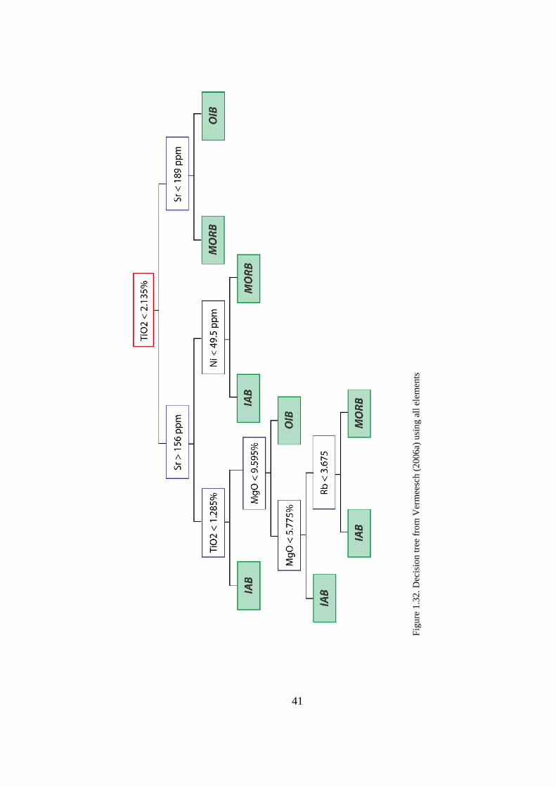
41
Figure 1.32. Decision tree from Vermeesch (2006a) using all elements
Fig
ure
1.3
2. D
ecis
ion
tre
e fr
om
Ver
mee
sch
(2
006
a) u
sin
g a
ll e
lem
ents
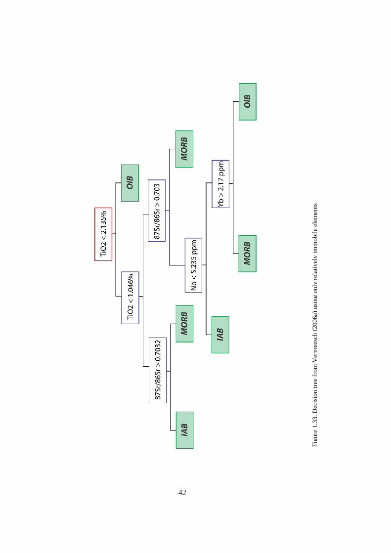
42
Figure 1.33. Decision tree from Vermeesch (2006a) using only relatively immobile elements
Fig
ure
1.3
3. D
ecis
ion
tre
e fr
om
Ver
mee
sch
(2
006
a) u
sin
g o
nly
rel
ativ
ely i
mm
ob
ile
elem
ents

43
Ueki (2017) applied three different machine learning techniques (support vector
machine, sparse multinomial regression, and random forest) in order to discriminate
magmas from eight different tectonic settings using representative basalt compositions
from global geochemical datasets (PetDB and GEOROC). Data published before 1990
were eliminated in order to prevent analytical uncertainties, and outliers were
excluded. The samples from problematic localities such as Azores, the Galapagos,
Iceland, and Chile, etc) were eliminated. A total of 2074 samples were used for
discrimination. The tectonic settings to be discriminated are back-arc basins,
continental arcs, continental floods, island arcs, intra-oceanic arcs, mid-oceanic
ridges, oceanic islands, and oceanic plateaus. For discrimination, 20 elements
including major elements (SiO2, TiO2, Al2O3, Fe2O3, CaO, MgO, Na2O, K2O), along
with selected trace element (Sr, Ba, Rb, Zr, Nb, La, Ce, Nd, Hf, Sm, Gd, Y, Yb, Lu,
Ta, Th) and 5 isotopic ratios (206Pb/204Pb, 207Pb/204Pb, 208Pb/204Pb, 87Sr/86Sr and
143Nd/144Nd) were used. Ueki used geochemical compositional data normalized using
a one-parameter Box-Cox transform before the application of machine learning
algorithms. The performance of discriminations obtained by machine learning
techniques was evaluated by 10-fold cross-validation. Ueki showed that modern
techniques of machine learning can be a better option for tectono-magmatic
discrimination of igneous rocks having high success ratios for support vector machine,
sparse multinomial regression, and random forest.
These modern techniques of machine learning along with the traditional methods are
still being tested by other researchers (Verma, 2017; Gomez and Verma, 2016; Verma
and Oliveira, 2015; Verma et al., 2015; Li, 2015, Pandarinath, 2014; Pandarinath and
Verma, 2013, Verma et al., 2012; Verma, 2010; Sheth, 2008) and compared with
traditional discrimination methods (bivariate and ternary diagrams)..

45
CHAPTER 2
2. DATABASE AND METHODOLOGY
2.1. Data Gathering and Import
The complete database is compiled for 5,114 samples of mainly basic and to a lesser
extent ultrabasic igneous rocks from known locations of uncontroversial tectonic
settings from all over the world directly from published literature. The database
includes the articles generally published after 1995 (with some exceptions). The aim
is to include the chemical analyses with high precision and accuracy so that the ratios
would reflect the true fractionation between the elements. This is actually very critical,
since any false fractionation effect, which may have raised from analytical errors, have
the potential of misclassification of the data. Therefore, the database is constructed on
high-quality data that best reflects the true geochemical nature of the investigated
basic lithology.
The geology, lithology, mineralogy, and geochemistry of samples along with source
rock characteristics of each location are referred from the original articles. Global
geochemical databases such as GEOROC-Mainz or PetDB are avoided in the
construction of the database as they have significant errors that may result in false
interpretations (Gomez and Verma, 2016).
2.2. Data Cleaning
The database initially included all available samples from related articles. However, a
variety of samples are eliminated in three-stages based on certain criteria.
46
Initially, the problematic samples are eliminated from the database. Some of the
problematic samples include non-igneous lithologies. These are characterized by
sedimentary or metamorphic samples, which are analyzed to get petrogenetic
inferences, such as slab-derived contributions, nature of the source, crustal
contamination. Some other problematic samples, however, are characterized by
apparent numerical inconsistencies with the rest of the samples in the dataset, which
result in unrealistic element ratios. This problem can be related to analytical errors or
can be simply attributed to typos made during the preparation of the manuscript. If all
samples from a certain data source are problematic, then the data source is completely
removed from the database or transferred to another database.
On the second stage, the data cleaning is solely based on the rock type of samples. The
rock type is evaluated by chemical classification using the plot of LeMaitre (1987).
Since this study intends to discriminate the basic rocks, the igneous varieties included
in the database are basalts, trachybasalts, picrobasalts, foidites, tephrites/basanites.
Apart from continental arcs, there is a vast number of basaltic rocks sampled from the
other tectonic settings. Continental arcs, however, include a somewhat limited amount
of mafic compositions. The reason is mainly that continental arcs have a thick
continental lithospheric cap, which increases the change of mafic magmas to interact
with the continental crust whose composition significantly differs from that of oceanic
crust (e.g. Davidson et al.,1989; Bryant et al.,2006; Stern 2010). Thus, the increasing
interaction between continental crust and greater residence times of the magmas
within the crustal magma chambers results in the extensive fractionation of mafic
magmas, which in turn produces a significant amount of highly evolved varieties (i.e.
intermediate and silicic members) (e.g. Wilson 1989). Therefore, for continental arcs
only, basaltic andesites and basaltic trachyandesites are also included in the database
in order to increase the number of samples for this tectonic setting, which allowed to
make a better comparison by homogenizing the sample distribution. All other rock
types (i.e. intermediate and acidic varieties) are eliminated from the database at this
stage.

47
On the final stage, all samples with missing values for critical elements are eliminated
from the database. The elements, determined as “critical element” are Th, La, Nb, Y,
Yb, Zr, Hf, Sm, Nd, and TiO2, which are selected due to their petrogenetic significance
in different tectonic settings (which will be explained in the following paragraphs).
2.3. Classes (Tectonic Settings)
Classes (target features) in the database are characterized by seven tectonic settings,
namely continental arc, continental within-plate (including continental rifts and
continental flood basalts), mid-ocean ridge, oceanic arc, oceanic back-arc basin,
oceanic island, and oceanic plateau. The classification is intended to include nearly all
the tectonic settings. The continental back-arcs, however, is excluded due to the
limited number of samples available in the literature, which considerably inhibits
evaluating their petrogenetic features for discrimination. The continental back-arcs,
therefore, are ignored here for the construction of discrimination methods.
Another issue related to the classes is about oceanic back-arcs. Oceanic back-arcs
genetically stay in between the mid-ocean ridges and arcs. They begin their life by
rifting of the arcs, which can be triggered by the slab roll-back (e.g. Martinez and
Taylor, 2002; 2006). This processes result in extension and rifting of the arc, as well
as the upwelling of the asthenosphere. This stage is accompanied by diffuse
magmatism (e.g. Todd et al.,2010). The rifting and thinning of the arc crust eventually
reach a point where the oceanic crust is generated and spreading starts. Thus, the life
of an oceanic back-arc can be simply divided into two stages as rifting and spreading.
It is important to note that since the rifting back-arcs are immature (i.e not evolved to
spreading stage), they display arc-like geochemical characteristics. The spreading
back-arcs, on the other hand, are mature, and they show geochemical features between
what is called “BABB-type” and MORB-type. In this study, only spreading back-arcs
are taken into account into the evaluation, since they represent the true geochemical
nature of oceanic back-arc systems. Brief information about the tectonic settings
included in the classification is as follows:

48
- Continental arcs represent divergent plate boundaries, where the oceanic lithosphere
is subducted beneath the continental lithosphere. The generation of primary magmas
primarily occurs via flux-induced melting and may be sourced from asthenospheric
and/or continental lithospheric mantle. The presence of continental crust may add
some chemical complexities to the mantle-derived magmas en route the surface.
- Continental within-plate settings are away from the plate boundaries, and the
magmatism here does not involve any recent subduction contribution. The magmatism
can be induced by mantle plumes, which results in continental flood magmatism or
occurs via rifting (can be associated with/without plumes), resulting in continental rift
magmatism.
- Mid-oceanic ridges represent divergent plate boundaries where the two lithospheric
are moving apart from each other. A great amount of oceanic lithosphere is created at
mid-ocean ridges. The magmatism is generated by adiabatic decompression melting,
which mainly leads to large degrees of melting. While most of the magmatism occurs
at the axis, some appear to be concentrated off-axis in the form of seamounts.
- Oceanic arcs are similar to continental arcs in that they also represent the convergent
plate boundaries, and subduction is involved. However, in oceanic arcs, the
subduction occurs beneath another oceanic lithosphere, so the system is entirely
oceanic (i.e. the continental lithosphere is not involved). The melting is similarly
occurring through mainly the flux-melting. Oceanic arcs are relatively simple systems
compared to the continental arcs since they do not include continental crust in their
petrogenesis.
- Oceanic back-arcs are extensional systems created behind the arcs. They are
somewhat between mid-ocean ridges and oceanic arcs. Mature back-arcs are
characterized by spreading, creating oceanic lithosphere like mid-ocean ridges.
However, because subduction is involved, unlike mid-ocean ridges, they may have a
subduction component similar to oceanic arcs. Melting takes place via flux-induced
melting and/or decompression melting.
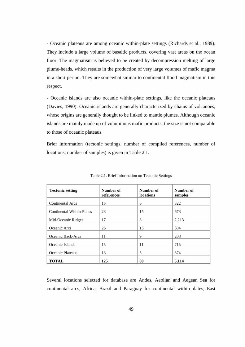
49
- Oceanic plateaus are among oceanic within-plate settings (Richards et al., 1989).
They include a large volume of basaltic products, covering vast areas on the ocean
floor. The magmatism is believed to be created by decompression melting of large
plume-heads, which results in the production of very large volumes of mafic magma
in a short period. They are somewhat similar to continental flood magmatism in this
respect.
- Oceanic islands are also oceanic within-plate settings, like the oceanic plateaus
(Davies, 1990). Oceanic islands are generally characterized by chains of volcanoes,
whose origins are generally thought to be linked to mantle plumes. Although oceanic
islands are mainly made up of voluminous mafic products, the size is not comparable
to those of oceanic plateaus.
Brief information (tectonic settings, number of compiled references, number of
locations, number of samples) is given in Table 2.1.
Table 2.1. Brief Information on Tectonic Settings
Tectonic setting Number of
references
Number of
locations
Number of
samples
Continental Arcs 15 6 322
Continental Within-Plates 28 15 678
Mid-Oceanic Ridges 17 8 2,213
Oceanic Arcs 26 15 604
Oceanic Back-Arcs 11 9 208
Oceanic Islands 15 11 715
Oceanic Plateaus 13 5 374
TOTAL 125 69 5,114
Several locations selected for database are Andes, Aeolian and Aegean Sea for
continental arcs, Africa, Brazil and Paraguay for continental within-plates, East
50
Pacific Rise, Mid-Atlantic Ridge, Indian and Atlantic Ridges for mid-oceanic ridges,
Greater and Lesser Antilles, Mariana and Vanuatu for oceanic arcs, Manus Basin, Lau
Basin and Izu Bonin for oceanic back-arcs, Hawaii, Iceland and Young Rurutu for
oceanic islands and Kerguelen, Ontong Java and Manihiki for oceanic plateaus.
2.4. Feature Selection
The database initially included all available information in related articles such as
major elements (SiO2, TiO2, Na2O, K2O, FeO / Fe2O3, MgO, MnO, CaO, Al2O3, P2O5),
minor and trace elements (Th, La, Nb, Y, Yb, Zr, Hf, Sm, Nd, Ce, Dy, Pr, Eu, Gd, Tb,
Ho, Er, Tm, Lu, Pb, Rb, Sr, Ba, Cs, Ta, U, Sc, V, Cr, Ni, Cu, Co, Sb, Zn) and isotope
ratios (87Sr/86Sr, 143Nd/144Nd, 206Pb/204Pb, 207Pb/204Pb, 208Pb/204Pb).
Although there are many elements available to consider, it is not so straightforward to
apply all of them when the effects of alteration considered. Alteration of the igneous
rock can occur during weathering or metamorphism. The igneous rocks generated at
mid-ocean ridges, for example, start experiencing hydrothermal metamorphism
immediately after their production at the ridge axis (e.g. Bach and Früh-Green, 2010).
During this process, which may involve temperatures up to ~400℃, can modify the
oceanic crustal lithologies up to amphibolite facies (e.g. Seyfried et al.,1991; Bach
and Früh-Green, 2010). With the ongoing spreading, the effect of hydrothermal
metamorphism diminishes, as the lithologies are displaced away from the ridge axis.
Following this, the alteration continues, but under very low-temperature conditions
this time (low-T alteration/weathering). The altered oceanic crust can be further
modified during subduction (e.g. Pearce and Peate, 1995; Spandler et al.,2004). The
crustal lithologies undergo dehydration with increasing temperature, and they can be
metamorphosed, for example, under blueschist to eclogite facies following a cold
subduction.
Whether it is of continental or oceanic origin, old igneous rocks are likely to be altered.
In addition, as mentioned above, some lithologies may go through multiple stages of
alteration as the fate of subducted oceanic crustal rocks. The critical thing here is that

51
the introduction of fluid phase may mobilize some elements, causing their loss or gain
in the host lithology. The mobilization is known to primarily effect the low-ionic
potential elements, such as Rb, Ba, K, Si etc. In contrast, the elements with
intermediate ionic potential, like HFSE and REE (Rare Earth Element) are mainly
known to be fluid-immobile (e.g. Pearce 1975; Staudigel et al.,1996; Bach and Früh-
Green, 2010). Although the stability of the latter group of elements (HFSE and REE)
are mostly valid under weathering and low-grade metamorphic conditions
(greenschist facies), their relative immobility have also been reported for higher-grade
metamorphic conditions (i.e. amphibolite, blueschist, and eclogite facies; Spandler et
al.,2004; John et al.,2010; Sayit et al.,2016). Mobilization may cause significant
fractionation of the mobile elements (among themselves and/or relative to immobile
ones). Their use (either as absolute abundances or ratios) should be carefully handled
or avoided when making petrogenetic inferences. Therefore, for altered rocks, the use
of fluid-immobile elements would be a better choice to infer pristine geochemical
features inherited from the protolith/original rock.
Considering the potential effects of mobilization on the altered rocks as explained
above, only the fluid-immobile elements are considered in this study. It must be noted
that most major and minor elements are known to be mobile in fluids. The most
resistant ones appear to be Ti, Al, P, and Cr. However, apart from Ti, the others can
also be mobilized to some extent under hydrothermal metamorphism (Pearce 1975).
Thus, of these, only Ti is included in this study as an element that can reflect the
pristine geochemical features under a broad spectrum of alteration conditions.
Isotope ratios are among the least used discriminators when taking into account the
tectonomagmatic discrimination methods published thus far. The only study in this
regard is that of Vermeesh (2006A), who involved 87Sr/86Sr for the decision-tree-based
tectonomagmatic discrimination. Sr isotopic ratio, however, can be strongly affected
through interaction with seawater (e.g. Bach et al.,2003), which makes it a highly
unreliable discriminator. On the other hand, Nd and Pb isotopic ratios remain
unaffected upon interaction with seawater, thus they can act as better proxies for the
52
tectonomagmatic discrimination. However, in spite of this petrogenetic superiority,
the higher analytical costs of isotopic systems make them less available for most
datasets. Also, age-correction poses another problem. Since isotopic ratios can
significantly differ from the measured ones, this issue requires the precise age for
every sample included for the petrogenetic considerations. However, providing age
data for every sample on the ancient rocks is a highly difficult job, especially regarding
the ones from the mélanges. Thus, although the isotopic ratios may serve some
invaluable information, their low applicability makes them less deserved features for
fingerprinting of the igneous rocks.
Another issue to be noted that absolute values of relatively immobile elements are
only used for calculation of ratios but not used in the construction of discrimination
methods. This is one of the critical points in this study since the Orange software is
not able to calculate the elemental ratios from the absolute abundances, which might
be suitable for the construction of decision trees. Thus, the consideration of elemental
ratios, which is believed to be of a petrogenetic significance, is devised and introduced
manually, not by the software. One of the advantages of using ratios over absolute
abundances is to minimize the effect of fractional crystallization (FC). Another strong
constraint comes from the fact that since the partitioning of fluid-immobile trace
elements is highly dependent on the residual mineralogy, they are powerful features
in reflecting petrogenetic characteristics, including the nature of mantle source region,
degree of partial melting, and contribution of subduction components (e.g. Pearce
1983; McKenzie and O’Nions 1991; Weaver 1991; Shaw 2006).
Using element ratios instead of absolute abundances also increases the discrimination
ability of constructed decision trees as an element ratio would be much more
discriminating feature when compared to absolute abundance of each element used in
calculation of ratio (e.g. Th/Nb compared to Th and Nb) (Figure 2.1).
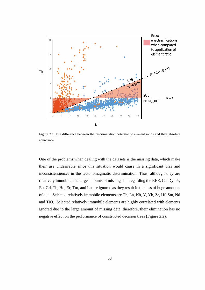
53
Figure 2.1. The difference between the discrimination potential of element ratios and their absolute
abundance
One of the problems when dealing with the datasets is the missing data, which make
their use undesirable since this situation would cause in a significant bias and
inconsistentiences in the tectonomagmatic discrimination. Thus, although they are
relatively immobile, the large amounts of missing data regarding the REE, Ce, Dy, Pr,
Eu, Gd, Tb, Ho, Er, Tm, and Lu are ignored as they result in the loss of huge amounts
of data. Selected relatively immobile elements are Th, La, Nb, Y, Yb, Zr, Hf, Sm, Nd
and TiO2. Selected relatively immobile elements are highly correlated with elements
ignored due to the large amount of missing data, therefore, their elimination has no
negative effect on the performance of constructed decision trees (Figure 2.2).
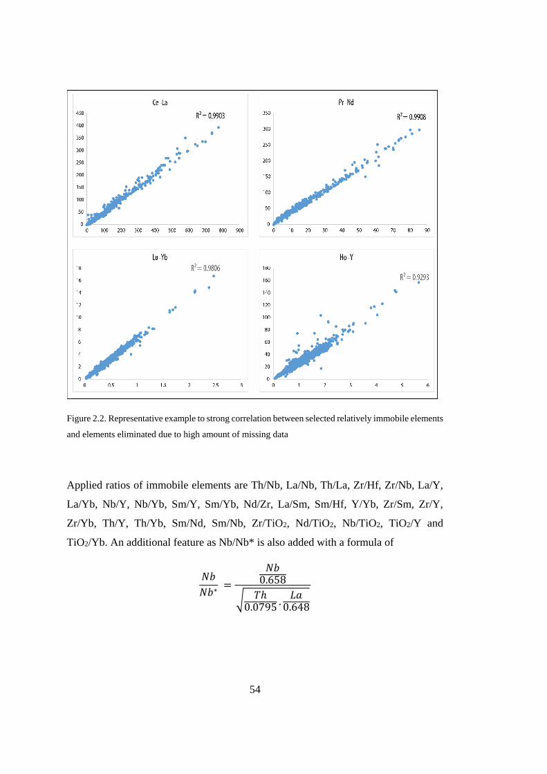
54
Figure 2.2. Representative example to strong correlation between selected relatively immobile elements
and elements eliminated due to high amount of missing data
Applied ratios of immobile elements are Th/Nb, La/Nb, Th/La, Zr/Hf, Zr/Nb, La/Y,
La/Yb, Nb/Y, Nb/Yb, Sm/Y, Sm/Yb, Nd/Zr, La/Sm, Sm/Hf, Y/Yb, Zr/Sm, Zr/Y,
Zr/Yb, Th/Y, Th/Yb, Sm/Nd, Sm/Nb, Zr/TiO2, Nd/TiO2, Nb/TiO2, TiO2/Y and
TiO2/Yb. An additional feature as Nb/Nb* is also added with a formula of
𝑁𝑏
𝑁𝑏∗ =
𝑁𝑏0.658
√ 𝑇ℎ0.0795
.𝐿𝑎
0.648

55
2.5. Splitting Database
The database is first divided into two datasets: Training-test dataset and external
dataset. Then, training-test dataset is randomly divided by Orange software as training
dataset and test dataset in proportions of 80% and 20%, with respectively. Training
dataset is the dataset used in the construction of discrimination methods. The test
dataset is the dataset similar to training dataset and used for the initial test for the
performance of discrimination methods. The external dataset is the dataset different
than the training and test datasets and used for the test for external applicability of
discrimination methods to different tectonic settings and locations all over the world.
2.6. Methodology (Decision Tree Learning)
2.6.1. Non-Mathematical Explanation of Decision Tree Learning
Data science is the discipline of processing and analyzing data for the purpose of
extracting valuable knowledge. The term “data science” was first used in the 1960s
but became popular recently with developments in technology. Various domains such
as commerce, medicine, and research are applying data-driven discovery and
prediction in order to gain some new insights, such as Google, which tracks user clicks
in order to improve its search engine results and ads.
Data science is the science of exploring data in order to discover useful patterns and
obtain valuable insights. The use of decision trees is one of the promising and popular
approaches of data science. Decision trees are simple but also successful techniques
for predicting and explaining the relationship between various features (such as
element concentration or ratio of element concentration) of an item (such as a rock)
and its target value (such as its tectonic setting).
Decision trees are multi-purpose applications especially for classification problems as
they are self-explanatory and easy to follow, flexible in handling a variety of input
data, adaptable in processing datasets with errors and missing data, and useful for large
datasets. They are successful predictors for a relatively small computational effort.

56
When a decision tree is used for a task of classification instead of regression, it is
generally defined as “classification tree”. Classification trees are used to classify an
object or an instant (such as a rock) into a predefined set of classes (such as tectonic
settings) based on their attribute values (geochemical features such as element
concentrations or ratios of element concentrations). Decision trees have a typical
structure which is like a tree, starting with a root node and ending with leaf nodes
(Figure 2.3).
Figure 2.3. Structure of a decision tree
Decision trees are very popular techniques due to their simplicity and transparency. A
decision tree can be defined as a classifier as a recursive partition of the instance space
or as a predictor, h: X →Y, that predicts a label associated with an instance x following
a route from a root node to a leaf node. Y can be defined as classes, for this case, is
tectonic settings, such as mid-oceanic ridge, continental arc, continental within-plate,
oceanic arc, oceanic back-arc, oceanic island, oceanic plateau. X can be defined as
features, for this case, as ratios of certain relatively immobile elements. Decision trees
are widely applied to prediction problems.
The decision tree is made of nodes. The amount of nodes depends on the factors such
as complexity of tree, size of tree. A node without any incoming edge is known as root
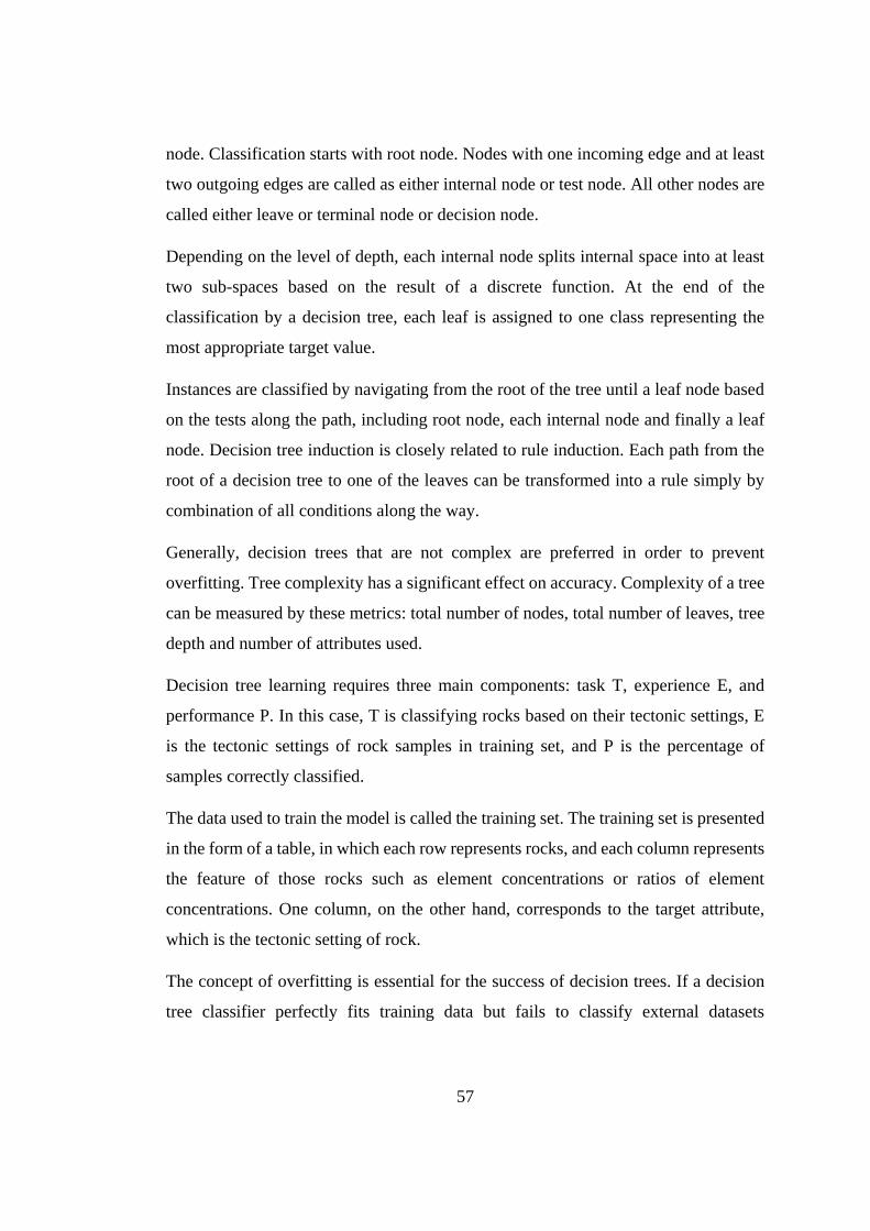
57
node. Classification starts with root node. Nodes with one incoming edge and at least
two outgoing edges are called as either internal node or test node. All other nodes are
called either leave or terminal node or decision node.
Depending on the level of depth, each internal node splits internal space into at least
two sub-spaces based on the result of a discrete function. At the end of the
classification by a decision tree, each leaf is assigned to one class representing the
most appropriate target value.
Instances are classified by navigating from the root of the tree until a leaf node based
on the tests along the path, including root node, each internal node and finally a leaf
node. Decision tree induction is closely related to rule induction. Each path from the
root of a decision tree to one of the leaves can be transformed into a rule simply by
combination of all conditions along the way.
Generally, decision trees that are not complex are preferred in order to prevent
overfitting. Tree complexity has a significant effect on accuracy. Complexity of a tree
can be measured by these metrics: total number of nodes, total number of leaves, tree
depth and number of attributes used.
Decision tree learning requires three main components: task T, experience E, and
performance P. In this case, T is classifying rocks based on their tectonic settings, E
is the tectonic settings of rock samples in training set, and P is the percentage of
samples correctly classified.
The data used to train the model is called the training set. The training set is presented
in the form of a table, in which each row represents rocks, and each column represents
the feature of those rocks such as element concentrations or ratios of element
concentrations. One column, on the other hand, corresponds to the target attribute,
which is the tectonic setting of rock.
The concept of overfitting is essential for the success of decision trees. If a decision
tree classifier perfectly fits training data but fails to classify external datasets
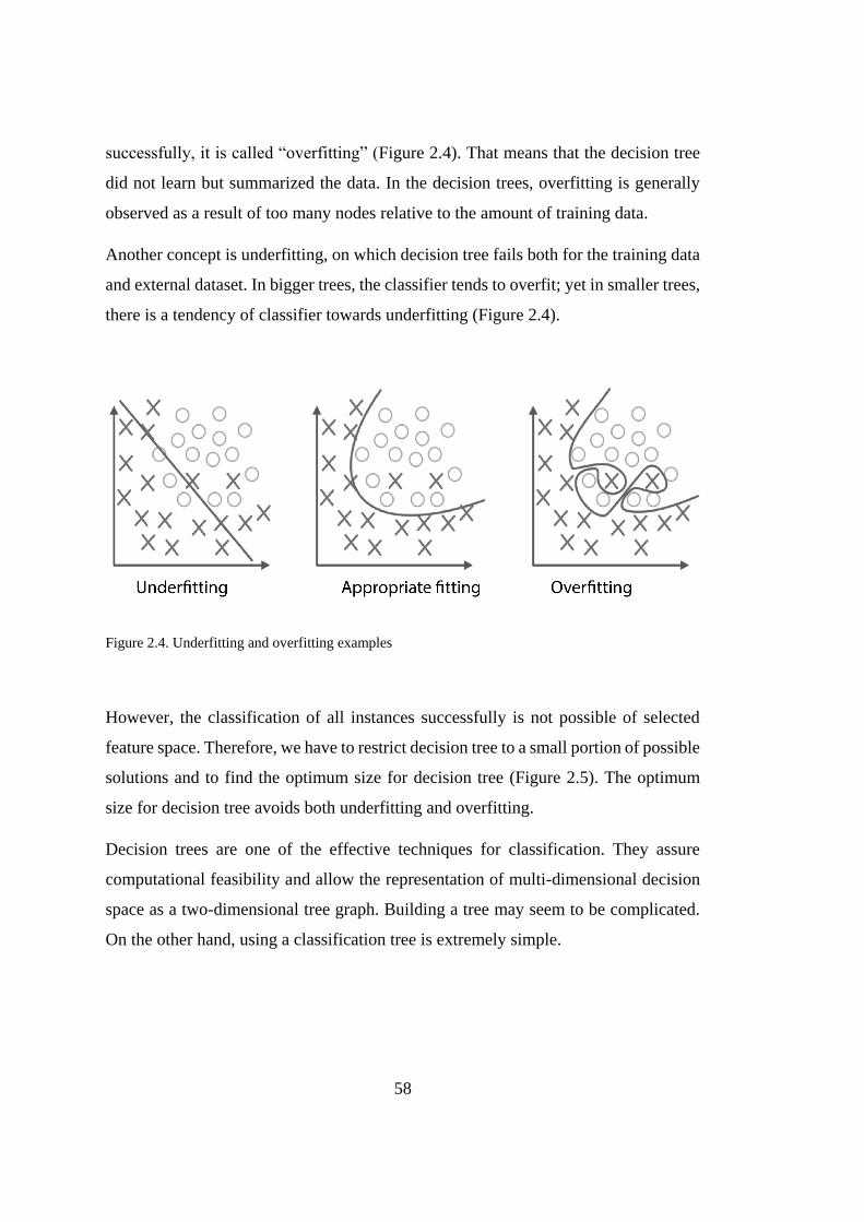
58
successfully, it is called “overfitting” (Figure 2.4). That means that the decision tree
did not learn but summarized the data. In the decision trees, overfitting is generally
observed as a result of too many nodes relative to the amount of training data.
Another concept is underfitting, on which decision tree fails both for the training data
and external dataset. In bigger trees, the classifier tends to overfit; yet in smaller trees,
there is a tendency of classifier towards underfitting (Figure 2.4).
Figure 2.4. Underfitting and overfitting examples
However, the classification of all instances successfully is not possible of selected
feature space. Therefore, we have to restrict decision tree to a small portion of possible
solutions and to find the optimum size for decision tree (Figure 2.5). The optimum
size for decision tree avoids both underfitting and overfitting.
Decision trees are one of the effective techniques for classification. They assure
computational feasibility and allow the representation of multi-dimensional decision
space as a two-dimensional tree graph. Building a tree may seem to be complicated.
On the other hand, using a classification tree is extremely simple.
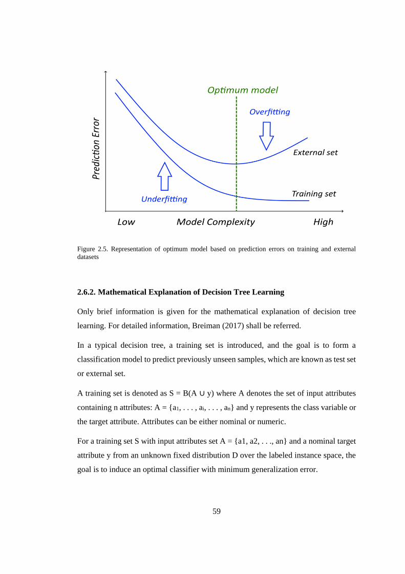
59
Figure 2.5. Representation of optimum model based on prediction errors on training and external
datasets
2.6.2. Mathematical Explanation of Decision Tree Learning
Only brief information is given for the mathematical explanation of decision tree
learning. For detailed information, Breiman (2017) shall be referred.
In a typical decision tree, a training set is introduced, and the goal is to form a
classification model to predict previously unseen samples, which are known as test set
or external set.
A training set is denoted as S = B(A ∪ y) where A denotes the set of input attributes
containing n attributes: A = {a1, . . . , ai, . . . , an} and y represents the class variable or
the target attribute. Attributes can be either nominal or numeric.
For a training set S with input attributes set A = {a1, a2, . . ., an} and a nominal target
attribute y from an unknown fixed distribution D over the labeled instance space, the
goal is to induce an optimal classifier with minimum generalization error.
60
The generalization error is defined as the misclassification rate over the distribution
D, which can be expressed by the equation
𝜀(𝐷𝑇(𝑆), 𝐷) = ∑ 𝐷(𝑥, 𝑦). 𝐿(𝑦, 𝐷𝑇(𝑆)(𝑥))
(𝑥,𝑦)∈𝑈
where L (y, DT(S), D) is the zero one loss function defined with equations
𝐿(𝑦, 𝐷𝑇(𝑆)(𝑥) = {0 𝑖𝑓 𝑦 = 𝐷𝑇(𝑆)(𝑥) 1 𝑖𝑓 𝑦 ≠ 𝐷𝑇(𝑆)(𝑥)
}
The main goal is to induce the best classifier or a set of classifiers that most accurately
classify the members of instance space.
An induction algorithm or simply inducer (also known as learner) is an entity that
obtains a training set and forms a model that generalizes the relationship between the
input attributes and the target attribute and to produce a classifier.
The notation DT represents a decision tree inducer, and DT(S) represents a
classification tree that is induced by performing DT on a training set S. Using DT(S),
it is possible to predict the target value of a tuple xq. This prediction is denoted as
DT(S)(xq).
Suppose we have N data points with J dimensions, which can be expressed as
Xn={𝑥1𝑛,…., 𝑥𝑗
𝑛,…., 𝑥𝐽𝑛} (1 ≤ n ≤ N). All data points belong to one of K classes YN =
c1 | … | ck | … | cK and classification of these data points based on the classes is
expected by using J features. For this case, N represents the number of basic igneous
rock samples, J represents ratios of selected relatively immobile elements, K
represents tectonic settings as classes.
The basic idea behind classification trees is to approximate the parameter space by a
piece size constant function, in other words, to partition X into M disjoint regions
{R1,…..,Rm,…..,RM} (Figure 2.6).
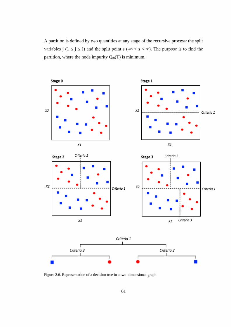
61
A partition is defined by two quantities at any stage of the recursive process: the split
variables j (1 ≤ j ≤ J) and the split point s (-∞ < s < ∞). The purpose is to find the
partition, where the node impurity Qm(T) is minimum.
Figure 2.6. Representation of a decision tree in a two-dimensional graph
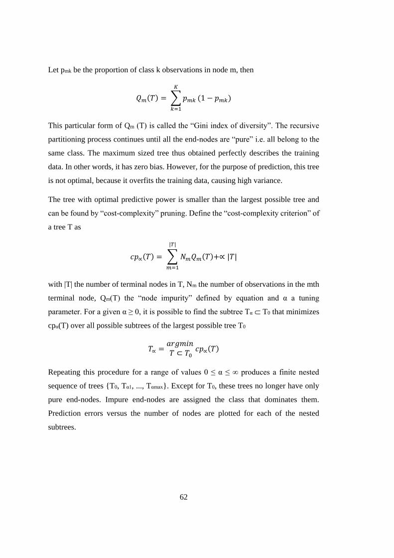
62
Let pmk be the proportion of class k observations in node m, then
𝑄𝑚(𝑇) = ∑ 𝑝𝑚𝑘
𝐾
𝑘=1
(1 − 𝑝𝑚𝑘)
This particular form of Qm (T) is called the “Gini index of diversity”. The recursive
partitioning process continues until all the end-nodes are “pure” i.e. all belong to the
same class. The maximum sized tree thus obtained perfectly describes the training
data. In other words, it has zero bias. However, for the purpose of prediction, this tree
is not optimal, because it overfits the training data, causing high variance.
The tree with optimal predictive power is smaller than the largest possible tree and
can be found by “cost-complexity” pruning. Define the “cost-complexity criterion” of
a tree T as
𝑐𝑝∝(𝑇) = ∑ 𝑁𝑚𝑄𝑚(𝑇)+∝ |𝑇|
|𝑇|
𝑚=1
with |T| the number of terminal nodes in T, Nm the number of observations in the mth
terminal node, Qm(T) the “node impurity” defined by equation and α a tuning
parameter. For a given α ≥ 0, it is possible to find the subtree Tα ⸦ T0 that minimizes
cpα(T) over all possible subtrees of the largest possible tree T0
𝑇∝ =𝑎𝑟𝑔𝑚𝑖𝑛 𝑇 ⊂ 𝑇0
𝑐𝑝∝(𝑇)
Repeating this procedure for a range of values 0 ≤ α ≤ ∞ produces a finite nested
sequence of trees {T0, Tα1, ..., Tαmax}. Except for T0, these trees no longer have only
pure end-nodes. Impure end-nodes are assigned the class that dominates them.
Prediction errors versus the number of nodes are plotted for each of the nested
subtrees.

63
Trees with fewer nodes tend to have a larger bias. The smallest tree with
misclassification error not exceeding minimum misclassification error plus one
standard error is selected as the final decision tree.
2.6.3. Evaluation of Decision Trees
Several indicators are evaluated in order to determine and evaluate the quality of the
decision tree. Evaluation of the decision tree performance is a fundamental aspect of
data science and machine learning. The inducer receives a training set as input data
and constructs a decision tree. Both the decision trees and inducer can be evaluated as
an evaluation criterion.
2.6.3.1. Generalization Error and Classification Accuracy
Let DT(S) be a decision tree for a training set S. The generalization error of DT(S) is
its probability to misclassify an instance selected from instance space.
The classification accuracy of a decision tree is one minus the generalization error,
and is the primary evaluation criteria for decision trees.
The training error is defined as the percentage of correctly classified samples in the
training set. The training error can also be used instead of the classification accuracy,
but it can result in bias especially with an inducer with a risk of overfitting.
2.6.3.2. Alternatives for Accuracy Measurement
Precision is an alternative to measure the performance of decision tree. Precision
measures the number of positive samples also classified as positive by decision tree.
Precision = (True positive) / (True positive + False positive)
Another parameter is sensitivity (which is also known as recall), which is the ratio of
true positives to the total number of positives.
Sensitivity = True positive / Positive
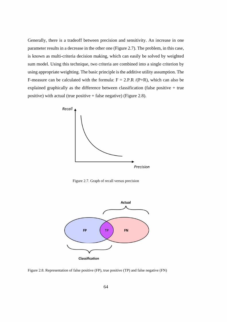
64
Generally, there is a tradeoff between precision and sensitivity. An increase in one
parameter results in a decrease in the other one (Figure 2.7). The problem, in this case,
is known as multi-criteria decision making, which can easily be solved by weighted
sum model. Using this technique, two criteria are combined into a single criterion by
using appropriate weighting. The basic principle is the additive utility assumption. The
F-measure can be calculated with the formula: F = 2.P.R /(P+R), which can also be
explained graphically as the difference between classification (false positive + true
positive) with actual (true positive + false negative) (Figure 2.8).
Figure 2.7. Graph of recall versus precision
Figure 2.8. Representation of false positive (FP), true positive (TP) and false negative (FN)
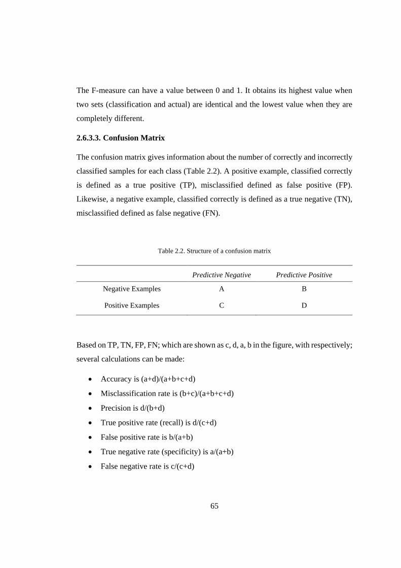
65
The F-measure can have a value between 0 and 1. It obtains its highest value when
two sets (classification and actual) are identical and the lowest value when they are
completely different.
2.6.3.3. Confusion Matrix
The confusion matrix gives information about the number of correctly and incorrectly
classified samples for each class (Table 2.2). A positive example, classified correctly
is defined as a true positive (TP), misclassified defined as false positive (FP).
Likewise, a negative example, classified correctly is defined as a true negative (TN),
misclassified defined as false negative (FN).
Table 2.2. Structure of a confusion matrix
Predictive Negative Predictive Positive
Negative Examples A B
Positive Examples C D
Based on TP, TN, FP, FN; which are shown as c, d, a, b in the figure, with respectively;
several calculations can be made:
Accuracy is (a+d)/(a+b+c+d)
Misclassification rate is (b+c)/(a+b+c+d)
Precision is d/(b+d)
True positive rate (recall) is d/(c+d)
False positive rate is b/(a+b)
True negative rate (specificity) is a/(a+b)
False negative rate is c/(c+d)
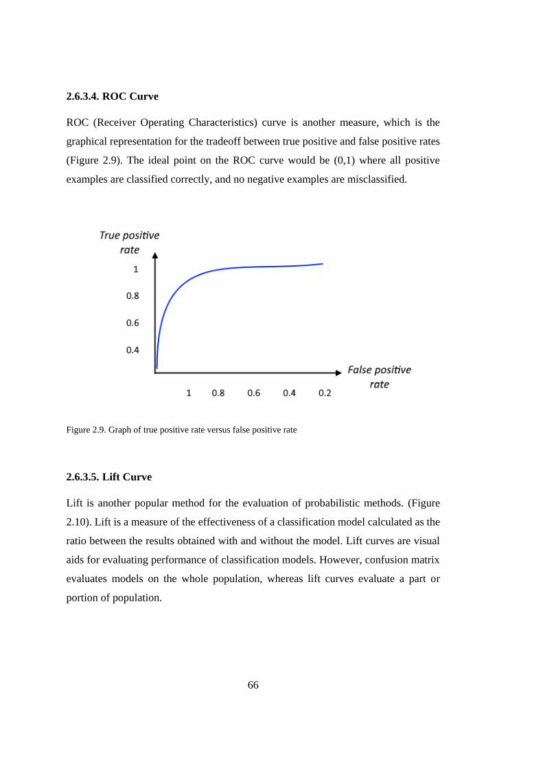
66
2.6.3.4. ROC Curve
ROC (Receiver Operating Characteristics) curve is another measure, which is the
graphical representation for the tradeoff between true positive and false positive rates
(Figure 2.9). The ideal point on the ROC curve would be (0,1) where all positive
examples are classified correctly, and no negative examples are misclassified.
Figure 2.9. Graph of true positive rate versus false positive rate
2.6.3.5. Lift Curve
Lift is another popular method for the evaluation of probabilistic methods. (Figure
2.10). Lift is a measure of the effectiveness of a classification model calculated as the
ratio between the results obtained with and without the model. Lift curves are visual
aids for evaluating performance of classification models. However, confusion matrix
evaluates models on the whole population, whereas lift curves evaluate a part or
portion of population.
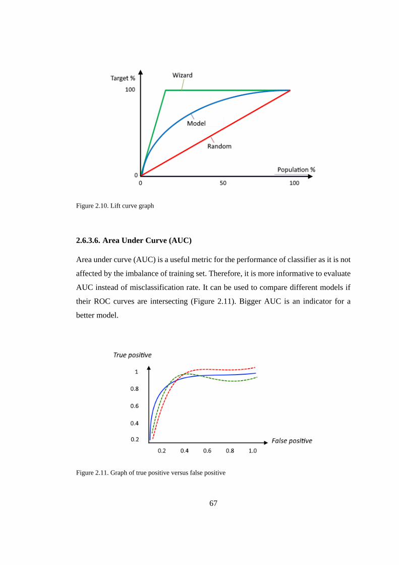
67
Figure 2.10. Lift curve graph
2.6.3.6. Area Under Curve (AUC)
Area under curve (AUC) is a useful metric for the performance of classifier as it is not
affected by the imbalance of training set. Therefore, it is more informative to evaluate
AUC instead of misclassification rate. It can be used to compare different models if
their ROC curves are intersecting (Figure 2.11). Bigger AUC is an indicator for a
better model.
Figure 2.11. Graph of true positive versus false positive

68
2.6.4. Splitting Decision Trees
Decision tree induces generally split decision trees using univariate discrete splitting
functions. In other words, an internal node is split according to the value of a single
attribute.
2.6.4.1. Impurity-based criteria
Given a random variable x with k discrete values, distributed according to P = (p1, p2,
. . ., pk), an impurity measure is a function φ: [0, 1] k → R that satisfies the following
conditions:
• φ (P)≥0.
• φ (P) is minimum if ∃i such that component pi = 1.
• φ (P) is maximum if ∀i, 1 ≤ i ≤ k, pi = 1/k.
• φ (P) is symmetric with respect to components of P.
• φ (P) is smooth (differentiable everywhere) in its range
It should be noted that if the probability vector has a component of 1 (the variable x
gets only one value), then the variable is defined as pure. On the other hand, if all
components are equal the level of impurity reaches the maximum.
Given a training set S the probability vector of the target attribute y is defined as:
𝑃𝑦(𝑆) = (|𝜎𝑦=𝑐1 = 𝑆|
|𝑆|, … ,
|𝜎𝑦=𝑐|𝑑𝑜𝑚(𝑦)| = 𝑆|
|𝑆|)
2.6.4.2. Information Gain
Information Gain is an impurity-based criterion that uses the entropy measure
(originating from information theory) as the impurity measure.

69
Information gain is closely related to the maximum likelihood estimation (MLE),
which is a popular statistical method used to make inferences about parameters of the
underlying probability distribution from a given dataset.
2.6.4.3. Gini Index
The Gini index is an impurity-based criterion that measures the divergences between
the probability distributions of the target attributes values.
2.6.4.4. Gain Ratio
The gain ratio normalizes the information gain with this equation:
𝐺𝑎𝑖𝑛 𝑅𝑎𝑡𝑖𝑜(𝑎𝑖 , 𝑆) = 𝐼𝑛𝑓𝑜𝑟𝑚𝑎𝑡𝑖𝑜𝑛 𝐺𝑎𝑖𝑛(𝑎𝑖 , 𝑆)
𝐸𝑛𝑡𝑟𝑜𝑝𝑦(𝑎𝑖 , 𝑆)
The information gain is calculated for all attributes. As a consequence of considering
only attributes that have performed at least as well as the average information gain,
the attribute that has obtained the best ratio gain is selected. Quinlan (1988) has shown
that the gain ratio tends to outperform simple information gain criteria, both in
accuracy and in terms of classifier complexity. A penalty is assessed for the
information gain of a continuous attribute with many potential splits.
2.6.5. Stopping Decision Trees
A decision tree is grown until a stopping criterion is provided. The following
conditions are generally accepted and applied as effective stopping criteria:
1. All instances in each leaf of the training set are correctly classified (belonging
to the same class)
2. The maximum tree depth is reached.
3. The number of cases in the terminal node is less than the minimum number of
cases for parent nodes.
4. If nodes are split, the number of cases in one or more child nodes would be
less than the minimum number of cases for child nodes.

70
5. The best splitting criterion is not greater than a certain threshold.
2.6.6. Pruning Decision Trees
If a constructed decision tree results in overfitting, then the pruning of decision tree is
applied, and the common method is cost-complexity pruning.
Cost complexity pruning (also known as weakest link pruning or error complexity
pruning) proceeds in two stages (Breiman, 2017). In the first stage, a sequence of trees
T0, T1, . . ., Tk is built on the training data where T0 is the original tree before pruning
and Tk is the root tree. In the second stage, one of these trees is chosen as the pruned
tree, based on its generalization error estimation. The tree Ti+1 is obtained by
replacing one or more of the sub-trees in the predecessor tree Ti with suitable leaves.
The sub-trees that are pruned are those that obtain the lowest increase in the apparent
error rate per pruned leaf:
𝛼 =𝜀(𝑝𝑟𝑢𝑛𝑒𝑑(𝑇, 𝑡), 𝑆) − 𝜀(𝑇, 𝑆)
|𝑙𝑒𝑎𝑣𝑒𝑠(𝑇)| − |𝑙𝑒𝑎𝑣𝑒𝑠(𝑝𝑟𝑢𝑛𝑒𝑑(𝑇, 𝑡))|
where ε (T, S) indicates the error rate of the tree T over the sample S and |leaves (T)|
denotes the number of leaves in T. Pruned (T, t) denotes the tree obtained by replacing
the node t in T with a suitable leaf. In the second phase, the generalization error of
each pruned tree is estimated. The best pruned tree is then selected. If the given dataset
is large enough, the authors suggest breaking it into a training set and a pruning set.
The trees are constructed using the training set and evaluated on the pruning set. On
the other hand, if the given dataset is not large enough, they propose using cross-
validation methodology, despite the computational complexity implications.
2.6.7. Advantages and Disadvantages of Decision Trees
The main advantages of decision trees can be listed as:
1. They are self-explanatory and easy to follow. A decision tree can be easily
understood and followed by non-professional user.
2. They can handle both nominal and numeric input attributes.

71
3. Their representation is rich.
4. They can handle datasets with errors and missing data.
5. Decision trees are considered to be non-parametric. In other words, they do
not include any assumptions about the spatial distribution or about classifier
structure.
6. Decision trees are simple as they only require to follow conditions along a
single path from the root to the leaf.
On the other hand, the disadvantages of a decision tree can be listed as:
1. They mostly require that the target attribute to have only discrete values.
2. They show low performance when complex interactions are present.
3. They are over-sensitive to irrelevant attributes or to noises making decision
trees unstable. A minor change in one split may change everything from that
split to the leaf nodes.
4. Missing data and errors can be handled, but extreme effort and attention are
required.
2.6.8. Application of Decision Tree Learning to Tectono-Magmatic
Discrimination
Tectono-magmatic discrimination methods for mafic igneous rocks are constructed
and suggested by using the Decision Tree Method in Orange (a free Data Mining
software) based on tectonic settings as classes and ratios of relatively immobile
elements as features. The database is divided into three groups: Training dataset, test
dataset, and external dataset. The training dataset is used to construct the tectono-
magmatic discrimination methods. The test dataset is used to run an initial control for
the quality of constructed trees. External datasets are used to check the external
applicability of constructed trees in varying conditions (such as geographical location,
geological setting, geochemical characteristics, geological age, alteration etc).
Multiple decision trees are constructed for the tectono-magmatic discrimination of
basic and ultrabasic igneous rocks (Figure 2.12). First, subduction-related settings are

72
discriminated from non-subduction-related settings. Subduction settings are
continental arcs, oceanic arcs, and oceanic back-arcs, whereas non-subduction settings
are continental within-plates, mid-oceanic ridges, oceanic islands and oceanic
plateaus.
Three alternative decision trees are constructed for tectono-magmatic discrimination
between subduction settings and non-subduction settings. The first decision tree
involves only ratios of relatively immobile elements and has only one branch. The
second decision tree is a multi-branched decision tree that involves ratios of relatively
immobile elements and also Nb/Nb* ratio. Element ratios using TiO2 are eliminated
for the third decision tree to propose an alternative decision tree.
As the first alternative of tectono-magmatic discrimination between subduction and
non-subduction settings, a decision stump is constructed.
Out of 2.642 samples (training and test set), 2.114 samples are used to construct the
decision tree, and 528 samples are used to test the decision tree.
Selected features are only element ratios of selected immobile elements (Th, La, Nb,
Y, Yb, Zr, Hf, Sm, Nd, TiO2). Absolute values of immobile elements are only used
for calculation of element ratios and then ignored in the construction of decision trees.
Out of selected element ratios (Th/Nb, La/Nb, Th/La, Zr/Hf, Zr/Nb, La/Y, La/Yb,
Nb/Y, Nb/Yb, Sm/Y, Sm/Yb, Nd/Zr, La/Sm, Sm/Hf, Y/Yb, Zr/Sm, Zr/Y, Zr/Yb,
Th/Y, Th/Yb, Sm/Nb, Sm/Nd, Zr/TiO2, TiO2/Y, TiO2/Yb, Nd/TiO2, Nb/TiO2), Th/Nb
is the feature with highest information gain (0.528), gain ratio (0.264), and gini index
(0.276) (Table 2.3) for the tectono-magmatic discrimination between subduction and
non-subduction settings.
As the second alternative of tectono-magmatic discrimination between subduction and
non-subduction settings, a multi-branched decision tree is constructed.
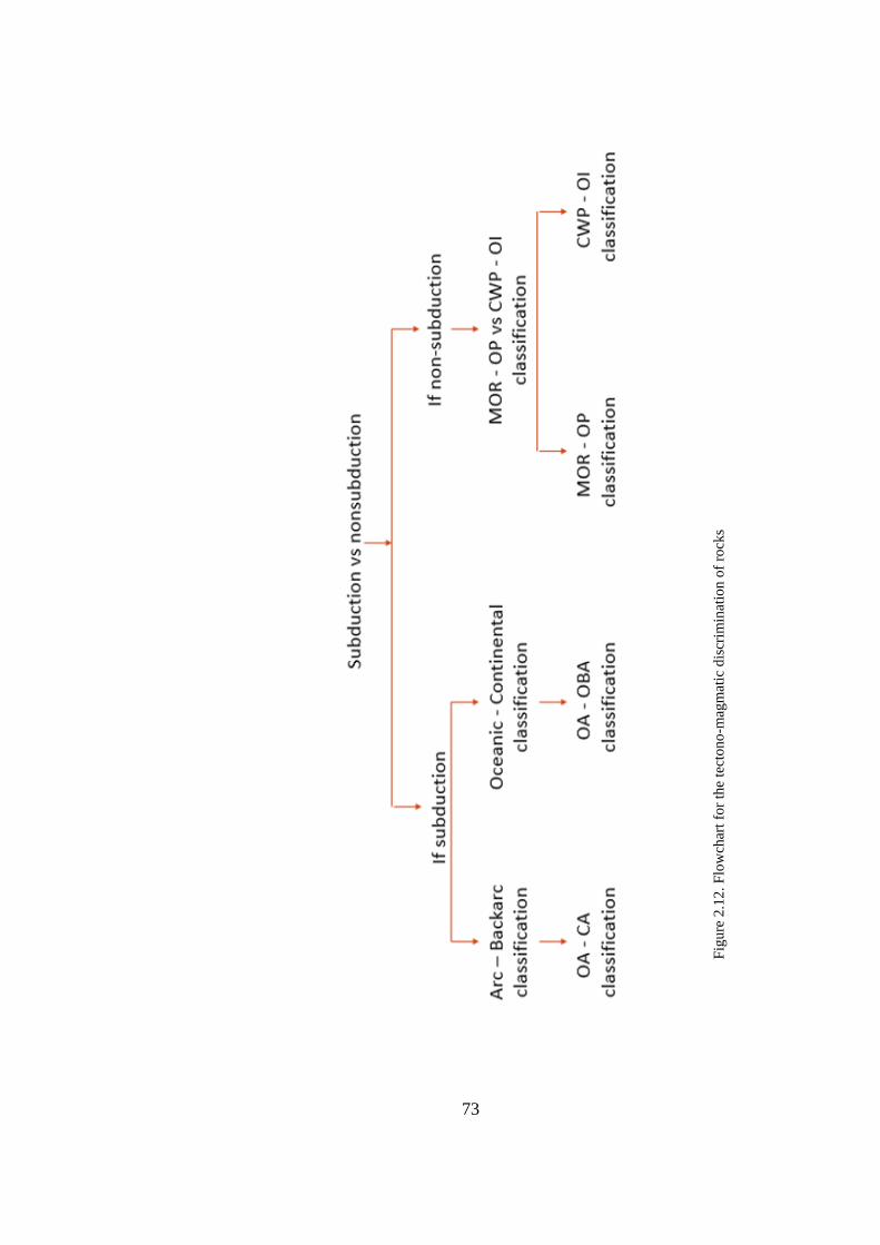
73
Figure 2.12. Flowchart for the tectono-magmatic discrimination of rocks
Fig
ure
2.1
2. F
low
char
t fo
r th
e te
cto
no
-mag
mat
ic d
iscr
imin
atio
n o
f ro
cks
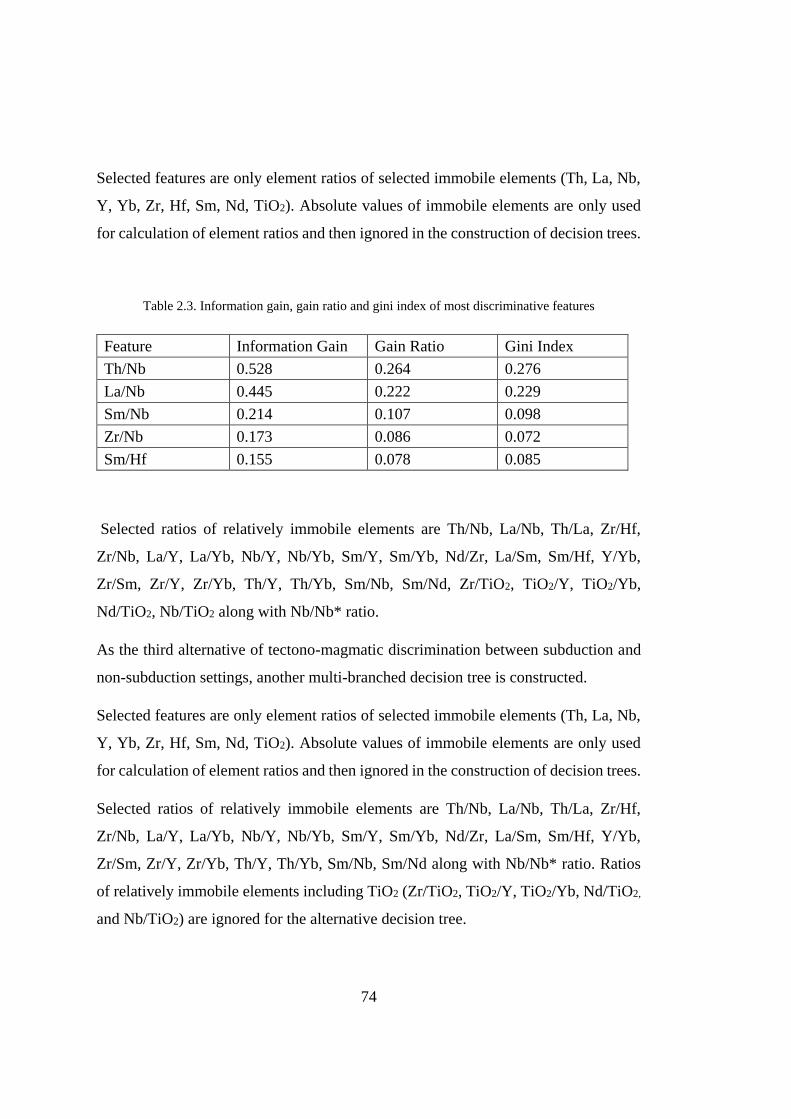
74
Selected features are only element ratios of selected immobile elements (Th, La, Nb,
Y, Yb, Zr, Hf, Sm, Nd, TiO2). Absolute values of immobile elements are only used
for calculation of element ratios and then ignored in the construction of decision trees.
Table 2.3. Information gain, gain ratio and gini index of most discriminative features
Feature Information Gain Gain Ratio Gini Index
Th/Nb 0.528 0.264 0.276
La/Nb 0.445 0.222 0.229
Sm/Nb 0.214 0.107 0.098
Zr/Nb 0.173 0.086 0.072
Sm/Hf 0.155 0.078 0.085
Selected ratios of relatively immobile elements are Th/Nb, La/Nb, Th/La, Zr/Hf,
Zr/Nb, La/Y, La/Yb, Nb/Y, Nb/Yb, Sm/Y, Sm/Yb, Nd/Zr, La/Sm, Sm/Hf, Y/Yb,
Zr/Sm, Zr/Y, Zr/Yb, Th/Y, Th/Yb, Sm/Nb, Sm/Nd, Zr/TiO2, TiO2/Y, TiO2/Yb,
Nd/TiO2, Nb/TiO2 along with Nb/Nb* ratio.
As the third alternative of tectono-magmatic discrimination between subduction and
non-subduction settings, another multi-branched decision tree is constructed.
Selected features are only element ratios of selected immobile elements (Th, La, Nb,
Y, Yb, Zr, Hf, Sm, Nd, TiO2). Absolute values of immobile elements are only used
for calculation of element ratios and then ignored in the construction of decision trees.
Selected ratios of relatively immobile elements are Th/Nb, La/Nb, Th/La, Zr/Hf,
Zr/Nb, La/Y, La/Yb, Nb/Y, Nb/Yb, Sm/Y, Sm/Yb, Nd/Zr, La/Sm, Sm/Hf, Y/Yb,
Zr/Sm, Zr/Y, Zr/Yb, Th/Y, Th/Yb, Sm/Nb, Sm/Nd along with Nb/Nb* ratio. Ratios
of relatively immobile elements including TiO2 (Zr/TiO2, TiO2/Y, TiO2/Yb, Nd/TiO2,
and Nb/TiO2) are ignored for the alternative decision tree.
75
If this classification returns with a result of subduction-related settings, then one of
two approaches would be selected.
At the first approach, the arc-related settings are discriminated from the back-arc
setting and then arc-related settings are discriminated from each other.
For discrimination of arc and back-arc settings, out of 668 samples (training and test
set), 535 samples are used to construct the decision tree, and 133 samples are used to
test decision tree. Later, for discrimination of oceanic arc from continental arc settings
within arc-related samples, out of 562 samples (training and test set), 450 samples are
used to construct decision tree, and 112 samples are used to test decision tree.
At the second approach, oceanic settings are discriminated from continental settings,
and then oceanic settings are discriminated from each other.
For the discrimination of oceanic and continental settings, out of 668 samples (training
and test set), 535 samples are used to construct the decision tree, and 133 samples are
used to test the decision tree. Later, for discrimination of oceanic arc from oceanic
back-arc settings within samples of oceanic setting, out of 487 samples (training and
test set), 390 samples are used to construct decision tree, and 97 samples are used to
test decision tree.
If the classification returns with a result of non-subduction-related settings, then first
mid-oceanic ridges and oceanic plateaus are discriminated from continental within-
plates and oceanic islands.
If non-subduction-related setting is either mid-oceanic ridge or oceanic plateau, then
these are discriminated from each other. If it is either continental within-plate or
oceanic island, then these are discriminated from each other.
For the discrimination of non-subduction-related settings into two parts as mid-
oceanic ridge and oceanic plateau as first part and continental within-plates and
oceanic islands as second part, out of 1.974 samples (training and test set), 1.580
samples are used to construct decision tree, and 394 samples are used to test decision

76
tree. Later, for discrimination of mid-oceanic ridges from oceanic plateaus within the
first part, out of 1.120 samples (training and test set), 896 samples are used to construct
decision tree, and 224 samples are used to test decision tree. For discrimination of
continental within-plates from oceanic islands within the second part, out of 854
samples (training and test set), 684 samples are used to construct decision tree, and
170 samples are used to test decision tree.
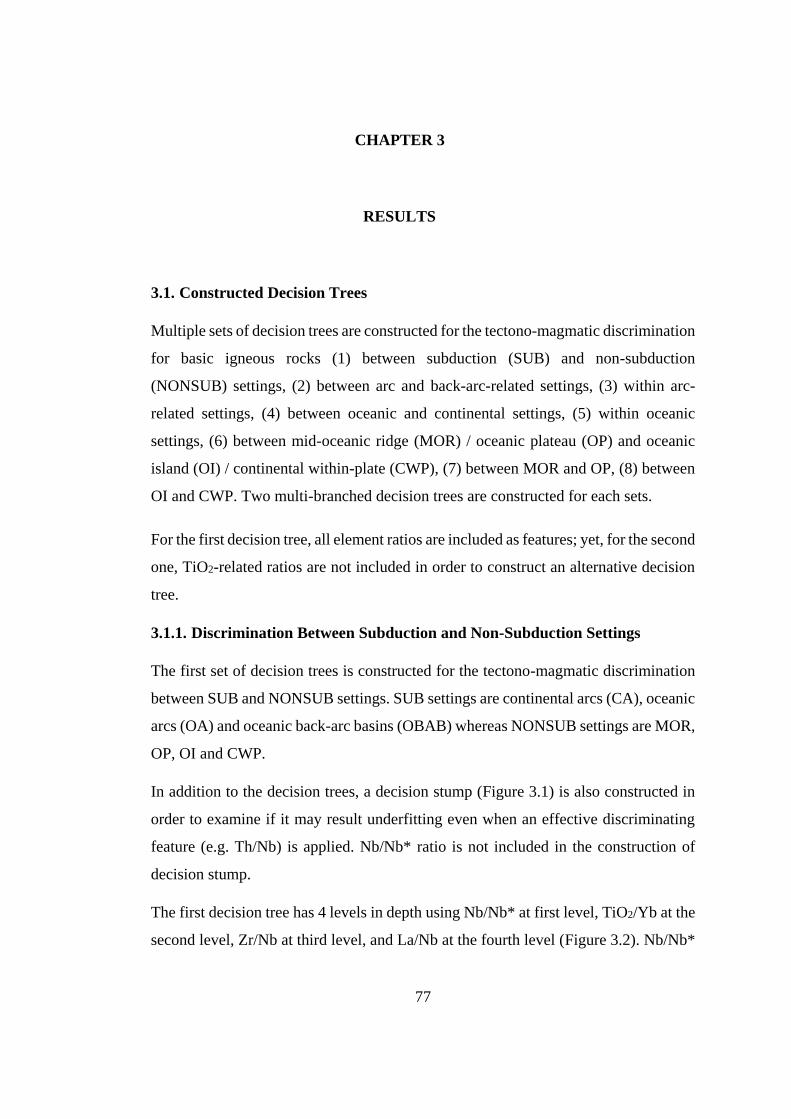
77
CHAPTER 3
3. RESULTS
3.1. Constructed Decision Trees
Multiple sets of decision trees are constructed for the tectono-magmatic discrimination
for basic igneous rocks (1) between subduction (SUB) and non-subduction
(NONSUB) settings, (2) between arc and back-arc-related settings, (3) within arc-
related settings, (4) between oceanic and continental settings, (5) within oceanic
settings, (6) between mid-oceanic ridge (MOR) / oceanic plateau (OP) and oceanic
island (OI) / continental within-plate (CWP), (7) between MOR and OP, (8) between
OI and CWP. Two multi-branched decision trees are constructed for each sets.
For the first decision tree, all element ratios are included as features; yet, for the second
one, TiO2-related ratios are not included in order to construct an alternative decision
tree.
3.1.1. Discrimination Between Subduction and Non-Subduction Settings
The first set of decision trees is constructed for the tectono-magmatic discrimination
between SUB and NONSUB settings. SUB settings are continental arcs (CA), oceanic
arcs (OA) and oceanic back-arc basins (OBAB) whereas NONSUB settings are MOR,
OP, OI and CWP.
In addition to the decision trees, a decision stump (Figure 3.1) is also constructed in
order to examine if it may result underfitting even when an effective discriminating
feature (e.g. Th/Nb) is applied. Nb/Nb* ratio is not included in the construction of
decision stump.
The first decision tree has 4 levels in depth using Nb/Nb* at first level, TiO2/Yb at the
second level, Zr/Nb at third level, and La/Nb at the fourth level (Figure 3.2). Nb/Nb*
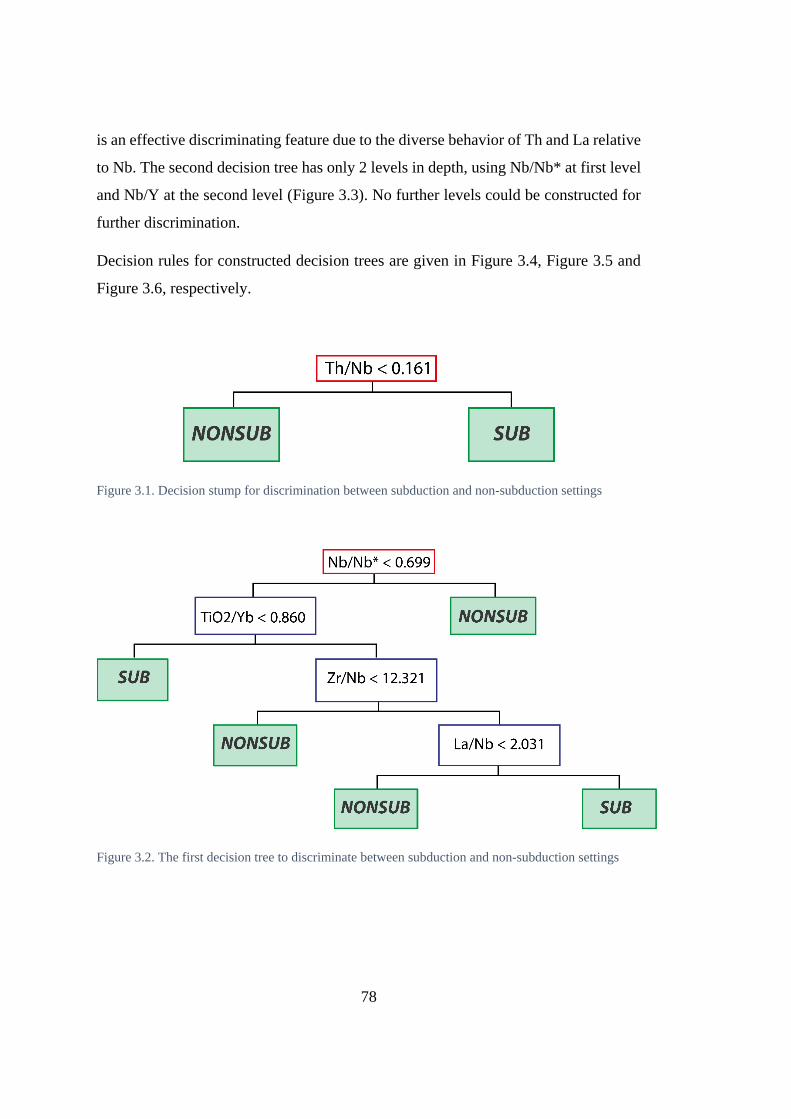
78
is an effective discriminating feature due to the diverse behavior of Th and La relative
to Nb. The second decision tree has only 2 levels in depth, using Nb/Nb* at first level
and Nb/Y at the second level (Figure 3.3). No further levels could be constructed for
further discrimination.
Decision rules for constructed decision trees are given in Figure 3.4, Figure 3.5 and
Figure 3.6, respectively.
Figure 3.1. Decision stump for discrimination between subduction and non-subduction settings
Figure 3.2. The first decision tree to discriminate between subduction and non-subduction settings
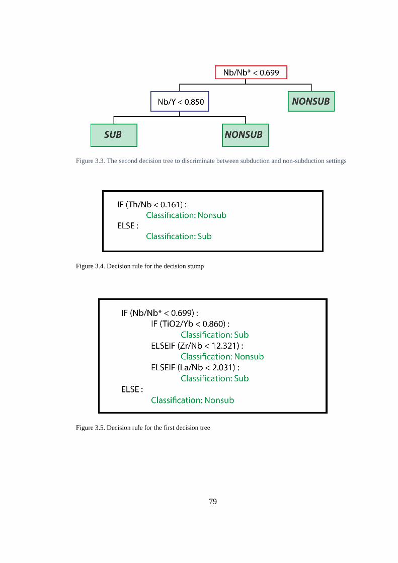
79
Figure 3.3. The second decision tree to discriminate between subduction and non-subduction settings
Figure 3.4. Decision rule for the decision stump
Figure 3.5. Decision rule for the first decision tree
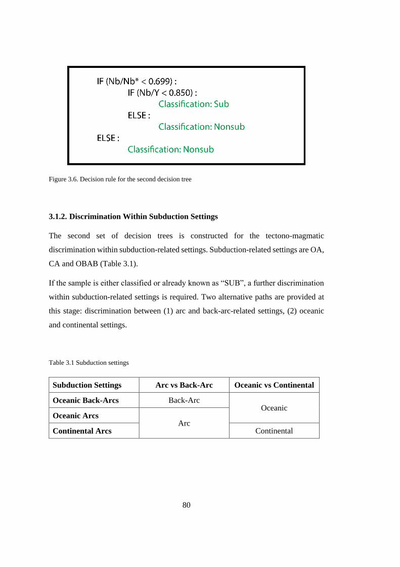
80
Figure 3.6. Decision rule for the second decision tree
3.1.2. Discrimination Within Subduction Settings
The second set of decision trees is constructed for the tectono-magmatic
discrimination within subduction-related settings. Subduction-related settings are OA,
CA and OBAB (Table 3.1).
If the sample is either classified or already known as “SUB”, a further discrimination
within subduction-related settings is required. Two alternative paths are provided at
this stage: discrimination between (1) arc and back-arc-related settings, (2) oceanic
and continental settings.
Table 3.1 Subduction settings
Subduction Settings Arc vs Back-Arc Oceanic vs Continental
Oceanic Back-Arcs Back-Arc Oceanic
Oceanic Arcs Arc
Continental Arcs Continental

81
3.1.2.1. The First Path for Discrimination Within Subduction Settings
The first path involves two-stage discrimination within subduction settings: (1)
between arc and back-arc-related settings, (2) within arc-related settings.
3.1.2.1.1. Discrimination Between Arc and Back-Arc-Related Settings
Two decision trees are constructed for the tectono-magmatic discrimination between
arc and back-arc-related settings. Both decision trees have 5 levels of depth. The first
decision tree (Figure 3.7) use Nb/Nb* at first level, Nd/Zr at the second level, TiO2/Y,
and Nd/TiO2 at the third level, Y/Yb at fourth level and Zr/Hf at fifth level. The second
decision tree (Figure 3.8), on the other hand, use Nb/Nb* at first level, Nd/Zr at second
level, Zr/Hf and Zr/Nb at third level, Zr/Y and Y/Yb at fourth level and Nd/Zr and
Zr/Hf at fifth level.
Figure 3.7. The first decision tree to discriminate between arc and back-arc-related settings
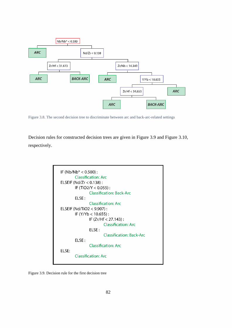
82
Figure 3.8. The second decision tree to discriminate between arc and back-arc-related settings
Decision rules for constructed decision trees are given in Figure 3.9 and Figure 3.10,
respectively.
Figure 3.9. Decision rule for the first decision tree
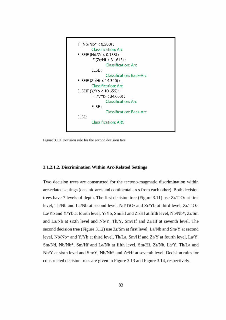
83
Figure 3.10. Decision rule for the second decision tree
3.1.2.1.2. Discrimination Within Arc-Related Settings
Two decision trees are constructed for the tectono-magmatic discrimination within
arc-related settings (oceanic arcs and continental arcs from each other). Both decision
trees have 7 levels of depth. The first decision tree (Figure 3.11) use Zr/TiO2 at first
level, Th/Nb and La/Nb at second level, Nd/TiO2 and Zr/Yb at third level, Zr/TiO2,
La/Yb and Y/Yb at fourth level, Y/Yb, Sm/Hf and Zr/Hf at fifth level, Nb/Nb*, Zr/Sm
and La/Nb at sixth level and Nb/Y, Th/Y, Sm/Hf and Zr/Hf at seventh level. The
second decision tree (Figure 3.12) use Zr/Sm at first level, La/Nb and Sm/Y at second
level, Nb/Nb* and Y/Yb at third level, Th/La, Sm/Hf and Zr/Y at fourth level, La/Y,
Sm/Nd, Nb/Nb*, Sm/Hf and La/Nb at fifth level, Sm/Hf, Zr/Nb, La/Y, Th/La and
Nb/Y at sixth level and Sm/Y, Nb/Nb* and Zr/Hf at seventh level. Decision rules for
constructed decision trees are given in Figure 3.13 and Figure 3.14, respectively.
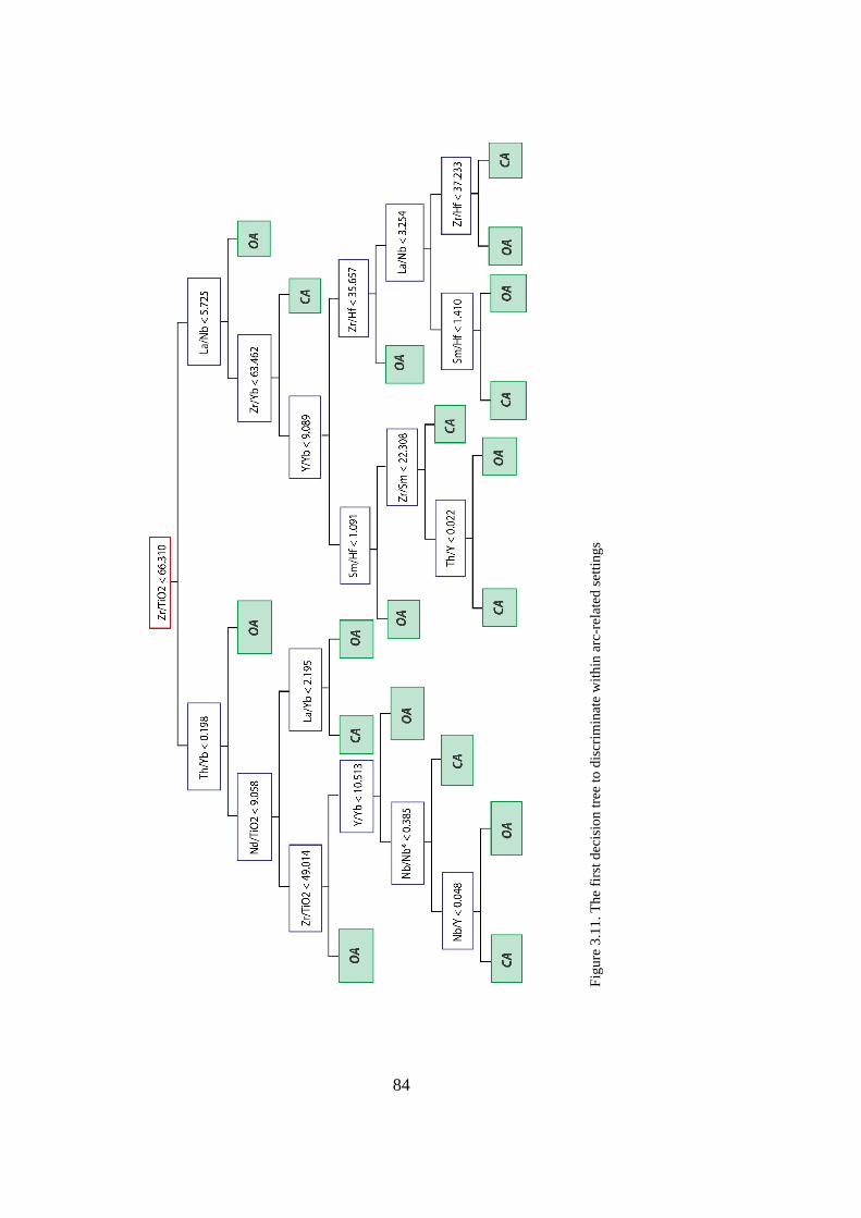
84
Figure 3.11. The first decision tree to discriminate within arc-related settings
Fig
ure
3.1
1.
The
firs
t dec
isio
n t
ree
to d
iscr
imin
ate
wit
hin
arc
-rel
ated
set
tin
gs
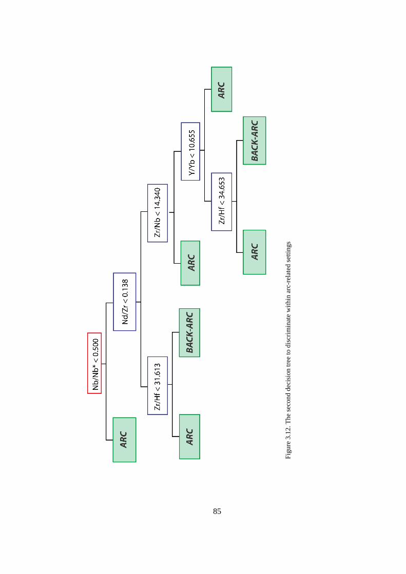
85
Figure 3.12. The second decision tree to discriminate within arc-related settings
Fig
ure
3.1
2.
The
seco
nd
dec
isio
n t
ree
to d
iscr
imin
ate
wit
hin
arc
-rel
ated
set
tin
gs
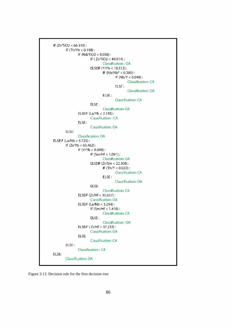
86
Figure 3.13. Decision rule for the first decision tree
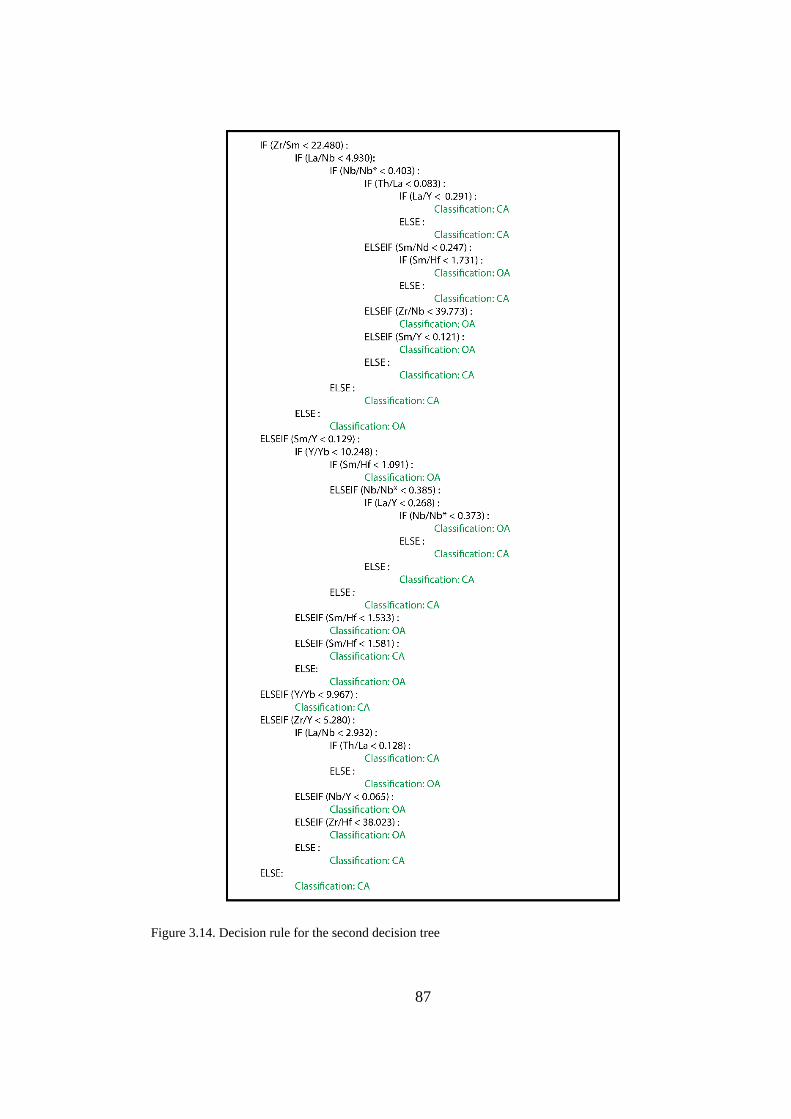
87
Figure 3.14. Decision rule for the second decision tree
88
3.1.2.2. The Second Path for Discrimination Within Subduction Settings
The second path involves two-stage discrimination within subduction settings: (1)
between oceanic and continental settings, (2) within oceanic settings.
3.1.2.2.1. Discrimination Between Oceanic and Continental Settings
Two decision trees are constructed for the tectono-magmatic discrimination between
oceanic and continental settings. Both decision trees have 7 levels of depth. The first
decision tree (Figure 3.15) use Sm/Yb at first level, Nd/Zr at second level, Th/Nb and
Y/Yb at third level, Zr/TiO2, La/Nb, Nb/Nb* and La/Sm at fourth level, La/Nb, Nd/Zr
and Nb/Yb at fifth level, TiO2/Y, Nb/Nb* and Th/Nb at sixth level and Zr/Hf and
Th/La at seventh level. The second decision tree (Figure 3.16) use Sm/Yb at first level,
Nd/Zr at second level, Th/Nb and Y/Yb at third level, Th/La, La/Nb, Nb/Nb* and
La/Sm at fourth level, Sm/Hf, Nd/Zr and Nb/Yb at fifth level, La/Nb, Nb/Nb* and
Th/Nb at sixth level and Nb/Y, Zr/Hf and Th/La at seventh level. Decision rules for
constructed decision trees are given in Figure 3.17 and Figure 3.18, respectively.
3.1.2.2.2. Discrimination Within Oceanic Settings
Two decision trees are constructed for the tectono-magmatic discrimination within
oceanic settings (oceanic arcs and oceanic back-arc basins from each other). Both
decision trees have 6 levels of depth. The first decision tree (Figure 3.19) use Th/Nb
at first level, Sm/Yb and Zr/Hf at second level, La/Nb and Th/Nb at third level,
Nb/Nb*, Nd/Zr and TiO2/Yb at fourth level, Nb/Nb* and Zr/Hf at fifth level and Y/Yb
and Nb/Yb at sixth level. The second decision tree (Figure 3.20) use Th/Nb at first
level, Sm/Yb and Zr/Hf at second level, La/Nb and Th/Nb at third level, Nb/Nb*,
Nd/Zr and La/Sm at fourth level, Nb/Nb* and Sm/Y at fifth level and Y/Yb at sixth
level. Decision rules for constructed decision trees are given in Figure 3.21 and Figure
3.22, respectively.
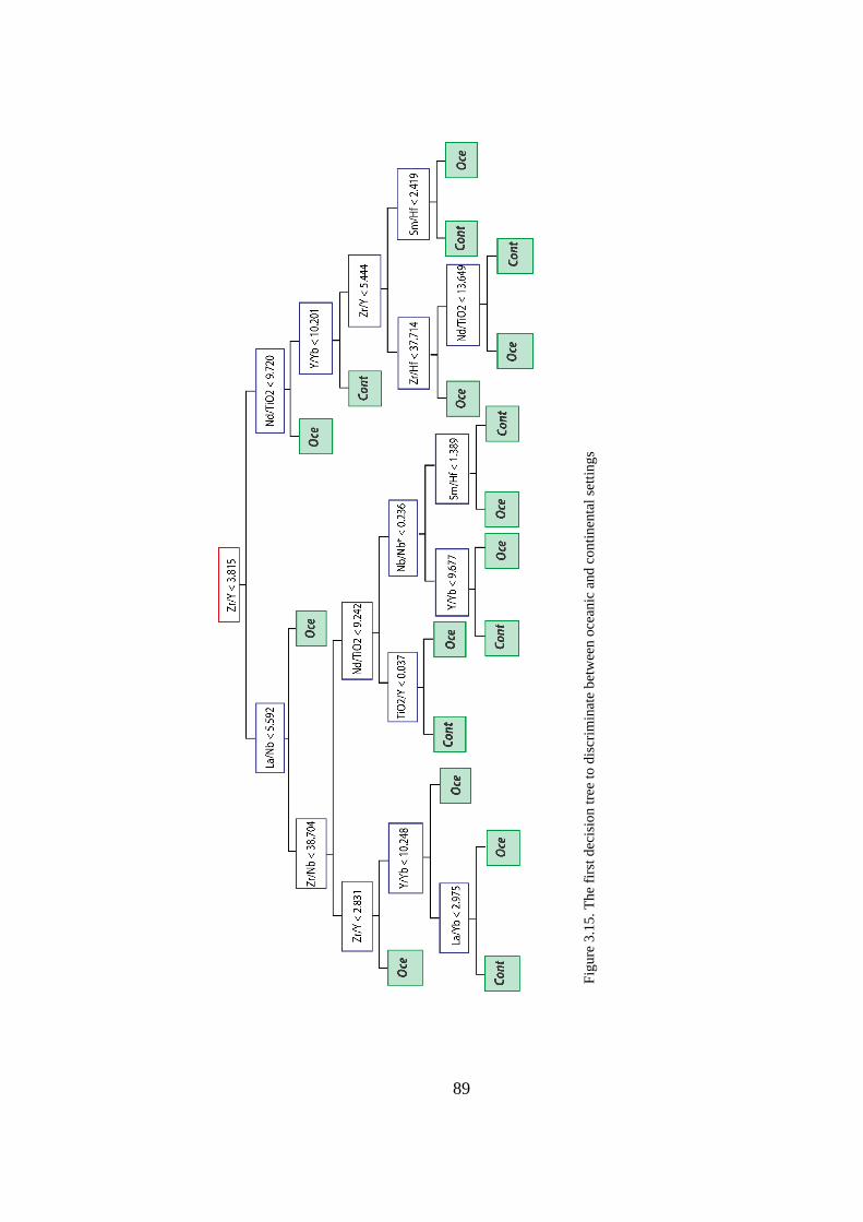
89
Figure 3.15. The first decision tree to discriminate between oceanic and continental settings
Fig
ure
3.1
5.
The
firs
t dec
isio
n t
ree
to d
iscr
imin
ate
bet
wee
n o
cean
ic a
nd
co
nti
nen
tal
sett
ing
s
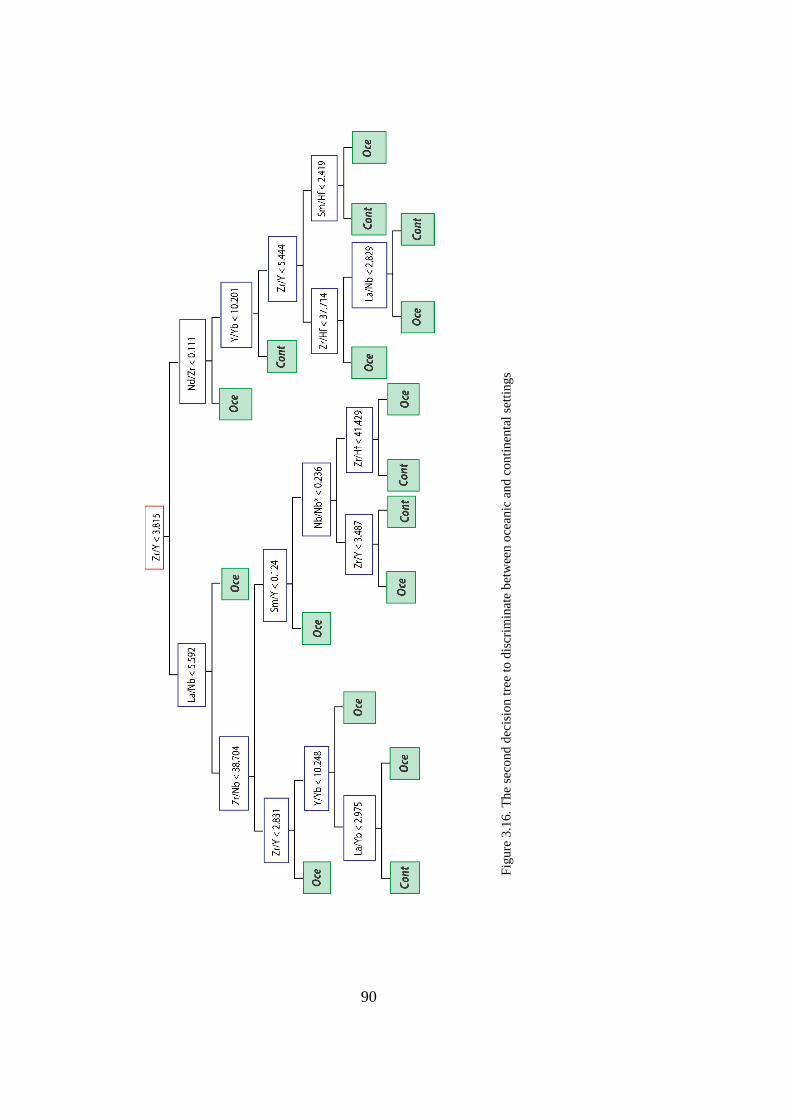
90
Figure 3.16. The second decision tree to discriminate between oceanic and continental settings
Fig
ure
3.1
6.
The
seco
nd
dec
isio
n t
ree
to d
iscr
imin
ate
bet
wee
n o
cean
ic a
nd
co
nti
nen
tal
sett
ing
s
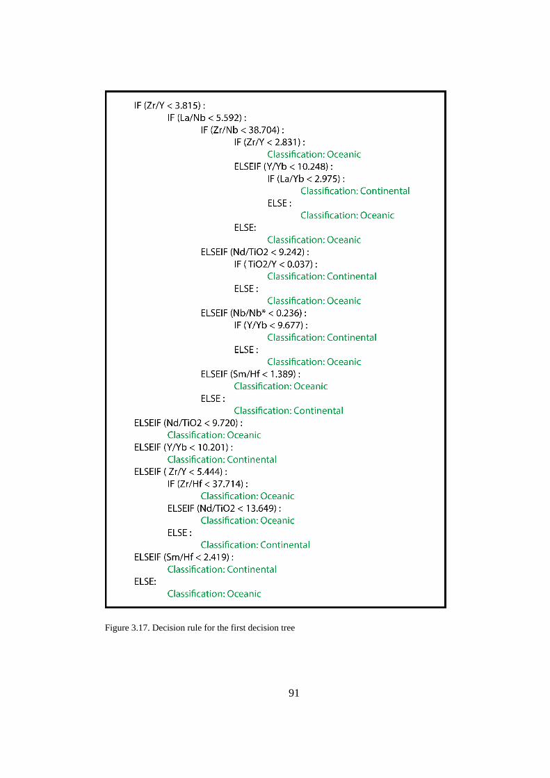
91
Figure 3.17. Decision rule for the first decision tree

92
Figure 3.18. Decision rule for the second decision tree
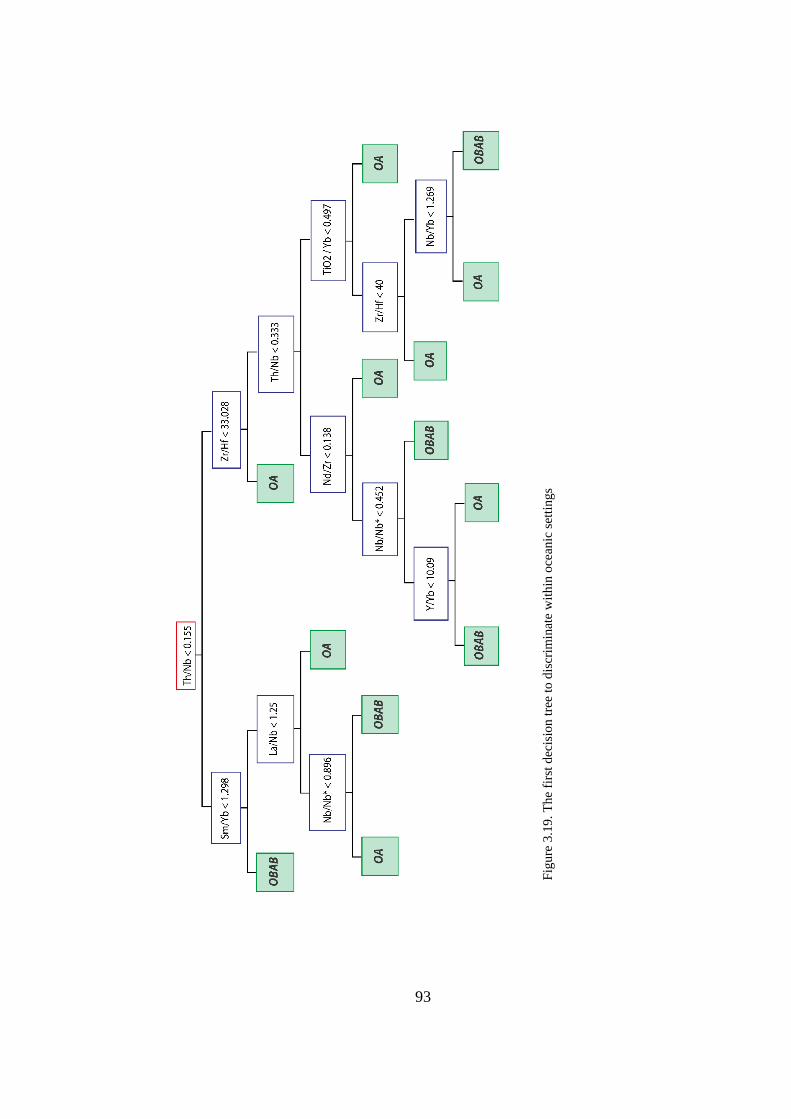
93
Figure 3.19. The first decision tree to discriminate within oceanic settings
Fig
ure
3.1
9.
The
firs
t d
ecis
ion
tre
e to
dis
crim
inat
e w
ith
in o
cean
ic s
etti
ng
s

94
Figure 3.20. The second decision tree to discriminate within oceanic settings
Fig
ure
3.2
0.
The
seco
nd
dec
isio
n t
ree
to d
iscr
imin
ate
wit
hin
oce
anic
set
tin
gs

95
Figure 3.21. Decision rule for the first decision tree
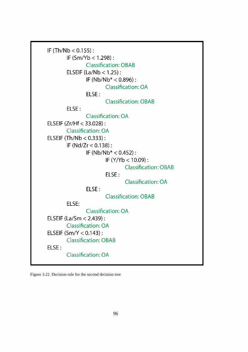
96
Figure 3.22. Decision rule for the second decision tree
97
3.1.3. Discrimination Within Non-Subduction Settings
The third set of decision trees is constructed for the tectono-magmatic discrimination
within non-subduction settings. Subduction settings are MOR, OP, OI and CWP. At
first stage, MOR and OP (Group 1) are discriminated from OI and CWP (Group 2). If
the sample is classified as Group 1, a further discrimination is required between MOR
and OP. If the sample is classified as Group 2, a discrimination is applied between OI
and CWP.
3.1.3.1. Discrimination Between Group 1 (Mid-Oceanic Ridge and Oceanic
Plateau) and Group 2 (Oceanic Island and Continental Within-plate) Settings
The first step of discrimination within non-subduction settings is discrimination of
samples into two sub-groups: group 1 consisting samples of mid-oceanic ridges and
oceanic plateaus and group 2 consisting samples of oceanic islands and continental
within-plates.
Two decision trees are constructed for the tectono-magmatic discrimination within
non-subduction settings (MOR and OP as Group 1, OI and CWP as Group 2). Both
decision trees have 7 levels of depth. The first decision tree uses Sm/Yb at first level,
Nd/Zr at second level, Th/Nb and Y/Yb at third level, Zr/TiO2, La/Nb, Nb/Nb* and
La/Sm at fourth level, La/Nb, Nd/Zr and Nb/Yb at fifth level, TiO2/Y, Nb/Nb* and
Th/Nb at sixth level and Zr/Hf and Th/La at seventh level (Figure 3.23).
The second decision tree uses Sm/Yb at first level, Nd/Zr at second level, Th/Nb and
Y/Yb at third level, Th/La, La/Nb, Nb/Nb* and La/Sm at fourth level, Sm/Hf, Nd/Zr
and Nb/Yb at fifth level, La/Nb, Nb/Nb* and Th/Nb at sixth level and Nb/Y, Zr/Hf
and Th/La at seventh level (Figure 3.24).
Decision rules for constructed decision trees are given in Figure 3.25 and Figure 3.26,
respectively.
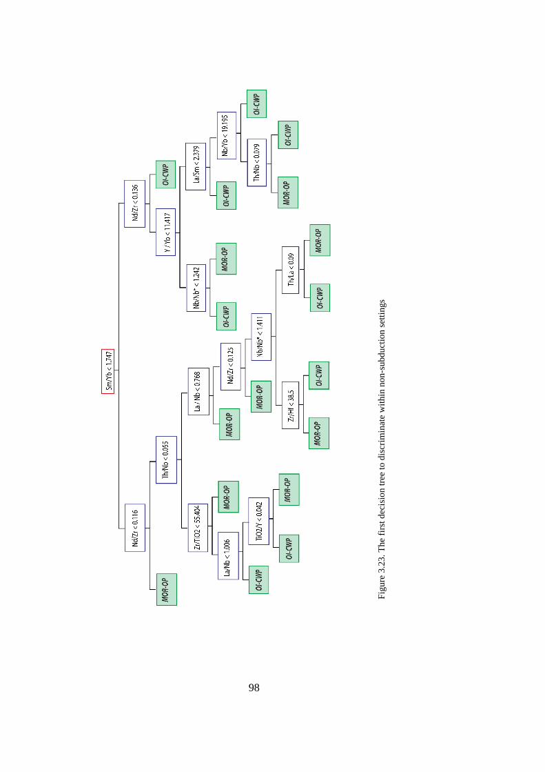
98
Figure 3.23. The first decision tree to discriminate within non-subduction settings
Fig
ure
3.2
3.
The
firs
t d
ecis
ion
tre
e to
dis
crim
inat
e w
ith
in n
on
-su
bd
uct
ion
set
tin
gs
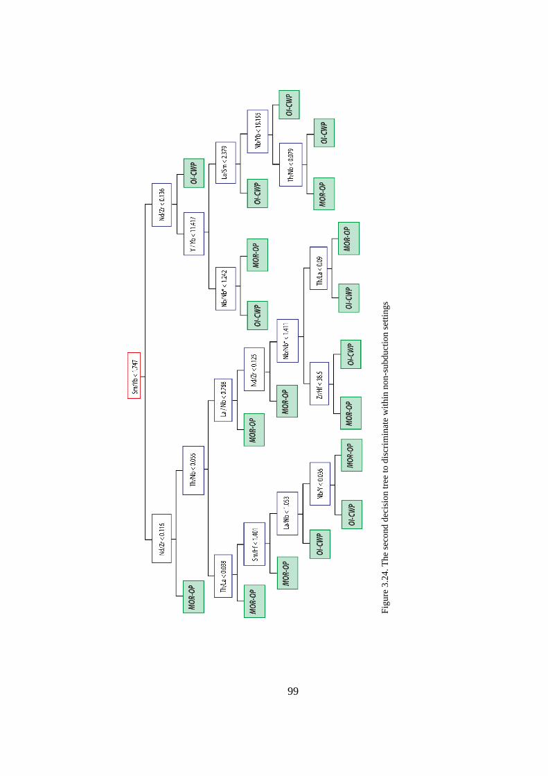
99
Figure 3.24. The second decision tree to discriminate within non-subduction settings
Fig
ure
3.2
4.
The
seco
nd
dec
isio
n t
ree
to d
iscr
imin
ate
wit
hin
no
n-s
ubd
uct
ion
set
tin
gs
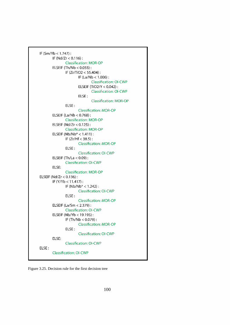
100
Figure 3.25. Decision rule for the first decision tree
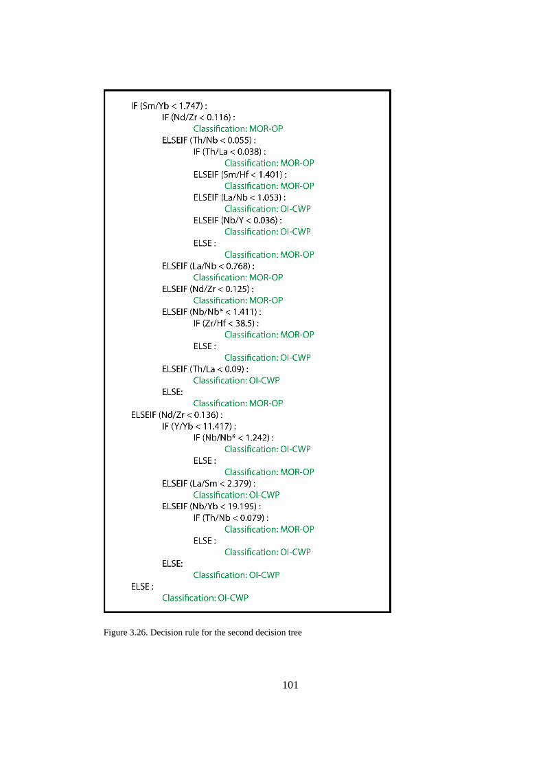
101
Figure 3.26. Decision rule for the second decision tree
102
3.1.3.2. Discrimination Between Mid-Oceanic Ridges and Oceanic Plateaus
Two decision trees are constructed for the tectono-magmatic discrimination between
MOR and OP. The first decision tree has 6 and the second one has 7 levels of depth.
The first decision tree uses Th/Y at first level, Zr/Hf at second level, Nb/ TiO2 at third
level, Th/Y and Zr/Y at fourth level, Zr/Y, Zr/Nb, and Th/La at fifth level, Th/La and
Nb/Nb* at sixth level (Figure 3.27).
The second decision tree uses Th/Y at first level, Zr/Hf at second level, Zr/Nb at third
level, Sm/Yb and Zr/Hf at fourth level, Zr/Nb, La/Nb, Y/Yb and Zr/Hf at fifth level,
Th/La, La/Y and Zr/Nb at sixth level and Sm/Y at seventh level (Figure 3.28).
Decision rules for constructed decision trees are given in Figure 3.29 and Figure 3.30,
respectively.
3.1.3.3. Discrimination Between Oceanic Islands and Continental Within-plates
Two decision trees are constructed for the tectono-magmatic discrimination between
OI and CWP. Both decision trees have 8 levels of depth. The first decision tree uses
Nb/Y at first level, Zr/Yb at second and third levels, Sm/Nb and Zr/Y at fourth level,
Th/Nb and TiO2/Y at fifth level, Th/Nb, Nb/ TiO2, Y/Yb and Zr/Hf at sixth level,
Sm/Nd, Th/La, Sm/Yb, Nb/Y and Th/La at seventh level and La/Y, Zr/Nb, Zr/Yb,
Sm/Nb and La/Sm at eighth level (Figure 3.31).
The second decision tree uses Nb/Y at first level, Zr/Yb at second and third levels,
Sm/Nb and Zr/Y at fourth level, Th/Nb and Sm/Nb at fifth level, Th/Nb, Sm/Nb, Zr/Y
and Zr/Hf at sixth level, Sm/Nd, Y/Yb, Zr/Yb and Nb/Yb at seventh level and La/Y,
Zr/Nb and Sm/Nd at eighth level (Figure 3.32).
Decision rules for constructed decision trees are given in Figure 3.33 and Figure 3.34,
respectively.
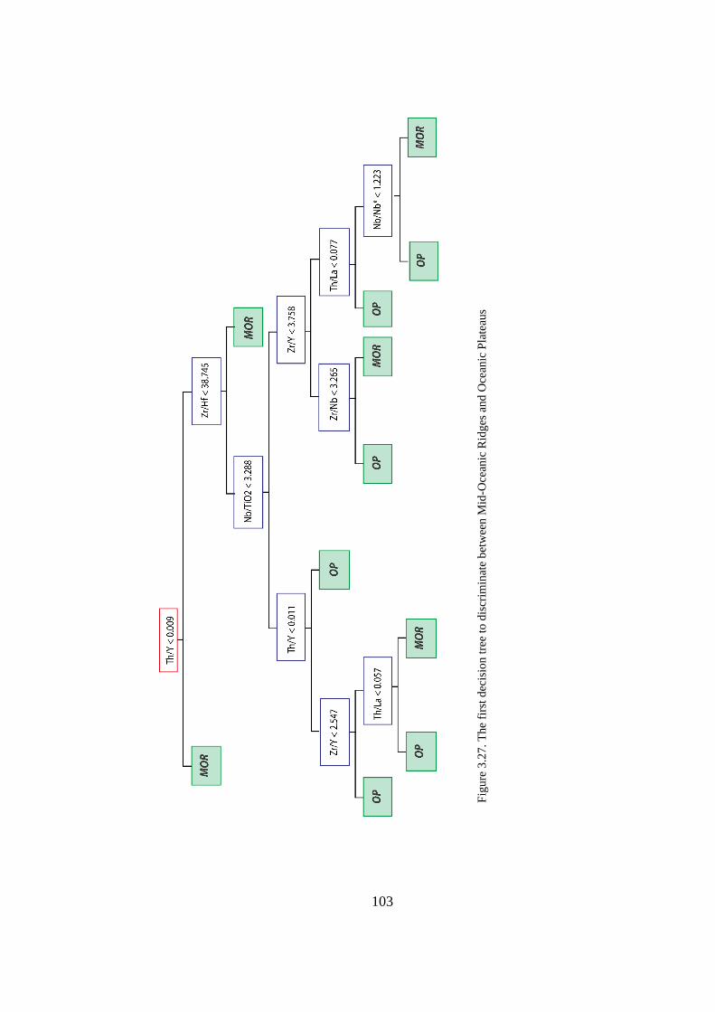
103
Figure 3.27. The first decision tree to discriminate between Mid-Oceanic Ridges and Oceanic Plateaus
Fig
ure
3.2
7.
The
firs
t d
ecis
ion
tre
e to
dis
crim
inat
e b
etw
een
Mid
-Oce
anic
Rid
ges
an
d O
cean
ic P
late
aus
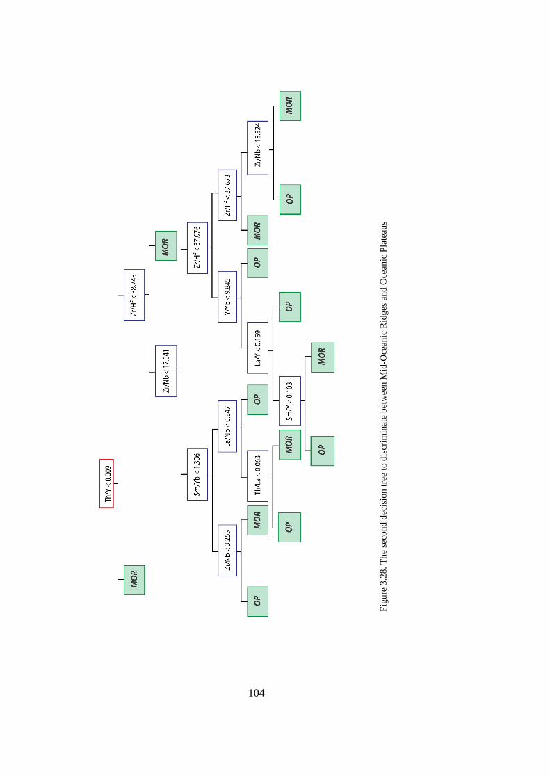
104
Figure 3.28. The second decision tree to discriminate between Mid-Oceanic Ridges and Oceanic Plateaus
Fig
ure
3.2
8.
The
seco
nd
dec
isio
n t
ree
to d
iscr
imin
ate
bet
wee
n M
id-O
cean
ic R
idg
es a
nd
Oce
anic
Pla
teau
s

105
Figure 3.29. Decision rule for the first decision tree
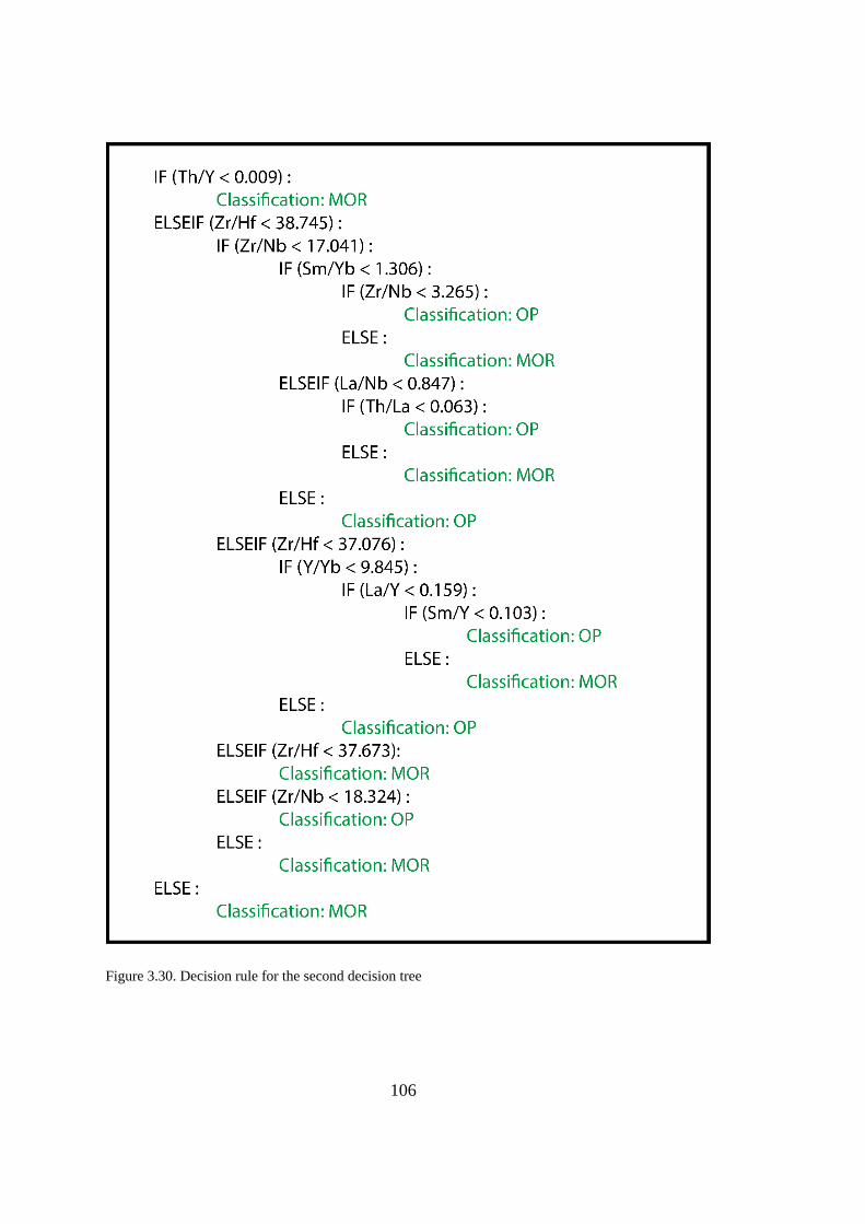
106
Figure 3.30. Decision rule for the second decision tree
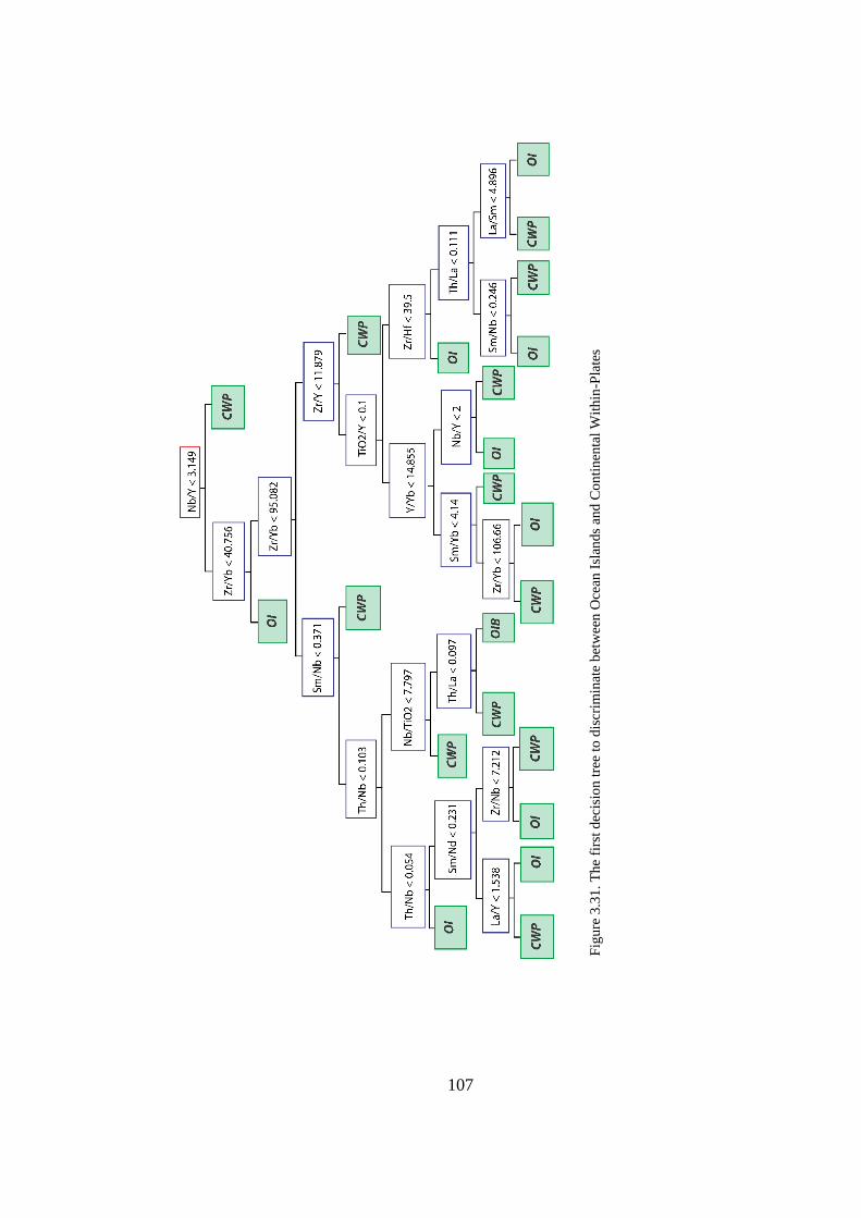
107
Figure 3.31. The first decision tree to discriminate between Ocean Islands and Continental Within-Plates
Fig
ure
3.3
1.
The
firs
t d
ecis
ion
tre
e to
dis
crim
inat
e b
etw
een
Oce
an I
slan
ds
and
Co
nti
nen
tal
Wit
hin
-Pla
tes
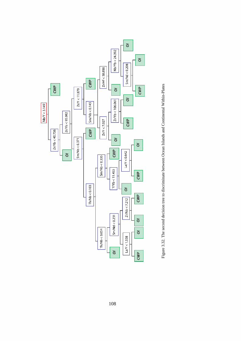
108
Figure 3.32. The second decision tree to discriminate between Ocean Islands and Continental Within-Plates
Fig
ure
3.3
2.
Th
e se
con
d d
ecis
ion
tre
e to
dis
crim
inat
e b
etw
een
Oce
an I
slan
ds
and
Con
tinen
tal
Wit
hin
-Pla
tes

109
Figure 3.33. Decision rule for the first decision tree
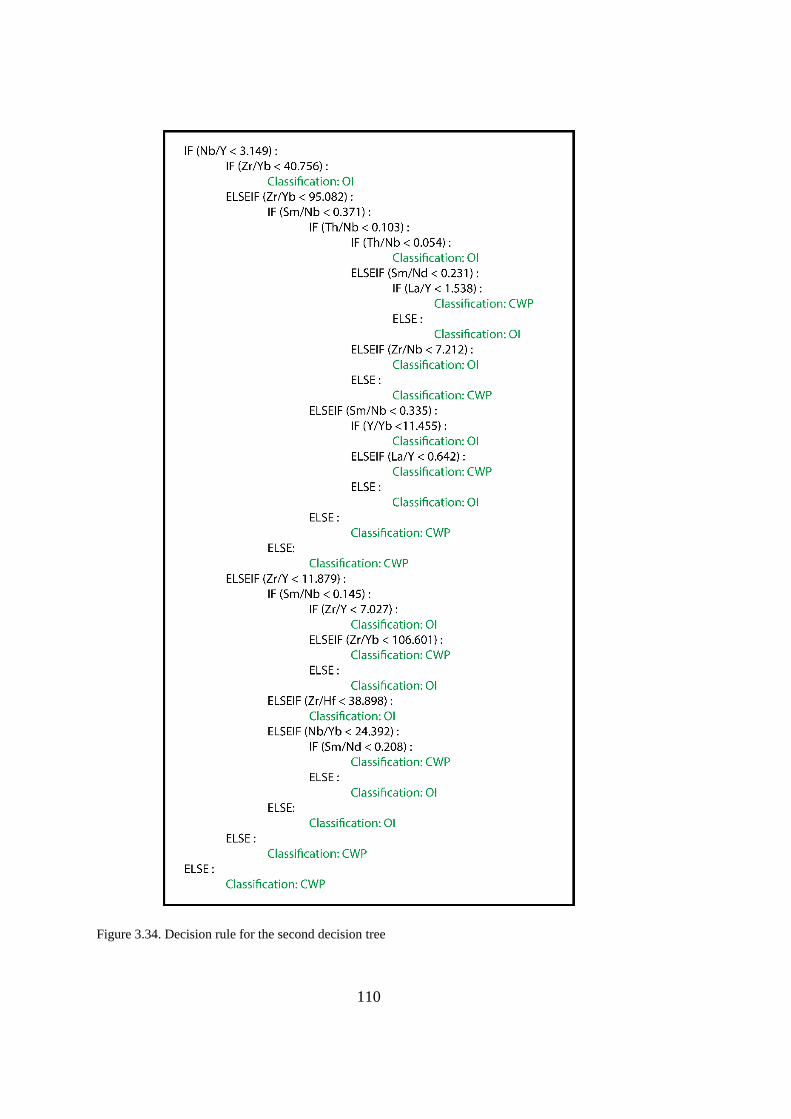
110
Figure 3.34. Decision rule for the second decision tree
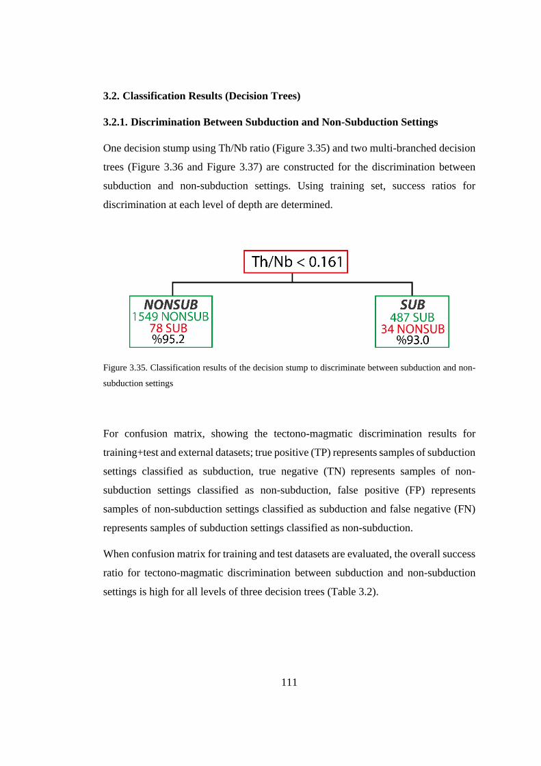
111
3.2. Classification Results (Decision Trees)
3.2.1. Discrimination Between Subduction and Non-Subduction Settings
One decision stump using Th/Nb ratio (Figure 3.35) and two multi-branched decision
trees (Figure 3.36 and Figure 3.37) are constructed for the discrimination between
subduction and non-subduction settings. Using training set, success ratios for
discrimination at each level of depth are determined.
Figure 3.35. Classification results of the decision stump to discriminate between subduction and non-
subduction settings
For confusion matrix, showing the tectono-magmatic discrimination results for
training+test and external datasets; true positive (TP) represents samples of subduction
settings classified as subduction, true negative (TN) represents samples of non-
subduction settings classified as non-subduction, false positive (FP) represents
samples of non-subduction settings classified as subduction and false negative (FN)
represents samples of subduction settings classified as non-subduction.
When confusion matrix for training and test datasets are evaluated, the overall success
ratio for tectono-magmatic discrimination between subduction and non-subduction
settings is high for all levels of three decision trees (Table 3.2).
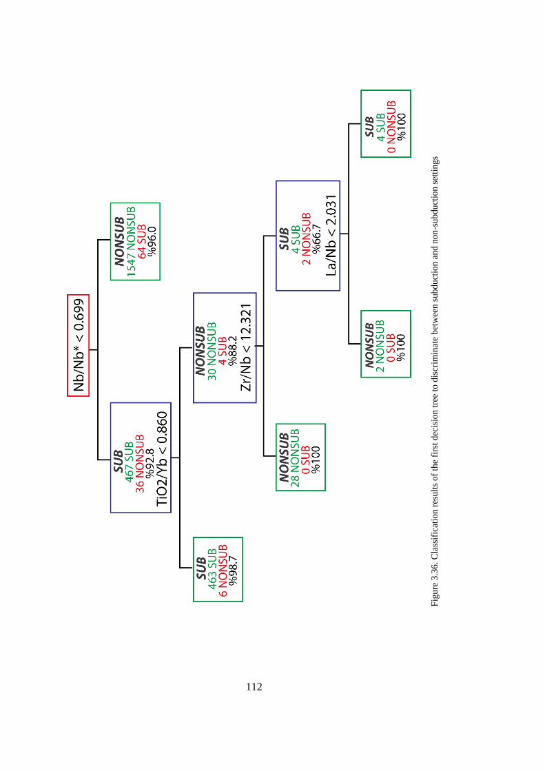
112
Figure 3.36. Classification results of the first decision tree to discriminate between subduction and non-subduction settings
Fig
ure
3.3
6.
Cla
ssif
icat
ion
res
ult
s of
the
firs
t dec
isio
n t
ree
to d
iscr
imin
ate
bet
wee
n s
ubd
uct
ion
an
d n
on
-su
bdu
ctio
n s
etti
ng
s
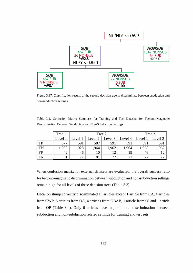
113
Figure 3.37. Classification results of the second decision tree to discriminate between subduction and
non-subduction settings
Table 3.2. Confusion Matrix Summary for Training and Test Datasets for Tectono-Magmatic
Discrimination Between Subduction and Non-Subduction Settings
Tree 1 Tree 2 Tree 3
Level 1 Level 1 Level 2 Level 3 Level 4 Level 1 Level 2
TP 577 591 587 591 591 591 591
TN 1,932 1,928 1,964 1,962 1,964 1,928 1,962
FP 42 46 10 12 19 46 12
FN 91 77 81 77 77 77 77
When confusion matrix for external datasets are evaluated, the overall success ratio
for tectono-magmatic discrimination between subduction and non-subduction settings
remain high for all levels of three decision trees (Table 3.3).
Decision stump correctly discriminated all articles except 1 article from CA, 4 articles
from CWP, 6 articles from OA, 4 articles from OBAB, 1 article from OI and 1 article
from OP (Table 3.4). Only 6 articles have major fails at discrimination between
subduction and non-subduction related settings for training and test sets.

114
Table 3.3. Confusion Matrix Summary for External Datasets for Tectono-Magmatic Discrimination
Between Subduction and Non-Subduction Settings
Tree 1 Tree 2 Tree 3
Level 1 Level 1 Level 2 Level 3 Level 4 Level 1 Level 2
TP 375 396 395 396 396 396 393
TN 1,937 1,942 1,981 1,977 1,977 1,942 1,979
FP 69 64 25 29 29 64 27
FN 91 70 71 70 70 70 73
Table 3.4. Misclassifications in training and test datasets by decision trump for discrimination between
subduction and non-subduction settings
JOU
RN
AL
CL
AS
S
SA
MP
LE
S
LE
VE
L 1
ER
RO
RS
LE
VE
L 1
ER
RO
R %
Mullen 2017 Cascade Arc CA 35 6 17.14
Coe 2008 South Africa CWP 27 23 85.19
Gibson 2000 Picrite CWP 16 3 18.75
Janney 2002 South Africa CWP 11 2 18.18
Mirnejad 2006 Leucite Hills CWP 10 10 100.00
Bedard 1999 Canada OA 12 2 16.67
Jolly 2007 Greater Antilles Arc OA 37 5 13.51
Jolly 2008 Greater Antilles Arc A OA 98 1 1.02
Pearce 2005 Mariana OA 11 1 9.09
Todd 2012 Fiji Tonga OA 13 5 38.46
Tollstrup 2010 Izu Bonin OA 51 2 3.92
Beier 2015 Manus Basin OBAB 6 5 83.33
Leat 2004 Sandwich OBAB 5 3 60.00
Pearce 1995 Lau OBAB 25 24 96.00
Pearce 2005 Mariana OBAB 53 33 62.26
Jackson 2010 Samoa OI 135 1 0.74
Neal 2002 Kerguelen OP 35 3 8.57
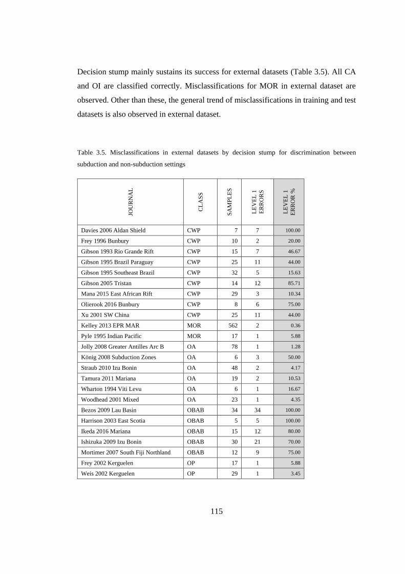
115
Decision stump mainly sustains its success for external datasets (Table 3.5). All CA
and OI are classified correctly. Misclassifications for MOR in external dataset are
observed. Other than these, the general trend of misclassifications in training and test
datasets is also observed in external dataset.
Table 3.5. Misclassifications in external datasets by decision stump for discrimination between
subduction and non-subduction settings
JOU
RN
AL
CL
AS
S
SA
MP
LE
S
LE
VE
L 1
ER
RO
RS
LE
VE
L 1
ER
RO
R %
Davies 2006 Aldan Shield CWP 7 7 100.00
Frey 1996 Bunbury CWP 10 2 20.00
Gibson 1993 Rio Grande Rift CWP 15 7 46.67
Gibson 1995 Brazil Paraguay CWP 25 11 44.00
Gibson 1995 Southeast Brazil CWP 32 5 15.63
Gibson 2005 Tristan CWP 14 12 85.71
Mana 2015 East African Rift CWP 29 3 10.34
Olierook 2016 Bunbury CWP 8 6 75.00
Xu 2001 SW China CWP 25 11 44.00
Kelley 2013 EPR MAR MOR 562 2 0.36
Pyle 1995 Indian Pacific MOR 17 1 5.88
Jolly 2008 Greater Antilles Arc B OA 78 1 1.28
König 2008 Subduction Zones OA 6 3 50.00
Straub 2010 Izu Bonin OA 48 2 4.17
Tamura 2011 Mariana OA 19 2 10.53
Wharton 1994 Viti Levu OA 6 1 16.67
Woodhead 2001 Mixed OA 23 1 4.35
Bezos 2009 Lau Basin OBAB 34 34 100.00
Harrison 2003 East Scotia OBAB 5 5 100.00
Ikeda 2016 Mariana OBAB 15 12 80.00
Ishizuka 2009 Izu Bonin OBAB 30 21 70.00
Mortimer 2007 South Fiji Northland OBAB 12 9 75.00
Frey 2002 Kerguelen OP 17 1 5.88
Weis 2002 Kerguelen OP 29 1 3.45
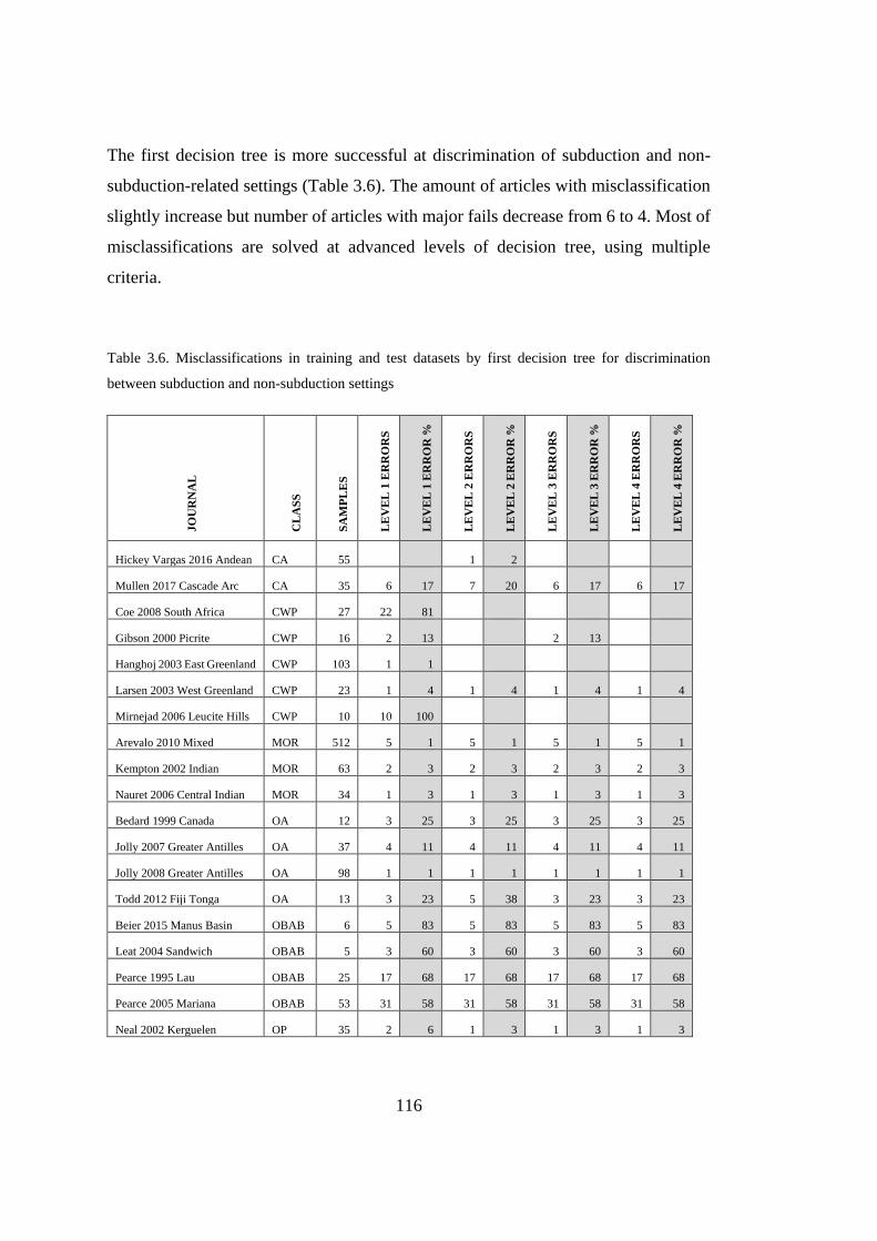
116
The first decision tree is more successful at discrimination of subduction and non-
subduction-related settings (Table 3.6). The amount of articles with misclassification
slightly increase but number of articles with major fails decrease from 6 to 4. Most of
misclassifications are solved at advanced levels of decision tree, using multiple
criteria.
Table 3.6. Misclassifications in training and test datasets by first decision tree for discrimination
between subduction and non-subduction settings
JO
UR
NA
L
CL
AS
S
SA
MP
LE
S
LE
VE
L 1
ER
RO
RS
LE
VE
L 1
ER
RO
R %
LE
VE
L 2
ER
RO
RS
LE
VE
L 2
ER
RO
R %
LE
VE
L 3
ER
RO
RS
LE
VE
L 3
ER
RO
R %
LE
VE
L 4
ER
RO
RS
LE
VE
L 4
ER
RO
R %
Hickey Vargas 2016 Andean CA 55 1 2
Mullen 2017 Cascade Arc CA 35 6 17 7 20 6 17 6 17
Coe 2008 South Africa CWP 27 22 81
Gibson 2000 Picrite CWP 16 2 13 2 13
Hanghoj 2003 East Greenland CWP 103 1 1
Larsen 2003 West Greenland CWP 23 1 4 1 4 1 4 1 4
Mirnejad 2006 Leucite Hills CWP 10 10 100
Arevalo 2010 Mixed MOR 512 5 1 5 1 5 1 5 1
Kempton 2002 Indian MOR 63 2 3 2 3 2 3 2 3
Nauret 2006 Central Indian MOR 34 1 3 1 3 1 3 1 3
Bedard 1999 Canada OA 12 3 25 3 25 3 25 3 25
Jolly 2007 Greater Antilles OA 37 4 11 4 11 4 11 4 11
Jolly 2008 Greater Antilles OA 98 1 1 1 1 1 1 1 1
Todd 2012 Fiji Tonga OA 13 3 23 5 38 3 23 3 23
Beier 2015 Manus Basin OBAB 6 5 83 5 83 5 83 5 83
Leat 2004 Sandwich OBAB 5 3 60 3 60 3 60 3 60
Pearce 1995 Lau OBAB 25 17 68 17 68 17 68 17 68
Pearce 2005 Mariana OBAB 53 31 58 31 58 31 58 31 58
Neal 2002 Kerguelen OP 35 2 6 1 3 1 3 1 3
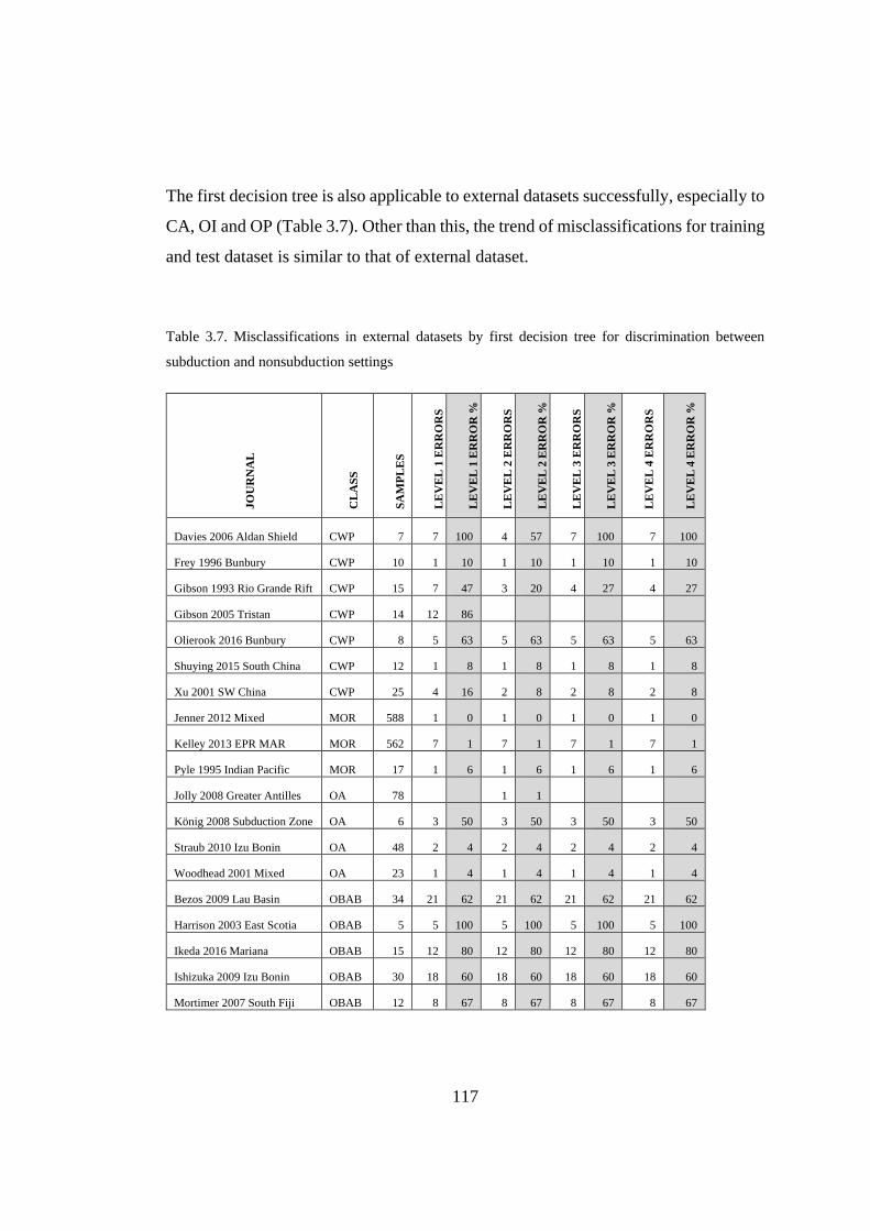
117
The first decision tree is also applicable to external datasets successfully, especially to
CA, OI and OP (Table 3.7). Other than this, the trend of misclassifications for training
and test dataset is similar to that of external dataset.
Table 3.7. Misclassifications in external datasets by first decision tree for discrimination between
subduction and nonsubduction settings
JO
UR
NA
L
CL
AS
S
SA
MP
LE
S
LE
VE
L 1
ER
RO
RS
LE
VE
L 1
ER
RO
R %
LE
VE
L 2
ER
RO
RS
LE
VE
L 2
ER
RO
R %
LE
VE
L 3
ER
RO
RS
LE
VE
L 3
ER
RO
R %
LE
VE
L 4
ER
RO
RS
LE
VE
L 4
ER
RO
R %
Davies 2006 Aldan Shield CWP 7 7 100 4 57 7 100 7 100
Frey 1996 Bunbury CWP 10 1 10 1 10 1 10 1 10
Gibson 1993 Rio Grande Rift CWP 15 7 47 3 20 4 27 4 27
Gibson 2005 Tristan CWP 14 12 86
Olierook 2016 Bunbury CWP 8 5 63 5 63 5 63 5 63
Shuying 2015 South China CWP 12 1 8 1 8 1 8 1 8
Xu 2001 SW China CWP 25 4 16 2 8 2 8 2 8
Jenner 2012 Mixed MOR 588 1 0 1 0 1 0 1 0
Kelley 2013 EPR MAR MOR 562 7 1 7 1 7 1 7 1
Pyle 1995 Indian Pacific MOR 17 1 6 1 6 1 6 1 6
Jolly 2008 Greater Antilles OA 78 1 1
König 2008 Subduction Zone OA 6 3 50 3 50 3 50 3 50
Straub 2010 Izu Bonin OA 48 2 4 2 4 2 4 2 4
Woodhead 2001 Mixed OA 23 1 4 1 4 1 4 1 4
Bezos 2009 Lau Basin OBAB 34 21 62 21 62 21 62 21 62
Harrison 2003 East Scotia OBAB 5 5 100 5 100 5 100 5 100
Ikeda 2016 Mariana OBAB 15 12 80 12 80 12 80 12 80
Ishizuka 2009 Izu Bonin OBAB 30 18 60 18 60 18 60 18 60
Mortimer 2007 South Fiji OBAB 12 8 67 8 67 8 67 8 67
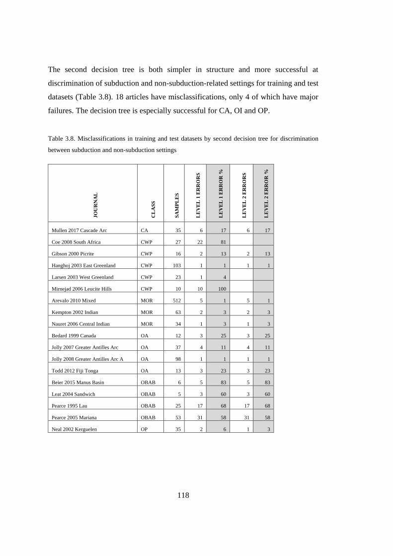
118
The second decision tree is both simpler in structure and more successful at
discrimination of subduction and non-subduction-related settings for training and test
datasets (Table 3.8). 18 articles have misclassifications, only 4 of which have major
failures. The decision tree is especially successful for CA, OI and OP.
Table 3.8. Misclassifications in training and test datasets by second decision tree for discrimination
between subduction and non-subduction settings
JO
UR
NA
L
CL
AS
S
SA
MP
LE
S
LE
VE
L 1
ER
RO
RS
LE
VE
L 1
ER
RO
R %
LE
VE
L 2
ER
RO
RS
LE
VE
L 2
ER
RO
R %
Mullen 2017 Cascade Arc CA 35 6 17 6 17
Coe 2008 South Africa CWP 27 22 81
Gibson 2000 Picrite CWP 16 2 13 2 13
Hanghoj 2003 East Greenland CWP 103 1 1 1 1
Larsen 2003 West Greenland CWP 23 1 4
Mirnejad 2006 Leucite Hills CWP 10 10 100
Arevalo 2010 Mixed MOR 512 5 1 5 1
Kempton 2002 Indian MOR 63 2 3 2 3
Nauret 2006 Central Indian MOR 34 1 3 1 3
Bedard 1999 Canada OA 12 3 25 3 25
Jolly 2007 Greater Antilles Arc OA 37 4 11 4 11
Jolly 2008 Greater Antilles Arc A OA 98 1 1 1 1
Todd 2012 Fiji Tonga OA 13 3 23 3 23
Beier 2015 Manus Basin OBAB 6 5 83 5 83
Leat 2004 Sandwich OBAB 5 3 60 3 60
Pearce 1995 Lau OBAB 25 17 68 17 68
Pearce 2005 Mariana OBAB 53 31 58 31 58
Neal 2002 Kerguelen OP 35 2 6 1 3
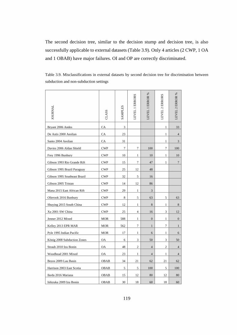
119
The second decision tree, similar to the decision stump and decision tree, is also
successfully applicable to external datasets (Table 3.9). Only 4 articles (2 CWP, 1 OA
and 1 OBAB) have major failures. OI and OP are correctly discriminated.
Table 3.9. Misclassifications in external datasets by second decision tree for discrimination between
subduction and non-subduction settings
JOU
RN
AL
CL
AS
S
SA
MP
LE
S
LE
VE
L 1
ER
RO
RS
LE
VE
L 1
ER
RO
R %
LE
VE
L 2
ER
RO
RS
LE
VE
L 2
ER
RO
R %
Bryant 2006 Andes CA 3 1 33
De Astis 2000 Aeolian CA 23 1 4
Santo 2004 Aeolian CA 31 1 3
Davies 2006 Aldan Shield CWP 7 7 100 7 100
Frey 1996 Bunbury CWP 10 1 10 1 10
Gibson 1993 Rio Grande Rift CWP 15 7 47 1 7
Gibson 1995 Brazil Paraguay CWP 25 12 48
Gibson 1995 Southeast Brazil CWP 32 5 16
Gibson 2005 Tristan CWP 14 12 86
Mana 2015 East African Rift CWP 29 1 3
Olierook 2016 Bunbury CWP 8 5 63 5 63
Shuying 2015 South China CWP 12 1 8 1 8
Xu 2001 SW China CWP 25 4 16 3 12
Jenner 2012 Mixed MOR 588 1 0 1 0
Kelley 2013 EPR MAR MOR 562 7 1 7 1
Pyle 1995 Indian Pacific MOR 17 1 6 1 6
König 2008 Subduction Zones OA 6 3 50 3 50
Straub 2010 Izu Bonin OA 48 2 4 2 4
Woodhead 2001 Mixed OA 23 1 4 1 4
Bezos 2009 Lau Basin OBAB 34 21 62 21 62
Harrison 2003 East Scotia OBAB 5 5 100 5 100
Ikeda 2016 Mariana OBAB 15 12 80 12 80
Ishizuka 2009 Izu Bonin OBAB 30 18 60 18 60
120
The trends of misclassifications for training – test datasets and external datasets are
similar to each other.
3.2.2. Discrimination Within Subduction Settings
3.2.2.1. The First Path for Discrimination Within Subduction Settings
The first path involves two-stage discrimination within subduction settings: (1)
between arc and back-arc-related settings, (2) within arc-related settings.
3.2.2.1.1. Discrimination Between Arc and Back-arc-related Settings
Two multi-branched decision trees (Figure 3.38 and Figure 3.39) are constructed for
the discrimination between arc and back-arc-related settings. Using training set,
success ratios for discrimination at each level of depth are determined.
For confusion matrix, showing the tectono-magmatic discrimination results for
training+test and external datasets; true positive (TP) represents samples of back-arc-
related settings classified as back-arc, true negative (TN) represents samples of arc-
related settings classified as arc, false positive (FP) represents samples of arc-related
settings classified as back-arc and false negative (FN) represents samples of back-arc-
related settings classified as arc.
When confusion matrix for training and test datasets are evaluated, the overall success
ratio for tectono-magmatic discrimination between arc and back-arc-related settings
are higher for the last two levels of two decision trees (Table 3.10).
When confusion matrix for external datasets are evaluated, the overall success ratio
for tectono-magmatic discrimination between arc and back-arc-related settings
decreases in varying degrees for the second trees (Table 3.11).
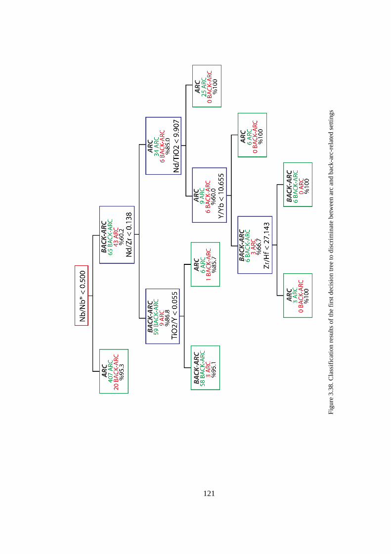
121
Figure 3.38. Classification results of the first decision tree to discriminate between arc and back-arc-related settings
Fig
ure
3.3
8.
Cla
ssif
icat
ion
res
ult
s of
the
firs
t d
ecis
ion
tre
e to
dis
crim
inat
e bet
wee
n a
rc a
nd b
ack
-arc
-rel
ated
set
tin
gs
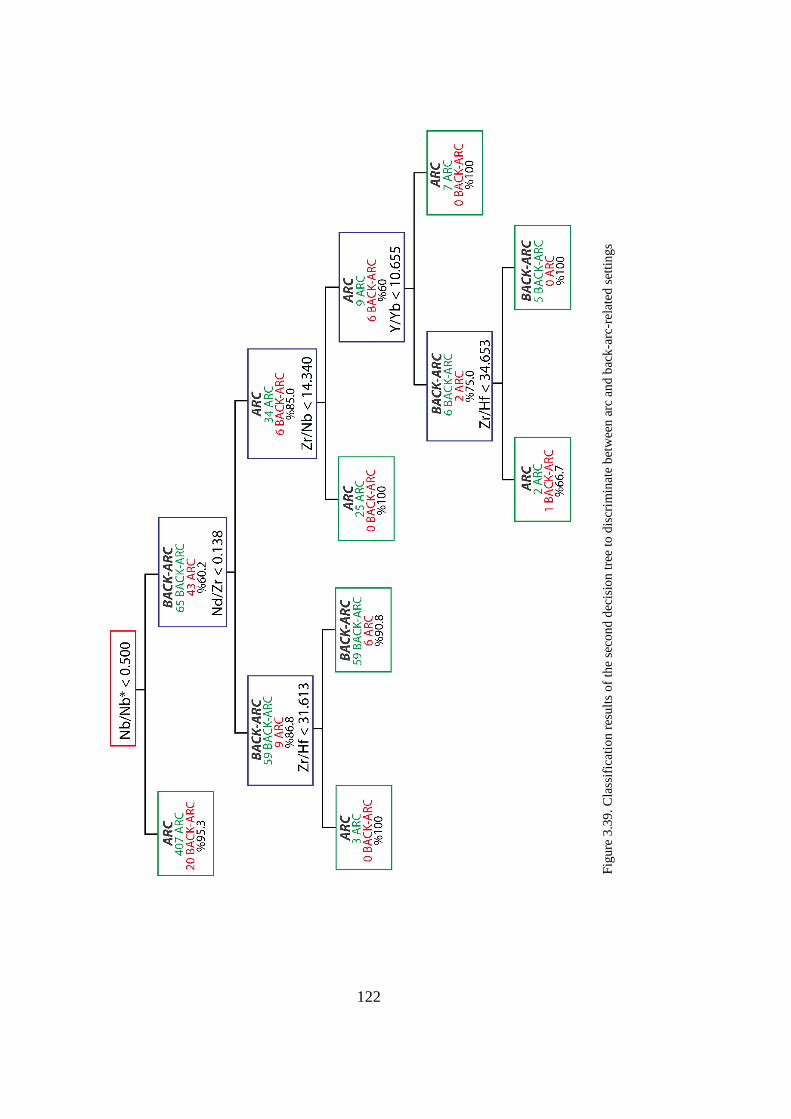
122
Figure 3.39. Classification results of the second decision tree to discriminate between arc and back-arc-related settings
Fig
ure
3.3
9.
Cla
ssif
icat
ion
res
ult
s of
the
seco
nd
dec
isio
n t
ree
to d
iscr
imin
ate
bet
wee
n a
rc a
nd
bac
k-a
rc-r
elat
ed s
etti
ng
s

123
Table 3.10. Confusion Matrix Summary for Training and Test Datasets for Tectono-Magmatic
Discrimination Between Arc and Back-arc-related Settings
Tree 1 2
Level 2 3 4 5 2 3 4 5
TP 86 84 92 92 86 82 89 88
TN 550 557 553 556 550 554 554 556
FP 12 5 9 6 12 8 8 6
FN 20 22
14 14 20 24 17 18
Table 3.11. Confusion Matrix Summary for External Datasets for Tectono-Magmatic Discrimination
Between Arc and Back-arc-related Settings
Tree 1 2
Level 2 3 4 5 2 3 4 5
TP 68 62 62 62 68 68 58 58
TN 348 348 347 347 348 354 350 351
FP 16 16 17 17 16 10 14 13
FN 34 40 40 40 34 34 44 44
The first decision tree correctly discriminated articles of subduction settings as arc-
related and back-arc-related settings except of 8 articles for training and test datasets
(Table 3.12). For this 8 articles, no major failures in discrimination is observed.
Misclassifications in the first levels are solved through the deeper levels in decision
tree.
The first decision tree is relatively more successful at OA and CA with respect to
OBAB for the discrimination of arc- and back-arc-related settings in training and test
datasets. Only 1 articles from OA has misclassification with a misclassification ratio
less than 10%.
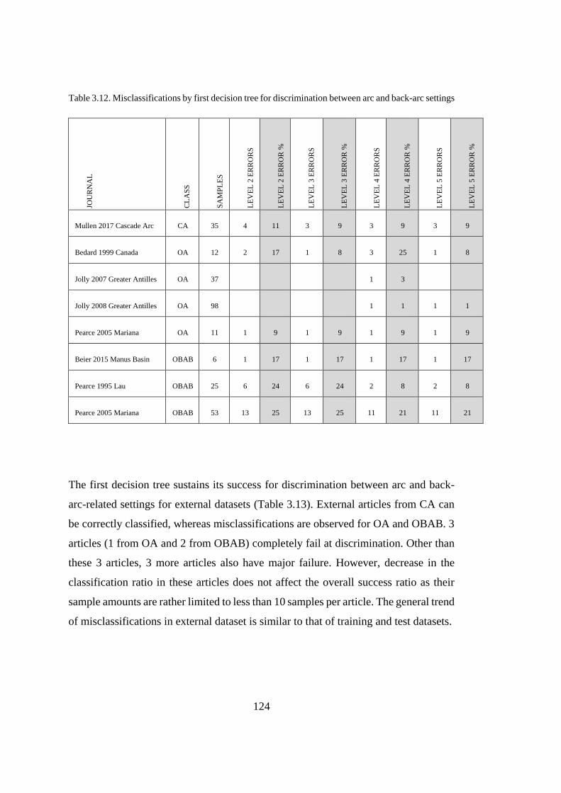
124
Table 3.12. Misclassifications by first decision tree for discrimination between arc and back-arc settings JO
UR
NA
L
CL
AS
S
SA
MP
LE
S
LE
VE
L 2
ER
RO
RS
LE
VE
L 2
ER
RO
R %
LE
VE
L 3
ER
RO
RS
LE
VE
L 3
ER
RO
R %
LE
VE
L 4
ER
RO
RS
LE
VE
L 4
ER
RO
R %
LE
VE
L 5
ER
RO
RS
LE
VE
L 5
ER
RO
R %
Mullen 2017 Cascade Arc CA 35 4 11 3 9 3 9 3 9
Bedard 1999 Canada OA 12 2 17 1 8 3 25 1 8
Jolly 2007 Greater Antilles OA 37 1 3
Jolly 2008 Greater Antilles OA 98 1 1 1 1
Pearce 2005 Mariana OA 11 1 9 1 9 1 9 1 9
Beier 2015 Manus Basin OBAB 6 1 17 1 17 1 17 1 17
Pearce 1995 Lau OBAB 25 6 24 6 24 2 8 2 8
Pearce 2005 Mariana OBAB 53 13 25 13 25 11 21 11 21
The first decision tree sustains its success for discrimination between arc and back-
arc-related settings for external datasets (Table 3.13). External articles from CA can
be correctly classified, whereas misclassifications are observed for OA and OBAB. 3
articles (1 from OA and 2 from OBAB) completely fail at discrimination. Other than
these 3 articles, 3 more articles also have major failure. However, decrease in the
classification ratio in these articles does not affect the overall success ratio as their
sample amounts are rather limited to less than 10 samples per article. The general trend
of misclassifications in external dataset is similar to that of training and test datasets.
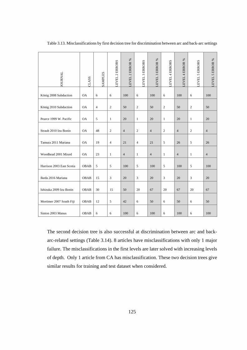
125
Table 3.13. Misclassifications by first decision tree for discrimination between arc and back-arc settings
JOU
RN
AL
CL
AS
S
SA
MP
LE
S
LE
VE
L 2
ER
RO
RS
LE
VE
L 2
ER
RO
R %
LE
VE
L 3
ER
RO
RS
LE
VE
L 3
ER
RO
R %
LE
VE
L 4
ER
RO
RS
LE
VE
L 4
ER
RO
R %
LE
VE
L 5
ER
RO
RS
LE
VE
L 5
ER
RO
R %
König 2008 Subduction OA 6 6 100 6 100 6 100 6 100
König 2010 Subduction OA 4 2 50 2 50 2 50 2 50
Pearce 1999 W. Pacific OA 5 1 20 1 20 1 20 1 20
Straub 2010 Izu Bonin OA 48 2 4 2 4 2 4 2 4
Tamura 2011 Mariana OA 19 4 21 4 21 5 26 5 26
Woodhead 2001 Mixed OA 23 1 4 1 4 1 4 1 4
Harrison 2003 East Scotia OBAB 5 5 100 5 100 5 100 5 100
Ikeda 2016 Mariana OBAB 15 3 20 3 20 3 20 3 20
Ishizuka 2009 Izu Bonin OBAB 30 15 50 20 67 20 67 20 67
Mortimer 2007 South Fiji OBAB 12 5 42 6 50 6 50 6 50
Sinton 2003 Manus OBAB 6 6 100 6 100 6 100 6 100
The second decision tree is also successful at discrimination between arc and back-
arc-related settings (Table 3.14). 8 articles have misclassifications with only 1 major
failure. The misclassifications in the first levels are later solved with increasing levels
of depth. Only 1 article from CA has misclassification. These two decision trees give
similar results for training and test dataset when considered.
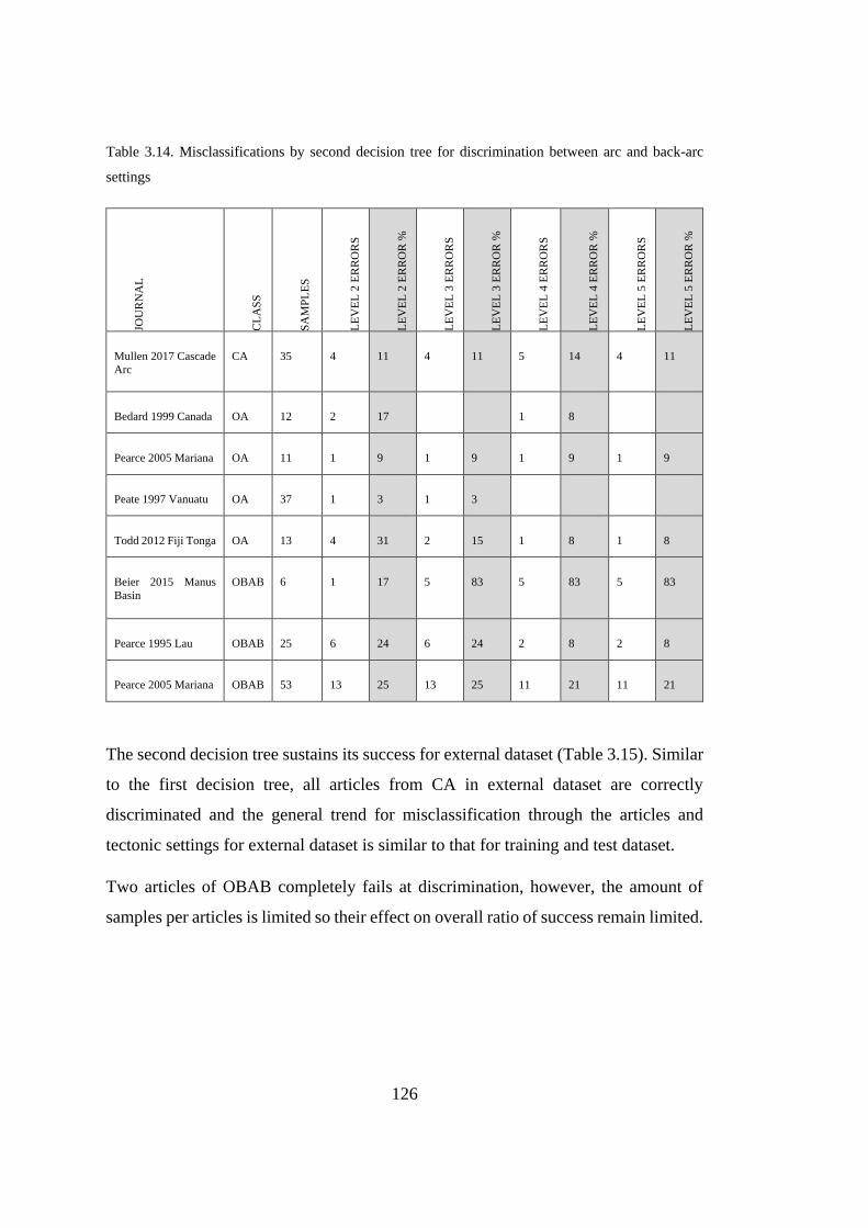
126
Table 3.14. Misclassifications by second decision tree for discrimination between arc and back-arc
settings
JOU
RN
AL
CL
AS
S
SA
MP
LE
S
LE
VE
L 2
ER
RO
RS
LE
VE
L 2
ER
RO
R %
LE
VE
L 3
ER
RO
RS
LE
VE
L 3
ER
RO
R %
LE
VE
L 4
ER
RO
RS
LE
VE
L 4
ER
RO
R %
LE
VE
L 5
ER
RO
RS
LE
VE
L 5
ER
RO
R %
Mullen 2017 Cascade
Arc
CA 35 4 11 4 11 5 14 4 11
Bedard 1999 Canada OA 12 2 17 1 8
Pearce 2005 Mariana OA 11 1 9 1 9 1 9 1 9
Peate 1997 Vanuatu OA 37 1 3 1 3
Todd 2012 Fiji Tonga OA 13 4 31 2 15 1 8 1 8
Beier 2015 Manus
Basin
OBAB 6 1 17 5 83 5 83 5 83
Pearce 1995 Lau OBAB 25 6 24 6 24 2 8 2 8
Pearce 2005 Mariana OBAB 53 13 25 13 25 11 21 11 21
The second decision tree sustains its success for external dataset (Table 3.15). Similar
to the first decision tree, all articles from CA in external dataset are correctly
discriminated and the general trend for misclassification through the articles and
tectonic settings for external dataset is similar to that for training and test dataset.
Two articles of OBAB completely fails at discrimination, however, the amount of
samples per articles is limited so their effect on overall ratio of success remain limited.

127
Table 3.15. Misclassifications by second decision tree for discrimination between arc and back-arc
settings
JOU
RN
AL
CL
AS
S
SA
MP
LE
S
LE
VE
L 2
ER
RO
RS
LE
VE
L 2
ER
RO
R %
LE
VE
L 3
ER
RO
RS
LE
VE
L 3
ER
RO
R %
LE
VE
L 4
ER
RO
RS
LE
VE
L 4
ER
RO
R %
LE
VE
L 5
ER
RO
RS
LE
VE
L 5
ER
RO
R %
Jolly 2008 Greater Antilles B OA 78 1 1
König 2008 Subduction OA 6 6 100 1 17 1 17 1 17
König 2010 Subduction OA 4 2 50 1 25 1 25 1 25
Pearce 1999 Western Pacific OA 5 1 20 1 20 1 20 1 20
Straub 2010 Izu Bonin OA 48 2 4 2 4 2 4 2 4
Tamura 2011 Mariana OA 19 4 21 4 21 6 32 6 32
Wharton 1994 Viti Levu OA 6 1 17 1 17
Woodhead 2001 Mixed OA 23 1 4 1 4 1 4 1 4
Harrison 2003 East Scotia OBAB 5 5 100 5 100 5 100 5 100
Ikeda 2016 Mariana OBAB 15 3 20 3 20 4 27 4 27
Ishizuka 2009 Izu Bonin OBAB 30 15 50 15 50 22 73 22 73
Mortimer 2007 South Fiji OBAB 12 5 42 5 42 7 58 7 58
Sinton 2003 Manus OBAB 6 6 100 6 100 6 100 6 100
3.2.2.1.2. Discrimination Within Arc-related Settings
Two multi-branched decision trees (Figure 3.40 and Figure 3.41) are constructed for
the discrimination within arc and related settings. Using training set, success ratios for
discrimination at each level of depth are determined.
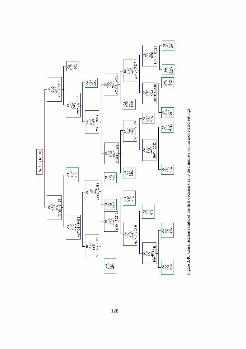
128
Figure 3.40. Classification results of the first decision tree to discriminate within arc-related settings
Fig
ure
3.4
0.
Cla
ssif
icat
ion
res
ult
s of
the
firs
t d
ecis
ion
tre
e to
dis
crim
inat
e w
ith
in a
rc-r
elat
ed s
etti
ng
s
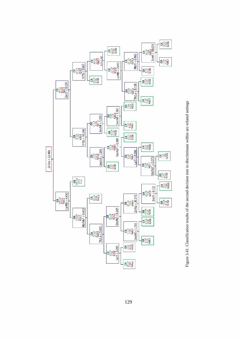
129
Figure 3.41. Classification results of the second decision tree to discriminate within arc-related settings
Fig
ure
3.4
1.
Cla
ssif
icat
ion
res
ult
s of
the
seco
nd
dec
isio
n t
ree
to d
iscr
imin
ate
wit
hin
arc
-rel
ated
set
tin
gs

130
For confusion matrix, showing the tectono-magmatic discrimination results for
training+test and external datasets; true positive (TP) represents samples of oceanic
arcs classified as oceanic arc, true negative (TN) represents samples of continental
arcs classified as continental arc, false positive (FP) represents samples of continental
arcs classified as oceanic arc and false negative (FN) represents samples oceanic arcs
classified as continental arc.
When confusion matrix for training and test datasets are evaluated, the overall success
ratio for tectono-magmatic discrimination between oceanic arc and continental arc
settings have an increasing trend with increasing levels in depth for both decision trees
(Table 3.16).
When their applicability to external datasets are evaluated, both decision trees with
their all levels shall be accepted to be applicable for tectono-magmatic discrimination
between oceanic arc and continental arc settings with a decrease in their success ratios
(Table 3.17).
Table 3.16. Confusion Matrix Summary for Training and Test Datasets for Tectono-Magmatic
Discrimination Between Oceanic Arc and Continental Arc Settings
Tree 1 2
Level 2 3 4 5 6 7 2 3 4 5 6 7
TP 308 298 368 367 362 370 360 360 352 367 372 368
TN 147 168 120 128 162 160 105 105 149 160 166 171
FP 34 13 61 53 19 21 76 76 32 21 15 10
FN 73 83 13 14 19 11 21 21 29 14 9 13
The first decision tree is successful at the discrimination between OA and CA (Table
3.18). The amount of articles with misclassifications are higher when compared to that
in previous discriminations. However, amount of misclassifications per articles are
small so that only 1 article has major failure at discrimination.

131
Table 3.17. Confusion Matrix Summary for External Dataset for Tectono-Magmatic Discrimination
Between Oceanic Arc and Continental Arc Settings
Tree 1 2
Level 2 3 4 5 6 7 2 3 4 5 6 7
TP 106 99 175 176 164 157 176 176 139 163 169 178
TN 136 136 83 68 75 72 54 54 73 95 108 107
FP 5 5 58 73 66 69 87 87 68 46 33 34
FN 117 124 48 47 59 66 47 47 84 60 54 45
The first decision tree is also applicable to external datasets yet, the amount of
misclassifications per articles slightly increase with more major failures. (Table 3.19).
The second decision tree is similar to the first decision tree for discrimination of
training and test dataset (Table 3.20) and for external dataset (Table 3.21). The trends
of misclassification are similar between first and second decision tree and between
training-test dataset and external dataset. There is no unexpected abrupt change in
success ratio for a specific tectonic setting or an article.
3.2.2.2. The Second Path for Discrimination Within Subduction Settings
3.2.2.2.1. Discrimination Between Oceanic and Continental Settings
Two multi-branched decision trees (Figure 3.42 and Figure 3.43) are constructed for
the discrimination between oceanic and continental settings. Using training set,
success ratios for discrimination at each level of depth are determined. For confusion
matrix, showing the tectono-magmatic discrimination results for training+test and
external datasets; true positive (TP) represents samples of oceanic settings classified
as oceanic, true negative (TN) represents samples of continental settings classified as
continental, false positive (FP) represents samples of continental settings classified as
oceanic and false negative (FN) represents samples of oceanic settings classified as
continental.

132
Table 3.18. Misclassifications by first decision tree for discrimination between oceanic arc and
continental-arc settings
JOU
RN
AL
CL
AS
S
SA
MP
LE
S
LE
VE
L 2
ER
RO
RS
LE
VE
L 2
ER
RO
R %
LE
VE
L 3
ER
RO
RS
LE
VE
L 3
ER
RO
R %
LE
VE
L 4
ER
RO
RS
LE
VE
L 4
ER
RO
R %
LE
VE
L 5
ER
RO
RS
LE
VE
L 5
ER
RO
R %
LE
VE
L 6
ER
RO
RS
LE
VE
L 6
ER
RO
R %
LE
VE
L 7
ER
RO
RS
LE
VE
L 7
ER
RO
R %
Gertisser 2000 Aeolian CA 5 1 20 1 20 4 80
Hickey Vargas 2016 Andean CA 55 1 2 1 2 8 15 8 15 3 5 5 9
Hickey Vargas 2016 Chile CA 34 1 3 1 3 26 76 26 76 1 3 4 12
Metrich 2001 Aeolian CA 10 2 20 2 20 2 20 2 20
Mullen 2017 Cascade Arc CA 35 9 26 9 26 18 51 11 31 11 31 3 9
Portnyagin 2015 Kamchatka CA 3 3 100 3 100
Simon 2014 Kamchatka CA 39 23 59 2 5 3 8 2 5 2 5 3 8
Bedard 1999 Canada OA 12 5 42 5 42 5 42
Hickey Vargas 2013 Daito OA 8 4 50 4 50 2 25 1 13
Jolly 2007 Greater Antilles OA 37 14 38 14 38 3 8 3 8 4 11 1 3
Jolly 2008 Greater Antilles OA 98 15 15 20 20 8 8 7 7 8 8 1 1
Pearce 1995 South Sandwich OA 14 1 7 1 7
Pearce 2005 Mariana OA 11 2 18 2 18
Peate 1997 Vanuatu OA 37 8 22 10 27 1 3 5 14 4 11 2 5
Rojas Agramonte 2017
Lesser Antilles
OA 15 9 60 9 60 3 20 3 20 4 27 4 27
Singer 2007 Auletian OA 48 18 38 18 38 8 17 4 8
Todd 2012 Fiji Tonga OA 13 2 15 2 15 2 15 1 8 3 23
Tollstrup 2010 Izu Bonin OA 51 4 8 7 14 1 2 1 2 3 6 2 4
Yogodzinski 2015 Western
Auletian
OA 19 7 37 7 37
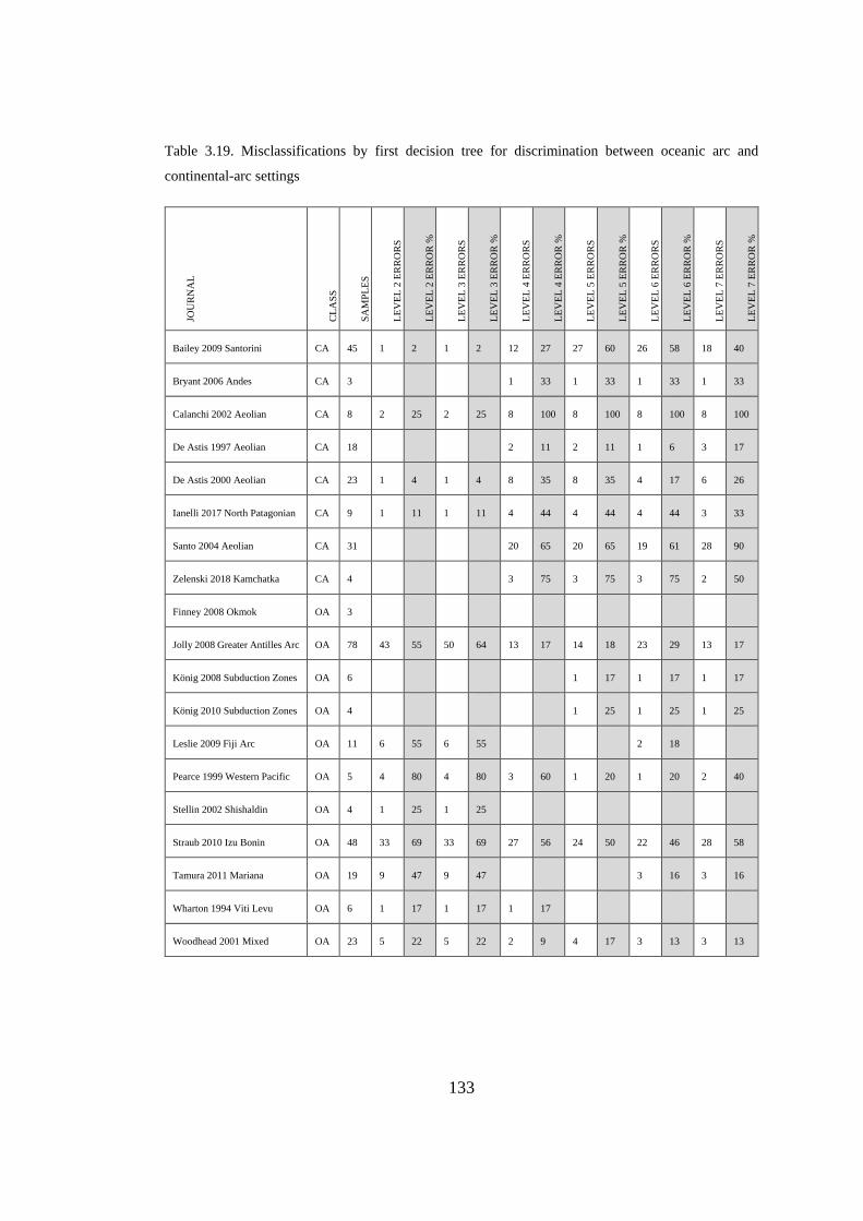
133
Table 3.19. Misclassifications by first decision tree for discrimination between oceanic arc and
continental-arc settings JO
UR
NA
L
CL
AS
S
SA
MP
LE
S
LE
VE
L 2
ER
RO
RS
LE
VE
L 2
ER
RO
R %
LE
VE
L 3
ER
RO
RS
LE
VE
L 3
ER
RO
R %
LE
VE
L 4
ER
RO
RS
LE
VE
L 4
ER
RO
R %
LE
VE
L 5
ER
RO
RS
LE
VE
L 5
ER
RO
R %
LE
VE
L 6
ER
RO
RS
LE
VE
L 6
ER
RO
R %
LE
VE
L 7
ER
RO
RS
LE
VE
L 7
ER
RO
R %
Bailey 2009 Santorini CA 45 1 2 1 2 12 27 27 60 26 58 18 40
Bryant 2006 Andes CA 3 1 33 1 33 1 33 1 33
Calanchi 2002 Aeolian CA 8 2 25 2 25 8 100 8 100 8 100 8 100
De Astis 1997 Aeolian CA 18 2 11 2 11 1 6 3 17
De Astis 2000 Aeolian CA 23 1 4 1 4 8 35 8 35 4 17 6 26
Ianelli 2017 North Patagonian CA 9 1 11 1 11 4 44 4 44 4 44 3 33
Santo 2004 Aeolian CA 31 20 65 20 65 19 61 28 90
Zelenski 2018 Kamchatka CA 4 3 75 3 75 3 75 2 50
Finney 2008 Okmok OA 3
Jolly 2008 Greater Antilles Arc OA 78 43 55 50 64 13 17 14 18 23 29 13 17
König 2008 Subduction Zones OA 6 1 17 1 17 1 17
König 2010 Subduction Zones OA 4 1 25 1 25 1 25
Leslie 2009 Fiji Arc OA 11 6 55 6 55 2 18
Pearce 1999 Western Pacific OA 5 4 80 4 80 3 60 1 20 1 20 2 40
Stellin 2002 Shishaldin OA 4 1 25 1 25
Straub 2010 Izu Bonin OA 48 33 69 33 69 27 56 24 50 22 46 28 58
Tamura 2011 Mariana OA 19 9 47 9 47 3 16 3 16
Wharton 1994 Viti Levu OA 6 1 17 1 17 1 17
Woodhead 2001 Mixed OA 23 5 22 5 22 2 9 4 17 3 13 3 13
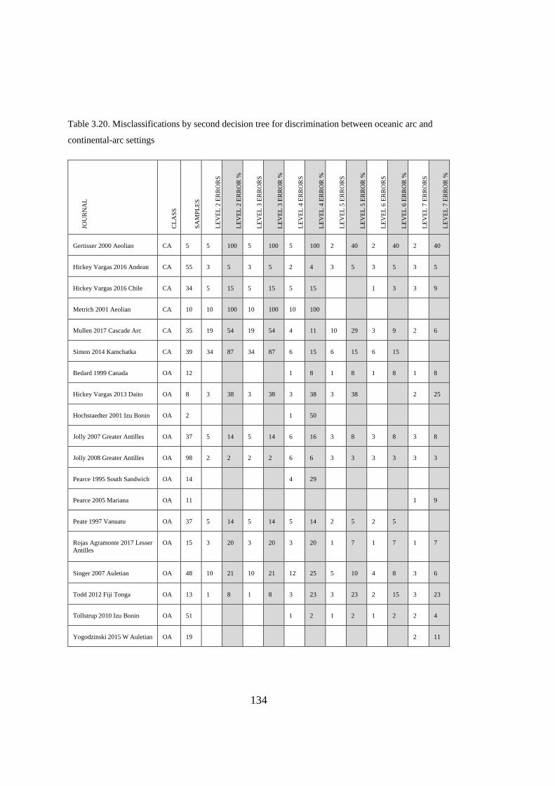
134
Table 3.20. Misclassifications by second decision tree for discrimination between oceanic arc and
continental-arc settings
JOU
RN
AL
CL
AS
S
SA
MP
LE
S
LE
VE
L 2
ER
RO
RS
LE
VE
L 2
ER
RO
R %
LE
VE
L 3
ER
RO
RS
LE
VE
L 3
ER
RO
R %
LE
VE
L 4
ER
RO
RS
LE
VE
L 4
ER
RO
R %
LE
VE
L 5
ER
RO
RS
LE
VE
L 5
ER
RO
R %
LE
VE
L 6
ER
RO
RS
LE
VE
L 6
ER
RO
R %
LE
VE
L 7
ER
RO
RS
LE
VE
L 7
ER
RO
R %
Gertisser 2000 Aeolian CA 5 5 100 5 100 5 100 2 40 2 40 2 40
Hickey Vargas 2016 Andean CA 55 3 5 3 5 2 4 3 5 3 5 3 5
Hickey Vargas 2016 Chile CA 34 5 15 5 15 5 15 1 3 3 9
Metrich 2001 Aeolian CA 10 10 100 10 100 10 100
Mullen 2017 Cascade Arc CA 35 19 54 19 54 4 11 10 29 3 9 2 6
Simon 2014 Kamchatka CA 39 34 87 34 87 6 15 6 15 6 15
Bedard 1999 Canada OA 12 1 8 1 8 1 8 1 8
Hickey Vargas 2013 Daito OA 8 3 38 3 38 3 38 3 38 2 25
Hochstaedter 2001 Izu Bonin OA 2 1 50
Jolly 2007 Greater Antilles OA 37 5 14 5 14 6 16 3 8 3 8 3 8
Jolly 2008 Greater Antilles OA 98 2 2 2 2 6 6 3 3 3 3 3 3
Pearce 1995 South Sandwich OA 14 4 29
Pearce 2005 Mariana OA 11 1 9
Peate 1997 Vanuatu OA 37 5 14 5 14 5 14 2 5 2 5
Rojas Agramonte 2017 Lesser
Antilles
OA 15 3 20 3 20 3 20 1 7 1 7 1 7
Singer 2007 Auletian OA 48 10 21 10 21 12 25 5 10 4 8 3 6
Todd 2012 Fiji Tonga OA 13 1 8 1 8 3 23 3 23 2 15 3 23
Tollstrup 2010 Izu Bonin OA 51 1 2 1 2 1 2 2 4
Yogodzinski 2015 W Auletian OA 19 2 11

135
Table 3.21. Misclassifications by second decision tree for discrimination between oceanic arc and
continental-arc settings JO
UR
NA
L
CL
AS
S
SA
MP
LE
S
LE
VE
L 2
ER
RO
RS
LE
VE
L 2
ER
RO
R %
LE
VE
L 3
ER
RO
RS
LE
VE
L 3
ER
RO
R %
LE
VE
L 4
ER
RO
RS
LE
VE
L 4
ER
RO
R %
LE
VE
L 5
ER
RO
RS
LE
VE
L 5
ER
RO
R %
LE
VE
L 6
ER
RO
RS
LE
VE
L 6
ER
RO
R %
LE
VE
L 7
ER
RO
RS
LE
VE
L 7
ER
RO
R %
Bailey 2009 Santorini CA 45 27 60 27 60 8 18 28 62 10 22 10 22
Bryant 2006 Andes CA 3 1 33 1 33 1 33
Calanchi 2002 Aeolian CA 8 8 100 8 100 8 100 1 13 2 25 2 25
De Astis 1997 Aeolian CA 18 10 56 10 56 10 56 3 17 3 17 3 17
De Astis 2000 Aeolian CA 23 14 61 14 61 14 61 4 17 5 22 5 22
Ianelli 2017 N Patagonian CA 9 2 22 2 22 2 22
Santo 2004 Aeolian CA 31 27 87 27 87 27 87 8 26 11 35 12 39
Jolly 2008 Antilles Arc B OA 78 18 23 18 23 22 28 27 35 18 23 10 13
König 2008 Subduction OA 6 2 33 2 33 2 33 2 33
König 2010 Subduction OA 4 3 75 3 75 3 75 3 75
Leslie 2009 Fiji Arc OA 11 1 9 1 9 1 9 1 9
Pearce 1999 W Pacific OA 5 1 20 1 20 1 20 1 20
Straub 2010 Izu Bonin OA 48 9 19 9 19 30 63 12 25 14 29 14 29
Tamura 2011 Mariana OA 19 4 21 4 21 4 21 4 21 4 21 3 16
Wharton 1994 Viti Levu OA 6 1 17 1 17 1 17 1 17
Woodhead 2001 Mixed OA 23 4 17 1 4 2 9 3 13
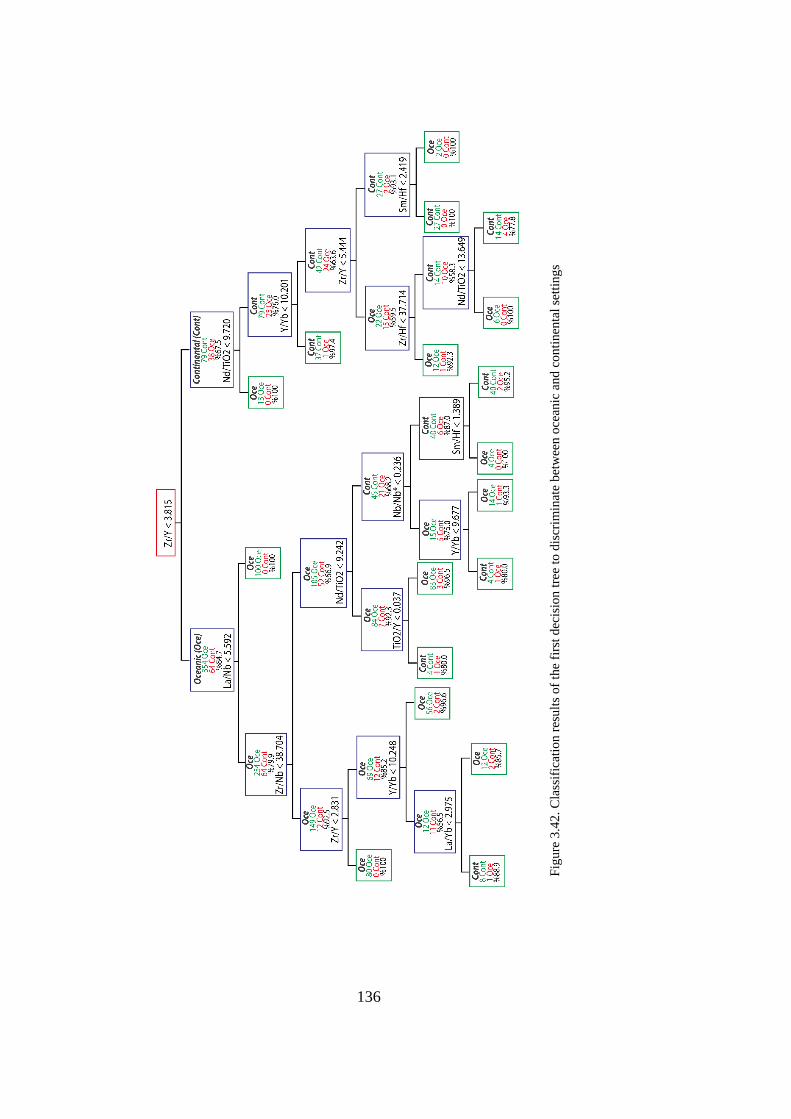
136
Figure 3.42. Classification results of the first decision tree to discriminate between oceanic and continental settings
Fig
ure
3.4
2.
Cla
ssif
icat
ion
res
ult
s of
the
firs
t d
ecis
ion
tre
e to
dis
crim
inat
e b
etw
een
oce
anic
an
d c
on
tin
enta
l se
ttin
gs

137
Figure 3.43. Classification results of the second decision tree to discriminate between oceanic and continental settings
Fig
ure
3.4
3.
Cla
ssif
icat
ion
res
ult
s of
the
seco
nd
dec
isio
n t
ree
to d
iscr
imin
ate
bet
wee
n o
cean
ic a
nd
co
nti
nen
tal
sett
ing
s
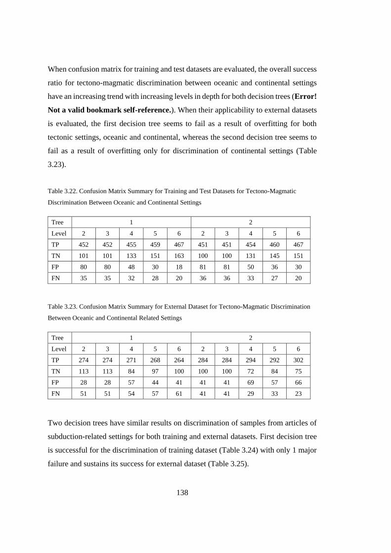
138
When confusion matrix for training and test datasets are evaluated, the overall success
ratio for tectono-magmatic discrimination between oceanic and continental settings
have an increasing trend with increasing levels in depth for both decision trees (Error!
Not a valid bookmark self-reference.). When their applicability to external datasets
is evaluated, the first decision tree seems to fail as a result of overfitting for both
tectonic settings, oceanic and continental, whereas the second decision tree seems to
fail as a result of overfitting only for discrimination of continental settings (Table
3.23).
Table 3.22. Confusion Matrix Summary for Training and Test Datasets for Tectono-Magmatic
Discrimination Between Oceanic and Continental Settings
Tree 1 2
Level 2 3 4 5 6 2 3 4 5 6
TP 452 452 455 459 467 451 451 454 460 467
TN 101 101 133 151 163 100 100 131 145 151
FP 80 80 48 30 18 81 81 50 36 30
FN 35 35 32 28 20 36 36 33 27 20
Table 3.23. Confusion Matrix Summary for External Dataset for Tectono-Magmatic Discrimination
Between Oceanic and Continental Related Settings
Tree 1 2
Level 2 3 4 5 6 2 3 4 5 6
TP 274 274 271 268 264 284 284 294 292 302
TN 113 113 84 97 100 100 100 72 84 75
FP 28 28 57 44 41 41 41 69 57 66
FN 51 51 54 57 61 41 41 29 33 23
Two decision trees have similar results on discrimination of samples from articles of
subduction-related settings for both training and external datasets. First decision tree
is successful for the discrimination of training dataset (Table 3.24) with only 1 major
failure and sustains its success for external dataset (Table 3.25).
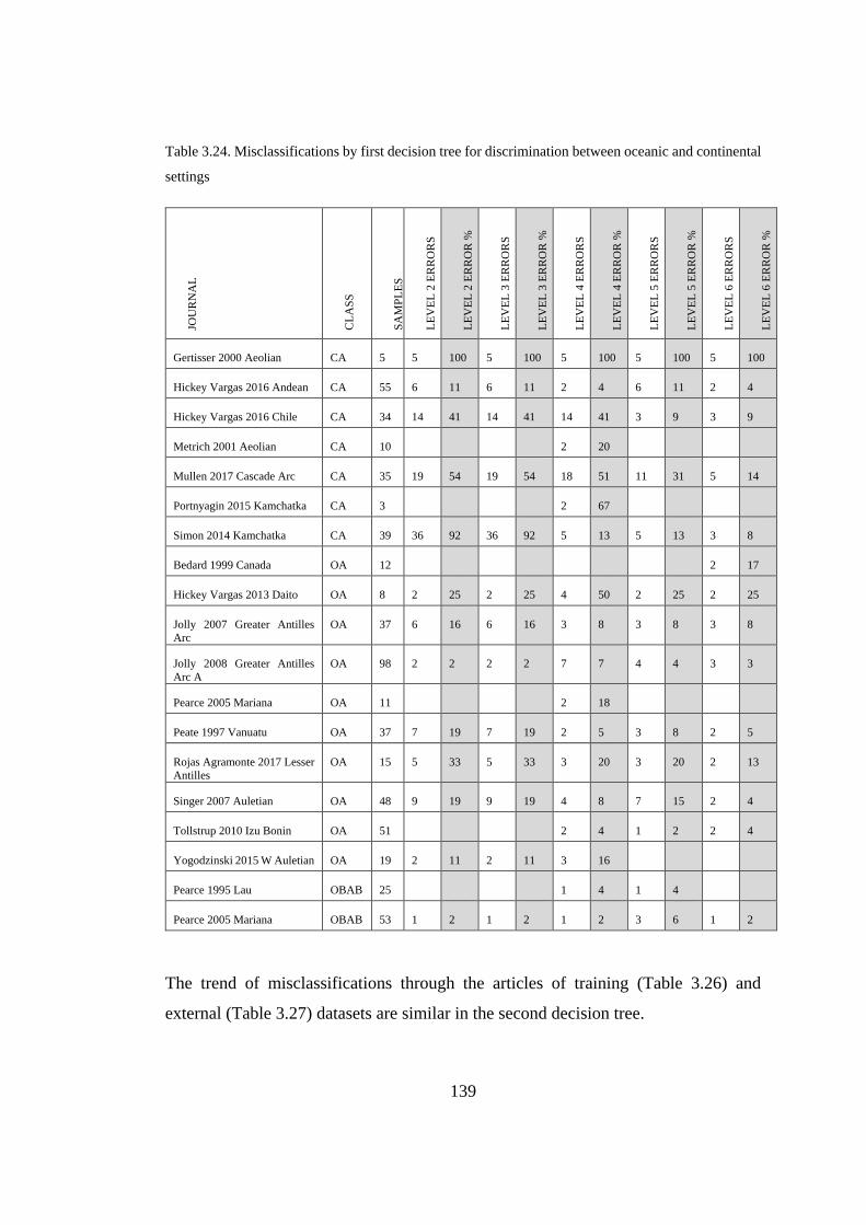
139
Table 3.24. Misclassifications by first decision tree for discrimination between oceanic and continental
settings JO
UR
NA
L
CL
AS
S
SA
MP
LE
S
LE
VE
L 2
ER
RO
RS
LE
VE
L 2
ER
RO
R %
LE
VE
L 3
ER
RO
RS
LE
VE
L 3
ER
RO
R %
LE
VE
L 4
ER
RO
RS
LE
VE
L 4
ER
RO
R %
LE
VE
L 5
ER
RO
RS
LE
VE
L 5
ER
RO
R %
LE
VE
L 6
ER
RO
RS
LE
VE
L 6
ER
RO
R %
Gertisser 2000 Aeolian CA 5 5 100 5 100 5 100 5 100 5 100
Hickey Vargas 2016 Andean CA 55 6 11 6 11 2 4 6 11 2 4
Hickey Vargas 2016 Chile CA 34 14 41 14 41 14 41 3 9 3 9
Metrich 2001 Aeolian CA 10 2 20
Mullen 2017 Cascade Arc CA 35 19 54 19 54 18 51 11 31 5 14
Portnyagin 2015 Kamchatka CA 3 2 67
Simon 2014 Kamchatka CA 39 36 92 36 92 5 13 5 13 3 8
Bedard 1999 Canada OA 12 2 17
Hickey Vargas 2013 Daito OA 8 2 25 2 25 4 50 2 25 2 25
Jolly 2007 Greater Antilles
Arc
OA 37 6 16 6 16 3 8 3 8 3 8
Jolly 2008 Greater Antilles
Arc A
OA 98 2 2 2 2 7 7 4 4 3 3
Pearce 2005 Mariana OA 11 2 18
Peate 1997 Vanuatu OA 37 7 19 7 19 2 5 3 8 2 5
Rojas Agramonte 2017 Lesser
Antilles
OA 15 5 33 5 33 3 20 3 20 2 13
Singer 2007 Auletian OA 48 9 19 9 19 4 8 7 15 2 4
Tollstrup 2010 Izu Bonin OA 51 2 4 1 2 2 4
Yogodzinski 2015 W Auletian OA 19 2 11 2 11 3 16
Pearce 1995 Lau OBAB 25 1 4 1 4
Pearce 2005 Mariana OBAB 53 1 2 1 2 1 2 3 6 1 2
The trend of misclassifications through the articles of training (Table 3.26) and
external (Table 3.27) datasets are similar in the second decision tree.
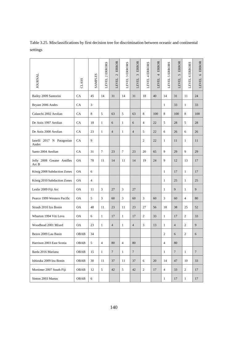
140
Table 3.25. Misclassifications by first decision tree for discrimination between oceanic and continental
settings
JOU
RN
AL
CL
AS
S
SA
MP
LE
S
LE
VE
L 2
ER
RO
RS
LE
VE
L
2
ER
RO
R
%
LE
VE
L 3
ER
RO
RS
LE
VE
L
3
ER
RO
R
%
LE
VE
L 4
ER
RO
RS
LE
VE
L
4
ER
RO
R
%
LE
VE
L 5
ER
RO
RS
LE
VE
L
5
ER
RO
R
%
LE
VE
L 6
ER
RO
RS
LE
VE
L
6
ER
RO
R
%
Bailey 2009 Santorini CA 45 14 31 14 31 18 40 14 31 11 24
Bryant 2006 Andes CA 3 1 33 1 33
Calanchi 2002 Aeolian CA 8 5 63 5 63 8 100 8 100 8 100
De Astis 1997 Aeolian CA 18 1 6 1 6 4 22 5 28 5 28
De Astis 2000 Aeolian CA 23 1 4 1 4 5 22 6 26 6 26
Ianelli 2017 N Patagonian
Andes
CA 9 2 22 1 11 1 11
Santo 2004 Aeolian CA 31 7 23 7 23 20 65 9 29 9 29
Jolly 2008 Greater Antilles
Arc B
OA 78 11 14 11 14 19 24 9 12 13 17
König 2008 Subduction Zones OA 6 1 17 1 17
König 2010 Subduction Zones OA 4 1 25 1 25
Leslie 2009 Fiji Arc OA 11 3 27 3 27 1 9 1 9
Pearce 1999 Western Pacific OA 5 3 60 3 60 3 60 3 60 4 80
Straub 2010 Izu Bonin OA 48 11 23 11 23 27 56 18 38 25 52
Wharton 1994 Viti Levu OA 6 1 17 1 17 2 33 1 17 2 33
Woodhead 2001 Mixed OA 23 1 4 1 4 3 13 1 4 2 9
Bezos 2009 Lau Basin OBAB 34 2 6 2 6
Harrison 2003 East Scotia OBAB 5 4 80 4 80 4 80
Ikeda 2016 Mariana OBAB 15 1 7 1 7 1 7 1 7
Ishizuka 2009 Izu Bonin OBAB 30 11 37 11 37 6 20 14 47 10 33
Mortimer 2007 South Fiji OBAB 12 5 42 5 42 2 17 4 33 2 17
Sinton 2003 Manus OBAB 6 1 17 1 17
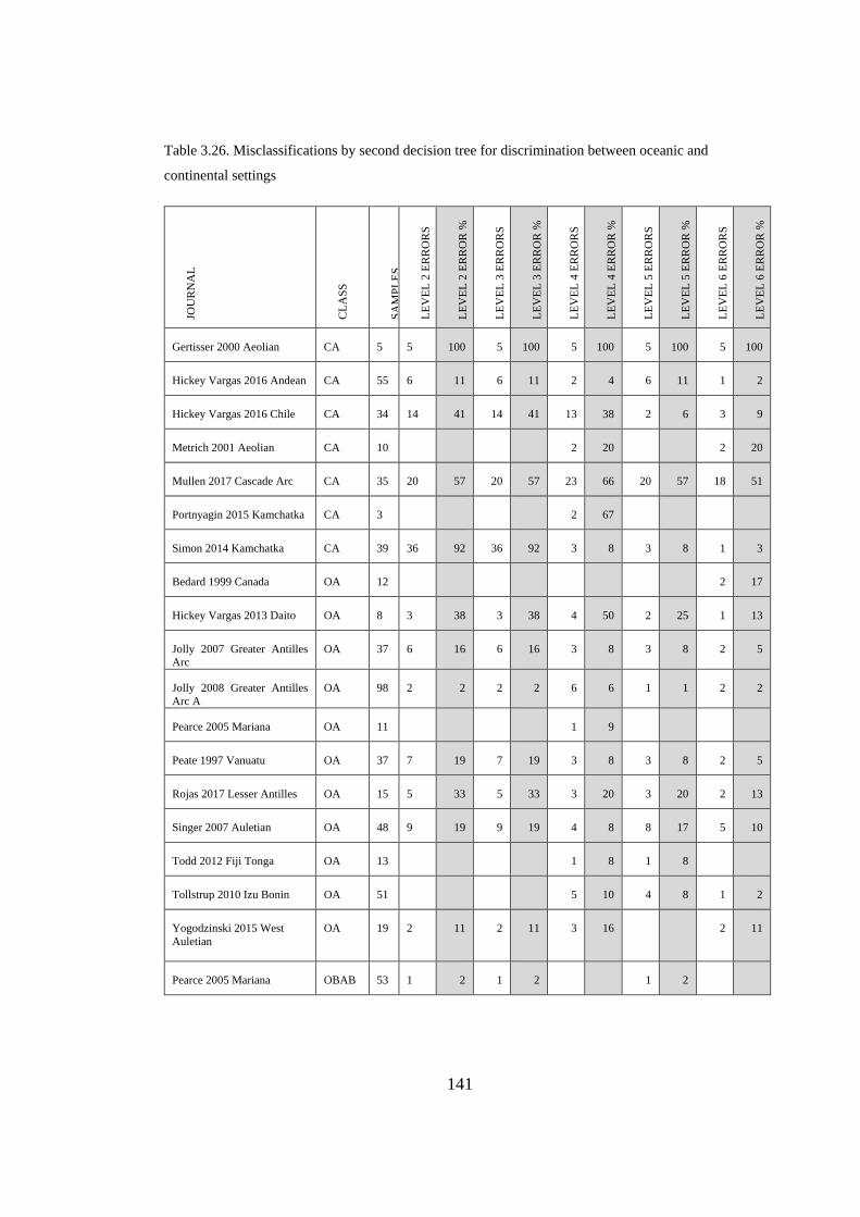
141
Table 3.26. Misclassifications by second decision tree for discrimination between oceanic and
continental settings JO
UR
NA
L
CL
AS
S
SA
MP
LE
S
LE
VE
L 2
ER
RO
RS
LE
VE
L 2
ER
RO
R %
LE
VE
L 3
ER
RO
RS
LE
VE
L 3
ER
RO
R %
LE
VE
L 4
ER
RO
RS
LE
VE
L 4
ER
RO
R %
LE
VE
L 5
ER
RO
RS
LE
VE
L 5
ER
RO
R %
LE
VE
L 6
ER
RO
RS
LE
VE
L 6
ER
RO
R %
Gertisser 2000 Aeolian CA 5 5 100 5 100 5 100 5 100 5 100
Hickey Vargas 2016 Andean CA 55 6 11 6 11 2 4 6 11 1 2
Hickey Vargas 2016 Chile CA 34 14 41 14 41 13 38 2 6 3 9
Metrich 2001 Aeolian CA 10 2 20 2 20
Mullen 2017 Cascade Arc CA 35 20 57 20 57 23 66 20 57 18 51
Portnyagin 2015 Kamchatka CA 3 2 67
Simon 2014 Kamchatka CA 39 36 92 36 92 3 8 3 8 1 3
Bedard 1999 Canada OA 12 2 17
Hickey Vargas 2013 Daito OA 8 3 38 3 38 4 50 2 25 1 13
Jolly 2007 Greater Antilles
Arc
OA 37 6 16 6 16 3 8 3 8 2 5
Jolly 2008 Greater Antilles
Arc A
OA 98 2 2 2 2 6 6 1 1 2 2
Pearce 2005 Mariana OA 11 1 9
Peate 1997 Vanuatu OA 37 7 19 7 19 3 8 3 8 2 5
Rojas 2017 Lesser Antilles OA 15 5 33 5 33 3 20 3 20 2 13
Singer 2007 Auletian OA 48 9 19 9 19 4 8 8 17 5 10
Todd 2012 Fiji Tonga OA 13 1 8 1 8
Tollstrup 2010 Izu Bonin OA 51 5 10 4 8 1 2
Yogodzinski 2015 West
Auletian
OA 19 2 11 2 11 3 16 2 11
Pearce 2005 Mariana OBAB 53 1 2 1 2 1 2
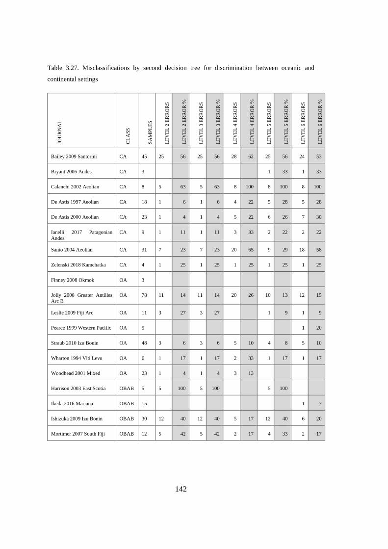
142
Table 3.27. Misclassifications by second decision tree for discrimination between oceanic and
continental settings
JOU
RN
AL
CL
AS
S
SA
MP
LE
S
LE
VE
L 2
ER
RO
RS
LE
VE
L 2
ER
RO
R %
LE
VE
L 3
ER
RO
RS
LE
VE
L 3
ER
RO
R %
LE
VE
L 4
ER
RO
RS
LE
VE
L 4
ER
RO
R %
LE
VE
L 5
ER
RO
RS
LE
VE
L 5
ER
RO
R %
LE
VE
L 6
ER
RO
RS
LE
VE
L 6
ER
RO
R %
Bailey 2009 Santorini CA 45 25 56 25 56 28 62 25 56 24 53
Bryant 2006 Andes CA 3 1 33 1 33
Calanchi 2002 Aeolian CA 8 5 63 5 63 8 100 8 100 8 100
De Astis 1997 Aeolian CA 18 1 6 1 6 4 22 5 28 5 28
De Astis 2000 Aeolian CA 23 1 4 1 4 5 22 6 26 7 30
Ianelli 2017 Patagonian
Andes
CA 9 1 11 1 11 3 33 2 22 2 22
Santo 2004 Aeolian CA 31 7 23 7 23 20 65 9 29 18 58
Zelenski 2018 Kamchatka CA 4 1 25 1 25 1 25 1 25 1 25
Finney 2008 Okmok OA 3
Jolly 2008 Greater Antilles
Arc B
OA 78 11 14 11 14 20 26 10 13 12 15
Leslie 2009 Fiji Arc OA 11 3 27 3 27 1 9 1 9
Pearce 1999 Western Pacific OA 5 1 20
Straub 2010 Izu Bonin OA 48 3 6 3 6 5 10 4 8 5 10
Wharton 1994 Viti Levu OA 6 1 17 1 17 2 33 1 17 1 17
Woodhead 2001 Mixed OA 23 1 4 1 4 3 13
Harrison 2003 East Scotia OBAB 5 5 100 5 100 5 100
Ikeda 2016 Mariana OBAB 15 1 7
Ishizuka 2009 Izu Bonin OBAB 30 12 40 12 40 5 17 12 40 6 20
Mortimer 2007 South Fiji OBAB 12 5 42 5 42 2 17 4 33 2 17
143
3.2.2.2.2. Discrimination Within Oceanic Settings
Two multi-branched decision trees (Figure 3.44 and Figure 3.45) are constructed for
the discrimination within oceanic settings. Using training set, success ratios for
discrimination at each level of depth are determined.
For confusion matrix, showing the tectono-magmatic discrimination results for
training+test and external datasets; true positive (TP) represents samples of oceanic
back-arcs classified as oceanic back-arcs, true negative (TN) represents samples of
oceanic arcs classified as oceanic arcs, false positive (FP) represents samples of
oceanic arcs classified as oceanic back-arcs and false negative (FN) represents
samples of oceanic back-arcs classified as oceanic arcs. When confusion matrix for
training and test datasets are evaluated (Table 3.28), the overall success ratio for
tectono-magmatic discrimination between oceanic arc and oceanic back-arc settings
have an increasing trend with increasing levels in depth for classification of oceanic
back-arcs but decreasing trend for classification of oceanic arcs at both decision trees.
When their applicability to external datasets are evaluated, both decision trees with
their all levels shall be accepted to be applicable for tectono-magmatic discrimination
between oceanic arc and oceanic back-arc settings without a significant decrease in
their success ratios (Table 3.29).
The first decision tree successfully discriminates OA and OBAB from each other for
both training (Table 3.30) and external (Table 3.31) dataset with only 6 articles for
training and 10 articles for external dataset with misclassifications. Each dataset has
only 1 article with major failure. Misclassifications through articles have similar
trends. The second decision tree is also very similar to the first one for both training
(Table 3.32) and external (Table 3.33) datasets.
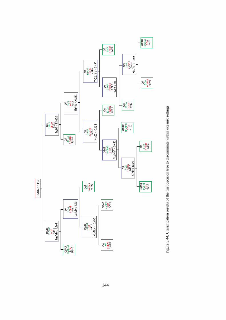
144
Figure 3.44. Classification results of the first decision tree to discriminate within oceanic settings
Fig
ure
3.4
4.
Cla
ssif
icat
ion
res
ult
s of
the
firs
t d
ecis
ion
tre
e to
dis
crim
inat
e w
ith
in o
cean
ic s
etti
ng
s
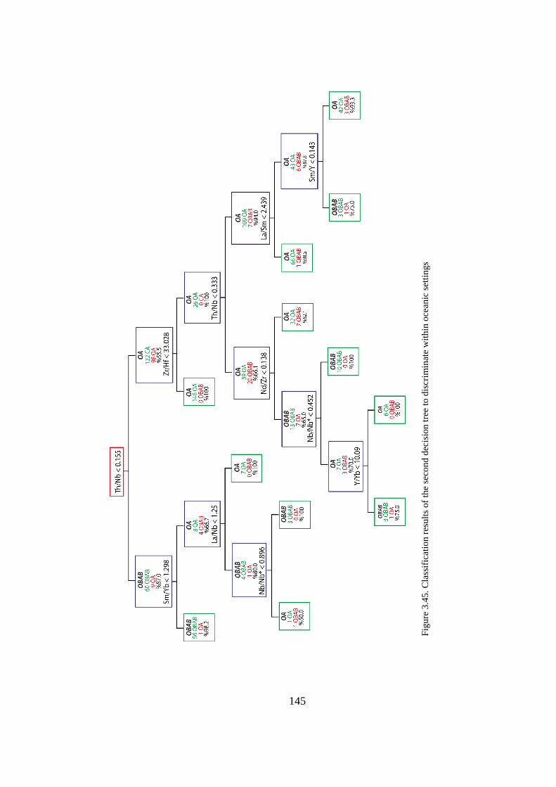
145
Figure 3.45. Classification results of the second decision tree to discriminate within oceanic settings
Fig
ure
3.4
5.
Cla
ssif
icat
ion
res
ult
s of
the
seco
nd
dec
isio
n t
ree
to d
iscr
imin
ate
wit
hin
oce
anic
set
tin
gs
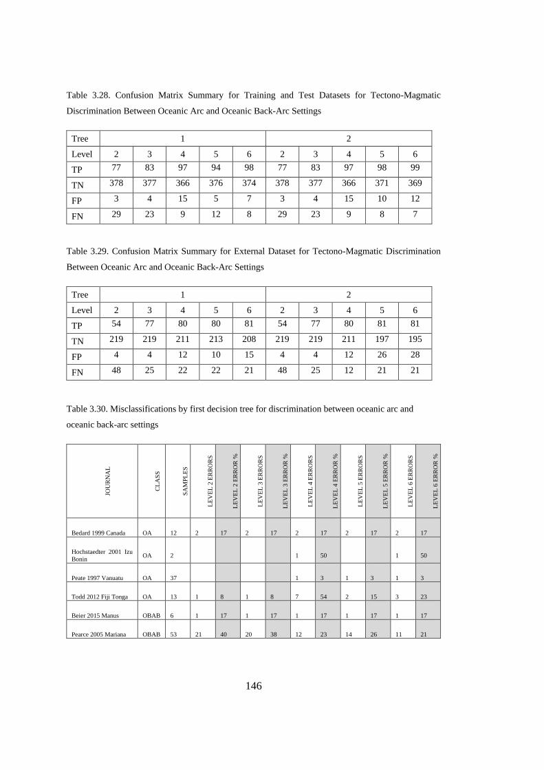
146
Table 3.28. Confusion Matrix Summary for Training and Test Datasets for Tectono-Magmatic
Discrimination Between Oceanic Arc and Oceanic Back-Arc Settings
Tree 1 2
Level 2 3 4 5 6 2 3 4 5 6
TP 77 83 97 94 98 77 83 97 98 99
TN 378 377 366 376 374 378 377 366 371 369
FP 3 4 15 5 7 3 4 15 10 12
FN 29 23 9 12 8 29 23 9 8 7
Table 3.29. Confusion Matrix Summary for External Dataset for Tectono-Magmatic Discrimination
Between Oceanic Arc and Oceanic Back-Arc Settings
Tree 1 2
Level 2 3 4 5 6 2 3 4 5 6
TP 54 77 80 80 81 54 77 80 81 81
TN 219 219 211 213 208 219 219 211 197 195
FP 4 4 12 10 15 4 4 12 26 28
FN 48 25 22 22 21 48 25 12 21 21
Table 3.30. Misclassifications by first decision tree for discrimination between oceanic arc and
oceanic back-arc settings
JOU
RN
AL
CL
AS
S
SA
MP
LE
S
LE
VE
L 2
ER
RO
RS
LE
VE
L 2
ER
RO
R %
LE
VE
L 3
ER
RO
RS
LE
VE
L 3
ER
RO
R %
LE
VE
L 4
ER
RO
RS
LE
VE
L 4
ER
RO
R %
LE
VE
L 5
ER
RO
RS
LE
VE
L 5
ER
RO
R %
LE
VE
L 6
ER
RO
RS
LE
VE
L 6
ER
RO
R %
Bedard 1999 Canada OA 12 2 17 2 17 2 17 2 17 2 17
Hochstaedter 2001 Izu
Bonin OA 2 1 50 1 50
Peate 1997 Vanuatu OA 37 1 3 1 3 1 3
Todd 2012 Fiji Tonga OA 13 1 8 1 8 7 54 2 15 3 23
Beier 2015 Manus OBAB 6 1 17 1 17 1 17 1 17 1 17
Pearce 2005 Mariana OBAB 53 21 40 20 38 12 23 14 26 11 21

147
Table 3.31. Misclassifications by first decision tree for discrimination between oceanic arc and
oceanic back-arc settings
JOU
RN
AL
CL
AS
S
SA
MP
LE
S
LE
VE
L 2
ER
RO
RS
LE
VE
L 2
ER
RO
R %
LE
VE
L 3
ER
RO
RS
LE
VE
L 3
ER
RO
R %
LE
VE
L 4
ER
RO
RS
LE
VE
L 4
ER
RO
R %
LE
VE
L 5
ER
RO
RS
LE
VE
L 5
ER
RO
R %
LE
VE
L 6
ER
RO
RS
LE
VE
L 6
ER
RO
R %
König 2008 Subduction OA 6 1 17 1 17 1 17 1 17 1 17
Pearce 1999 W. Pacific OA 5 1 20 1 20 2 40
Straub 2010 Izu Bonin OA 48 2 4 2 4 3 6 2 4 5 10
Tamura 2011 Mariana OA 19 4 21 4 21 4 21
Wharton 1994 Viti Levu OA 6 2 33 1 17 2 33
Woodhead 2001 Mixed OA 23 1 4 1 4 1 4 1 4 1 4
Ikeda 2016 Mariana OBAB 15 5 33 5 33 5 33 5 33 5 33
Ishizuka 2009 Izu Bonin OBAB 30 24 80 9 30 7 23 7 23 6 20
Mortimer 2007 South Fiji OBAB 12 8 67 5 42 4 33 4 33 4 33
Sinton 2003 Manus OBAB 6 6 100 6 100 6 100 6 100 6 100
Table 3.32. Misclassifications by second decision tree for discrimination between oceanic arc and
oceanic back-arc settings
JOU
RN
AL
CL
AS
S
SA
MP
LE
S
LE
VE
L 2
ER
RO
RS
LE
VE
L 2
ER
RO
R %
LE
VE
L 3
ER
RO
RS
LE
VE
L 3
ER
RO
R %
LE
VE
L 4
ER
RO
RS
LE
VE
L 4
ER
RO
R %
LE
VE
L 5
ER
RO
RS
LE
VE
L 5
ER
RO
R %
LE
VE
L 6
ER
RO
RS
LE
VE
L 6
ER
RO
R %
Bedard 1999 Canada OA 12 2 17 2 17 2 17 3 25 3 25
Hochstaedter 2001 Izu Bonin OA 2 1 50 1 50
Jolly 2007 Greater Antilles Arc OA 37 1 3 3 8 3 8
Jolly 2008 Greater Antilles Arc A OA 98 1 1 1 1 1 1 1 1
Peate 1997 Vanuatu OA 37 1 3 1 3 1 3
Todd 2012 Fiji Tonga OA 13 1 8 1 8 7 54 2 15 3 23
Beier 2015 Manus Basin OBAB 6 1 17 1 17 1 17 1 17 1 17
Pearce 2005 Mariana OBAB 53 21 40 20 38 12 23 11 21 9 17
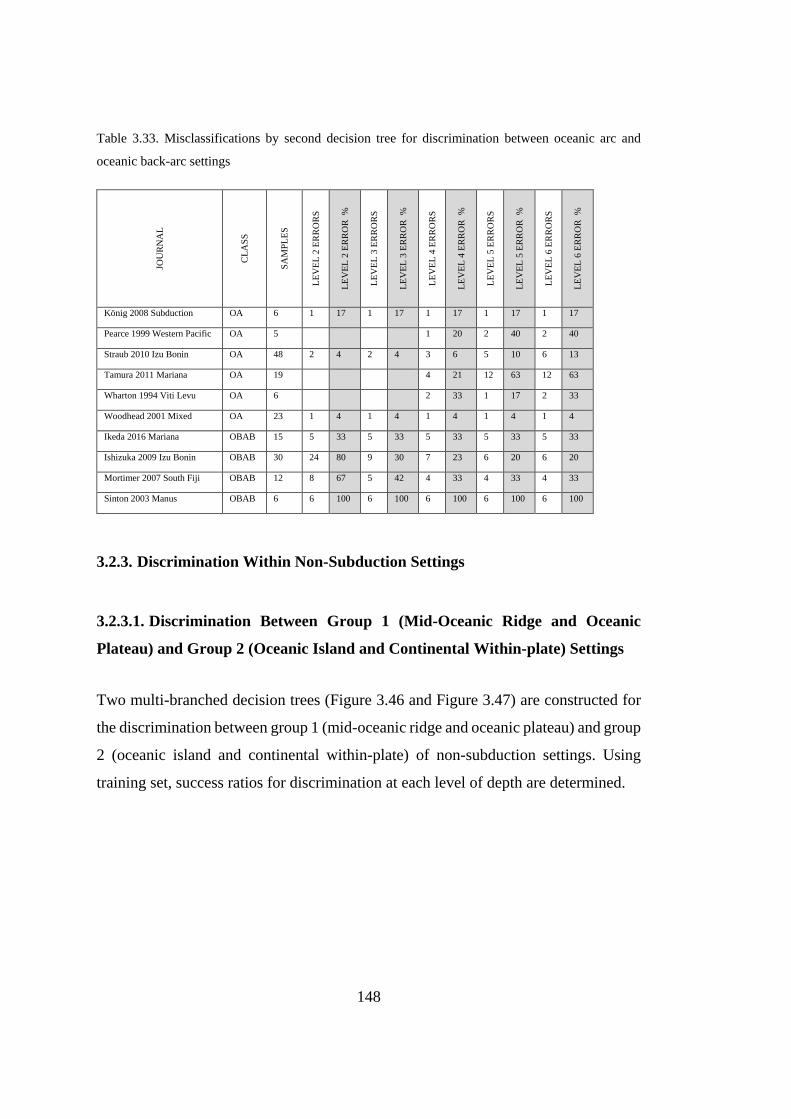
148
Table 3.33. Misclassifications by second decision tree for discrimination between oceanic arc and
oceanic back-arc settings JO
UR
NA
L
CL
AS
S
SA
MP
LE
S
LE
VE
L 2
ER
RO
RS
LE
VE
L 2
ER
RO
R %
LE
VE
L 3
ER
RO
RS
LE
VE
L 3
ER
RO
R %
LE
VE
L 4
ER
RO
RS
LE
VE
L 4
ER
RO
R %
LE
VE
L 5
ER
RO
RS
LE
VE
L 5
ER
RO
R %
LE
VE
L 6
ER
RO
RS
LE
VE
L 6
ER
RO
R %
König 2008 Subduction OA 6 1 17 1 17 1 17 1 17 1 17
Pearce 1999 Western Pacific OA 5 1 20 2 40 2 40
Straub 2010 Izu Bonin OA 48 2 4 2 4 3 6 5 10 6 13
Tamura 2011 Mariana OA 19 4 21 12 63 12 63
Wharton 1994 Viti Levu OA 6 2 33 1 17 2 33
Woodhead 2001 Mixed OA 23 1 4 1 4 1 4 1 4 1 4
Ikeda 2016 Mariana OBAB 15 5 33 5 33 5 33 5 33 5 33
Ishizuka 2009 Izu Bonin OBAB 30 24 80 9 30 7 23 6 20 6 20
Mortimer 2007 South Fiji OBAB 12 8 67 5 42 4 33 4 33 4 33
Sinton 2003 Manus OBAB 6 6 100 6 100 6 100 6 100 6 100
3.2.3. Discrimination Within Non-Subduction Settings
3.2.3.1. Discrimination Between Group 1 (Mid-Oceanic Ridge and Oceanic
Plateau) and Group 2 (Oceanic Island and Continental Within-plate) Settings
Two multi-branched decision trees (Figure 3.46 and Figure 3.47) are constructed for
the discrimination between group 1 (mid-oceanic ridge and oceanic plateau) and group
2 (oceanic island and continental within-plate) of non-subduction settings. Using
training set, success ratios for discrimination at each level of depth are determined.
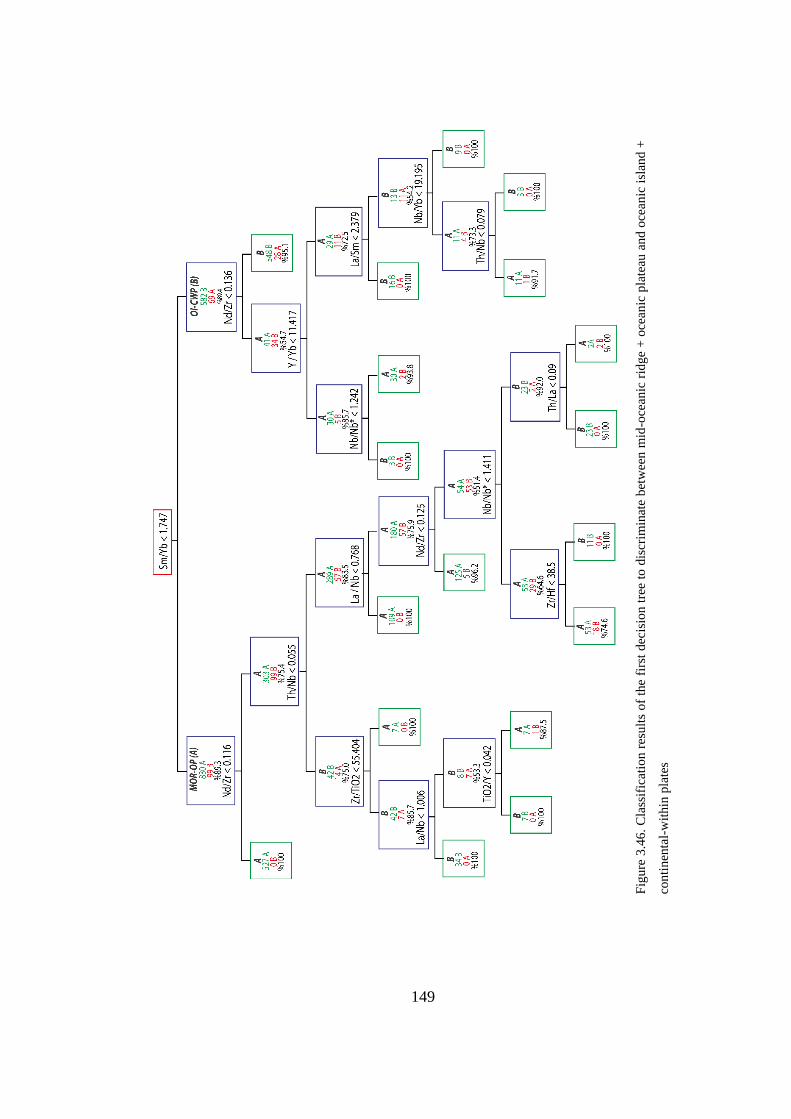
149
Figure 3.46. Classification results of the first decision tree to discriminate between mid-oceanic ridge + oceanic plateau and oceanic island +
continental-within plates
Fig
ure
3.4
6.
Cla
ssif
icat
ion
res
ult
s o
f th
e fi
rst
dec
isio
n t
ree
to d
iscr
imin
ate
bet
wee
n m
id-o
cean
ic r
idg
e +
oce
anic
pla
teau
an
d o
cean
ic i
slan
d +
con
tinen
tal-
wit
hin
pla
tes
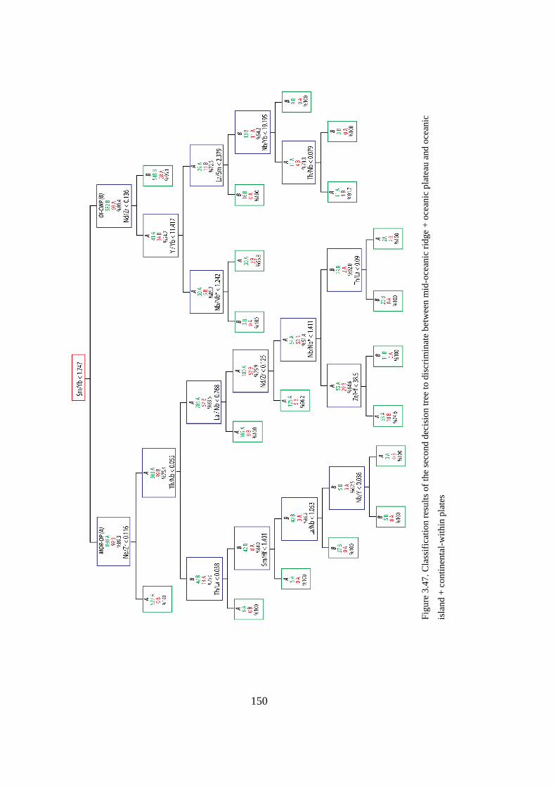
150
Figure 3.48. Classification results of the second decision tree to discriminate between mid-oceanic ridge + oceanic plateau and oceanic island + continental-within plates
Fig
ure
3.4
7.
Cla
ssif
icat
ion
res
ult
s of
the
seco
nd
dec
isio
n t
ree
to d
iscr
imin
ate
bet
wee
n m
id-o
cean
ic r
idg
e +
oce
anic
pla
teau
an
d o
cean
ic
isla
nd
+ c
onti
nen
tal-
wit
hin
pla
tes
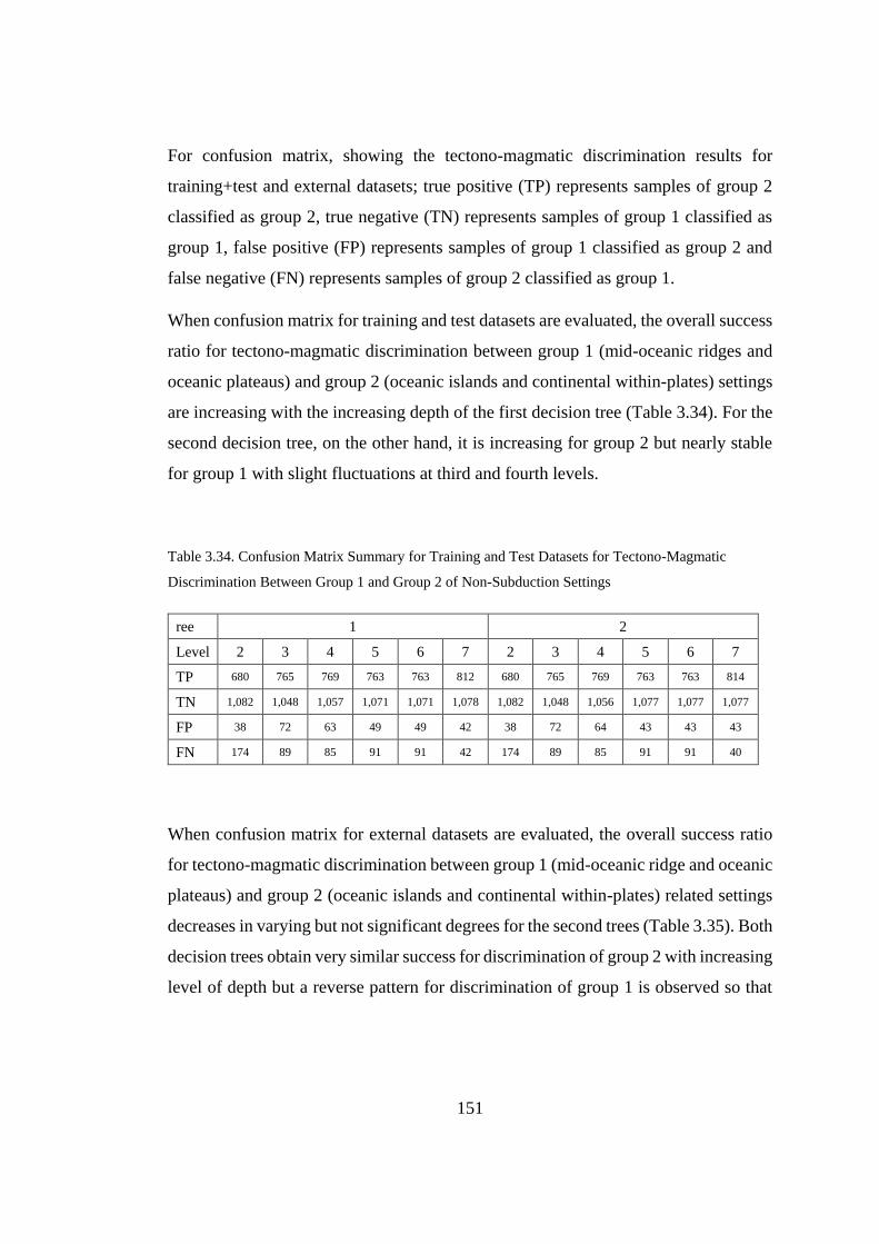
151
For confusion matrix, showing the tectono-magmatic discrimination results for
training+test and external datasets; true positive (TP) represents samples of group 2
classified as group 2, true negative (TN) represents samples of group 1 classified as
group 1, false positive (FP) represents samples of group 1 classified as group 2 and
false negative (FN) represents samples of group 2 classified as group 1.
When confusion matrix for training and test datasets are evaluated, the overall success
ratio for tectono-magmatic discrimination between group 1 (mid-oceanic ridges and
oceanic plateaus) and group 2 (oceanic islands and continental within-plates) settings
are increasing with the increasing depth of the first decision tree (Table 3.34). For the
second decision tree, on the other hand, it is increasing for group 2 but nearly stable
for group 1 with slight fluctuations at third and fourth levels.
Table 3.34. Confusion Matrix Summary for Training and Test Datasets for Tectono-Magmatic
Discrimination Between Group 1 and Group 2 of Non-Subduction Settings
ree 1 2
Level 2 3 4 5 6 7 2 3 4 5 6 7
TP 680 765 769 763 763 812 680 765 769 763 763 814
TN 1,082 1,048 1,057 1,071 1,071 1,078 1,082 1,048 1,056 1,077 1,077 1,077
FP 38 72 63 49 49 42 38 72 64 43 43 43
FN 174 89 85 91 91 42 174 89 85 91 91 40
When confusion matrix for external datasets are evaluated, the overall success ratio
for tectono-magmatic discrimination between group 1 (mid-oceanic ridge and oceanic
plateaus) and group 2 (oceanic islands and continental within-plates) related settings
decreases in varying but not significant degrees for the second trees (Table 3.35). Both
decision trees obtain very similar success for discrimination of group 2 with increasing
level of depth but a reverse pattern for discrimination of group 1 is observed so that
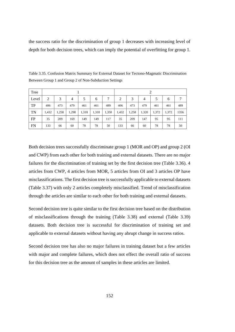
152
the success ratio for the discrimination of group 1 decreases with increasing level of
depth for both decision trees, which can imply the potential of overfitting for group 1.
Table 3.35. Confusion Matrix Summary for External Dataset for Tectono-Magmatic Discrimination
Between Group 1 and Group 2 of Non-Subduction Settings
Tree 1 2
Level 2 3 4 5 6 7 2 3 4 5 6 7
TP 406 473 479 461 461 489 406 473 479 461 461 489
TN 1,432 1,258 1,298 1,318 1,318 1,350 1,432 1,258 1,320 1,372 1,372 1356
FP 35 209 169 149 149 117 35 209 147 95 95 111
FN 133 66 60 78 78 50 133 66 60 78 78 50
Both decision trees successfully discriminate group 1 (MOR and OP) and group 2 (OI
and CWP) from each other for both training and external datasets. There are no major
failures for the discrimination of training set by the first decision tree (Table 3.36). 4
articles from CWP, 4 articles from MOR, 5 articles from OI and 3 articles OP have
misclassifications. The first decision tree is successfully applicable to external datasets
(Table 3.37) with only 2 articles completely misclassified. Trend of misclassification
through the articles are similar to each other for both training and external datasets.
Second decision tree is quite similar to the first decision tree based on the distribution
of misclassifications through the training (Table 3.38) and external (Table 3.39)
datasets. Both decision tree is successful for discrimination of training set and
applicable to external datasets without having any abrupt change in success ratios.
Second decision tree has also no major failures in training dataset but a few articles
with major and complete failures, which does not effect the overall ratio of success
for this decision tree as the amount of samples in these articles are limited.
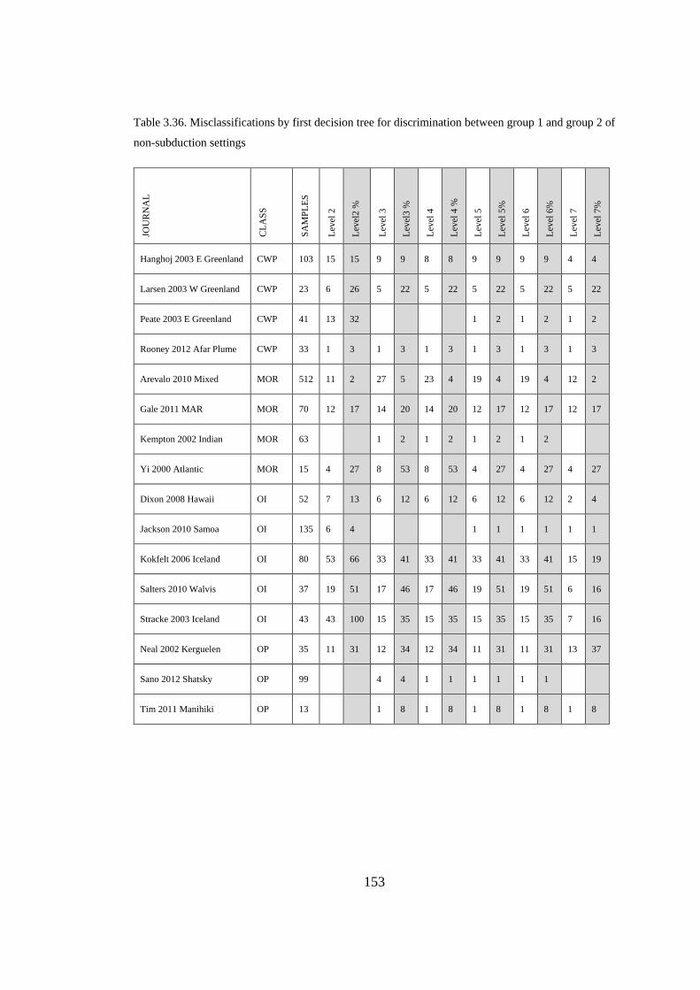
153
Table 3.36. Misclassifications by first decision tree for discrimination between group 1 and group 2 of
non-subduction settings JO
UR
NA
L
CL
AS
S
SA
MP
LE
S
Lev
el 2
Lev
el2
%
Lev
el 3
Lev
el3
%
Lev
el 4
Lev
el 4
%
Lev
el 5
Lev
el 5
%
Lev
el 6
Lev
el 6
%
Lev
el 7
Lev
el 7
%
Hanghoj 2003 E Greenland CWP 103 15 15 9 9 8 8 9 9 9 9 4 4
Larsen 2003 W Greenland CWP 23 6 26 5 22 5 22 5 22 5 22 5 22
Peate 2003 E Greenland CWP 41 13 32 1 2 1 2 1 2
Rooney 2012 Afar Plume CWP 33 1 3 1 3 1 3 1 3 1 3 1 3
Arevalo 2010 Mixed MOR 512 11 2 27 5 23 4 19 4 19 4 12 2
Gale 2011 MAR MOR 70 12 17 14 20 14 20 12 17 12 17 12 17
Kempton 2002 Indian MOR 63 1 2 1 2 1 2 1 2
Yi 2000 Atlantic MOR 15 4 27 8 53 8 53 4 27 4 27 4 27
Dixon 2008 Hawaii OI 52 7 13 6 12 6 12 6 12 6 12 2 4
Jackson 2010 Samoa OI 135 6 4 1 1 1 1 1 1
Kokfelt 2006 Iceland OI 80 53 66 33 41 33 41 33 41 33 41 15 19
Salters 2010 Walvis OI 37 19 51 17 46 17 46 19 51 19 51 6 16
Stracke 2003 Iceland OI 43 43 100 15 35 15 35 15 35 15 35 7 16
Neal 2002 Kerguelen OP 35 11 31 12 34 12 34 11 31 11 31 13 37
Sano 2012 Shatsky OP 99 4 4 1 1 1 1 1 1
Tim 2011 Manihiki OP 13 1 8 1 8 1 8 1 8 1 8

154
Table 3.37. Misclassifications by first decision tree for discrimination between group 1 and group 2 of
non-subduction settings
JOU
RN
AL
CL
AS
S
SA
MP
LE
S
Lev
el 2
Lev
el2
%
Lev
el 3
Lev
el3
%
Lev
el 4
Lev
el 4
%
Lev
el 5
Lev
el 5
%
Lev
el 6
Lev
el 6
%
Lev
el 7
Lev
el 7
%
Davies 2006 Aldan Shield CWP 7 1 14 1 14 1 14
Endress 2011 Egypt CWP 14 12 86 6 43 6 43 6 43
Frey 1996 Bunbury CWP 10 10 100 10 100 10 100 10 100 10 100 10 100
Furman 2006 Afar Plume CWP 37 2 5 1 3 1 3 2 5 2 5 2 5
Gibson 1995 SE Brazil CWP 32 1 3 1 3 1 3 1 3 1 3 1 3
Mana 2015 EAR CWP 29 2 7 1 3 1 3 1 3 1 3 1 3
Olierook 2016 Bunbury CWP 8 7 88 6 75 6 75 6 75 6 75 6 75
Shuying 2015 South China CWP 12 4 33 3 25 3 25 4 33 4 33 3 25
Xu 2001 SW China CWP 25 1 4 1 4 1 4 1 4 1 4 1 4
Jenner 2012 Mixed MOR 588 7 1 23 4 19 3 19 3 19 3 25 4
Kelley 2013 EPR MAR MOR 562 21 4 80 14 63 11 45 8 45 8 50 9
Zhang 2014 South Pacific MOR 118 72 61 48 41 48 41 48 41
Gibson 2005 Tristan OI 32 24 75 19 59 19 59 22 69 22 69 13 41
Kitagawa 2008 Iceland OI 107 35 33 17 16 17 16 22 21 22 21 12 11
Peate 2010 Iceland OI 18 2 11 1 6 1 6 2 11 2 11 1 6
Borisova 2002 Kerguelen OP 7 3 43 7 100 7 100 7 100 7 100 7 100
Frey 2002 Kerguelen OP 17 1 6 1 6 2 12 2 12 2 12 8 47
Shafer 2004 Ontong Java OP 10 1 10 1 10 1 10 1 10
Tejada 2002 Ontong Java OP 63 1 2 1 2 1 2 1 2 1 2
Trela 2015 Kerguelen OP 19 15 79 15 79 13 68 13 68 13 68
Weis 2002 Kerguelen OP 29 5 17 5 17 5 17 5 17

155
Table 3.38. Misclassifications by second decision tree for discrimination between group 1 and group
2 of non-subduction settings JO
UR
NA
L
CL
AS
S
SA
MP
LE
S
Lev
el 2
Lev
el2
%
Lev
el 3
Lev
el3
%
Lev
el 4
Lev
el 4
%
Lev
el 5
Lev
el 5
%
Lev
el 6
Lev
el 6
%
Lev
el 7
Lev
el 7
%
Hanghoj 2003 East
Greenland CWP 103 15 15 9 9 8 8 9 9 9 9 4 4
Larsen 2003 West
Greenland CWP 23 6 26 5 22 5 22 5 22 5 22 5 22
Peate 2003 East
Greenland CWP 41 13 32 1 2 1 2 1 2
Rooney 2012 Afar
Plume CWP 33 1 3 1 3 1 3 1 3 1 3 1 3
Arevalo 2010 Mixed MOR 512 11 2 27 5 21 4 15 3 15 3 13 3
Brandl 2012 EPR MOR 10 2 20 2 20
Gale 2011 MAR MOR 70 12 17 14 20 14 20 12 17 12 17 12 17
Yi 2000 Atlantic MOR 15 4 27 8 53 8 53 4 27 4 27 4 27
Dixon 2008 Hawaii OI 52 7 13 6 12 6 12 6 12 6 12 2 4
Jackson 2010 Samoa OI 135 6 4 1 1 1 1 1 1
Kokfelt 2006 Iceland OI 80 53 66 33 41 33 41 33 41 33 41 15 19
Salters 2010 Walvis OI 37 19 51 17 46 17 46 19 51 19 51 6 16
Stracke 2003 Iceland OI 43 43 100 15 35 15 35 15 35 15 35 5 12
Neal 2002 Kerguelen OP 35 11 31 12 34 12 34 11 31 11 31 13 37
Sano 2012 Shatsky OP 99 4 4 4 4 1 1 1 1
Tim 2011 Manihiki OP 13 1 8 1 8
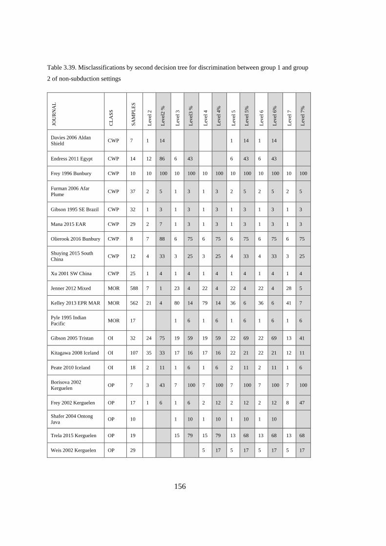
156
Table 3.39. Misclassifications by second decision tree for discrimination between group 1 and group
2 of non-subduction settings
JOU
RN
AL
CL
AS
S
SA
MP
LE
S
Lev
el 2
Lev
el2
%
Lev
el 3
Lev
el3
%
Lev
el 4
Lev
el 4
%
Lev
el 5
Lev
el 5
%
Lev
el 6
Lev
el 6
%
Lev
el 7
Lev
el 7
%
Davies 2006 Aldan
Shield CWP 7 1 14 1 14 1 14
Endress 2011 Egypt CWP 14 12 86 6 43 6 43 6 43
Frey 1996 Bunbury CWP 10 10 100 10 100 10 100 10 100 10 100 10 100
Furman 2006 Afar
Plume CWP 37 2 5 1 3 1 3 2 5 2 5 2 5
Gibson 1995 SE Brazil CWP 32 1 3 1 3 1 3 1 3 1 3 1 3
Mana 2015 EAR CWP 29 2 7 1 3 1 3 1 3 1 3 1 3
Olierook 2016 Bunbury CWP 8 7 88 6 75 6 75 6 75 6 75 6 75
Shuying 2015 South
China CWP 12 4 33 3 25 3 25 4 33 4 33 3 25
Xu 2001 SW China CWP 25 1 4 1 4 1 4 1 4 1 4 1 4
Jenner 2012 Mixed MOR 588 7 1 23 4 22 4 22 4 22 4 28 5
Kelley 2013 EPR MAR MOR 562 21 4 80 14 79 14 36 6 36 6 41 7
Pyle 1995 Indian
Pacific MOR 17 1 6 1 6 1 6 1 6 1 6
Gibson 2005 Tristan OI 32 24 75 19 59 19 59 22 69 22 69 13 41
Kitagawa 2008 Iceland OI 107 35 33 17 16 17 16 22 21 22 21 12 11
Peate 2010 Iceland OI 18 2 11 1 6 1 6 2 11 2 11 1 6
Borisova 2002
Kerguelen OP 7 3 43 7 100 7 100 7 100 7 100 7 100
Frey 2002 Kerguelen OP 17 1 6 1 6 2 12 2 12 2 12 8 47
Shafer 2004 Ontong
Java OP 10 1 10 1 10 1 10 1 10
Trela 2015 Kerguelen OP 19 15 79 15 79 13 68 13 68 13 68
Weis 2002 Kerguelen OP 29 5 17 5 17 5 17 5 17

157
3.2.3.2. Discrimination Between Mid-Oceanic Ridges and Oceanic Plateaus
Two multi-branched decision trees (Figure 3.48 and Figure 3.49) are constructed for
the discrimination between mid-oceanic ridge and oceanic plateau. Using training set,
success ratios for discrimination at each level of depth are determined.
For confusion matrix, showing the tectono-magmatic discrimination results for
training+test and external datasets; true positive (TP) represents samples of oceanic
plateaus classified as oceanic plateaus, true negative (TN) represents samples of mid-
oceanic ridges classified as mid-oceanic ridges, false positive (FP) represents samples
of mid-oceanic ridges classified as oceanic plateaus and false negative (FN) represents
samples of oceanic plateaus classified as mid-oceanic ridges.
When confusion matrix for training and test datasets are evaluated, the overall success
ratio for tectono-magmatic discrimination between mid-oceanic ridges and oceanic
plateaus are continuously increasing with the increasing level of depth in both decision
trees with a few exceptions (Table 3.40).
When confusion matrix for external datasets are evaluated, the overall success ratio
for tectono-magmatic discrimination between mid-oceanic ridges and oceanic
plateaus decreases in varying degrees for the second trees (Table 3.41).
The first decision tree is quite successful at the discrimination of MOR and OP for
training dataset, especially for samples of articles from MOR (Table 3.42). Only 1
article from MOR has misclassification and this is solved at sixth level.
The same success is also observed in external dataset with a similar trend for the
distribution of misclassification through the articles of MOR and OP (Table 3.43).
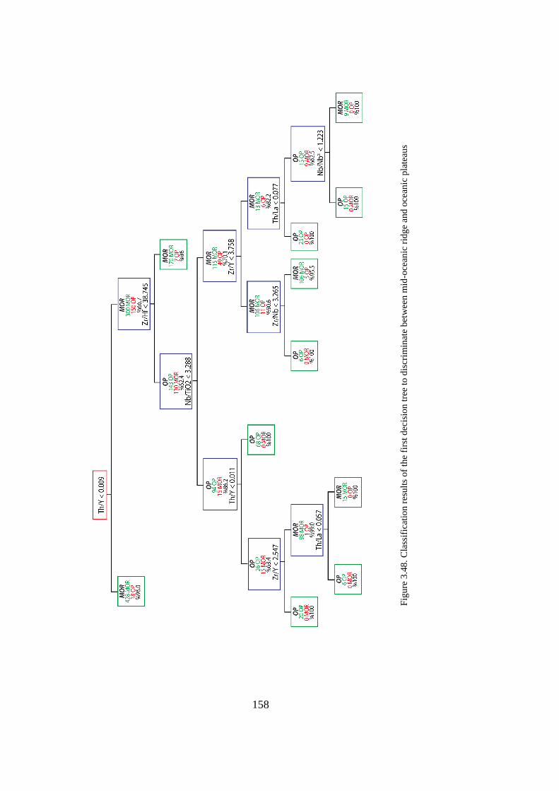
158
Figure 3.49. Classification results of the first decision tree to discriminate between mid-oceanic ridge and oceanic plateaus
Fig
ure
3.4
8.
Cla
ssif
icat
ion
res
ult
s of
the
firs
t dec
isio
n t
ree
to d
iscr
imin
ate
bet
wee
n m
id-o
cean
ic r
idg
e an
d o
cean
ic p
late
aus
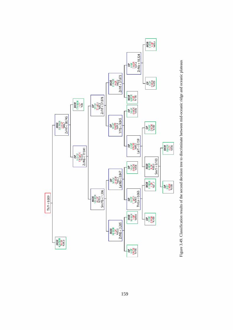
159
Figure 3.50. Classification results of the second decision tree to discriminate between mid-oceanic ridge and oceanic plateaus
Fig
ure
3.4
9.
Cla
ssif
icat
ion
res
ult
s of
the
seco
nd
dec
isio
n t
ree
to d
iscr
imin
ate
bet
wee
n m
id-o
cean
ic r
idg
e an
d o
cean
ic p
late
aus

160
Table 3.40. Confusion Matrix Summary for Training and Test Datasets for Tectono-Magmatic
Discrimination Between Mid-Oceanic Ridge and Oceanic Plateau Settings
Tree 1 2
Level 2 3 4 5 6 7 2 3 4 5 6 7
TP 176 118 162 159 167 167 176 121 161 175 175 171
TN 744 891 879 895 907 907 744 883 882 877 877 906
FP 165 18 30 14 2 2 165 26 27 32 32 3
FN 35 93 49 52 44 44 35 90 50 36 36 40
Table 3.41. Confusion Matrix Summary for External Dataset for Tectono-Magmatic Discrimination
Between Mid-Oceanic Ridge and Oceanic Plateaus
Tree 1 2
Level 2 3 4 5 6 2 3 4 5 6 7
TP 113 52 66 64 53 113 50 61 66 66 38
TN 966 1,236 1,206 1,252 1,277 966 1,210 1,217 1,188 1,188 1,270
FP 388 68 98 52 27 388 94 87 116 116 34
FN 50 111 97 99 110 50 113 102 97 97 125
The second decision tree is also quite similar to the first decision tree on the basis of
the success ratios and the distributions of misclassifications through the articles and
the tectonic settings.
It is quite successful at the discrimination of MOR and OP at training dataset (Table
3.44) and also applicable to external dataset (Table 3.45).
For both decision trees, MOR is much more successfully discriminated with respect
to OP and the trend of misclassifications through the articles in training set and
external dataset is similar to each other without any abrupt change in success ratio for
any specific articles or tectonic settings.
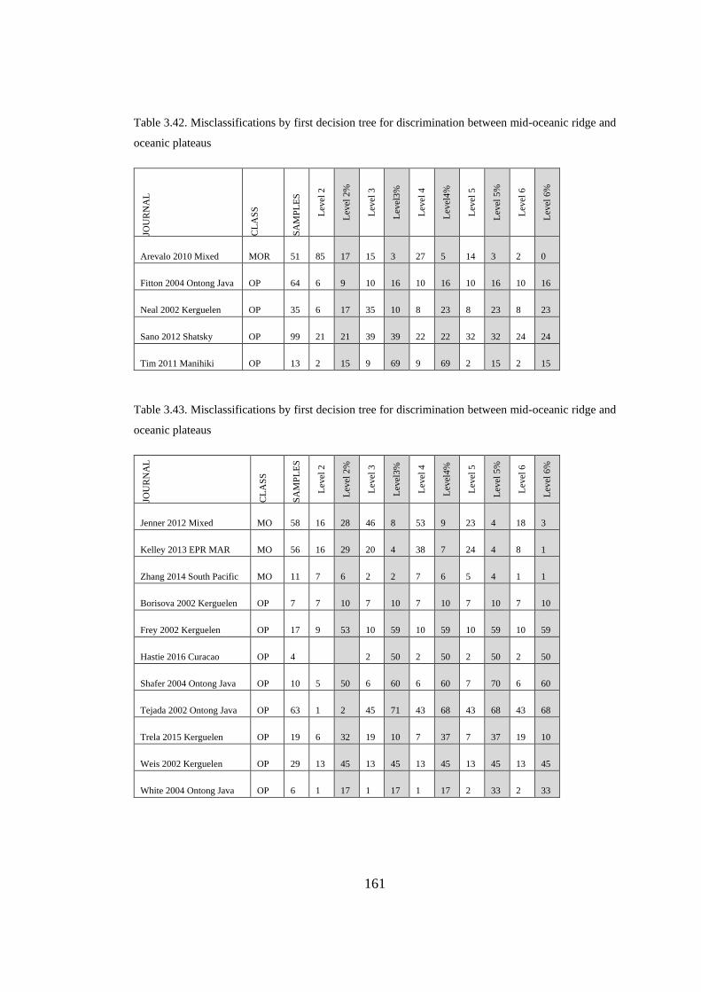
161
Table 3.42. Misclassifications by first decision tree for discrimination between mid-oceanic ridge and
oceanic plateaus JO
UR
NA
L
CL
AS
S
SA
MP
LE
S
Lev
el 2
Lev
el 2
%
Lev
el 3
Lev
el3
%
Lev
el 4
Lev
el4
%
Lev
el 5
Lev
el 5
%
Lev
el 6
Lev
el 6
%
Arevalo 2010 Mixed MOR 51
2
85 17 15 3 27 5 14 3 2 0
Fitton 2004 Ontong Java OP 64 6 9 10 16 10 16 10 16 10 16
Neal 2002 Kerguelen OP 35 6 17 35 10
0
8 23 8 23 8 23
Sano 2012 Shatsky OP 99 21 21 39 39 22 22 32 32 24 24
Tim 2011 Manihiki OP 13 2 15 9 69 9 69 2 15 2 15
Table 3.43. Misclassifications by first decision tree for discrimination between mid-oceanic ridge and
oceanic plateaus
JOU
RN
AL
CL
AS
S
SA
MP
LE
S
Lev
el 2
Lev
el 2
%
Lev
el 3
Lev
el3
%
Lev
el 4
Lev
el4
%
Lev
el 5
Lev
el 5
%
Lev
el 6
Lev
el 6
%
Jenner 2012 Mixed MO
R
58
8
16
6
28 46 8 53 9 23 4 18 3
Kelley 2013 EPR MAR MO
R
56
2
16
3
29 20 4 38 7 24 4 8 1
Zhang 2014 South Pacific MO
R
11
8
7 6 2 2 7 6 5 4 1 1
Borisova 2002 Kerguelen OP 7 7 10
0
7 10
0
7 10
0
7 10
0
7 10
0
Frey 2002 Kerguelen OP 17 9 53 10 59 10 59 10 59 10 59
Hastie 2016 Curacao OP 4 2 50 2 50 2 50 2 50
Shafer 2004 Ontong Java OP 10 5 50 6 60 6 60 7 70 6 60
Tejada 2002 Ontong Java OP 63 1 2 45 71 43 68 43 68 43 68
Trela 2015 Kerguelen OP 19 6 32 19 10
0
7 37 7 37 19 10
0
Weis 2002 Kerguelen OP 29 13 45 13 45 13 45 13 45 13 45
White 2004 Ontong Java OP 6 1 17 1 17 1 17 2 33 2 33

162
Table 3.44. Misclassifications by second decision tree for discrimination between mid-oceanic ridge
and oceanic plateaus
JOU
RN
AL
CL
AS
S
SA
MP
LE
S
Lev
el 2
Lev
el 2
%
Lev
el 3
Lev
el3
%
Lev
el 4
Lev
el4
%
Lev
el 5
Lev
el 5
%
Lev
el 6
Lev
el 6
%
Lev
el 7
Lev
el 7
%
Arevalo 2010 Mixed MOR 51
2
85 17 22 4 26 5 29 6 29 6 3 1
Gale 2011 MAR MOR 70 33 47 1 1 1 1 1 1
Nauret 2006 Central Indian MOR 34 5 15 2 6 1 3 1 3
Niu 1997 2002 EPR MOR 77 1 1 1 1 1 1 1 1
Fitton 2004 Ontong Java OP 64 6 9 8 13 12 19 7 11 7 11 7 11
Neal 2002 Kerguelen OP 35 6 17 35 10
0
6 17 6 17 6 17 6 17
Sano 2012 Shatsky OP 99 21 21 38 38 22 22 21 21 21 21 24 24
Tim 2011 Manihiki OP 13 2 15 9 69 10 77 2 15 2 15 3 23
Table 3.45. Misclassifications by second decision tree for discrimination between mid-oceanic ridge
and oceanic plateaus
JOU
RN
AL
CL
AS
S
SA
MP
LE
S
Lev
el 2
Lev
el 2
%
Lev
el 3
Lev
el3
%
Lev
el 4
Lev
el4
%
Lev
el 5
Lev
el 5
%
Lev
el 6
Lev
el 5
%
Lev
el 7
Lev
el 7
%
Jenner 2012 Mixed MOR 588 166 28 48 8 33 6 45 8 45 8 6 1
Kelley 2013 EPR MAR MOR 562 163 29 43 8 46 8 62 11 62 11 27 5
Pyle 1995 Indian Pacific MOR 17 2 12 1 6 1 6 2 12 2 12
Zhang 2014 South Pacific MOR 118 7 6 2 2 7 6 7 6 7 6 1 1
Borisova 2002 Kerguelen OP 7 7 100 7 100 7 100 7 100 7 100 7 100
Frey 2002 Kerguelen OP 17 9 53 16 94 15 88 14 82 14 82 14 82
Hastie 2016 Curacao OP 4 4 100 4 100 4 100 4 100 4 100
Shafer 2004 Ontong Java OP 10 5 50 6 60 6 60 6 60 6 60 8 80
Tejada 2002 Ontong Java OP 63 1 2 34 54 31 49 31 49 31 49 33 52
Trela 2015 Kerguelen OP 19 6 32 19 100 7 37 7 37 7 37 19 100
Weis 2002 Kerguelen OP 29 13 45 13 45 18 62 14 48 14 48 26 90
White 2004 Ontong Java OP 6 1 17 6 100 6 100 6 100 6 100 6 100

163
3.2.3.3. Discrimination Between Oceanic Islands and Continental Within-plates
Two multi-branched decision trees (Figure 3.50 and Figure 3.51) are constructed for
the discrimination between oceanic island and continental within-plates. Using
training set, success ratios for discrimination at each level of depth are determined.
For confusion matrix, showing the tectono-magmatic discrimination results for
training+test and external datasets; true positive (TP) represents samples of ocean
islands classified as ocean islands, true negative (TN) represents samples of
continental within-plates classified as continental within-plates, false positive (FP)
represents samples of continental within-plates classified as ocean islands and false
negative (FN) represents samples of ocean islands classified as continental within-
plates.
When confusion matrix for training and test datasets (Table 3.46) and external datasets
(Table 3.47) are evaluated, the overall success ratio for tectono-magmatic
discrimination between oceanic islands and continental within-plates are continuously
increasing with increasing level of depth in both decision trees. The success ratios for
the discrimination of both oceanic islands and continental within-plates reach their
maximum at the highest level of depth in both decision trees.
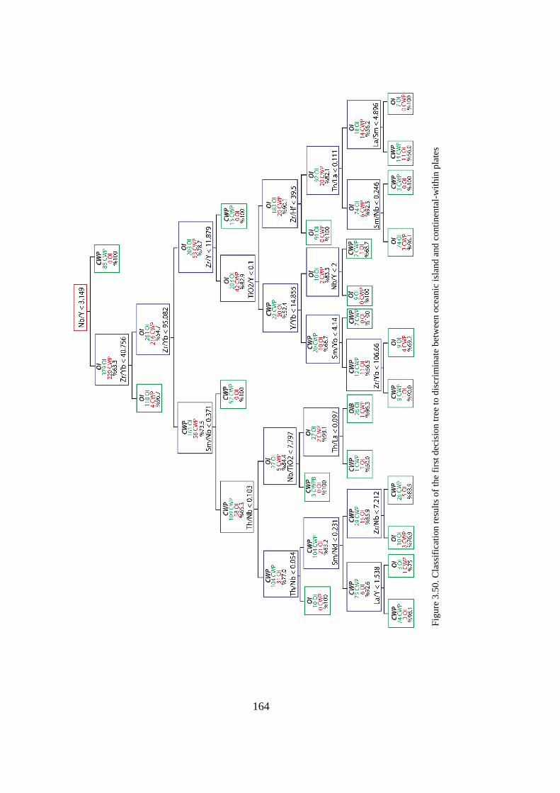
164
Figure 3.51. Classification results of the first decision tree to discriminate between oceanic island and continental-within plates
Fig
ure
3.5
0.
Cla
ssif
icat
ion
res
ult
s of
the
firs
t d
ecis
ion
tre
e to
dis
crim
inat
e b
etw
een
oce
anic
isl
and
and
co
nti
nen
tal-
wit
hin
pla
tes
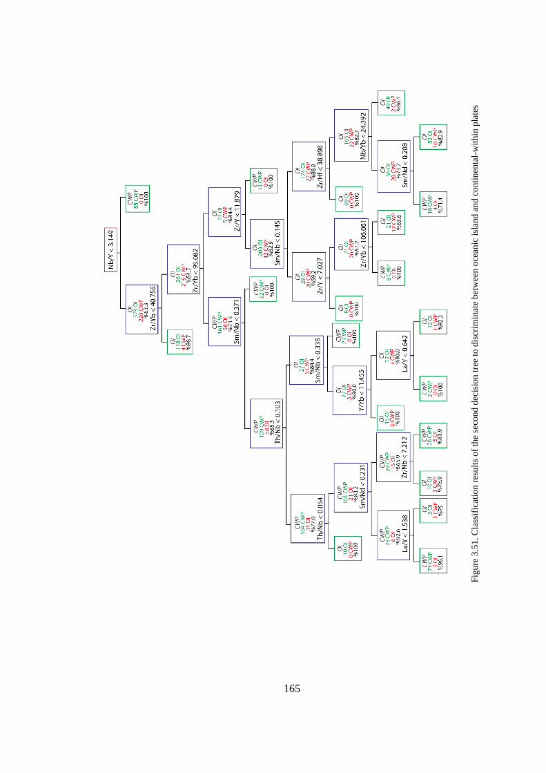
165
Figure 3.52. Classification results of the second decision tree to discriminate between oceanic island and continental-
within plates
Fig
ure
3.5
1.
Cla
ssif
icat
ion
res
ult
s of
the
seco
nd
dec
isio
n t
ree
to d
iscr
imin
ate
bet
wee
n o
cean
ic i
slan
d a
nd
co
nti
nen
tal-
wit
hin
pla
tes
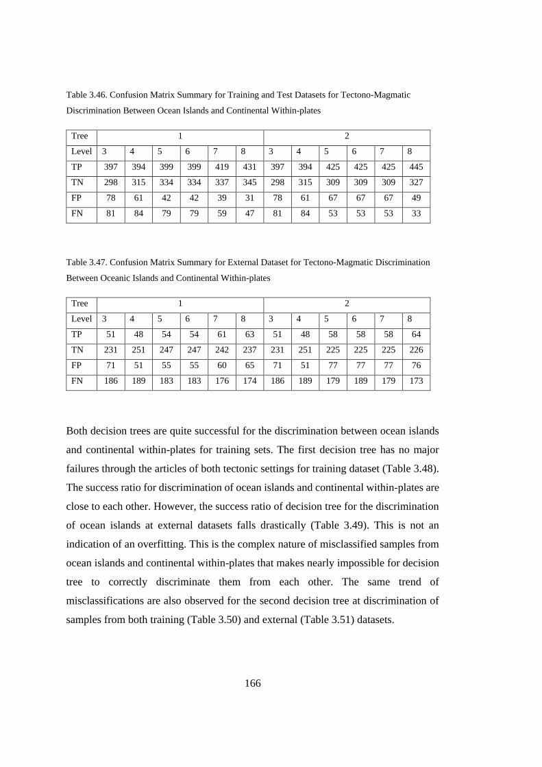
166
Table 3.46. Confusion Matrix Summary for Training and Test Datasets for Tectono-Magmatic
Discrimination Between Ocean Islands and Continental Within-plates
Tree 1 2
Level 3 4 5 6 7 8 3 4 5 6 7 8
TP 397 394 399 399 419 431 397 394 425 425 425 445
TN 298 315 334 334 337 345 298 315 309 309 309 327
FP 78 61 42 42 39 31 78 61 67 67 67 49
FN 81 84 79 79 59 47 81 84 53 53 53 33
Table 3.47. Confusion Matrix Summary for External Dataset for Tectono-Magmatic Discrimination
Between Oceanic Islands and Continental Within-plates
Tree 1 2
Level 3 4 5 6 7 8 3 4 5 6 7 8
TP 51 48 54 54 61 63 51 48 58 58 58 64
TN 231 251 247 247 242 237 231 251 225 225 225 226
FP 71 51 55 55 60 65 71 51 77 77 77 76
FN 186 189 183 183 176 174 186 189 179 189 179 173
Both decision trees are quite successful for the discrimination between ocean islands
and continental within-plates for training sets. The first decision tree has no major
failures through the articles of both tectonic settings for training dataset (Table 3.48).
The success ratio for discrimination of ocean islands and continental within-plates are
close to each other. However, the success ratio of decision tree for the discrimination
of ocean islands at external datasets falls drastically (Table 3.49). This is not an
indication of an overfitting. This is the complex nature of misclassified samples from
ocean islands and continental within-plates that makes nearly impossible for decision
tree to correctly discriminate them from each other. The same trend of
misclassifications are also observed for the second decision tree at discrimination of
samples from both training (Table 3.50) and external (Table 3.51) datasets.

167
Table 3.48. Misclassifications by first decision tree for discrimination between oceanic islands and
continental within-plates JO
UR
NA
L
CL
AS
S
SA
MP
LE
S
Lev
el 3
Lev
el 3
%
Lev
el 4
Lev
el4
%
Lev
el 5
Lev
el5
%
Lev
el 6
Lev
el6
%
Lev
el 7
Lev
el7
%
Lev
el 8
Lev
el8
%
Aviado 2015 West Antarctic CWP 19 12 63 12 63 5 26 5 26 5 26 6 32
Furman 2006 Turkana Kenya CWP 42 7 17 7 17 1 2 1 2 1 2 2 5
Gibson 2000 Picrite CWP 16 2 13 2 13 3 19 3 19 2 13
Hanghoj 2003 East Greenland CWP 10
3
11 11 11 11 11 11 11 11 8 8 8 8
Johnson 2005 Siberia CWP 18 15 83 15 83 9 50 9 50 10 56 2 11
Larsen 2003 West Greenland CWP 23 6 26 6 26 5 22 5 22 5 22 6 26
Peate 2003 East Greenland CWP 41 24 59 8 20 8 20 8 20 8 20 4 10
Rooney 2012 Afar Plume CWP 33 3 9
Dixon 2008 Hawaii OI 52 5 10 5 10 5 10 5 10 4 8 2 4
Geldmacher 2000 Madeira OI 49 7 14 8 16 14 29 14 29 14 29 6 12
Gurenko 2006 Canary OI 44 2 5 2 5 1 2
Jackson 2010 Samoa OI 13
5
9 7 11 8 12 9 12 9 12 9 16 12
Kokfelt 2006 Iceland OI 80 32 40 32 40 31 39 31 39 22 28 14 18
Millet 2009 Azores OI 21 1 5 1 5 3 14 3 14 3 14 2 10
Woodhead 1996 Mangaia OI 17 11 65 11 65 4 24 6 35
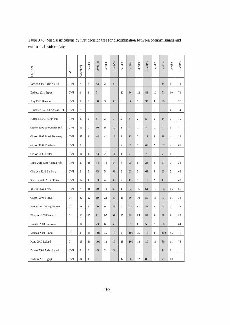
168
Table 3.49. Misclassifications by first decision tree for discrimination between oceanic islands and
continental within-plates
JOU
RN
AL
CL
AS
S
SA
MP
LE
S
Lev
el 3
Lev
el 3
%
Lev
el 4
Lev
el4
%
Lev
el 5
Lev
el5
%
Lev
el 6
Lev
el6
%
Lev
el 7
Lev
el7
%
Lev
el 8
Lev
el8
%
Davies 2006 Aldan Shield CWP 7 3 43 2 29 1 14 1 14
Endress 2011 Egypt CWP 14 1 7 12 86 12 86 10 71 10 71
Frey 1996 Bunbury CWP 10 3 30 3 30 3 30 3 30 3 30 3 30
Furman 2004 East African Rift CWP 29 1 3 4 14
Furman 2006 Afar Plume CWP 37 2 5 2 5 2 5 2 5 5 14 7 19
Gibson 1993 Rio Grande Rift CWP 15 9 60 9 60 1 7 1 7 1 7 1 7
Gibson 1995 Brazil Paraguay CWP 25 11 44 4 16 3 12 3 12 4 16 4 16
Gibson 1997 Trindade CWP 3 2 67 2 67 2 67 2 67
Gibson 2005 Tristan CWP 14 13 93 2 14 1 7 1 7 1 7 1 7
Mana 2015 East African Rift CWP 29 10 34 10 34 8 28 8 28 9 31 7 24
Olierook 2016 Bunbury CWP 8 5 63 5 63 5 63 5 63 5 63 5 63
Shuying 2015 South China CWP 12 4 33 4 33 2 17 2 17 2 17 5 42
Xu 2001 SW China CWP 25 10 40 10 40 16 64 16 64 16 64 15 60
Gibson 2005 Tristan OI 32 22 69 22 69 16 50 16 50 13 41 11 34
Hanyu 2011 Young Rurutu OI 21 6 29 9 43 9 43 9 43 9 43 9 43
Kitagawa 2008 Iceland OI 10
7
97 91 97 91 95 89 95 89 94 88 94 88
Lassiter 2003 Raivavae OI 14 6 43 6 43 8 57 8 57 7 50 9 64
Morgan 2009 Hawaii OI 45 45 100 45 10
0
45 100 45 10
0
45 100 45 10
0
Peate 2010 Iceland OI 18 18 100 18 10
0
18 100 18 10
0
16 89 14 78
Davies 2006 Aldan Shield CWP 7 3 43 2 29 1 14 1
Endress 2011 Egypt CWP 14 1 7 12 86 12 86 10 71 10
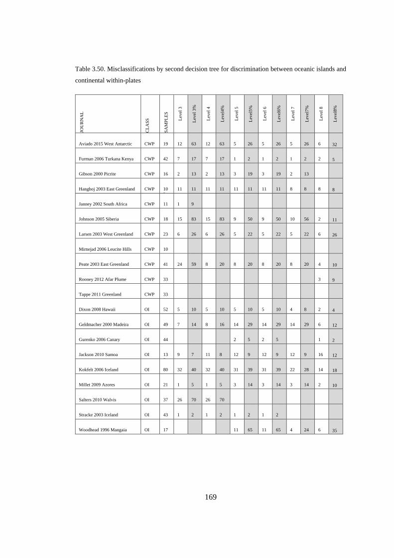
169
Table 3.50. Misclassifications by second decision tree for discrimination between oceanic islands and
continental within-plates JO
UR
NA
L
CL
AS
S
SA
MP
LE
S
Lev
el 3
Lev
el 3
%
Lev
el 4
Lev
el4
%
Lev
el 5
Lev
el5
%
Lev
el 6
Lev
el6
%
Lev
el 7
Lev
el7
%
Lev
el 8
Lev
el8
%
Aviado 2015 West Antarctic CWP 19 12 63 12 63 5 26 5 26 5 26 6 32
Furman 2006 Turkana Kenya CWP 42 7 17 7 17 1 2 1 2 1 2 2 5
Gibson 2000 Picrite CWP 16 2 13 2 13 3 19 3 19 2 13
Hanghoj 2003 East Greenland CWP 10
3
11 11 11 11 11 11 11 11 8 8 8 8
Janney 2002 South Africa CWP 11 1 9
Johnson 2005 Siberia CWP 18 15 83 15 83 9 50 9 50 10 56 2 11
Larsen 2003 West Greenland CWP 23 6 26 6 26 5 22 5 22 5 22 6 26
Mirnejad 2006 Leucite Hills CWP 10
Peate 2003 East Greenland CWP 41 24 59 8 20 8 20 8 20 8 20 4 10
Rooney 2012 Afar Plume CWP 33 3 9
Tappe 2011 Greenland CWP 33
Dixon 2008 Hawaii OI 52 5 10 5 10 5 10 5 10 4 8 2 4
Geldmacher 2000 Madeira OI 49 7 14 8 16 14 29 14 29 14 29 6 12
Gurenko 2006 Canary OI 44 2 5 2 5 1 2
Jackson 2010 Samoa OI 13
5
9 7 11 8 12 9 12 9 12 9 16 12
Kokfelt 2006 Iceland OI 80 32 40 32 40 31 39 31 39 22 28 14 18
Millet 2009 Azores OI 21 1 5 1 5 3 14 3 14 3 14 2 10
Salters 2010 Walvis OI 37 26 70 26 70
Stracke 2003 Iceland OI 43 1 2 1 2 1 2 1 2
Woodhead 1996 Mangaia OI 17 11 65 11 65 4 24 6 35
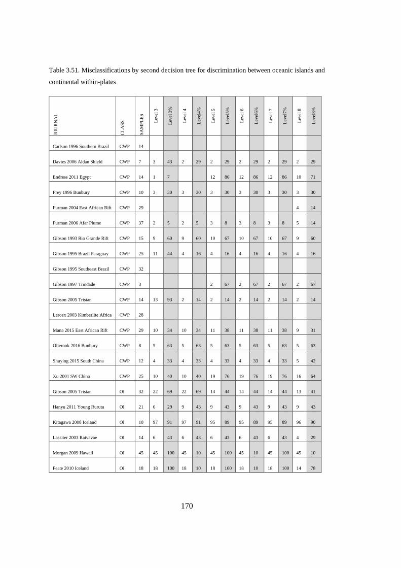
170
Table 3.51. Misclassifications by second decision tree for discrimination between oceanic islands and
continental within-plates
JOU
RN
AL
CL
AS
S
SA
MP
LE
S
Lev
el 3
Lev
el 3
%
Lev
el 4
Lev
el4
%
Lev
el 5
Lev
el5
%
Lev
el 6
Lev
el6
%
Lev
el 7
Lev
el7
%
Lev
el 8
Lev
el8
%
Carlson 1996 Southern Brazil CWP 14
Davies 2006 Aldan Shield CWP 7 3 43 2 29 2 29 2 29 2 29 2 29
Endress 2011 Egypt CWP 14 1 7 12 86 12 86 12 86 10 71
Frey 1996 Bunbury CWP 10 3 30 3 30 3 30 3 30 3 30 3 30
Furman 2004 East African Rift CWP 29 4 14
Furman 2006 Afar Plume CWP 37 2 5 2 5 3 8 3 8 3 8 5 14
Gibson 1993 Rio Grande Rift CWP 15 9 60 9 60 10 67 10 67 10 67 9 60
Gibson 1995 Brazil Paraguay CWP 25 11 44 4 16 4 16 4 16 4 16 4 16
Gibson 1995 Southeast Brazil CWP 32
Gibson 1997 Trindade CWP 3 2 67 2 67 2 67 2 67
Gibson 2005 Tristan CWP 14 13 93 2 14 2 14 2 14 2 14 2 14
Leroex 2003 Kimberlite Africa CWP 28
Mana 2015 East African Rift CWP 29 10 34 10 34 11 38 11 38 11 38 9 31
Olierook 2016 Bunbury CWP 8 5 63 5 63 5 63 5 63 5 63 5 63
Shuying 2015 South China CWP 12 4 33 4 33 4 33 4 33 4 33 5 42
Xu 2001 SW China CWP 25 10 40 10 40 19 76 19 76 19 76 16 64
Gibson 2005 Tristan OI 32 22 69 22 69 14 44 14 44 14 44 13 41
Hanyu 2011 Young Rurutu OI 21 6 29 9 43 9 43 9 43 9 43 9 43
Kitagawa 2008 Iceland OI 10
7 97 91 97 91 95 89 95 89 95 89 96 90
Lassiter 2003 Raivavae OI 14 6 43 6 43 6 43 6 43 6 43 4 29
Morgan 2009 Hawaii OI 45 45 100 45 10
0 45 100 45 10
0 45 100 45 10
0
Peate 2010 Iceland OI 18 18 100 18 10
0 18 100 18 10
0 18 100 14 78
171
CHAPTER 4
4. DISCUSSION
4.1. Discussion of Decision Trees
4.1.1. Discussion Based on Information Gain
Information gain is an important parameter for the selection of features in the
construction of decisin trees (Table 4.1). Element ratios with greater information gain
values are better discriminators and are preferred in decision trees.
Th/Nb and Nb/Nb* are useful discriminating features for discrimination between
subduction and non-subduction settings. Th and Nb behave as incompatible elements
during peridotitic upper mantle melting (e.g. Sun and McDonough, 1989). The
mineral phases in the mantle peridotite (olivine, clinopyroxene, orthopyroxene, spinel,
garnet) at these conditions are characterized by very low Dmelt/liquid; thus they have
only a minimal effect on the fractionation of Th/Nb. Their behavior, however, may
change significantly in subduction systems owing to dehydration and melting of the
slab and its mineralogy. During these processes, Th remains highly incompatible; it is
partitioned into the sediment melt and transferred into the mantle wedge (e.g. Elliott
et al., 1997). In contrast, Nb is retained in the slab, which is mainly linked to the
presence of Ti-bearing accessory phases, such as rutile (e.g. Ayers and Watson, 1993).
Thus, the transfer of Nb to the overlying mantle wedge is negligible. While the mantle
wedge remains pristine in terms of Nb (no addition), it becomes Th-rich with the flux
of this element via sediment melt. Therefore, during the subduction process, Th and
Nb are significantly fractioned, which causes the generation of magmas with high
Th/Nb signatures. It must also be noted that La (a LREE) displays somewhat a similar
behavior to Th since it is mobilized by slab-derived sediment melt. However, since Th
is relatively more incompatible than La, Th/Nb serves a more sensitive indicator of

172
the subduction component. The use of Nb/Nb* is due to the diverse behavior of Th
and La relative Nb, as explained before. Since the subduction-related magmas are
generally Th and La rich over Nb, they display negative anomalies. In this respect,
Nb/Nb* ratio is useful to see the magnitude of this relative depletion. In addition,
because of the integration of both Th and La at the same time, Nb/Nb* may act as a
better subduction indicator than Th/Nb.
Table 4.1. Information gain values of selected features for tectono-magmatic discriminations
Feature Sub
Nonsub
Arc
Backarc
OA
CA
Oceanic
Continental
OA
OBAB
MOR+OP
OI+CWP
MOR
OP
OI
CWP
La/Nb 0.445 0.166 0.149 0.128 0.208 0.108 0.112
La/Sm 0.086 0.378 0.052
La/Y 0.016 0.478 0.033 0.056
La/Yb 0.019 0.016 0.482
Nb/Nb* 0.550 0.203 0.079 0.093 0.262 0.010 0.030
Nb/TiO2 0.086 0.075
Nb/Y 0.147 0.029 0.424 0.078
Nb/Yb 0.019 0.460 0.077
Nd/TiO2 0.132 0.025 0.059
Nd/Zr 0.175 0.062 0.240 0.520
Sm/Hf 0.155 0.085 0.044 0.150
Sm/Nb 0.214 0.051
Sm/Nd 0.023 0.094
Sm/Y 0.147 0.039 0.042 0.165 0.118 0.148
Sm/Yb 0.150 0.477 0.105 0.097
Th/La 0.004 0.169 0.103 0.021
Th/Nb 0.528 0.196 0.253 0.087 0.042
Th/Y 0.019 0.162
Th/Yb 0.015 0.141
TiO2/Y 0.037 0.016 0.416 0.065
TiO2/Yb 0.115 0.035 0.480
Y/Yb 0.019 0.046 0.036 0.020 0.396 0.006 0.048
Zr/Hf 0.083 0.091 0.038 0.151 0.062 0.085 0.033
Zr/Nb 0.173 0.039 0.003 0.005 0.151
Zr/Sm 0.168 0.207
Zr/TiO2 0.166 0.141 0.055
Zr/Y 0.016 0.166 0.141 0.050 0.165
Zr/Yb 0.089 0.075 0.192

173
In contrast to Th/Nb and Nb/Nb*, which are used to assess the presence of the
subduction component, the role of Nb/Y and TiO2/Yb ratios are different. Nb, Ti, Y,
and Yb behave similarly during dehydration and melting of the slab; they are all
strongly conservative and retained in the slab (e.g. Pearce and Peate, 1995). Their
partitioning during the melting of mantle peridotite, however, is different. Nb is highly
incompatible, while Ti, Y, and Yb are all less incompatible than Nb (e.g. Sun and
McDonough, 1989). Thus, Nb/Y and TiO2/Yb can be fractionated under low degrees
of melting. In addition to melting, these ratios can also be controlled based on the
nature of the mantle source (depleted vs. enriched). For example, N-MORBs, which
are thought to be derived from depleted mantle sources (under moderate to high
degrees of melting), are characterized by low Nb/Y and TiO2/Yb ratios (e.g. Sun and
McDonough, 1989; Niu and Batiza, 1997; Hoernle et al., 2011). In contrast, enriched
magmas, such as E-MORBs and most OIBs, are characterized by high Nb/Y and
TiO2/Yb ratios, owing to the involvement of enriched sources and low-degree of
partial melting (e.g. Sun and McDonough, 1989; Chauvel et al., 1992; Workman et
al., 2004).
Furthermore, since melt extraction depletes the source more in Nb, the mantle source
domains that have previously experienced a melt extraction(s) is characterized by even
lower Nb/Y and TiO2/Yb ratios than those of N-MORBs (e.g. Pearce and Parkinson,
1993). This phenomenon is observed in some MORs and oceanic arcs, which seems
to have tapped pre-depleted mantle sources (e.g. Pearce et al., 1995; Niu and Batiza,
1997). Additionally, the presence of residual garnet can make a substantial effect on
Y and Yb, since these elements are strongly partitioned into garnet (e.g. McKenzie
and O’Nions, 1991). Therefore, melt generation involving garnet-bearing mantle
sources can result in magmas with high Nb/Y and TiO2/Yb ratios.
Although having relatively high information gain, gain ratio and gini index values,
Sm/Nb and Sm/Hf ratios are not preferred by any of the three decision trees at all.
174
For discrimination between arc and back-arc-related settings, the element ratios used
in these trees have relatively high information gain. However, features with high
information gain values (e.g. Th/Nb, La/Nb, and Sm/Y) are not preferred within two
decision trees constructed for discrimination of arc and back-arc-related settings.
In the classification of subduction-related settings, the Nd/Zr ratio appears as a new
ratio, not found in the previous discrimination. This element ratio contains trace
elements Nd and Zr, which display somewhat similar incompatibilities (e.g. Sun and
McDonough, 1989). Thus, except for the small degrees of partial melting, these
elements are expected not to fractionate significantly. However, a material like
sediment, which can be added to the mantle source of subduction zone magmas, may
cause a strong fractionation of this ratio. Sediments are known to be some distinct
geochemical features. For example, they are generally depleted in Zr (and Hf) relative
to Nd (and Sm) (e.g. Plank and Langmuir 1998). Thus, the addition of sediments with
high Nd/Zr ratios (e.g. via sediment melt) to the mantle source would directly affect
the composition of resulting magmas, leading to high Nd/Zr signatures.
For discrimination between OA and CA, the element ratios used in these trees have
relatively high information gain. However, Zr/Y having high information gain value
is not preferred within two decision trees constructed for discrimination of OA and
CA. In the discrimination between the oceanic and continental arcs, Zr/TiO2 and
Zr/Sm appear as the main discriminants. Regarding these pairs, Zr is relatively more
incompatible than both Ti and Sm (e.g. Sun and Donough, 1989). Zr and Ti are
subduction-immobile, while Sm is slightly subduction-mobile (Pearce and Peate
1995), thus it may cause some enrichment to some extent (though not much) in the
mantle wedge. Based on the partitioning behavior, the melts derived from depleted
sources under medium to high degrees of melting are characterized by lower Zr/TiO2
and Zr/Sm ratios (relative to the ones originated from enriched sources and/or by low
degrees of melting). Similarly, melt extraction would drive any mantle source domain
to lower values in both Zr/TiO2 and Zr/Sm. Sm/Y operates somewhat similarly to
Zr/TiO2 and Zr/Sm since Sm is more incompatible than Y. With increasing Zr/TiO2
175
and Zr/Sm, Sm/Y can also be expected to increase due to source enrichment and/or
decreasing degree of melting.
For discrimination between oceanic and continental settings, the element ratios used
in these trees have relatively high information gain. However, Zr/TiO2 having
maximum information gain value is not preferred within two decision trees. Zr/Y ratio
appears to be at the top discrimination between oceanic and continental subduction-
related settings. In this pair, both elements are subduction-immobile, thus unaffected
by the slab-derived contributions to the mantle wedge (e.g. Pearce and Stern 2006).
The operation of this ratio is somewhat similar to Zr/Sm and Zr/Ti, though the
incompatibility difference is more significant between Zr and Y (e.g. Sun and
McDonough, 1989). The source depletion would tend to lower Zr/Y ratio. In contrast,
decreasing degrees of partial melting would tend to increase this ratio.
Also, due to strong partitioning of Y into garnet, Zr/Y can be significantly
fractionated, if garnet remains as a residual mineral in the source; thus partial melting
processes involving garnet-bearing sources may have a substantial effect in the
fractionation of Zr/Y (particularly under low degrees of partial melting).
For discrimination between OA and OBAB, the element ratios used in these trees have
relatively high information gain. However, Zr/Sm having high information gain value
is not preferred within two decision trees constructed for discrimination of OA and
OBAB. The discrimination between oceanic arcs and back-arcs starts with Th/Nb,
which has been used also as a major feature in distinguishing between subduction and
non-subduction settings. Since the chemical behaviors of these elements are given
before, it is repeated here. However, in the discrimination of oceanic arcs and
backarcs, Zr/Hf seems to have involved at the upper levels, whose behavior deserves
some discussion. Zr and Hf are both subduction-immobile elements; thus their
contributions to the mantle wedge are negligible. Zr is slightly more incompatible than
Hf, which makes Zr to be concentrated more in the melt. Therefore, small degrees of
partial melting may produce magmas with relatively high Zr/Hf ratios when compared
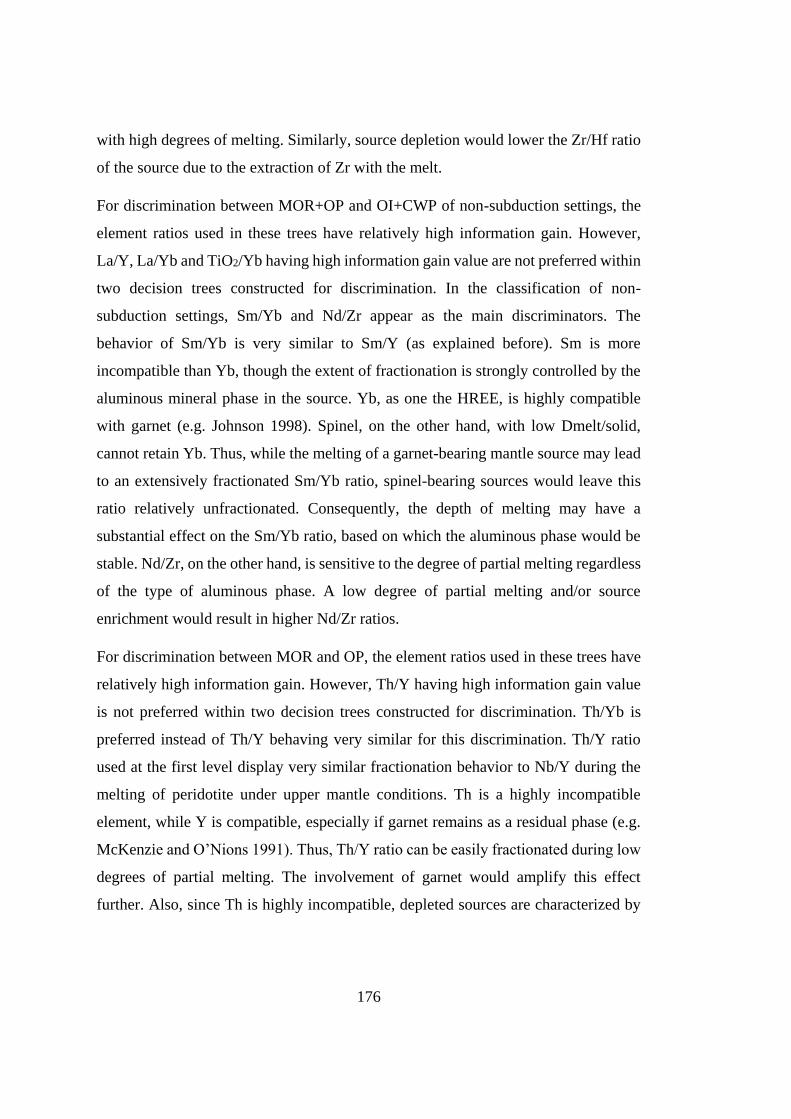
176
with high degrees of melting. Similarly, source depletion would lower the Zr/Hf ratio
of the source due to the extraction of Zr with the melt.
For discrimination between MOR+OP and OI+CWP of non-subduction settings, the
element ratios used in these trees have relatively high information gain. However,
La/Y, La/Yb and TiO2/Yb having high information gain value are not preferred within
two decision trees constructed for discrimination. In the classification of non-
subduction settings, Sm/Yb and Nd/Zr appear as the main discriminators. The
behavior of Sm/Yb is very similar to Sm/Y (as explained before). Sm is more
incompatible than Yb, though the extent of fractionation is strongly controlled by the
aluminous mineral phase in the source. Yb, as one the HREE, is highly compatible
with garnet (e.g. Johnson 1998). Spinel, on the other hand, with low Dmelt/solid,
cannot retain Yb. Thus, while the melting of a garnet-bearing mantle source may lead
to an extensively fractionated Sm/Yb ratio, spinel-bearing sources would leave this
ratio relatively unfractionated. Consequently, the depth of melting may have a
substantial effect on the Sm/Yb ratio, based on which the aluminous phase would be
stable. Nd/Zr, on the other hand, is sensitive to the degree of partial melting regardless
of the type of aluminous phase. A low degree of partial melting and/or source
enrichment would result in higher Nd/Zr ratios.
For discrimination between MOR and OP, the element ratios used in these trees have
relatively high information gain. However, Th/Y having high information gain value
is not preferred within two decision trees constructed for discrimination. Th/Yb is
preferred instead of Th/Y behaving very similar for this discrimination. Th/Y ratio
used at the first level display very similar fractionation behavior to Nb/Y during the
melting of peridotite under upper mantle conditions. Th is a highly incompatible
element, while Y is compatible, especially if garnet remains as a residual phase (e.g.
McKenzie and O’Nions 1991). Thus, Th/Y ratio can be easily fractionated during low
degrees of partial melting. The involvement of garnet would amplify this effect
further. Also, since Th is highly incompatible, depleted sources are characterized by
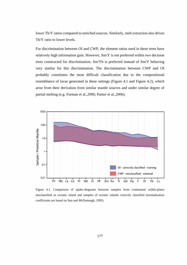
177
lower Th/Y ratios compared to enriched sources. Similarly, melt extraction also drives
Th/Y ratio to lower levels.
For discrimination between OI and CWP, the element ratios used in these trees have
relatively high information gain. However, Sm/Y is not preferred within two decision
trees constructed for discrimination. Sm/Yb is preferred instead of Sm/Y behaving
very similar for this discrimination. The discrimination between CWP and OI
probably constitutes the most difficult classification due to the compositional
resemblance of lavas generated in these settings (Figure 4.1 and Figure 4.2), which
arise from their derivation from similar mantle sources and under similar degree of
partial melting (e.g. Furman et al.,2006; Panter et al.,2006).
Figure 4.1. Comparison of spider-diagrams between samples from continental within-plates
misclassified as oceanic island and samples of oceanic islands correctly classified (normalization
coefficients are based on Sun and McDonough, 1995)

178
Since they include no or minimal subduction component in most cases, subduction-
sensitive ratios Th/Nb and Nb/Nb* do not work at the uppermost level. However,
some CWP lavas are result of very low degree of melting under great depths. These
ones, with potassic/ultrapotassic compositions, are extremely enriched in
incompatible elements (e.g. Janney et al.,2002). Thus, a ratio including a highly
incompatible element and compatible element that can be retained by garnet (like
Nb/Y) can be useful for the first order classification.
Figure 4.2. Comparison of spider-diagrams between samples oceanic islands misclassified as
continental within-plate and samples of continental within-plate correctly classified (normalization
coefficients are based on Sun and McDonough, 1995)
From information gain values of element ratios, it can be observed that the complexity
of discriminations increases towards the right side of the table as the effectiveness of
element ratios to discriminate settings decrease.
179
4.1.2. Discussion Based on Lift Curves and ROC Curves
When lift curves (Figure 4.3) are evaluated, it can be stated that most of the
classifications are constructed based on a model but not random. ROC curve of
decision trees (Figure 4.4) also indicates that the decision trees are successful with
high AUC values and classification ratios and developed based on a model having
AUC values greater than 0.5. Most of the classifications based on decision trees are
close to a wizard pattern, especially discrimination of
(1) OA-CA,
(2) Oceanic and continental settings,
(3) OA-OBAB,
(4) MOR+OP and OI+CWP, and
(5) OI-CWP.
Interestingly, decision trees for discrimination of MOR-OP and OI-CWP have
problems for the classification of external datasets by correct discrimination of OP,
OI and CWP. However, lift curve and ROC curves suggest that these
misclassifications are not based on the failure of decision tree models but based on the
characteristics of external samples and they can be inseparable due to several
geochemical or petrological constraints, which will be discussed and explained using
spider-diagrams.
4.1.3. Discussion Based on Statistical Evaluation of Decision Trees
Statistical parameters to consider the quality of decision trees are AUC (Area Under
ROC Curve), classification accuracy, f value, precision and recall values. When lift
curves and ROC are compared with area under ROC (AUC), classification accuracy,
f value, precision and recall values (Table 4.2, 4.3, 4.4, 4.5, 4.6, 4.7, 4.8 and 4.9),
nearly all decision trees have high AUC and classification accuracy values, which
indicates that they are constructed based on a model, which is successful in
discrimination of two settings as classes from each other.

180
Figure 4.3. Lift curve for tectonic discriminations

181
Figure 4.4. ROC for tectonic discriminations
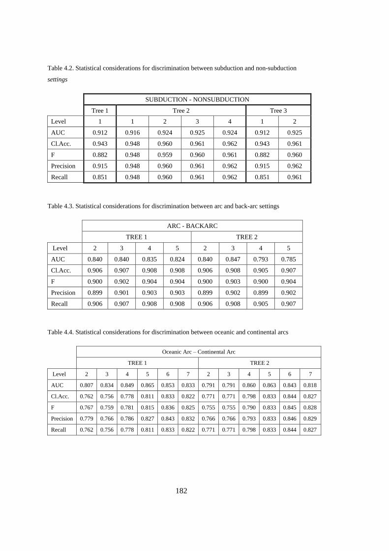
182
Table 4.2. Statistical considerations for discrimination between subduction and non-subduction
settings
SUBDUCTION - NONSUBDUCTION
Tree 1 Tree 2 Tree 3
Level 1 1 2 3 4 1 2
AUC 0.912 0.916 0.924 0.925 0.924 0.912 0.925
Cl.Acc. 0.943 0.948 0.960 0.961 0.962 0.943 0.961
F 0.882 0.948 0.959 0.960 0.961 0.882 0.960
Precision 0.915 0.948 0.960 0.961 0.962 0.915 0.962
Recall 0.851 0.948 0.960 0.961 0.962 0.851 0.961
Table 4.3. Statistical considerations for discrimination between arc and back-arc settings
ARC - BACKARC
TREE 1 TREE 2
Level 2 3 4 5 2 3 4 5
AUC 0.840 0.840 0.835 0.824 0.840 0.847 0.793 0.785
Cl.Acc. 0.906 0.907 0.908 0.908 0.906 0.908 0.905 0.907
F 0.900 0.902 0.904 0.904 0.900 0.903 0.900 0.904
Precision 0.899 0.901 0.903 0.903 0.899 0.902 0.899 0.902
Recall 0.906 0.907 0.908 0.908 0.906 0.908 0.905 0.907
Table 4.4. Statistical considerations for discrimination between oceanic and continental arcs
Oceanic Arc – Continental Arc
TREE 1 TREE 2
Level 2 3 4 5 6 7 2 3 4 5 6 7
AUC 0.807 0.834 0.849 0.865 0.853 0.833 0.791 0.791 0.860 0.863 0.843 0.818
Cl.Acc. 0.762 0.756 0.778 0.811 0.833 0.822 0.771 0.771 0.798 0.833 0.844 0.827
F 0.767 0.759 0.781 0.815 0.836 0.825 0.755 0.755 0.790 0.833 0.845 0.828
Precision 0.779 0.766 0.786 0.827 0.843 0.832 0.766 0.766 0.793 0.833 0.846 0.829
Recall 0.762 0.756 0.778 0.811 0.833 0.822 0.771 0.771 0.798 0.833 0.844 0.827
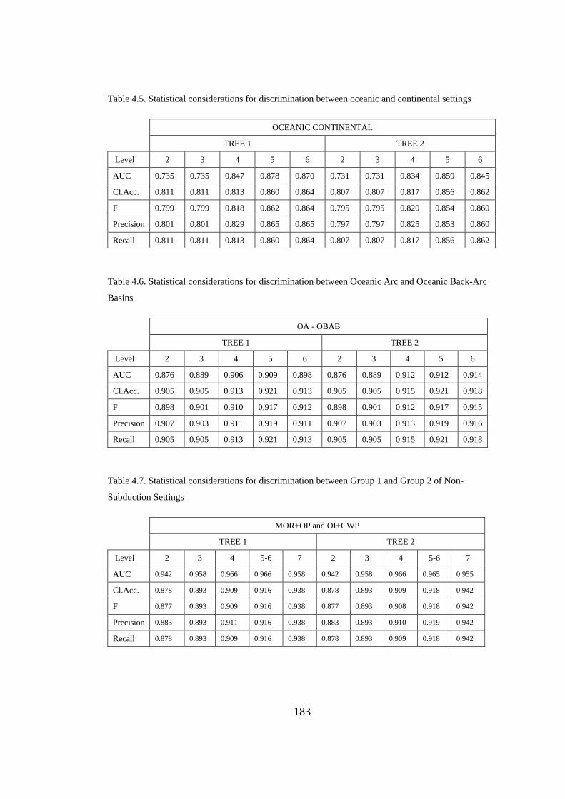
183
Table 4.5. Statistical considerations for discrimination between oceanic and continental settings
OCEANIC CONTINENTAL
TREE 1 TREE 2
Level 2 3 4 5 6 2 3 4 5 6
AUC 0.735 0.735 0.847 0.878 0.870 0.731 0.731 0.834 0.859 0.845
Cl.Acc. 0.811 0.811 0.813 0.860 0.864 0.807 0.807 0.817 0.856 0.862
F 0.799 0.799 0.818 0.862 0.864 0.795 0.795 0.820 0.854 0.860
Precision 0.801 0.801 0.829 0.865 0.865 0.797 0.797 0.825 0.853 0.860
Recall 0.811 0.811 0.813 0.860 0.864 0.807 0.807 0.817 0.856 0.862
Table 4.6. Statistical considerations for discrimination between Oceanic Arc and Oceanic Back-Arc
Basins
OA - OBAB
TREE 1 TREE 2
Level 2 3 4 5 6 2 3 4 5 6
AUC 0.876 0.889 0.906 0.909 0.898 0.876 0.889 0.912 0.912 0.914
Cl.Acc. 0.905 0.905 0.913 0.921 0.913 0.905 0.905 0.915 0.921 0.918
F 0.898 0.901 0.910 0.917 0.912 0.898 0.901 0.912 0.917 0.915
Precision 0.907 0.903 0.911 0.919 0.911 0.907 0.903 0.913 0.919 0.916
Recall 0.905 0.905 0.913 0.921 0.913 0.905 0.905 0.915 0.921 0.918
Table 4.7. Statistical considerations for discrimination between Group 1 and Group 2 of Non-
Subduction Settings
MOR+OP and OI+CWP
TREE 1 TREE 2
Level 2 3 4 5-6 7 2 3 4 5-6 7
AUC 0.942 0.958 0.966 0.966 0.958 0.942 0.958 0.966 0.965 0.955
Cl.Acc. 0.878 0.893 0.909 0.916 0.938 0.878 0.893 0.909 0.918 0.942
F 0.877 0.893 0.909 0.916 0.938 0.877 0.893 0.908 0.918 0.942
Precision 0.883 0.893 0.911 0.916 0.938 0.883 0.893 0.910 0.919 0.942
Recall 0.878 0.893 0.909 0.916 0.938 0.878 0.893 0.909 0.918 0.942

184
Table 4.8. Statistical considerations for discrimination between Mid-Ocean Ridge and Oceanic
Plateau
MID-OCEAN RIDGE - OCEANIC PLATEAU
TREE 1 TREE 2
Level 2 3 4 5 6 2 3 4 5 6 7
AUC 0.820 0.845 0.876 0.874 0.849 0.820 0.842 0.867 0.875 0.875 0.842
Cl.Acc. 0.825 0.879 0.925 0.924 0.934 0.825 0.868 0.921 0.922 0.922 0.934
F 0.836 0.868 0.924 0.921 0.931 0.836 0.853 0.919 0.920 0.920 0.932
Precision 0.857 0.872 0.923 0.922 0.933 0.857 0.859 0.918 0.919 0.919 0.932
Recall 0.825 0.879 0.925 0.924 0.934 0.825 0.868 0.921 0.922 0.922 0.934
Table 4.9. Statistical considerations for discrimination between Ocean Island and Continental Within-
Plate
OCEAN ISLAND - CONTINENTAL WITHIN-PLATE
TREE 1 TREE 2
Level 3 4 5-6 7 8 3 4 5-6-7 8
AUC 0.837 0.864 0.897 0.908 0.897 0.837 0.864 0.893 0.886
Cl.Acc. 0.807 0.827 0.851 0.870 0.863 0.807 0.827 0.961 0.855
F 0.807 0.828 0.851 0.870 0.862 0.807 0.828 0.861 0.855
Precision 0.807 0.828 0.851 0.870 0.862 0.807 0.828 0.862 0.855
Recall 0.807 0.827 0.851 0.870 0.863 0.807 0.827 0.861 0.855
4.2. Discussion of Classification Results
4.2.1. Discrimination Between Subduction and Non-Subduction Settings
For training and test datasets, the decision stump correctly classified 1,932 samples of
non-subduction out of 1,974 with a success ratio of 97.87% and 577 samples of
subduction out of 668 with a success rate of 86.38%. Decision stump using Th/Nb is

185
more effective for the tectono-magmatic discrimination of samples from non-
subduction settings compared to those from subduction settings.
The first decision tree is more successful than the decision stump at all levels. The
maximum classification ratio for samples of subduction settings is at levels 1, 3 and 4
with a success ratio of 88.47% (591 out of 668) and for samples of non-subduction
settings is at level 2 and 4 with a success ratio of 99.49% (1964 out of 1974). The
introduction of TiO2/Yb ratio to the second tree at the second level negatively affects
the correct classification of subduction samples with a decrease by 4 and the
introduction of Zr/Nb ratio to the second tree at the third level adversely affects the
correct classification of non-subduction samples with a decrease by 2.
The second decision tree is also more successful than the decision stump at all levels
except its first level for samples of non-subduction. The second decision tree has a
simple structure, which makes the application of this tree easier for users. This tree
has the same classification ratio of the second tree for the samples of subduction with
a success ratio of 88.47% (591 out of 668). However, for non-samples of non-
subduction, the second decision tree can only achieve the success ratio of the second
tree at its third level with a success ratio of 99.39% (1,962 out of 1,974). For the second
decision tree, the introduction of Nb/Y ratio at the second level has no effect on the
classification rate of subduction but has a positive impact on samples of non-
subduction with an increase by 34.
For external datasets, the decision stump has a correct classification ratio of 96.56%
for samples of non-subduction (1,937 out of 2006) and 80.47% for samples of
subduction (375 out of 466). Although success ratios decrease about 1% for non-
subduction and 6% for subduction, decision stump shall be accepted to be a successful
method to discriminate between subduction and non-subduction settings with a single
discriminating feature (Th/Nb).
The first decision tree has its maximum classification ratio at levels 1, 3, and 4 for
samples of subduction with a success ratio of 84.98% (396 out of 466) and level 2 for
186
samples of non-subduction with success ratio of 98.75% (1,981 out of 2,006). With
the introduction of Zr/Nb ratio at the third level of the second tree, the correct
classification for samples of non-subduction decreases by 4, and the introduction of
La/Nb ratio at the fourth level had no positive or negative effect relative to level 3.
The introduction of TiO2/Yb has a negligible negative impact on correct classification
for samples of subduction samples with a decrease by 1. The first decision tree is more
applicable to external datasets when compared to decision stump, although success
ratios decrease about 1% for non-subduction and 3% for subduction. Both level 2 for
its simplicity and level 4 for its maximum success ratio for both training-test and
external datasets shall be preferred.
The second decision tree is also more applicable to external datasets when compared
to decision stump along with a simple structure with only 2 levels in depth. This tree
has its maximum classification ratio at level 1 for samples of subduction with a success
ratio of 84.98% (396 out of 466) and level 2 for samples of non-subduction with
success ratio of 98.65% (1,979 out of 2,006). The introduction of Nb/Y has a slightly
negative effect on the correct classification of subduction with a decrease by 3 but a
considerable positive impact on that of non-subduction with an increase by 37.
Therefore, the overall success ratio of level 2 of the second decision tree is much better
than level 1. The success ratios for application of this decision tree to external datasets
decrease by about 1% for non-subduction and 4% for subduction.
The decision trump has only single level of depth using Th/Nb ratio (also known as
decision stump) obtained a very high success ratio for all datasets (more than 90% in
overall) and became more successful for samples of non-subduction with respect to
those of subduction eliminating the risk of underfitting due to its simple structure. The
success ratio of this decision tree is distributed homogeneously through the articles
from different locations, with a few exceptions for the training and test datasets.
For training and test datasets, 45 articles out of 63 having 2,045 samples are classified
correctly with 100% success ratio. 18 articles have misclassifications with varying
187
misclassification ratios. Mid-oceanic ridges are completely classified as “non-
subduction setting” with a 100% success ratio. Continental arcs, continental within-
plates, oceanic arcs, oceanic islands are quite successful for the discrimination
between subduction and non-subduction. Misclassifications for the decision stump are
only 6 samples of continental arcs out of 181 samples from 7 articles, 38 samples of
continental within-plates out of 376 samples from 12 articles, 16 samples of oceanic
arcs out of 381 samples from 14 articles and only 1 samples of oceanic islands out of
478 samples from 9 articles. For continental arcs, Mullen (2017) of Cascade Arcs is
the only article, having misclassifications with a misclassification ratio of 17.14% (6
out of 35). For continental within-plates, Mirnejad (2006) of Leucite Hills and Coe
(2008) of South Africa are misclassified as “subduction” by decision trump with
misclassification rates of 100% and 85.19%, with respectively. Gibson (2000) and
Janney (2002), on the other hand, obtained relatively high success ratios with low
misclassification rates.
For oceanic arcs, 6 articles have slight misclassification rates ranging from 1% to 38%:
Jolly (2008a), Tollstrup (2010), Pearce (2005), Jolly (2007), Bedard (1999) and Todd
(2012) with an order of increasing misclassification rate. Oceanic back-arcs generally
failed at discrimination between subduction and non-subduction settings. All 5 articles
have larger misclassification rates, with 4 of them having a misclassification rate
greater than 50%. Pearce (2005) almost completely failed with a misclassification rate
of 96% (24 out of 25 samples). Oceanic islands and oceanic plateaus are also quite
successful for the discrimination between subduction and non-subduction. Only 1
sample of oceanic island is misclassified out of 478 samples from 9 articles, and only
3 samples of oceanic plateaus are misclassified out of 211 samples from 4 articles.
The decision stump is also successfully applicable to the tectono-magmatic
discrimination of external datasets. For external datasets, 38 articles out of 62 having
1,406 samples are classified correctly with 100% success ratio. 24 articles have
misclassifications with varying misclassification ratios. Continental arcs and oceanic
islands are entirely classified with 100% success ratio. Mid-oceanic ridges and oceanic
188
plateaus are also quite successful for the discrimination between subduction and non-
subduction. Only 3 samples of mid-oceanic ridge are misclassified out of 1,304
samples from 5 articles, and only 2 samples are misclassified out of 163 samples from
9 articles. Oceanic back-arcs and continental within-plates generally failed at the
discrimination between subduction and non-subduction settings. For oceanic back-
arcs, 5 articles out of 6 completely failed for discrimination. For continental within-
plates, 9 articles out of 16 have misclassifications with rates ranging between 10% and
100%. Davies (2006) of Aldan Shield, Gibson (2005) of Tristan, and Oliebrook (2016)
of Bunbury failed for the discrimination almost completely. In spite of having
misclassifications in several articles for oceanic arcs, the only problematic one is
König (2008), with samples from various subduction zones with a misclassification
rate of 50%.
The first decision tree became more successful compared to the decision stump, and
misclassifications have a homogeneous distribution through the articles from different
locations for training and test datasets. For training and test datasets, 48 articles out of
63 having 1,674 samples are classified correctly with 100% success ratio. 15 articles
have misclassifications with varying misclassification ratios. Oceanic islands are
completely classified with 100% success ratio at all levels of this decision tree.
Continental arcs, mid-oceanic ridges, oceanic arcs and oceanic plateaus are also quite
successful for the discrimination between subduction and non-subduction.
Misclassifications for the second tree are only 6 samples of continental arcs out of 181
samples from 7 articles, 8 samples of mid-oceanic ridges out of 909 samples from 12
articles, 11 samples of oceanic arcs out of 381 samples from 14 articles and 1 sample
of oceanic plateau out of 211 samples from 4 articles.
The first decision tree is also much more effective for the discrimination of continental
within-plates when compared to decision stump with only 1 misclassification out of
376 samples from 12 articles. The problem in tectono-magmatic discrimination of
oceanic back-arcs can not be solved at the second tree. All articles from oceanic back-
arc have large amounts of misclassifications with ratios more than 50% except one

189
(24%). When different levels of this decision tree are evaluated, especially the
introduction of TiO2/Yb ratio at level 2 can correctly discriminate most of the
continental within-plates, that have been misclassified at level 1. However,
interestingly, increasing level of depth for the second decision tree seems to have no
positive or negative effect on the misclassifications at the first level. For such articles,
there is no apparent difference between level 1 and level 4. Therefore, levels 2, 3 and
4 shall be used for discrimination between subduction and non-subduction without
having a significant difference in their success ratios.
The first decision tree is also successfully applicable to the tectono-magmatic
discrimination of external datasets. For external datasets, 45 articles out of 62 having
1,055 samples are classified correctly with 100% success ratio. 17 articles have
misclassifications with varying misclassification ratios. Continental arcs, oceanic
islands, and oceanic plateaus are completely classified with 100% success ratio at all
levels of this decision tree. This result indicates that Nb/Nb* ratio is quite effective
discriminating feature for these three tectonic settings. Mid-oceanic ridges and
oceanic arcs are also quite successful for the discrimination between subduction and
non-subduction. Misclassifications for the second tree are only 9 samples of mid-
oceanic ridges out of 1,304 samples from 5 articles and 6 samples of oceanic arcs out
of 223 samples from 12 articles. The problem in tectono-magmatic discrimination of
continental within-plates and oceanic back-arcs can not be solved for the external
datasets at the second tree. Only Gibson (2005) of Tristan can be correctly classified
with the introduction of TiO2/Yb ratio at the second level. Other than the introduction
of TiO2/Yb ratio, increasing the level of depth in the second decision tree seems to
have no positive or negative effect for the articles misclassified at the first level.
Therefore, for external datasets, levels 2 and 4 of the first decision tree shall be used
for discrimination between subduction and non-subduction.

190
The second decision tree also became more successful compared to the decision stump
through articles from different locations in spite of having a simple structure when
compared with the first decision tree.
For training and test datasets, 47 articles out of 63 having 1,578 samples are classified
correctly with 100% success ratio. 16 articles have misclassifications with varying
misclassification ratios. Oceanic islands are completely classified with 100% success
ratio at all levels of this decision tree.
Continental arcs, mid-oceanic ridges, oceanic arcs, and oceanic plateaus are quite
successful for the discrimination between subduction and non-subduction.
Misclassifications for the second decision tree are only 6 samples of continental arcs
out of 181 samples from 7 articles, 8 samples of mid-oceanic ridges out of 909 samples
from 12 articles, 11 samples of oceanic arcs out of 381 samples from 14 articles and
1 sample of oceanic plateau out of 211 samples from 4 articles. Continental within-
plates cannot be correctly classified at the first level of this decision tree, but with the
introduction of Nb/Y ratio at the second level, only 3 samples are misclassified out of
376 samples from 12 articles. Oceanic back-arcs cannot be discriminated with the
second decision tree just like the other decision trees, so they are considered as
problematic.
The second decision tree is also successfully applicable for tectono-magmatic
discrimination of external datasets, just like to previous two decision trees. Among all
decision trees constructed for the tectono-magmatic discrimination between
subduction and non-subduction, no underfitting or overfitting has been observed.
For external datasets, 45 articles out of 62 having 1,055 samples are classified
correctly with 100% success ratio. 17 articles have misclassifications with varying
misclassification ratios. Oceanic islands and oceanic plateaus are completely
classified correctly with 100% success ratio at all levels of this decision tree.
Continental arcs are classified correctly at the first level, but with the addition of Nb/Y
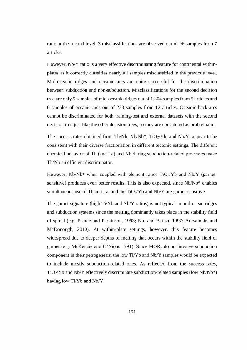
191
ratio at the second level, 3 misclassifications are observed out of 96 samples from 7
articles.
However, Nb/Y ratio is a very effective discriminating feature for continental within-
plates as it correctly classifies nearly all samples misclassified in the previous level.
Mid-oceanic ridges and oceanic arcs are quite successful for the discrimination
between subduction and non-subduction. Misclassifications for the second decision
tree are only 9 samples of mid-oceanic ridges out of 1,304 samples from 5 articles and
6 samples of oceanic arcs out of 223 samples from 12 articles. Oceanic back-arcs
cannot be discriminated for both training-test and external datasets with the second
decision tree just like the other decision trees, so they are considered as problematic.
The success rates obtained from Th/Nb, Nb/Nb*, TiO2/Yb, and Nb/Y, appear to be
consistent with their diverse fractionation in different tectonic settings. The different
chemical behavior of Th (and La) and Nb during subduction-related processes make
Th/Nb an efficient discriminator.
However, Nb/Nb* when coupled with element ratios TiO2/Yb and Nb/Y (garnet-
sensitive) produces even better results. This is also expected, since Nb/Nb* enables
simultaneous use of Th and La, and the TiO2/Yb and Nb/Y are garnet-sensitive.
The garnet signature (high Ti/Yb and Nb/Y ratios) is not typical in mid-ocean ridges
and subduction systems since the melting dominantly takes place in the stability field
of spinel (e.g. Pearce and Parkinson, 1993; Niu and Batiza, 1997; Arevalo Jr. and
McDonough, 2010). At within-plate settings, however, this feature becomes
widespread due to deeper depths of melting that occurs within the stability field of
garnet (e.g. McKenzie and O’Nions 1991). Since MORs do not involve subduction
component in their petrogenesis, the low Ti/Yb and Nb/Y samples would be expected
to include mostly subduction-related ones. As reflected from the success rates,
TiO2/Yb and Nb/Y effectively discriminate subduction-related samples (low Nb/Nb*)
having low Ti/Yb and Nb/Y.
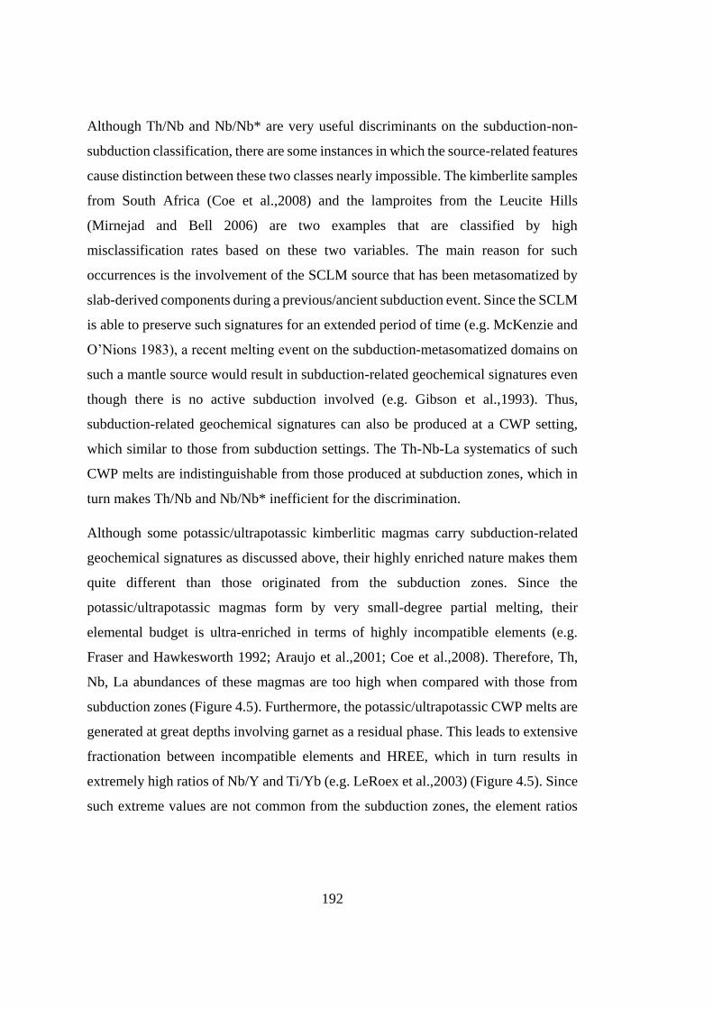
192
Although Th/Nb and Nb/Nb* are very useful discriminants on the subduction-non-
subduction classification, there are some instances in which the source-related features
cause distinction between these two classes nearly impossible. The kimberlite samples
from South Africa (Coe et al.,2008) and the lamproites from the Leucite Hills
(Mirnejad and Bell 2006) are two examples that are classified by high
misclassification rates based on these two variables. The main reason for such
occurrences is the involvement of the SCLM source that has been metasomatized by
slab-derived components during a previous/ancient subduction event. Since the SCLM
is able to preserve such signatures for an extended period of time (e.g. McKenzie and
O’Nions 1983), a recent melting event on the subduction-metasomatized domains on
such a mantle source would result in subduction-related geochemical signatures even
though there is no active subduction involved (e.g. Gibson et al.,1993). Thus,
subduction-related geochemical signatures can also be produced at a CWP setting,
which similar to those from subduction settings. The Th-Nb-La systematics of such
CWP melts are indistinguishable from those produced at subduction zones, which in
turn makes Th/Nb and Nb/Nb* inefficient for the discrimination.
Although some potassic/ultrapotassic kimberlitic magmas carry subduction-related
geochemical signatures as discussed above, their highly enriched nature makes them
quite different than those originated from the subduction zones. Since the
potassic/ultrapotassic magmas form by very small-degree partial melting, their
elemental budget is ultra-enriched in terms of highly incompatible elements (e.g.
Fraser and Hawkesworth 1992; Araujo et al.,2001; Coe et al.,2008). Therefore, Th,
Nb, La abundances of these magmas are too high when compared with those from
subduction zones (Figure 4.5). Furthermore, the potassic/ultrapotassic CWP melts are
generated at great depths involving garnet as a residual phase. This leads to extensive
fractionation between incompatible elements and HREE, which in turn results in
extremely high ratios of Nb/Y and Ti/Yb (e.g. LeRoex et al.,2003) (Figure 4.5). Since
such extreme values are not common from the subduction zones, the element ratios
193
such as Nb/Y and Ti/Yb can be useful discriminators in the cases that Th/Nb and
Nb/Nb* does not work.
Figure 4.5. Comparison of spider-diagrams between samples continental within-plates and subduction-
related settings (normalization coefficients are based on Sun and McDonough, 1995)
It is seen from the above discussion that some lithologies from CWP settings can be
recovered in the process of tectonomagmatic classification using some of their
petrogenetic features, although they fail at the upper classification levels. Another case
in which the classification is difficult comes from BAB settings. As mentioned in
Chapter 2, the BABs are like a hybrid between MORs and arcs.
As a natural consequence of this dual nature, the magmas generated at the BABs
display a compositional spectrum between these two extremes (e.g. Pearce et
al.,1995b; Leat et al.,2004; Pearce et al.,2005). Some BAB magmas show MORB-like
subduction-immobile chemistry with the addition of subduction component (relative
Th-LREE enrichment), known as “BABB-type” chemistry.
194
Some, on the other hand, exhibit geochemical characteristics close to the end-members
(MORB- and OAB-like). Such BAB magmas are derived from identical mantle
sources to either that of MORBs or OABs. The BAB melts produced by
decompression melting of MORB-source mantle with no subduction influx would be
very akin to melts generated at MORs (Figure 4.6).
Thus, such cases pose a great problem in discrimination of subduction samples (in this
case, BAB) from non-subduction ones (MOR). Therefore, the misclassification
problem between some BABs and MORs does not appear to arise from the
inefficiency of the decision tree classification. Instead, some MOR and BAB melts are
indistinguishable in terms of their trace element systematics.
Figure 4.6. Comparison of spider-diagrams between samples from OBAB misclassified as MOR and
samples from MOR (normalization coefficients are based on Sun and McDonough, 1995)
195
4.2.2. Discrimination Within Subduction Settings
4.2.2.1. The First Path for Discrimination Within Subduction Settings
4.2.2.1.1. Discrimination Between Arc and Back-arc-related Settings
For training and test datasets, the first tree correctly classified 556 samples of arcs out
of 562 with a success ratio of 98.93% and 92 samples of back-arcs out of 106 with a
success ratio of 86.79%. This decision tree is much more successful for the
discrimination of arc samples with respect to back-arc samples. However, this may be
a result of a limited number of samples in back-arcs as reliable data for back-arcs in
literature is also limited. The introduction of Y/Yb at the fourth level increased
correctly classified subduction samples by 8 whereas misclassifications in non-
subduction samples also increased by 4. These misclassifications are solved by the
introduction of Zr/Hf at the fifth level.
A very similar pattern is also observed in the second decision tree. The second decision
tree is less successful for the discrimination of back-arc samples with 89 samples out
of 106 with a success ratio of 83.96%; however, there are no differences for the
discrimination of arc samples.
When the structures of decision trees are evaluated, the first decision tree obtains the
highest success ratio at the fifth level for both tectonic settings, whereas the second
decision tree at the fourth level for back-arcs and the fifth level for arcs. In the second
decision tree, introduction of Zr/Y and Y/Yb at fourth level increased correctly
classified subduction samples by 7 but has no positive or negative effect on non-
subduction samples and Nd/Zr and Zr/Hf at fifth level increased correctly classified
non-subduction samples by 1 whereas misclassifications for subduction samples
increased by 1 at this level.

196
Different than the general trend of their success ratio with an increasing level in
depths, both decision trees are more successful in the lower levels at the discrimination
of arc and back-arc-related settings for external datasets. Both decision trees have their
maximum success ratio at the second level in depth for back-arcs with 68 samples out
of 102 (66.67% success ratio).
The first decision tree is the most successful for discrimination of arcs in the second
and third levels with 348 samples out of 364 (95.60% success ratio), whereas the
second decision tree is the most successful in the third level with 354 samples out of
364 (97.25% success ratio).
For the first decision tree, success for the discrimination of back-arcs decreases with
the introduction of TiO2/Y and Nd/TiO2 at the third level, and that of arcs decreases
with the introduction of Y/Yb at the fourth level. However, these decreases are
negligible compared to the decrease in success for the second decision tree at its fourth
level with the introduction of Zr/Y and Y/Yb, which results in an additional 10
misclassifications for back-arcs and 4 misclassifications for arcs.
Both decision trees are more successful for the discrimination of arcs with respect to
that of back-arcs for both training+test datasets and external datasets.
When the contradiction between the success ratios of both decision trees at the
discrimination of training+test datasets and external datasets, it shall be assumed that
deeper decision trees may be more successful at the discrimination of training and test
set but fail more for the discrimination of external datasets, resulting in overfitting.
Therefore, considering the results for training+test sets and external datasets, fourth
and fifth levels shall be preferred considering the geochemical and petrological
properties of rock samples and comparison with article-based discussion.
The first decision tree obtained a very high success ratio for all datasets (more than
90% overall) and became more successful for samples of arc with respect to those of
back-arc-related settings. The success ratio of this decision tree is distributed
197
homogeneously through the articles from different locations, with a few exceptions
for the training and test datasets.
For training and test datasets, 18 articles out of 26 having 411 samples are classified
correctly with 100% success ratio. 8 articles have misclassifications with varying
misclassification ratios. Continental arcs and oceanic arcs quite successful for the
discrimination between arc and back-arc-related settings. Misclassifications for the
first decision tree are only 3 samples of continental arcs out of 181 from 7 articles and
3 samples of oceanic arcs out of 381 from 14 articles. Similarly, with the
discrimination between subduction and non-subduction settings, oceanic back-arcs
have misclassification through all articles. Only one article (Leat, 2004 of South
Sandwich) can be completely classified.
However, the misclassification rates for this classification are relatively lower than the
first set of classifications between subduction and non-subduction. 25
misclassifications through 106 samples of oceanic back-arcs from 5 articles result in
a success ratio of 76.42%. The increasing level of depth for the first decision tree
seems to have no significant positive or negative effect for the misclassifications at
the first level with few exceptions. Todd (2012) of Fiji Tonga and Peate (1997) of
Vanuatu are correctly classified at the second level, and Jolly (2007) of Greater
Antilles Arcs is only misclassified at the fourth level. For other articles, there is no
obvious difference between level 1 and level 5. Therefore, levels 3, 4 and 5 shall be
used for discrimination between arc and back-arc-related settings without having a
significant difference in their success ratios.
The first decision tree is also successfully applicable for the tectono-magmatic
discrimination of external datasets. For external datasets, 15 articles out of 26 having
293 samples are classified correctly with 100% success ratio. 11 articles have
misclassifications with varying misclassification ratios. Continental arcs are
completely classified with 100% success ratio at all levels of this decision tree. This
result indicates that Nb/Nb* ratio is quite effective discriminating feature for these

198
tectonic settings. Oceanic arcs are quite successful for the discrimination between arc
and back-arc-related settings. Misclassification for the second tree is 17 samples of
oceanic arcs out of 223 from 12 articles. Oceanic back-arcs are still problematic and
can be discriminated with relatively lower success ratios in the discrimination between
arc and back-arc-related settings. 40 misclassifications out of 102 samples from 6
articles result in a very low success ratio of 60.78%. Harrison (2003) of East Scotia
and Sinton (2003) of Mantus are completely misclassified. Only Bezos (2009) of Lau
Basin can be correctly classified with 100% success ratio. Ikeda (2003) of Mariana
has 3 misclassifications out of 15 samples with a success ratio of 80%. The other two
articles have misclassifications 50% and 67%, respectively.
The problem for the correct classification of oceanic back-arcs in the discrimination
of arc and back-arc-related settings, as well as between subduction and non-
subduction settings can not be solved in training and test datasets and is also observed
in external datasets. The second decision tree is successfully applicable for the
tectono-magmatic discrimination of training and test datasets, and the results are quite
similar to those obtained from the first decision tree but with better success ratios.
For training and test datasets, 19 articles out of 26 having 508 samples are classified
correctly with 100% success ratio. 7 articles have misclassifications with varying
misclassification ratios. Continental arcs and oceanic arcs quite successful for the
discrimination between arc and back-arc-related settings. Misclassifications for the
first decision tree are only 4 samples of continental arcs out of 181 from 7 articles and
2 samples of oceanic arcs out of 381 from 14 articles. Similarly, with the first decision
tree, oceanic back-arcs have misclassification through all articles. Only one article
(Leat, 2004 of South Sandwich) can be completely classified. The misclassification
rates for the second decision tree are relatively higher with respect to the first decision
tree. 29 misclassifications through 106 samples of oceanic back-arcs from 5 articles
result in a success ratio of 72.64%, with a decrease of 3.78%. The increasing level of
depth for the second decision tree seems to have no significant positive or negative
effect for the misclassifications at the first level with few exceptions. Only Peate

199
(1997) of Vanuatu are correctly classified at the fourth level, and Jolly (2007) of
Greater Antilles Arcs can also be classified at the fourth level. For other articles, there
is no obvious difference between level 1 and level 5. Therefore, levels 3, 4 and 5 shall
be used for discrimination between arc and back-arc-related settings without having a
significant difference in their success ratios.
The second decision tree is also successfully applicable to the tectono-magmatic
discrimination of external datasets. For external datasets, 14 articles out of 26 having
287 samples are classified correctly with 100% success ratio. 12 articles have
misclassifications with varying misclassification ratios. Continental arcs are
completely classified with 100% success ratio at all levels of this decision tree. This
result indicates that Nb/Nb* ratio is quite effective discriminating feature for these
tectonic settings. Oceanic arcs are quite successful for the discrimination between arc
and back-arc-related settings. Misclassification for the second tree is 13 samples of
oceanic arcs out of 223 from 12 articles. Oceanic back-arcs are still problematic and
can be discriminated with relatively lower success ratios in the discrimination between
arc and back-arc-related settings. 44 misclassifications out of 102 samples from 6
articles result in a very low success ratio of 56.86%. Harrison (2003) of East Scotia
and Sinton (2003) of Manus are completely misclassified. Only Bezos (2009) of Lau
Basin can be correctly classified with 100% success ratio. Ikeda (2003) of Mariana
has 4 misclassifications out of 15 samples with a success ratio of 73%. The other two
articles have misclassifications 58% and 73%, respectively. The problem for the
correct classification of oceanic back-arcs in the discrimination of arc and back-arc-
related settings, as well as between subduction and non-subduction settings, can not
be solved in training and test datasets and is also observed in external datasets.
The discrimination between arcs and oceanic back-arcs appears to be resolved with
relatively high classification rates. One of the reasons for this lies behind the spreading
factor of the mature oceanic back-arcs (see Chapter 1 for details), which tend to
200
involve more MORB mantle component with less subduction input (leading to higher
Nb/Nb*).
The arcs, on the other hand, include a strong subduction component in their
petrogenesis (resulting in lower Nb/Nb*). Thus, Nb/Nb* ratio (found lesser in oceanic
back-arcs, but more in arcs) works well as an efficient discriminant for arcs and
oceanic back-arcs, by filtering about 90% arcs at the first level of the decision tree.
Also, Nd/Zr ratio, which can be strongly fractionated based on the contribution from
sediment melt, seem to operate efficiently for the lower levels after Nb/Nb* filter.
In this discrimination, one of the major factors for misclassification of some oceanic
backarcs arises from their significant subduction component. Although spreading
backarcs mainly tap a mantle source somewhat similar to that of MORs, the amount
of subduction component may change among the segments based on factors, including
arc proximity and direction of mantle flow. Thus, the lavas produced in some segments
can possess strong subduction signatures, with high Nb/Nb* ratios. This causes such
backarc lavas to resemble those from arcs, which in turn leads their misclassification.
4.2.2.1.2. Discrimination Within Arc-related Settings
For training and test datasets, the first decision tree correctly classified maximum 370
samples of oceanic arcs out of 381 with a success ratio of 97.11% at its seventh level
and 168 samples of continental arcs out of 181 with a success ratio of 92.82% at its
third level. The introduction of Zr/TiO2, La/Yb and Y/Yb at fourth level drastically
decreases the successful classification rate of the first decision tree for continental arcs
by 48 misclassifications and this negative effect could only be solved with the
introduction of Zr/Sm and La/Nb at sixth level. However, the introduction of the ratios
at the fourth level has a great positive effect at the classification rate of oceanic arcs
with 77 additional correct classifications. Therefore, if a simple decision tree is to be
preferred for the first decision tree, the third level shall be preferred for rocks of
continental origin, and the fourth level shall be preferred for rocks of oceanic origin.
201
However, if this information is limited or not available, the seventh level of the first
decision tree shall be used for both tectonic settings.
The same trend is also observed for the second decision tree. The introduction of
Th/La, Sm/Hf, and Zr/Y at the fourth level has a negative effect on the discrimination
of oceanic arcs with a decrease by 16 and positive effect on the discrimination of
continental arcs with an increase by 44. However, the general trend is an increase in
the success ratio for both tectonic settings with an increase of level in depth for the
second decision tree. This decision tree correctly classified 372 samples of oceanic
arcs out of 381 with a success ratio of 97.64% and 171 samples of continental arcs out
of 181 with a success ratio of 94.48%.
The first decision tree correctly classified maximum 176 samples of continental arcs
out of 223 with a success ratio of 78.93% at the fifth level and 136 samples of oceanic
arcs out of 141 with a success ratio of 96.45% at second and third levels. The
introduction of Zr/TiO2, La/Yb, and Y/Yb at the fourth level drastically decreases the
success ratio for the discrimination of continental arcs with a decrease by 53, and this
negative effect cannot be solved for the deeper levels of the first decision tree.
Therefore, overfitting for the classification of continental arcs can be assumed starting
from the fourth level of the decision tree. Interestingly, the introduction of ratios at the
fourth level increases the success ratio for the discrimination of oceanic arcs with an
increase by 76. However, starting from the fifth level, the success ratio for the
discrimination of oceanic arcs also decreases with an increasing level of depth similar
to that of continental arcs in the first decision tree. When the classification results of
the first decision tree for the external dataset are examined, second and third levels
shall be preferred if the origin of rocks are continental, fourth, and fifth levels shall be
preferred if the origin of rocks are oceanic. Deeper levels are assumed to result in
overfitting, which results in the failure of a decision tree when applied to external
datasets.

202
The second decision tree correctly classified maximum 178 samples of continental
arcs out of 223 with a success ratio of 79.82% at the seventh level and 108 samples of
oceanic arcs out of 141 with a success ratio of 76.60% at sixth level. The success ratio
for the second decision tree increases with an increasing level of depth. Therefore, no
overfitting is observed in the second decision tree. The second decision tree is indeed
successful for the discrimination of oceanic arcs in the second and third levels, but this
success decreases with the introduction of Th/La, Sm/Hf, and Zr/Y at the fourth level
with a decrease by 37. This negative effect is solved with the introduction of La/Y,
Sm/Nd, Nb/Nb*, Sm/Hf and La/Nb at the fifth level. For the discrimination of oceanic
arcs, on the other hand, there is a continuous increase in the success ratio. When the
classification results of the second decision tree for the external dataset are examined,
the seventh level shall be preferred for discrimination of oceanic arcs and continental
arcs.
The first decision tree is much more successful for the discrimination of continental
arcs, and the second decision tree is relatively more successful for the discrimination
of oceanic arcs.
The first decision tree obtained a very high success ratio for all datasets and became
successful for samples of both oceanic arcs and continental arcs. The success ratio of
this decision tree is distributed homogeneously through the articles from different
locations, with few exceptions for the training and test datasets.
For training and test datasets, only 6 articles out of 21 having 63 samples are classified
correctly with 100% success ratio. 15 articles have misclassifications with varying
misclassification ratios. No settings are completely classified with 100% success ratio.
Misclassifications for the first decision tree are 18 samples of continental arcs out of
181 from 7 articles and 19 samples of oceanic arcs out of 381 from 14 articles.
For continental arcs, misclassifications generally tend to increase at the fourth and
fifth levels with the introduction of Zr/TiO2, La/Yb and Y/Yb at the fourth level, Y/Yb,
Sm/Hf and Zr/Hf at fifth level. Portnyogin (2015) of Kamchatka and Simon (2014) of
203
Kamchatka can be completely classified with a success ratio of 100%. Gertisser (2000)
of Aeolian, on the other hand, can be correctly classified at the sixth level with a
success ratio of 100% but with the introduction of Sm/Hf and Zr/Hf at seventh level,
4 misclassifications are observed with a misclassification rate of 80%. Other than this
article, misclassification rates for the sixth and seventh levels for all articles of
continental arcs are low within a range of 8-20%.
For oceanic arcs, misclassifications are highly dominated in first levels with less and
homogeneous distribution through higher levels. Bedard (1999) of Canada,
Hochstaedter (2001) of Izu Bonin, Pearce (2005) of Mariana, Schuth (2004) of
Solomon Islands and Yogodzinski (2015) of Western Auletian can be completely
classified with a success ratio of 100%. Hickey and Vargas (2013) of Daito can be
correctly classified at fifth level but 2 and 1 misclassifications with a success ratio of
25% and 13%, with respectively in sixth and seventh levels with the introduction of
Sm/Hf, Zr/Nb, La/Y, Th/La and Nb/Y at sixth level and Sm/Y, Nb/Nb* and Zr/Hf at
seventh level.
Other than this article, misclassification rates for the sixth and seventh levels for all
articles of oceanic arcs are low within a range of 3-27%. The first decision tree is
successful for the discrimination of oceanic and continental arcs at its sixth and
seventh levels; therefore, these levels shall be preferred.
The first decision tree is more successfully for the tectono-magmatic discrimination
of external datasets.
For external datasets, 16 articles out of 26 having 306 samples are classified correctly
with 100% success ratio. 10 articles have misclassifications with varying
misclassification ratios. For external datasets, the success ratio for the classification
of continental arcs decreases much more with respect to that of oceanic arcs, especially
with the increasing level of depth. Bryant (2006) of Andes, De Astis (1997) of
Aeolian, Santo (2004) of Aeolian and Zelenski (2018) of Kamchatka can be
completely classified with a success ratio of 100% whereas Bailey (2009) of Santorini,
204
Calanchi (2002) of Aeolian, De Astis (2000) of Aeolian and Ianelli (2017) of North
Patagonian Andes can be classified with 1-2 misclassification errors in the second and
third levels. However, for deeper levels of the first decision tree, success ratio
drastically falls, and an overfitting is clearly observed for the discrimination of
continental arcs for the levels above fourth level, with the introduction of Zr/TiO2,
La/Yb and Y/Yb at fourth level, Y/Yb, Sm/Hf and Zr/Hf at fifth level, Nb/Nb*, Zr/Sm
and La/Nb at sixth level and Nb/Y, Th/Y, Sm/Hf and Zr/Hf at seventh level, resulting
64 more misclassifications in continental arcs. However, this situation changes in the
opposite direction for the classification of oceanic arcs within the discrimination
between continental and oceanic arcs. Most of the articles can be classified more
accurately with the increasing level of depth with an increase of correctly classified
samples by 51. Finney (2008) of Okmok, König (2008, 2010) of various subduction
zones, Stellin (2002) of Shishaldin, Tamura (2011) of Mariana, Bezos (2009) of Lau
Basin, Harrison (2003) of East Scotia, Ikeda (2016) of Mariana, Ishizuka (2009) of
Izu Bonin, Mortimer (2007) of South Fiji and Sinton (2003) of Manus are all articles,
correctly classified with a success ratio of 100%. The misclassification for oceanic
arcs decreases down to 66 out of 325, with a success ratio of 79.69%. Therefore, the
application of the first decision tree to the discrimination between oceanic arcs and
continental arcs are complicated and may require a cross-check with the application
of another decision tree developed for the discrimination between oceanic and
continental settings. If the sample is known or thought to be of oceanic in origin, then
the sixth or seventh levels of the first decision tree shall be preferred more
conveniently or the second or third levels shall be preferred if it is of continental in
origin. The second decision tree is successfully applicable for the tectono-magmatic
discrimination of training and test datasets, and the results are quite similar to those
obtained from the first decision tree but with better success ratios. For training and
test datasets, 7 articles out of 21 having 121 samples are classified correctly with 100%
success ratio. 14 articles have misclassifications with varying misclassification ratios.
However, misclassification ratios through articles are more homogeneous and smaller
with respect to those in the first decision tree, ranging between 7-20% with quite a few
205
exceptions. For continental arcs, Portnyogin (2015) of Kamchatka, Metrich (2001) of
Aeolian, and Simon (2014) of Kamchatka can be correctly classified at either sixth or
seventh levels.
Total misclassifications for continental arcs for discrimination between continental
and oceanic arcs are 10 samples out of 181 from 7 articles. Only Gertisser (2000) of
Aeolian has a misclassification rate of 40% with 2 misclassifications. Other articles
have less than 10% misclassification rates with 1-3 misclassifications. For oceanic
arcs, Hochstaedter (2001) of Izu Bonin, Hickey and Vargas (2013) of Daito, Pearce
(1995) of South Sandwich, Pearce (2005) of Mariana, Peate (1997) of Vanuatu, Schuth
(2004) of Solomon Islands and Yogodzinski (2015) of Western Auletian are correctly
classified with a success ratio of 100% in either sixth or seventh level of the second
decision tree. Similarly, to continental arcs, total misclassifications for oceanic arcs
are also more homogeneously distributed through articles with fewer misclassification
ratios, ranging between 3% and 25% with misclassifications ranging between 1-3 for
each article with one exception (10 misclassifications out of 45).
The second decision tree is also successfully applicable for the tectono-magmatic
discrimination of external datasets. For external datasets, only 4 articles out of 20
having 14 samples are classified correctly with 100% success ratio. 16 articles have
misclassifications with varying misclassification ratios.
For continental arcs, Bryant (2006) of Andes and Zelenski (2018) of Kamchatka are
correctly classified with a success ratio of 100%. Only Santo (2004) of Aeolian has a
misclassification rate of 39% with 12 misclassifications out of 31 samples. However,
other articles of continental arcs have limited misclassifications with ratios ranging
between a narrow range of 17-25% with misclassifications ranging between 2-5%.
For oceanic arcs, Finney (2008) of Okmok and Stellin (2002) of Shishaldin can be
correctly classified with a success ratio of 100%. Two articles of oceanic arcs, Jolly
(2008) of Greater Antilles Arc and Straub (2010) of Izu Bonin have misclassifications
greater than 10. Other articles have misclassifications in a range of 1-3 with

206
misclassification ratios of 9-33%. The second decision tree is much more successful
at greater depths for the discrimination of both oceanic arcs and continental arcs.
For oceanic arcs, only for the fourth level, the success ratio decreases drastically with
the introduction of Th/La, Sm/Hf and Zr/Y by a decrease of 37. However, these
misclassifications are solved with the introduction of La/Y, Sm/Nd, Nb/Nb*, Sm/Hf
and La/Nb at the fifth level. The success ratio for discrimination of continental arcs
continually increases with the increasing levels of decision tree and reaches its
maximum at the sixth level with 108 correct classifications and to 107 at the seventh
level. When the success ratio of the second decision tree for discrimination of oceanic
arcs and continental arcs are evaluated and compared to the first decision tree, second
decision tree shall be accepted to be more successful, especially for the highest levels
(sixth and seventh) and shall be preferred for discrimination of both oceanic arcs and
continental arcs without requiring any cross-check with other discriminations. The
sixth and seventh level of the second decision tree is notably much more successful
with respect to the first decision tree and to lowest levels of itself with an increase of
correct classifications by 53 (as double as from 54 to 107).
The discrimination between the oceanic and continental arcs is not straightforward,
like that between arcs and backarcs. In this case, since both classes (oceanic arcs and
continental arcs) include a significant amount of subduction component in their
petrogenesis, it is not surprising that the ratios Th/Nb and Nb/Nb* do not work at the
uppermost level for the discrimination between oceanic and continental arcs.
However, the ratios like Zr/TiO2 and Zr/Sm are able to make a first-order separation,
mainly for the oceanic arcs.
Since the oceanic arcs generally involve highly depleted source regions, they tend to
have lower ratios of Zr/Ti and Zr/Sm when compared with continental arcs. This
filtering appears to work at the upper levels, by constraining a large number of oceanic
arcs. Another useful feature seems to be Sm/Y. High Sm/Y coupled with high Zr/Sm
ratios are more common in continental arcs than oceanic arcs. Indeed, the Sm/Y

207
achieves to filter oceanic and continental arcs for a reasonable success rate at the upper
levels of the decision tree.
4.2.2.2. The Second Path for Discrimination Within Subduction Settings
4.2.2.2.1. Discrimination Between Oceanic and Continental Settings
For training and test datasets, the first decision tree correctly classified a maximum of
467 samples of oceanic setting out of 487 with a success ratio of 95.89% at the sixth
level and 163 samples of continental setting out of 181 with a success ratio of 90.06%
at sixth level. The success ratio of classification of the first decision tree continuously
increasing with increasing level of depth, therefore, without any doubt for training and
test datasets, the sixth level of the first decision tree shall be preferred for the
discrimination of oceanic and continental settings.
The second decision tree shows the same trend with the first decision tree, with a
continuous increase in the success of classification for both oceanic and continental
settings. The second decision tree correctly classified a maximum of 467 samples of
oceanic setting out of 487 with a success ratio of 95.89% at the sixth level and 151
samples of continental setting out of 181 with a success ratio of 83.43% at sixth level.
When classification results for training and test datasets are examined, both decision
trees have the same success for discrimination of oceanic settings but the first decision
tree is much more successful for the discrimination of continental settings. Therefore,
for a general application, the sixth level of the first decision tree shall be preferred.
This is an indication for the positive effect of TiO2-related ratios.
The first decision tree correctly classified 274 samples of oceanic settings out of 325
with a success ratio of 84.31% at second and third levels and 113 samples of
continental settings out of 141 with a success ratio of 80.15% at second and third
levels. The success ratio of the decision tree at higher levels gradually decreases as an
208
indicator of overfitting. The introduction of Zr/Y and Nd/TiO2 at fourth level, Y/Yb,
TiO2/Y, Nb/Nb*, Zr/Hf and Sm/Hf at fifth level and La/Yb, Y/Yb, Sm/Hf and
Nd/TiO2 at sixth level affects negatively the classification ratio of oceanic settings.
Classification of continental settings, on the other hand, is negatively affected only by
the introduction of Zr/Y and Nd/TiO2 at the fourth level. Therefore, the second and
third levels of the first decision tree shall be preferred when classification results of
external datasets are considered.
The second decision tree correctly classified 302 samples of oceanic settings out of
325 with a success ratio of 92.92% at the sixth level and 100 samples of continental
settings out of 141 with a success ratio of 70.92% at second and third levels. As
previously mentioned, the second decision tree fails as a result of overfitting for the
discrimination of continental settings. When the classification of external datasets is
considered, the sixth level of the second decision tree shall be preferred for the
discrimination of oceanic settings if the origin of rock is known to be oceanic. For
both decision tree, success ratio decreases drastically for discrimination of continental
settings, with a decrease by 29 for the first decision tree with the introduction of Zr/Y
and Nd/TiO2 at fourth level and by 28 for the second decision tree Zr/Y and Sm/Y at
the fourth level.
The first decision tree obtained a very high success ratio for all datasets and became
more successful for samples of oceanic settings with respect to those of continental
settings. The success ratio of this decision tree is distributed homogeneously through
the articles from different locations for the training and test datasets.
For training and test datasets, 11 articles out of 26 having 124 samples are classified
correctly with 100% success ratio. 15 articles have misclassifications with varying
misclassification ratios. The first decision tree is quite successful for the classification
of oceanic back-arcs for the discrimination between oceanic and continental settings.
Only one article, Pearce (2005) of Mariana has 1 misclassification for each and 2 in
total out of 70 samples. Other articles of oceanic back-arcs can be correctly classified

209
with 100% success ratio. The first stage of the second path, which first discriminates
between oceanic and continental settings, is more successful in discrimination of
oceanic back-arcs rather than discriminating between arc and back-arc-related
settings.
For continental arcs, Metrich (2001) of Aeolian, Portnyogin (2015) of Kamchatka can
be correctly classified in fifth and sixth levels of the first decision tree. The other
articles of continental arcs have limited misclassifications with ratios ranging between
4% and 14%. The only exception is Gertisser (2000) of Aeolian, which completely
fails in the first decision tree at all levels.
The fifth and sixth levels of the first decision tree are more successful with respect to
lower levels. For instance, the misclassifications in Hickey Vargas (2016) of Chile
decreases from 14 (41%) to 3 (9%) with the introduction of Y/Yb, TiO2/Y, Nb/Nb*,
Zr/Hf and Sm/Hf at fifth level and La/Yb, Y/Yb, Sm/Hf and Nd/TiO2 at sixth level.
For oceanic arcs, Bedard (1999) of Canada, Hochstaedter (2001) of Izu Bonin, Pearce
(2005) of South Sandwich, Pearce (2005) of Mariana, Schuth (2004) of Solomon
Islands, Tollstrup (2010) of Izu Bonin and Yogodzinski (2015) of Western Auleatian
can be correctly classified with a success ratio of 100% for the fifth and sixth levels
of the first decision tree. Total misclassifications for oceanic arcs in the discrimination
between oceanic and continental settings are 18 out of 381 from 14 articles with
misclassifications ranging between 2 and 3, with ratios ranging between 3% and 13%.
When success ratio of the first decision tree for discrimination between oceanic and
continental settings, especially higher levels are much more successful, and their
success increases with the introduction of Y/Yb, TiO2/Y, Nb/Nb*, Zr/Hf and Sm/Hf
at fifth level and La/Yb, Y/Yb, Sm/Hf and Nd/TiO2 at sixth level.
The first decision tree is also successfully applicable for the tectono-magmatic
discrimination of external datasets. For external datasets, only 5 articles out of 26
having 35 samples are classified correctly with 100% success ratio. 21 articles have
misclassifications with varying misclassification ratios. For continental arcs, Zelenski

210
(2018) of Kamchatka can be correctly classified with a success ratio of 100% at all
levels. However, Bryant (2006) of Andes and Ianelli (2017) of North Patagonian,
Andes can be correctly classified at lower levels (second and third) in spite of having
misclassifications in higher levels, especially with the introduction of Zr/Y and
Nd/TiO2 at fourth level, Y/Yb, TiO2/Y, Nb/Nb*, Zr/Hf and Sm/Hf at fifth level. For
oceanic arcs, Finney (2008) of Okmok, Stellin (2002) of Shishaldin and Tamura
(2011) of Mariana can be correctly classified with a success ratio of 100% at all levels
of the first decision tree. Total misclassifications for oceanic arcs are 59 out of 223
from 12 articles, and misclassifications are homogeneously distributed to all articles
with quite a few exceptions. Only Pearce (1999) of Western Pacific fails in the
discrimination with a misclassification ratio of 80%. For König (2008, 2010) from
various subduction zones, the first decision tree is successful for lower levels but
misclassifications are observed in higher levels with the introduction of Y/Yb, TiO2/Y,
Nb/Nb*, Zr/Hf and Sm/Hf at fifth level and La/Yb, Y/Yb, Sm/Hf and Nd/TiO2 at sixth
level. For oceanic back-arcs, Harrison (2003) of East Scotia can be correctly classified
with a success ratio of 100%. Bezos (2009) of Lau Basin, Ikeda (2016) of Mariana
and Sinton (2003) of Manus can be classified in the second or third levels of the first
decision tree, but misclassifications are observed at higher levels.
The second decision tree is successfully applicable for the tectono-magmatic
discrimination of training and test datasets, and the results are quite similar to those
obtained from the first decision tree but with relatively lower success ratios. For
training and test datasets, 10 articles out of 26 having 148 samples are classified
correctly with 100% success ratio. 16 articles have misclassifications with varying
misclassification ratios. The second decision tree is quite successful for the
discrimination of oceanic back-arcs. For oceanic back-arcs, Beier (2015) of Manus
Basin and Leat (2004) of South Sandwich Pearce (1995) of Lau and Pearce (2005) of
Mariana can be correctly classified within the discrimination between oceanic and
continental settings.
211
For continental arcs, Gertisser (2000) of Aeolian fails at classification with a
misclassification ratio of 100% out of 5 samples. Mullen (2017) of Cascade Arc also
has problems with 50% misclassification ratio. Portnyogin (2015) of Kamchatka can
be correctly classified with a success ratio of 100%. Other articles have quite a few
misclassifications ranging between 1 and 3. For oceanic arcs, Bedard (1999) of
Canada, Hochstaedter (2001) of Izu Bonin, Schuth (2004) of Solomon Islands, Pearce
(1995) of Lau and Pearce (2005) of Mariana can be correctly classified at fifth and
sixth levels. There are quite a few misclassifications in discrimination of oceanic arcs
with misclassification ratios ranging between 2% and 13%. With a few exceptions,
fifth and sixth levels of the second tree shall be preferred for discrimination between
oceanic and continental settings as success ratio increases with increasing level of the
decision tree, by 16 samples for oceanic settings and by 51 for continental settings.
Starting from the fourth level, the addition of each level has a positive impact on the
classification of both oceanic and continental settings.
The second decision tree is also successfully applicable for the tectono-magmatic
discrimination of oceanic settings in external datasets; however, the success ratio for
discrimination of continental settings gradually decreases with increasing level of
depth in the second decision tree.
For external datasets, 9 articles out of 26 having 104 samples are classified correctly
with 100% success ratio. 17 articles have misclassifications with varying
misclassification ratios. The second decision tree is also successful for the correct
classification of oceanic back-arcs in external datasets. Only 9 misclassifications for
oceanic back-arcs are observed out of 102 samples from 6 articles. Bezos (2009) of
Lau Basin, Harrison (2003) of East Scotia, and Sinton (2003) of Manus can be
correctly classified with a success ratio of 100%. Sixth level of this decision tree is
especially quite successful with the positive impacts of the addition of higher levels
and introduction of Zr/Y and Sm/Y at fourth level, Y/Yb, Nb/Nb*, Zr/Hf and Sm/Hf
at fifth level and La/Yb, Zr/Y, Zr/Hf and La/Nb at sixth level. For oceanic arcs, Finney
(2008) of Okmok, König (2008 and 2010) of various subduction zones, Stellin (2002)
212
of Shishaldin, Tamura (2011) of Mariana and Woodhead (2001) of different locations
can be correctly classified with a success ratio of 100%. Jolly (2008) of Greater
Antilles Arc has 15 misclassifications that form the majority of misclassifications in
oceanic arcs.
These misclassifications cannot be solved at any stage of the second decision tree,
however, they increase at the fourth level with the introduction of Zr/Y and Sm/Y and
decrease at the fifth level with the introduction of Y/Yb, Nb/Nb*, Zr/Hf and Sm/Hf.
Other articles have few misclassifications with ratios ranging between 9% and 20%.
Discrimination of continental arcs in external datasets is problematic as
misclassifications increase in nearly all articles. No articles cannot be correctly
classified with all of its samples. Calanchi (2002) of Aeolian fails for discrimination
with a misclassification ratio of 100%. Other major failures are Bailey (2009) of
Santorini and Santo (2004) of Aeolian with misclassification ratio greater than 50%.
Other articles have, on the other hand, misclassifications less than 10. The second
decision tree is more successful at the discrimination of oceanic settings with respect
to continental settings when the application to external datasets is evaluated.
Overfitting can be possible for continental settings, especially for continental arcs.
However, as the best choice, the fifth level of the second decision tree shall be
preferred.
Among two decision trees, the first decision tree is more successful for discrimination
of continental settings, and the second decision tree is more successful for
discrimination of oceanic settings. In both decision trees, success ratios decrease with
increasing levels of depth for continental settings of external datasets. Therefore,
considering the classification results of both training-test and external datasets, the
fifth and sixth levels of the first decision tree along with the fifth level of the second
decision tree shall be preferred, and a cross-check shall be applied.
For the classification of continental and oceanic settings, the strong subduction
fingerprint Nb/Nb* is not preferred at the top of the classification. This case is very
213
similar to that between continental and oceanic arcs since the subduction component
is very strong within the two classes, namely continental arcs, and oceanic arcs and
back-arcs. This time Zr/Y ratio appears to do a good job at the first level of
discrimination. In the oceanic arcs and back-arcs, the source region is generally
depleted (characterized by N-MORB source mantle or even depleted) than that of
continental arcs. The exceptions are few and include some oceanic arcs and back-arcs
that has produced enriched lavas. The continental arcs, on the other hand, may involve
relatively a more enriched mantle source with the involvement of continental
lithospheric mantle, lower-degrees of partial melting and crustal contamination. Thus,
continental arcs can be expected to have higher Zr/Y ratios, in general. This feature
really seems to be efficient, allocating a large number of oceanic arcs and back-arcs
towards the low Zr/Y side.
4.2.2.2.2. Discrimination Within Oceanic Settings
For training and test datasets, the first decision tree correctly classified a maximum of
378 samples of oceanic arcs out of 381 with a success ratio of 99.21% at the second
level, and 98 samples of oceanic back-arc basins out of 106 with a success ratio of
92.45% at sixth level.
The second tree correctly classified maximum 378 samples of oceanic arcs out of 381
with a success ratio of 99.21% at the second level and 99 samples of oceanic back-arc
basins out of 106 with a success ratio of 93.4% at sixth level.
When the classification results of two decision trees are examined for training and test
datasets, when a simple structure is to be preferred, second level of both decision trees
is a good discriminator for oceanic arcs but for a general purpose, sixth level of
decision trees shall be preferred for discrimination between oceanic arcs and oceanic
back-arcs. If the origin of rock is considered to be of a back-arc, then the second levels
of both decision trees shall be applied.
214
Both decision trees much more successfully discriminate oceanic arcs when compared
to oceanic back-arcs for training and test datasets.
The first decision tree correctly classified maximum 219 samples of oceanic arcs out
of 223 with a success ratio of 98.21% at second and third levels and 81 samples of
oceanic back-arc basins out of 102 with a success ratio of 79.41% sixth levels. The
second decision tree obtained the same maximum success ratios at the same levels
with the first decision trees.
For both decision trees, the classification rate increases with the increasing level of
depth for oceanic back-arcs until the fourth level, but deeper levels have no significant
positive or negative effect on the success ratio.
The greater levels in the first decision tree show fluctuations. The success ratio for
discrimination of oceanic arcs decreases with the introduction of Nb/Nb*, Nd/Zr and
TiO2/Yb at the fourth level and Y/Yb and Nb/Yb at sixth level but increases with the
introduction of Nb/Nb* and Zr/Hf at fifth level.
However, the success ratio for the discrimination of oceanic arcs at the greater levels
in the second decision tree continuously decreases with the introduction of Nd/Zr and
La/Sm at the fourth level, Nb/Nb* and Sm/Y at fifth level and Y/Yb at sixth level.
This is an indication of overfitting that much deeper decision trees ignoring TiO2-
related ratios would be expected to fail more at external datasets.
When their success ratios for discrimination of external datasets are examined, if the
origin of rock is thought to be arc-related then second and third levels of the first
decision tree, otherwise, fifth and sixth levels of the first decision tree shall be
preferred. For the second decision tree, the fourth level shall be preferred for
discrimination between oceanic arcs and oceanic back-arcs.
The first decision tree obtained a very high success ratio, especially for oceanic arcs.
The discrimination of oceanic back-arcs is, on the other hand, is a little problematic
215
with a lower success ratio. The success ratio of this decision tree is distributed
homogeneously through the articles from different locations, with a few exceptions
for the training and test datasets.
For training and test datasets, 12 articles out of 19 having 347 samples are classified
correctly with 100% success ratio. 7 articles have misclassifications with varying
misclassification ratios. For oceanic arcs, Hickey and Vargas (2013) of Daito, Jolly
(2007 and 2008) of Greater Antilles Arc, Pearce (1995) of South Sandwich, Pearce
(2005) of Mariana, Rojas and Agramonte (2017) of Lesser Antilles, Schuth (2004) of
Solomon Islands, Singer (2007) of Auletian, Tollstrup (2010) of Izu Bonin and
Yogodzinski (2015) of Western Auletian can be correctly classified with a success
ratio of 100% at sixth level. Hochstaedter (2001) of Izu Bonin and Peate (1997) of
Vanuatu can be correctly classified at third or fifth levels, but with the introduction of
Nd/Zr and TiO2/Yb at fourth level and Y/Yb and Nb/Yb at the sixth level, their
discrimination ratios decrease with misclassifications. For oceanic back-arcs, 20
misclassifications out of 106 samples from 5 articles are observed in the
discrimination between oceanic arcs and oceanic back-arcs. Leat (2004) of Sandwich
and Pearce (1995) of Lau can be correctly classified with a success ratio of 100%.
When the classification results for the discrimination of oceanic arcs and oceanic back
arcs are evaluated for the first decision tree, fifth and sixth levels shall be preferred.
The first decision tree is also successfully applicable for the tectono-magmatic
discrimination of external datasets.
For external datasets, 8 articles out of 18 having 155 samples are classified correctly
with 100% success ratio. 10 articles have misclassifications with varying
misclassification ratios. For oceanic back-arcs, Bezos (2009) of Lau Basin and
Harrison (2003) of East Scotia can be correctly classified with a success ratio of 100%.
Sinton (2003) of Manus, on the other hand, fails completely for this discrimination.
The other three articles have misclassifications ranging between 4 and 6 and ratios
between 20% and 33%. For oceanic arcs, Finney (2008) of Okmok, Jolly (2008) of
216
Greater Antilles Arc, König (2010) of various subduction zones, Leslie (2009) of Fiji
Arc and Stellin (2002) of Shishaldin can be correctly classified with a success ratio of
100%. Other articles have misclassifications ranging between 1 and 5 with a broader
range misclassification ratio as 4-40%. Pearce (1999) of Western Pacific can be
correctly classified at the third level but misclassifications are observed in higher
levels of depth. The first decision tree is more successful, especially for the
discrimination of oceanic back-arcs at higher levels with the introduction of Nd/Zr
and TiO2/Yb at the fourth level, Nb/Nb* and Zr/Hf at fifth level and Y/Yb and Nb/Yb
at sixth level. Therefore, when the classification results for discrimination between
oceanic arcs and oceanic back-arcs are evaluated, fifth and sixth levels of the first
decision tree shall be preferred for the discrimination between oceanic arc and oceanic
back-arcs.
The second decision tree is successfully applicable for the tectono-magmatic
discrimination of training and test datasets, and the results are quite similar to those
obtained from the first decision tree but with better success ratios.
For training and test datasets, 10 articles out of 19 having 212 samples are classified
correctly with 100% success ratio. 9 articles have misclassifications with varying
misclassification ratios. For oceanic arcs, Hickey and Vargas (2013) of Daito, Pearce
(1995) of South Sandwich, Pearce (2005) of Mariana, Rojas and Agramonte (2017)
of Lesser Antilles, Schuth (2004) of Solomon Islands, Singer (2007) of Auletian,
Tollstrup (2010) of Izu Bonin and Yogodzinski (2015) of Western Auletian can be
correctly classified with a success ratio of 100%. Total misclassifications for oceanic
arcs in discrimination between oceanic arcs and oceanic back arcs are 12 out of 381
from 14 articles with a range of 1 to 3 for each article.
The second decision tree is quite successful at oceanic arcs. However, Hochstaedter
(2001) of Izu Bonin, Jolly (2007 and 2008) of Greater Antilles Arc and Peate (1997)
of Vanuatu can be correctly classified at second and third levels; however,
misclassifications are observed in higher levels with introduction of Nd/Zr and La/Sm

217
at fourth level, Nb/Nb* and Sm/Y at fifth level and Y/Yb at sixth level. For oceanic
back-arcs, Leat (2004) of Sandwich and Pearce (1995) of Lau can be correctly
classified with a success ratio of 100% at the sixth level. Other articles have
misclassifications decreasing with increasing level of depth and finally have 19
misclassifications out of 106 samples from 5 articles.
The second decision tree is also successfully applicable for the tectono-magmatic
discrimination of external datasets.
For external datasets, 7 articles out of 26 having 139 samples are classified correctly
with 100% success ratio. 19 articles have misclassifications with varying
misclassification ratios. For oceanic arcs, Finney (2008) of Okmok, Jolly (2008) of
Greater Antilles Arc, König (2010) of various subduction zones, Leslie (2009) of Fiji
Arc and Stellin (2002) of Shishaldin can be correctly classified with a success ratio of
100% at all levels of the second decision tree. Pearce (1999) of Western Pacific,
Tamura (2011) of Mariana and Wharton (1994) of Viti Levu can be classified at
second and third levels whereas misclassifications are observed with the introduction
of Nd/Zr and La/Sm at fourth level, Nb/Nb* and Sm/Y at fifth level and Y/Yb at sixth
level. Ikeda (2016) of Mariana, Ishizuka (2009) of Izu Bonin, Mortimer (2007) of
South Fiji and Sinton (2003) of Manus can be classified with misclassifications
decreasing with increasing levels of depth.
When the classification results of the second decision tree for both training-test and
external datasets are evaluated, fourth, fifth, and sixth levels of both decision trees
shall be preferred with an acceptable amount of misclassifications, especially in
problematic locations with geochemical, petrological complexities.
The Th/Nb ratio, which appears as the major discriminator, is a very sensitive
subduction indicator. The classification this time is very similar to that for arcs and
oceanic-back-arcs, so the same ideas are valid here. The arcs have a stronger
subduction component due to the fluxing of slab-derived fluids/melts into the mantle
218
wedge (e.g. Pearce et al.,2005). This process, however, is weaker in the oceanic back-
arcs with the more contribution from MOR-type mantle, but with less subduction input
(e.g. Leat et al.,2004). Indeed, this idea, so the sensitivity of Th/Nb based on the slab-
derived influx, is proven by the high classification rates with over 90% arcs being
allocated towards the higher Th/Nb ratios. Although it is not effective as Th/Nb, Zr/Hf
appears to be useful as separating half of the arcs with very high efficiency, based on
the depleted character of the arcs with low Zr/Hf ratios.
4.2.3. Discrimination Within Non-Subduction Settings
4.2.3.1. Discrimination Between Group 1 (Mid-Oceanic Ridge and Oceanic
Plateau) and Group 2 (Oceanic Island and Continental Within-plate) Settings
For training and test datasets, the first decision tree correctly classified 812 samples
of group 2 (oceanic islands and continental within-plates) out of 854 with a success
ratio of 95.08% and 1,082 samples of group 1 (mid-oceanic ridge and oceanic
plateaus) out of 1,120 with a success ratio of 96.61%. This decision tree is quite
successful for discrimination of both group 1 and group 2 for training and test datasets.
Discrimination of group 1 is nearly stable to all levels of the first decision tree with
small fluctuations. Misclassification of group 1 increase by 34 with the Th/Nb and
Y/Yb at the third level, but, decreases stepwise at higher levels with introduction of
Zr/ TiO2, La/Nb, Nb/Nb* and La/Sm at fourth level, La/Nb, Nd/Zr and Nb/Yb at fifth
level, TiO2/Y, Nb/Nb* and Zr/Hf and Th/La at seventh level. Th/Nb at the sixth level
has no positive or negative effect on the classification rate of group 1. The first
decision tree becomes much more successful for the discrimination of group 2 with an
increasing level of depth and reaches its maximum 812 correct classifications at the
seventh level with an increase by 49 following the introduction of Zr/Hf and Th/La at
the seventh level. This may indicate that these two ratios seem to be a good indicator
for the problematic samples of group 2, which can not be correctly classified at lower
levels of depth.

219
The second decision tree has a very similar pattern at its increasing levels of depth
when compared to the first decision tree. For training and test datasets, the second
decision tree correctly classified 814 samples of group 2 (oceanic islands and
continental within-plates) out of 854 with a success ratio of 95.32% and 1,082 samples
of group 1 (mid-oceanic ridge and oceanic plateaus) out of 1,120 with a success ratio
of 96.61%. The second decision tree is also quite successful for the discrimination of
both group 1 and group 2 for this discrimination for training and test datasets.
Discrimination of group 1 is nearly stable to all levels of the first decision tree with
small fluctuations. Misclassifications of group 1 increase by 34 with the Th/Nb and
Y/Yb at third level, but, decreases again stepwise at higher level with introduction of
Zr/TiO2, Th/La, La/Nb, Nb/Nb* and La/Sm at fourth level, Sm/Hf, Nd/Zr and Nb/Yb
at fifth level, La/Nb, Nb/Nb* and La/Nb, Nb/Nb* and Th/Nb at sixth level and Nb/Y,
Zr/Hf and Th/La at seventh level have no positive or negative effects on the
classification rate of group 1. The second decision tree also becomes much more
successful for the discrimination of group 2 with increasing level of depth and reaches
to its maximum 814 correct classifications at the seventh level with an increase by 51
following the introduction of Nb/Y, Zr/Hf, and Th/La at the seventh level. This may
indicate that these two ratios seem to be a good indicator for the problematic samples
of group 2, which can not be correctly classified at lower levels of depth.
When the classification rates of two decision trees for training and test datasets are
evaluated and compared to each other, and through different levels of depth, the
seventh levels of both decision trees shall be preferred with only difference of element
ratios. Therefore, the availability of elements in the dataset shall also be a factor to
choose the decision tree or a cross-check shall be done in order to compare their
results.
For external datasets, the first decision tree correctly classified 489 samples of group
2 out of 539 with a success ratio of 90.72% and 1,432 samples of group 1 out of 1467
with a success ratio of 97.61%. For discrimination of group 2 (oceanic islands and
220
continental within-plates), the success ratio of classification increases with increasing
level of depth in the first decision tree and reaches its maximum at the seventh level.
The discrimination of group 1 (mid-oceanic ridges and oceanic plateaus), on the other
hand, has its maximum success ratio of classification at the second level, but the
success ratio drastically decreases at the third level by 174 with the introduction of
Th/Nb and Y/Yb. For higher levels, success ratio increases with increasing level of
depth of the first decision tree but can not reach to the ratio at the second ratio (82
correct classifications less than that of the second level with a success ratio difference
of 3.34%). The introduction of Th/Nb at the sixth level has no positive or negative
effect on the classification rates.
When the classification rates of the first decision tree in the discrimination between
group 1 and group 2 are evaluated, the seventh level of this decision tree shall be
preferred ignoring the success ratio difference for the discrimination of group 1. The
decision tree proves itself to be applicable to external datasets without any serious
classification problems.
The second decision tree correctly classified 489 samples of group 2 out of 539 with
a success ratio of 90.72% and 1,432 samples of group 1 out of 1467 with a success
ratio of 97.61%. The maximum success ratios of two decision trees for discrimination
of both groups are exactly the same. There are also no differences at all for the
classifications of group 2 at each level but slight differences are observed at the
classification of group 1. The success ratio of the second decision tree for group 1 at
the seventh level is 1,356 with an increase of 6 with respect to the first decision tree.
The introduction of Th/La, La/Nb, Nb/Nb* and La/Sm at fourth level, Sm/Hf, Nd/Zr
and Nb/Yb at fifth level, La/Nb, Nb/Nb* and Th/Nb at sixth level, on the other hand,
is more effective and successful in the discrimination of group 1. This may indicate
that ratios of Th with La and Nb may be more effective with respect to that with Nb
only for the discrimination of mid-oceanic ridges and oceanic plateaus in this
discrimination.
221
When the classification rates of the second decision tree in the discrimination between
group 1 and group 2 are evaluated and compared with the first decision tree, the
seventh level of both decision trees shall be preferred ignoring the success ratio
difference for the discrimination of group 1. The decision trees are both successfully
applicable to external datasets without any serious classification problems.
The first decision tree obtained a very high success ratio for all datasets and became
successful for samples of both group 1 and group 2 of non-subduction settings. The
success ratio of this decision tree is distributed homogeneously through the articles
from different locations, with few exceptions for the training and test datasets.
For training and test datasets, only 23 articles out of 37 having 782 samples are
classified correctly with 100% success ratio. 14 articles have misclassifications with
varying misclassification ratios. No settings are entirely classified with 100% success
ratio. The first decision tree is quite successful for the classification of continental
within-plates. Only 4 articles out of 12 have misclassifications: Hanghoj (2003) of
East Greenland, Larsen (2003) of West Greenland, Peate (2003) of East Greenland,
and Rooney (2012) of Afar Plume have misclassifications of 4, 5, 1 and 1, with
respectively. Total misclassifications for continental within-plates are 11 out of 376
samples. Classification ratios also increase with increasing level of depth. For mid-
oceanic ridges, only 2 articles have misclassifications out of 12 articles. Arevalo
(2010) of varying ridges and Gale (2011) of Mid-Atlantic Ridge have 12
misclassifications for each. The increasing level of depth and introduction of new
features have nearly no effect on the classification of Gale (2011) but decrease
misclassifications in Arevalo (2010). For oceanic islands, Geldmacher (2000) of
Madeira, Gurenko (2006) of Canary, Millet (2009) of Azores and Woodhead (1996)
of Mangaia can be correctly classified with a success ratio of 100%. Kokfelt (2006)
has 53 misclassifications (53%) at the second level, but with an increasing level of
depth, it decreases down to 15 (19%). Jackson (2010) of Samoa has only 1
misclassification whereas Salters (2010) of Walvis and Stracke (2003) of Iceland have
6 and 7 misclassifications, respectively. For oceanic plateaus, only 1 article is

222
problematic, but the others can be correctly classified. Neal (2002) of Kerguelen has
13 misclassifications with a misclassification ratio of 37%. The increasing level of
depth has nearly no effect on these misclassifications.
The first decision tree is more successfully for the tectono-magmatic discrimination
of external datasets. For external datasets, 18 articles out of 37 having 403 samples
are classified correctly with 100% success ratio. 19 articles have misclassifications
with varying misclassification ratios. For external datasets, the first decision tree
remains to be successful for the classification of continental within-plates. 7 articles
have a total of 24 misclassifications out of 302 samples from 16 articles. Frey (1996)
of Bunbury and Olierook (2016) of Bunbury fail with a misclassification ratio of 100%
and 75%, respectively. Furman (2006) of Afar Plume, Gibson (1995) of Southeastern
Brazil, Mana et al. (2015) of East African Rift, Shuying (2015) of South China and
Xu (2001) of SW China have misclassifications in a range of 1-3 with
misclassification ratios less than 10%.
For mid-oceanic ridges, 2 articles out of 5 have misclassifications. There are large
amounts of misclassifications in these articles but with quite a few misclassification
ratios due to great amount of samples in the articles. Jenner (2012) of varying ridges
and Kelley (2013) of East Pacific Rise and Mid-Atlantic Ridge have 75
misclassifications in total with misclassification ratios of 4% and 9%, respectively.
The second level is the most successful for the discrimination of mid-oceanic ridges,
but with the introduction of Th/Nb and Y/Yb at the third level, the success ratio falls
drastically. This pattern of success ratios with an increasing level of depth is also
observed in oceanic plateaus. For oceanic islands, only 3 articles have
misclassifications: Gibson (2005) of Tristan, Kitagawa (2008) of Iceland, and Peate
(2010) of Iceland have misclassifications of 13, 12, and 1, with respectively. For
oceanic plateaus, Borisova (2002) of Kerguelen fails completely in the classification
of oceanic plateaus with a misclassification ratio of 100%. Other problematic articles
are Frey (2002) of Kerguelen and Trela (2015) of Kerguelen with 8 and 13
misclassifications and 47% and 68% misclassification ratios, respectively.

223
When classification ratios for the first decision tree through the training and test
datasets and external datasets are evaluated, it can be considered to be more successful
for continental within-plates and mid-oceanic ridges and applicable to all settings. The
second level of the decision tree is more successful at external datasets, but
considering their success ratios through all samples, the seventh level of this decision
tree shall be preferred.
The second decision tree is successfully applicable for the tectono-magmatic
discrimination of training and test datasets, and the results are quite similar to those
obtained from the first decision tree but with better success ratios. For training and
test datasets, 23 articles out of 37 having 782 samples are classified correctly with
100% success ratio. 14 articles have misclassifications with varying misclassification
ratios. The second decision tree is also quite successful in the discriminations of
continental within-plates and mid-oceanic ridges. The same articles have nearly the
same misclassifications for all tectonic settings in this decision tree. There are no
significant changes in both classifications and misclassifications in the second
decision tree with respect to the first one. The only difference is that the second
decision tree seems to be more successful at intermediate levels such as the fourth and
fifth levels in the classification of training and test datasets. The second decision tree
is similar in terms of its applicability for the tectono-magmatic discrimination of
external datasets when compared to the first decision tree.
For external datasets, the second decision tree correctly classified 449 samples from
18 articles out of 36 articles. Just similar to the classification results for training and
test dataset, the same articles also have nearly the same misclassifications for all
tectonic settings in this decision tree. There are no significant changes in both
classifications and misclassifications in the second decision tree with respect to the
first one. When the classification rates for both decision trees in the discrimination of
group 1 and group 2 within non-subduction settings are considered, the seventh level
of both decision trees shall be preferred for the discrimination.
224
The classification within the non-subduction settings is complex, since it includes four
tectonic settings. More importantly, some lavas from the diverse settings may display
similar signatures due to their derivation from mantle sources with somewhat similar
characteristics. With all these complexities, however, the first discrimination factor
Sm/Yb works very efficiently. Among the two main classes, the MOR-OP pair
involves melt generation mainly taking place in the spinel field and/or high degrees of
melting that may cause exhaustion of garnet. Consequently, this results in relatively
low Sm/Yb ratios. CWP-OI pair, however, involve deeper melting within the stability
field of garnet, which causes melts with high Sm/Yb ratios.
4.2.3.2. Discrimination Between Mid-Oceanic Ridges and Oceanic Plateaus
For both decision trees, the maximum classification rate for oceanic plateaus is
obtained at the second level. The classification rate for discrimination of mid-oceanic
ridges, on the other hand, increases drastically at the third level and shows a smooth
pattern with a slight increase with respect to that in third level. However, the maximum
classification rate for mid-oceanic ridges is obtained at the highest level of depth for
both decision trees.
For training and test datasets, the first decision tree correctly classified 176 samples
of oceanic plateaus out of 211 with a success ratio of 83.41% at the second level and
907 samples of mid-oceanic ridges out of 909 with a success ratio of 99.78% at sixth
level. The first decision tree is quite successful at the discrimination of mid-oceanic
ridges with only 2 misclassifications.
The introduction of Th/La and Nb/Nb* at the sixth level is quite successful
discriminating feature for mid-oceanic ridges increasing the correct classifications by
12. However, the most effective level of the first decision tree is the third level, in
which Nb/TiO2 is introduced, increasing correct classifications by 147. The
classification rate of oceanic plateaus is at its maximum at the second level but
225
decreases drastically by 58 with the introduction of Nb/TiO2 at third level. This
decrease can be eliminated with the introduction of Th/Y and Zr/Y at fourth level.
Starting from the fourth level, classification rate of oceanic plateaus shows
fluctuations through its highest level, and the sixth level has only 9 less correct
classifications with respect to the second level.
When classification rates of the first decision tree for the discrimination between
oceanic plateaus and mid-oceanic ridges for training and test datasets are evaluated,
even though the maximum classification rate for oceanic plateaus are obtained at the
second level, the sixth level shall be preferred for the discrimination.
The second decision tree correctly classified 176 samples of oceanic plateaus out of
211 with a success ratio of 83.41% at the second level and 906 samples of mid-oceanic
ridges out of 909 with a success ratio of 99.67% at sixth and seventh levels. The first
decision tree is quite successful at the discrimination of mid-oceanic ridges with only
3 misclassifications. The introduction of Th/La, La/Y, and Zr/Nb at sixth level and
Sm/Y at seventh level is quite a successful discriminating feature for mid-oceanic
ridges increasing the correct classifications by 9. However, the most effective level of
the first decision tree is the third level, which has the introduction of Zr/Nb, increasing
correct classifications by 139. The classification rate of oceanic plateaus is at its
maximum at the second level but decreases drastically by 55 with the introduction of
Nb/Nb at third level. This decrease can be eliminated with the introduction of Sm/Yb
and Zr/Hf at fourth level, Zr/Nb, La/Nb, Y/Yb and Zr/Hf at fifth level. Starting from
the fifth level, classification rate of oceanic plateaus shows fluctuations through its
highest level, and seventh level has only 5 less correct classifications with respect to
the second level.
When classification rates of the second decision tree for the discrimination between
oceanic plateaus and mid-oceanic ridges for training and test datasets are evaluated,
even though the maximum classification rate for oceanic plateaus are obtained at the
second level, the seventh level shall be preferred for the discrimination. As a summary,
226
the highest levels of both decision trees shall be preferred separately or together for
cross-check.
For external datasets, the first tree correctly classified 113 samples of oceanic plateaus
out of 211 with a success ratio of 53.55% and 1,277 samples of mid-oceanic ridges
out of 1,304 with a success ratio of 97.93%. The second decision tree is very similar
to the first decision tree with only 7 less classification for mid-oceanic ridges. Both
decision trees fail for the discrimination of the oceanic plateaus for external datasets
with only a 53.55% maximum success ratio at their second levels. The other levels
can only reach half of this success ratio. Therefore, for the classification of oceanic
plateaus in the discrimination between oceanic plateau and mid-oceanic ridges,
geochemical features may not be sufficient for this external dataset with requirement
of additional information. For both decision trees, the seventh levels shall be preferred
when their applicability to training and test and external datasets are evaluated, just
considering any risk of the failure for classification of oceanic plateaus for external
datasets.
The first decision tree obtained a very high success ratio for all datasets and became
successful for samples of mid-oceanic ridges but have major failures for the
discrimination of oceanic plateaus, especially in external datasets. The success ratio
of this decision tree is distributed homogeneously through the articles from different
locations, with few exceptions for the training and test datasets.
For training and test datasets, 11 articles out of 16 having 397 samples are classified
correctly with 100% success ratio, and all of these are the articles of mid-oceanic
ridges. 5 articles have misclassifications with varying misclassification ratios. Mid-
oceanic ridges are almost perfectly classified with only 2 misclassifications out of
1120 samples.
For oceanic plateaus, the first decision tree is the most successful at classification of
Tim (2011) of Manihiki with 2 misclassifications and 85% success ratio. For other
three articles, Fitton (2004) of Ontong Java, Neal (2002) of Kerguelen and Sano
227
(2012) of Shatsky have 10, 8, and 24 misclassifications with ratios of 16%, 23% and
24%, with respectively. These ratios are acceptable for training and test datasets
considering the geological, geochemical and petrological complexity of oceanic
plateaus and their similarity to mid-oceanic ridges. However, this complexity makes
it more difficult for decision trees to be applicable into external datasets and complete
failures can be observed.
For this reason, the first decision tree is still applicable and quite successful to mid-
oceanic ridges in discrimination between mid-oceanic ridges and oceanic plateaus, but
major failures at the discrimination of oceanic plateaus are observed.
For external datasets, only 2 articles out of 14 having 36 samples are classified
correctly with 100% success ratio, and all of these are the articles of mid-oceanic
ridges. 12 articles have misclassifications with varying misclassification ratios. Mid-
oceanic ridges are quite successfully classified with 27 misclassifications out of 1,304
samples. For oceanic plateaus, Borisova (2002) of Kerguelen and Trela (2015) of
Kerguelen completely fail with misclassification ratio of 100%. White (2004) of
Ontong Java and Weis (2002) of Kerguelen are the most acceptable classifications
with misclassification ratios less than 50% but all others have misclassification ratios
greater than 50%.
The second decision tree is successfully applicable for the tectono-magmatic
discrimination of training and test datasets, and the results are quite similar to those
obtained from the first decision tree but with better success ratios.
Just similar to the classification results for training and test dataset, the same articles
also have nearly the same misclassifications for all tectonic settings in this decision
tree. There are no significant changes in both classifications and misclassifications in
the second decision tree with respect to the first one.
The discrimination between MOR and oceanic plateaus appears to be a difficult task.
However, regarding the training and test sets Th/Y ratio achieves to distinguish a good
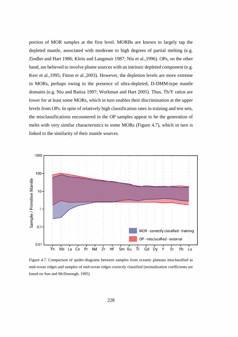
228
portion of MOR samples at the first level. MORBs are known to largely tap the
depleted mantle, associated with moderate to high degrees of partial melting (e.g.
Zindler and Hart 1986; Klein and Langmuir 1987; Niu et al.,1996). OPs, on the other
hand, are believed to involve plume sources with an intrinsic depleted component (e.g.
Kerr et al.,1995; Fitton et al.,2003). However, the depletion levels are more extreme
in MORs, perhaps owing to the presence of ultra-depleted, D-DMM-type mantle
domains (e.g. Niu and Batiza 1997; Workman and Hart 2005). Thus, Th/Y ratios are
lower for at least some MORs, which in turn enables their discrimination at the upper
levels from OPs. In spite of relatively high classification rates in training and test sets,
the misclassifications encountered in the OP samples appear to be the generation of
melts with very similar characteristics to some MORs (Figure 4.7), which in turn is
linked to the similarity of their mantle sources.
Figure 4.7. Comparison of spider-diagrams between samples from oceanic plateaus misclassified as
mid-ocean ridges and samples of mid-ocean ridges correctly classified (normalization coefficients are
based on Sun and McDonough, 1995)
229
4.2.3.3. Discrimination Between Oceanic Islands and Continental Within-plates
For training and test datasets, the first decision tree correctly classified 431 samples
of oceanic islands out of 478 with a success ratio of 90.17% at the eighth level and
345 samples of continental within-plates out of 376 with a success ratio of 91.76% at
the eighth level. Classification rates of the first decision tree in discrimination of
oceanic islands and continental within-plates are increasing for both the oceanic
islands and continental within-plates with increasing level of depth and reach to their
maximum level at the deepest level. The introduction of each level to the first decision
tree has a positive impact for discrimination of either oceanic islands or continental
within-plates or even both. Therefore, when the classification rates of first decision
tree are evaluated, the eighth level shall be preferred.
The second decision tree correctly classified 445 samples of oceanic islands out of
478 with a success ratio of 93.10% and 327 samples of continental within-plates out
of 376 with a success ratio of 86.97%. The first decision tree is more successful for
the discrimination of continental within-plates, whereas the second decision tree is
more successful for that of oceanic islands.
The classification ratios of the second decision tree are continuously increasing from
the third level to its eighth level. However, introduction of Th/Nb and Sm/Nb at fifth
level, Th/Nb, Sm/Nb, Zr/Y and Zr/Hf at sixth level, Sm/Nd, Y/Yb, Zr/Yb and Nb/Yb
at seventh level has no positive or negative effect for discrimination of either oceanic
islands or continental within-plates.
Similar to the first decision tree, when the classification rates of the second decision
tree for discrimination of oceanic islands and continental within-plates are evaluated,
the eighth level shall be preferred.
For external datasets, the first tree correctly classified 63 samples of oceanic islands
out of 237 with a success ratio of 26.25% and 251 samples of continental within-plates
out of 302 with a success ratio of 83.11%. The second decision tree is very similar to

230
the first decision tree, with only one more classification for oceanic islands. Both
decision trees fail for the discrimination of the oceanic islands for external datasets
with only 26.25% maximum success ratio at their eighth levels. The other levels have
a similar success ratio to that level. Therefore, for the classification of oceanic plateaus
in the discrimination between oceanic islands and continental within-plates,
geochemical features may not be sufficient for this external dataset with requirement
of additional information. For both decision trees, eighth levels shall be preferred
when their applicability to training and test and external datasets are evaluated, just
considering any risk of the failure for classification of oceanic plateaus for external
datasets.
The first decision tree obtained a very high success ratio for all datasets and became
successful for samples of both oceanic islands and continental within-plates in training
and test datasets.
The success ratio of this decision tree is distributed homogeneously through the
articles from different locations, with a few exceptions for the training and test
datasets. For training and test datasets, only 7 articles out of 21 having 177 samples
are classified correctly with 100% success ratio. 14 articles have misclassifications
with varying misclassification ratios.
For continental within-plates, Aviado (2015) of West Antarctic and Peate (2003) of
East Greenland, on the other hand, is correctly classified at the seventh level of the
first decision tree. Mirnejad (2006) of Leucite Hills is correctly classified at the second
level, but misclassifications are observed at higher levels. For oceanic islands,
Gurenko (2006) of Canary has misclassifications with ratio of 63%.
The overall classifications for both oceanic islands and continental within-plates are
quite high, and misclassifications are homogeneously distributed through articles for
training and datasets other than these articles, misclassifications ranging between 2%
and 35%.
231
For external datasets, only 3 articles out of 22 having 74 samples are classified
correctly with 100% success ratio. 19 articles have misclassifications with varying
misclassification ratios.
For continental within-plates, Carlson (1996) of South Brazil, Gibson (1995) of
Southeast Brazil, and Leroex (2003) of Africa can be classified correctly with
classification ratio of 100%. Endress (2011) of Egypt, Xu (2001) of SW China, and
Gibson (1997) of Trindade are articles failed at classification of the first decision tree
in discrimination between oceanic islands and continental within-plates. The other
articles have few misclassifications with relatively small misclassification ratios.
For oceanic islands, on the other hand, classification of oceanic islands failed as all
articles have major misclassifications with the misclassification ratios ranging from
34% to a complete failure of 100% for Morgan (2009) of Hawaii.
The second decision tree is similar to those obtained from the first decision tree.
The same articles have nearly the same misclassifications for all tectonic settings in
this decision tree. There are no significant changes in both classifications and
misclassifications in the second decision tree with respect to the first one. The
differences are Gibson (2000) of picrites also has misclassifications at the latest level
of this decision tree. Johnson (2005) of Siberia has much higher misclassification ratio
of 78%. Woodhead (1996) of Mangaia can be classified correctly with 100% ratio.
There are also fewer changes in misclassifications of other articles, but no other major
differences are observed between two decision trees for training and test datasets.
The classification results and ratios for the external datasets are also quite similar
between two decision trees. Gibson (1995) of Southeast Brazil and Leroex (2003) of
Africa can also be correctly classified with second decision trees.
Misclassifications also show slight fluctuations but nearly the same when compared
to that of the first decision tree.

232
The discrimination between CWP and OI probably constitutes the most challenging
classification due to compositional resemblance of lavas generated in these settings,
which arise from their derivation from similar mantle sources and under similar degree
of partial melting. Since they include no or minimal subduction component in most
cases, subduction-sensitive ratios Th/Nb and Nb/Nb* do not work at the uppermost
level. However, some CWP lavas are result of very low degree of melting under great
depths. These ones, with potassic/ultrapotassic compositions, are incredibly enriched
in incompatible elements. Thus, a ratio including a highly incompatible element and
compatible element that can be retained by garnet (like Nb/Y) can be useful for the
first order classification.
4.3. Comparison with Traditional Discrimination Methods
In this section, the decision trees are compared with traditional discrimination methods
to understand i) if there is any advantage of using them, and ii) to what extent they are
successful over the traditional methods. In fact, when the traditional methods are
considered, none of them appear to be able to discriminate all seven tectonic settings.
Such result is actually expected since the discrimination of all tectonic settings on a
single plot is extremely difficult with the limited number of elements used.
Furthermore, considering the published diagrams thus far, even their combination is
not able to distinguish all tectonic settings. Thus, in this respect, using the decision
trees can be very advantageous in the tectonomagmatic characterization of a sample
with no known affinity. Though they can be useful, the applicability of published
diagrams seems to be limited compared to the decision trees. For the discrimination
between subduction and non-subduction settings, the ternary diagram of Wood (1980)
and bivariate diagrams of Pearce (1983) and Saccani (2015) can be applied, whereas
for discrimination within subduction settings, Saccani (2015) is useful. However, no
traditional discrimination method is available for discrimination within non-
subduction settings, which can be compared with the decision trees.
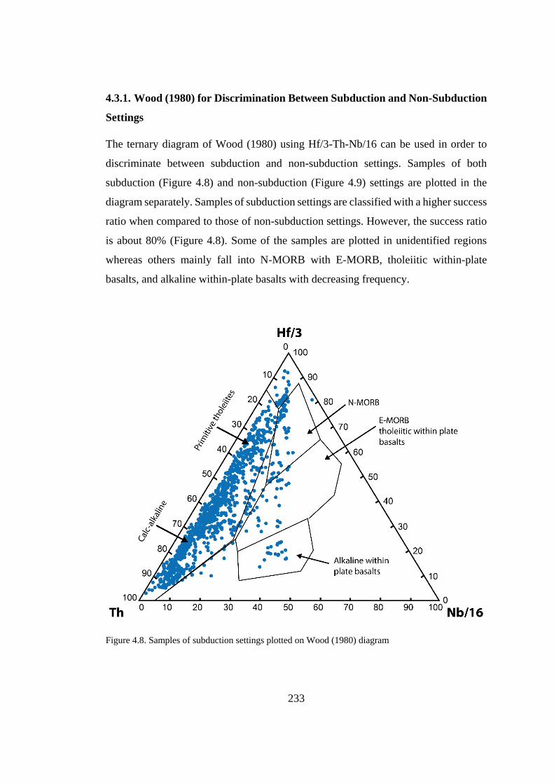
233
4.3.1. Wood (1980) for Discrimination Between Subduction and Non-Subduction
Settings
The ternary diagram of Wood (1980) using Hf/3-Th-Nb/16 can be used in order to
discriminate between subduction and non-subduction settings. Samples of both
subduction (Figure 4.8) and non-subduction (Figure 4.9) settings are plotted in the
diagram separately. Samples of subduction settings are classified with a higher success
ratio when compared to those of non-subduction settings. However, the success ratio
is about 80% (Figure 4.8). Some of the samples are plotted in unidentified regions
whereas others mainly fall into N-MORB with E-MORB, tholeiitic within-plate
basalts, and alkaline within-plate basalts with decreasing frequency.
Figure 4.8. Samples of subduction settings plotted on Wood (1980) diagram
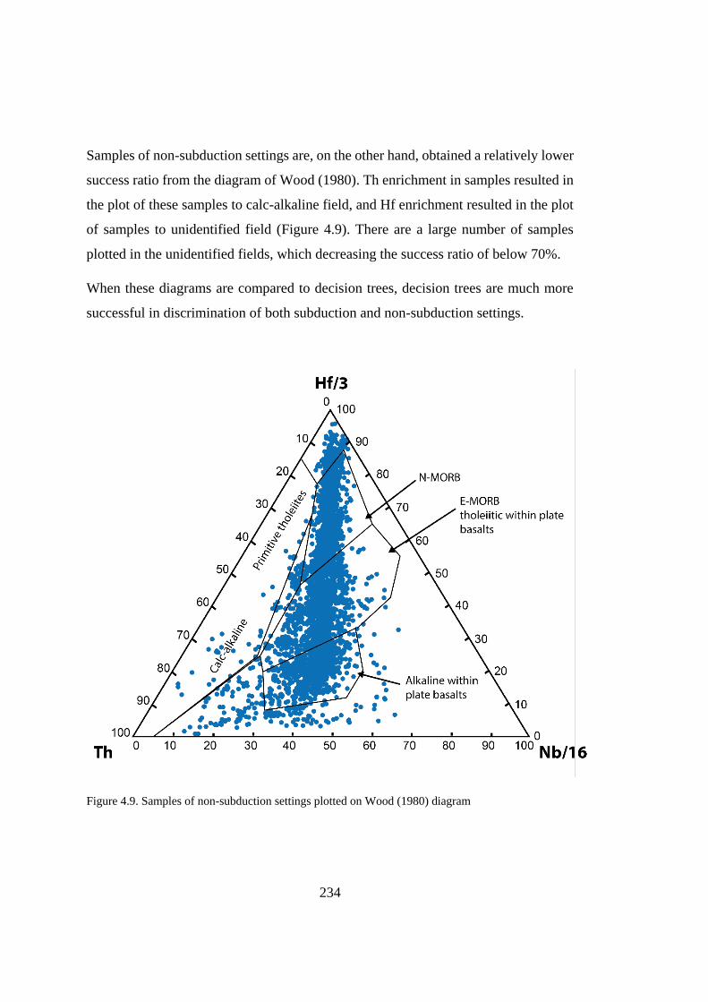
234
Samples of non-subduction settings are, on the other hand, obtained a relatively lower
success ratio from the diagram of Wood (1980). Th enrichment in samples resulted in
the plot of these samples to calc-alkaline field, and Hf enrichment resulted in the plot
of samples to unidentified field (Figure 4.9). There are a large number of samples
plotted in the unidentified fields, which decreasing the success ratio of below 70%.
When these diagrams are compared to decision trees, decision trees are much more
successful in discrimination of both subduction and non-subduction settings.
Figure 4.9. Samples of non-subduction settings plotted on Wood (1980) diagram
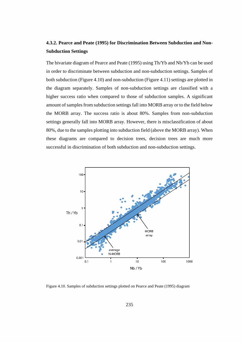
235
4.3.2. Pearce and Peate (1995) for Discrimination Between Subduction and Non-
Subduction Settings
The bivariate diagram of Pearce and Peate (1995) using Th/Yb and Nb/Yb can be used
in order to discriminate between subduction and non-subduction settings. Samples of
both subduction (Figure 4.10) and non-subduction (Figure 4.11) settings are plotted in
the diagram separately. Samples of non-subduction settings are classified with a
higher success ratio when compared to those of subduction samples. A significant
amount of samples from subduction settings fall into MORB array or to the field below
the MORB array. The success ratio is about 80%. Samples from non-subduction
settings generally fall into MORB array. However, there is misclassification of about
80%, due to the samples plotting into subduction field (above the MORB array). When
these diagrams are compared to decision trees, decision trees are much more
successful in discrimination of both subduction and non-subduction settings.
Figure 4.10. Samples of subduction settings plotted on Pearce and Peate (1995) diagram

236
Figure 4.11. Samples of non-subduction settings plotted on Pearce and Peate (1995) diagram
4.3.3. Saccani (2015) for Discrimination Between Subduction and Non-
Subduction Settings and Within Subduction Settings
Bivariate diagram of Saccani (2015) using ThN and NbN can be used in order to
discriminate between subduction and non-subduction settings. The diagram can also
be used in order to discriminate within subduction settings and to discriminate arc
settings from back-arc settings. Samples of subduction settings are plotted in the
diagram (Figure 4.12). A large amount of samples is plotted in the field defined as
divergent plate and within-plate settings. Samples of non-subduction settings are
plotted in the diagram (Figure 4.13). Saccani (2015) is relatively more successful in
discrimination of non-subduction samples with respect to subduction samples. The
samples show a linear trend in overall. However, a large amount of samples is still
misclassified as convergent plate setting (nascent forearc).
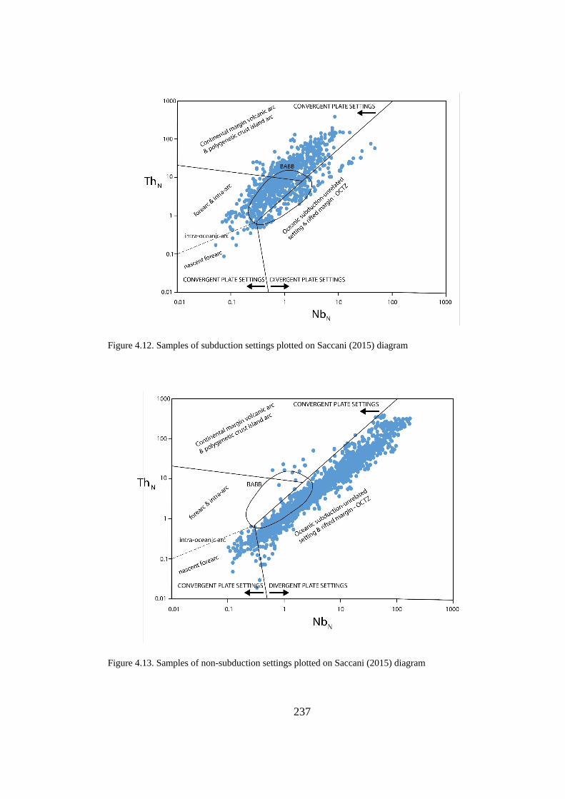
237
Figure 4.12. Samples of subduction settings plotted on Saccani (2015) diagram
Figure 4.13. Samples of non-subduction settings plotted on Saccani (2015) diagram
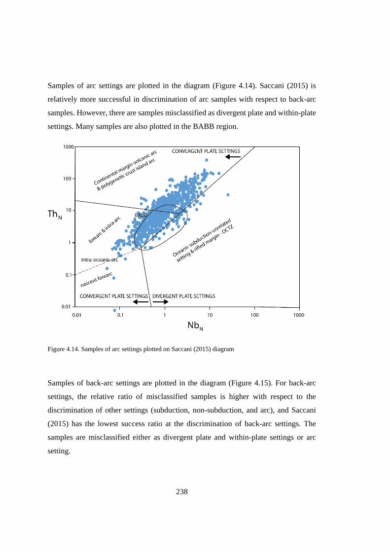
238
Samples of arc settings are plotted in the diagram (Figure 4.14). Saccani (2015) is
relatively more successful in discrimination of arc samples with respect to back-arc
samples. However, there are samples misclassified as divergent plate and within-plate
settings. Many samples are also plotted in the BABB region.
Figure 4.14. Samples of arc settings plotted on Saccani (2015) diagram
Samples of back-arc settings are plotted in the diagram (Figure 4.15). For back-arc
settings, the relative ratio of misclassified samples is higher with respect to the
discrimination of other settings (subduction, non-subduction, and arc), and Saccani
(2015) has the lowest success ratio at the discrimination of back-arc settings. The
samples are misclassified either as divergent plate and within-plate settings or arc
setting.

239
Figure 4.15. Samples of back-arc settings plotted on Saccani (2015) diagram
When these diagrams are evaluated, it can be seen that decision trees are more
successful than the traditional diagrams on the discrimination between subduction and
non-subduction settings, within subduction settings (between arc and back-arc
settings).
4.4. Recommended Decision Trees for Discriminations
4.4.1. Recommended Decision Trees for Discrimination between Subduction and
Non-Subduction
One decision stump (single-level decision tree) and two decision trees are constructed
for discrimination between subduction and non-subduction. The decision tree cannot
be longer simplified as it has only one level. It is also not necessary to simplify the
third (alternative) decision tree as it has only two levels and both levels are necessary.
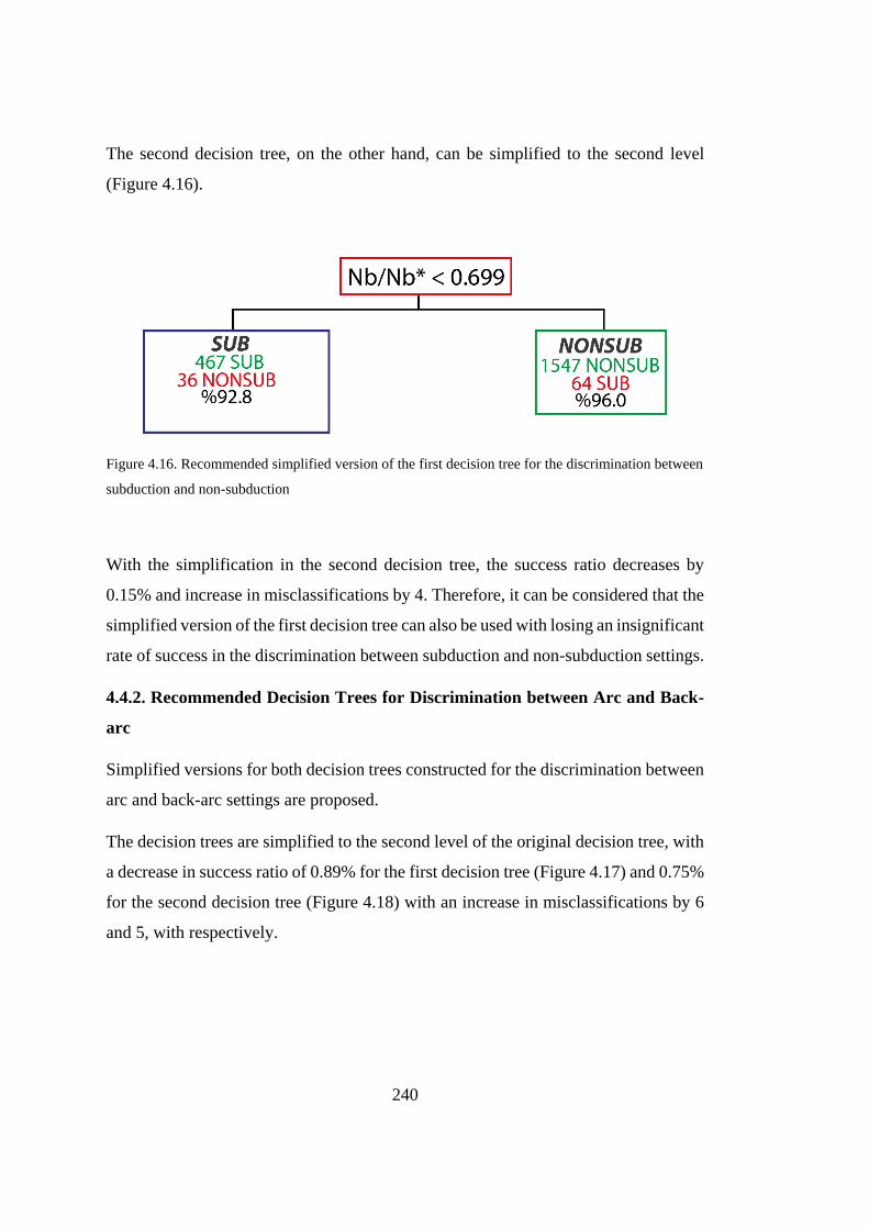
240
The second decision tree, on the other hand, can be simplified to the second level
(Figure 4.16).
Figure 4.16. Recommended simplified version of the first decision tree for the discrimination between
subduction and non-subduction
With the simplification in the second decision tree, the success ratio decreases by
0.15% and increase in misclassifications by 4. Therefore, it can be considered that the
simplified version of the first decision tree can also be used with losing an insignificant
rate of success in the discrimination between subduction and non-subduction settings.
4.4.2. Recommended Decision Trees for Discrimination between Arc and Back-
arc
Simplified versions for both decision trees constructed for the discrimination between
arc and back-arc settings are proposed.
The decision trees are simplified to the second level of the original decision tree, with
a decrease in success ratio of 0.89% for the first decision tree (Figure 4.17) and 0.75%
for the second decision tree (Figure 4.18) with an increase in misclassifications by 6
and 5, with respectively.
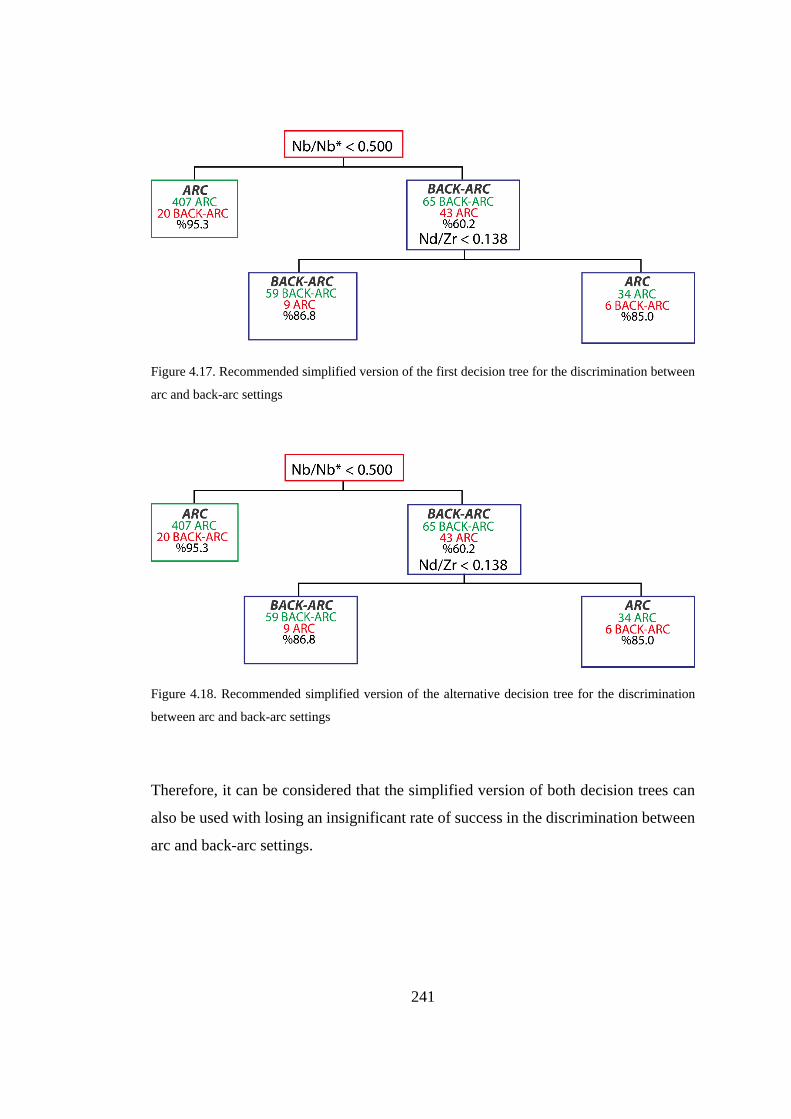
241
Figure 4.17. Recommended simplified version of the first decision tree for the discrimination between
arc and back-arc settings
Figure 4.18. Recommended simplified version of the alternative decision tree for the discrimination
between arc and back-arc settings
Therefore, it can be considered that the simplified version of both decision trees can
also be used with losing an insignificant rate of success in the discrimination between
arc and back-arc settings.

242
4.4.3. Recommended Decision Trees for Discrimination between Oceanic Arc
and Continental Arc
Simplified versions for both decision tree constructed for the discrimination between
oceanic arc and continental arc settings are proposed. The decision trees are simplified
with a decrease in success ratio of 2.66% for the first decision tree (Figure 4.19) and
8.90% for the second decision tree (Error! Reference source not found.) with an i
ncrease in misclassifications by 15 and 50, with respectively.
Therefore, it can be considered that the simplified version of both decision trees can
also be used with losing a relatively insignificant rate of success in the discrimination
between oceanic arc and continental arc settings.
4.4.4. Recommended Decision Trees for Discrimination between Oceanic and
Continental Settings
Simplified versions for both decision trees constructed for the discrimination between
arc and back-arc settings are proposed. The decision trees are simplified with a
decrease in success ratio of 7.03% for the first decision tree (Figure 4.21) and 6.28%
for the second decision tree (Figure 4.22) with an increase in misclassifications by 47
and 42, with respectively.
Therefore, it can be considered that the simplified version of both decision trees can
also be used with losing a relatively insignificant rate of success in the discrimination
between oceanic arc and continental arc settings.

243
Figure 4.19. Recommended simplified version of the first decision tree for the discrimination between Oceanic Arc and Continental Arc
Fig
ure
4.1
9.
Rec
om
men
ded
sim
pli
fied
ver
sio
n o
f th
e fi
rst
dec
isio
n t
ree
for
the
dis
crim
inat
ion
bet
wee
n O
cean
ic A
rc a
nd
Con
tin
enta
l A
rc
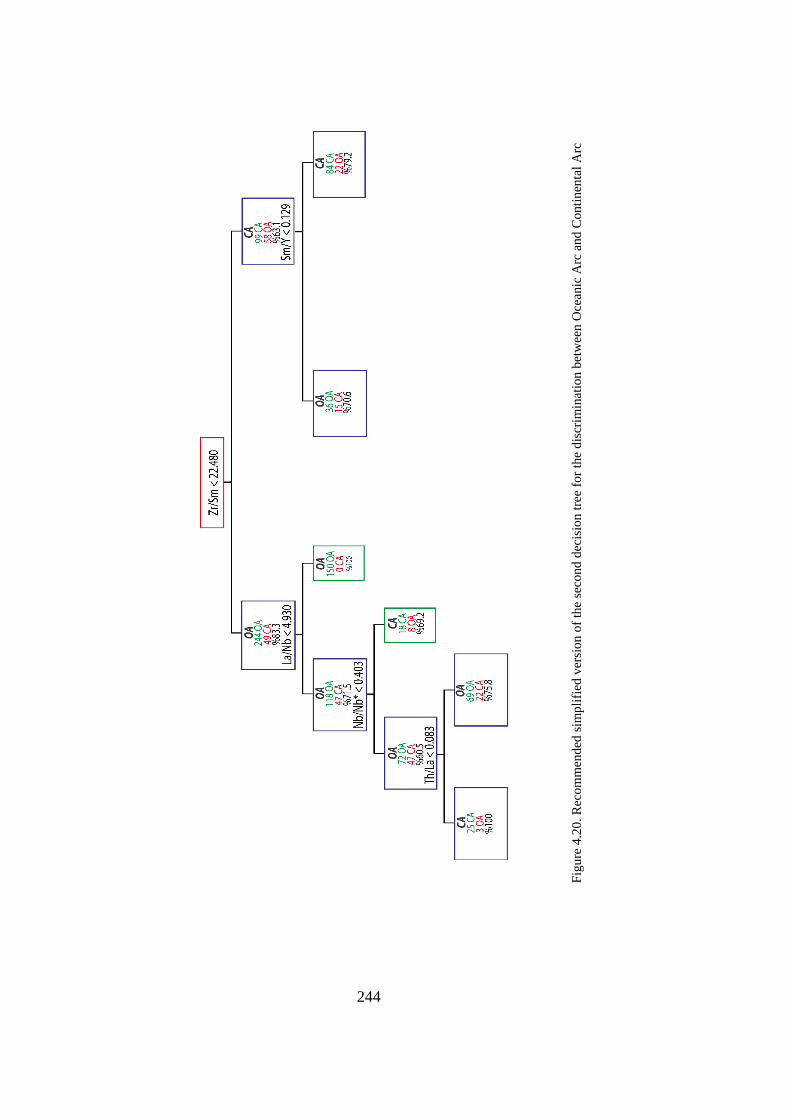
244
Figure 4.20. Recommended simplified version of the first decision tree for the discrimination between Oceanic Arc and Continental Arc
Fig
ure
4.2
0.
Rec
om
men
ded
sim
pli
fied
ver
sio
n o
f th
e se
con
d d
ecis
ion
tre
e fo
r th
e d
iscr
imin
atio
n b
etw
een
Oce
anic
Arc
an
d C
on
tin
enta
l A
rc

245
Figure 4.21. Recommended simplified version of the first decision tree for the
discrimination between oceanic and continental settings
Fig
ure
4.2
1.
Rec
om
men
ded
sim
pli
fied
ver
sio
n o
f th
e fi
rst
dec
isio
n t
ree
for
the
dis
crim
inat
ion
bet
wee
n o
cean
ic a
nd
co
nti
nen
tal
sett
ing
s
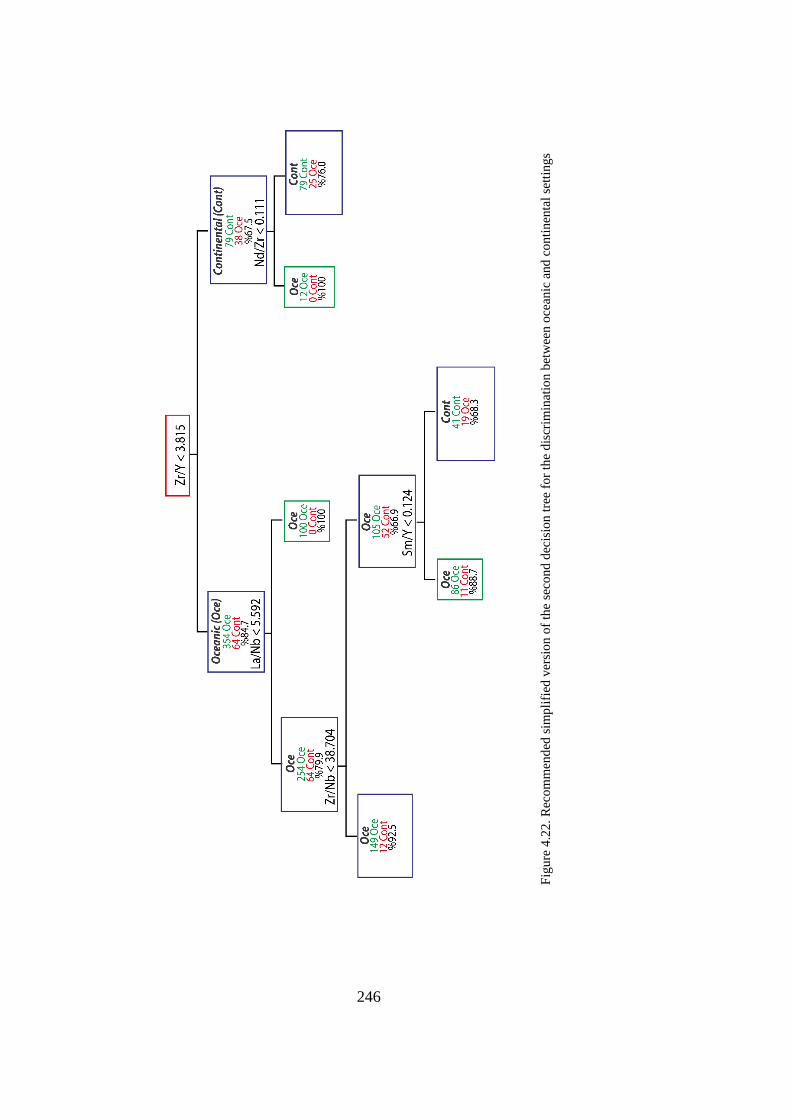
246
Figure 4.22. Recommended simplified version of the second decision tree for the discrimination between oceanic and continental settings
Fig
ure
4.2
2.
Rec
om
men
ded
sim
pli
fied
ver
sio
n o
f th
e se
con
d d
ecis
ion
tre
e fo
r th
e d
iscr
imin
atio
n b
etw
een
oce
anic
and
co
nti
nen
tal
sett
ing
s

247
4.4.5. Recommended Decision Trees for Discrimination between Oceanic Arc
and Back-arc
Only one simplified version for both decision tree (Figure 4.23) constructed for the
discrimination between oceanic arc and oceanic back-arc settings is proposed.
The decision tree is simplified with a decrease in success ratio of 7.39% for both
decision trees with an increase in misclassifications by 36.
Therefore, it can be considered that the simplified version of both decision trees can
also be used with losing a relatively insignificant rate of success in the discrimination
between oceanic and settings.
4.4.6. Recommended Decision Trees for Discrimination between Group 1 and
Group 2 of Non-Subduction Settings
Only one simplified version for both decision tree (Figure 4.24) constructed for the
discrimination between MOR+OP (Group 1) and OI+CWP (Group 2) is proposed.
The decision tree is simplified with a decrease in success ratio of 2.93% for both
decision trees with an increase in misclassifications by 58.
Therefore, it can be considered that the simplified version can also be used with losing
an insignificant rate of success in the discrimination between MOR+OP and OI+CWP.
4.4.7. Recommended Decision Trees for Discrimination between Mid-Ocean
Ridges and Oceanic Plateaus
Simplified versions for both decision trees constructed for the discrimination between
MOR and OP are proposed.
The decision trees are simplified with a decrease in success ratio of 1.96% for the first
decision tree (Figure 4.26) and 3.92% for the second decision tree (Figure 4.28) with
an increase in misclassifications by 22 and 44, with respectively.
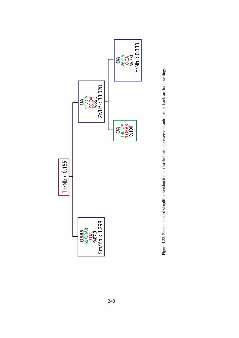
248
Figure 4.23. Recommended simplified version for the discrimination between oceanic arc and back-arc basin settings
Fig
ure
4.2
3. R
eco
mm
end
ed s
imp
lifi
ed v
ersi
on
fo
r th
e d
iscr
imin
atio
n b
etw
een o
cean
ic a
rc a
nd
bac
k-a
rc b
asin
set
tin
gs

249
Figure 4.24. Recommended simplified version of the first decision tree for the discrimination MOR+OP
and OI+CWP
Fig
ure
4.2
4. R
ecom
men
ded
sim
pli
fied
ver
sio
n o
f th
e fi
rst d
ecis
ion
tre
e fo
r th
e d
iscr
imin
atio
n M
OR
+O
P a
nd
OI+
CW
P
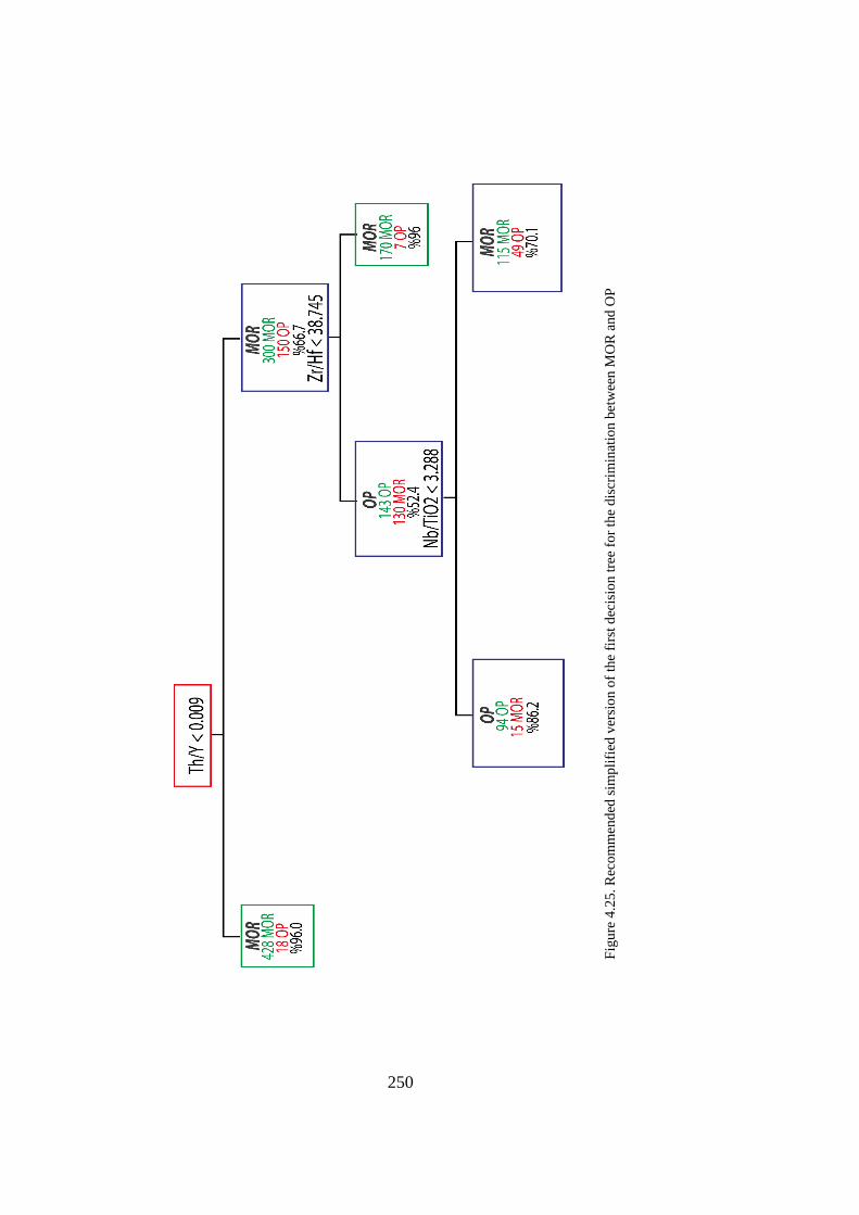
250
Figure 4.26. Recommended simplified version of the first decision tree for the discrimination between
MOR and OP
Fig
ure
4.2
5. R
ecom
men
ded
sim
pli
fied
ver
sio
n o
f th
e fi
rst
dec
isio
n t
ree
for
the
dis
crim
inat
ion
bet
wee
n M
OR
and
OP
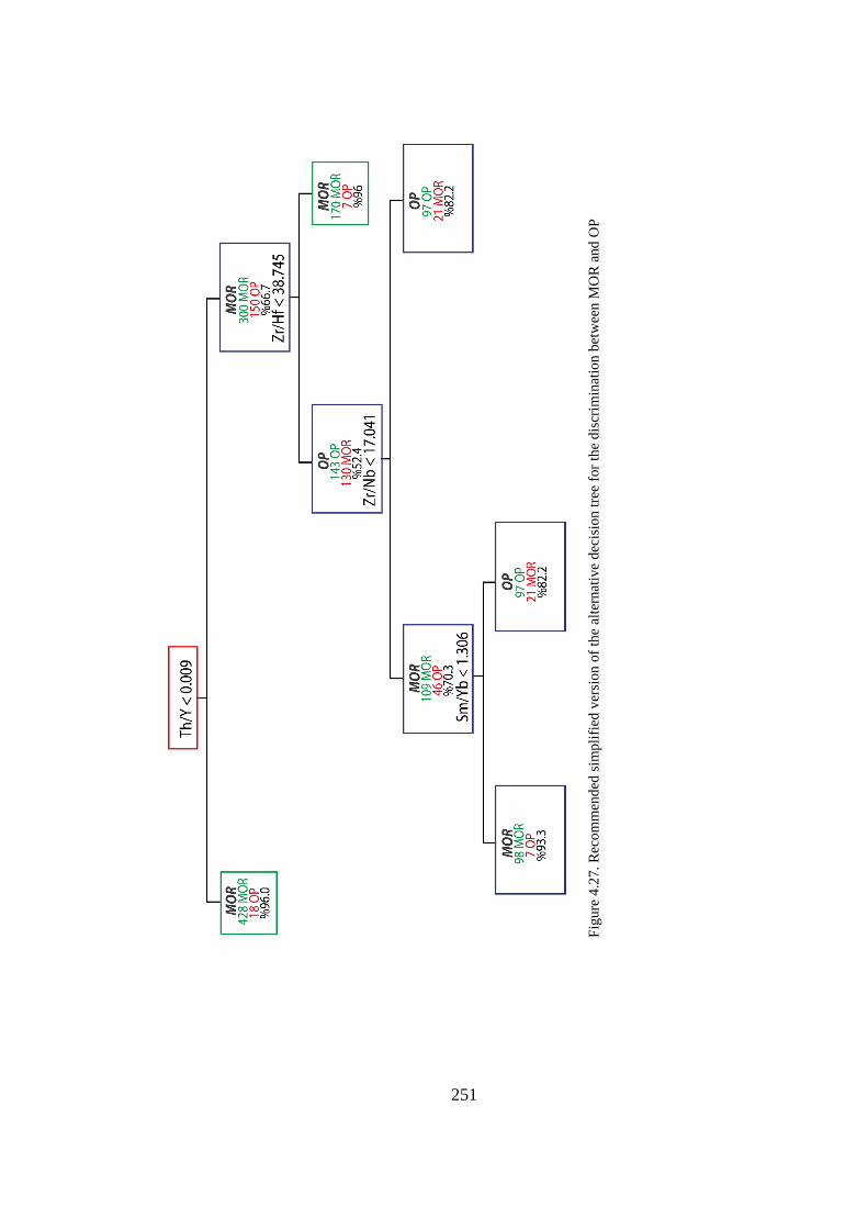
251
Figure 4.28. Recommended simplified version of the second decision tree for the discrimination between MOR and OP
Fig
ure
4.2
7.
Rec
om
men
ded
sim
pli
fied
ver
sio
n o
f th
e al
tern
ativ
e d
ecis
ion
tre
e fo
r th
e d
iscr
imin
atio
n b
etw
een
MO
R a
nd
OP

252
Therefore, it can be considered that the simplified version of both decision trees can
also be used with losing a relatively insignificant rate of success in the discrimination
between MOR and OP.
4.4.8. Recommended Decision Trees for Discrimination between Oceanic Islands
and Continental Within-Plates
Simplified versions for both decision trees constructed for the discrimination between
OI and CWP are proposed.
The decision trees are simplified with a decrease in success ratio of 4.68% for the first
decision tree (Figure 4.30) and 5.26% for the second decision tree (Figure 4.31) with
an increase in misclassifications by 40 and 45, with respectively.
Therefore, it can be considered that the simplified version of both decision trees can
also be used with losing a relatively insignificant rate of success in the discrimination
between OI and CWP.
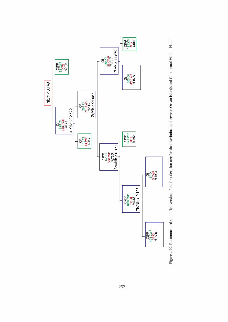
253
Figure 4.30. Recommended simplified version of the first decision tree for the discrimination between Ocean Islands and Continental Within-Plate
Fig
ure
4.2
9. R
ecom
men
ded
sim
pli
fied
ver
sio
n o
f th
e fi
rst
dec
isio
n t
ree
for
the
dis
crim
inat
ion
bet
wee
n O
cean
Isl
and
s an
d C
on
tin
enta
l W
ith
in-P
late
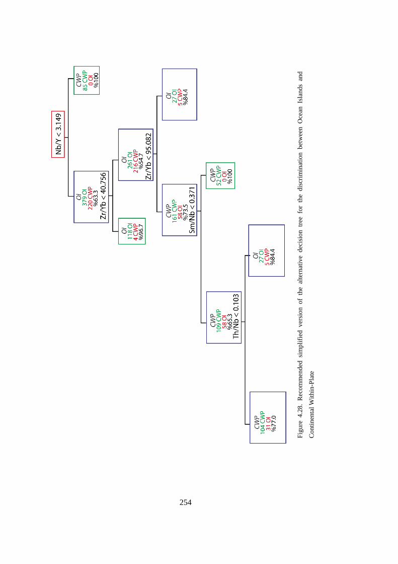
254
Figure 4.31. Recommended simplified version of the alternative decision tree for the discrimination
between Ocean Islands and Continental Within-Plate
Fig
ure
4.2
8.
Rec
om
men
ded
si
mp
lifi
ed v
ersi
on
o
f th
e al
tern
ativ
e d
ecis
ion
tr
ee fo
r th
e d
iscr
imin
atio
n b
etw
een
O
cean
Is
land
s an
d
Con
tinen
tal
Wit
hin
-Pla
te

255
CHAPTER 5
5. CONCLUSIONS
Decision trees are constructed for the tectono-magmatic discrimination of mafic
igneous rocks in order to discriminate between (1) subduction and non-subduction
settings, (2) arc-related and back-arc-related settings within subduction settings, (3)
oceanic arc and continental arc within arc-related settings, (4) oceanic and continental
settings within subduction settings, (5) oceanic arc and oceanic back-arc within
subduction-related oceanic settings, (6) mid-oceanic ridge + oceanic plateau and
oceanic island + continental within-plate within non-subduction settings, (7) mid-
oceanic ridge and oceanic plateau within non-subduction settings and (8) oceanic
island and continental within-plate within non-subduction settings.
For the discrimination between subduction and non-subduction settings, one decision
stump and two decision trees are constructed. The decision trees have 4 and 2 levels
of depth, with respectively. The element ratios used in these trees are Th/Nb, Nb/Nb*,
TiO2/Yb, Zr/Nb, La/Nb and Nb/Y. All decision trees discriminated successfully with
a success ratio of 97-99% for non-subduction and 86-88% for subduction settings.
Most journals in the dataset are correctly classified with 100% success ratio.
Within subduction settings, for discrimination between arc and back-arc-related
settings, two decision trees are constructed. The decision trees have 5 levels of depth.
The element ratios used in these trees are Nb/Nb*, Nd/Zr, TiO2/Y, Nd/TiO2, Y/Yb,
Zr/Hf, Zr/Nb, Zr/Y and Y/Yb. All decision trees discriminated successfully with a
success ratio of 98% for arc and 83-86% for back-arc-related settings. There is no
difference between two decision trees for the discrimination for arc-related settings.

256
Within arc-related settings, for discrimination between oceanic arcs and continental
arcs, two decision trees are constructed. The decision trees have 7 levels of depth. The
element ratios used in these trees are Zr/TiO2, Th/Nb, La/Nb, Nd/TiO2, Zr/Yb, La/Yb,
Y/Yb, Sm/Hf, Zr/Hf, Nb/Nb*, Zr/Sm, La/Nb, Nb/Y, Th/Y, Sm/Y, Th/La, Zr/Y, La/Y,
Sm/Nd and Zr/Nb. All decision trees discriminated successfully with a success ratio
of 97-98% for continental arcs and 92-94% for oceanic arcs.
Within subduction settings, for discrimination between oceanic and continental
settings, two decision trees are constructed. The decision trees have 6 levels of depth.
The element ratios used in these trees are Zr/Y, La/Nb, Nd/TiO2, Zr/Nb, Y/Yb,
TiO2/Y, Nb/Nb*, Zr/Hf, Sm/Hf, La/Yb, Nd/Zr and Sm/Y. All decision trees
discriminated successfully with a success ratio of 95-96% for oceanic and 83-90% for
continental settings. The second decision tree is weaker at discrimination of
continental settings.
Within subduction-related oceanic settings, for discrimination between oceanic arc
and oceanic back arcs, two decision trees are constructed. The decision trees have 6
levels of depth. The element ratios used in these trees are Th/Nb, Sm/Yb, Zr/Hf,
La/Nb, Nb/Nb*, Nd/Zr, TiO2/Yb, Y/Yb, Nb/Yb, La/Sm and Sm/Y. All decision trees
discriminated successfully with a success ratio of 99% for oceanic arcs and 92-93%
for oceanic back arcs.
Within non-subduction settings, for the discriminaton of mid-oceanic ridge and
oceanic plateau (group 1) from oceanic island and continental within-plate (group 2),
two decision trees are constructed. The decision trees have 7 levels of depth. The
element ratios used in these trees are Sm/Yb, Nd/Zr, Th/Nb, Y/Yb, Zr/TiO2, La/Nb,
Nb/Nb*, La/Sm, Nb/Yb, TiO2/Y, Zr/Hf, Th/La, Sm/Hf, Nb/Y. All decision trees
discriminated successfully with a success ratio of 96% for group 1 and 95% for group
2.

257
Within non-subduction settings, for the discriminaton of mid-ocean ridge and oceanic
plateau, two decision trees are constructed. The decision trees have 6 and 7 levels of
depth, with respectively. The element ratios used in these trees are Th/Y, Zr/Hf,
Nb/TiO2, Zr/Y, Zr/Nb, Th/La, Nb/Nb*, Sm/Yb, Sm/Y, La/Nb, Y/Yb and La/Y. All
decision trees discriminated successfully with a success ratio of 83% for oceanic
plateaus and 99% for mid-oceanic ridges. The decision trees are much more successful
for discrimination of mid-oceanic ridges.
Within non-subduction settings, for the discriminaton of oceanic island and
continental within-plate, two decision trees are constructed. The decision trees have 8
levels of depth. The element ratios used in these trees are Nb/Y, Zr/Yb, Sm/Nb, Zr/Y,
Th/Nb, TiO2/Y, Nb/TiO2, Y/Yb, Zr/Hf, Sm/Nd, Th/La, Sm/Yb, La/Y, Zr/Nb, La/Sm,
Y/Yb and Nb/Yb. All decision trees discriminated successfully with a success ratio of
90% for oceanic islands and 91% for continental within-plate.
The success ratios for external datasets are also similar to the training set for nearly
all decision trees, avoiding any risk of underfitting and overfitting. The decision trees
only fail in external datasets for the discrimination of oceanic plateau from mid-ocean
ridge (54%) and for the discrimination of continental within-plate from oceanic island
(26%). In these discriminations, two tectonic settings (oceanic plateaus and
continental within-plates) cannot be discriminated in external datasets.
A final recommendation for the decision trees is made by simplifying decision trees
to a certain level of depth in a cost of an ignorable loss in success ratio.
There are no traditional discrimination methods available in literature to discriminate
all tectonic settings included in this study. There are few diagrams discriminating
subduction settings from non-subduction settings and discriminating within
subduction setting between arc and back-arc settings. The decision trees constructed
in this study are more successful when compared to traditional methods.
Discrimination methods constructed with decision tree can only classify three tectonic

258
settings. Decision trees constructed using other modern methods such as support
vector machines or random forests tend to memorize the datasets achieving high
success ratio but tend to overfit and fail at external datasets, with different
characteristics related to training set. All modern methods use online databases such
as GeoRoc or PetDB. They also use mobile elements, isotope ratios and absolute
values of elements. Therefore, their success falls drastically in external datasets.
259
REFERENCES
Agrawal, S. (1999). Geochemical discrimination diagrams: A simple way of replacing
eye-fitted field boundaries with probability based classifier surfaces: Journal
of Geological Society of India, v. 54, p. 335–346.
Agrawal, S., and Verma, S. P. (2007). Comment on “Tectonic classification of basalts
with classification trees” by Pieter Vermeesch (2006). Geochimica et
Cosmochimica Acta, 71(13), 3388-3390.
Agrawal, S., Guevara, M., and Verma, S. P. (2004). Discriminant analysis applied to
establish major-element field boundaries for tectonic varieties of basic rocks.
International Geology Review, 46(7), 575-594.
Agrawal, S., and Verma, S. P. (2007). Comment on “Tectonic classification of basalts
with classification trees” by Pieter Vermeesch (2006). Geochimica et
Cosmochimica Acta, 71(13), 3388-3390.
Agrawal, S., Guevara, M., and Verma, S. P. (2008). Tectonic discrimination of basic
and ultrabasic volcanic rocks through log-transformed ratios of immobile
trace elements. International Geology Review, 50(12), 1057-1079.
Ahrens, L. H. (1954). The lognormal distribution of the elements (A fundamental law
of geochemistry and its subsidiary). Geochimica et Cosmochimica Acta, 5,
49-73.
Ahrens, L. H. (1954). The lognormal distribution of the elements (2). Geochimica et
cosmochimica acta, 6(2-3), 121-131.
Aitchison, J. (1981). A new approach to null correlations of proportions. Journal of
the International Association for Mathematical Geology, 13(2), 175-189.
260
Aitchison, J. (1983). Principal component analysis of compositional data. Biometrika,
70(1), 57-65.
Aitchison, J. (1984). The statistical analysis of geochemical compositions. Journal of
the International Association for Mathematical Geology, 16(6), 531-564.
Aitchison, J. (1986). A classification as a source for a thesaurus: The Bibliographic
Classification of HE Bliss as a source of thesaurus terms and structure.
Journal of documentation, 42(3), 160-181.
Aldiss, D. T. (1978). Granitic rocks of ophiolites (Doctoral dissertation, Open
University).
Armstrong-Altrin, J. S., & Verma, S. P. (2005). Critical evaluation of six tectonic
setting discrimination diagrams using geochemical data of Neogene
sediments from known tectonic settings. Sedimentary Geology, 177(1-2),
115-129.
Arevalo Jr, R., and McDonough, W. F. (2010). Chemical variations and regional
diversity observed in MOR. Chemical Geology, 271(1-2), 70-85.
Arth, J. G. (1979). Some trace elements in trondhjemites-their implications to magma
genesis and paleotectonic setting. In Developments in Petrology (Vol. 6, pp.
123-132). Elsevier.
Aviado, K. B., Rilling‐Hall, S., Bryce, J. G. and Mukasa, S. B. (2015). Submarine and
subaerial lavas in the W est A ntarctic R ift S ystem: Temporal record of
shifting magma source components from the lithosphere and asthenosphere.
Geochemistry, Geophysics, Geosystems, 16(12), 4344-4361.
Ayers, J. C. and Watson, E. B. (1993). Rutile solubility and mobility in supercritical
aqueous fluids. Contributions to Mineralogy and Petrology, 114(3), 321-330.
261
Bach, W. and Früh-Green, G. L. (2010). Alteration of the oceanic lithosphere and
implications for seafloor processes. Elements, 6(3), 173-178.
Bach, W., Peucker‐Ehrenbrink, B., Hart, S. R., and Blusztajn, J. S. (2003).
Geochemistry of hydrothermally altered oceanic crust: DSDP/ODP Hole
504B–Implications for seawater‐crust exchange budgets and Sr‐and Pb‐
isotopic evolution of the mantle. Geochemistry, Geophysics, Geosystems,
4(3).
Bailey, J. C. (1981). Geochemical criteria for a refined tectonic discrimination of
orogenic andesites. Chemical Geology, 32(1-4), 139-154.
Bailey, J. C., Jensen, E. S., Hansen, A., Kann, A. D. J., and Kann, K. (2009).
Formation of heterogeneous magmatic series beneath North Santorini, South
Aegean island arc. Lithos, 110(1-4), 20-36.
Barker, C. E. (1983). Influence of time on metamorphism of sedimentary organic
matter in liquid-dominated geothermal systems, western North America.
Geology, 11(7), 384-388.
Bédard, J. H. (1999). Petrogenesis of boninites from the Betts Cove ophiolite,
Newfoundland, Canada: identification of subducted source components.
Journal of petrology, 40(12), 1853-1889.
Beier, C., Bach, W., Turner, S., Niedermeier, D., Woodhead, J., Erzinger, J., and
Krumm, S. (2015). Origin of silicic magmas at spreading centres—an
example from the South East Rift, Manus Basin. Journal of Petrology, 56(2),
255-272.
Bézos, A., Escrig, S., Langmuir, C. H., Michael, P. J., and Asimow, P. D. (2009).
Origins of chemical diversity of back‐arc basin basalts: A segment‐scale
study of the Eastern Lau Spreading Center. Journal of Geophysical Research:
Solid Earth, 114(B6).
262
Bhatia, M. R. (1983). Plate tectonics and geochemical composition of sandstones. The
Journal of Geology, 91(6), 611-627.
Bhatia, M. R. and Crook, K. A. (1986). Trace element characteristics of graywackes
and tectonic setting discrimination of sedimentary basins. Contributions to
mineralogy and petrology, 92(2), 181-193.
Bindeman, I. N., Fournelle, J. H., and Valley, J. W. (2001). Low-δ18O tephra from a
compositionally zoned magma body: Fisher Caldera, Unimak Island,
Aleutians. Journal of Volcanology and Geothermal Research, 111(1-4), 35-
53.
Bloxam, T. W., and Lewis, A. D. (1972). Ti, Zr and Cr in some British pillow lavas
and their petrogenetic affinities. Nature physical science, 237(78), 134-136.
Bongiolo, E. M., Pires, G. L. C., Geraldes, M. C., Santos, A. C., and Neumann, R.
(2015). Geochemical modeling and Nd–Sr data links nephelinite–phonolite
successions and xenoliths of Trindade Island (South Atlantic Ocean, Brazil).
Journal of Volcanology and Geothermal Research, 306, 58-73.
Borisova, A. Y., Nikogosian, I. K., Scoates, J. S., Weis, D., Damasceno, D., Shimizu,
N., and Touret, J. L. (2002). Melt, fluid and crystal inclusions in olivine
phenocrysts from Kerguelen plume-derived picritic basalts: evidence for
interaction with the Kerguelen Plateau lithosphere. Chemical Geology,
183(1-4), 195-220.
Böttcher, W. (1969). Zur Entstehung des magmatischen Troodos-Komplexes
(Zypern). N. Jahrb. Miner. Abh., 100, 159-187
Brandl, P. A., Beier, C., Regelous, M., Abouchami, W., Haase, K. M., Garbe-
Schönberg, D., and Galer, S. J. (2012). Volcanism on the flanks of the East
Pacific Rise: Quantitative constraints on mantle heterogeneity and melting
processes. Chemical Geology, 298, 41-56.
Breiman, L. (2017). Classification and regression trees. Routledge.
263
Bryant, J. A., Yogodzinski, G. M., Hall, M. L., Lewicki, J. L., and Bailey, D. G.
(2006). Geochemical constraints on the origin of volcanic rocks from the
Andean Northern Volcanic Zone, Ecuador. Journal of petrology, 47(6), 1147-
1175.
Buccianti, A. (2013). Is compositional data analysis a way to see beyond the illusion?.
Computers and geosciences, 50, 165-173.
Butler, J. C., and Woronow, A. (1986). Discrimination among tectonic settings using
trace element abundances of basalts. Journal of Geophysical Research: Solid
Earth, 91(B10), 10289-10300.
Cabanis, B., and Lecolle, M. (1989). Le diagramme La/10eY/15eNb/8: un outil pour
la discrimination des séries volcaniques et la mise en évidence des processus
de mélange et/ou de contamination crustale. Comptes Rendus de l’Académie
des Sciences Paris, 309.
Calanchi, N., Peccerillo, A., Tranne, C. A., Lucchini, F., Rossi, P. L., Kempton, P.,
and Wu, T. W. (2002). Petrology and geochemistry of volcanic rocks from
the island of Panarea: implications for mantle evolution beneath the Aeolian
island arc (southern Tyrrhenian sea). Journal of Volcanology and Geothermal
Research, 115(3-4), 367-395.
Cann, J. R. (1970). Rb, Sr, Y, Zr and Nb in some ocean floor basaltic rocks. Earth and
Planetary Science Letters, 10(1), 7-11.
Chauvel, C., Hofmann, A. W., and Vidal, P. (1992). HIMU-EM: the French
Polynesian connection. Earth and Planetary Science Letters, 110(1-4), 99-
119.
Chayes, F. (1954). The lognormal distribution of the elements: a discussion.
Geochimica et Cosmochimica Acta, 6, 119-120.
264
Chayes, F. (1960). On correlation between variables of constant sum. Journal of
Geophysical research, 65(12), 4185-4193.
Chayes, F. (1961). Numerical petrography: Carnegie Inst. Washington Year Book, 60,
158-165.
Chayes, F. (1964). A petrographic distinction between Cenozoic volcanics in and
around the open oceans. Journal of Geophysical Research, 69(8), 1573-1588.
Chayes, F. (1965). Titania and alumina content of oceanic and circumoceanic basalt.
Mineralogical Magazine and Journal of the Mineralogical Society, 34(268),
126-131.
Chayes, F., and Velde, D. (1965). On distinguishing basaltic lavas of circum-oceanic
and oceanic-island type by means of discriminant functions. American
Journal of Science, 263(3), 206-222.
Chayes, F. (1966). Alkaline and subalkaline basalts. American Journal of Science,
264(2), 128-145.
Chayes, F. (1971). Ratio correlation: a manual for students of petrology and
geochemistry. University of Chicago Press.
Class, C., Miller, D. M., Goldstein, S. L., and Langmuir, C. H. (2000). Distinguishing
melt and fluid subduction components in Umnak Volcanics, Aleutian Arc.
Geochemistry, Geophysics, Geosystems, 1(6).
Coe, N., Le Roex, A., Gurney, J., Pearson, D. G., and Nowell, G. (2008). Petrogenesis
of the Swartruggens and Star Group II kimberlite dyke swarms, South Africa:
constraints from whole rock geochemistry. Contributions to Mineralogy and
Petrology, 156(5), 627.
Dadd, K. A., Locmelis, M., Higgins, K., and Hashimoto, T. (2011). Cenozoic
volcanism of the Capel-Faust Basins, Lord Howe Rise, SW Pacific Ocean.
265
Deep Sea Research Part II: Topical Studies in Oceanography, 58(7-8), 922-
932.
Dadd, K. A., Kellerson, L., Borissova, I., and Nelson, G. (2015). Multiple sources for
volcanic rocks dredged from the Western Australian rifted margin. Marine
Geology, 368, 42-57.
Dare, S. A., Pearce, J. A., McDonald, I., and Styles, M. T. (2009). Tectonic
discrimination of peridotites using fO2–Cr# and Ga–Ti–FeIII systematics in
chrome–spinel. Chemical Geology, 261(3-4), 199-216.
Davies, G.F., 1990. Mantle plumes, mantle stirring and hotspot chemistry. Earth and
Planetary Science Letters, 99, 94-109.
Davies, G. R., Stolz, A. J., Mahotkin, I. L., Nowell, G. M., and Pearson, D. G. (2006).
Trace element and Sr–Pb–Nd–Hf isotope evidence for ancient, fluid-
dominated enrichment of the source of Aldan Shield lamproites. Journal of
Petrology, 47(6), 1119-1146.
De Astis, G., La Volpe, L., Peccerillo, A., and Civetta, L. (1997). Volcanological and
petrological evolution of Vulcano island (Aeolian Arc, southern Tyrrhenian
Sea). Journal of Geophysical Research: Solid Earth, 102(B4), 8021-8050.
De Astis, G., Peccerillo, A., Kempton, P. D., La Volpe, L., and Wu, T. W. (2000).
Transition from calc-alkaline to potassium-rich magmatism in subduction
environments: geochemical and Sr, Nd, Pb isotopic constraints from the
island of Vulcano (Aeolian arc). Contributions to Mineralogy and Petrology,
139(6), 684-703.
Del Moro, A., Gioncada, A., Pinarelli, L., Sbrana, A., and Joron, J. L. (1998). Sr, Nd,
and Pb isotope evidence for open system evolution at Vulcano, Aeolian Arc,
Italy. Lithos, 43(2), 81-106.
266
Dilek, Y., and Furnes, H. (2009). Structure and geochemistry of Tethyan ophiolites
and their petrogenesis in subduction rollback systems. Lithos, 113(1-2), 1-
20.
Dilek, Y., Furnes, H., and Shallo, M. (2007). Geochemistry of the Jurassic Mirdita
Ophiolite (Albania) and the MORB to SSZ evolution of a marginal basin
oceanic crust. Lithos, 100(1-4), 174-209.
Dixon, J., Clague, D. A., Cousens, B., Monsalve, M. L., and Uhl, J. (2008).
Carbonatite and silicate melt metasomatism of the mantle surrounding the
Hawaiian plume: Evidence from volatiles, trace elements, and radiogenic
isotopes in rejuvenated‐stage lavas from Niihau, Hawaii. Geochemistry,
Geophysics, Geosystems, 9(9).
Eby, G. N. (1992). Chemical subdivision of the A-type granitoids: petrogenetic and
tectonic implications. Geology, 20(7), 641-644.
Egozcue, J. J., Pawlowsky-Glahn, V., Mateu-Figueras, G., and Barcelo-Vidal, C.
(2003). Isometric logratio transformations for compositional data analysis.
Mathematical Geology, 35(3), 279-300.
Elliott, T., Plank, T., Zindler, A., White, W., and Bourdon, B. (1997). Element
transport from slab to volcanic front at the Mariana arc. Journal of
Geophysical Research: Solid Earth, 102(B7), 14991-15019.
Endress, C., Furman, T., El-Rus, M. A. A., and Hanan, B. B. (2011). Geochemistry of
24 Ma basalts from NE Egypt: source components and fractionation history.
Geological Society, London, Special Publications, 357(1), 265-283.
Ewart, A. (1982). Petrogenesis of the Tertiary anorogenic volcanic series of Southern
Queensland, Australia, in the light of trace element geochemistry and O, Sr
and Pb isotopes. Journal of Petrology, 23(3), 344-382.
Finney, B., Turner, S., Hawkesworth, C., Larsen, J., Nye, C., George, R., and
Eichelberger, J. (2008). Magmatic differentiation at an island-arc caldera:
267
Okmok Volcano, Aleutian Islands, Alaska. Journal of Petrology, 49(5), 857-
884.
Fitton, J. G., and Godard, M. (2004). Origin and evolution of magmas on the Ontong
Java Plateau. Geological Society, London, Special Publications, 229(1), 151-
178.
Floyd, P. A. and Winchester, J.A. (1975). Magma Type and Tectonic Setting
Discrimination Using Immobile Elements. Earth and Planetary Science
Letters, 27, 211-218
Frey, F. A., McNaughton, N. J., Nelson, D. R., and Duncan, R. A. (1996). Petrogenesis
of the Bunbury Basalt, Western Australia: interaction between the Kerguelen
plume and Gondwana lithosphere?. Earth and Planetary Science Letters,
144(1-2), 163-183.
Frey, F. A., Weis, D., Borisova, A. Y., and Xu, G. (2002). Involvement of continental
crust in the formation of the Cretaceous Kerguelen Plateau: new perspectives
from ODP Leg 120 sites. Journal of Petrology, 43(7), 1207-1239.
Furman, T., Bryce, J.G., Karson, J., and Iotti, A., 2004. East African Rift System
(EARS) plume structure: Insights from Quaternary mafic lavas of Turkana,
Kenya. Journal of Petrology, 45, 1069-1088.
Furman, T., Bryce, J., Rooney, T., Hanan, B., Yirgu, G. and Ayalew, D. (2006). Heads
and tails: 30 million years of the Afar Plume, Geological Society, London,
Special Publications, 259, 95-119
Gale, A., Escrig, S., Gier, E. J., Langmuir, C. H., and Goldstein, S. L. (2011). Enriched
basalts at segment centers: The Lucky Strike (37 17′ N) and Menez Gwen
(37 50′ N) segments of the Mid‐Atlantic Ridge. Geochemistry, Geophysics,
Geosystems, 12(6).
268
Geldmacher, J., and Hoernle, K. (2000). The 72 Ma geochemical evolution of the
Madeira hotspot (eastern North Atlantic): recycling of Paleozoic (≤ 500 Ma)
oceanic lithosphere. Earth and Planetary Science Letters, 183(1-2), 73-92.
Gertisser, R., and Keller, J. (2000). From basalt to dacite: origin and evolution of the
calc-alkaline series of Salina, Aeolian Arc, Italy. Contributions to
Mineralogy and Petrology, 139(5), 607-626.
Gibson, S. A., Thompson, R. N., Leat, P.T., Morrison, M.A., Hendry, G.L., Dickin,
A. P. and Mitchell, J.P., (1993), Oligo-Miocene Rio Grande Rift, USA:
Monitors of the Zone of Lithospheric Mantle Extension and Thinning
Beneath a Continental Rift, Journal of Petrology, 34, 1, 187-228
Gibson, S. A., Thompson, R. N., Leonardos, O. H., Dickin, A. P., and Mitchell, J. G.
(1995). The Late Cretaceous impact of the Trindade mantle plume: evidence
from large-volume, mafic, potassic magmatism in SE Brazil. Journal of
Petrology, 36(1), 189-229.
Gibson, S.A., Thompson, R.N., Dickin, A.P. and Leonards, O.H. (1995). High-Ti and
low-Ti mafic potassic magmas: Key to plume-lithosphere interactions and
continental flood-basalt genesis, Earth and Planetary Science Letters, 136,
149-165
Gibson, S.A., Thompson, R.N., Weska, R.K., Dickin, A.P. and Leonards, O.H. (1997).
Late Cretaceous Rift-Related Upwelling and Melting of the Trindade Starting
Mantle Plume Head Beneath Western Brazil, Contrib. Mineral. Petrol. 126,
303-314
Gibson, S. A., Thompson, R. N., and Dickin, A. P. (2000). Ferropicrites: geochemical
evidence for Fe-rich streaks in upwelling mantle plumes. Earth and Planetary
Science Letters, 174(3-4), 355-374.
Gibson, S. A., Thompson, R. N., Day, J. A., Humphris, S. E., and Dickin, A. P. (2005).
Melt-generation processes associated with the Tristan mantle plume:
Constraints on the origin of EM-1. Earth and Planetary Science Letters,
237(3-4), 744-767.
269
Gorton, M. P., and Schandl, E. S. (2000). From continents to island arcs: a
geochemical index of tectonic setting for arc-related and within-plate felsic
to intermediate volcanic rocks. The Canadian Mineralogist, 38(5), 1065-
1073.
Gurenko, A. A., Hoernle, K. A., Hauff, F., Schmincke, H. U., Han, D., Miura, Y. N.,
and Kaneoka, I. (2006). Major, trace element and Nd–Sr–Pb–O–He–Ar
isotope signatures of shield stage lavas from the central and western Canary
Islands: insights into mantle and crustal processes. Chemical Geology,
233(1-2), 75-112.
Haase, K. M., Devey, C. W., and Wieneke, M. (2003). Magmatic processes and mantle
heterogeneity beneath the slow-spreading northern Kolbeinsey Ridge
segment, North Atlantic. Contributions to Mineralogy and Petrology, 144(4),
428-448.
Hastie, A. R., Kerr, A. C., Pearce, J. A., and Mitchell, S. F. (2007). Classification of
altered volcanic island arc rocks using immobile trace elements: development
of the Th–Co discrimination diagram. Journal of petrology, 48(12), 2341-
2357.
Hastie, A. R., Fitton, J. G., Kerr, A. C., McDonald, I., Schwindrofska, A., & Hoernle,
K. (2016). The composition of mantle plumes and the deep Earth. Earth and
Planetary Science Letters, 444, 13-25.
Hamelin, C., Dosso, L., Hanan, B., Barrat, J. A., and Ondréas, H. (2010). Sr‐Nd‐Hf
isotopes along the Pacific Antarctic Ridge from 41 to 53° S. Geophysical
Research Letters, 37(10).
Hanghøj, K., Storey, M., and Stecher, O. (2003). An isotope and trace element study
of the East Greenland Tertiary dyke swarm: constraints on temporal and
spatial evolution during continental rifting. Journal of Petrology, 44(11),
2081-2112.
270
Hanyu, T., Tatsumi, Y., Senda, R., Miyazaki, T., Chang, Q., Hirahara, Y., and Nakai,
S. I. (2011). Geochemical characteristics and origin of the HIMU reservoir:
A possible mantle plume source in the lower mantle. Geochemistry,
Geophysics, Geosystems, 12(2).
Harris, M., Le Roex, A., and Class, C. (2004). Geochemistry of the Uintjiesberg
kimberlite, South Africa: petrogenesis of an off-craton, group I, kimberlite.
Lithos, 74(3-4), 149-165.
Harrison, D., Leat, P. T., Burnard, P. G., Turner, G., Fretzdorff, S., and Millar, I. L.
(2003). Resolving mantle components in oceanic lavas from segment E2 of
the East Scotia back-arc ridge, South Sandwich Islands. Geological Society,
London, Special Publications, 219(1), 333-344.
Hastie, A. R., Kerr, A. C., Pearce, J. A., and Mitchell, S. F. (2007). Classification of
altered volcanic island arc rocks using immobile trace elements: development
of the Th–Co discrimination diagram. Journal of petrology, 48(12), 2341-
2357.
Hastie, A. R., Fitton, J. G., Kerr, A. C., McDonald, I., Schwindrofska, A., and Hoernle,
K. (2016). The composition of mantle plumes and the deep Earth. Earth and
Planetary Science Letters, 444, 13-25.
Hickey‐Vargas, R. (1998). Origin of the Indian Ocean‐type isotopic signature in
basalts from Philippine Sea plate spreading centers: An assessment of local
versus large‐scale processes. Journal of Geophysical Research: Solid Earth,
103(B9), 20963-20979.
Hickey-Vargas, R., Bizimis, M., and Deschamps, A. (2008). Onset of the Indian
Ocean isotopic signature in the Philippine Sea Plate: Hf and Pb isotope
evidence from Early Cretaceous terranes. Earth and Planetary Science
Letters, 268(3-4), 255-267.
Hickey-Vargas, R., Ishizuka, O., and Bizimis, M. (2013). Age and geochemistry of
volcanic clasts from DSDP Site 445, Daito Ridge and relationship to Minami-
271
Daito Basin and early Izu-Bonin arc magmatism. Journal of Asian Earth
Sciences, 70, 193-208.
Hickey-Vargas, R., Holbik, S., Tormey, D., Frey, F. A., and Roa, H. M. (2016).
Basaltic rocks from the Andean Southern Volcanic Zone: Insights from the
comparison of along-strike and small-scale geochemical variations and their
sources. Lithos, 258, 115-132.
Hickey-Vargas, R., Sun, M., and Holbik, S. (2016). Geochemistry of basalts from
small eruptive centers near Villarrica stratovolcano, Chile: evidence for
lithospheric mantle components in continental arc magmas. Geochimica et
Cosmochimica Acta, 185, 358-382.
Hochstaedter, A., Gill, J., Peters, R., Broughton, P., Holden, P., and Taylor, B. (2001).
Across‐arc geochemical trends in the Izu‐Bonin arc: Contributions from the
subducting slab. Geochemistry, Geophysics, Geosystems, 2(7).
Hoernle, K., Hauff, F., Kokfelt, T. F., Haase, K., Garbe-Schönberg, D., and Werner,
R. (2011). On-and off-axis chemical heterogeneities along the South Atlantic
Mid-Ocean-Ridge (5–11° S): shallow or deep recycling of ocean crust and/or
intraplate volcanism?. Earth and Planetary Science Letters, 306(1-2), 86-97.
Hoernle, K., van den Bogaard, P., Duggen, S., Mocek, B., and Garbe-Schönberg, D.
(1999). Evidence for Miocene subduction beneath the Alboran Sea (Western
Mediterranean) from 40Ar/39Ar age dating and the geochemistry of volcanic
rocks from holes 977A and 978A. Ocean Drilling Project.
Hollocher, K., Bull, J., and Robinson, P. (2012). Geochemistry of the metamorphosed
Ordovician Taconian magmatic arc, Bronson Hill anticlinorium, western
New England. Physics and Chemistry of the Earth, Parts A/B/C, 27(1-3), 5-
45.
Iannelli, S. B., Litvak, V. D., Paz, L. F., Folguera, A., Ramos, M. E., and Ramos, V.
A. (2017). Evolution of Eocene to Oligocene arc-related volcanism in the
North Patagonian Andes (39–41 S), prior to the break-up of the Farallon
plate. Tectonophysics, 696, 70-87.
272
Ikeda, Y., Nagao, K., Ishii, T., Matsumoto, D., Stern, R. J., Kagami, H., and Bloomer,
S. H. (2016). Contributions of slab fluid and sediment melt components to
magmatism in the Mariana Arc–Trough system: Evidence from geochemical
compositions and Sr, Nd, and noble gas isotope systematics. Island Arc,
25(4), 253-273.
Irvine, T. N. J., and Baragar, W. R. A. (1971). A guide to the chemical classification
of the common volcanic rocks. Canadian journal of earth sciences, 8(5), 523-
548.
Ishizuka, O., Taylor, R. N., Milton, J. A., and Nesbitt, R. W. (2003). Fluid–mantle
interaction in an intra-oceanic arc: constraints from high-precision Pb
isotopes. Earth and Planetary Science Letters, 211(3-4), 221-236.
Ishizuka, O., Yuasa, M., Taylor, R. N., and Sakamoto, I. (2009). Two contrasting
magmatic types coexist after the cessation of back-arc spreading. Chemical
Geology, 266(3-4), 274-296.
Jackson, M. G., Hart, S. R., Konter, J. G., Koppers, A. A., Staudigel, H., Kurz, M. D.,
and Sinton, J. M. (2010). Samoan hot spot track on a “hot spot highway”:
Implications for mantle plumes and a deep Samoan mantle source.
Geochemistry, Geophysics, Geosystems, 11(12).
Janney, P. E., Le Roex, A. P., Carlson, R. W., and Viljoen, K. S. (2002). A chemical
and multi-isotope study of the Western Cape olivine melilitite province,
South Africa: implications for the sources of kimberlites and the origin of the
HIMU signature in Africa. Journal of Petrology, 43(12), 2339-2370.
Jenner, F. E., and O'Neill, H. S. C. (2012). Analysis of 60 elements in 616 ocean floor
basaltic glasses. Geochemistry, Geophysics, Geosystems, 13(2).
Johnson, J. S., Gibson, S. A., Thompson, R. N., and Nowell, G. M. (2005). Volcanism
in the Vitim volcanic field, Siberia: geochemical evidence for a mantle plume
beneath the Baikal rift zone. Journal of Petrology, 46(7), 1309-1344.
273
Jolly, W. T., Schellekens, J. H., and Dickin, A. P. (2007). High-Mg andesites and
related lavas from southwest Puerto Rico (Greater Antilles Island Arc):
Petrogenetic links with emplacement of the Late Cretaceous Caribbean
mantle plume. Lithos, 98(1-4), 1-26.
Jolly, W. T., Lidiak, E. G., and Dickin, A. P. (2008). The case for persistent southwest-
dipping Cretaceous convergence in the northeast Antilles: Geochemistry,
melting models, and tectonic implications. Geological Society of America
Bulletin, 120(7-8), 1036-1052.
Jolly, W. T., Lidiak, E. G., and Dickin, A. P. (2008). Bimodal volcanism in northeast
Puerto Rico and the Virgin Islands (Greater Antilles Island Arc): Genetic
links with Cretaceous subduction of the mid-Atlantic ridge Caribbean spur.
Lithos, 103(3-4), 393-414.
Kelley, K. A., Kingsley, R., and Schilling, J. G. (2013). Composition of plume‐
influenced mid‐ocean ridge lavas and glasses from the Mid‐Atlantic Ridge,
East Pacific Rise, Galápagos Spreading Center, and Gulf of Aden.
Geochemistry, Geophysics, Geosystems, 14(1), 223-242.
Kempton, P. D., Fitton, J. G., Saunders, A. D., Nowell, G. M., Taylor, R. N.,
Hardarson, B. S., and Pearson, G. (2000). The Iceland plume in space and
time: a Sr–Nd–Pb–Hf study of the North Atlantic rifted margin. Earth and
Planetary Science Letters, 177(3-4), 255-271.
Kempton, P. D., Pearce, J. A., Barry, T. L., Fitton, J. G., Langmuir, C., and Christie,
D. M. (2002). Sr‐Nd‐Pb‐Hf isotope results from ODP Leg 187: Evidence for
mantle dynamics of the Australian‐Antarctic discordance and origin of the
Indian MOR source. Geochemistry, Geophysics, Geosystems, 3(12), 1-35.
Kitagawa, H., Kobayashi, K., Makishima, A., and Nakamura, E. (2008). Multiple
pulses of the mantle plume: evidence from Tertiary Icelandic lavas. Journal
of Petrology, 49(7), 1365-1396.
274
Kokfelt, T. F., Hoernle, K. A. J., Hauff, F., Fiebig, J., Werner, R., and Garbe-
Schönberg, D. (2006). Combined trace element and Pb-Nd–Sr-O isotope
evidence for recycled oceanic crust (upper and lower) in the Iceland mantle
plume. Journal of Petrology, 47(9), 1705-1749.
König, S., Münker, C., Schuth, S., and Garbe-Schönberg, D. (2008). Mobility of
tungsten in subduction zones. Earth and Planetary Science Letters, 274(1-2),
82-92.
König, S., Münker, C., Schuth, S., Luguet, A., Hoffmann, J. E., and Kuduon, J. (2010).
Boninites as windows into trace element mobility in subduction zones.
Geochimica et Cosmochimica Acta, 74(2), 684-704.
Kuno, H. (1960). High-alumina basalt. Journal of petrology, 1(1), 121-145.
Kushiro, I., and Kuno, H. (1963). Origin of primary basalt magmas and classification
of basaltic rocks. Journal of Petrology, 4(1), 75-89.
Larsen, L. M., Pedersen, A. K., Sundvoll, B., and Freı, R. (2003). Alkali picrites
formed by melting of old metasomatized lithospheric mantle: Manitdlat
Member, Vaigat Formation, Palaeocene of West Greenland. Journal of
Petrology, 44(1), 3-38.
Lassiter, J. C., Blichert-Toft, J., Hauri, E. H., and Barsczus, H. G. (2003). Isotope and
trace element variations in lavas from Raivavae and Rapa, Cook–Austral
islands: constraints on the nature of HIMU-and EM-mantle and the origin of
mid-plate volcanism in French Polynesia. Chemical Geology, 202(1-2), 115-
138.
Le Bas, M., Maitre, R. L., Streckeisen, A., Zanettin, B., and IUGS Subcommission on
the Systematics of Igneous Rocks. (1986). A chemical classification of
volcanic rocks based on the total alkali-silica diagram. Journal of petrology,
27(3), 745-750.
275
LeRoex, A. P., and Lanyon, R. (1998). Isotope and trace element geochemistry of
Cretaceous Damaraland lamprophyres and carbonatites, northwestern
Namibia: Evidence for plume—lithosphere interactions. Journal of
Petrology, 39(6), 1117-1146.
LeRoex, A. P., Bell, D. R., and Davis, P. (2003). Petrogenesis of group I kimberlites
from Kimberley, South Africa: evidence from bulk-rock geochemistry.
Journal of Petrology, 44(12), 2261-2286.
Leat, P. T., Livermore, R. A., Millar, I. L., and Pearce, J. A. (2000). Magma supply in
back-arc spreading centre segment E2, East Scotia Ridge. Journal of
Petrology, 41(6), 845-866.
Leat, P. T., Pearce, J. A., Barker, P. F., Millar, I. L., Barry, T. L., and Larter, R. D.
(2004). Magma genesis and mantle flow at a subducting slab edge: the South
Sandwich arc-basin system. Earth and Planetary Science Letters, 227(1-2),
17-35.
Leslie, R. A., Danyushevsky, L. V., Crawford, A. J., and Verbeeten, A. C. (2009).
Primitive shoshonites from Fiji: Geochemistry and source components.
Geochemistry, Geophysics, Geosystems, 10(7).
Li, C., Arndt, N. T., Tang, Q., and Ripley, E. M. (2015). Trace element
indiscrimination diagrams. Lithos, 232, 76-83.
Mana, S., Furman, T., Turrin, B. D., Feigenson, M. D., and Swisher III, C. C. (2015).
Magmatic activity across the East African North Tanzanian Divergence
Zone. Journal of the Geological Society, 172(3), 368-389.
Martinez, F., and Taylor, B. (2002). Mantle wedge control on back-arc crustal
accretion. Nature, 416(6879), 417.
Martinez, F., and Taylor, B. (2006). Modes of crustal accretion in back-arc basins:
Inferences from the Lau Basin. Washington DC American Geophysical
Union Geophysical Monograph Series, 166, 5-30.
276
McKenzie, D., and O’Nions, R.K., 1991. Partial melt distributions from inversion of
rare earth element concentrations. Journal of Petrology, 32, 1021-1091.
Meschede, M. (1986). A method of discriminating between different types of mid-
ocean ridge basalts and continental tholeiites with the Nb 1bZr 1bY
diagram. Chemical geology, 56(3-4), 207-218.
Métrich, N., Bertagnini, A., Landi, P., and Rosi, M. (2001). Crystallization driven by
decompression and water loss at Stromboli volcano (Aeolian Islands, Italy).
Journal of Petrology, 42(8), 1471-1490.
Millet, M. A., Doucelance, R., Baker, J. A., and Schiano, P. (2009). Reconsidering the
origins of isotopic variations in Ocean Island Basalts: insights from fine-scale
study of São Jorge Island, Azores archipelago. Chemical Geology, 265(3-4),
289-302.
Mirnejad, H., and Bell, K. (2006). Origin and source evolution of the Leucite Hills
lamproites: evidence from Sr–Nd–Pb–O isotopic compositions. Journal of
Petrology, 47(12), 2463-2489.
Miyashiro, A. (1973). The Troodos ophiolitic complex was probably formed in an
island arc. Earth and Planetary Science Letters, 19(2), 218-224.
Miyashiro, A. (1974). Volcanic rock series in island arcs and active continental
margins. American journal of science, 274(4), 321-355.
Miyashiro, A. (1975). Origin of the Troodos and other ophiolites: a reply to Hynes.
Earth and planetary science letters, 25(2), 217-222.
Miyashiro, A., and Shido, F. (1975). Tholeiitic and calc-alkalic series in relation to
the behaviors of titanium, vanadium, chromium, and nickel. American
Journal of Science, 275(3), 265-277.

277
Moores, E. M., and Vine, F. J. (1971). The Troodos Massif, Cyprus and other
ophiolites as oceanic crust: evaluation and implications. Philosophical
Transactions of the Royal Society of London. Series A, Mathematical and
Physical Sciences, 268(1192), 443-467.
Morgan, J. K., Clague, D. A., Borchers, D. C., Davis, A. S., and Milliken, K. L. (2007).
Mauna Loa's submarine western flank: Landsliding, deep volcanic spreading,
and hydrothermal alteration. Geochemistry, Geophysics, Geosystems, 8(5).
Morimoto, N. (1988). Nomenclature of pyroxenes. Mineralogy and Petrology, 39(1),
55-76.
Mortimer, N., Herzer, R. H., Gans, P. B., Laporte-Magoni, C., Calvert, A. T., and
Bosch, D. (2007). Oligocene–Miocene tectonic evolution of the South Fiji
Basin and Northland Plateau, SW Pacific Ocean: Evidence from petrology
and dating of dredged rocks. Marine Geology, 237(1-2), 1-24.
Mullen, E. D. (1983). MnO/TiO2/P2O5: a minor element discriminant for basaltic
rocks of oceanic environments and its implications for petrogenesis. Earth
and Planetary Science Letters, 62(1), 53-62.
Mullen, E. K., Weis, D., Marsh, N. B., and Martindale, M. (2017). Primitive arc
magma diversity: New geochemical insights in the Cascade Arc. Chemical
Geology, 448, 43-70.
Mullen, E. K., and Weis, D. (2015). Evidence for trench-parallel mantle flow in the
northern Cascade Arc from basalt geochemistry. Earth and Planetary Science
Letters, 414, 100-107.
Muravyeva, N. S., Belyatsky, B. V., Senin, V. G., and Ivanov, A. V. (2014). Sr–Nd–
Pb isotope systematics and clinopyroxene-host disequilibrium in ultra-
potassic magmas from Toro-Ankole and Virunga, East-African Rift:
Implications for magma mixing and source heterogeneity. Lithos, 210, 260-
277.
278
Murton, B. J., Peate, D. W., Arculus, R. J., Pearce, J. A., and Van der Laan, S. (1992).
12. Trace-Element Geochemistry Of Volcanic Rocks From Site 786: The Izu-
Bonin Forearc1. In Proceedings of the Ocean Drilling Program, scientific
results (Vol. 125, pp. 211-235).
Nauret, F., Abouchami, W., Galer, S. J. G., Hofmann, A. W., Hémond, C., Chauvel,
C., and Dyment, J. (2006). Correlated trace element-Pb isotope enrichments
in Indian MOR along 18–20 S, Central Indian Ridge. Earth and Planetary
Science Letters, 245(1-2), 137-152.
Neal, C. R., Mahoney, J. J., and Chazey III, W. J. (2002). Mantle sources and the
highly variable role of continental lithosphere in basalt petrogenesis of the
Kerguelen Plateau and Broken Ridge LIP: results from ODP Leg 183. Journal
of Petrology, 43(7), 1177-1205.
Niu, Y. and Batiza, R. (1997). Trace element evidence from seamounts for recycled
oceanic crust in the Eastern Pacific mantle. Earth and Planetary Science
Letters, 148(3-4), 471-483.
Niu, Y., Collerson, K. D., Batiza, R., Wendt, J. I., and Regelous, M. (1999). Origin of
enriched‐type mid‐ocean ridge basalt at ridges far from mantle plumes: The
East Pacific Rise at 11 20′ N. Journal of Geophysical Research: Solid Earth,
104(B4), 7067-7087.
Niu, Y., Regelous, M., Wendt, I. J., Batiza, R., and O’Hara, M. J. (2002).
Geochemistry of near-EPR seamounts: importance of source vs. process and
the origin of enriched mantle component. Earth and Planetary Science
Letters, 199(3-4), 327-345.
Olierook, H. K., Jourdan, F., Merle, R. E., Timms, N. E., Kusznir, N., and Muhling,
J. R. (2016). Bunbury Basalt: Gondwana breakup products or earliest
vestiges of the Kerguelen mantle plume?. Earth and Planetary Science
Letters, 440, 20-32.
279
Pandarinath, K., Dulski, P., Torres-Alvarado, I. S., and Verma, S. P. (2008). Element
mobility during the hydrothermal alteration of rhyolitic rocks of the Los
Azufres geothermal field, Mexico. Geothermics, 37(1), 53-72.
Pandarinath, K., and Verma, S. K. (2013). Application of four sets of tectonomagmatic
discriminant function based diagrams to basic rocks from northwest Mexico.
Journal of Iberian Geology, 39(1), 181-195.
Pandarinath, K. (2014). Testing of the recently developed tectonomagmatic
discrimination diagrams from hydrothermally altered igneous rocks of 7
geothermal fields. Turkish Journal of Earth Sciences, 23(4), 412-426.
Panter, K. S., Blusztajn, J., Hart, S. R., Kyle, P. R., Esser, R., and McIntosh, W. C.
(2006). The origin of HIMU in the SW Pacific: evidence from intraplate
volcanism in southern New Zealand and subantarctic islands. Journal of
Petrology, 47(9), 1673-1704.
Pawlowsky-Glahn, V., and Egozcue, J. J. (2006). Compositional data and their
analysis: an introduction. Geological Society, London, Special Publications,
264(1), 1-10.
Pearce, J.A., 1975. Basalt geochemistry used to investigate past tectonic environments
on Cyprus. Tectonophysics, 25, 41-67.
Pearce, J. A. (1976). Statistical analysis of major element patterns in basalts. Journal
of petrology, 17(1), 15-43.
Pearce, J. A. (1980). Geochemical evidence for the genesis and eruptive setting of
lavas from Tethyan ophiolites. In Proceedings of the International Ophiolite
Symposium, Cyprus 1979 (pp. 261-272). Ministry of Agriculture and Natural
Resources, Cyprus.
Pearce, J. A. (1982). Trace element characteristics of lavas from destructive plate
boundaries. Andesites, 8, 525-548.
280
Pearce, J.A. 1983. The role of sub-continental lithosphere in magma genesis at active
continental margins. In: Hawkesworth, C. J., and Norry, M. J., eds.
Continental Basalts and Mantle Xenoliths, pp. 230-249. Nantwich, Shiva.
Pearce, J. A., and Cann, J. R. (1971). Ophiolite origin investigated by discriminant
analysis using Ti, Zr and Y. Earth and Planetary Science Letters, 12(3), 339-
349.
Pearce, J. A., and Cann, J. R. (1973). Tectonic setting of basic volcanic rocks
determined using trace element analyses. Earth and planetary science letters,
19(2), 290-300.
Pearce, J. A and Gale, G. H. (1977). Identification of ore-deposition environment from
trace-element geochemistry of associated igneous host rocks. Geological
Society, London, Special Publications, 7(1), 14-24.
Pearce, J. A., Ernewein, M., Bloomer, S. H., Parson, L. M., Murton, B. J., and Johnson,
L. E. (1994). Geochemistry of Lau Basin volcanic rocks: influence of ridge
segmentation and arc proximity. Geological Society, London, Special
Publications, 81(1), 53-75.
Pearce, J. A., Baker, P. E., Harvey, P. K., and Luff, I. W. (1995). Geochemical
evidence for subduction fluxes, mantle melting and fractional crystallization
beneath the South Sandwich island arc. Journal of Petrology, 36(4), 1073-
1109.
Pearce, T. H., Gorman, B. E., and Birkett, T. C. (1977). The relationship between
major element chemistry and tectonic environment of basic and intermediate
volcanic rocks. Earth and Planetary Science Letters, 36(1), 121-132.
Pearce, J. A., Alabaster, T., Shelton, A. W., and Searle, M. P. (1981). The Oman
ophiolite as a Cretaceous arc-basin complex: evidence and implications.
Philosophical Transactions of the Royal Society of London. Series A,
Mathematical and Physical Sciences, 300(1454), 299-317.
281
Pearce, J. A., Harris, N. B., and Tindle, A. G. (1984). Trace element discrimination
diagrams for the tectonic interpretation of granitic rocks. Journal of
petrology, 25(4), 956-983.
Pearce, J. A., Kempton, P. D., Nowell, G. M., and Noble, S. R. (1999). Hf-Nd element
and isotope perspective on the nature and provenance of mantle and
subduction components in Western Pacific arc-basin systems. Journal of
Petrology, 40(11), 1579-1611.
Pearce, J. A., and Parkinson, I. J. (1993). Trace element models for mantle melting:
application to volcanic arc petrogenesis. Geological Society, London, Special
Publications, 76(1), 373-403.
Pearce, J. A., Stern, R. J., Bloomer, S. H., and Fryer, P. (2005). Geochemical mapping
of the Mariana arc‐basin system: Implications for the nature and distribution
of subduction components. Geochemistry, geophysics, geosystems, 6(7).
Pearce, J.A., and Norry, M.J., (1979) Petrogenetic Implications of Ti, Zr, Y, and Nb
variations in volcanic rocks. Contributions to Mineralogy and Petrology, 69,
33-47.
Pearce, J.A., and Peate, D.W. (1995). Tectonic implications of the composition of
volcanic arc magmas. Annual Review of Earth and Planetary Sciences, 23,
251-285.
Pearce, J. A., Stern, R. J., Bloomer, S. H., and Fryer, P. (2005). Geochemical mapping
of the Mariana arc‐basin system: Implications for the nature and distribution
of subduction components. Geochemistry, geophysics, geosystems, 6(7).
Pearce, J.A., and Stern, R.J. 2006. Origin of back-arc basin magmas: trace element
and isotope perspectives. In: Christie, D.M., Fisher, C.R., Lee, S.-M., and
Givens, S., eds. Back-Arc Spreading Systems: Geological, Biological,
Chemical, and Physical Interactions. AGU Geophysical Monograph Series,
166, 63-86.
282
Pearson, K. (1897). Mathematical contributions to the theory of evolution. —on a
form of spurious correlation which may arise when indices are used in the
measurement of organs. Proceedings of the royal society of london, 60(359-
367), 489-498.
Peate, D. W. (1997). The parana-etendeka province. Geophysical Monograph-
American Geophysical Union, 100, 217-246.
Peate, D. W., Baker, J. A., Blichert-Toft, J., Hilton, D. R., Storey, M., Kent, A. J. R.
and Duncan, R. A. (2003). The Prinsen af Wales Bjerge Formation lavas,
East Greenland: the transition from tholeiitic to alkalic magmatism during
Palaeogene continental break-up. Journal of Petrology, 44(2), 279-304.
Peate, D. W., Breddam, K., Baker, J. A., Kurz, M. D., Barker, A. K., Prestvik, T., and
Skovgaard, A. C. (2010). Compositional characteristics and spatial
distribution of enriched Icelandic mantle components. Journal of Petrology,
51(7), 1447-1475.
Peccerillo, A., and Taylor, S. R. (1976). Geochemistry of Eocene calc-alkaline
volcanic rocks from the Kastamonu area, northern Turkey. Contributions to
mineralogy and petrology, 58(1), 63-81.
Portnyagin, M., Duggen, S., Hauff, F., Mironov, N., Bindeman, I., Thirlwall, M., and
Hoernle, K. (2015). Geochemistry of the late Holocene rocks from the
Tolbachik volcanic field, Kamchatka: quantitative modelling of subduction-
related open magmatic systems. Journal of Volcanology and Geothermal
Research, 307, 133-155.
Prytulak, J., Avanzinelli, R., Koetsier, G., Kreissig, K., Beier, C., and Elliott, T.
(2014). Melting versus contamination effects on 238U–230Th–226Ra and
235U–231Pa disequilibria in lavas from São Miguel, Azores. Chemical
Geology, 381, 94-109.
283
Pyle, D. G., Christie, D. M., Mahoney, J. J., and Duncan, R. A. (1995). Geochemistry
and geochronology of ancient southeast Indian and southwest Pacific
seafloor. Journal of Geophysical Research: Solid Earth, 100(B11), 22261-
22282.
Regelous, M., Niu, Y., Abouchami, W., and Castillo, P. R. (2009). Shallow origin for
South Atlantic Dupal Anomaly from lower continental crust: Geochemical
evidence from the Mid-Atlantic Ridge at 26 S. Lithos, 112(1-2), 57-72.
Richards, M.A., Duncan, R.A., Courtillot, 1989. Flood basalts and hot-spot tracks:
plume heads and tails. Science, 246, 103-107
Rivera-Gómez, M. A., and Verma, S. P. (2016). Testing of multidimensional
tectonomagmatic discrimination diagrams on fresh and altered rocks.
Geologica Carpathica, 67(2), 197-323.
Robertson, A. H. F., and Hudson, J. D. (1973). Cyprus umbers: chemical precipitates
on a Tethyan ocean ridge. Earth and Planetary Science Letters, 18(1), 93-101.
Rojas-Agramonte, Y., Williams, I. S., Arculus, R., Kröner, A., García-Casco, A.,
Lázaro, C., and Jeffries, T. (2017). Ancient xenocrystic zircon in young
volcanic rocks of the southern Lesser Antilles island arc. Lithos, 290, 228-
252.
Rollinson, H. R. (1993). Using geochemical data: evaluation. Presentation,
interpretation. Singapore. Ongman.
Rooney, T. O., Hanan, B. B., Graham, D. W., Furman, T., Blichert-Toft, J., and
Schilling, J. G. (2011). Upper mantle pollution during Afar plume–
continental rift interaction. Journal of Petrology, 53(2), 365-389.
Roser, B. P., and Korsch, R. J. (1986). Determination of tectonic setting of sandstone-
mudstone suites using SiO2 content and K2O/Na2O ratio. The Journal of
Geology, 94(5), 635-650.
284
Saccani, E. (2015). A new method of discriminating different types of post-Archean
ophiolitic basalts and their tectonic significance using Th-Nb and Ce-Dy-Yb
systematics. Geoscience Frontiers, 6(4), 481-501.
Salters, V. J., and Sachi-Kocher, A. (2010). An ancient metasomatic source for the
Walvis Ridge basalts. Chemical Geology, 273(3-4), 151-167.
Sayit, K., Marroni, M., Göncüoglu, M. C., Pandolfi, L., Ellero, A., Ottria, G., and
Frassi, C. (2016). Geological setting and geochemical signatures of the mafic
rocks from the Intra-Pontide Suture Zone: implications for the geodynamic
reconstruction of the Mesozoic Neotethys. International Journal of Earth
Sciences, 105(1), 39-64.
Sano, T., Shimizu, K., Ishikawa, A., Senda, R., Chang, Q., Kimura, J. I., and Sager,
W. W. (2012). Variety and origin of magmas on Shatsky Rise, northwest
Pacific Ocean. Geochemistry, Geophysics, Geosystems, 13(8).
Santo, A. P., Jacobsen, S. B., and Baker, J. (2004). Evolution and genesis of calc-
alkaline magmas at Filicudi volcano, Aeolian Arc (Southern Tyrrhenian Sea,
Italy). Lithos, 72(1-2), 73-96.
Schuth, S., Rohrbach, A., Münker, C., Ballhaus, C., Garbe-Schönberg, D., and
Qopoto, C. (2004). Geochemical constraints on the petrogenesis of arc
picrites and basalts, New Georgia Group, Solomon Islands. Contributions to
Mineralogy and Petrology, 148(3), 288-304.
Shafer, J. T., Neal, C. R., and Castillo, P. R. (2004). Compositional variability in lavas
from the Ontong Java Plateau: Results from basalt clasts within the
volcaniclastic succession at Ocean Drilling Program site 1184. Geological
Society, London, Special Publications, 229(1), 333-351.
Shaw, D. M., and Bankier, J. D. (1954). Statistical methods applied to geochemistry.
Geochimica et Cosmochimica Acta, 5(3), 111-123.
285
Shaw, D. M. (2006). Trace elements in magmas: a theoretical treatment. Cambridge
University Press.
Shervais, J. W. (1982). Ti-V plots and the petrogenesis of modern and ophiolitic lavas.
Earth and planetary science letters, 59(1), 101-118.
Sheth, H. C. (2008). Do major oxide tectonic discrimination diagrams work?
Evaluating new log‐ratio and discriminant‐analysis‐based diagrams with
Indian Ocean mafic volcanics and Asian ophiolites. Terra Nova, 20(3), 229-
236.
Shuying Y., and Fang, N. (2015). Geochemical variation of volcanic rocks from the
South China Sea and neighboring land: Implication for magmatic process and
mantle structure. Acta Oceanologica Sinica, 34(12), 112-124.
Simon, A., Yogodzinski, G. M., Robertson, K., Smith, E., Selyangin, O., Kiryukhin,
A. and Walker, J. D. (2014). Evolution and genesis of volcanic rocks from
Mutnovsky Volcano, Kamchatka. Journal of Volcanology and Geothermal
Research, 286, 116-137.
Singer, B. S., Jicha, B. R., Leeman, W. P., Rogers, N. W., Thirlwall, M. F., Ryan, J.,
and Nicolaysen, K. E. (2007). Along‐strike trace element and isotopic
variation in Aleutian Island arc basalt: Subduction melts sediments and
dehydrates serpentine. Journal of Geophysical Research: Solid Earth,
112(B6).
Stelling, P., Beget, J., Nye, C., Gardner, J., Devine, J., and George, R. (2002). Geology
and petrology of ejecta from the 1999 eruption of Shishaldin Volcano,
Alaska. Bulletin of Volcanology, 64(8), 548-561.
Stracke, A., Zindler, A., Salters, V. J., McKenzie, D., Blichert‐Toft, J., Albarède, F.,
and Grönvold, K. (2003). Theistareykir revisited. Geochemistry, Geophysics,
Geosystems, 4(2).

286
Stracke, A., Zindler, A., Salters, V. J., McKenzie, D., and Grönvold, K. (2003). The
dynamics of melting beneath Theistareykir, northern Iceland. Geochemistry,
Geophysics, Geosystems, 4(10).
Straub, S. M., Goldstein, S. L., Class, C., Schmidt, A., and Gomez-Tuena, A. (2010).
Slab and mantle controls on the Sr–Nd–Pb–Hf isotope evolution of the post
42 Ma Izu–Bonin volcanic arc. Journal of Petrology, 51(5), 993-1026.
Streckeisen, A. L. (1967). Classification and nomenclature of igneous rockes. N. Jb.
Miner., 107, 144-240.
Sun, S. S., and McDonough, W. F. (1989). Chemical and isotopic systematics of
oceanic basalts: implications for mantle composition and processes.
Geological Society, London, Special Publications, 42(1), 313-345.
Tamura, Y., Ishizuka, O., Stern, R. J., Shukuno, H., Kawabata, H., Embley, R. W.,
and Nunokawa, A. (2011). Two primary basalt magma types from Northwest
Rota-1 volcano, Mariana arc and its mantle diapir or mantle wedge plume.
Journal of Petrology, 52(6), 1143-1183.
Tappe, S., Pearson, D. G., Nowell, G., Nielsen, T., Milstead, P., and Muehlenbachs,
K. (2011). A fresh isotopic look at Greenland kimberlites: cratonic mantle
lithosphere imprint on deep source signal. Earth and Planetary Science
Letters, 305(1-2), 235-248.
Taylor, S. R., and White, A. J. R. (1966). Trace element abundances in andesites.
Bulletin volcanologique, 29(1), 177-194.
Tejada, M. L. G., Mahoney, J. J., Neal, C. R., Duncan, R. A., and Petterson, M. G.
(2002). Basement geochemistry and geochronology of Central Malaita,
Solomon Islands, with implications for the origin and evolution of the Ontong
Java Plateau. Journal of Petrology, 43(3), 449-484.
Tejada, M. L. G., Geldmacher, J., Hauff, F., Heaton, D., Koppers, A. A., Garbe-
Schönberg, D., and Sager, W. W. (2016). Geochemistry and age of Shatsky,

287
Hess, and Ojin Rise seamounts: Implications for a connection between the
Shatsky and Hess Rises. Geochimica et Cosmochimica Acta, 185, 302-327.
Timm, C., Hoernle, K., Werner, R., Hauff, F., van den Bogaard, P., Michael, P., and
Koppers, A. (2011). Age and geochemistry of the oceanic Manihiki Plateau,
SW Pacific: New evidence for a plume origin. Earth and Planetary Science
Letters, 304(1-2), 135-146.
Todd, E., Gill, J. B., Wysoczanski, R. J., Handler, M. R., Wright, I. C., and Gamble,
J. A. (2010). Sources of constructional cross‐chain volcanism in the southern
Havre Trough: New insights from HFSE and REE concentration and isotope
systematics. Geochemistry, Geophysics, Geosystems, 11(4).
Todd, E., Gill, J. B., Wysoczanski, R. J., Hergt, J., Wright, I. C., Leybourne, M. I.,
and Mortimer, N. (2011). Hf isotopic evidence for small‐scale heterogeneity
in the mode of mantle wedge enrichment: Southern Havre Trough and South
Fiji Basin back arcs. Geochemistry, Geophysics, Geosystems, 12(9).
Todd, E., Gill, J. B., and Pearce, J. A. (2012). A variably enriched mantle wedge and
contrasting melt types during arc stages following subduction initiation in
Fiji and Tonga, southwest Pacific. Earth and Planetary Science Letters, 335,
180-194.
Tollstrup, D., Gill, J., Kent, A., Prinkey, D., Williams, R., Tamura, Y., and Ishizuka,
O. (2010). Across‐arc geochemical trends in the Izu‐Bonin arc: Contributions
from the subducting slab, revisited. Geochemistry, Geophysics, Geosystems,
11(1).
Trela, J., Vidito, C., Gazel, E., Herzberg, C., Class, C., Whalen, W., and Alvarado, G.
E. (2015). Recycled crust in the Galápagos Plume source at 70 Ma:
Implications for plume evolution. Earth and Planetary Science Letters, 425,
268-277.
Ueki, K., Hino, H., and Kuwatani, T. (2018). Geochemical discrimination and
characteristics of magmatic tectonic settings: A machine‐learning‐based
approach. Geochemistry, Geophysics, Geosystems, 19(4), 1327-1347.
288
Vasil’ev, Y. R., and Gora, M. P. (2014). Meimechite-picrite associations in Siberia,
Primorye, and Kamchatka (comparative analysis and petrogenesis). Russian
Geology and Geophysics, 55(8), 959-970.
Velikoslavinsky, S. D., and Krylov, D. P. (2014). Geochemical discrimination of
basalts formed in major geodynamic settings. Geotectonics, 48(6), 427-439.
Verma, S. P. (2010). Statistical evaluation of bivariate, ternary and discriminant
function tectonomagmatic discrimination diagrams. Turkish Journal of Earth
Sciences, 19(2), 185-238.
Verma, S. P. (2015). Monte Carlo comparison of conventional ternary diagrams with
new log-ratio bivariate diagrams and an example of tectonic discrimination.
Geochemical Journal, 49(4), 393-412.
Verma, S. K. (2017). Precambrian plate tectonic setting of Africa from
multidimensional discrimination diagrams. Journal of African Earth
Sciences, 125, 137-150.
Verma, S. P., and Agrawal, S. (2011). New tectonic discrimination diagrams for basic
and ultrabasic volcanic rocks through log-transformed ratios of high field
strength elements and implications for petrogenetic processes. Revista
Mexicana de Ciencias Geológicas, 28(1), 24-44.
Verma, S. P., and Armstrong-Altrin, J. S. (2013). New multi-dimensional diagrams
for tectonic discrimination of siliciclastic sediments and their application to
Precambrian basins. Chemical Geology, 355, 117-133.
Verma, S. P., and Armstrong-Altrin, J. S. (2016). Geochemical discrimination of
siliciclastic sediments from active and passive margin settings. Sedimentary
Geology, 332, 1-12.
289
Verma, S. K., and Oliveira, E. P. (2013). Application of multi-dimensional
discrimination diagrams and probability calculations to Paleoproterozoic
acid rocks from Brazilian cratons and provinces to infer tectonic settings.
Journal of South American Earth Sciences, 45, 117-146.
Verma, S. K., and Oliveira, E. P. (2015). Tectonic setting of basic igneous and
metaigneous rocks of Borborema Province, Brazil using multi-dimensional
geochemical discrimination diagrams. Journal of South American Earth
Sciences, 58, 309-317.
Verma, S. K., Pandarinath, K., and Verma, S. P. (2012). Statistical evaluation of
tectonomagmatic discrimination diagrams for granitic rocks and proposal of
new discriminant-function-based multi-dimensional diagrams for acid rocks.
International Geology Review, 54(3), 325-347.
Verma, S. P., Pandarinath, K., Verma, S. K., and Agrawal, S. (2013). Fifteen new
discriminant-function-based multi-dimensional robust diagrams for acid
rocks and their application to Precambrian rocks. Lithos, 168, 113-123.
Verma, S. P., and Verma, S. K. (2013). First 15 probability-based multidimensional
tectonic discrimination diagrams for intermediate magmas and their
robustness against postemplacement compositional changes and petrogenetic
processes. Turkish Journal of Earth Sciences, 22(6), 931-995.
Verma, S. P., Verma, S. K., and Oliveira, E. P. (2015). Application of 55 multi-
dimensional tectonomagmatic discrimination diagrams to Precambrian belts.
International Geology Review, 57(11-12), 1365-1388.
Verma, S. K., Verma, S. P., Oliveira, E. P., Singh, V. K., and Moreno, J. A. (2016).
LA-SF-ICP-MS zircon U–Pb geochronology of granitic rocks from the
central Bundelkhand greenstone complex, Bundelkhand craton, India.
Journal of Asian Earth Sciences, 118, 125-137.
Vermeesch, P. (2006a). Tectonic discrimination of basalts with classification trees.
Geochimica et Cosmochimica Acta, 70(7), 1839-1848.
290
Vermeesch, P. (2006b). Tectonic discrimination diagrams revisited. Geochemistry,
Geophysics, Geosystems, 7(6).
Waters, C. L., Sims, K. W., Perfit, M. R., Blichert-Toft, J., and Blusztajn, J. (2011).
Perspective on the genesis of E-MOR from chemical and isotopic
heterogeneity at 9–10 N East Pacific Rise. Journal of Petrology, 52(3), 565-
602.
Weaver, B. L. (1991). The origin of ocean island basalt end-member compositions:
trace element and isotopic constraints. Earth and Planetary Science Letters,
104(2-4), 381-397.
Weis, D., and Frey, F. A. (2002). Submarine basalts of the northern Kerguelen Plateau:
Interaction between the Kerguelen Plume and the Southeast Indian Ridge
revealed at ODP Site 1140. Journal of Petrology, 43(7), 1287-1309.
Weis, D., Frey, F. A., Schlich, R., Schaming, M., Montigny, R., Damasceno, D., and
Scoates, J. S. (2002). Trace of the Kerguelen mantle plume: Evidence from
seamounts between the Kerguelen Archipelago and Heard Island, Indian
Ocean. Geochemistry, Geophysics, Geosystems, 3(6), 1-27.
Whalen, J. B., Currie, K. L., and Chappell, B. W. (1987). A-type granites: geochemical
characteristics, discrimination and petrogenesis. Contributions to mineralogy
and petrology, 95(4), 407-419.
Wharton, M. R., Hathway, B., and Colley, H. (1994). Volcanism associated with
extension in an Oligocene—Miocene arc, southwestern Viti Levu, Fiji.
Geological Society, London, Special Publications, 81(1), 95-114.
White, R. V., Castillo, P. R., Neal, C. R., Fitton, J. G., and Godard, M. (2004).
Phreatomagmatic eruptions on the Ontong Java Plateau: chemical and
isotopic relationship to Ontong Java Plateau basalts. Geological Society,
London, Special Publications, 229(1), 307-323.

291
Wilson, B. M. (1989). Igneous petrogenesis a global tectonic approach. Springer
Science and Business Media.
Winchester, J. A., and Floyd, P. A. (1977). Geochemical discrimination of different
magma series and their differentiation products using immobile elements.
Chemical geology, 20, 325-343.
Wood, D. A., Joron, J. L., and Treuil, M. (1979). A re-appraisal of the use of trace
elements to classify and discriminate between magma series erupted in
different tectonic settings. Earth and Planetary Science Letters, 45(2), 326-
336.
Wood, D. A. (1980). The application of a ThHfTa diagram to problems of
tectonomagmatic classification and to establishing the nature of crustal
contamination of basaltic lavas of the British Tertiary Volcanic Province.
Earth and planetary science letters, 50(1), 11-30.
Woodhead, J. D. (1996). Extreme HIMU in an oceanic setting: The geochemistry of
Mangaia Island (Polynesia), and temporal evolution of the Cook—Austral
hotspot. Journal of Volcanology and Geothermal Research, 72(1-2), 1-19.
Woodhead, J. D., Hergt, J. M., Davidson, J. P., and Eggins, S. M. (2001). Hafnium
isotope evidence for ‘conservative’element mobility during subduction zone
processes. Earth and Planetary Science Letters, 192(3), 331-346.
Workman, R. K., Eiler, J. M., Hart, S. R., and Jackson, M. G. (2008). Oxygen isotopes
in Samoan lavas: Confirmation of continent recycling. Geology, 36(7), 551-
554.
Woronow, A., and Love, K. M. (1990). Quantifying and testing differences among
means of compositional data suites. Mathematical Geology, 22(7), 837-852.
Xu, Y., Chung, S. L., Jahn, B. M., and Wu, G. (2001). Petrologic and geochemical
constraints on the petrogenesis of Permian–Triassic Emeishan flood basalts
in southwestern China. Lithos, 58(3-4), 145-168.

292
Yang, S., and Fang, N. (2015). Geochemical variation of volcanic rocks from the
South China Sea and neighboring land: Implication for magmatic process and
mantle structure. Acta Oceanologica Sinica, 34(12), 112-124.
Yi, W., Halliday, A. N., Alt, J. C., Lee, D. C., Rehkämper, M., Garcia, M. O., and Su,
Y. (2000). Cadmium, indium, tin, tellurium, and sulfur in oceanic basalts:
Implications for chalcophile element fractionation in the Earth. Journal of
Geophysical Research: Solid Earth, 105(B8), 18927-18948.
Yogodzinski, G. M., Brown, S. T., Kelemen, P. B., Vervoort, J. D., Portnyagin, M.,
Sims, K. W., and Werner, R. (2015). The role of subducted basalt in the
source of island arc magmas: evidence from seafloor lavas of the western
Aleutians. Journal of Petrology, 56(3), 441-492.
Zelenski, M., Kamenetsky, V. S., Mavrogenes, J. A., Gurenko, A. A., and
Danyushevsky, L. V. (2018). Silicate-sulfide liquid immiscibility in modern
arc basalt (Tolbachik volcano, Kamchatka): Part I. Occurrence and
compositions of sulfide melts. Chemical Geology, 478, 102-111.
Zhang, G., Smith-Duque, C., Tang, S., Li, H., Zarikian, C., D'Hondt, S., and
Expedition, I. O. D. P. (2012). Geochemistry of basalts from IODP site
U1365: Implications for magmatism and mantle source signatures of the mid-
Cretaceous Osbourn Trough. Lithos, 144, 73-87.
Zhang, G. L., and Smith‐Duque, C. (2014). Seafloor basalt alteration and chemical
change in the ultra thinly sedimented South Pacific. Geochemistry,
Geophysics, Geosystems, 15(7), 3066-30

293
CURRICULUM VITAE
PERSONAL INFORMATION
Surname, Name : Öztürk, Mehmet Sinan
Nationality : Turkish (TC)
Date and Place of Birth : 16 April 1979, Ankara
Phone : +90 533 722 45 44
E-mail : [email protected]
EDUCATION
Degree Institution Year of Graduation
MS METU Geological Engineering 2006
BS METU Geological Engineering 2003
High School Keçiören Kanuni Lisesi, Ankara 1995
WORK EXPERIENCE
Year Place Enrollment
2018-2019
2014-2018
2011-2014
2010
2007-2009
Mitto Danışmanlık
Pozitif Sondaj
Demir Export
Sesmeke Ltd. Şti.
ENSR-AECOM Türkiye
Geological Engineer
Geological Engineer
Geological Engineer
Health and Safety Engineer
Geological Engineer
1999 August
1999 August
COMINCO
İller Bankası
Intern Engineering Student
Intern Engineering Student
FOREIGN LANGUAGES
Advanced English
PUBLICATIONS
Öztürk, S., Toksoy-Köksal, F., Türkmenoğlu, A.G., Çelebi, C.R., A preliminary study
on physicochemical properties of clays and their effects on applicability in
pelotheraphy. "XIII. National Clay Symposium Extended Proceedings", (2007),
s.322-329.

294
HOBBIES
Computer Technologies, Movies