ASSESSMENT OF DEWATERING REQUIREMENTS FOR ÇALDAĞ

NICKEL MINE IN WESTERN TURKEY

A THESIS SUBMITTED TO

THE GRADUATE SCHOOL OF NATURAL AND APPLIED SCIENCES

OF

MIDDLE EAST TECHNICAL UNIVERSITY

BY

ÇİĞDEM CANKARA

IN PARTIAL FULFILLMENT OF THE REQUIREMENTS

FOR

THE DEGREE OF MASTER OF SCIENCE

IN

GEOLOGICAL ENGINEERING

OCTOBER 2011

Approval of the thesis:

ASSESSMENT OF DEWATERING REQUIREMENTS FOR ÇALDAĞ

NICKEL MINE IN WESTERN TURKEY

submitted by ÇİĞDEM CANKARA in partial fulfillment of the requirements

for the degree of Master of Science in Geological Engineering Department,

Middle East Technical University by,

Prof. Dr. Canan Özgen _________________

Dean, Graduate School of Natural and Applied Sciences

Prof. Dr. Erdin Bozkurt _________________

Head of Department, Geological Engineering

Prof. Dr. Hasan Yazıcıgil _________________

Supervisor, Geological Engineering Dept., METU

Examining Committee Members:

Prof. Dr. M. Zeki Çamur __________________

Geological Engineering Dept., METU

Prof. Dr. Hasan Yazıcıgil __________________

Geological Engineering Dept., METU

Assoc. Prof. Dr. M. Lütfi Süzen ___________________

Geological Engineering Dept., METU

Assist. Prof. Dr. Levent Tezcan ___________________

Geological Engineering Dept., HU

Dr. Koray K. Yılmaz ___________________

Geological Engineering Dept., METU

Date: 10.10.2011

iii

I hereby declare that all information in this document has been obtained

and presented in accordance with academic rules and ethical conduct. I

also declare that, as required by these rules and conduct, I have fully cited

and referenced all material and results that are not original to this work.

Name, Last name: Çiğdem Cankara

Signature :

iv

ABSTRACT

ASSESSMENT OF DEWATERING REQUIREMENTS FOR ÇALDAĞ

NICKEL MINE IN WESTERN TURKEY

Cankara, Çiğdem

M.Sc., Department of Geological Engineering

Supervisor: Prof. Dr. Hasan Yazıcıgil

October 2011, 98 pages

The purpose of this study is to assess the dewatering requirements of

planned open pit nickel mining at Çaldağ Site in Western Turkey.

Dewatering is required for safe and efficient working conditions and pit wall

stability. With this scope, a groundwater model of the study area is

developed and used to predict the dewatering rate. The methodology mainly

involves data collection, site hydrogeologic characterization and

development of conceptual model, followed by construction and use of a

groundwater model to predict the dewatering requirements of the mine site.

The groundwater flow modeling is carried out using MODFLOW software

and the dewatering simulations are carried out using MODFLOW Drain

package. The drain cell configuration is determined by pit boundaries and

invert elevations of drains corresponded to the bench elevations that will be

achieved with respect to the mining schedule. In the transient model runs,

monthly time steps were used. Using the outflow from in-pit drain cells, the

v

monthly dewatering rates are calculated. In order to assess the impacts of the

hydraulic conductivity of the laterite on the pit inflow rates, simulations

were carried out for different values of hydraulic conductivity of laterites.

The predicted flow rate using the calibrated model is 107.54 L/s. A tenfold

reduction in the hydraulic conductivity of laterite resulted in three fourths of

decrease in the flow rate (24.42 L/s). Consequently, a wide range of flow rates

for different hydraulic conductivity values of laterite was calculated. In order

to confirm the hydraulic conductivity of laterites in the area, and to obtain a

realistic dewatering rate, further pumping tests are needed.

Keywords: Groundwater modeling, Çaldağ, dewatering, pit inflow,

MODFLOW, drain

vi

ÖZ

BATI TÜRKİYE’DE YER ALAN ÇALDAĞ NİKEL MADENİ SAHASI

İÇİN SUSUZLAŞTIRMA GEREKSİNİMLERİNİN

DEĞERLENDİRİLMESİ

Cankara, Çiğdem

Yüksek Lisans, Jeoloji Mühendisliği Bölümü

Tez Yöneticisi: Prof. Dr. Hasan Yazıcıgil

Ekim 2011, 98 sayfa

Bu çalışmanın amacı Batı Türkiye’de yer alan Çaldağ Maden Sahası’nda

yapılması planlanan açık ocak nikel madenciliğinin susuzlaştırma

gereksinimlerinin değerlendirilmesidir. Susuzlaştırma, güvenli ve etkin

çalışma koşulları ve ocak şev duraylılığı için gereklidir. Bu amaçla, çalışma

alanının bir yeraltısuyu modeli geliştirilmiş ve susuzlaştırma debisinin

belirlenmesinde kullanılmıştır. Çalışmada kullanılan yöntem temel olarak

veri toplama, alanın hidrojeolojik karakterizasyonu, kavramsal modelin

oluşturulması ve bunları takiben yeraltısuyu akım modelinin kurulması ile

bu modelin sahanın susuzlaştırma gereksiniminin tahmini için kullanımını

içermektedir. Yeraltısuyu akım modellemesi MODFLOW yazılımı ile

yapılmış, susuzlaştırma simülasyonlarında ise MODFLOW Dren Paketi

kullanılmıştır. Dren hücrelerinin konfigürasyonunu ocak sınırları belirlemiş

vii

ve ocakların maden planına göre kazılması aylık zaman aralıklarıyla temsil

edilmiştir. Ocakların içine yerleştirilmiş dren hücreleri kullanılarak

susuzlaştırma debisi hesaplanmıştır. Çalışmada, lateritin hidrolik

iletkenliğindeki belirsizlik nedeniyle susuzlaştırma simülasyonları lateritin

farklı iletkenlik değerleri için tekrarlanmıştır. Lateritin kalibre edilmiş

modeldeki hidrolik iletkenliği kullanılarak hesaplanan debi 107.54 L/s’dir.

Lateritin hidrolik iletkenliğinde on kat bir azalma, debide dörtte üçlük bir

düşüşe yol açmıştır (24.42 L/s). Sonuç olarak, lateritin farklı hidrolik

iletkenlik değerleri için geniş bir aralıkta debiler hesaplanmıştır. Alandaki

lateritlerin hidrolik iletkenliklerini doğrulamak ve gerçekçi bir susuzlaştırma

debisi elde edebilmek amacıyla yeni pompa testlerinin yapılması

gerekmektedir.

Anahtar kelimeler: Yeraltısuyu modellemesi, Çaldağ, susuzlaştırma,

MODFLOW, dren

viii

To My Beloved Family

ix

ACKNOWLEDGEMENTS

It gives me immense pleasure finally being able to live that day when I am

writing these lines and expressing my gratitude to loved ones instead of

complaining to them about how much work I have to do. Firstly, I owe a

deep gratitude to my advisor Prof. Dr. Hasan Yazıcıgil who patiently

supported and encouraged me throughout the study. His theoretical support

and guidance mean a lot to me, further than completion of this thesis.

I would also like to thank the invaluable members of my examining

committee Dr. Koray K. Yılmaz, Prof. Dr. M. Zeki Çamur and Assist. Prof.

Dr. Levent Tezcan. I would especially like to express my gratitude to Assoc.

Prof. Dr. M. Lütfi Süzen who helped me choose my path three years ago,

with his valuable advices. Furthermore, I would like to thank Cevat Er who

kindly provided all the data I needed for this study.

There is the one person that contributed a lot to this study saving me from a

serious amount of stress and sleepless nights. Without the excel macros of Ali

Şengöz (all rights reserved), I would not be able to move forward in the most

important step of my study.

My sincere thanks are to those who had an impact on the course of my life. I

am grateful to Elif Ağartan who supported me patiently from the first day I

came to the lab as her roommate. Kıvanç Yücel, Seda Çiçek, Yavuz Kaya,

Felat Dursun, Mustafa Kaya and Ayşe Akçar have made my days more

colorful, joyful and sometimes even turned the unbearable days into bearable

x

ones. Whatever I say I cannot thank enough to Burcu Erdemli; the roommate,

the late-found friend, the confidant, the “teacher”. Even if it was late, I am

glad I have her in my life so close to me. Finally; my dear radio friends

Hakan Demirbilek, Alp Esmergül, Gökben Çalışkan, Sevda Kanat and Zeki

Kanat (Zeki and Sevda are the honorary radio friends for me); despite all the

distractions coming from them trying to take me out, I was able to write and

complete this thesis. Everything aside, without them I do not think I could

concentrate and study the way I did. I would like to thank all my overseas

friends, but especially Anıl Doğan, for all the support and confidence he

made me feel even from such a distance.

Ezgi Karasözen, the most precious friend I have, the talks we have about

how last minute people we are and how we do not learn from our mistakes

will remain the same for at least fifty more years. Every time we both suffer

from the same habit, but every time we get the achievement we deserve, in

its best. So, no pain no gain.

I cannot thank enough to Can Ünen, who was the one holding me together

when I was about to fall apart very easily. What I admire most in him is the

patience he has especially in dealing with me during the forgetful and

anxious days I was going through. The gratitude I express here is only

regarding this study; the rest, he knows from heart.

Finally, my deepest gratitude is to my family but I know whatever I say, I

will not be able to express my feelings completely. The endless and

unconditioned support my mother Tülay Cankara, my father Mete Cankara

and my aunt Pervin Cankara provided me is priceless. I hope, with the steps

xi

I am taking, I am successful in making them happy and proud of me. İlker

Cankara and Deniz Cankara shared all my hard times from overseas; I

always felt their support like they were right by my side. My one and only

brother İlker Cankara is my guide, and model for self improvement and hard

studying for anything in life. Although I was silent to him during the busy

days of this study, he knows he is always the one I run to for advice and

sharing.

With all these people in my life, I will always be able to achieve much more

difficult tasks than receiving this master’s degree. I am lucky having such

valuable people so close to me.

In addition to all those people in my life, without some bands I would not be

able to work that hard. Especially in the last and most busy months of this

study, I could not concentrate well enough if I had not listened to Iron

Maiden, Megadeth, Pink Cream 69, Danzig, Rainbow, Alan Parsons Project,

Acoustic Alchemy and Supertramp continuously. I appreciate them for being

the soundtrack of my studies.

xii

TABLE OF CONTENTS

ABSTRACT .................................................................................................................... iv

ÖZ ................................................................................................................................... vi

ACKNOWLEDGEMENTS .......................................................................................... ix

TABLE OF CONTENTS ............................................................................................. xii

LIST OF TABLES ......................................................................................................... xv

LIST OF FIGURES ...................................................................................................... xvi

CHAPTERS

1. INTRODUCTION ....................................................................................................... 1

1.1 Research Objectives .............................................................................................. 1

1.2 Geographical Location and Extent of the Area ................................................. 2

1.3 Information about Proposed Mining ................................................................. 3

1.4 Previous Works ................................................................................................... 11

1.4.1 Previous Works Within and Around the Study Area ............................. 11

1.4.2 Previous Works about Dewatering Simulations ...................................... 13

2. DESCRIPTION OF THE STUDY AREA ................................................................ 18

2.1 Morphology ......................................................................................................... 18

2.2 Climate and Meteorology .................................................................................. 19

2.2.1 Temperature .................................................................................................. 22

2.2.2 Relative Humidity ........................................................................................ 24

2.2.3 Precipitation ................................................................................................... 26

2.2.4 Evaporation ................................................................................................... 28

xiii

2.2.5 Wind ............................................................................................................... 29

2.3 Geology ................................................................................................................. 30

2.3.1 Regional Geology .......................................................................................... 30

2.3.2 Site Geology ................................................................................................... 32

3. HYDROGEOLOGY ................................................................................................... 35

3.1 Water Resources .................................................................................................. 35

3.1.1 Surface Water Resources .............................................................................. 35

3.1.2 Springs and Seeps ......................................................................................... 40

3.1.3 Wells ............................................................................................................... 42

3.2 Groundwater Bearing Units .............................................................................. 44

3.2.1 Hydrogeologic Classification of Groundwater Bearing Units ............... 44

3.2.2 Hydraulic Properties of Groundwater Bearing Units ............................. 45

3.2.3 Groundwater Levels ..................................................................................... 48

3.2.3.1 Spatial Variation in Groundwater Levels ........................................... 48

3.2.3.2 Temporal Changes in Groundwater Levels ....................................... 51

3.2.4 Water Balance and Groundwater Recharge .............................................. 56

4. GROUNDWATER FLOW MODEL ........................................................................ 57

4.1 Software Description .......................................................................................... 57

4.2 Conceptual Model ............................................................................................... 58

4.3 Model Setup ......................................................................................................... 59

4.3.1 Finite Difference Grid ................................................................................... 59

4.3.2 Boundary Conditions ................................................................................... 62

4.3.3 Hydraulic Parameters .................................................................................. 64

4.3.4 Areal Recharge .............................................................................................. 66

4.3.5 Wells ............................................................................................................... 67

4.4 Model Calibration ............................................................................................... 68

4.4.1 RMS and Normalized RMS of the Calibrated Model .............................. 68

xiv

4.4.2 Calculated Groundwater Budget ............................................................... 72

4.4.3 Sensitivity Analysis ...................................................................................... 73

5. DEWATERING SIMULATIONS............................................................................. 78

5.1 Methodology ........................................................................................................ 78

5.2 Predicted Flow Rates .......................................................................................... 80

5.3 Water Levels in the Pits ...................................................................................... 84

6. CONCLUSION AND RECOMMENDATIONS .................................................... 93

REFERENCES ................................................................................................................ 96

xv

LIST OF TABLES

TABLES

Table 1 Detailed information about meteorological stations ............................ 21

Table 2 Monthly minimum and maximum observed, average monthly

minimum and maximum temperature values for the regional network ........ 23

Table 3 Average monthly relative humidity for stations .................................. 25

Table 4 Runoff curve number calculation............................................................ 38

Table 5 Discharge rates of springs ........................................................................ 42

Table 6 Information about monitoring wells ...................................................... 47

Table 7 Summary of hydraulic conductivity and storativity parameters ....... 48

Table 8 Annual Water Balance Results for the Project Area ............................. 56

Table 9 Calculated groundwater budget for the whole domain ...................... 73

Table 10 Change of flow rates with the change of hydraulic conductivity of

laterite ....................................................................................................................... 81

xvi

LIST OF FIGURES

FIGURES

Figure 1 Location of the study area on Google Earth image .............................. 3

Figure 2 Locations of mine units on topographic map ........................................ 6

Figure 3 Directions of these cross sections ............................................................ 8

Figure 4 Cross Section 1-1’ passing through all pits ............................................ 9

Figure 5 Cross Section 2-2’ passing through Pig Valley Pit .............................. 10

Figure 6 Cross Section 3-3’ passing through South Pit ...................................... 11

Figure 7 Digital Elevation Model (DEM) of the model area ............................. 19

Figure 8 Meteorological stations around the study area. .................................. 21

Figure 9 Average monthly relative humidity graph for each station .............. 26

Figure 10 Distribution of average monthly precipitation for the stations in the

regional network ..................................................................................................... 27

Figure 11 Average monthly evaporation at Salihli and Akhisar stations ....... 28

Figure 12 Average monthly wind speed ............................................................. 29

Figure 13 Outline geological map of western Anatolia showing Neogene and

Quaternary basins and subdivision of the Menderes Massif. .......................... 31

Figure 14 Geological map of the study area ........................................................ 33

Figure 15 Drainage patterns, major surface waters, surface water monitoring

stations and streamflow gauging stations in the region .................................... 36

Figure 16 Average monthly flow rates at Stations No. 518 and 533 ................ 40

Figure 17 Springs and seeps in the study area .................................................... 41

Figure 18 Wells located in the area ....................................................................... 43

Figure 19 Hydrogeological map of the study area ............................................. 45

xvii

Figure 20 Groundwater level map of the study area ......................................... 50

Figure 21 Map of depth to water table ................................................................. 51

Figure 22 Temporal water level changes in monitoring well GK-1 ................. 52

Figure 23 Temporal water level changes in monitoring well GK-2 ................. 53

Figure 24 Temporal water level changes in monitoring well GK-7 ................. 53

Figure 25 Temporal water level changes in monitoring well GK-8 ................. 54

Figure 26 Temporal water level changes in monitoring well GK-9 ................. 54

Figure 27 Temporal water level changes in monitoring well GK-10 ............... 55

Figure 28 Temporal water level changes in monitoring well GK-11 ............... 55

Figure 29 N-S cross section displaying four model layers ................................ 59

Figure 30 Gridded model domain ........................................................................ 61

Figure 31 Boundary conditions ............................................................................. 63

Figure 32 Hydraulic conductivity distribution of first layer in plan view in

the conceptual model .............................................................................................. 65

Figure 33 Hydraulic conductivity zones in the conceptual model, N-S

directional cross section ......................................................................................... 66

Figure 34 Recharge distribution in the study area ............................................. 67

Figure 35 Calibration graph ................................................................................... 69

Figure 36 Observed heads (a) and calculated groundwater levels (b) ............ 70

Figure 37 Hydraulic conductivity distribution in Layer 1 after calibration ... 71

Figure 38 Sensitivity analysis for Laterite in the First Layer ............................ 74

Figure 39 Sensitivity analysis for ultramafics in the first layer ........................ 75

Figure 40 Sensitivity analysis for limestones in the first layer ......................... 75

Figure 41 Sensitivity analysis for recharge .......................................................... 76

Figure 42 Sensitivity analysis for drain conductance ........................................ 77

Figure 43 Pits represented by drains in the model ............................................. 79

xviii

Figure 44 Time versus flow rate plot for each pit separately and the total for

all pits (for the calibrated model) .......................................................................... 83

Figure 45 Time versus flow rate plot for each pit separately and the total for

all pits (for one tenth of hydraulic conductivity of calibrated model) ............ 84

Figure 46 Observation locations ............................................................................ 85

Figure 47 Initial head, water level and mining progress in the center of

Hematite Pit ............................................................................................................. 86

Figure 48 Initial head, water level and mining progress in the center of Pig

Valley Pit .................................................................................................................. 87

Figure 49 Initial head, water level and mining progress in northern part of

South Pit ................................................................................................................... 88

Figure 50 Initial head, water level and mining progress in center of South Pit

.................................................................................................................................... 89

Figure 51 Initial head, water level and mining progress in the center of

Hematite Pit ............................................................................................................. 90

Figure 52 Initial head, water level and mining progress in the center of Pig

Valley Pit .................................................................................................................. 91

Figure 53 Initial head, water level and mining progress in northern South Pit

.................................................................................................................................... 91

Figure 54 Initial head, water level and mining progress in center of South Pit

.................................................................................................................................... 92

1

CHAPTER 1

INTRODUCTION

1.1 Research Objectives

The development of a mine often means penetration of water table, causing

inflows of groundwater to the mine. Mine dewatering was crucial for the

miners even in Neolithic times, and where no dewatering techniques were

available, the mine had to be closed down (Shepherd, 1993). Dewatering is

required for safe and efficient mining conditions and pit wall stability. At

Çaldağ Site in the western Turkey; nickel mining is planned and this study

aims to assess the dewatering requirements of the project. Main objectives of

this thesis are hydrogeological conceptualization of the groundwater system

implemented in a numerical model, calibration of the model with existing

field data, and prediction of flow rate to be applied in dewatering, using

dewatering simulations. Within this scope, the groundwater flow model of

the study area was developed and calibrated; using MODFLOW.

Afterwards, excavation of three open pits was simulated via MODFLOW

Drain Package. With evaluation of the results, dewatering requirement of the

site and the rate at which dewatering will be achieved were predicted.

2

1.2 Geographical Location and Extent of the Area

The study area is located about 15 km north of Turgutlu in the Manisa

Province, Western Turkey (Figure 1). It encloses an area of 76.7 km2 and lies

between UTM 4266070 – 4276980 N and UTM 563000 – 570031 E coordinates.

The area lies in the Gediz Graben.

3

Figure 1 Location of the study area on Google Earth image

1.3 Information about Proposed Mining

In Çaldağ, mineral exploration started in 1940s mainly for iron mining. The

discovery of nickel in the area dates back to 1970s; however due to relatively

small size of the deposit and low-grade of nickel ore, nickel mining was not

4

considered to be economic at that time. In the beginning of 2000s, a

demonstration plant was constructed in Çaldağ and atmospheric heap

leaching using sulphuric acid was tested. The results demonstrated nickel

heap leaching in Çaldağ as a low cost alternative to conventional nickel

processing (Oxley et al., 2007).

In heap leaching method, a large heap of crushed ore is built and the heap is

fed with acid solution from the top. Leaching is possible with various acids;

however sulfuric acid is preferred due to mainly economical reasons. As the

acid moves through the heap, metal particles in the ore are dissolved and

taken into solution. The pregnant solution is collected at the bottom and

treated chemically for metal recovery (Büyükakıncı and Topkaya, 2009). In

the proposed methodology in Çaldağ; the sulphuric acid dissolves the nickel

and cobalt, and iron is continually removed from the solution with the help

of limestone. The iron free solution is returned back to the heap to increase

the levels of nickel (Göveli, 2006).

As mentioned by Dağdelen and Güngör (2010), the most up to date resource

evaluation was done by Snowden in 2008. According to this evaluation, the

total mineable nickel reserve in Çaldağ is approximately 33.2 million tons

with an average grade of 1.14% Ni. Together with nickel, besides other

metals 0.07 % cobalt and 21.64 % iron production is expected.

The ore deposit in the area is divided into three pits: Hematite Pit, Pig Valley

Pit and South Pit. The 15 years of production starts in the Hematite Pit

(operates in three stages), continues with Pig Valley Pit (operates in three

stages) and South Pit (operates in four stages), respectively. Other than the

5

three open pits, a leach pad and a waste rock storage area is located in the

study area (Figure 2).

6

Figure 2 Locations of mine units on topographic map

The total surface area of the Hematite Pit is 315,400 m² and the total mineable

reserve in this pit is 4.43 million tons. All three stages of this pit is planned to

be completed in the first 3 years. The maximum water level in Hematite Pit is

7

about 867 m and the minimum pit bench elevation to be reached is 752 m,

producing a maximum drawdown of 115 m for mining under dry conditions.

In order to display the initial water levels together with topography and

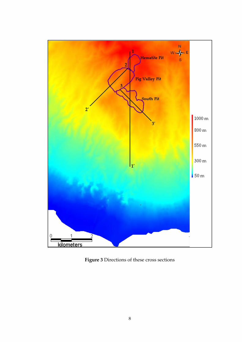
planned pit bottoms, cross sections were drawn; Figure 3 displays directions

of these cross sections. It should be noted that the topography displayed in

these cross sections is the initial topography before any excavation. In Figure

4; Cross Section 1-1’, passing through all pits, is shown. After Hematite Pit is

mined out in 3 years, it will be backfilled using some of the waste rock from

Pig Valley Pit.

8

Figure 3 Directions of these cross sections

9

Figure 4 Cross Section 1-1’ passing through all pits

Pig Valley Pit has a total surface area of 952,637 m² and the total mineable

reserve in this pit is 19.07 million tons. First stage of this pit is planned to

start operation in the 2nd year and the completion of all three stages is

planned to be achieved in the 12th year. In the Pig Valley Pit, the maximum

water level is around 783 m with minimum pit bench elevation of 500 m; in

this pit maximum required drawdown is 283 m. In Figure 5, Cross Section 2-

2’ passing through Pig Valley Pit is shown. The completed stages of Pig

Valley Pit will be backfilled with waste rock from its ongoing stages and

from South Pit.

10

Figure 5 Cross Section 2-2’ passing through Pig Valley Pit

The total surface area of the South Pit is 730,229 m² and the total mineable

reserve is 9.72 million tons. Within the 6th year, initiation of production in the

first stage of South Pit is planned and the completion is expected in the 15th

year (end of mine life). The maximum water level in this pit is 649 m;

minimum pit bench elevation producing the maximum required drawdown

is 440 m. In Figure 6, Cross Section 3-3’ which passes through South Pit is

shown. During the progress of South Pit, completed stages will be backfilled

with material from later stages being excavated.

11

Figure 6 Cross Section 3-3’ passing through South Pit

Surface area of the waste rock storage area is 1058.8 m². Here, the portion of

waste rock which is not used in backfill of pits will be dumped. Finally, the

surface area of the leach pad, where the crushed ore will be heaped and

leached with acid, is 1533.2 m².

1.4 Previous Works

1.4.1 Previous Works Within and Around the Study Area

Since 20th century, various geological studies have been carried out within

and around the Gediz Basin. Below, some of these studies are summarized.

12

The first geological study of the area dates back to 1915. In this study,

Philippson determined the age of the micaschist, clayey greywacke, gabbro,

diabase and limestone units as Paleozoic. In the following years, number of

studies increased rapidly. 1/500,000, 1/100,000 and 1/25,000 scale geological

maps of different parts of the region were prepared by the General

Directorate of Mineral Research and Exploration (MTA). Related with the

geology of the Gediz region, Bozkurt and Satır (2000); Yılmaz et al. (2000);

Bozkurt and Sözbilir (2004); Bozkurt and Rojay (2005); Yanık et al. (2006);

Çiftçi and Bozkurt (2009); and Thorne et al. (2009) carried out the most recent

studies. Furthermore, there are many studies about the geothermal areas in

the region.

District Office of State Hydraulic Works (DSİ) accomplished the earliest

hydrogeological investigation in the area in 1983; namely The

Hydrogeological Investigation Report for Gediz River Basin (Sarıgöl-

Alaşehir, Salihli-Turgutlu and Akhisar-Manisa Plains). Rather than the whole

surrounding region, more specific hydrogeological studies about Turgutlu

region were performed by Bank of Provinces (İller Bankası) but they focus on

the localities around the municipalities. In 2006, Turkish Environmental

Consulting Company, ENCON conducted environmental baseline studies

and completed the Environmental Impact Assessment (EIA) process in

Çaldağ Mine Site. The most recent hydrogeological study in Çaldağ area was

carried out by Yazıcıgil in 2008. In this area, any study regarding dewatering

requirement of the mine was not carried out.

13

1.4.2 Previous Works about Dewatering Simulations

Mine dewatering was crucial for the miners even in Neolithic times, where

no dewatering techniques were available, the mine had to be closed down

(Shepherd, 1993). The search for gold, silver, copper, iron and precious

stones sent people burrowing into the earth and thus into direct conflict with

groundwater. With the dawn of the Industrial Revolution by the 18th century,

the demand for coal was justifying all efforts to reach it. The British coal

mines pushed deeper more difficult water conditions. Endless rope

conveyors powered by horses on treadmills removed water in buckets.

Starting with 1770s, first early steam engines were used in mine dewatering.

It would be decades before wells with submersible electric pumps would be

used. The submersible electric motor developed for military use in Russia in

1915 was used in dewatering of Berlin subway in the 1920s. Today, with

appropriate regard to both theory and practice, effective dewatering can be

accomplished under almost any field conditions (Wolkersdorfer, 2008).

Mine development often causes penetration of water table and results in

groundwater flow into the mine. Dry working environments are preferred,

as they maintain efficient mining conditions; improve slope stability and

therefore safety (Van Mekerk, 1993).

The groundwater inflow to a mining excavation can be estimated using one

of these techniques: equivalent well approach, two-dimensional flow

equations or numerical techniques (Finite Difference Method, Finite Element

Method, and Boundary Element Method). Equivalent well approach assumes

that dewatering is achieved by use of an imaginary pumping well which

fully penetrates the entire saturated thickness of the aquifer. From this

14

borehole, water is pumped out at a uniform discharge rate in order to lower

the water level below the mining horizon at the mine boundary. Normally,

the mine excavation is seen as a large diameter deep well. When a surface

mine excavates below water table, groundwater flow into the excavation is

inevitable and this flow regime is essentially two dimensional. Remote from

the excavation, flow is linear but near the excavation there is vertical

component of flow and it is non-linear. Thus, the result of equivalent well

approach is very approximate. The two dimensional approach provides a

factor of safety by estimating inflows to be slightly higher than the

equivalent well approach and is a simpler tool (Singh and Reed, 1988). On

the other hand, the differential equations that describe the physical

phenomena can be solved analytically for limited class of problems and for

their simple geometries. As indicated on the University of Stuttgart, Institute

of Applied and Experimental Mechanics’ Web site (http://www.iam.uni-

stuttgart.de/bem/home_bem_introduc.html), more complex tasks require

numerical approaches. They provide powerful predictive tools able to model

a number of scenarios effectively. The application of finite difference, finite

element and boundary element techniques in dewatering problems predict

the quantities of inflow, clarify the pattern of water movement and identify

regions where flow rates are particularly large (Singh and Reed, 1988).

In this study, the flow rate to be used in dewatering was determined by

numerical modeling via modular finite difference groundwater flow model,

MODFLOW (Harbaugh et al., 2000). The following paragraphs of this

chapter assemble some of the studies in literature about determination of

dewatering rates in mining, via different modeling software.

15

Hydrogeological assessment of the planned underground gold mining in

Maud Creek Area, Northern Australia was carried out by Farrington and

MacHunter (2007) . In the area, a previously mined open cut with a length of

200 m, width of 100 m and depth of 26 m, is located and it is estimated to

contain 3x106 litres of water. After ten years of mining, the underground

mine is expected to be 700 m deep. Since groundwater levels in the area are

one to six meters below ground surface depending on topography, the pit

will be dewatered prior to mining and during development. For calculation

of groundwater inflows to the pit, groundwater modeling via MODFLOW

with SURFACT was accomplished. Reflecting the monthly mine schedule,

drain cells were used to obtain the amount of water to be abstracted and their

distribution coincides with the extent of mineralization. The dewatering rate

for the first year of mining was calculated to be 39.4 L/s and this rate

progressively decreased to 19.7 L/s after ten years of mining.

In the feasibility study conducted for Galore Creek copper-gold-silver project

in British Columbia, a numerical model was set up for open pit dewatering

simulation (Bruce, 2006). In this study; with the aim of evaluating pit inflow

rates and potential dewatering options, MODFLOW with SURFACT add-on

was used. According to the author, SURFACT adds the capability of

simulating variably-saturated flow to MODFLOW. In a model area of 300

km2 four open pits are located and the mine life is projected to be 20 years.

For the area to be dewatered; combination of vertical diameter wells, vertical

in-pit wells and horizontal drains is planned. Operational open pit mining

was input into the model by drains, which were activated to represent each

year of mining. According to the model, the groundwater inflow rate, when

there is no active dewatering, is approximately 27,000 m3/day (312.5 L/s).

16

Furthermore, a second numerical model was constructed via FEFLOW in

order to investigate the spacing of required horizontal drains (Bruce, 2006).

For the Diavik Diamond Mines located in the Canadian Shield, a numerical

groundwater flow model was constructed by Kuchling et al. (2000) to predict

groundwater inflow volumes and water quality with time. With this aim,

MODFLOW and MT3DMS were used. Initial mine plan constitutes three

open pit mines and underground mining which will continue afterwards,

underneath two of the open pits. The timely changes in pit extents were

integrated into the model by automatically adjusting the model boundaries

every two years throughout the twenty year mine life. In this study, results

of modeling indicated that the total mine inflows are expected to reach a

maximum value of 9600 m3/day (111.1 L/s) and TDS concentrations gradually

increase in time to a maximum about 440 mg/L.

In 2001, Williamson and Vogwill constructed a three-dimensional

groundwater model to predict the dewatering requirements associated with

open-pit mining in the Lihir Gold Mine, New Guinea. The ore bodies in the

area are located in a collapsed volcanic crater in an active geothermal field

adjacent to sea, and for safe and efficient mining conditions together with pit

wall stability, dewatering was required. It is important to note that when this

study was carried out there was ongoing mining and dewatering operations

in the field; this study had the aim of solving previously faced problems in

dewatering. The constructed model included density and viscosity coupling

to allow geothermal heat effects on groundwater flow to be simulated, and it

was run in conjunction with a geothermal model. For a total drawdown of

200 m, the total required pumping rate was calculated to be 1000 L/s. In this

17

study, the final dewatering schedule in the mine area constitutes 8

dewatering bores with average depth of 275 m (pumping rate of each

ranging from 50 to 130 L/s) and over 100 horizontal drainholes up to 200 m

long (with rates up to 5 L/s).

18

CHAPTER 2

DESCRIPTION OF THE STUDY AREA

2.1 Morphology

The study area is located within the Aegean Region. It is characterized by

steep and undulating topography, with an altitude ranging from 50 m above

sea level in the south, to 1034 m at Ayşekızı Hill in the north. Hills with

significant elevations in the study area include Akyatak Hill (960 m),

Sırayatak Hill (790 m), Sakar Hill (625 m) and Taşgöl Hill (590 m).

Considering the hills in the area as check points, Digital Elevation Model

(DEM) enclosing the study area was modified from Ağartan (2010). It was

created from a 1/25,000 scaled topographic map with 12.5 m grid size using

MapInfo 8.5 Software (Figure 7).

19

Figure 7 Digital Elevation Model (DEM) of the model area

2.2 Climate and Meteorology

Conformable with the climatic conditions of Aegean Region in which the

area is located; the climate is mild with soft springs, hot and dry summers,

sunny autumns and warm winters with occasional showers. Due to the

character of Aegean Region with mountains perpendicular to the shores, sea

20

climate (similar to Mediterranean climate) reaches inner parts of the region

where continental climate is more dominant. Thus, the study area is

characterized by a typical Mediterranean climate with relatively high

average annual temperatures. Due to high altitudes in northern parts,

temperatures slightly cooler than the rest of the region are experienced with

some snow and frost days.

Around the area; six meteorological stations, established by the State

Meteorological Organization (DMI), are present at Manisa, Akhisar, Salihli,

Saruhanlı, Gölmarmara and Turgutlu (Figure 8). Manisa, Akhisar and Salihli

stations are principal meteorological stations which measure hourly

temperature, solar radiation, wind speed and direction, three times daily

precipitation and monthly maximum precipitation. Saruhanlı, Gölmarmara

and Turgutlu are ordinary meteorological stations which measure

temperature, wind speed and direction, and precipitation (three times daily

and daily total). Detailed information about meteorological stations is given

in Table 1.

21

Figure 8 Meteorological stations around the study area (Modified from

(Yazıcıgil, 2008).

Table 1 Detailed information about meteorological stations

Station

Number

X-

Coordinate

Y-

Coordinate

Period of Data

Availability

Elevation

(m)

Saruhanlı 5269 549301 4287516 1986-1995 -

Gölmarmara 5273 579741 4285913 1984-1991 -

Turgutlu 5615 561087 4261704 1984-2006 120.000

Akhisar 17184 570865 4306176 1937-2006 92.034

Manisa 17186 537773 4274507 1930-2006 71.000

Salihli 17792 598897 4260231 1939-2006 111.000

22

2.2.1 Temperature

The average annual temperature in the region is 16.34°C. January and

February are the coldest months with average monthly minimum

temperature of -4.44 °C; while July is the hottest month with average

monthly maximum temperature of 39.76 °C. In Table 2; average monthly

minimum and maximum temperature values together with monthly

minimum and maximum observed ones are given for the regional network.

23

Table 2 Monthly minimum and maximum observed, average monthly

minimum and maximum temperature values for the regional network

Saruhanlı Gölmarmara Turgutlu Akhisar Manisa Salihli

Min.

Monthly

Temp. °C

-8.2 -7.8 -10 -13.2 -13.1 -13.5

Month &

Year

of

Observation

Feb

1992

Feb

1985

Feb

2004

Jan

1954

Jan

1954

Feb

2004

Max.

Monthly

Temp. °C

42 43.2 44.9 44.6 45.1 44.8

Month &

Year

of Obs.

Jul

1987

Jul

1987

Jul

2000

Aug

1958

Jul

2000

Jul

2000

Ave. Min.

Monthly

Temp. °C

-5.13 -4.06 -3.81 -5.25 -4 -4.4

Month of

Obs. Feb Feb Jan Jan Jan Jan

Ave. Max.

Monthly

Temp. °C

39.76 39.6 39.93 39.83 40.02 39.42

Month of

Obs. Jul Jul Jul Jul Jul Jul

Ave Temp.

°C 15.9 16.3 16.7 16.1 16.9 16.3

24

2.2.2 Relative Humidity

The average relative humidity for all State Meteorological Organization

(DMI) stations varies from about 46% in June and July, to 75 % in December,

with a yearly average of 60% (Table 3). Among the stations in the region,

Akhisar has the highest humidity whereas Gölmarmara has the lowest. The

average monthly relative humidity for each station is displayed in Figure 9.

25

Table 3 Average monthly relative humidity for stations

Saruhanlı Gölmarmara Turgutlu Akhisar Manisa Salihli

Min. Monthly

Relative

Humidity (%)

36.8 34.1 33 37.8 35.5 39.8

Month & Year

of

Observation

Jul

1994

Jul

1985

Jun

2001

Jun

2003

Jul

1945

Jun

2001

Max. Monthly

Relative

Humidity (%)

83.2 76.2 82.5 86.3 88.2 86.3

Month & Year

of

Obs.

Dec

1990

Dec

1985

Dec

2004 Dec 1950

Dec

1950

Jan

1982

Average Min.

Relative

Humidity (%)

44 38.46 47.99 50.49 44.55 50.22

Month of

Obs. Jul Jun Jul Jul Jul Jun

Ave. Max.

Relative

Humidity (%)

76.06 71.7 76.84 76.84 76.22 75.17

Month of

Obs. Dec Dec Dec Dec Dec Dec

Ave.Relative

Humidity (%) 58.5 53.4 61.5 63.9 60.9 62.7

26

Figure 9 Average monthly relative humidity graph for each station

2.2.3 Precipitation

The distribution of average monthly precipitation for the stations in the

regional network is shown in Figure 10. December is the wettest month for

each station, and except Gölmarmara station, August is the driest month. The

dry summer period extends from June through to early September, and the

wet winter period extends from November to February.

27

Figure 10 Distribution of average monthly precipitation for the stations in the

regional network

On an annual basis, data show that Manisa is the station that receives most

precipitation (736 mm/year), while Saruhanlı (445 mm/year) and

Gölmarmara (447 mm/year) receive the least. This is probably due to the

availability of a longer period of record (1943-2006) at Manisa station which

includes a series of wet and dry years, giving a representative average

annual value. The same is also true for Salihli (1939-2006) and Akhisar

stations (1943-2006) where long term data is available. The short term data

collected at Saruhanlı (1986-1995) and Gölmarmara (1984-1991) correspond to

a long-term dry period that was present in the region from 1982 to 1996.

28

2.2.4 Evaporation

In the region, evaporation is only monitored at Akhisar and Salihli stations.

The monitoring is usually carried out from April to November. Hence there

were missing data belonging to the months with low evaporation. These

missing data were calculated by correlation between measured monthly

evaporation and average monthly temperature data, where available. The

average monthly evaporation values at Salihli and Akhisar stations are

plotted in Figure 11. In July and January, the average monthly maximum and

minimum evaporations were observed, respectively. In addition, the yearly

average evaporation was calculated as 1377 mm (Yazıcıgil, 2008).

Figure 11 Average monthly evaporation at Salihli and Akhisar stations

29

2.2.5 Wind

Monthly wind speed data for Akhisar, Manisa and Salihli stations indicate

that the average annual wind speeds range between 1.0 m/s and 3.0 m/s. In

July and August, generally the highest wind speeds are observed (Figure 12).

Figure 12 Average monthly wind speed

30

2.3 Geology

2.3.1 Regional Geology

Western Turkey is known to be the site of widespread active N-S continental

extension. Forming the eastern part of Aegean extensional province, the

region is currently under the influence of forces resulting from convergence

of African and Eurasian plates. The region has been subjected to this N-S

extension since, at least, latest Oligocene-Early Miocene. The outstanding

structures of the area are; E-W trending grabens and intervening horsts,

exposing the Menderes Massif (Bozkurt and Sözbilir, 2004). The Menderes

Massif is one of the two large metamorphic culminations within the Alpine

Orogen of Turkey, the other one being the Kırşehir Massif (Bozkurt and Satir,

2000). It is geographically divided into three sub-massifs along E-W trending

Gediz and Büyük Menderes Grabens (Figure 13), as northern, central and

southern (Bozkurt and Rojay, 2005).

31

Figure 13 Outline geological map of western Anatolia showing Neogene and

Quaternary basins and subdivision of the Menderes Massif. The sequences of

Miocene and Pliocene age are not differentiated. BH- Bozdağ horst, AH-

Aydın Horst, CMM- Central Menderes Massif, NMM- Northern Menderes

Massif, SMM- Southern Menderes Massif, Ak- Akhisar, Gö- Gördes, De-

Demirci, Se- Selendi, Kz- Kiraz, Gk- Gökova, Sö- Söke. (Modified from

Bozkurt and Rojay, 2005)

The area focused in this study (Çaldağ Region) is located on the northern

edge of Menderes Massif, on a horst block to the north of Gediz Graben

(Thorne, et al., 2009). Gediz Graben starts southeast of Alaşehir to the east

32

and extends westward for more than 100 km to Turgutlu and beyond, along

the plain of Gediz River. It is probably the best developed graben in Turkey,

regarding the accumulated sediment thickness and total offset along the

graben-boundary structures (Çiftçi and Bozkurt, 2009). The E-W trending

graben is asymmetric with steeper and seismically more active southern

margin (Yilmaz et al., 2000).

The rock units exposing in the vicinity of Gediz Graben can simply be

grouped into two, as basement and cover units. Metamorphic rocks of the

Menderes Massif constitute the pre-Neogene basement. Above them; cover

units of ages varying from Miocene to Recent, lie unconformably (Çiftçi and

Bozkurt, 2009).

2.3.2 Site Geology

Çaldağ occurs as an isolated mountain sequence consisting of various

geological units surrounded by a plain of young sediments. From oldest to

youngest, the rock units cropping out in the study area include: rocks

belonging to the İzmir-Ankara Suture Zone (Brinkman, 1966), laterites

formed over the ultrabasic rocks of this zone, Kanlıtepe Formation consisting

of lacustrine and fluvial sediments (Yanık et al., 2006) and alluvium

unconformably overlying all these units (Figure 14).

33

Figure 14 Geological map of the study area (Modified from (Yazıcıgil, 2008)

using MTA map)

İzmir-Ankara Suture Zone rocks are Late Cretaceous-Paleocene aged, and

are part of an accretional prism consisting of ultrabasic, serpentinized

ultrabasic and spilitic volcanic rocks with pelagic matrix. The matrix consists

of sandstone, mudstone, claystone, limestone, radiolarite and chert. Triassic

aged, neritic, dolomitic limestone blocks occur as olistoliths in this matrix.

Low grade metamorphism, probably related to tectonics during the closure

34

of the ocean, can be seen in the lower levels of the accretional prism

(Yazıcıgil, 2008).

Neogene units cover all of the sequence with an unconformity. They are

represented by two groups; Miocene rocks and Pliocene rocks (Ağartan,

2010). The Miocene rocks in the study area are laterites. The Late Cretaceous

aged serpentinized ultrabasic rocks were influenced by tropical-subtropical

climatic conditions which dominated the western Anatolia during Miocene,

leading to the formation of laterites. Consequently; these rocks were exposed

to extreme physical and chemical weathering. This way, relatively mobile

elements like Ni, Co, and Mn were leached and re-deposited at depths in the

profile, while stable elements such as Fe and Al concentrated in the upper

part of the profile, in the form of oxides and hydrated oxides. They formed a

duricrust protecting the laterite from erosion.

Pliocene rocks in the area are represented with mostly detritic, lacustrine and

fluvial sediments; named as Kanlıtepe Formation. There is an angular

unconformity between the Kanlıtepe Formation and the underlying older

rock units. Sediments are preserved as patches due to physical weathering.

Alluvium is seen at low lands in south of the study area and occupies the

entire plain of Gediz River. This Quaternary alluvium consists of clay, silt,

sand and gravels and unconformably overlies the older units (Yazıcıgil,

2008).

35

CHAPTER 3

HYDROGEOLOGY

3.1 Water Resources

The study area is located within the central part of the Gediz River’s 17,118

km2 catchment area. Gediz River forms the southern boundary of the model

area and flows towards west to the Aegean coast, discharging through the

Gediz Delta in the outer part of İzmir Bay. In the study area no surface water

reservoir or lake is located; Gölmarmara Lake lies about 19 km and

Demirköprü Dam is about 50 km east of the area.

3.1.1 Surface Water Resources

Gediz River, forming the southern boundary of the study area, is the major

water resource within the study area. It flows in an E-W direction, and

receives discharge from numerous creeks. Drainage pattern and major

surface waters of the area are displayed in Figure 15.

36

Figure 15 Drainage patterns, major surface waters, surface water monitoring

stations and streamflow gauging stations in the region

Streamflow gauging stations:

37

In the study area, there are 13 surface water monitoring stations established

by the company owning the operating licence of the mine. The locations of

these monitoring stations together with the drainage pattern are also given in

Figure 15. Due to the short observation period and lack of data, Soil

Conservation Service (SCS) curve number method was used in the

calculation of runoff from the project area sub-watersheds. Soil Conservation

Service (1964) runoff estimates assume a relationship between accumulated

total storm rainfall P, runoff Q, and infiltration plus initial abstraction (F+Ia).

It is assumed that F/S=Q/P. Where F is infiltration after the beginning of

runoff, S is potential abstraction, Q is direct runoff in inches, and Pe is

effective storm runoff (P-Ia). With F = (Pe-Q) and Pe = (P-Ia) = (P-0.2S); based

on data from small watersheds, Q = (P-0.2S)2/(P+0.8S).

The SCS method uses the runoff curve number CN, related to potential

abstraction by CN = 1000/(S+10), S being in inches. Thus, runoff curve

numbers (CNs) indicate the runoff potential from a hydrologic soil-cover

complex during periods when the soil is not frozen. A higher CN indicates a

higher runoff potential. Runoff curve numbers vary as a function of land use,

cover, and hydrologic soil groups. Hydrologic soil groups are divided into

four types: A, B, C, and D. Hydrologic soil group A is sandy and well

drained, group B is sandy loam, group C is clay loam or shallow sandy loam,

and group D is heavy plastic clay that swells when wet. Group D is a poorly

drained soil. Using satellite image and forestry maps with hydrologic soil

group C, a weighted CN is calculated for each sub-watershed based upon the

percent of area covered by various types of covers. The calculated CNs for

sub-watersheds varied from a minimum of 75.1 to a maximum of 82.3 as

38

displayed in Table 4. The weighted CN value for the study area is 77

(Yazıcıgil, 2008).

Table 4 Runoff curve number calculation

Several streamflow gauging stations were established on the Gediz River and

its tributaries by the State Hydraulic Works (DSİ) and Electrical Power

39

Resources Survey and Development Administration (EİEİ). Stations 518 and

533 are located downstream and upstream of the study area, respectively;

and have been recording data for long periods (Figure 15). The streamflow

gauging station 518 has been recording flow rates for approximately 40

years, while station 533 has been recording for 13 years.

The monthly river flow rates show the effect of winter rainfall and the

controlled releases of discharges from Demirköprü Dam and the

Gölmarmara Lake. The flow rates are higher in the winter and early spring

(January through March) following the high amount of winter rainfall and

then decrease through spring and early summer. It is natural that the flow

rates are low in summer and fall months; however with the release of water

from Demirköprü Dam and the Gölmarmara Lake, the rates are kept at a

moderate level. Thus, as a result of DSI’s control, the lowest river flows

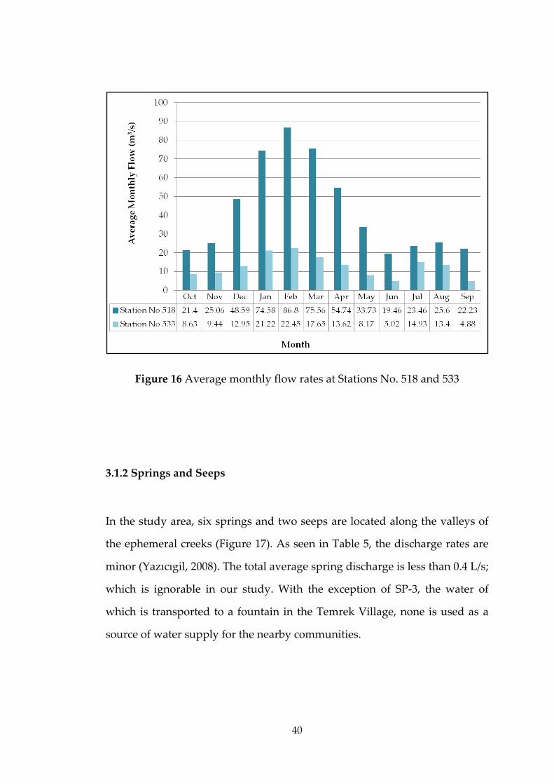
typically occur in May-June and September-October. Hence, the average

monthly discharge at Station 518 varies from a maximum value of 86.8 m3/s

in February to a minimum value of 19.46 m3/s in June; the average annual

being equal to 42.5 m3/s. The average monthly discharge at Station 533 varies

from a maximum value of 22,45 m3/s in February to a minimum value of 4.88

m3/s in September; the average annual being equal to 12.7 m3/s (Yazıcıgil,

2008). Related graph about average monthly flow is displayed in Figure 16.

40

Figure 16 Average monthly flow rates at Stations No. 518 and 533

3.1.2 Springs and Seeps

In the study area, six springs and two seeps are located along the valleys of

the ephemeral creeks (Figure 17). As seen in Table 5, the discharge rates are

minor (Yazıcıgil, 2008). The total average spring discharge is less than 0.4 L/s;

which is ignorable in our study. With the exception of SP-3, the water of

which is transported to a fountain in the Temrek Village, none is used as a

source of water supply for the nearby communities.

41

Figure 17 Springs and seeps in the study area

42

Table 5 Discharge rates of springs

Spring

Coordinates

Elevation

(m)

Unit

Average

Discharge

(L/s)

Easting Northing

SP-1 567442 4275846 946 Kanlıtepe Formation 0.14

SP-2 566205 4275293 665 Ultramafic Rocks 0.05

SP-3 565967 4275072 609 Ophiolitic Melange 0.05

SP-6 565451 4275066 395 Ultramafic Rocks 0.06

SP-7 565620 4269434 90 Kanlıtepe Formation 0.02

SP-8 567490 4274105 715 Ultramafic Rocks 0.02

3.1.3 Wells

In the study area; there are 184 wells, all of which are drilled by individuals.

All the wells located in the area are used for irrigational purposes (Figure 18).

43

Figure 18 Wells located in the area

44

3.2 Groundwater Bearing Units

3.2.1 Hydrogeologic Classification of Groundwater Bearing Units

The principal aquifer of regional importance in the vicinity of study area is

the Quaternary alluvium aquifer that occupies the plain areas along the

Gediz River to the south of the area. It consists of a mixture of clay, silt, sand,

gravel and boulders. The underlying sandstones, conglomerates and the

limestones of the Kanlıtepe Formation also form a regional aquifer of

secondary importance (Figure 19). These deposits are thickest in the central

part of the valley, in the region of the Gediz River, and thin to the edges of

the valley where they abut against the older rocks. Some of the project area

and its vicinity are underlain by these Neogene age sedimentary deposits.

The laterites and ultrabasic rocks belonging to the İzmir-Ankara Suture Zone

have low permeability to render them as aquifers. The fractured sections of

these formations may locally form perched aquifers to yield water to some

ephemeral springs.

45

Figure 19 Hydrogeological map of the study area

3.2.2 Hydraulic Properties of Groundwater Bearing Units

There are 11 groundwater monitoring wells (GK-1 to GK-11) within the

study area (Figure 19). Hydraulic conductivity and storativity values were

obtained regarding the results of pumping tests conducted at these wells. In

Table 6, detailed information about monitoring wells is given. Although

46

initially four wells were targeted in laterites, only one (GK-1) could be tested

because GK-3, GK-4, and GK-5 were dry. The laterites in GK-1 has the

highest hydraulic conductivity tested (2.89 x 10-6 m/s). The fault extending

through the Pig Valley probably passes through the Hematite Pit and GK-1

and contributes to a relatively higher permeability by fracturing the rock

units around GK-1. The hydraulic conductivity of ultramafic rocks were

tested at two (GK-2 and GK-6) monitoring wells, both giving almost the same

magnitude of hydraulic conductivity value of about 6.5x10-7 m/s. The

hydraulic conductivity of Kanlıtepe formation, tested in four (GK-6, 7, 8, 9,

and 11) wells varies from 1.16x10-8 m/s to 1.23x10-6 m/s, the geometric

average being equal to 1.37x10-7 m/s. The variation in hydraulic conductivity

of the Kanlıtepe formation is several orders of magnitude, indicating the

highly heterogeneous nature of the formation. Table 7 summarizes the

hydraulic parameters calculated from pumping tests. In the study area, there

are no monitoring wells drilled into the alluvium; thus for the hydraulic

conductivity of alluvium, data from a study of the whole Gediz River Basin

was used (Ağartan, 2010). Consequently, hydraulic conductivity of alluvium

is 4.6x10-5 m/s.

47

Table 6 Information about monitoring wells

Well

Name

Easting

(m)

Northing

(m)

Ground

Elevation

(m)

Borehole

Depth

(m)

Depth to

Water

(m)

Target

Formation

GK-01 567470 4276017 956.23 100 57.03 Laterite

GK-02 567143 4275220 820.84 62.5 19.68 Ultramafic

Rocks

GK-03 566700 4273940 615.02 85 - Laterite

GK-04 567269.5 4273507 558.37 81 - Laterite

GK-05 567571 4273103 583.38 140 - Laterite

GK-06 565235.3 4274199 390.36 75 Artesian Ultramafic

Rocks

GK-07 565298.6 4273260 358.48 207 76.15 Kanlıtepe

Formation

GK-08 564917 4272951 284.65 86 27.33 Kanlıtepe

Formation

GK-09 564825 4271561 178.28 90 28.76 Kanlıtepe

Formation

GK-10 565613 4270882 188.75 84 47.51 Kanlıtepe

Formation

GK-11 565925.6 4268971 85.39 112 40.6 Kanlıtepe

Formation

48

Table 7 Summary of hydraulic conductivity and storativity parameters

Hydraulic Conductivity (m/s) Storativity

K

(min)

K

(max)

K

(Arithmetic

Average)

K

(Geometric

Average)

S

(min)

S

(max)

Laterite - - 2.89E-06 - 0.148

Ultramafic 5.58E-07 7.43E-07 6.50E-07 - 0.033

Kanlıtepe

Formation 1.16E-08 1.23E-06 4.63E-07 1.37E-07 0.01 0.22

The calculated storativities are generally low (0.02), except at GK-1 and GK-9

where they are high (0.15-0.22). The higher values noted at these wells may

have been produced by the fracturing and faulting that affects them. Both of

them are located on probable faults.

3.2.3 Groundwater Levels

3.2.3.1 Spatial Variation in Groundwater Levels

Using spring elevation data and available groundwater level data from

monitoring wells, a groundwater elevation map was developed. The

elevations of the springs located in the western part of the project area (SP-2,

SP-3, SP-5 and SP-6) were conformable with the regional groundwater levels;

however elevations of the springs located in the north and east of the area

49

(SP-1, SP-4 and SP-8) were significantly above the regional water table

contours. Hence, these three springs are probably discharging from a local

perched aquifer.

Groundwater flow in the study area is from N-NE toward S-SW as shown in

the groundwater level map in Figure 20. Groundwater levels decrease from

about 900 m in the north to 50 m in the south along the Gediz River. Thus,

the northern boundary where Çaldağ is located forms a recharge boundary.

The Gediz River located in the south, forms a drainage boundary where most

of the discharge takes place. The hydraulic gradient is relatively higher

(about 0.2) in the northern part of the area where laterites and ultramafic

rocks crop out and it is lower (0.10 to 0.06) at the southern part of the area

where Kanlıtepe Formation crops out. Lower gradients at the southern part

correspond to the relatively thicker and permeable Kanlıtepe Formation

(Yazıcıgil, 2008). Additionally, depth to water table map is given in Figure 21.

The evaluation of groundwater levels indicate that the deeper parts of the

planned pits will encounter a standing water level which have to be lowered

by dewatering to permit dry working conditions. In Part 1.3, Figures 4, 5 and

6; this was explained in more detail.

50

Figure 20 Groundwater level map of the study area

51

Figure 21 Map of depth to water table

3.2.3.2 Temporal Changes in Groundwater Levels

In the groundwater monitoring wells mentioned in Part 3.2.2, water levels

are measured since 2008. The most recent measurement is 14.09.2011 dated.

The target formations of these wells (as previously displayed in Table 6) are

laterite for GK-1, ultramafic units for GK-2 and 6, and Kanlıtepe Formation

for GK-7, 8, 9, 10 and 1in Part 3.2.2 displays the locations of these wells.

52

Figure 22Figures 22, 23, 24, 25, 26, 27 and 28 display the temporal water level

changes in monitoring wells. Examination of Figure 22 and 23 together,

shows that the rise in water levels corresponds to February and decrease

starts in June and May in GK-1 and GK-2, respectively. It can be concluded

that GK-1 and GK-2, which are the northernmost located monitoring wells in

the area, display seasonal fluctuations. In other wells, these fluctuations are

not observed. The maximum change in the groundwater levels, which is 9.5

m, is observed in GK-2.

Figure 22 Temporal water level changes in monitoring well GK-1

53

Figure 23 Temporal water level changes in monitoring well GK-2

Figure 24 Temporal water level changes in monitoring well GK-7

54

Figure 25 Temporal water level changes in monitoring well GK-8

Figure 26 Temporal water level changes in monitoring well GK-9

55

Figure 27 Temporal water level changes in monitoring well GK-10

Figure 28 Temporal water level changes in monitoring well GK-11

56

3.2.4 Water Balance and Groundwater Recharge

As mentioned before; using SCS curve number method, runoff was

calculated as 140.4 mm/yr. In order to calculate potential evapotranspiration,

Thornthwaite method was used. In the water balance equations, the long-

term average monthly temperature and average monthly precipitation

values for Turgutlu meteorological station were used. Initial soil moisture

value is assumed as 100 mm. The results of water balance calculations are

summarized in Table 8. The results show that, 61.4% of the annual

precipitation is lost into the atmosphere as actual evapotranspiration, 27.8 %

runs off, and 10.8 % percolates into the ground to recharge the groundwater

system.

Table 8 Annual Water Balance Results for the Project Area

Annual Amount

(mm)

Proportion of Annual

Rainfall (%)

Precipitation 505.3 100

Evapotranspiration 310.3 61.4

Runoff 140.4 27.8

Percolation 54.6 10.8

57

CHAPTER 4

GROUNDWATER FLOW MODEL

4.1 Software Description

Modular finite difference groundwater flow model, MODFLOW-2000 code

developed by the United States Geological Survey (USGS) was used in this

study (Harbaugh et al., 2000). The groundwater model in the study was

developed using Visual MODFLOW 2010.1, which is a graphical interface for

MODFLOW. In Visual MODFLOW; MODFLOW, MODFLOW-SURFACT,

MT3DMS, SEAWAT and ZONEBUDGET can be integrated.

Since 1980s, MODFLOW is continuously being developed with new

packages and tools. Worldwide, it is widely used in groundwater flow

modeling. Selection of this software in this study was based on these

specifications:

- It can simulate regional models, and visualize the results using 2D or 3D

graphics,

- It is capable of simulating a wide variety of hydrogeologic processes in field

conditions and various geological features,

- It can simulate confined, unconfined and leaky aquifers under both steady-

state and transient conditions.

58

4.2 Conceptual Model

As explained in part 3.2.1, main aquifer of regional importance is the

alluvium aquifer that occupies the plain areas in the south. The underlying

Kanlıtepe Formation also forms a regional aquifer of secondary importance.

The laterites and ultrabasic rocks of İzmir-Ankara Suture Zone have low

permeability to render them as aquifers but fractured sections of these

formations have high hydraulic conductivity. Conceptual model

development is the main step of modeling, thus detailed examination of the

system is necessary. Since the model area is complex and rapid changes in

elevation occur in short distances, it is important to simulate the

heterogeneity in detail, both by horizontal and vertical means. This is

achieved by means of fine grid cell sizes and large number of layers.

Considering the main purpose of the study, which is the determination of

dewatering requirements for the mine, the deepest pit bottom elevations

were evaluated for the thickness of first layer. Bottom of the first layer is

assigned to be below the deepest pit bottom elevation. The underlying three

layers have varying thicknesses and the bottom lowermost layer is at -600 m.

Figure 29 is a N-S directional cross section showing the modeled layers.

59

Figure 29 N-S cross section displaying four model layers

In the conceptual model, the first layer is composed of four different units

depending on different hydraulic conductivities: Alluvium, Kanlıtepe

Formation, laterites and rocks belonging to İzmir-Ankara Suture Zone.

Downwards, each layer also constitutes four units. During calibration, this

grouping was changed and number of units in each layer increased.

4.3 Model Setup

4.3.1 Finite Difference Grid

Gridding is obligatory in order to define and discretize the domain. To be

able to obtain a reasonable solution time, the minimum number of grids that

will best display the boundaries and heterogeneity of the aquifer should be

60

selected. The grid size is selected to be 50 m in both rows and columns, and is

refined to 25 m (in both directions) in areas where the three open pits, leach

pad area and waste rock storage area are located. 25 m grid size was also

chosen for the area close to the northern model boundary since heads in this

area display abrupt changes in short distances and it is important to correctly

simulate this complexity. The gridded model domain is displayed in Figure

30.

61

Figure 30 Gridded model domain

62

4.3.2 Boundary Conditions

In the case of a groundwater flow model, boundary conditions describe the

exchange of flow between the model and the external system. Geological and

hydrogeological characteristics of the area are mainly considered in

determination of model boundaries. As mentioned and displayed before

(Figure 20), flow direction in the study area is from northeast to southwest.

Thus, to simulate the continuous inflow to the model domain from the

northern boundary, general head boundary condition was assigned to this

portion. Similarly; in order to simulate the outflow of water from the system

in the northwestern part, general head boundary condition was assigned to

this part as well. While assigning general head boundary condition, the

boundary head was obtained from topography corresponding to the selected

cells. Boundary distance was taken as 100 m and conductance was

automatically calculated by the software via default conductance formula.

Gediz River flows along the southern boundary of the model domain, so it

was simulated with river package. While assigning the river, river stage

elevation was assigned to be 5 m below the corresponding topography in

river cells, river bottom elevation to be 0.5 m below the stage and riverbed

thickness to be 1m. Using the input parameters, the software calculated the

conductance by default conductance formula.

Additionally, major creeks in the study area are modeled as drains. Drains

remove water from the system as long as the water table is above specified

drain elevation; otherwise, when the drain elevation is below water table, the

drains have no effect. The drain package in MODFLOW is the most relevant

63

one for simulating seasonal water flow in a creek (Duru, 2004). In the model;

the drain elevation was assigned to be 5 m below the topography and

initially, the conductance was assigned as 1000 m2/day for all the drains

representing the creeks, during calibration this parameter was changed too.

Finally, no flow boundary condition was used for the rest of the boundaries.

In Figure 31, boundary conditions are displayed.

Figure 31 Boundary conditions

64

4.3.3 Hydraulic Parameters

As explained in part 4.2, at model setup 16 different hydraulic conductivity

zones (4 zones for each of 4 layers) were defined. During calibration, number

of zones was changed together with hydraulic conductivity values. Initially;

in the first layer, the hydraulic conductivity values explained in part 4.2.2

were assigned. These are determined due to pumping tests. In second, third

and fourth layers, hydraulic conductivity zones have the same spatial

distributions but their numeric values are half of the upper one in each layer.

Figure 32 displays the initial hydraulic conductivity distribution of first layer

in plan-view. Also in Figure 33, the hydraulic conductivity zones assigned in

conceptual model are shown on N-S directional cross section.

65

Figure 32 Hydraulic conductivity distribution of first layer in plan view in

the conceptual model

66

Figure 33 Hydraulic conductivity zones in the conceptual model, N-S

directional cross section

4.3.4 Areal Recharge

Recharge from precipitation is the most important source for groundwater

recharge, and as mentioned previously in part 3.2.4, it was calculated using

Thornthwaite method. The calculated recharge value is 54.6 mm/yr but it

was not assigned uniformly to the whole region. In the northeastern part

where elevation is above 500 m; the recharge value was assigned to be 109.2

mm/yr (twice the calculated value). This is due to the fact that the elevation

rises up to 1034 m and even snow is observed in these elevated areas,

causing higher amounts of groundwater recharge than the rest of the region.

Figure 34 displays the recharge distribution in the study area.

67

Figure 34 Recharge distribution in the study area

4.3.5 Wells

According to the DSI reports, water requirement of the area to be irrigated by

wells was determined as 0.61 L/s/ha. It is assumed that pumping from the

wells for irrigation purposes occur only in June, July, August and September.

With the help of Google Earth, it was determined that the irrigation fields

have an area of 2371 ha, requiring 14.995 hm3 of water annually. After this

68

calculation, discharges of the 172 wells introduced to the model were

determined to be 238.86 m3 / day.

4.4 Model Calibration

4.4.1 RMS and Normalized RMS of the Calibrated Model

After the completion of model setup by introducing all the inputs to the

software, calibration was carried out. In order to match the calculated

groundwater levels with the observed ones; recharge, boundary conditions,

hydraulic parameters and drain conductance values were adjusted within

the limits of geology and hydrogeology.

One of the criteria in obtaining a satisfying match between calculated and

observed heads is acquiring the minimum possible RMS (Root Mean Squared

Error) or Normalized RMS. They are defined by Equations 1 and 2,

respectively.

(1)

(2)

In these equations,

n : total number of observation points,

hobs : observed groundwater level,

hcal : calculated groundwater level.

69

RMS is expressed in length units and Normalized RMS is expressed as

percentage. The latter is a more representative measure of the fit, as it

accounts for the scale of the potential range of data values. The

aforementioned two values were calculated for all the wells located in the

model area, and the calibration is achieved with a RMS of 39.194 m and a

Normalized RMS of 4.569 %. The calibration graph is displayed in Figure 35.

Considering the complexity of the region, this is a very successful fit; hence,

it can be concluded that a good match between observed and calculated

groundwater levels is obtained. Observed and calculated groundwater levels

at the end of calibration are displayed in Figure 36.

Figure 35 Calibration graph

70

Figure 36 Observed heads (a) and calculated groundwater levels (b)

The new hydraulic conductivity distribution in the first layer after calibration

can be seen in Figure 37. In the conceptual model, some units were grouped

(ultramafic units and limestones) and assigned same hydraulic conductivity

values. However, in the calibration step, regarding the comparison of

calculated and observed heads, they were separated. As explained before; in

layers 2, 3 and 4, hydraulic conductivities have same spatial distributions as

the ones in the first layer but going downwards, each zone has a value half of

the one above it.

71

Figure 37 Hydraulic conductivity distribution in Layer 1 after calibration

In order to obtain a satisfying match between observed and calculated heads,

boundary conditions were edited too. The general head boundary at the

northern border was edited via changing boundary head and boundary

distance values. Additionally, conductance values of the drains denoting the

72

seasonal creeks were modified. In the conceptual model, the drain

conductance value was assigned as 1000 m2/day uniformly; however during

calibration this value was increased to 3000 m2/day in some regions. In

regions where the calculated heads were significantly higher than the

observed ones and when change of hydraulic conductivity was not enough

for obtaining a good match, drain conductance was increased. With trial and

error, 3000 m2/day was found to be the most satisfying value.

4.4.2 Calculated Groundwater Budget

Using the calculated groundwater budget, it is possible to examine the

recharge and discharge mechanisms of the model domain. Depending on the

results of the steady-state model, components of the groundwater budget

calculated under equilibrium conditions were examined. The groundwater

budget calculated at the end of calibration for the whole domain is given in

Table 9. The model domain is recharged from precipitation (4.63 hm3/yr),

from flow along northern and northwestern boundaries (24.13 hm3/yr) and

from Gediz River (2.50 hm3/yr), which make a total recharge of 31.26 hm3/yr.

In the system, as expected there is balance between recharge and discharge.

Furthermore; 49.2 % (15.37 hm3/yr) of the total recharge is discharged

through wells, 32.5 % (10.17 hm3/yr) as subsurface outflow, 15.4 % (4.82

hm3/yr) from creeks, 1.6 % (0.50 hm3/yr) via evapotranspiration and 1.3 %

(0.40 hm3/yr) through Gediz River.

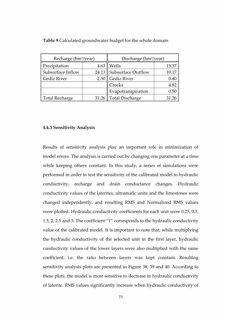
73

Table 9 Calculated groundwater budget for the whole domain

Recharge (hm3/year) Discharge (hm3/year)

Precipitation 4.63 Wells 15.37

Subsurface Inflow 24.13 Subsurface Outflow 10.17

Gediz River 2.50 Gediz River 0.40

Creeks 4.82

Evapotranspiration 0.50

Total Recharge 31.26 Total Discharge 31.26

4.4.3 Sensitivity Analysis

Results of sensitivity analysis play an important role in minimization of

model errors. The analysis is carried out by changing one parameter at a time

while keeping others constant. In this study, a series of simulations were

performed in order to test the sensitivity of the calibrated model to hydraulic

conductivity, recharge and drain conductance changes. Hydraulic

conductivity values of the laterites, ultramafic units and the limestones were

changed independently, and resulting RMS and Normalized RMS values

were plotted. Hydraulic conductivity coefficients for each unit were 0.25, 0.5,

1.5, 2, 2.5 and 3. The coefficient “1” corresponds to the hydraulic conductivity

value of the calibrated model. It is important to note that; while multiplying

the hydraulic conductivity of the selected unit in the first layer, hydraulic

conductivity values of the lower layers were also multiplied with the same

coefficient; i.e. the ratio between layers was kept constant. Resulting

sensitivity analysis plots are presented in Figure 38, 39 and 40. According to

these plots, the model is most sensitive to decrease in hydraulic conductivity

of laterite. RMS values significantly increase when hydraulic conductivity of

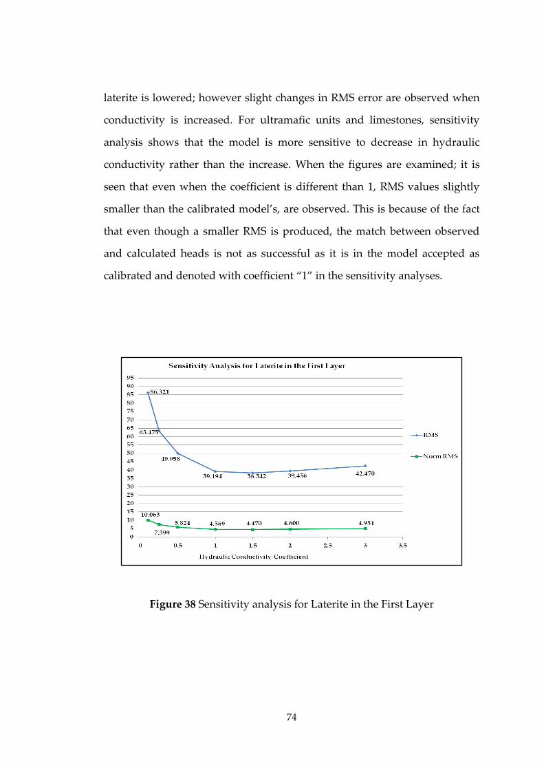
74

laterite is lowered; however slight changes in RMS error are observed when

conductivity is increased. For ultramafic units and limestones, sensitivity

analysis shows that the model is more sensitive to decrease in hydraulic

conductivity rather than the increase. When the figures are examined; it is

seen that even when the coefficient is different than 1, RMS values slightly

smaller than the calibrated model’s, are observed. This is because of the fact

that even though a smaller RMS is produced, the match between observed

and calculated heads is not as successful as it is in the model accepted as

calibrated and denoted with coefficient “1” in the sensitivity analyses.

Figure 38 Sensitivity analysis for Laterite in the First Layer

75

Figure 39 Sensitivity analysis for ultramafics in the first layer

Figure 40 Sensitivity analysis for limestones in the first layer

76

Recharge coefficients in the sensitivity analysis were 0.25, 0.5 and 1.5. As can

be depicted from Figure 41, the model is more sensitive to decrease in

recharge rather than increase in it. Furthermore, when recharge is 1.5 times

the value in the calibrated model, smaller RMS and Normalized RMS values

are obtained, however the water levels in this simulation do not match with

the observed heads as much as the calibrated model.

Figure 41 Sensitivity analysis for recharge

Finally, a sensitivity analysis was carried out for drain conductance, with

coefficients 0.1, 0.5 and 1.5. In Figure 42, it can be seen that changes in drain

conductance cause slight changes in RMS and Normalized RMS values; thus

the system is not sensitive to changes in drain conductance.

77

Figure 42 Sensitivity analysis for drain conductance

78

CHAPTER 5

DEWATERING SIMULATIONS

5.1 Methodology

The calibrated steady-state model has been applied to predict mine

dewatering requirement for the proposed 15-year mine life. In the transient

model, open-pit mining is represented by drain cells. In the active mining

areas, the drain cells were specified with drain elevations set equal to bench

elevations.

The drain cell configuration was determined by pit boundaries that are

shown in Figure 43. The progressive advancement of pits due to mine

schedule is represented in monthly time steps. The areas where excavation

has not yet started, drain elevation is set equal to 1000 m, which is high

above the water levels and is considered inactive by the software. Each active

drain cell invert elevation corresponds to different time intervals during

which excavation will reach to the pit bench elevations at the drain node. As

the excavation progresses and parts of the pits are backfilled, the

corresponding drain cells are de-activated. The aim of in-pit drain cells is to

use total outflow from drains to predict groundwater inflow rate to the mine,

which will yield the dewatering requirement.

79

Figure 43 Pits represented by drains in the model

The drain cell conductance parameter represents the resistance to flow from

saturated rocks into the drain cells, so is a critical parameter in determining

inflow into pits. In the model, 10 m2/day conductance value was selected

after trial of 1 m2/day, 5 m2/day and 1000 m2/day values. The results showed

that 1 m2/day and 5 m2/day drain conductance values were not enough to

obtain the required drawdowns and 1000 m2/day conductance value resulted

in drawdowns more than the required ones.

80

The 15-year mine life was divided into 178 time steps, each time step

corresponding to 1 month (30 days). In the first two months of 15 years, the

excavation does not start, allowing preparation of the mining infrastructure

including construction of roads, drainage and waste dump (Dagdelen and

Gungor, 2010).

5.2 Predicted Flow Rates

The open pits are located in laterite, which bears the nickel to be mined.

Hydraulic conductivity of laterites is one of the main parameters controlling

the groundwater inflow rate into open pits. In order to determine the

hydraulic conductivity of the laterites four wells were drilled into laterites

and tested. However, three of these wells were dry, leaving only one pump

tested value for hydraulic conductivity of laterites. Furthermore, this value is

expected to be an elevated value since the pump tested well is located on a

fault extending through Pig Valley and passing through this monitoring

location. Although model calibration was conducted using this value for

hydraulic conductivity of laterites, there is a significant uncertainty

associated with it. Hence, due to this uncertainty in hydraulic conductivity of

laterite, a sensitivity analysis was carried out in order to assess its affect on

the calculated inflow rates into pits. While all other parameters were kept

constant, hydraulic conductivity of laterite was multiplied by coefficients 0.1,

0.25, 0.5 and 1.5; the results are shown in Table 10. As seen in the table; when

the hydraulic conductivity of laterite in the calibrated model is used, this

flow rate is 107.58 L/s. When the hydraulic conductivity of laterite is reduced

tenfold, the flow rate decreases three fourths, to 24.42 L/s.

81

Table 10 Change of flow rates with the change of hydraulic conductivity of

laterite

Hydr. Cond.

Coefficients

of Laterite

Lat_1.5

Lat_1

Lat_0.5

Lat_0.25

Lat_0.1

Hematite

Pit

Flow Rate

(L/s) 51.47 59.41 54.37 44.38 31.49

Duration of

Dewatering

13

months

13

months

17

months

17

months

16

months

Pig Valley

Pit

Flow Rate

(L/s) 142.16 98.94 64.03 38.55 25.55

Duration of

Dewatering

143

months

140

months

102

months

102

months

102

months

South Pit

Flow Rate

(L/s) 77.40 40.81 24.75 5.07 1.57

Duration of

Dewatering

45

months

45

months

15

months

15

months

10

months

Pits

Average *

Flow Rate

(L/s) 156.93 107.58 58.41 35.54 24.42

Duration of

Dewatering

156

months

153

months

134

months

134

months

128

months

* Due to different durations of dewatering in each pit, weighted average is used in this

calculation.

The flow rates in the pits were summarized in Table 10; however as

mentioned, duration of dewatering changes in each pit. Also, the flow rates

display high variations with time in each pit. In Figure 44, time versus flow

rate plots of each pit separately and the total for all pits are given. These

results are obtained from the simulation carried out using hydraulic

conductivity of laterite in the calibrated model (Klat = 2.89x10-6 m/s). In the

82

figure, when flow rates are equal to zero there is no inflow to the pits; in this

case either no dewatering is required or the dewatering applied for another

pit produces the required drawdown in this pit too. Inferred from the figure

is that, the maximum flow rate at Hematite Pit is 111.5 L/s; at Pig Valley Pit,

319.4 L/s and at South Pit, 141.3 L/s. In this case, the total maximum flow rate

is encountered in Pig Valley pit, being equal to 319.4 L/s. This observation is

very consistent since the maximum required drawdown is also expected

from Pig Valley Pit as mentioned before. Furthermore; as given in Table 10,

the calculated average flow rate considering all the pits and their different

durations of dewatering is 107.58 L/s.

As it can be implied from Figure 44, the general trends in flow rates are in

accordance with the timewise development of pits. Increasing trends in flow

rates correspond to the progress of excavation. On the contrary, the

decreasing trends correspond to the decrease in dewatering requirement.

Despite the general increasing trends, small fluctuations in flow rates are

observed. The ascendant parts correspond to excavation of new pit benches,

and after the targeted bench elevation is reached, the bottom elevation of pit

stabilizes until the next bench excavation. Meanwhile, the dewatering rate

starts decreasing causing a descendent portion in the plot. With the

continuation of excavation of new benches, a cyclic fluctuation in the plot

occurs. When the maximum flow rate is observed at day 3000, last two stages

of Pig Valley Pit and three stages of South Pit are active; which is consistent

with the high requirement of dewatering. As previously mentioned; the

times when flow rates are zero denote that either no dewatering is required

or the dewatering applied for another pit produces the required drawdown

in this pit too.

83

Figure 44 Time versus flow rate plot for each pit separately and the total for

all pits (for the calibrated model)

Figure 45 was plotted from the results obtained from the simulation carried

out using hydraulic conductivity of laterite in the calibrated model

multiplied by 0.1 (Klat = 2.89x10-7 m/s). In this case, the maximum flow rate at

Hematite Pit is 60.6 L/s; at Pig Valley Pit, 91.9 L/s and at South Pit, 2.7 L/s.

The total maximum flow rate, being equal to 91.9 L/s, is again observed in

Pig Valley pit and this is consistent with the expectation of maximum

required drawdown in Pig Valley Pit. In this figure, the trends and cyclic

fluctuations are similarly observed as in Figure 41, the only difference is the

minor dewatering requirement of South Pit due to low initial water levels.

The dewatering applied to other pits is very effective for the water levels to

84

be lowered in South Pit; consequently, dewatering in this pit is required for a

limited time, with a very small flow rate (1.57 L/s).

Figure 45 Time versus flow rate plot for each pit separately and the total for

all pits (for one tenth of hydraulic conductivity of calibrated model)

5.3 Water Levels in the Pits

In order to check whether the water levels in the pits are lowered to the

required elevations, four representative observation locations D-1, D-2, D-3

and D-4 were selected (Figure 46). Water levels in these locations are

displayed in Figure 47, 48, 49 and 50 together with initial heads and

85

corresponding pit bench elevations as mining progresses. The displayed

results belong to the simulation carried out using hydraulic conductivity of

laterite in the calibrated model (i.e. it equals to 2.89x10-6 m/s). In Figure 47, it

is observed that in central part of Hematite Pit the initial water level is high

above the lowest bench elevation. When the timewise change of water level

and mining is examined, it is seen that the target drawdown is produced and

the water level is lowered below the pit bottom for dry mining conditions.

The first time when water level starts bouncing back corresponds to the end

of excavation in Hematite Pit (the time when drains were deactivated), the

following up and downs are effects of ongoing dewatering in other pits.

Figure 46 Observation locations

86

Figure 47 Initial head, water level and mining progress in the center of

Hematite Pit

In Figure 48, it is seen that groundwater inflow is a problem for Pig Valley

Pit for most of its excavation. It is clear that, water level is successfully

lowered below the pit bench elevations when required. The time when water

level starts to recover (day 4200) corresponds to the cessation of mining in

Pig Valley Pit.

87

Figure 48 Initial head, water level and mining progress in the center of Pig

Valley Pit

Figure 49 displays the timely change of water level and pit bench elevations

in northern part of South Pit. From the figure it can be concluded that this

part of the pit requires dewatering in the last two years of excavation, it

should be noted that South Pit is the last pit to be mined in the area. The

required drawdowns in the pit are obtained for most of the excavation time,

however at the last time steps, since dewatering in other pits lasted and

mining in the whole area is about to finish, the required water levels cannot

be reached. As mentioned before, South Pit is excavated in four stages.

Mining in this pit starts in the southern parts, and then continues in northern

areas during the last stages. For this reason, the decline in water levels before

88

the initiation of excavation is the result of ongoing dewatering in the

southern parts of this pit together with Pig Valley Pit.

Figure 49 Initial head, water level and mining progress in northern part of

South Pit

Figure 50 displays that in the central parts of South Pit, the dewatering

requirement is not excess and the required drawdown is successively

produced.

89

Figure 50 Initial head, water level and mining progress in center of South Pit

In order to assess the effects of change in hydraulic conductivity, results of

the simulation in which hydraulic conductivity of laterite is multiplied by 0.1

(i.e. it equals to 2.89x10-7 m/s) are also presented for the same observation

points (D-1, D-2, D-3 and D-4) in Figures 51, 52, 53 and 54, respectively.

When the hydraulic conductivity of the laterite is reduced by tenfold the

simulated steady-state water levels in the Pig Valley Pit and South Pit were

lowered significantly while they were slightly elevated in the Hematite Pit.

Since the heads obtained from steady-state model run were used as initial

conditions for the transient dewatering simulations, there were significant

differences in the dewatering requirements resulting from different initial

conditions. Coupled with low hydraulic conductivity of the laterite, the low

initial head produced less dewatering flow rates.

90

The results show that in Hematite Pit and Pig Valley Pit, the required

drawdown is achieved successfully as can be seen in Figures 51 and 52,

respectively. In both figures, the times when water levels start bouncing back

correspond to the cessation of excavation in these pits. In the South Pit, both

in the northern and central parts the initial water levels are below the pit

bench elevations during all the excavation time (Figures 53 and 54). At the

selected locations, dewatering requirement is not necessary but for other

regions of the South Pit there is the requirement of dewatering, however it is

far too less compared to the other pits.

Figure 51 Initial head, water level and mining progress in the center of

Hematite Pit

91

Figure 52 Initial head, water level and mining progress in the center of Pig

Valley Pit

Figure 53 Initial head, water level and mining progress in northern South Pit

92

Figure 54 Initial head, water level and mining progress in center of South Pit

93

CHAPTER 6

CONCLUSION AND RECOMMENDATIONS

The purpose of this study was to assess the dewatering requirements of

planned open pit nickel mining at Çaldağ Site in Western Turkey. With

excavation of three open pits, 15 years of mining is proposed in Çaldağ. With

the progress of mining, penetration of water table will be encountered and

this will cause groundwater inflow to the mine. For safe and efficient

conditions together with pit wall stability in the mine, dewatering is crucial.

This study was carried out to predict the rate at which the dewatering should

be accomplished.

In order to characterize the study area; a conceptual model was developed

using geology, hydrogeology, meteorology and hydrology data.

Consequently, a numerical groundwater model based on this conceptual

model was set up, using MODFLOW. After calibration of this model with

existing field data, dewatering simulations were carried out to predict the

dewatering rate. In the dewatering simulations, a transient model covering

the proposed 15-year mine life with monthly time steps was utilized. In this

model, open-pit mining was represented by drain cells, using MODFLOW

Drain Package. In the active mining areas, the drain cells were specified with

drain elevations set equal to bench elevations. The configuration of drain

cells was determined by pit boundaries, and the progressive advancement of

pits based on the mine schedule was represented in monthly time steps. The

94

purpose of using in-pit drain cells was to use the outflow from drains to

calculate the inflow rate to the mine. In order to obtain dry conditions in the

pits, the dewatering rate should be at least equal to the inflow rate into the

mine.

Based on the data from calibrated steady-state model; when all pits are taken

into account, the average flow rate was determined to be 107.58 L/s. Because

the hydraulic conductivity of laterite is one of the main parameters

controlling the flow rate into the pits and due to lack of sufficient data

regarding this parameter, it was essential to assess the impact of this

parameter on the pit inflow rates. Therefore, simulations were carried out for

a range of different laterite hydraulic conductivities (hydraulic conductivity

coefficients of 0.1, 0.25, 0.5 and 1.5 were used). In the calibrated model;

2.89x10-6 m/s, determined by pumping test, was used. A tenfold reduction in

the hydraulic conductivity of laterite (2.89x10-7 m/s) resulted in three fourths

of decrease in the flow rate (24.42 L/s).

Since nickel is extracted from the laterite, hydraulic conductivity of laterites

is one of the main parameters controlling the groundwater inflow rate into

open pits. Due to lack of sufficient data regarding hydraulic conductivity of

laterites, a sensitivity analysis was carried out and a range of flow rates were

calculated for different hydraulic conductivity values. Hence, in order to

confirm the hydraulic conductivity of laterites and obtain a realistic flow rate

for dewatering, further tests aiming the hydraulic conductivity distribution

in laterites are needed.

95

For the results of this study to be put into practice, with new simulations a

dewatering plan should be developed in future studies. During operation of

the mine while dewatering is active, the model should be continuously

updated with discharge and water level data from the dewatering system. In

addition, further modeling studies evaluating the recovery of water levels

within the pits following the cessation of mining are recommended.

96

REFERENCES

Ağartan, E., 2010, Assessment of Water Supply Impacts for A Mine Site in

Western Turkey. Master's thesis, Middle East Technical University.

Bozkurt, E., and Rojay, B., 2005, Episodic , Two-stage Neogene Extension and

Short-Term Intervening Compression in Western Turkey: Field Evidence

from the Kiraz Basin and Bozdag Horst. Geodinamica Acta, 4, 299-316.

Bozkurt, E., and Satir, M., 2000, The Southern Menderes Massif (Western

Turkey): Geochronology and Exhumation History. Geological Journal,

35(3-4), 285-296.

Bozkurt, E., and Sözbilir, H., 2004, Tectonic Evolution of the Gediz Graben:

Field Evidence for an Episodic, Two-stage Extension in Western Turkey.

Geological Magazine, 141(1), 63-79.

Bruce, I. G., 2006, Open Pit Dewatering Numerical Modelling Report, BGC

Engineering, 41 p.

Büyükakıncı, E., and Topkaya, Y. A., 2009, Extraction of Nickel from Lateritic

ores at Atmospheric Pressure with Agitation Leaching.

Hydrometallurgy, 97(1-2), 33-38. Elsevier B.V.

Çiftçi, N. B., and Bozkurt, E., 2009, Evolution of the Miocene sedimentary Fill

of the Gediz Graben, SW Turkey. Sedimentary Geology, 216(3-4), 49-79.

Elsevier B.V.

Dağdelen, K., and Güngör, A., 2010, Mine Planning and Production Schedule

of Caldag Nickel Project, 35 p.

Duru, U., 2004, Dewatering Plan and Prediction For Pit Lake Flooding for a

Quarry Site. Master's thesis, Middle East Technical University.

Farrington, V., and MacHunter, C., 2007, Hydrogeological Assessment of the

Maud Creek Gold Project. Terra, 39 p.

Göveli, A., 2006, Nickel Extraction From Gordes Laterites by Hydrochloric

Acid Leaching, Master's thesis, Middle East Technical University.

97

Harbaugh, A. W., Banta, E. R., Hill, M. C., and McDonald, M. G., 2000,

MODFLOW-2000, The U.S. Geological Survey Modular Ground-Water

Model: User Guide to Modularization Concepts and the Ground-Water

Flow Process, U.S. Geological Survey, Open-File Report 00-92.

Kuchling, K., Chorley, D., and Zawadzki, W., 2000, Hydrogeological

Modeling of Mining Operations at the Diavik Diamonds Project.

Morton, K. L., and Van Mekerk, F. A., 1993, A Phased Approach to Mine

Dewatering. Mine Water and the Environment, 12(Annual), 27-34.

Oxley, A., Sirvanci, N., and Purkiss, S., 2007, Çaldağ Nickel Laterite

Atmospheric Heap Leach Project. Metalurgija –Journal of Metallurgy

(MJoM), 13(1), 5-10.

Philippson, A., 1915, Reisin Und Forsehungen in Westliehen Klainasien: Pet.

Mitt. Erg. M. 167, 173, 177, 1980, Cotha.

Schlumberger Water Services, Visual MODFLOW – Dynamic Groundwater

Flow and Contaminant Transport Modeling Software, 2010, Canada.

Shepherd, R., 1993, Ancient Mining. Elsevier, 494 p; Elsevier B.V.

Singh, R. N., and Reed, S. M., 1988, Mathematical Modelling for Estimation

of Minewater Inflow to a Surface Mining Operation. International

Journal of Mine Water, 7(3), 1-33.

Soil Conservation Service, 1964, SCS National Engineering Handbook,

Section 4: Hydrology, Updated 1972, U.S. Department of Agriculture,

Washington D.C.

Thorne, R., Herrington, R., and Roberts, S., 2009, Composition and origin of

the Çaldağ oxide nickel laterite, W. Turkey. Mineralium Deposita, 44(5),

581-595.

University of Stuttgart, Institute of Applied and Experimental Mechanics,

Boundary Element Methods, http://www.iam.uni-

stuttgart.de/bem/home_bem_introduc.html (accessed September 2,

2011).

Williamson, S., and Vogwill, R. I. J., 2001, Dewatering In the Hot

Groundwater Conditions at Lihir Gold.

98

Wolkersdorfer, C., 2008, Water Management at Abandoned Flooded

Underground Mines. Quality Assurance, 465 p, Springer.

Yanik, G., Uz, B., and Esenli, F., 2006, Turgutlu ( Manisa ) yöresi Neojen

çökellerinin jeolojisi. İTÜ Dergisi, 5(2), 49-58.

Yazıcıgil, H., 2008, Hydrogeological Characterization of Çaldağ Nickel Mine

Project Area, Sardes Nikel Madencilik A.Ş. Quality, 128 p.

Yilmaz, Y., Genc, S. C., Gürer, F., Bozcu, M., Yılmaz, K., Karacık, Z., and

Altunkaynak, S., 2000, When Did the Western Anatolian Grabens Begin

to Develop?, Geological Society, London, Special Publications, 173(1),

353-384.