University of Calgary

PRISM: University of Calgary's Digital Repository

Graduate Studies The Vault: Electronic Theses and Dissertations

2013-08-21

Assessment of corrosion defects on high-strength

steel pipelines

Xu, Luyao

Xu, L. (2013). Assessment of corrosion defects on high-strength steel pipelines (Unpublished

doctoral thesis). University of Calgary, Calgary, AB. doi:10.11575/PRISM/25027

http://hdl.handle.net/11023/883

doctoral thesis

University of Calgary graduate students retain copyright ownership and moral rights for their

thesis. You may use this material in any way that is permitted by the Copyright Act or through

licensing that has been assigned to the document. For uses that are not allowable under

copyright legislation or licensing, you are required to seek permission.

Downloaded from PRISM: https://prism.ucalgary.ca

UNIVERSITY OF CALGARY

Assessment of corrosion defects on high-strength steel pipelines

by

Luyao Xu

A THESIS

SUBMITTED TO THE FACULTY OF GRADUATE STUDIES

IN PARTIAL FULFILMENT OF THE REQUIREMENTS FOR THE

DEGREE OF DOCTOR OF PHILOSOPHY

DEPARTMENT OF MECHANICAL AND MANUFACTURING ENGINEERING

CALGARY, ALBERTA

AUGUST, 2013

© Luyao Xu 2013

Abstract

With the rapidly increasing energy demand, the oil/gas production and pipeline

activities have been found in remote regions, such as the Arctic and sub-Arctic regions in

North America, which are featured with geological hazards and are prone to large ground

movement. The soil induced strain, combined with internal pressure, results in a complex

stress/strain condition on pipelines, especially at corrosion defects. It has been

demonstrated that the presence of corrosion defect constitutes one of the main threats to

pipeline safety. The local stress concentration developed at defect further accelerates the

localized corrosion. Moreover, the applied cathodic protection (CP) can be shielded, or at

least partially shielded, at corrosion defect. To date, there has been no systematic

investigation on the synergism of mechanical and electrochemical factors on localized

corrosion reaction at defect. The intrinsic science of this problem has remained unknown,

and assessing and predictive models that can be used in practice for pipeline integrity

management have been lacking. In this research, various macro- and micro-

electrochemical measurements, mechanical testing, and numerical simulation were

combined to study the synergism of internal pressure, soil strain and local stress

concentration on corrosion at defect on X100 high-strength steel pipelines, and develop

theoretical concepts and predictive models to provide guidelines and recommendations to

industry for an improved integrity management of pipelines.

A mechano-electrochemical (M-E) effect concept, which was built upon the

mechanical-electrochemical interaction on metallic corrosion, is proposed to illustrate

quantitatively pipeline corrosion under complex stress/strain conditions. Under elastic

ii

deformation, the mechanical-electrochemical interaction would not affect pipeline

corrosion at a detectable level. However, the plastic formation is able to enhance pipeline

corrosion remarkably. Quantitative relationships between the electrochemical potential of

steel and the elastic and plastic strains are derived, which guide the mechanistic aspects

of the M-E effect of pipeline corrosion.

A finite element (FE) model is developed to quantify the M-E effect of pipeline

corrosion through a multi-physical fields coupling simulation that analyses the solid

mechanics field in steel, electrochemical reactions at the steel/solution interface and the

electric field in both solution and the steel. Simulation results demonstrate that the

corrosion at defect is composed of a series of local galvanic cells, where the region with a

high stress, such as the defect center, serves as anode and that under the low stress, such

as the sides of the defect, as cathode.

While CP is applied on pipelines for corrosion prevention, a potential drop can be

developed inside the defect due to both the solution resistance effect and the current

dissipation effect. As a consequence, the CP potential is shielded, at least partially, at the

defect bottom, reducing the effectiveness of CP for corrosion protection at defects.

Empirical equations are derived to enable determination of the potential drop inside

defect, and thus the potential and current density distributions in the defect while CP is

applied on the pipeline. They are capable of assessing conveniently for industry the CP

effectiveness at corrosion defects and the further corrosion scenario on pipelines.

Furthermore, the present industry models, such as ASME B31G, the modified B31G

and the DNV model, for prediction of pipeline failure pressure were evaluated. It is

found that the industry models do not apply for pipelines made of high-strength steels,

iii

such as X100 steel, and contain corrosion defect with complex geometries, and thus do

not provide accurate results. A new, FE-based model, named UC model, is developed to

enable accurate prediction of failure pressure of pipelines made of various grades of steel

in the presence of corrosion defect under synergistic effect of internal pressure and soil

strain. The results predicted by UC model has been echoed by the actual experiences in

the field.

Finally, a novel FE model is developed, at the first time in this area, to enable

assessment and prediction of the time-dependent growth of corrosion defect on pipelines.

The synergistic effects of local stress concentration, corrosion reaction and the defect

geometry are critical to the defect growth. The presence of the M-E effect results in an

accelerating corrosion at the defect center, generating a geometrical flaw and enhancing

the local stress level. The developed model can predict the time dependences of local

stress, corrosion rate and the geometrical shape of corrosion defect, thus providing a

promising alternative for assessing the long-term growth of corrosion defect on pipelines.

iv

Acknowledgements

I would like to express my sincere gratitude to my supervisor, Dr. Frank Cheng for

his constant guidance, encouragement, and support throughout my whole program. His

deep love and perception of science, his persistent endeavour for searching for the truth,

and his consistent efforts at achieving perfection have always inspired and helped me

carry out this research project.

Thanks are also extended to the members in my group, Mr. Yanghao Tang, Drs.

Yang Hu, Ruiling Jia, Ruijing Jiang and Dong Han, Yang Yang, Xin Su, Zhong Li, and

those whose names cannot all be listed here, for their helps and valuable discussions in

this work.

The generous financial supports from Canada Research Chairs Program and Pipeline

Engineering Center of the University of Calgary through the IPCF Research Grant

Program are highly appreciated, and make this work possible.

v

Dedication

This work is dedicated to my parents and my wife Xin Su, for their incessant support.

vi

Table of Contents

Abstract .......................................................................................................................... ii Acknowledgements ......................................................................................................... v Dedication ...................................................................................................................... vi Table of Contents ..........................................................................................................vii List of Tables.................................................................................................................. xi List of Figures and Illustrations .....................................................................................xii List of Symbols, Abbreviations and Nomenclature ........................................................ xx

Chapter One: Introduction ............................................................................................... 1 1.1 Research background ............................................................................................. 1 1.2 Objectives .............................................................................................................. 3 1.3 Contents of thesis ................................................................................................... 4

Chapter Two: Literature review ....................................................................................... 6 2.1 Development of high-strength pipeline steels ......................................................... 6

2.1.1 Environmental challenges .............................................................................. 6 2.1.2 Strain-based design methodology ................................................................... 8 2.1.3 Requirements of mechanical properties for high strength steels .................... 10 2.1.4 Metallurgical design and processing of high strength steels .......................... 12 2.1.5 Effect of welding ......................................................................................... 15

2.2 Corrosion of pipelines .......................................................................................... 15 2.2.1 Overview of pipeline corrosion .................................................................... 15 2.2.2 General corrosion......................................................................................... 17 2.2.3 Pitting corrosion .......................................................................................... 17 2.2.4 Stress corrosion cracking ............................................................................. 19

2.3 Inspection technologies for pipeline defects ......................................................... 20 2.3.1 Tools for metal-loss (corrosion) type defects ................................................ 20 2.3.2 Tools for crack-like defects .......................................................................... 22 2.3.3 Tools for geometrical deformation ............................................................... 23

2.4 Assessment of pipeline defects ............................................................................. 24 2.5 Prediction of failure pressure of pipelines containing defects ............................... 27

2.5.1 Overview of defect assessment models ........................................................ 27 2.5.2 Limitations of the present assessment models .............................................. 31

2.6 Prediction of remaining service life of pipelines containing defects ...................... 31

Chapter Three: Research methodology .......................................................................... 34 3.1 Materials and solutions ........................................................................................ 34 3.2 Mechanical tensile testing .................................................................................... 36 3.3 Conventional macro-electrochemical measurements ............................................ 37 3.4 Micro-electrochemical measurements .................................................................. 39 3.5 Surface characterization ....................................................................................... 42

Chapter Four: Pipeline corrosion under mechanical-electrochemical interaction - elastic deformation ................................................................................................ 43

4.1 Results ................................................................................................................. 44

vii

4.1.1 Mechanical testing ....................................................................................... 44 4.1.2 LEIS measurements ..................................................................................... 45 4.1.3 Corrosion potential and EIS measurements .................................................. 45 4.1.4 FEA of stress and strain distributions on the steel specimens ........................ 50 4.1.5 Surface characterization ............................................................................... 51

4.2 Discussion ........................................................................................................... 52 4.2.1 Electrochemical corrosion behavior of X100 steel in NS4 solution............... 52 4.2.2 Effect of static elastic stress/strain on corrosion of the steel.......................... 54 4.2.3 Effect of dynamic elastic stress/strain on corrosion of X100 steel................. 57 4.2.4 Implications on pipeline corrosion and its control in the field ....................... 59

4.3 Summary ............................................................................................................. 59

Chapter Five: Pipeline corrosion under mechanical-electrochemical interaction - plastic deformation ............................................................................................... 61

5.1 Results ................................................................................................................. 61 5.1.1 Mechanical testing ....................................................................................... 61 5.1.2 Conventional macro-electrochemical measurements .................................... 63 5.1.3 LEIS and SVET measurements .................................................................... 68 5.1.4 FE analysis of the stress/strain distributions ................................................. 70

5.2 Discussion ........................................................................................................... 72 5.2.1 Effect of elastic deformation on corrosion of the steel .................................. 73 5.2.2 Effect of plastic deformation on corrosion of the steel .................................. 74 5.2.3 Corrosion of steel during tensile testing ....................................................... 76 5.2.4 Corrosion of pipelines with a non-uniform plastic stress/strain distribution .. 78

5.3 Summary ............................................................................................................. 79

Chapter Six: Development of a finite element model for simulation and prediction of the M-E effect at corrosion defects ........................................................................ 80

6.1 Numerical simulation and analysis ....................................................................... 80 6.1.1 Initial and boundary geometrical parameters ................................................ 80 6.1.2 Multi-physical fields coupling FE simulation of M-E effect of pipeline

corrosion ...................................................................................................... 85 6.1.3 Validity of FE simulation with experimental data ......................................... 88

6.2 Results ................................................................................................................. 89 6.2.1 FE simulation of the stress concentration at corrosion defect and the

potential and net current density distributions in solution.............................. 89 6.2.2 FE simulation of linear distributions of stress at the bottom of corrosion

defect ........................................................................................................... 94 6.2.3 FE simulation of linear distributions of corrosion potential and

anodic/cathodic current densities at corrosion defect .................................... 95 6.3 Discussion ......................................................................................................... 103

6.3.1 Effect of tensile strain and defect depth on stress distribution at corrosion defect ......................................................................................................... 103

6.3.2 M-E effect on corrosion potential of steel and the potential field distribution in solution................................................................................ 104

6.3.3 M-E effect on anodic/cathodic current density and the current field distribution in solution................................................................................ 106

viii

6.3.4 Implications on pipeline corrosion and the risk assessment ........................ 108 6.4 Summary ........................................................................................................... 109

Chapter Seven: Experimental and numerical studies of the effectiveness of cathodic protection at corrosion defect on pipelines .......................................................... 111

7.1 Numerical simulation and analysis ..................................................................... 112 7.2 Results ............................................................................................................... 113

7.2.1 Distributions of potential and current density on the steel electrode ............ 113 7.2.2 Distributions of potential and current density inside defects ....................... 116 7.2.3 Numerical simulation of potential and current fields at cylindrical defects . 116 7.2.4 Numerical simulation of potential and current fields at ellipsoidal defects .. 119 7.2.5 Numerical simulation of potential and current fields at ellipsoidal defects

under various applied cathodic potentials ................................................... 123 7.3 Discussion ......................................................................................................... 126

7.3.1 Error analysis of the experimental and numerical results ............................ 126 7.3.2 Effect of defect geometry on potential distribution ..................................... 127 7.3.3 Effect of defect geometry on current density distribution ........................... 130 7.3.4 Implications on CP performance on pipelines and defect assessment.......... 132

7.4 Summary ........................................................................................................... 135

Chapter Eight: Prediction of failure pressure of pipelines under synergistic effects of internal pressure, soil strain and corrosion defects ............................................... 136

8.1 Models for reliability assessment and failure pressure prediction of pipelines .... 138 8.1.1 Present industry models ............................................................................. 138 8.1.2 FE modeling assessment ............................................................................ 140 8.1.3 The FE simulation...................................................................................... 141

8.2 Results ............................................................................................................... 144 8.2.1 Prediction of failure pressure of pipelines by individual models ................. 144 8.2.2 Determination of von Mises stress on pipelines in the presence and

absence of corrosion defect ........................................................................ 151 8.2.3 Distribution of plastic deformation and von Mises stress at corrosion

defect ......................................................................................................... 155 8.2.4 Effect of soil strain on plastic deformation of the corroded pipe ................. 157

8.3 Discussion ......................................................................................................... 159 8.3.1 Evaluation of the industry models in prediction of pipeline failure pressure159 8.3.2 Effect of corrosion defect on stress and strain distributions on pipeline ...... 161 8.3.3 Effect of soil strain on failure pressure and plastic deformation of

pipelines ..................................................................................................... 163 8.4 Summary ........................................................................................................... 164

Chapter Nine: Long-term prediction of growth of corrosion defect on pipelines ........... 167 9.1 Numerical simulation and analysis ..................................................................... 168

9.1.1 Initial and boundary conditions .................................................................. 168 9.1.2 Interactions of mechanical, electrical and electrochemical corrosion multi-

physical fields ............................................................................................ 169 9.2 Results ............................................................................................................... 171

ix

9.2.1 Comparison of long-term growth of corrosion defect in the absence and presence of M-E effect ............................................................................... 171

9.2.2 Effect of defect geometry on long-term growth of corrosion defect ............ 179 9.2.3 Effect of operating pressure on long-term growth of corrosion defect ......... 182 9.2.4 Effect of CP on long-term growth of corrosion defect ................................ 184

9.3 Discussion ......................................................................................................... 186 9.3.1 The M-E effect on localized corrosion at defect and its growth .................. 186 9.3.2 Effect of geometry of corrosion defect on its growth .................................. 187 9.3.3 Effects of operating pressure and CP on growth of corrosion defect ........... 189 9.3.4 Implications on pipeline risk assessment of surface defects ........................ 190

9.4 Summary ........................................................................................................... 191

Chapter Ten: Conclusions and recommendations ......................................................... 193 10.1 Conclusions ..................................................................................................... 193 10.2 Recommendations ............................................................................................ 196

Research publications in peer-reviewed journals .......................................................... 197

References ................................................................................................................... 198

x

List of Tables

Table 2.1. Recommended methods for defect assessment on pipelines ........................... 25

Table 2.2. Failure pressure models for pipeline containing corrosion defects. ................. 30

Table 3.1. Chemical composition of X100 steel (wt.%).................................................. 35

Table 4.1. Electrochemical parameters fitted from EIS data measured under various tensile stresses........................................................................................................ 53

Table 4.2. Electrochemical parameters fitted from EIS data measured under various compressive stresses .............................................................................................. 53

Table 5.1. Mechanical properties of X100 steel specimen with various pre-strains. ........ 62

Table 6.1: The initial electrochemical parameters for FE simulation derived from Fig. 6.2.......................................................................................................................... 84

Table 8.1. Mechanical properties of various grades of pipeline steel. ........................... 142

Table 8.2. Geometry of line pipe for the FE simulation. ............................................... 142

Table 8.3. Geometry of corrosion defects investigated in this work .............................. 142

Table 8.4. Failure pressure of the steel pipe with a corrosion defect of 20% of pipe wall thickness and 200 mm in length determined by the individual models .......... 145

Table 8.5. Failure pressure of the steel pipe with a corrosion defect of 40% of pipe wall thickness and 200 mm in length determined by the individual models .......... 146

Table 8.6. Failure pressure of the steel pipe with a corrosion defect of 60% of pipe wall thickness and 200 mm in length determined by the individual models .......... 146

Table 8.7. Failure pressure of the steel pipe with a corrosion defect of 80% of pipe wall thickness and 200 mm in length determined by the individual models .......... 146

Table 8.8. Failure pressures of X80 steel pipe containing a corrosion defect with 80% of pipe wall loss thickness under applied tensile pre-strains in longitudinal direction predicted by the UC model .................................................................... 158

Table 8.9. Failure pressures of X80 steel pipe containing a corrosion defect with 80% of pipe wall thickness under applied compressive pre-strains in longitudinal direction predicted by the UC model .................................................................... 158

xi

List of Figures and Illustrations

Fig. 2.1. Examples of geologic hazards from seismic, soil instability, discontinuous permafrost, and shallow water iceberg scouring. ......................................................7

Fig. 2.2. Mechanisms of frost heave and thaw settlement in permafrost area ....................7

Fig. 2.3. Comparison of stress-based design and strain-based design criteria ....................9

Fig. 2.4. Yielding types of pipeline steels and the influence on buckling. ....................... 11

Fig. 2.5. Development of high strength pipeline steels ................................................... 13

Fig. 2.6. Relationships between tensile strength and uniform elongation or absorbed energy in Charpy-V notch impact test .................................................................... 14

Fig. 2.7. Schematic diagram of accelerated cooling process to obtain a dual-phase microstructure ........................................................................................................ 14

Fig. 2.8. Canadian National Energy Board (NBE) regulated pipeline rupture causes between 1991 and 2009 .......................................................................................... 16

Fig. 2.9. (a) SEM image of MnS inclusion; (b) stress field this inclusion for an applied stress of 350 MPa ...................................................................................... 18

Fig. 2.10. Principle of Magnetic flux leakage (MFL) ..................................................... 21

Fig. 2.11. Principles of ultrasonic wall measurement and crack detection ....................... 21

Fig. 2.12. Principle of Electromagnetic Acoustic transducers (EMAT) ........................... 22

Fig. 2.13. Flowchart showing elements of the EB-IMP process ...................................... 26

Fig. 2.14, Dimensions of corrosion defect ...................................................................... 29

Fig. 3.1. Schematic diagrams of various types of specimens used in this work: (a) and (b) flat-plate specimens; (c) rod specimen; (d) rectangular specimen containing artificial defects. .................................................................................................... 36

Fig. 3.2. Schematic diagram of the experimental setup for various macro-electrochemical measurements on X100 steel specimen. ........................................ 38

Fig. 3.3. Schematic diagram of the experimental setup of micro-electrochemical measurements on the steel specimen through the M370 scanning electrochemical workstation. ........................................................................................................... 40

Fig. 3.4. Schematic diagram of the home-made potential microprobe for potential measurement at defects. ......................................................................................... 40

xii

Fig. 3.5. Time dependence of the open-circuit potential of the home-made potential microprobe vs. SCE in NS4 solution. ..................................................................... 41

Fig. 4.1. Engineering stress-strain curve of X100 steel specimen measured in air. .......... 44

Fig. 4.2. LEIS line scanning measurements on the flat steel specimen (Fig. 3.1a) after 2 days of immersion in NS4 solution under different test conditions: (a) no load applied on the specimen; (b) 2000 N force applied before immersion; and (c) 2000 N force applied after immersion. ................................................................... 46

Fig. 4.3. Corrosion potential of X100 steel rod tensile specimen (Fig. 3.1c) in NS4 solution during dynamic loadings (loading applied at 300 s) from 0 to tensile-600 MPa or compressive-600 MPa, respectively. ................................................... 46

Fig. 4.4. Nyquist diagrams of the steel rod tensile specimen after 2 days of static pre-stressing at 0, tensile 600 MPa and compressive 600 MPa in NS4 solution............. 47

Fig. 4.5. Nyquist diagrams of X100 steel specimen under dynamic tensile stress increasing from 0 to 200, 400 and 600 MPa in NS4 solution, where the stress was applied after 2 days of immersion in the solution and increased from 0 to the designated value in several seconds. ....................................................................... 48

Fig. 4.6. Nyquist diagrams of X100 steel under compressive stress increasing from 0 to 200, 400, 600 MPa in NS4 solution. ................................................................... 49

Fig. 4.7. The von Mises stress distribution of the flat specimen under a tensile force of 2000 N. .................................................................................................................. 49

Fig. 4.8. The von Mises stress and strain distribution along the red-marked line on the flat specimen. ......................................................................................................... 50

Fig. 4.9. von Mises stress distribution on the rod specimen under tensile or compressive force of 19000 N. ............................................................................... 51

Fig. 4.10. SEM view of corrosion product formed on the surface of X100 steel specimen after tensile test in NS4 solution. ............................................................ 52

Fig. 5.1. Engineering stress-strain curves of X100 steel with various pre-strains. ........... 62

Fig. 5.2. The percentage of change in yield strength, ultimate tensile strength and fraction strain of X100 steel rod specimen as a function of pre-strain. .................... 63

Fig. 5.3. Time dependence of corrosion potential of X100 steel rod specimen under various pre-strains in NS4 solution. ........................................................................ 64

Fig. 5.4. Time dependence of stress and corrosion potential of 0% pre-strained X100 steel specimen during tensile testing at a strain rate of 1×10-4/s in NS4 solution. .... 64

xiii

Fig. 5.5. Time dependence of stress and corrosion potential of the 3.918% pre-strained X100 steel during tensile testing at a strain rate of 1×10-4/s in NS4 solution. ................................................................................................................. 65

Fig. 5.6. Time dependence of coupling potential and current density flowing between deformed and non-deformed specimens in NS4 solution. ....................................... 67

Fig. 5.7. Nyquist diagrams measured on X100 steel rod specimen that at open circuit potential under various pre-strains in NS4 solution. ................................................ 67

Fig. 5.8. Current densities measured on X100 steel rod specimen that is polarized at -1 V (SCE) under various pre-strains in NS4 solution. ............................................. 68

Fig. 5.9. LEIS line scanning measurement on the X100 steel flat specimen in NS4 solution. ................................................................................................................. 69

Fig. 5.10. SVET line scanning measurement on the X100 steel flat specimen in NS4 solution. ................................................................................................................. 69

Fig. 5.11. von Mises stress distribution on the flat plate specimen under a tensile force of 2750 N. .............................................................................................................. 70

Fig. 5.12. Plastic strain distribution of the flat plate specimen under a tensile force of 2750 N. .................................................................................................................. 71

Fig. 5.13. von Mises stress and plastic strain distributions along the red line marked on the flat plate specimen under a tensile force of 2750 N. ..................................... 71

Fig.5.14. Theoretical calculation of the electrochemical equilibrium potential shift as a function of plastic strain of the steel specimen with various initial dislocation densities. ................................................................................................................ 76

Fig. 6.1. The geometrical model of the steel pipe containing a corrosion defect for FE simulation (a) 3D model, (b) 2D model. ................................................................. 81

Fig. 6.2. Potentiodynamic polarization curve measured on X100 steel in NS4 solution. .............................................................................................................................. 85

Fig. 6.3. Comparison of the experimental data and FE simulating results of corrosion potential of X100 steel in NS4 solution as a function of von Mises stress. .............. 88

Fig. 6.4. Comparison of experimental data and the FE simulating results of net current density of X100 steel in NS4 solution as a function of von Mises stress. ................ 89

Fig. 6.5. Distributions of the potential field in NS4 solution and von Mises stress at the corrosion defect (11.46 mm in depth) under various longitudinal strains. .......... 90

xiv

Fig. 6.6. Distributions of the potential field in NS4 solution and von Mises stress at the corrosion defect with various depths under a fixed 0.3% longitudinal tensile strain. ..................................................................................................................... 91

Fig. 6.7. Distributions of net current density in NS4 solution and von Mises stress at corrosion defect (11.46 mm in depth) on the pipe wall under various longitudinal tensile strains. ........................................................................................................ 92

Fig. 6.8. Distributions of net current density in solution and von Mises stress at corrosion defect with various depths under a fixed 0.3% longitudinal strain. .......... 93

Fig. 6.9. Linear distribution of von Mises stress along the bottom of the 11.46 mm deep corrosion defect on the pipe under various longitudinal tensile strains. ........... 94

Fig. 6.10. Linear distribution of von Mises stress along the bottom of corrosion defect with various depths under 0.3% longitudinal tensile strain. .................................... 95

Fig. 6.11. Linear distribution of corrosion potential along the bottom of corrosion defect with 11.46 mm in depth on the pipe under various longitudinal tensile strains in NS4 solution. .......................................................................................... 96

Fig. 6.12. Linear distribution of corrosion potential along the bottom of corrosion defect with various depths in NS4 solution where a 0.3% longitudinal tensile strain is applied. ..................................................................................................... 97

Fig. 6.13. Linear distribution of anodic current density along the bottom of the 11.46 mm corrosion defect under various longitudinal tensile strains in NS4 solution. ..... 98

Fig. 6.14. Linear distribution of anodic current density along the bottom of corrosion defect with various depths in NS4 solution, where a 0.3% longitudinal tensile strain is applied. ..................................................................................................... 98

Fig. 6.15. Linear distribution of cathodic current density along the bottom of the 11.46 mm corrosion defect under various longitudinal tensile strains in NS4 solutions. ............................................................................................................. 100

Fig. 6.16. Linear distribution of cathodic current density along the bottom of corrosion defect with various depths under 0.3% longitudinal tensile strain. ......... 100

Fig. 6.17. Linear distribution of net current density along the bottom of corrosion defect (11.46 mm in depth) under various longitudinal tensile strains in NS4 solution. ............................................................................................................... 101

Fig. 6.18. Linear distribution of net current density along the bottom of corrosion defect with various depths and under 0.3% longitudinal tensile strain in NS4 solution. ............................................................................................................... 102

xv

Fig. 6.19. Anodic and cathodic current densities at the bottom of corrosion defects as a function of von Mises stress. ............................................................................. 103

Fig. 7.1. 3D cross-section view of X100 steel specimen containing various defects for FE modeling. ....................................................................................................... 112

Fig. 7.2. Linear distribution of potential across defects on X100 steel electrode surface in NS4 solution without and with CP of -1 V(SCE) measured experimentally by the microprobe and simulated numerically. ............................. 114

Fig. 7.3. Distribution of current density across defects on the steel electrode under -1 V(SCE) potential in NS4 solution. ....................................................................... 115

Fig. 7.4. Potential distribution inside defects with various widths in NS4 solution when the steel is under -1 V(SCE) CP potential.................................................... 115

Fig. 7.5. 2D cross-sectional view of the potential field in solution where the X100 steel electrode under -1 V(SCE) potential is immersed (unit: V). .......................... 117

Fig. 7.6. 3D view of distributions of potential (a. unit: V) and Fe dissolution current density (b. unit: µA/cm2) when the steel electrode is under -1 V(SCE) in NS4 solution. ............................................................................................................... 118

Fig. 7.7. 2D potential distribution at ellipsoid-shape defects with various depth (d) and width (w) under CP of -1 V (SCE) in NS4 solution (unit: mm). ..................... 120

Fig. 7.8. Local potential at corrosion defects with various widths and depths on X100 steel under -1 V(SCE) in NS4 solution. ................................................................ 120

Fig. 7.9. Fe dissolution current density at corrosion defects with various widths and depths on X100 steel under -1 V(SCE) in NS4 solution. ....................................... 121

Fig. 7.10. Hydrogen evolution current density at defects with various widths and depths on X100 steel under -1 V(SCE) in NS4 solution. ....................................... 122

Fig. 7.11. Potential at the bottom of defect with 4 mm depth and various widths as a function of applied cathodic potential in NS4 solution. ......................................... 124

Fig. 7.12. Fe dissolution current density at the bottom of defects with 4 mm depth and various widths as a function of applied cathodic potential in NS4 solution. .......... 124

Fig. 7.13. Hydrogen evolution current density at the bottom of defects with 4 mm depth and various widths as a function of applied cathodic potential in NS4 solution. ............................................................................................................... 125

Fig. 7.14. Conceptual model is developed to illustrate mechanistically generation of a potential drop in defect......................................................................................... 128

xvi

Fig. 8.1. Typical stress-strain curves of X65, X80 and X100 steels. ............................. 143

Fig. 8.2. 3-D modeling of the pipe with a corrosion defect: (a) full model (b) a quarter model. .................................................................................................................. 144

Fig. 8.3. Effect of the defect depth on RE determined by industry models for X65 steel. .................................................................................................................... 148

Fig. 8.4. Effect of the defect depth on RE of the industry models for X80 steel. ........... 148

Fig. 8.5. Effect of the corrosion depth on RE of the industry models for X100 steel. .... 149

Fig. 8.6. Standard deviation of RE of industry models under various corrosion defect depths. ................................................................................................................. 150

Fig. 8.7. Standard deviation of RE of industry models as a function of the steel grade. 151

Fig. 8.8. Local von Mises stresses of the inner and outer surfaces of X80 steel pipe as a function of internal pressure in the presence and absence of a corrosion defect of 20% of pipe wall thickness............................................................................... 152

Fig. 8.9. Local von Mises stresses of the inner and outer surfaces of X80 steel pipe as a function of internal pressure in the presence and absence of a corrosion defect of 80% of pipe wall thickness............................................................................... 153

Fig. 8.10. Effective plastic strain of the outer and inner surfaces of X80 steel pipe in the absence and presence of a corrosion defect with 20% of pipe wall thickness. . 154

Fig. 8.11. Effective plastic strain of the outer and inner surfaces of X80 steel pipe in the absence and presence of a corrosion defect with 80% of pipe wall thickness. . 155

Fig. 8.12. Front views of the plastic deformation area on a pressurized X80 steel pipe (at 18 MPa) containing a corrosion defect with different depths. .......................... 156

Fig. 8.13. Cross-sectional views of the plastic deformation area on a pressurized X80 steel pipe (at 18 MPa) containing a corrosion defect with different depths. ........... 156

Fig. 8.14. Distributions of von Mises stress on the pressurized pipe at 18 MPa containing a corrosion defect with various depths................................................. 157

Fig. 8.15. Distribution of plastic deformation on X80 steel pipe containing a corrosion defect with 80% of pipe wall thickness under different strain conditions (from left to right: no pre-strain, 0.2% tensile strain, 0.2% compressive strain). ............. 159

Fig. 9.1. The geometrical model of the steel pipe containing a corrosion defect for FE simulation. ........................................................................................................... 168

xvii

Fig. 9.2. Distributions of von Mises stress, net current density and the vector fields at the defect in the absence and presence of the M-E effect (Initial defect width 8 mm and depth 2 mm, operating pressure 20 MPa). ............................................... 172

Fig. 9.3. Growth of corrosion defect in NS4 solution in the absence and presence of M-E effect (Initial defect width 8 mm and depth 2 mm, operating pressure 20 MPa). ................................................................................................................... 173

Fig. 9.4. Distributions of von Mises stress along the bottom of corrosion defect in the absence and presence of M-E effect (Initial defect width 8 mm and depth 2 mm, operating pressure 20 MPa). ................................................................................. 173

Fig. 9.5. Distribution of corrosion potential along the bottom of corrosion defect in the absence and presence of M-E effect (Initial defect width 8 mm and depth 2 mm, operating pressure 20 MPa). ......................................................................... 174

Fig. 9.6. Distribution of anodic current density along the bottom of corrosion defect in the absence and presence of M-E effect (Initial defect width 8 mm and depth 2 mm, operating pressure 20 MPa). ......................................................................... 175

Fig. 9.7. Distribution of cathodic current density along the bottom of corrosion defect in the absence and presence of M-E effect (Initial defect width 8 mm and depth 2 mm, operating pressure 20 MPa). ......................................................................... 176

Fig. 9.8. The von Mises stress at the defect edge and its center as a function of time in the absence and presence of M-E effect (Initial defect width 8 mm and depth 2 mm, operating pressure 20 MPa). ......................................................................... 177

Fig. 9.9. Anodic current density (or corrosion rate) at the defect edge and its center as a function of time in the absence and presence of M-E effect (Initial defect width 8 mm and depth 2 mm, operating pressure 20 MPa). ............................................ 178

Fig. 9.10. Distribution of von Mises stress at corrosion defects with varied geometries at 0, 10 and 20 years in the presence of M-E effect (Operating pressure 20 MPa, Color legend: von Mises stress, MPa). ................................................................. 180

Fig. 9.11. The von Mises stress at the center of defects with various widths (depth in 2 mm) as a function of time in the presence of M-E effect (Operating pressure 20 MPa). ................................................................................................................... 180

Fig. 9.12. Time dependence of anodic current density (or corrosion rate) at the center of corrosion defects with varied widths in the presence of M-E effect (Operating pressure 20 MPa). ................................................................................................ 182

Fig. 9.13. Time dependence of the von Mises stress at the defect center under various operating pressures in the presence of M-E effect (Initial defect width 8 mm and depth 2 mm). ........................................................................................................ 183

xviii

Fig. 9.14. Time dependence of the anodic current density (or corrosion rate) at the defect under various operating pressures in the presence of M-E effect (Initial defect width 8 mm and depth 2 mm). ................................................................... 184

Fig. 9.15. The von Mises stress at the defect center under various CP potentials in the presence of M-E effect (Initial defect width 8 mm and depth 2 mm, operating pressure 20 MPa). ................................................................................................ 185

Fig. 9.16. Anodic current density (or corrosion rate) at the defect center under various CP potentials in the presence of M-E effect (Initial defect width 8 mm and depth 2 mm, operating pressure 20 MPa). ...................................................................... 186

xix

List of Symbols, Abbreviations and Nomenclature

Symbol Definition

A Projected area of defect

AC Alternating Current

API American Petroleum Institute

ASME American Society of Mechanical Engineers

ASTM American Society for Testing and Materials

ba Anodic Tafel slope

bc Cathodic Tafel slope

c wall thickness (Eq. 9.1)

BS British Standard

CE Counter Electrode

CP Cathodic Protection

d Depth of defect

D Outer diameter of pipeline

DPP Dual-Phase Process

DLQ Delayed Quench Process

DNV Det Norske Veritas

D/t Diameter to wall thickness ratio

E Young’s modulus

EB-IMP Engineering-Based Integrity Management Program

EIS Electrochemical Impedance Spectroscopy

EMAT Electromagnetic Acoustic Transducers

xx

F Faraday’s constant (96485 C/mol)

FE Finite Element

FEA Finite Element Analysis

FFS Fitness-For-Service

GPS Global Positioning System

HAZ Heat Affected Zone

ia Anodic current density

ic Cathodic current density

i0 exchange current density

ILI In-Line Inspection

L Length of defect

LEIS Localized Electrochemical Impedance Spectroscopy

M Folias bulging factor

MAC Mild Accelerated Cooling

M-E Mechano-Electrochemical

MFL Magnetic Flux Leakage

MUMPS Multi-Frontal Massively Parallel Sparse

n number of dislocations in a dislocation pile-up

NEB National Energy Board

N0 initial density of dislocations

Nmax maximum dislocation density

ΔN density of new dislocations

PDAM Pipeline Defect Assessment Manual

xxi

PF Failure pressure

Pi Internal operating pressure

PRCI Pipeline Research Council International

Qk general source term

ri inner radius of pipeline

ro outer radius of pipeline

R ideal gas constant (Eqs. 5.4-5.7, 6.11)

solution resistance (Eqs. 7.1-7.3)

RA% Reduction-in-Area

RE Reference Electrode

SCC Stress Corrosion Cracking

SCE Saturated Calomel Electrode

SEM Scanning Electron Microscopy

SHE Standard Hydrogen Electrode

SMTS Specified Minimum Tensile Strength

SMYS Specified Minimum Yield Strength

SVET Scanning Vibrating Electrode Technique

t Pipe wall thickness

Corrosion time (Chapter 9)

T Absolute Temperature

TMCP Thermo-Mechanical Controlled Process

UTS ultimate tensile strength

U∆ increase of the internal strain energy

xxii

dV growth rate in depth direction

LV growth rate in length direction

Vm molar volume

w defect width

W∆ externally applied mechanical work

Y/T Yield to Tensile strength ratio

z charge number

ZRA Zero Resistance Ammeter

δ∆ displacement

εcrit critical failure strain of corrosion scale

εeff total effective strain

εf fracture strain

εp plastic strain

εy yielding strain

εUTS strain at UTS

η activation overpotential

ρ density of steel (7.85 g/cm3)

σe effective stress

σexp experimental stress function

σyhard hardening function

σk conductivity

σMises von Mises stress

σflow flow stress

xxiii

σys yielding strength

rrσ radial stress

θθσ hoop stress

zzσ longitudinal stress

υ orientation-dependent factor (υ=0.45)

φ electrode potential

φeq equilibrium electrode potential

xxiv

1

Chapter One: Introduction

1.1 Research background

With the rapidly increasing energy demand, the oil/gas production and pipeline

activities have been found in remote regions, such as the Arctic and sub-Arctic regions in

North America, which are featured with geological hazards including permafrost and

semi-permafrost, landslide, seismic activities, etc., and are prone to large ground

movement. Development of high-strength steel pipeline technology can enable pipeline

operators to realize significant economic benefits in terms of increased operating pressure,

large pipe diameter and reduced pipe wall thickness. However, in these regions, pipelines

are required to sustain plastic strain resulted from soil movement. It is thus impractical to

meet the stress limit in conventional stress-based safety design. Instead, a new effective

design method, named strain-based design, is developed to allow a more effective use of

the pipeline's longitudinal strain capacity while maintaining the hoop pressure

containment capacity [1-5].

As a milestone in high-strength steel evolution, X100 steel exhibits a satisfactory

combination of strength, deformability, toughness and weldability, and has been used in

projects in the Arctic and sub-Arctic areas in the recent years [7-9]. During services, the

failure of pipelines can be resulted from a number of factors, including internal pressure,

defects introduced by construction, third-party damage, corrosion and cracking due to

coating degradation and cathodic protection (CP) ineffectiveness, ground movement, soil

environment, etc. In particular, defects due to mechanical damage and localized corrosion

are of great concern [10, 11]. The presence of defects is associated with the loss of pipe

2

wall thickness and a reduction of pipeline structural intensity. The local stress

concentration developed at defects, when in combination with internal pressure and the

soil induced longitudinal strain, creates an appreciable complex stress/strain condition,

which would further accelerate the localized corrosion [12, 13]. Moreover, the applied

CP, when permeates through the coating and mitigates external corrosion, can be shielded

and partially shielded at defects, resulting in a local anodic dissolution occurring at the

bottom of the defect, while the defect mouth is protected cathodically.

To date, there has been no systematic research of the synergism of mechanical and

electrochemical factors on localized corrosion at defect on pipelines. Both theoretical

concepts and quantitative relationships have been lacking in this area. Moreover, there

has been no numerical model available to enable simulation and prediction of localized

corrosion at defect and its growth under mechanical-electrochemical interactions.

Furthermore, the present industry standards and codes developed by ASME

(American Society of Mechanical Engineers) and DNV (Det Norske Veritas) were

initially proposed to assess defects and predict the failure pressure for pipelines that are

made of low grades of line pipe steel, i.e., those with grade lower than X70, and contain

defects with a simplified geometry, such as the smooth, cylindrical shape [14, 15]. Actual

experiences have found that those standards/codes cannot provide accurate results,

especially for those made of high-strength steels and contain defects with complex

geometries [16, 17]. It is thus urgent to develop new models to evaluate reliably the

operating pressure of pipelines with a comprehensive consideration of the grade of line

pipe steel, geometry of defect, internal pressure and soil strain.

3

1.2 Objectives

The overall objective of this research is, through experimental tests and numerical

modeling, to develop a mechano-electrochemical (M-E) effect theory and finite element-

based methodology for defect assessment and the failure pressure prediction on X100

high-strength steel pipelines under synergistic effects of internal pressure, soil strain and

local corrosion reaction. Progress will be made in the following areas.

(1) To investigate pipeline corrosion under elastic and plastic deformations, and

develop the M-E effect theory to illustrate both qualitatively and quantitatively the effect

of mechanical stress/strain on corrosion of X100 pipeline steel.

(2) To develop a finite element-based model to simulate localized corrosion reaction,

including both anodic and cathodic partial reactions, at defect on pipelines under the M-E

effect.

(3) To determine both experimentally and numerically the effectiveness of CP at

corrosion defects with various geometries on pipelines.

(4) To evaluate the applicability of the present industry standards/codes in prediction

of failure pressure of pipelines, and to develop a new model for this purpose with

considerations of the grade of line pipe steel, geometry of defect, internal pressure and

soil strain.

(5) To predict the long-term growth of corrosion defect under the M-E effect, and to

evaluate the remaining service life of pipelines.

4

1.3 Contents of thesis

The thesis contains eleven chapters with Chapter One giving a brief introduction of

the research background and objectives.

Chapter Two reviews comprehensively the fundamental and applied aspects of high-

strength steel pipelines, including operating environments, metallurgical design,

corrosion, defect assessment, and the failure pressure prediction.

Chapter Three describes the experimental preparation, including material, specimens

and solution, and measuring techniques as well as the data acquisition and analysis

methods.

Chapters Four studies corrosion of X100 steel under elastic deformation, and

develops a theoretical relationship between electrochemical corrosion potential of steel

and the elastic strain applied.

Chapter Five focuses on corrosion of X100 steel under plastic deformation. The

derived expression is able to illustrate theoretically the relationship between the steel

corrosion and plastic strain.

Chapter Six develops a finite element-based model for simulation and prediction of

corrosion reaction, including anodic and cathodic partial reactions, occurring at defect on

pipelines under M-E effect.

Chapter Seven investigates the effectiveness of CP at corrosion defect with various

geometries on pipelines through experimental tests and numerical modeling, and

determines the shielding effect on CP at corrosion defects.

Chapter Eight evaluates the reliability of the present industrial standards/codes in

prediction of failure pressure of pipelines, and develops a new, finite element-based

5

model for the failure pressure prediction with considerations of the grade of line pipe

steel, geometry of defects, internal pressure and soil strain.

Chapter Nine predicts the long-term growth of corrosion defect under the M-E effect,

and provides recommendations for evaluation of the remaining service life of pipelines.

Chapter Ten contains the key conclusions drawn from this research along with

recommendations for the future work.

Finally, the research publications in peer-reviewed journals are listed for reference.

6

Chapter Two: Literature review

2.1 Development of high-strength pipeline steels

2.1.1 Environmental challenges

With the rapid increase of global energy demands, there have been growing oil and

gas production in remote regions, such as the Arctic and sub-Arctic regions in North

America. As a consequence, pipelines have been constructed and new pipeline projects

planned to transport energy from the remote areas to consumer markets. Generally,

pipelines operating in the remote regions experience potential geological hazards,

including discontinuous permafrost, seismic activities, shallow water ice scouring, etc., as

shown in Fig. 2.1, which can induce complex loadings on pipelines due to significant

ground movement [6, 18-23].

As shown in Fig. 2.2, ground movement in permafrost area can be classified into

two types. One is surrounded by an increased freezing which is susceptible to upward

displacement by frost heave from the growth of ice lenses in previous unfrozen ground,

and the other is surrounded by thawing soil and can be susceptible to downward

displacement by settlement from melting of ice-rich soils. It has been acknowledged that

both situations can result in external strain demands that may exceed the elastic strain

limit of pipeline steels [20]. Moreover, the offshore pipelines in Arctic area can suffer

from significant strain induced by surrounding environments including seabed ice

scouring, subsea permafrost thaw settlement, strudel scour, and upheaval buckling [18, 23,

24].

7

Fig. 2.1. Examples of geologic hazards from seismic, soil instability, discontinuous permafrost, and shallow water iceberg scouring [19].

Fig. 2.2. Mechanisms of frost heave and thaw settlement in permafrost area [20].

8

2.1.2 Strain-based design methodology

The stress-based design criterion is commonly used for conventional pipeline design,

where the in-service pipe wall stress is limited to a prescribed fraction of specified

minimum yield strength (SMYS), such as 75% of yield strength of line pipe steel in hoop

direction and 90% of yield strength for combined hoop and longitudinal stresses [20].

The combined stress criterion is intended to limit the longitudinal stress. This criterion is

appropriate for buried pipelines that are fully constrained transversely and not exposed to

bending loads to fit a curved surface. However, it is difficult to satisfy for pipelines that

must withstand significant ground movement and are often impractical to meet the

allowable stress limits in conventional pipeline design codes [20, 22].

Due to the limitation of stress-based design, the industry has switched to strain-

based design, which is a limit state design method where, in addition to transverse yield

strength, the pipeline’s longitudinal strain capacity is used as a measure of design safety

for axial or bending loading condition that can result in a longitudinal plastic strain on

pipelines. Strain-based design allows a more effective use of the pipeline's longitudinal

strain capacity while maintaining the hoop pressure containment capacity, and thus, it is

more suitable than stress-based design for pipeline safety maintenance in those

challenging environments.

Strain-based design method places a limit on the strain, rather than the upper limit of

stress, at pipeline operating condition. As shown in Fig. 2.3, a plastic strain is allowed in

the longitudinal and circumferential directions, but must be less than the strain capacity

of the steel [25]. Furthermore, by accommodating the applicable limit states, the strain-

based design leads to lower capital and operating costs without compromising pipeline

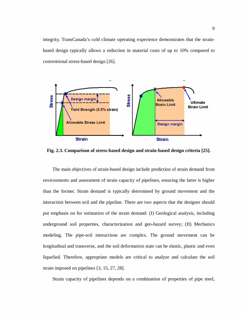
9

integrity. TransCanada’s cold climate operating experience demonstrates that the strain-

based design typically allows a reduction in material costs of up to 10% compared to

conventional stress-based design [26].

Fig. 2.3. Comparison of stress-based design and strain-based design criteria [25].

The main objectives of strain-based design include prediction of strain demand from

environments and assessment of strain capacity of pipelines, ensuring the latter is higher

than the former. Strain demand is typically determined by ground movement and the

interaction between soil and the pipeline. There are two aspects that the designer should

put emphasis on for estimation of the strain demand: (I) Geological analysis, including

underground soil properties, characterization and geo-hazard survey; (II) Mechanics

modeling. The pipe-soil interactions are complex. The ground movement can be

longitudinal and transverse, and the soil deformation state can be elastic, plastic and even

liquefied. Therefore, appropriate models are critical to analyze and calculate the soil

strain imposed on pipelines [3, 15, 27, 28].

Strain capacity of pipelines depends on a combination of properties of pipe steel,

10

welding, imperfection and geometries of pipelines. Development of pipe steels with a low

yield to tensile strength ratio (Y/T) and an adequate uniform elongation is capable of

increasing the strain capacity of pipelines. Higher strength steels may have a lower strain

capacity due to a reduced work hardening capacity, but they can significantly reduce the

strain demand because high strength steels are more resistant to soil deformation resulted

from ground movement. Welding has a significant effect on strain capacity of pipelines.

The strength and toughness of weld material and the heat affected zone (HAZ) are critical

to pipeline performance. An overmatch between the strength of the weld material and the

parent steel is usually required to ensure a safe design [29-30]. The presence of

imperfections, such as cracks, corrosion defects, welding flaws, etc., on pipe wall would

remarkably decrease the strain capacity of pipelines. In addition, an increase of pipe wall

thickness can reduce the strain demand and increase the strain capacity, but the steel

tonnage and cost will be excessive [20].

2.1.3 Requirements of mechanical properties for high strength steels

In order to accommodate the strain-based design in harsh environments, pipeline

steels should have a high strength, high deformability, excellent low-temperature

toughness and the field weldability [31-33]. The use of high strength pipeline steels such

as X80 and X100 steels can allow for considerable cost-effective designs, e.g., a

reduction of pipe wall thickness for a given pipe diameter and internal pressure, low pipe

transportation and pipe laying costs, a large diameter and a high operating pressure to

increase the transportation efficiency [34-39].

11

Fig. 2.4. Yielding types of pipeline steels and the influence on buckling [32].

Furthermore, the strength of pipeline steels has a great effect on the strain demand

and strain capacity. Generally, high strength steel pipelines have a high resistance to

ground movement, and the strain demand can be decreased with the increasing strength

of the steel. A lower yield to tensile strength ratio represents a greater strain hardening

capacity. A higher uniform elongation of steel can significantly increase the strain

capacity of pipelines. The yielding type of steels also influences the strain capacity. As

shown in Fig. 2.4, generally, the "round house in yielding" steel has a higher

deformability than the "Lüders elongation type" steel. Moreover, under the identical

pipeline geometry (D/t: diameter to wall thickness ratio), the "round house in yielding"

steel has a higher strain hardening capacity (n) and buckling strain than the “Lüders

elongation type” steel [9, 32, 34].

12

2.1.4 Metallurgical design and processing of high strength steels

In order to achieve a good balance of strength, deformability, toughness and

weldability for high strength steels, advanced micro-alloying, thermo-mechanical

controlled process (TMCP) techniques were introduced into metallurgical processing.

As shown in Fig. 2.5, the application of the thermal-mechanical rolling to replace hot

rolling and normalizing, combined with reduced carbon content and microalloying with

niobium (Nb) and vanadium (V) enables pipeline steels to reach grade X70 in 1970s. By

improving processing method, i.e., a thermo-mechanical rolling plus subsequent

accelerated cooling and further reduction of carbon content, the steel grade was increased

to X80. By adding elements such as molybdenum (Mo), copper (Cu) and nickel (Ni), etc.,

the steel grade was raised to X100 [40]. The very low carbon content of high strength

steels ensures an excellent toughness and the satisfactory field weldability. Addition of

boron (B) can further improve the low temperature toughness and strength. Mo is

important to enhance deformability of steel, but it is expensive. In order to decrease cost,

chromium (Cr) was used to replace Mo. Hara et al. [41] produced Mo-free X80 and X100

steels with the satisfactory deformability.

Through advanced TMCP techniques, an optimized microstructure can be achieved

with an excellent combination of strength and deformability of pipeline steels, i.e., a

dual-phase microstructure composed of a soft phase such as ferrite and a hard phase such

as bainite/martensite constituents, where the soft phase can provide sufficient

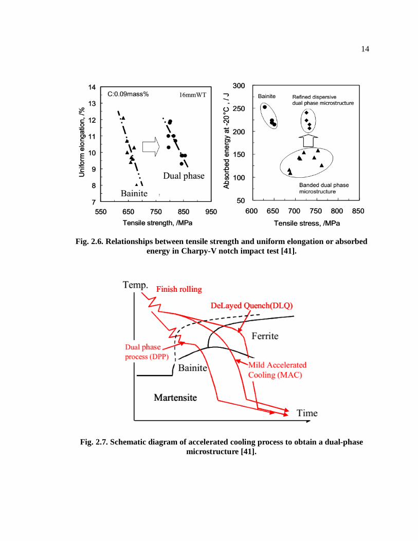
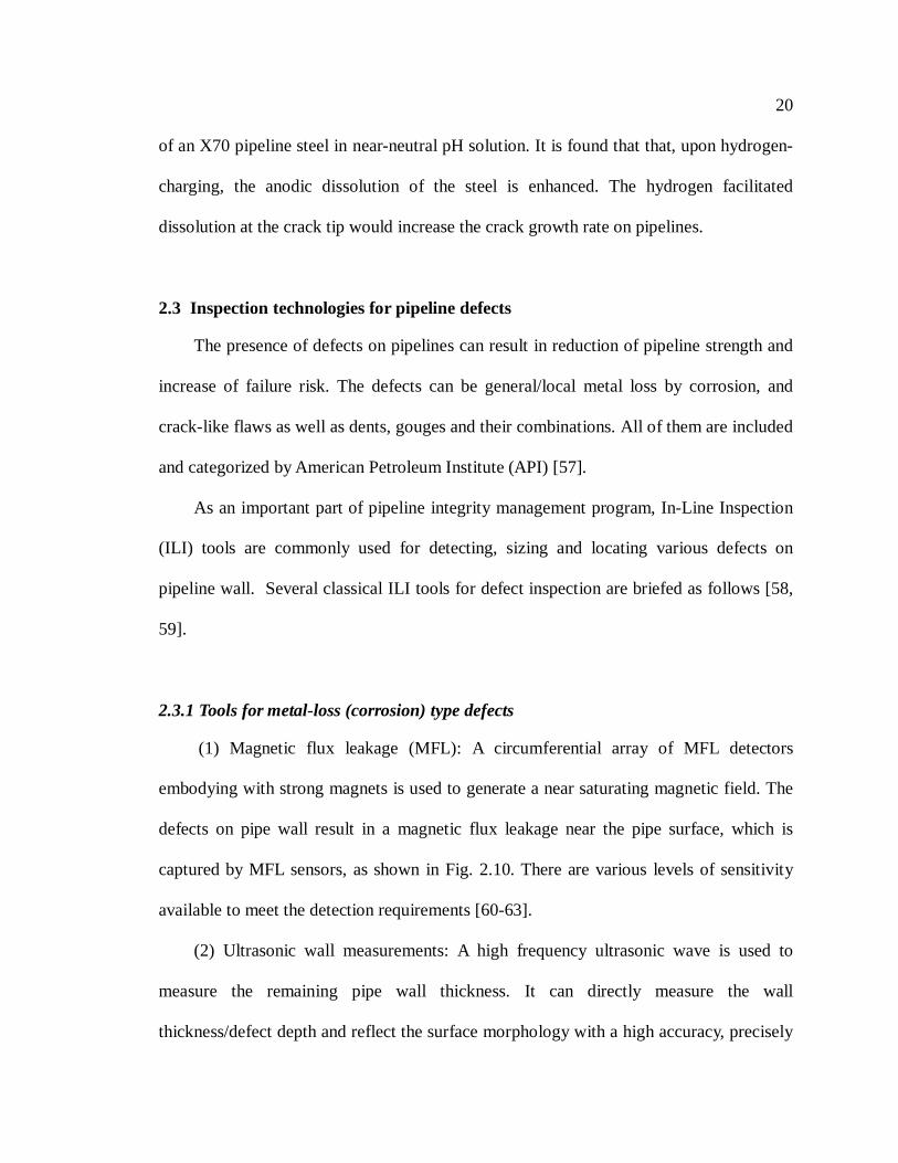
deformability and the hard phase can guarantee a high strength [31, 41]. As shown in Fig.

2.6, changing microstructure of pipeline steels from a bainite phase to a dual-phase can

improve both tensile strength and uniform elongation. A dual-phase microstructure is also

13

effective to decrease the Y/T ratio.

Fig. 2.5. Development of high strength pipeline steels [40].

Furthermore, as indicated in Fig. 2.6, a banded dual-phase microstructure is harmful

to low-temperature toughness because of occurrence of separation of the phases. A fine

dispersive dual-phase microstructure consists of a fine polygonal ferrite and dispersed

secondary hard phases such as bainite/martensite and martensite-austenite constituents,

and is effective for improving deformability and the low-temperature toughness of high

strength pipeline steels. Therefore, the TMCP process becomes critical to form the

desired dual-phase structure. As shown in Fig 2.7, there are three cooling processes, i.e.,

delayed quench process (DLQ), mild accelerated cooling (MAC) and dual-phase process

(DPP). The MAC process is preferred to obtain a fine dispersive dual-phase

microstructure, while the other two processes, DLQ and DPP, are likely to form the

banded microstructure [31, 41].

14

Fig. 2.6. Relationships between tensile strength and uniform elongation or absorbed energy in Charpy-V notch impact test [41].

Fig. 2.7. Schematic diagram of accelerated cooling process to obtain a dual-phase microstructure [41].

15

2.1.5 Effect of welding

The strain capacity of high strength pipeline steels is greatly affected by welding due

to the “bottleneck” of mechanical properties in weld seam, heat affected zone (HAZ) and

welding flaws. High strength steels are known to have potential to experience softening

in both weld seam and HAZ. Moreover, the weld region is susceptible to cracking due to

significant residual stress after welding. The irregular shape of weld seam can also

generate stress concentration. Therefore, pipelines can occur buckling adjacent to the

weld region when applied longitudinal compressive loads. The factors such as welding

residual stress, differences in metallurgical features and mechanical properties between

welding region and the parent steel, weld geometry and misalignment across the weld are

needed to take into consideration in the strain capacity assessment of pipeline [42, 43].

Wang [44] examined the specifications of girth weld for strain-based design of X100

steel pipeline, and found that the girth welds tend to be the weakest links in the pipeline

due to the existence of weld defects and changes of mechanical property resulted from

the welding thermal cycles.

2.2 Corrosion of pipelines

2.2.1 Overview of pipeline corrosion

Pipeline corrosion is a gradual destruction process of pipe steel due to

electrochemical reactions with the corrosive environment. There are many types of

corrosion based on their intrinsic mechanisms, such as pitting corrosion, galvanic

corrosion, crevice corrosion, and alternating current (AC) induced corrosion, etc. They all

result in reduction of the pipe wall thickness to form corrosion defects on either the

16

internal or external surface of pipelines.

Corrosion is one of the leading causes of pipeline failure. In Canada, 27% ruptures

of National Energy Board (NEB) regulated pipelines were caused by metal loss and 38%

caused by corrosion-related cracking, as shown in Fig. 2.8. Metal loss includes both

internal and external corrosion, and cracking includes hydrogen-induced and mechanical

damage delayed cracking, stress corrosion cracking, and corrosion fatigue [45]. Pipeline

failures usually cause serious consequences, e.g., huge economical and environmental

loss and even personal casualties. Therefore, corrosion prevention/mitigation and

assessment are of prime importance to pipeline industry.

Fig. 2.8. Canadian National Energy Board (NBE) regulated pipeline rupture causes between 1991 and 2009 [45]

17

2.2.2 General corrosion

General corrosion refers to the uniform reduction of wall thickness over the surface

of corroded pipelines, and is relatively easy to measure and predict. It represents only a

small fraction of corrosion-induced pipeline failures. General corrosion is usually

controlled by selecting suitable materials and applying protective coatings, cathodic

protection and corrosion inhibitors. However, the mechanical-electrochemical interaction

can make general corrosion become more complex.

Tang and Cheng [46] and Xue and Cheng [47] studied the effects of applied elastic

stress on corrosion of X70 and X80 pipeline steels, respectively. It was found that the

applied stress decreases the corrosion resistance and thus enhances the corrosion rate of

steels. Tang and Cheng’s results [46] further demonstrated that the stress-enhanced

corrosion rate is not significant under a relatively low stress (30%-60% of yield strength

of the steel). However, when the stress level reaches up to 80% of the yield strength, the

steel corrosion is increased obviously. Wang et al. [48] investigated the effect of strain on

corrosion of X80 steel in NaCl solution in both elastic and plastic deformation ranges.

The results showed that the applied strain can affect the steel corrosion. Particularly, in

plastic deformation, the multiplication, tangling and reaction of dislocations play an

important role in the enhanced corrosion activity of the steel.

2.2.3 Pitting corrosion

Pitting Corrosion is a localized corrosion confined to a point or a small area. The

driving power for pitting corrosion is the activation of a small area, which becomes

anodic while other vast area becomes cathodic, leading to localized corrosion. Pitting

18

corrosion is one of the most damaging forms of pipeline corrosion，as it can cause little

loss of steel with a small effect on the pipe surface, while it grows rapidly through the

pipe wall and is hard to be observed.

Pitting corrosion on pipelines is dependent on the metallurgical feature of the steel.

Alwaranbi [49] compared pitting corrosion of X80 and X100 steels, and found that X100

steel is more resistant to pitting corrosion in bicarbonate solution than X80 steel. This is

attributed to the higher microalloying content of Mo, Ni and Cu contained in X100 steel,

which can contribute to a higher stability of the steel.

Fig. 2.9. (a) SEM image of MnS inclusion; (b) stress field this inclusion for an applied stress of 350 MPa [50].

In environments experiencing ground movement, pipeline may be applied with

elastic and plastic strains. Since pitting corrosion is usually initiated at surface defects,

such as scratches, inclusions and dislocation emergence points, the mechanical

stress/strain condition of pipelines may affect the sensitivity of steel to pitting. Oltra and

Vignal [50] studied the role of stress on pitting initiation on a passivated steel and found

19

that the presence of inclusions has a strong effect on stress distribution on the steel

surface, and the pitting is enhanced by the stress gradient around the inclusion, as shown

in Fig. 2.9. Moreover, the enhancement of pitting corrosion would further increase the

non-uniform distribution of stress [51].

2.2.4 Stress corrosion cracking

Stress corrosion cracking (SCC) is resulted from the combined influence of tensile

stress and a corrosive environment. SCC can produce a marked loss of mechanical

strength with little metal loss. The stress corrosion cracks can cause a rapid mechanical

fracture and catastrophic failure of pipelines. Occurrence of SCC depends on three

conditions, i.e., a susceptible material, a corrosive environment and a sufficient tensile

stress. Pipelines have generally experienced two main forms of SCC, i.e., high pH and

near-neutral pH SCC. High pH SCC, usually resulting in an intergranular cracking,

generally occurs in the presence of a concentrated carbonate/bicarbonate environment

and at a pH greater than 9. The occurrence of near-neutral pH SCC is always associated

with an electrolyte characterized with anaerobic, dilute solutions with pH in the range of

6-7.5, and the crack is transgranular [52-54].

There is a common misunderstanding that the SCC of metals is related with their

strength levels. Actually there have been few general rules governing the influence of the

steel strength on the susceptibility of SCC. It has been demonstrated that pipeline SCC

can occur on a series of line pipe steels with various strength grades [55]. However, the

hydrogen permeation can increase the susceptibility of pipelines to SCC. Tang and Cheng

[56] studied the synergistic effect of hydrogen and stress on local dissolution at crack-tip

20

of an X70 pipeline steel in near-neutral pH solution. It is found that that, upon hydrogen-

charging, the anodic dissolution of the steel is enhanced. The hydrogen facilitated

dissolution at the crack tip would increase the crack growth rate on pipelines.

2.3 Inspection technologies for pipeline defects

The presence of defects on pipelines can result in reduction of pipeline strength and

increase of failure risk. The defects can be general/local metal loss by corrosion, and

crack-like flaws as well as dents, gouges and their combinations. All of them are included

and categorized by American Petroleum Institute (API) [57].

As an important part of pipeline integrity management program, In-Line Inspection

(ILI) tools are commonly used for detecting, sizing and locating various defects on

pipeline wall. Several classical ILI tools for defect inspection are briefed as follows [58,

59].

2.3.1 Tools for metal-loss (corrosion) type defects

(1) Magnetic flux leakage (MFL): A circumferential array of MFL detectors

embodying with strong magnets is used to generate a near saturating magnetic field. The

defects on pipe wall result in a magnetic flux leakage near the pipe surface, which is

captured by MFL sensors, as shown in Fig. 2.10. There are various levels of sensitivity

available to meet the detection requirements [60-63].

(2) Ultrasonic wall measurements: A high frequency ultrasonic wave is used to

measure the remaining pipe wall thickness. It can directly measure the wall

thickness/defect depth and reflect the surface morphology with a high accuracy, precisely

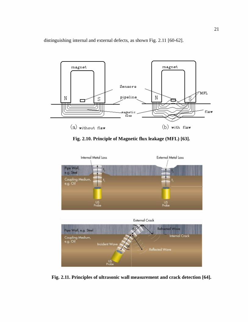
21

distinguishing internal and external defects, as shown Fig. 2.11 [60-62].

Fig. 2.10. Principle of Magnetic flux leakage (MFL) [63].

Fig. 2.11. Principles of ultrasonic wall measurement and crack detection [64].

22

2.3.2 Tools for crack-like defects

(1) Ultrasonic crack detection: An ultrasonic beam is emitted into pipe wall with a

certain angle relative to the longitudinal direction. If a crack is detected, the signal is

reflected back and detected. Since a “liquid coupling” is required between sensors and the

pipe wall, this tool is usually feasible for liquid pipelines. Some vendors have also

developed liquid filled wheels containing ultrasonic sensors for application in gas

pipelines, but these methods have limited inspection distances with ten miles or less [61-

64].

(2) Transverse MFL: The pipe wall is magnetized in circumferential direction to

detect longitudinal cracks. The principle of this tool is similar to that of standard MFL

tools, but with different imposed magnetic field directions.

Fig. 2.12. Principle of Electromagnetic Acoustic transducers (EMAT) [64].

23

(3) Electromagnetic acoustic transducers (EMAT): A coil is contained in a magnetic

field at the internal surface of pipelines. Alternating current placed through the coil

induces a current in the pipe wall, causing Lorentz forces, i.e., forces acting on moving

charges in magnetic fields, which in turn generate the ultrasound, as shown in Fig. 2.12.

This tool is developed for crack detection in gas pipelines without liquid coupling [65-67].

2.3.3 Tools for geometrical deformation

Geometry tools are used to obtain the geometric conditions of pipe wall. They are

aimed to detect the mechanical damage such as dents, buckles, wrinkles, etc., on

pipelines [60, 61].

(1) Caliper Pigs: A set of mechanical fingers or electromagnetic methods is used to

touch the internal surface of pipelines to detect dents or other types of deformations.

(2) Pipe Deformation Tools: Similar to caliper pigs, gyroscopes are combined to

provide the clock position of the dents or deformations on pipelines. This technique can

also provide pipe bend information.

(3) Mapping Tools: While this technique can be applied as a single inspection tool,

units are often in conjunction with other tools (such as MFL) to provide global

positioning system (GPS) correlated mapping of the pipeline and other physical location

information, such as valves and fittings [60, 61, 68].

Particularly, a novel inspection technology, i.e., pipeline laser imaging and

metrology using laser optical sensors, has been developed recently. This technology can

operate with a high speed laser scanning, and produce a virtual reality 3D imaging of

internal surface of pipe wall. It can detect any defects due to corrosion, erosion and any

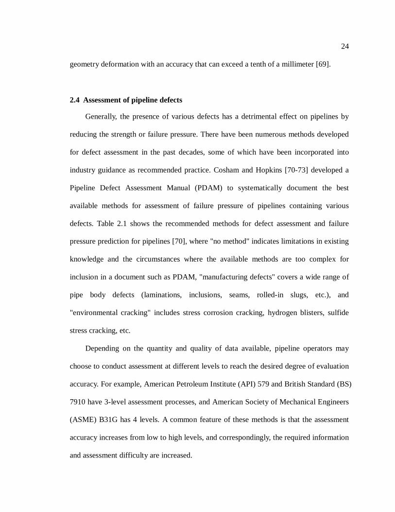
24

geometry deformation with an accuracy that can exceed a tenth of a millimeter [69].

2.4 Assessment of pipeline defects

Generally, the presence of various defects has a detrimental effect on pipelines by

reducing the strength or failure pressure. There have been numerous methods developed

for defect assessment in the past decades, some of which have been incorporated into

industry guidance as recommended practice. Cosham and Hopkins [70-73] developed a

Pipeline Defect Assessment Manual (PDAM) to systematically document the best

available methods for assessment of failure pressure of pipelines containing various

defects. Table 2.1 shows the recommended methods for defect assessment and failure

pressure prediction for pipelines [70], where "no method" indicates limitations in existing

knowledge and the circumstances where the available methods are too complex for

inclusion in a document such as PDAM, "manufacturing defects" covers a wide range of

pipe body defects (laminations, inclusions, seams, rolled-in slugs, etc.), and

"environmental cracking" includes stress corrosion cracking, hydrogen blisters, sulfide

stress cracking, etc.

Depending on the quantity and quality of data available, pipeline operators may

choose to conduct assessment at different levels to reach the desired degree of evaluation

accuracy. For example, American Petroleum Institute (API) 579 and British Standard (BS)

7910 have 3-level assessment processes, and American Society of Mechanical Engineers

(ASME) B31G has 4 levels. A common feature of these methods is that the assessment

accuracy increases from low to high levels, and correspondingly, the required information

and assessment difficulty are increased.

25

Table 2.1. Recommended methods for defect assessment on pipelines [70].

Built upon the industry standards and codes, researchers developed more detailed

assessment processes with increased levels or stages and improved accuracy. For example,

Alexander [74] developed a 5-level Engineering-Based Integrity Management Program

(EB-IMP) for evaluation of pipeline integrity based on API 579’s 3-level assessment

26

process, with details shown in Fig. 2.13.

Fig. 2.13. Flowchart showing elements of the EB-IMP process [74].

In API 579, fitness-for-service (FFS) 3-level assessment process includes [57]:

(1) Level 1: Conservative screening criteria that can be utilized with a minimum

amount of inspection or component information are provided. The Level 1 assessment

can be performed either by plant inspection or engineering personnel.

(2) Level 2: A more detailed evaluation is provided to produce results that are more

precise than those from the Level 1 assessment. In a Level 2 assessment, inspection

information similar to that required for Level 1 assessment is needed; however, more

detailed calculations are used in the evaluation. Level 2 assessment would typically be

conducted by plant engineers, or engineering specialists, who are experienced and

knowledgeable in performing FFS assessments.

(3) Level 3: The most detailed evaluation is provided to produce results that are

27

more precise than those from Level 2 assessment. In a Level 3 assessment the most

detailed inspection and component information is typically required, and the

recommended analysis is based on numerical techniques such as the finite element

method or experimental techniques when appropriate. A Level 3 assessment is primarily

intended for use by engineering specialists experienced and knowledgeable in performing

FFS assessments.

Alexander [74] further refined the "Level 3" in API 579 and listed a Level 4

assessment in "EB-IMP" process by performing an experimental testing program to

validate the results of engineering and finite element analysis. Finally, a repair procedure

is proposed to remediate the integrity on pipeline as "Level 5" assessment. As seen in Fig.

2.13, the testing approach in "Level 4" is extremely powerful and provides pipeline

operators with means for quantifying integrity concerns that not possible using the Levels

1, 2 or 3 assessments. The Level 5 approach is used to develop a repair procedure to meet

the specific needs of situations. The design for repair is typically evaluated by numerical

modeling and experimental testing to ensure the reliability before field application.

2.5 Prediction of failure pressure of pipelines containing defects

2.5.1 Overview of defect assessment models

Numerous models have been developed to calculate failure pressure of pipelines and

to estimate the remaining strength of the line pipe steel. These include:

(1) NG-18 [75];

(2) ASME B31G [14];

(3) Modified B31G (or RSTRENG-0.85) [76, 77]

28

(4) RSTRENG [78]

(5) SHELL-92 [79]

(6) DNV-RP-F101 [15]

All models were developed based on extensive numerical calculations and

experimental full-scale burst tests. They consider primarily the longitudinal extent of

defect area and the internal pressure. In particular, the NG-18 model is the base of other

models.

According to the NG-18 model,

⋅−

−=

MAA

AA

DtP flowF 11

12

0

0σ (2.1)

4

42

)()2/(54.0)2/(51.21

DtL

DtLM −+= (2.2)

where PF is the estimated failure pressure of pipeline, flowσ is flow stress ( flowσ =1.1

SMYS, and SMYS is specified minimum yield strength of pipe steel), D is outer diameter

of the pipe, t is the pipe wall thickness, d is depth of defect, A0 = L t, A is the projected

area of defect, L is length of defect, and M is a Folias bulging factor, accounting for the

effect of stress concentration at defect.

By modifying factors contained in the NG-18 equation, such as flow stress flowσ ,

bulging factor M, and defect’s shape factor A/A0, some other models including ASME

B31G, Modified B31G, etc. were developed with a higher accuracy to calculate the failure

29

pressure of corroded pipelines. Table 2.2 shows the comparison of the listed six models,

where flow stress flowσ can be interpreted as the failure stress of pipelines in the absence

of defects. It varies from 1.1×SMYS to SMYS+69 MPa, 0.9×SMTS and SMTS, where

SMTS is the specified minimum tensile strength of pipe steel.

Fig. 2.14, Dimensions of corrosion defect [15].

The projected corrosion area A can be varied from dL, 2/3×dL and 0.85×dL to the

"exact" area, as shown in Fig. 2.14. The defect is orientated and spaced on pipelines in a

random manner with an irregular 3D profile. However, all the assessment models, except

the "RSTRENG" model which needs an exact defect area, make a simple approximation

of the defect area based on the maximum depth d and length L. The most conservative

approximation is a rectangular shape with area of "A = dL", like the NG-18, Shell-92 and

DNV-RP-F101 models. The ASME B31G model assumes a parabolic shape (2/3×dL) and

modified B31G uses "0.85×dL" shape, which is between rectangular and parabolic shapes.

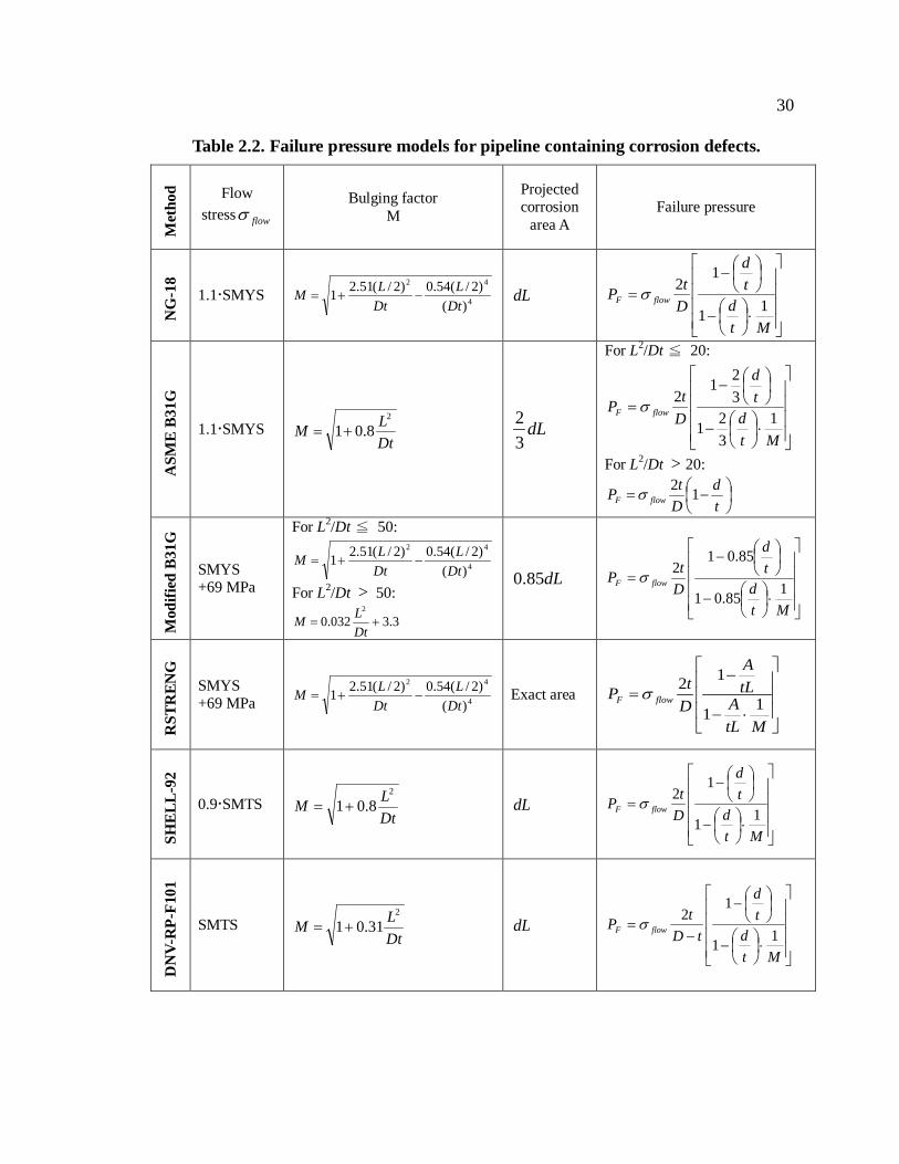
30

Table 2.2. Failure pressure models for pipeline containing corrosion defects. M

etho

d Flow stress flowσ

Bulging factor M

Projected corrosion

area A Failure pressure

NG

-18

1.1SMYS 4

42

)()2/(54.0)2/(51.21

DtL

DtLM −+= dL

⋅

−

−

=

Mtd

td

DtP flowF 11

12σ

ASM

E B3

1G

1.1SMYS DtLM

2

8.01+= dL32

For L2/Dt ≦ 20:

⋅

−

−

=

Mtd

td

DtP flowF 1

321

321

2σ

For L2/Dt > 20:

−=

td

DtP flowF 12σ

Mod

ified

B31

G

SMYS +69 MPa

For L2/Dt ≦ 50:

4

42

)()2/(54.0)2/(51.21

DtL

DtLM −+=

For L2/Dt > 50:

3.3032.02

+=DtLM

dL85.0

⋅

−

−

=

Mtd

td

DtP flowF 185.01

85.012σ

RST

REN

G

SMYS +69 MPa 4

42

)()2/(54.0)2/(51.21

DtL

DtLM −+= Exact area

⋅−

−=

MtLA

tLA

DtP flowF 11

12σ

SHEL

L-92

0.9SMTS DtLM

2

8.01+= dL

⋅

−

−

=

Mtd

td

DtP flowF 11

12σ

DN

V-R

P-F1

01

SMTS DtLM

2

31.01+= dL

⋅

−

−

−=

Mtd

td

tDtP flowF 11

12σ

31

2.5.2 Limitations of the present assessment models

The abovementioned models for defect assessment on pipelines are semi-empirical

equations which are used to calculate the failure pressure of corroded pipelines. Pipelines

experiencing ground movement may suffer from appreciable strains. These models are

not able to estimate the effect of soil strain on the failure pressure of pipelines.

Furthermore, the present models were derived based on experimental tests on low

grades of line pipe steel. For example, the ASME B31G model was derived and validated

through a large number of full-scale tests conducted on X52 and X65 steels, and the

DNV-RP-F101 model was verified by 138 burst tests performed on steels from X42 to

X65 grades. Thus, these models are not applicable for high grades of pipeline steel, e.g.,

X80 and X100 steels.

2.6 Prediction of remaining service life of pipelines containing defects

Prediction of remaining service life of corroded pipelines is primarily dependent on

comparison between failure pressure (PF) and internal operating pressure (Pi). When the

former is less than the latter i.e., 0≤−= iF PPz , the pipeline will fail. In the long-term

service, the failure pressure of pipelines depends not only on the mechanical properties of

the pipe steel and the defect geometry, but also on the growth rate of defect usually

driven by local corrosion reaction. Take the DNV-RP-F101 model as an example, both

the defect length and depth are a function of time (T).The model then becomes [80-82]:

32

⋅

−

−

−=

MtTd

tTd

tDtSMTSPF 1)(1

)(12 (2.3)

DtTLM

2))((31.01+= (2.4)

iF PPz −= (2.5)

When z=0 at a certain elapsed time (T), the value T is the predicted remaining life of the

corroded pipeline.

To date, a linear defect growth model with a constant corrosion rate at defect has

been extensively employed based on simplifying calculations. A typical expression of the

defect depth and length as a function of time is [81, 83-85]:

)()( 00 TTVdTd d −+= (2.6)

)()( 00 TTVLTL L −+= (2.7)

where dV is the growth rate in depth direction, LV is the growth rate in length direction,

and 0d and 0L are the initial depth and length at time 0T , respectively. Combine Eqs. 2.6

and 2.7 with Eqs. 2.3-2.5, the remaining life of pipelines containing corrosion defects can

be estimated. However, the prediction of the growth rate of a corrosion defect in this way

is not representative of the reality. The defect growth may be accelerated or reduced with

elapsed time. In some environments, the formation of corrosion product layer can also

affect the growth rate, which has been found to be a high value initially and then decrease

33

gradually [86]. Furthermore, variations of the defect geometry, corrosive environments,

temperature and the presence of mechanical stress/strain also affect the growth rate of

defects [56, 87]. An accurate prediction of the defect growth is up to a complete, reliable

simulation of the effects of all relevant factors mentioned above.

34

Chapter Three: Research methodology

3.1 Materials and solutions

Specimens used in this work were cut from a sheet of X100 steel pipe, with a

chemical composition shown in Table 3.1. The specimens were machined into four types

of geometry, as shown in Fig. 3.1, where (a) and (b) show flat-plate specimens for micro-

electrochemical impedance and current density measurements, (c) shows a rod-type

specimen for tensile tests and conventional macro-electrochemical measurements, and (d)

shows a rectangular specimen with artificial defects created for local potential and current

density measurements. The red-marked lines on specimens in Figs. 3.1a, b and d are the

designated micro-probe scanning paths for micro-electrochemical measurements.

Prior to test, the specimen was ground sequentially up to 1000 grit silicon carbide

paper, and then rinsed with deionized water and degreased in acetone.

The test solution was a near-neutral pH, diluted bicarbonate solution, called NS4

solution, which has been used widely to simulate the electrolyte trapped under disbonded

coating [88]. The solution contained 0.483 g/L NaHCO3, 0.122 g/L KCl, 0.181 g/L

CaCl2.H2O and 0.131 g/L MgSO4.7H2O, made from analytic grade reagents and ultra-

pure water (18 MΩcm in resistivity). Prior to each test, the solution was purged with 5%

CO2 balanced with N2 gas for 1 h to achieve an anaerobic and near-neutral pH condition

(pH=6.8). The gas flow was maintained throughout the test.

All the tests were performed at ambient temperature (~22oC).

35

Table 3.1. Chemical composition of X100 steel (wt.%)

C Mn S Si P Ni Cr Mo V Cu Al

0.07 1.76 0.005 0.1 0.018 0.154 0.016 0.2 0.005 0.243 0.027

(b)

(a)

(c)

36

Fig. 3.1. Schematic diagrams of various types of specimens used in this work: (a) and (b) flat-plate specimens; (c) rod specimen; (d) rectangular specimen containing

artificial defects.

3.2 Mechanical tensile testing

Mechanical tensile testing was performed on the rod-type specimen (Fig. 3.1c)

through a Bose Electroforce dynamic materials test system. Based on American Society

for Testing and Materials (ASTM) E8/E8M-09 standard [89], a strain rate of 1×10-4 /s

was applied to obtain stress-strain curve of the steel.

The specimen was plastically deformed under various pre-strains, i.e., 0.985%,

2.262% and 3.918%, determined from the measured stress-strain curve. The strain at

yielding of the steel was approximately 0.388%. Prior to test, the specimen was pre-

loaded at 300 N in order to avoid any misreading in elongation or time to failure. Load-

(d)

37

elongation data was recorded during test. After test, the diameter of the fracture surface

of the specimen was measured to calculate the percent reduction-in-area (RA%).

3.3 Conventional macro-electrochemical measurements

Conventional electrochemical measurements were performed on the rod-type steel

specimen while it is in tensile testing through a Solatron 1280C electrochemical system.

The experimental setup is shown in Fig. 3.2, where the rod-type steel specimen that was

as a working electrode (WE) was installed in a three electrode environmental cell, with a

saturated calomel electrode (SCE) as reference electrode (RE) and a carbon rod as

counter electrode (CE).

During electrochemical measurements, there are two types of mechanical

deformation applied on specimen WE-1 in Fig. 3.2, i.e., elastic and plastic deformations,

respectively. In elastic deformation, the tensile and compressive stresses that were below

the yield stress of ~803 MPa of the steel were applied on the specimen at the desired

values, i.e., 0, 200, 400 and 600 MPa, respectively, by adjusting the output load of the

machine with a loading rate of 1000 N/s (31.57 MPa/s). In plastic deformation, a tensile

strain rate of 1×10-4 /s was applied on the specimen to reach the specific strain level.

Two types of potential measurements were conducted during tensile testing of the

steel specimen, i.e., open circuit potential of specimen WE-1 relative to SCE and the

coupling potential of the coupled specimens WE-1 and WE-2 relative to RE, where WE-2

is an identical steel specimen, but not stressed. Moreover, the current flowing between

WE-1 and WE-2 was measured through a zero resistance ammeter (ZRA).

38

The electrochemical impedance spectroscopy (EIS) of the steel specimen WE-1 was

measured at corrosion potential under various stress or strain levels. Before EIS

measurement, corrosion potential of the steel was recorded until a steady state value was

achieved. For EIS measurements, an AC disturbance signal of 10 mV was applied on the

steel specimen, and the measuring frequency ranged from 20000 Hz to 0.01 Hz.

Potentiodynamic polarization curve was measured on specimen WE-1 after steady-

state corrosion potential was achieved upon immersing in NS4 solution for 1 h. The

potential scanning rate was 0.3 mV/s, and potential polarization started at -0.9 V(SCE)

and ended at -0.6 V(SCE).

Fig. 3.2. Schematic diagram of the experimental setup for various macro-electrochemical measurements on X100 steel specimen.

39

3.4 Micro-electrochemical measurements

The localized electrochemical impedance spectroscopy (LEIS) and scanning

vibrating electrode technique (SVET) measurements were performed on the flat steel

specimen through a PAR Model 370 scanning electrochemical workstation. As shown in

Fig. 3.3, the M370 system was comprised of a scanning microprobe with a 10 microns tip,

a scanning control unit, a M236A potentiostat, a M5210 lock-in amplifier and a video

camera system. A SCE was used as reference electrode and a platinum wire as counter

electrode. The specimen was stressed through a compressive spring installing at one side

of the electrochemical cell. The applied tensile force was 2000 N for the flat-plate

specimen shown in Fig. 3.1a, and 2750 N on the specimen shown in Fig. 3.1b. The

resulting stress levels were calculated from the spring’s elastic coefficient and the change

in length. The stress and strain distributions along the red-colored line on the specimen

were determined by finite element analysis, with the details described in Chapters 4 and 5.

During LEIS measurements, the distance between the micro-tip and the specimen

surface was 200 µm. An AC disturbance signal of 10 mV was applied on the electrode at

its corrosion potential, and the measuring frequency was fixed at 0.5 Hz. The microprobe

was set in a linear scan mode along the path marked as red in Figs. 3.1a and 3.1b.

The current density was measured on the flat-plate specimen (Fig. 3.1b) and the

rectangular specimen (Fig. 3.1d) through the SVET. The vibrating amplitude of the

micro-electrode was 30 µm and the vibrating frequency was 300 Hz. The distance

between microprobe and the electrode surface was 200 µm. The microprobe was also set

in a linear scan mode along the path marked as red in Figs. 3.1b and 3.1d.

40

Fig. 3.3. Schematic diagram of the experimental setup of micro-electrochemical measurements on the steel specimen through the M370 scanning electrochemical

workstation.

Fig. 3.4. Schematic diagram of the home-made potential microprobe for potential measurement at defects.

Potentiometer

Insulating layer Thickness=0.05 mm

Platinum wire Diameter=0.38 mm

3-axis motion

Steel coupon

Local potential measurement probe

Rigid holder

Z

Y X

Exposed probe tip

CP

CE

41

0 400 800 1200 1600 2000 24000.10

0.15

0.20

0.25

0.30

0.35

0.40

Pote

ntia

l (V,

SCE

)

Time (s)

Fig. 3.5. Time dependence of the open-circuit potential of the home-made potential microprobe vs. SCE in NS4 solution.

The distribution of potential inside defects that are present on the rectangular

specimen (Fig. 3.1d) was measured using a home-made microprobe, as illustrated in Fig.

3.4. It was made of a platinum wire with a diameter of 0.48 mm. The surface of the

platinum wire was coated with a 0.05 mm thick methyl 2-cyanoacrylate electric

insulating layer, leaving a tip exposed to solution. To calibrate the platinum wire

microprobe for potential measurements, its open-circuit potential vs. SCE was measured

in NS4 solution and the result is shown in Fig. 3.5. Apparently, the microprobe showed a

high stability in the solution. With help of a 3-axis motion platform equipped in the M370

scanning electrochemical workstation, the microprobe was able to either move over the

42

surface of the steel electrode or penetrate into defects. The scanning path of the

microprobe inside defect was along its central line from top to bottom with a total depth

of 7.5 mm, as marked in red in Fig. 3.1d. Measurement of potential on the electrode

surface was along the horizontal central line (from left to right with a total length of 55

mm) marked in red in Fig. 3.1d. The distance between the microprobe and the steel

electrode was controlled precisely at 200 µm.

3.5 Surface characterization

The morphology of corrosion scale formed on the steel specimen after test was

characterized by a scanning electron microscopy (SEM) (Model Philips XL 30).

43

Chapter Four: Pipeline corrosion under mechanical-electrochemical interaction - Elastic deformation

Corrosion of pipelines that are made of various grades of steel, including X65, X70

and X80 steels, in environments that are relevant to the pipeline operation have been

studied comprehensively in Cheng's CorrPIPE group [46, 47, 56, 87, 90-97]. It has been

demonstrated that an applied stress enhances anodic dissolution of pipeline steels.

Moreover, the local stress concentration developed at various discontinuities, such as

cracks, would favor the hydrogen accumulation, contributing to an accelerated localized

corrosion and crack propagation [87, 98, 99].

Pipelines made of high-strength steels, such as X100 steel, would experience

complex stress/strain conditions in environments with significant ground movement, such

as the Arctic and sub-Arctic areas in North America. In addition to hoop stress resulted

from the internal pressure, a longitudinal strain is induced by soil movement and exerts

on the pipe steel. It is expected that the mechanical-electrochemical interaction plays an

essential role in pipeline corrosion. By now, there have been a number of researches,

including those conducted in Cheng’s CorrPIPE group, to understand this interaction, but

at a qualitative level. Both the mechanism and quantitative treatments have been lacking.

In this chapter, corrosion of X100 pipeline steel that is under elastic deformation

was investigated by LEIS, corrosion potential and conventional electrochemical

impedance measurements (EIS) measurements and surface analysis techniques as well as

finite element analysis. Various stressing conditions, including stress intensity,

tensile/compressive nature and static/dynamic loading, were applied on the steel

44

specimen, and the effect on the steel corrosion was determined. A theoretical model was

proposed to illustrate pipeline corrosion under the mechanical-electrochemical interaction

under the elastic deformation condition.

4.1 Results

4.1.1 Mechanical testing

0.00 0.02 0.04 0.06 0.08 0.10 0.12 0.14 0.160

100

200

300

400

500

600

700

800

900

1000

Stre

ss (M

Pa)

Strain

Fig. 4.1. Engineering stress-strain curve of X100 steel specimen measured in air.

Fig. 4.1 shows the engineering stress-strain curve measured on the rod specimen

(Fig. 3.1c) under a tensile strain of 1×10-4 /s in air. It is seen that the engineering yield

stress and ultimate tensile stress (UTS) are about 803 MPa and 860 MPa, respectively,

and the engineering failure strain is about 0.14.

45

4.1.2 LEIS measurements

Fig. 4.2 shows the linear LEIS results measured on the flat steel specimen shown in

Fig. 3.1a after 2 days of immersion in NS4 solution under different stressing conditions,

i.e., (a) no load applied on the specimen; (b) 2000 N force applied before immersion; and

(c) 2000 N force applied after immersion. It is seen that the impedance values measured

under conditions (a) and (b) are quite similar, and fluctuate around 760 Ω along the

scanning line. Apparently, a tensile force of 2000 N applied before immersion does not

affect corrosion of the steel. However, if a tensile force of 2000 N is applied after 2 days

of immersion in NS4 solution, i.e., the condition (c), the impedance decreases

continuously from the wide side of the specimen to the narrow side, indicating that

corrosion of the steel increases following the scanning direction since the impedance is

inversely proportion to corrosion rate.

4.1.3 Corrosion potential and EIS measurements

Fig. 4.3 shows the corrosion potential of the X100 steel rod tensile specimen (Fig.

3.1c) in NS4 solution during dynamic loadings (loading applied at the 300th s) from 0 to

tensile 600 MPa or compressive 600 MPa, respectively. It is seen that the corrosion

potential jumps upon the application of the tensile force at 300 s, and then recovers

gradually to its initial value although the specimen is still under the tensile loading.

However, there is no apparent change of corrosion potential when the compressive

loading is applied on the specimen.

46

Fig. 4.2. LEIS line scanning measurements on the flat steel specimen (Fig. 3.1a) after 2 days of immersion in NS4 solution under different test conditions: (a) no load

applied on the specimen; (b) 2000 N force applied before immersion; and (c) 2000 N force applied after immersion.

Fig. 4.3. Corrosion potential of X100 steel rod tensile specimen (Fig. 3.1c) in NS4 solution during dynamic loadings (loading applied at 300 s) from 0 to tensile-600

MPa or compressive-600 MPa, respectively.

(a)

(b)

(c)

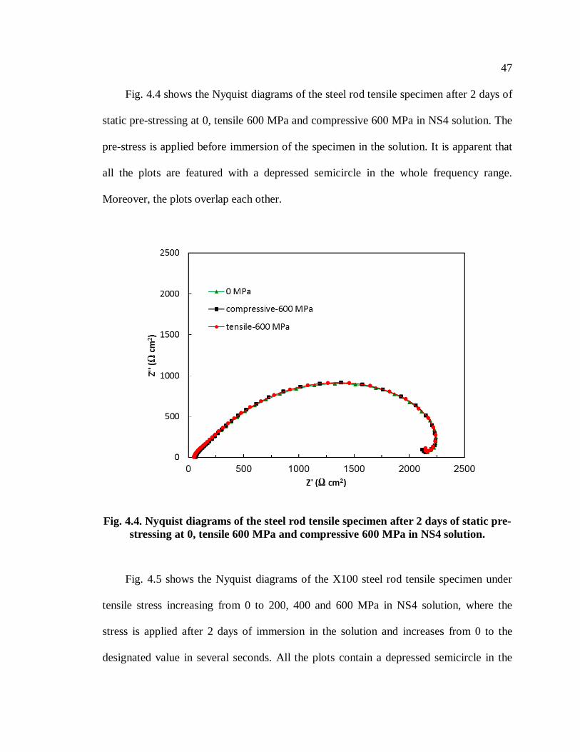
47

Fig. 4.4 shows the Nyquist diagrams of the steel rod tensile specimen after 2 days of

static pre-stressing at 0, tensile 600 MPa and compressive 600 MPa in NS4 solution. The

pre-stress is applied before immersion of the specimen in the solution. It is apparent that

all the plots are featured with a depressed semicircle in the whole frequency range.

Moreover, the plots overlap each other.

Fig. 4.4. Nyquist diagrams of the steel rod tensile specimen after 2 days of static pre-stressing at 0, tensile 600 MPa and compressive 600 MPa in NS4 solution.

Fig. 4.5 shows the Nyquist diagrams of the X100 steel rod tensile specimen under

tensile stress increasing from 0 to 200, 400 and 600 MPa in NS4 solution, where the

stress is applied after 2 days of immersion in the solution and increases from 0 to the

designated value in several seconds. All the plots contain a depressed semicircle in the

48

whole frequency range. Moreover, the semicircle size decreases with the increasing

tensile stress.

Fig. 4.6 shows the Nyquist diagrams of the steel specimen under compressive stress

increasing from 0 to 200, 400, 600 MPa in NS4 solution. It is clear that all the plots are

featured with a depressed semicircle in the whole frequency range, and the semicircle

size increases slightly with the increasing compressive stress.

Fig. 4.5. Nyquist diagrams of X100 steel specimen under dynamic tensile stress

increasing from 0 to 200, 400 and 600 MPa in NS4 solution, where the stress was applied after 2 days of immersion in the solution and increased from 0 to the

designated value in several seconds.

49

Fig. 4.6. Nyquist diagrams of X100 steel under compressive stress increasing from 0

to 200, 400, 600 MPa in NS4 solution.

Fig. 4.7. The von Mises stress distribution of the flat specimen under a tensile force

of 2000 N.

50

4.1.4 FEA of stress and strain distributions on the steel specimens

Fig. 4.7 shows the von Mises stress distribution on the flat specimen (Fig. 3.1.a)

under a tensile force of 2000 N. It is seen that the von Mises stress on the specimen is

below the 803 MPa yield strength of X100 steel. This indicates that the specimen is under

an elastic deformation. Moreover, there is a stress concentration at the narrow side.

Fig. 4.8 shows the von Mises stress and strain distributions along the red-marked

line on the flat specimen (Fig. 3.1a). It is seen that both the von Mises stress and strain

increase from the wide side to the narrow side of the specimen. Particularly, the von

Mises increases from 264 MPa to 582 MPa, and the strain changes from 0.13 % to 0.29%.

Fig. 4.8. The von Mises stress and strain distribution along the red-marked line on

the flat specimen.

51

Fig. 4.9. von Mises stress distribution on the rod specimen under tensile or

compressive force of 19000 N.

Fig. 4.9 shows the von Mises stress distribution on the rod tensile specimen under

tensile or compressive force of 19000 N. It is seen that there is a uniform stress of 600

MPa distributing on the testing section of the specimen.

4.1.5 Surface characterization

Fig. 4.10 shows the SEM view of corrosion product formed on the surface of the

steel specimen after tensile testing in NS4 solution. It is seen that the corrosion product is

featured with a porous structure, depositing on the steel surface.

52

Fig. 4.10. SEM view of corrosion product formed on the surface of X100 steel specimen after tensile test in NS4 solution.

4.2 Discussion

4.2.1 Electrochemical corrosion behavior of X100 steel in NS4 solution

The electrochemical anodic and cathodic reactions of X100 steel in the

deoxygenated, near-neutral pH NS4 solution are dissolution of Fe and the hydrogen

evolution, respectively [54, 92, 94, 103, 104]:

Anodic reaction: Fe → Fe2+ + 2e (4.1)

Cathodic reaction: 2H2O + 2e → H2 + 2OH- (4.2)

In CO2-containing environments, a layer of porous corrosion product forms and

deposits on the steel surface, as shown in Fig. 4.10, by:

53

Fe2+ + HCO3- → FeCO3 + H+ (4.3)

The depressed semicircle in the EIS plots shown in Figs. 4.4-4.6 is attributed to the

interfacial electrode reaction of the scale-covered steel electrode in the solution. It is

usually fitted with an electrochemical equivalent circuit of a parallel connection of

charge-transfer resistance (Rct) and double-charge layer capacitance (Cdl), which is

connected in series with a solution resistance (Rs). The electrochemical parameters

obtained by fitting the experimental data are shown in Tables 4.1 and 4.2. It is seen that

the value of Rct decreases with the increasing tensile stress, but increases slightly with the

applied compressive stress. Since the charge-transfer resistance is inversely proportional

to corrosion rate, the tensile and compressive stresses increases and decreases the

corrosion rate of the steel, respectively.

Table 4.1. Electrochemical parameters fitted from EIS data measured under various tensile stresses

Tensile stress (MPa) 0 200 400 600 Rct (Ω cm2) 2843 2835 2793 2742

Cdl (µF/cm2) 246.1 244.9 259.9 252.6

Table 4.2. Electrochemical parameters fitted from EIS data measured under various compressive stresses

Compressive stress (MPa) 0 200 400 600

Rct (Ω cm2) 2463 2468 2501 2535

Cdl (µF/cm2) 285.9 289.1 295.0 296.8

54

4.2.2 Effect of static elastic stress/strain on corrosion of the steel

The present work demonstrates that the applied elastic stress may affect corrosion of

the steel. This effect is attributed to two aspects as analyzed below.

The first aspect is the electrochemical thermodynamic activity of the steel. A theory

of “mechanical-electrochemical interactions” was initially developed by Gutman [105],

who proposed that the corrosion activity of a metal is affected by external pressure,

which is expressed by the change of equilibrium electrochemical potential 0ϕ∆ :

zFPVm∆

−=∆ 0ϕ (4.4)

where P∆ is the excess pressure (Pa), is the molar volume of the substrate (m3/mol), z is

the charge number, and F is Faraday’s constant (C/mol). Therefore, an external pressure

( P∆ >0) can decrease the equilibrium potential of steel, resulting in an increase of the

electrochemical thermodynamic activity [48, 106].

In this work, a uniaxial stress (σ) is applied on the steel electrode (rod tensile

specimen), and P∆ , as the hydrostatic pressure, equals to 1/3 of the applied stress [105].

Take the relevant parameters and the maximum uniaxial stress of 600 MPa into Eq. (4.4),

it is calculated that the theoretical change of the equilibrium electrochemical potential is

0ϕ∆ =7.4 mV. Moreover, the measured steady-state potential in Fig. 4.3 is a compromise

potential of both anodic and cathodic reactions. Its change can be less than the theoretical

equilibrium potential change of 7.4 mV.

55

According to the mechanical-electrochemical effect on corrosion of steels [105],

there would be several millivolts of potential difference between a stress-free steel

electrode and a pre-stressed electrode. The corrosion activity of the latter is slightly

higher than the former, which would influence the formation of corrosion scale on the

steel surface after 2 days of immersion in NS4 solution. The pre-stressed specimen may

have a thicker or more compact scale, leading to an “offsetting effect” on the enhanced

corrosion activity resulted from pre-stressing. As a consequence, the effect of static

elastic stress on the steel corrosion is not obvious, and not detected in this work. Thus, an

application of static elastic stress with 600 MPa has very limited effect on corrosion of

X100 steel after 2 days of immersion, as shown in Fig. 4.4.

The second aspect concerns the effect of the mechanical strain induced by external

loading on corrosion scale formed on the steel surface. Generally, the corrosion scale

formed on the steel surface has different mechanical properties, such as strength and

ductility, from the steel substrate. Whether the corrosion scale breaks under application of

a tensile stress/strain depends on if the critical failure strain of the scale is exceeded.

Assume that the corrosion scale is macroscopically uniform and continuous, the critical

failure strain, εcrit, of corrosion scale can be calculated by [107]:

5.0

22

=

EhfAcrit πγε (4.5)

where γ is the surface fracture energy (J/m2), A is a numerical factor, f is a constant

between 0 and 1, and h is the thickness of corrosion scale.

56

In this work, the corrosion scale formed on X100 steel in NS4 solution is primary

iron carbonate, which has an estimated theoretical Young's modulus (E) of 150 GPa

[108]. Gao et al. [109] measured E of the iron carbonate scale by a nano-indentation

method, and got the value of about 110 GPa. The surface fracture energy, γ , of iron

carbonate is approximately 3 J/m2. The values of A and f are assumed as 1 and 0.1,

respectively [110]. The average thickness of the iron carbonate scale deposited on X100

steel after 2 days of immersion is roughly 10 µm measured by a magnetic induction

method. Take these parameter to Eq. 4.5, the critical failure strain of the corrosion scale

in this work is calculated to be 0.00357 ~ 0.00417, which is higher than the maximum

strain of 0.0029 under the applied stress of 582 MPa, as seen in Figs. 4.7 and 4.8. Thus,

the corrosion scale formed on the steel surface will not fracture under the applied loading.

Although the corrosion scale is not fractured under the applied elastic strain, its

porosity can be altered and is proportional to strain by [111]:

)21( νε −∝∆ kP (4.6)

where P∆ is the change of porosity of corrosion scale, k is the characteristic constant of

the porous material, ε is elastic strain, and ν is Poisson's ratio. Moreover, the tensile

strain could expand the porous structure. On the contrary, a compressive strain can make

the corrosion scale more compact.

To summarize, the effect of an elastic stress/strain on corrosion of X100 steel is due

to the changes of the electrochemical potential of steel and the corrosion scale under the

stressing condition. Since the effect on electrochemical potential is negligible, as

57

determined and calculated in this work, the effect of elastic stress/strain on structure of

the corrosion scale becomes important to affect the steel corrosion. Tensile stress could

enlarge the pores in the scale, while compressive stress would make the corrosion scale

more compact.

This work further demonstrates that the effect of a static elastic stress on corrosion of

X100 steel that is covered by a layer of corrosion scale is unapparent, and would not be

detected in this work, as seen in Fig. 4.2. The local impedance measured on the steel

specimen that is pre-loaded at 2000 N is quite similar to that measured in the absence of

loading. It is understandable that, even the applied load increases slightly the corrosion

activity of steel, it would be offset by the deposit of corrosion scale on the steel surface.

However, if a corrosion scale has already been formed on the steel surface prior to

stressing, the applied elastic load can degrade the scale by expanding its pores and thus

increase the corrosion activity of the steel, as shown by the drop of local impedance in

Fig. 4.2 along the stress-increasing direction.

Furthermore, it is seen from the EIS measurements that a pre-applied elastic stress,

tensile or compressive one, does not affect apparently the corrosion rate of steel as it is

immersed in the solution for 2 days, as seen in Fig. 4.4. There is no visible change of the

electrochemical impedance measured in the absence and presence of 600 MPa of

tensile/compressive stress.

4.2.3 Effect of dynamic elastic stress/strain on corrosion of X100 steel

Although the effect of static elastic stress on corrosion of X100 steel is negligible, as

seen in Figs. 4.2-4.4, the role of a dynamic stress in the steel corrosion is quite different.

58

As seen in Figs. 4.5 and 4.6, with the dynamic increase of the elastic tensile and

compressive stresses, the size of the impedance semicircle changes apparently, indicating

change of corrosion of the steel.

As analyzed, a static elastic stress does not fracture the corrosion scale formed on

the steel surface. However, under dynamic stressing, the specimen is under a high loading

rate, i.e., 31.57 MPa/s or 1000 N/s. The previous equilibrium is disturbed, and a new state

is formed immediately, altering the structure of the corrosion scale, such as its porosity.

Therefore, the alteration of corrosion of the steel is observed. A phenomenon of potential

recovery is observed in Fig. 4.4, where the corrosion potential jumps rapidly upon the

application of tensile stress, and then recovers to the steady state gradually. Under

application of a compressive stress, corrosion potential drops slightly and then increases

gradually to its steady state value.

Furthermore, the EIS measurements show that, under a dynamic increase of elastic

tensile stress, the measured impedance decreases (Fig. 4.5), indicating that the dynamic

tensile stress enhances corrosion of the steel. The impedance increases with the dynamic

increase of the compressive stress, showing the inhibiting effect of compressive stress on

the steel corrosion. This is associated with the synergistic effect of elastic

tensile/compressive stress on the corrosion activity of the steel and the structure of the

corrosion scale. The corrosion activity of X100 steel is slightly enhanced by external

stress, no matter tensile or compressive one. Moreover, the alternation of impedance

under tensile stress is larger than that measured under the compressive one, implying that

the effect of applied stress on corrosion scale is more notable than the effect on

59

electrochemical potential of the steel. The former thus acts as the dominant factor in the

corrosion of X100 steel.

4.2.4 Implications on pipeline corrosion and its control in the field

During operation in the field, pipelines experience the hoop stress resulted from

internal pressure and the longitudinal stress/strain generated by the ground movement.

Both stresses should be in the elastic range to follow the safety design. This work

establishes that, if the stresses are relatively static, there is little effect on pipeline

corrosion. However, pipeline pressure experiences frequent fluctuations [112]. Moreover,

the soil movement is not always in a stable state due to geotechnical issues [1-5]. Thus,

both hoop stress and longitudinal stress/strain are dynamic in nature. It is demonstrated in

this work that, even in the elastic range, the dynamic tensile stress is able to enhance

pipeline corrosion, while the dynamic compressive one has an inhibitive effect.

Previously, the enhanced corrosion by the dynamic elastic stress exerted on pipelines

was not paid an appropriate attention. Actually, the buried pipelines are always under

elastic stress. The enhanced corrosion can contribute to the wall-thinning, localized

corrosion and even crack initiation and propagation. This work provides an important

recommendation and marginal design base for controlling the enhancement of pipeline

corrosion due to the dynamic elastic stress applied on pipelines in the field.

4.3 Summary

An external elastic stress increases slightly the steel corrosion, which could be offset

by formation of a corrosion scale on the steel surface. No difference in the steady-state

60

corrosion potential can be detected upon application of an elastic tensile or compressive

stress.

The critical failure strain of the corrosion scale formed on the steel surface is

0.00357 ~ 0.00417, which is higher than the maximum strain of 0.0029 under the applied

stress of 582 MPa. Thus, the corrosion scale does not fracture during loading. For the

scale pre-formed on the steel surface, the applied elastic load would degrade the scale,

and thus, increase the steel corrosion.

The dynamic increase of elastic stress affects corrosion of the steel. While a

dynamic tensile stress enhances the steel corrosion, the dynamic compressive one would

inhibit corrosion of the steel.

In pipeline safety design, the corrosion enhancement due to the dynamic tensile

stress, even in the elastic range, should not be ignored.

61

Chapter Five: Pipeline corrosion under mechanical-electrochemical interaction - Plastic deformation

The study of the effect of elastic stress on corrosion of X100 steel demonstrates

that the mechano-electrochemical (M-E) effect of pipeline corrosion under the elastic

deformation region is not remarkable, and is usually at an undetectable level. However,

the high-strength steel pipelines operating in the northern area experience plastic

deformation, especially at defects where a local stress concentration is developed under

the synergistic effect of internal pressure and soil strain. To date, there has been no work

investigating either theoretically or quantitatively the effect of plastic strain on pipeline

corrosion.

In this chapter, a combination of mechanical testing, macro- and micro-

electrochemical measurements, and FE analysis was integrated to understand and

quantify corrosion of X100 steel that is under plastic formation.

5.1 Results

5.1.1 Mechanical testing

Fig. 5.1 shows the engineering stress-strain curves of X100 steel rod specimen (Fig.

3.1c) that is under various pre-strains. It is seen that both yielding strength (σys) and

ultimate tensile strength (UTS) increase, and the fracture strain decreases with the pre-

strain. Moreover, when the specimen is free of pre-strain, i.e., 0% pre-strain, there is an

apparent strain-hardening stage observed after yielding, where the stress increases

continuously with strain until UTS is reached. However, the strain-hardening

62

phenomenon disappears for the pre-strained specimens. The mechanical properties,

including σys, UTS, fracture strain (εf), yielding strain (εy), strain at UTS (εUTS) and RA%,

as a function of pre-strain are summarized in Table 5.1.

0.00 0.02 0.04 0.06 0.08 0.10 0.12 0.14 0.160

100

200

300

400

500

600

700

800

900

1000

Stre

ss (M

Pa)

Strain

0% 0.985% 2.626% 3.918%

Fig. 5.1. Engineering stress-strain curves of X100 steel with various pre-strains.

Table 5.1. Mechanical properties of X100 steel specimen with various pre-strains.

Pre-strain (%) σys (MPa) UTS

(MPa) εy (%) εUTS (%) εf (%) RA%

0 803.3 861.2 0.388 4.002 14.278 84.5

0.985 851.0 864.1 0.432 0.535 13.117 83.3 2.626 872.9 883.5 0.441 0.537 11.875 81.6

3.918 894.6 910.4 0.443 0.546 10.684 77.5

Fig. 5.2 shows the dependences of the percentage change in σys, UTS and fraction

strain on pres-train. It is seen that σys and UTS increase by 11.4% and 5.7%, respectively,

63

and fracture strain reduces by 25.3% when the pre-strain increases from 0 to 3.918%.

Apparently, a small percentage of increase in yielding and ultimate tensile strengths is

accompanied with a large reduction in ductility when pre-strain is increased.

0.000 0.005 0.010 0.015 0.020 0.025 0.030 0.035 0.040 0.045-30

-25

-20

-15

-10

-5

0

5

10

15

Perc

enta

ge o

f cha

nge

(%)

Strain

Yield strength Ultimate tensile strength Fracture strain

Fig. 5.2. The percentage of change in yield strength, ultimate tensile strength and fraction strain of X100 steel rod specimen as a function of pre-strain.

5.1.2 Conventional macro-electrochemical measurements

Fig. 5.3 shows the time dependence of corrosion potential of X100 steel rod

specimen under various pre-strains in NS4 solution. It is seen that, generally, the

corrosion potential drops rapidly and then reaches a relatively steady-state value

gradually. The specimen with a high pre-strain reaches its steady-state corrosion potential

more rapidly than that with low pre-strains. Moreover, the steady-state corrosion

potential of the steel becomes more negative with the increase of pre-strain.

64

0 500 1000 1500 2000 2500 3000 3500 4000 4500-0.8

-0.7

-0.6

-0.5

-0.4

Corro

sion

pote

ntia

l (V,

SCE

)

Time (s)

0% 0.985% 2.626% 3.918%

Fig. 5.3. Time dependence of corrosion potential of X100 steel rod specimen under various pre-strains in NS4 solution.

0 200 400 600 800 1000 1200 1400 16000

200

400

600

800

1000

Stress Potential

Time (s)

Stre

ss (M

Pa)

Plastic deformation starts

Rupture

-0.745

-0.740

-0.735

-0.730

-0.725

-0.720

-0.715

Potential (V,SCE)

Fig. 5.4. Time dependence of stress and corrosion potential of 0% pre-strained X100 steel specimen during tensile testing at a strain rate of 1×10-4/s in NS4 solution.

65

0 200 400 600 800 1000 12000

200

400

600

800

1000

Time (s)

Stre

ss (M

Pa) Stress

Potential

-0.740

-0.735

-0.730

-0.725

-0.720Plastic deformation starts

Potential (V,SCE)

Rupture

Fig. 5.5. Time dependence of stress and corrosion potential of the 3.918% pre-strained X100 steel during tensile testing at a strain rate of 1×10-4/s in NS4 solution.

Figs. 5.4 and 5.5 show the corrosion potential of the 0% and 3.918% pre-strained

specimens measured synchronously during tensile testing at a strain rate of 1×10-4 /s. It is

seen that the stress-time plots for both specimens contain a straight line first and then a

curve, representing elastic and plastic deformation stages, respectively. There is a higher

yielding strength for the 3.918% pre-strained specimen, but it fractures earlier than the

0% pre-strained one. This is consistent with the tensile testing result in Fig. 5.3. During

potential measurements, a knee point phenomenon is observed on both specimens. The

time knee point is consistent with the yielding point in stress-time plots. In the elastic

deformation stage, the potential drops are 2.6 mV (SCE) and 1.1 mV (SCE) only for 0%

and 3.918% pre-strained specimens, respectively. The values increase to 15.8 mV (SCE)

and 11.2 mV (SCE) in the plastic deformation stage for two specimens. It indicates that

66

there is more remarkable effect of plastic deformation than elastic deformation on

corrosion potential of the steel during tensile testing. Moreover, the pre-strained

specimen has smaller potential shifts in both deformation stages compared to the

specimen free of pre-strain.

Fig. 5.6 shows the coupling potential and current density flowing between the

stressed and non-stressed specimens (WE-1 and WE-2 in Fig. 3.2) during tensile testing.

It is seen that, before testing, there is a steady-state coupling potential of about -0.722 V

(SCE), and a very small current density of 0.0959 µA/cm2 flowing between them,

indicating that there is almost no electrochemical difference between the two specimens.

When a tensile loading is applied at the 100th s, both coupling potential and current

density change slightly until 400 s when the plastic deformation starts. A remarkable

negative shift of the coupling potential and a positive increase of the current density are

observed. At 800 s, both values reach relatively steady values around -0.731 V (SCE) and

2.285 µA/cm2, respectively. The values are maintained until the specimen fractures.

Fig. 5.7 shows the Nyquist diagrams of X100 steel rod specimen that is at corrosion

potential measured at various pre-strains in NS4 solution. It is seen that all the plots

contain a depressed semicircle in the whole frequency range. Moreover, the semicircle

size decreases with the increasing pre-strain applied.

Fig. 5.8 shows the time dependence of current density measured on the steel that is

polarized at -1 V (SCE) under various pre-strains. It is seen that the cathodic current

density increases with the pre-strain.

67

0 200 400 600 800 1000 1200 1400-0.732

-0.730

-0.728

-0.726

-0.724

-0.722

-0.720Plastic deformationstarts

Potential Current density

Time (s)

Pote

ntia

l (V,

SCE)

Rupture

Loadingstartsat 100s

0.0

0.5

1.0

1.5

2.0

2.5

3.0Current density (µA/cm

2)

Fig. 5.6. Time dependence of coupling potential and current density flowing between deformed and non-deformed specimens in NS4 solution.

0 500 1000 1500 2000 2500 30000

500

1000

1500

2000

2500

3000

Z'' (

ohm

cm

2 )

Z' (ohm cm2)

0% 0.985% 2.626% 3.918%

Fig. 5.7. Nyquist diagrams measured on X100 steel rod specimen that at open circuit potential under various pre-strains in NS4 solution.

68

0 200 400 600 800 1000-100

-80

-60

-40

-20

0

Curre

nt d

ensit

y (µ

A/cm

2 )

Time (s)

0% 0.985% 2.626% 3.918%

Fig. 5.8. Current densities measured on X100 steel rod specimen that is polarized at -1 V (SCE) under various pre-strains in NS4 solution.

5.1.3 LEIS and SVET measurements

Fig. 5.9 shows the LEIS result measured on the flat plate specimen (Fig. 3.1a) under

a tensile force of 2750 N in NS4 solution. It is seen that the measured impedance

increases from 870 Ωcm2 to 920 Ωcm2 along the scanning direction from the narrow to

the wide side, indicating that there is a decreasing corrosion activity along the LEIS

scanning direction since the impedance is inversely proportional to corrosion rate.

Fig. 5.10 shows the current density distribution along the scanning line measured by

SVET on the flat plate specimen. It is seen that the current density decreases from 8

µA/cm2 to 3 µA/cm2 along the scanning line, indicating that the corrosion rate of the steel

decreases from the narrow to the wide side.

69

0 1 2 3 4 5 6 7 8 9 10 11860

870

880

890

900

910

920

930

IZI (

ohm

cm

2 )

Distance (mm)

Fig. 5.9. LEIS line scanning measurement on the X100 steel flat specimen in NS4 solution.

0 1 2 3 4 5 6 7 8 9 10 11

2

3

4

5

6

7

8

9

Curre

nt d

ensit

y (µ

A/cm

2 )

Distance (mm)

Fig. 5.10. SVET line scanning measurement on the X100 steel flat specimen in NS4 solution.

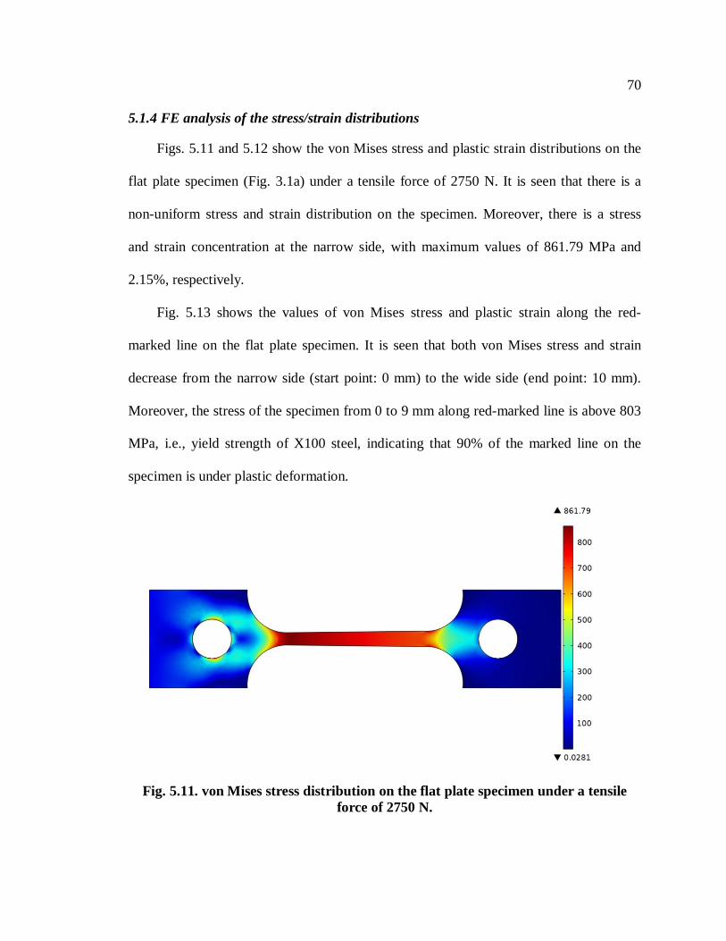
70

5.1.4 FE analysis of the stress/strain distributions

Figs. 5.11 and 5.12 show the von Mises stress and plastic strain distributions on the

flat plate specimen (Fig. 3.1a) under a tensile force of 2750 N. It is seen that there is a

non-uniform stress and strain distribution on the specimen. Moreover, there is a stress

and strain concentration at the narrow side, with maximum values of 861.79 MPa and

2.15%, respectively.

Fig. 5.13 shows the values of von Mises stress and plastic strain along the red-

marked line on the flat plate specimen. It is seen that both von Mises stress and strain

decrease from the narrow side (start point: 0 mm) to the wide side (end point: 10 mm).

Moreover, the stress of the specimen from 0 to 9 mm along red-marked line is above 803

MPa, i.e., yield strength of X100 steel, indicating that 90% of the marked line on the

specimen is under plastic deformation.

Fig. 5.11. von Mises stress distribution on the flat plate specimen under a tensile force of 2750 N.

71

Fig. 5.12. Plastic strain distribution of the flat plate specimen under a tensile force of 2750 N.

0 1 2 3 4 5 6 7 8 9 10 11780

790

800

810

820

830

840

850

860

870 von Mises stress Plastic strain

Distance (mm)

Von

Mise

s st

ress

(MPa

)

0.000

0.004

0.008

0.012

0.016

0.020

0.024

Plastic strain

Fig. 5.13. von Mises stress and plastic strain distributions along the red line marked on the flat plate specimen under a tensile force of 2750 N.

72

5.2 Discussion

The pre-strains applied on the steel specimen in this work are larger than the

yielding strain of 0.388%, but smaller than the strain at UTS, i.e., 4.002%, as shown in

Table 5.1. Thus, the applied pre-strain causes plastic deformation of the steel, and,

consequently, the strain-hardening phenomenon. The strain-hardening mechanism is

well-illustrated on the basis of dislocation-dislocation interactions. The plastic

deformation not only increases the mobility of existing dislocations, but also generates

new dislocations [113-115]. For example, a linear dependence of the density of mobile

dislocations on the value of plastic strain has been found on steels [113].

Thus, the pre-strain applied on X100 steel specimen enhances the yielding and

ultimate tensile strengths of the steel (Figs. 5.1 and 5.2) primarily by increasing the

dislocation density and the dislocation-dislocation interaction as well as the resistance to

dislocation motion. The decrease of ductility of the steel with pre-strain, as indicated by

the fracture strain and the percentage of reduction-in-area in Table 5.1 and Fig. 5.2, is due

to the increasing resistance to twinning and slipping of dislocations [116].

Furthermore, the strain-hardening is rarely observed on the pre-strained steel, as

shown in Fig. 5.1. This phenomenon is associated with the intrinsic mechanical

properties of high-strength pipeline steels, such as X100 steel. There is a quite high yield-

to-tensile strength ratio (Y/T) of approximately 0.933 for the steel. Thus, the capacity of a

further hardening is very limited compared to low grades of steel.

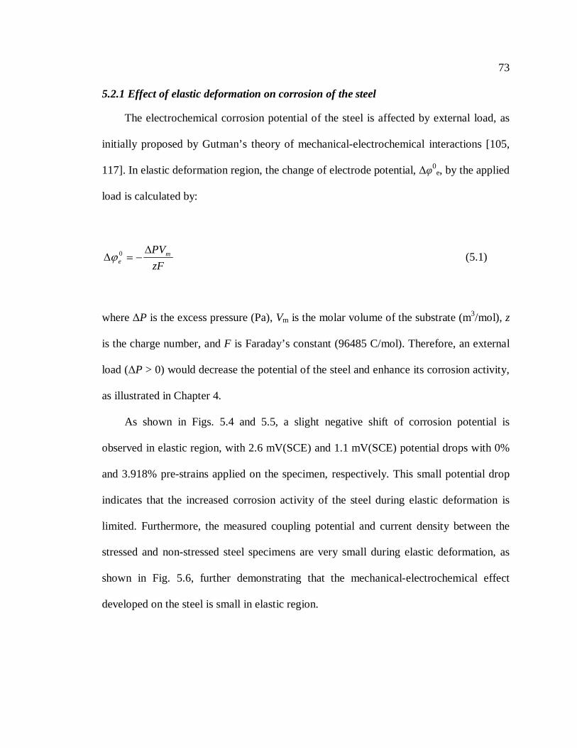
73

5.2.1 Effect of elastic deformation on corrosion of the steel

The electrochemical corrosion potential of the steel is affected by external load, as

initially proposed by Gutman’s theory of mechanical-electrochemical interactions [105,

117]. In elastic deformation region, the change of electrode potential, Δφ0e, by the applied

load is calculated by:

zFPVm

e∆

−=∆ 0ϕ (5.1)

where ΔP is the excess pressure (Pa), Vm is the molar volume of the substrate (m3/mol), z

is the charge number, and F is Faraday’s constant (96485 C/mol). Therefore, an external

load (ΔP > 0) would decrease the potential of the steel and enhance its corrosion activity,

as illustrated in Chapter 4.

As shown in Figs. 5.4 and 5.5, a slight negative shift of corrosion potential is

observed in elastic region, with 2.6 mV(SCE) and 1.1 mV(SCE) potential drops with 0%

and 3.918% pre-strains applied on the specimen, respectively. This small potential drop

indicates that the increased corrosion activity of the steel during elastic deformation is

limited. Furthermore, the measured coupling potential and current density between the

stressed and non-stressed steel specimens are very small during elastic deformation, as

shown in Fig. 5.6, further demonstrating that the mechanical-electrochemical effect

developed on the steel is small in elastic region.

74

5.2.2 Effect of plastic deformation on corrosion of the steel

During plastic deformation, particularly, in the stage of strain hardening, the density

of mobile dislocations is increased with the increasing stress by activation of new

dislocations. The density of new dislocations, ΔN, is calculated by [105, 117]:

−

∆=∆ 1exp

max0 TkN

nNNα

τ (5.2)

where N0 is the initial density of dislocations prior to plastic deformation, Δτ is the

hardening intensity, n is the number of dislocations in a dislocation pile-up, α is a

coefficient of 109 - 1011 cm-2, k is Boltzmann constant, Nmax is the maximum dislocation

density, and T is temperature. The plastic strain at the hardening stage can be expressed

by:

−

∆= 1exp

max

0

TkNnN

p ατ

ανε (5.3)

where υ is the orientation-dependent factor, equalling to 0.4 - 0.5 for tensile deformation.

According to Gutman’s mechanical-electrochemical interactions theory, the change

of electrode potential, 0pϕ∆ , of metals in plastic deformation can be expressed by:

zFkNRn

pmax

0

ατϕ ∆

−=∆ (5.4)

75

where R is the gas constant 8.314 (J/K mol). Substitute Eq. 5.3 into Eq. 5.4 to eliminate

parameters n , Δτ, k and Nmax, and the shift of electrochemical equilibrium potential as a

function of plastic strain, εp, is established:

+−=∆ 1ln

0

0pp NzF

TR ευαϕ (5.5)

To calculate of the theoretical potential shift by Eq. 5.5, it is assumed that T = 295 K,

R = 8.314 J/K mol, z = 2, F = 96485 C/mol, υ = 0.45, and α = 1.67×1011 /cm2. N0 is

assumed roughly for steel under various pre-plastic strains to be 108 /cm2, 2×108 /cm2,

5×108 /cm2 and 109 /cm2. εp varies from 0 to 3.530% to be in a consistent range with the

experimental plastic strains, i.e., 0%, 0.597%, 2.238% and 3.530%. The theoretical

calculation of electrochemical equilibrium potential shift is shown in Fig. 5.14. It is

apparent that the potential shifts negatively with plastic strain, indicating an enhanced

electrochemical corrosion activity of the steel. The calculated result is well consistent

with the measurements in this work in Fig. 5.3. Moreover, the enhanced corrosion

activity of steel by pre-strain is clearly indicated by the decreasing size of semicircle, i.e.,

charge-transfer resistance for corrosion reaction, in EIS plots in Fig. 5.7.

76

0.000 0.005 0.010 0.015 0.020 0.025 0.030 0.035 0.040-0.050

-0.045

-0.040

-0.035

-0.030

-0.025

-0.020

-0.015

-0.010

-0.005

0.000

0.005

Pote

ntia

l shi

ft (V

,SCE

)

Plastic strain

Theoretical N0=1x108 cm-2

Theoretical N0=2x108 cm-2

Theoretical N0=5x108 cm-2

Theoretical N0=1x109 cm-2

Fig.5.14. Theoretical calculation of the electrochemical equilibrium potential shift as a function of plastic strain of the steel specimen with various initial dislocation

densities.

5.2.3 Corrosion of steel during tensile testing

The M-E effect on the steel specimen experiencing both elastic and plastic

deformation stages during tensile testing should be based on Eqs. 5.1 and 5.5 to consider

simultaneously the shift of corrosion potential, 0Tϕ∆ :

+−

∆−=∆ 1ln

0

0p

mmT NzF

TRzF

VP ευαϕ (5.6)

where ΔPm is the excess pressure to elastic deformation limit. In this work, a uniaxial

stress is applied on the specimen, and ΔPm equals to 1/3 of the yield strength of the steel

77

[105]. Furthermore, the net anodic dissolution current density, i, of a plastically stressed

steel electrode is given by [105]:

cmm

a iTkN

nRT

VPii −

∆+

∆=

max

expα

τ

= cmm

pa iRT

VPN

i −

∆

+ exp1

0

ευα (5.7)

where ia and ic are the anodic and cathodic current density, respectively. Assume that the

external stress on the specimen does not affect the ion activity in the solution, ic remains

constant. It is thus apparent that the anodic dissolution rate of the steel is accelerated by

external stress/strain. The current density measured in Fig. 5.6 flows between the stressed

and non-stressed specimens (the former acts as anode and the latter as cathode), and the

variation of anodic current density is very small in elastic deformation. It is thus seen that

the M-E effect in elastic stage is unapparent. However, it becomes significant in plastic

stage, as indicated by a rapid increase of anodic current density in Fig. 5.6.

Furthermore, analysis of the M-E effect on corrosion of the stressed steel has to

consider both anodic and cathodic reactions simultaneously. As discussed, the anodic

dissolution reaction would be accelerated by applied stress/strain which increases the

electrochemical activity of the steel. The cathodic reaction, i.e., the hydrogen evolution

due to reduction of water in deoxygenated, neutral pH solution, would also be affected by

external stress. This is demonstrated by the increasing cathodic current density measured

at -1 V(SCE) with pre-strain applied on the steel in Fig. 5.8. It is primarily attributed to

78

the redistribution of electrochemical heterogeneity and increasing area of the cathodic

process. The increase of slip steps, microcracks and surface defects generated during

plastic deformation would reduce the activation energy of hydrogen evolution [117].

5.2.4 Corrosion of pipelines with a non-uniform plastic stress/strain distribution

This work demonstrates both theoretically and experimentally that the plastic

stress/strain would enhance the corrosion activity of steel. When a steel specimen

contains a non-uniform plastic stress/strain distribution, it is expected that the local

corrosion rate of the steel would be different, subjective to various stress/strain conditions.

The micro-electrochemical techniques provide promising methods to measure locally the

corrosion activity and map the distributions of electrochemical impedance or dissolution

current density with different stress/strain zones. Figs. 5.9 and 5.10 show clearly that, as

the microprobe scans from the narrow side to the wide side on the flat plate specimen,

there are increasing impedance and decreasing current density recorded. Both stress and

strain simulations (Figs. 5.11 and 5.12) indicate that there exists stress/strain

concentration at the narrow side. Moreover, over 90% of the scanning zone is in plastic

deformation under the loading condition in this work, as indicated in Fig. 5.13.

Apparently, the quite different corrosion activity recorded on the specimen is due to the

non-uniform distribution of plastic stress and strain. This result is different from previous

work in Chapter 4, where a non-uniform elastic stress/strain distribution would not be

able to generate a detectable difference of corrosion activity. In reality, a non-uniform

stress/strain distribution on pipelines that is due to a wide variety of reasons, such as

mechanical dent, corrosion, surface defects, etc., would cause preferential corrosion

79

occurring locally, resulting in localized corrosion and the initiation of corrosion pits and

even cracks.

5.3 Summary

The X100 steel shows an apparent strain hardening phenomenon upon application of

pre-strain. Both yield and ultimate tensile strengths are increased, while the ductility is

reduced with the increasing amount of pre-strain.

While the steel corrosion is enhanced by applied strain, the increasing corrosion

activity of the steel during elastic deformation is limited. Thus, the mechano-

electrochemical effect developed on the steel is small in elastic region. Plastic strain

would increase the mechano-electrochemical effect on pipeline corrosion significantly, as

demonstrated by the measured corrosion potential, coupling current density and EIS

measurements.

While both anodic and cathodic reactions are enhanced by the applied strain. The

negative shift of corrosion potential indicates that the effect on anodic reaction is more

significant.

In reality, a non-uniform distribution of plastic stress and strain on pipelines would

cause quite different corrosion activities of the steel. This would cause preferential

corrosion occurring locally, resulting in localized corrosion and the initiation of corrosion

pits and even cracks.

80

Chapter Six: Development of a finite element model for simulation and prediction of the M-E effect at corrosion defects

In this Chapter, a FE model is developed upon previous work in Chapter 5 to study

both experimentally and numerically the mechanical-electrochemical interaction, i.e., the

mechano-electrochemical (M-E) effect on pipeline corrosion at defect on X100 steel

pipeline under synergistic effects of soil strain and internal pressure in a near-neutral pH

solution. The initial parametrical conditions for FE modelling are derived from

experimental tests. The reliability of the model is validated by various mechanical and

corrosion measurements. The parameters simulated include the stress distribution,

corrosion potential, and anodic and cathodic current densities as a function of the defect

size and the longitudinal tensile strain induced by soil movement. A sufficiently reliable

method is developed to enable simulation and prediction of localized corrosion on

pipelines under complex stress and strain conditions.

6.1 Numerical simulation and analysis

6.1.1 Initial and boundary geometrical parameters

The FE simulation of the M-E effect of pipeline corrosion is performed using a

commercial COMSOL Multiphysics 4.2a software. The geometrical model of the steel

pipe containing a corrosion defect is shown in Fig. 6.1a, where the pipe wall thickness is

19.1 mm (3/4 in.) and the outer diameter of the pipe is 812.8 mm (32 in.). The length of

the pipe segment for FE simulation is 2 m. The corrosion defect is elliptically shaped,

with a length of 200 mm, and depths of 20%, 40%, 60% and 80% of the pipe wall

81

thickness, i.e., 3.82 mm, 7.64 mm, 11.46 mm and 15.28 mm, respectively. In reality, the

aspect ratio of defect may change during corrosion. This work assumes an unchanged

length with a growing depth for corrosion defect in order to investigate propagation of the

corrosion defect along the pipe wall direction.

Fig. 6.1. The geometrical model of the steel pipe containing a corrosion defect for FE simulation (a) 3D model, (b) 2D model.

The boundary condition for FE simulation includes that the solution boundary is

electrically isolated, except the solution/steel interface which is set as a free boundary.

While the left end of the steel pipe is fixed, the right end is loaded with prescribed tensile

strains as described below. The bottom of the pipe is set as electric grounding. The mesh

type used is triangular.

(b)

(a)

82

The 3D geometry of pipe segment is simplified into a 2D model due to the

symmetrical property, as shown in Fig. 6.1b. The FE simulation contains three aspects,

i.e., (i) the mechanical elasto-plastic solid stress analysis of the steel pipe, (ii) the

electrochemical potential and current density analyses in solution and at the steel/solution

interface, and (iii) the simulation and analysis of the M-E effect of pipeline corrosion, i.e.,

the interaction of mechanical stress/strain and corrosion of the steel in the solution.

6.1.1. FE simulation of mechanical stress developed on pipelines

An elasto-plastic solid stress simulation is performed on pipe steel. The isotropic

hardening model is selected, and the hardening function, σyhard, is defined as [118]:

yse

pyseffyhard Eσσεσσεσσ −+=−= )()( expexp (6.1)

where σexp is the experimental stress function derived from the measured engineering

stress-strain curve of X100 steel (as shown in Fig. 4.1 in Chapter 4), εeff is total effective

strain, σys is yield strength of the steel, i.e., 803 MPa, εp is plastic strain, σe is effective

stress, E is Young’s modulus of 207,000 MPa, and σe/E is elastic strain. The von Mises

yielding criterion is used for the elasto-plastic simulation. A variety of tensile strains, i.e.,

0%, 0.1%, 0.2%, 0.3% and 0.4%, are applied on the steel pipe along the longitudinal

direction to simulate the soil strain. It is realized that the tensile strain applied is total

strain, and is equal to the total deformation divided by the pipe segment length. Local

strain could be varied due to the presence of corrosion defects.

83

6.1.2. FE simulation of electrochemical corrosion parameters

The electrochemical anodic and cathodic reactions of X100 steel in the

deoxygenated, near-neutral pH NS4 solution (pH=6.8) are the dissolution of Fe and the

hydrogen evolution, respectively [54, 92, 94, 103, 104]:

Anodic reaction: Fe → Fe2+ + 2e (6.2)

Cathodic reaction: 2H2O + 2e → H2+ 2OH- (6.3)

Corrosion of the steel in NS4 solution is activation-controlled [92-95]. The electrode

kinetics for anodic and cathodic reactions is described by:

= a

a

baa ii

η

10,0 (6.4)

= c

c

bcc ii

η

10,0 (6.5)

eqϕϕη −= (6.6)

where subscripts a and c refer to anodic and cathodic reactions, respectively, i is charge-

transfer current density of electrochemical reactions, i0 is exchange current density, φ is

electrode potential, φeq is equilibrium electrode potential, η is activation overpotential,

and b is Tafel slope. The equilibrium potentials of the oxidation of Fe and the hydrogen

evolution are determined by Nernst equations [119]:

84

]log[2

0592.0 20,,

++= Feeqaeqa ϕϕ (6.7)

0592.0]log[0592.00,, −=+= +Heqceqc ϕϕ pH (6.8)

The standard equilibrium potentials for reaction (6.2) and (6.3) are -0.409 V(standard

hydrogen electrode, SHE) and 0 V(SHE), respectively [119]. Assume the concentration

of ferrous ions in NS4 solution is 10-6 M. With a solution pH of 6.8, the equilibrium

potentials of reactions (6.2) and (6.3) are calculated as -0.859 V(SCE) and -0.644

V(SCE), respectively. The exchange current densities of the anodic and cathodic

reactions are derived from the measured polarization curve, as shown in Fig. 6.2, through

the Tafel extrapolation method. The electrochemical corrosion parameters used as the

initial inputs for FE simulation are summarized in Table 6.1.

Table 6.1: The initial electrochemical parameters for FE simulation derived from Fig. 6.2.

Electrochemical Reactions

log i0 (A/cm2)

Equilibrium Potential φeq,0 (V, SCE)

Tafel slope (V/decade) i0 (A/cm2)

Cathodic H evolution -5.837 -0.644 -0.207 1.457×10-6

Corrosion (iH = iFe) -5.457 -0.722 N/A 3.489×10-6

Anodic Fe oxidation -6.628 -0.859 0.118 2.353×10-7

85

-8.0 -7.5 -7.0 -6.5 -6.0 -5.5 -5.0 -4.5 -4.0-1.0

-0.9

-0.8

-0.7

-0.6

-0.5

icorri0,H

Pote

ntia

l (V,

SCE)

log i (A/cm2)

i0,Fe

Fig. 6.2. Potentiodynamic polarization curve measured on X100 steel in NS4 solution.

6.1.2 Multi-physical fields coupling FE simulation of M-E effect of pipeline corrosion

(I) Anodic reaction

Effects of elastic and plastic deformations on equilibrium potential of the anodic

reaction have been derived by Gutman [120] and further developed for pipeline corrosion

in Chapter 5:

Elastic deformation: zFPVme

eqa∆

−=∆ ,ϕ (6.9)

Plastic deformation:

+−=∆ 1ln

0, p

peqa NzF

TR ευαϕ (6.10)

Continuous elasto-plastic tension:

+−

∆−= 1ln

0

0,, p

mmeqaeqa NzF

TRzF

VP ευαϕϕ (6.11)

86

where eeqa,ϕ∆ and p

eqa,ϕ∆ are shifts of equilibrium potential of anodic reaction under

elastic and plastic deformations, respectively, 0,eqaϕ is standard equilibrium potential of

anodic reaction, ΔP is excess pressure (Pa) that is equal to 1/3 of uniaxial tensile stress,

ΔPm is excess pressure to elastic deformation limit that is equal to 1/3 of yield strength of

steel, Vm is molar volume of the steel (7.13×10-6 m3/mol), z is number of charge (z=2 for

steel), R is ideal gas constant (8.314 J/mol K), T is absolute temperature (T=298.15 K), F

is Faraday’s constant (F=96485 C/mol), υ is an orientation-dependent factor (υ=0.45), α

is a coefficient of 1.67×1011 cm-2, N0 is initial density of dislocations prior to plastic

deformation (1×108 cm-2), and εp is plastic strain obtained through mechanical elasto-

plastic simulation [120].

(II) Cathodic reaction

In Chapter 5, it was found experimentally that the cathodic reaction, i.e., hydrogen

evolution in a deoxygenated neutral pH solution, would be enhanced by plastic

deformation. The theory has been illustrated by Gutman through Evans diagram, where a

mechanical deformation can lead to a redistribution of electrochemical heterogeneities

and increasing area for cathodic reaction [120]. Moreover, an increase of slip steps,

micro-cracks and surface defects generated during plastic deformation would reduce the

activation energy of the hydrogen evolution. To simplify the FE modeling, only the

increase in exchange current density upon plastic deformation is considered in this work.

With an extensive FE simulation, modification and verification with experimental data, a

semi-empirical expression is derived to describe the M-E effect on cathodic reaction:

87

)(6,0 10 c

mMises

bFV

cc ii −=σ

(6.12)

where i0,c is exchange current density of hydrogen evolution on X100 steel in the absence

of external stress/strain, σMises is von Mises stress calculated from FE simulation, and bc is

cathodic Tafel slope.

(III) Distributions of potential and current density in solution and steel electrode

According to the electrical field theory [121], the general equations for defining

distribution of the current field in solution and steel electrode during electrochemical

reactions are:

kk Qi =⋅∇ (6.13)

kkki ϕσ ∇−= (6.14)

where Qk denotes a general source term, k is an index where liquid (l) for electrolyte (e.g.,

NS4 solution) or solid (s) for the metal electrode (e.g., X100 steel electrode), σk is

conductivity, and φk is potential. The conductivities of solution and steel electrode are set

as 0.096 S/m and 106 S/m, respectively.

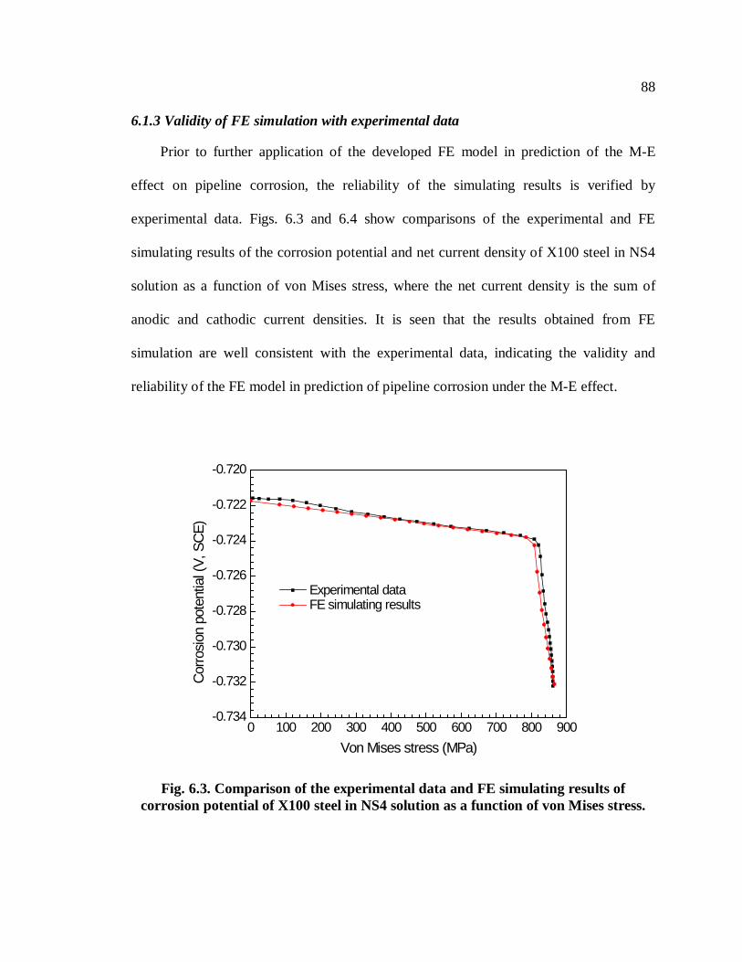
88

6.1.3 Validity of FE simulation with experimental data

Prior to further application of the developed FE model in prediction of the M-E

effect on pipeline corrosion, the reliability of the simulating results is verified by

experimental data. Figs. 6.3 and 6.4 show comparisons of the experimental and FE

simulating results of the corrosion potential and net current density of X100 steel in NS4

solution as a function of von Mises stress, where the net current density is the sum of

anodic and cathodic current densities. It is seen that the results obtained from FE

simulation are well consistent with the experimental data, indicating the validity and

reliability of the FE model in prediction of pipeline corrosion under the M-E effect.

0 100 200 300 400 500 600 700 800 900-0.734

-0.732

-0.730

-0.728

-0.726

-0.724

-0.722

-0.720

Corro

sion

pote

ntia

l (V,

SCE

)

Von Mises stress (MPa)

Experimental data FE simulating results

Fig. 6.3. Comparison of the experimental data and FE simulating results of corrosion potential of X100 steel in NS4 solution as a function of von Mises stress.

89

0 100 200 300 400 500 600 700 800 900-1.0

-0.5

0.0

0.5

1.0

1.5

2.0

2.5

Net c

urre

nt d

ensit

y (µ

A/cm

2 )

Von Mises stress (MPa)

Experimental data FE simulating results

Fig. 6.4. Comparison of experimental data and the FE simulating results of net current density of X100 steel in NS4 solution as a function of von Mises stress.

6.2 Results

6.2.1 FE simulation of the stress concentration at corrosion defect and the potential and net current density distributions in solution

Fig. 6.5 shows the distributions of the potential field in solution and von Mises

stress at corrosion defect (11.46 mm in depth) under various longitudinal tensile strains.

There are two color legends in the figure, where the top right color bar indicates potential

(V, SCE) or net current density (μA/cm2), and the bottom right one is for von Mises

stress (MPa). It is seen that, under 0.1% of tensile strain, the stress level at the corrosion

defect is slightly higher than that of the pipe wall, as indicated by the minor change of

color on the stress bar. Moreover, the potential field in solution is very uniform. At the

tensile strain of 0.2%, local stress increases apparently at the corrosion defect, while

90

potential is still uniform in the solution. When the tensile strain is increased to 0.3% and

0.4%, the local stress further increases, as indicated by the red and dark red color on the

stress bar. A non-uniform distribution of the potential field becomes notable in the

solution, especially at the strain of 0.4%. A semi-circular area with the most negative

potential is observed adjacent to the corrosion defect, where the maximum stress is

generated. Therefore, the larger the tensile strain, the more negative the potential and the

higher the local stress concentration.

Fig. 6.5. Distributions of the potential field in NS4 solution and von Mises stress at the corrosion defect (11.46 mm in depth) under various longitudinal strains.

91

Fig. 6.6. Distributions of the potential field in NS4 solution and von Mises stress at the corrosion defect with various depths under a fixed 0.3% longitudinal tensile

strain.

Fig. 6.6 shows distributions of the potential field in solution and von Mises stress at

corrosion defect with various depths under a fixed 0.3% longitudinal tensile strain. It is

seen that the presence of relatively shallow corrosion defects, i.e., 3.82 mm and 7.64 mm

in depth, does not affect the potential field in solution. A stress concentration is detected

at the defect by a slight change of color on the stress bar. With the corrosion depth

increasing to 11.46 mm and 15.28 mm, the stress concentration at the defect center

further increases, while that at edges of the defect decreases. The potential in solution is

negatively shifted, and an uneven potential distribution is observed, where the potential in

the region adjacent to the defect center is much more negative than that of other area. The

92

deeper the corrosion defect, the more negative the potential and the higher the stress

concentration is generated.

Fig. 6.7 shows distributions of net current density in solution and von Mises stress at

corrosion defect (11.46 mm in depth) under various longitudinal tensile strains. It is seen

that the application of 0.1% and 0.2% tensile strains does not affect the net current

density at a visible level, and the local stress concentration increases slightly. With the

strain increasing to 0.3% and 0.4%, the stress at the corrosion defect is enhanced

obviously. Moreover, the net current flow in solution is observed, as indicated by vectors

pointing from the defect center to the sides. The larger the tensile strain, the higher the

net current density and the stress concentration.

Fig. 6.7. Distributions of net current density in NS4 solution and von Mises stress at corrosion defect (11.46 mm in depth) on the pipe wall under various longitudinal

tensile strains.

93

Fig. 6.8 shows distributions of net current density in solution and von Mises stress at

corrosion defect with various depths under a fixed 0.3% longitudinal tensile strain. It is

seen that the presence of shallow corrosion defects, e.g., 3.82 mm and 7.64 mm in depth,

does not affect the net current density distribution in solution, but increases the stress

concentration at the defect. With the corrosion depth increasing to 11.46 mm and 15.28

mm, the stress concentration is further enhanced. Moreover, the net current flow in

solution becomes apparent, as indicated by vectors pointing from the defect center to the

sides. The deeper the corrosion defect, the higher the net current density and the stress

concentration.

Fig. 6.8. Distributions of net current density in solution and von Mises stress at corrosion defect with various depths under a fixed 0.3% longitudinal strain.

94

6.2.2 FE simulation of linear distributions of stress at the bottom of corrosion defect

Fig. 6.9 shows the linear distribution of von Mises stress along the bottom of a 11.46

mm deep corrosion defect on the pipe steel under various longitudinal tensile strains from

0% to 0.4%. It is seen that the stress is distributed symmetrically to the center of the

defect, and the highest stress occurs at the defect center. With the increase of tensile

strain, the stress level is enhanced. Moreover, the strains of 0.3% and 0.4% result in a

local stress exceeding yield strength (~803 MPa) of X100 steel. Thus, plastic deformation

occurs at the central area of the defect, while other area is in elastic range.

0 20 40 60 80 100 120 140 160 180 200

0

100

200

300

400

500

600

700

800

900

Von

Mise

s st

ress

(MPa

)

Defect length (mm)

0% 0.1% 0.2% 0.3% 0.4%

Fig. 6.9. Linear distribution of von Mises stress along the bottom of the 11.46 mm deep corrosion defect on the pipe under various longitudinal tensile strains.

Fig. 6.10 shows the linear distribution of von Mises stress along the bottom of

corrosion defect with various depths under a 0.3% longitudinal tensile strain. Similar to

95

Fig. 6.9, the stress is distributed symmetrically, with the highest stress at the defect center.

However, unlike the stress distribution in Fig. 6.9, the stress is more concentrated at the

center with the increase of the defect depth. The stress at the defect center increases while

that at both sides decreases when corrosion defect increases in depth.

0 20 40 60 80 100 120 140 160 180 200

0

100

200

300

400

500

600

700

800

900

Von

Mise

s st

ress

(MPa

)

Defect length (mm)

3.82 mm 7.64 mm 11.46 mm 15.28 mm

Fig. 6.10. Linear distribution of von Mises stress along the bottom of corrosion defect with various depths under 0.3% longitudinal tensile strain.

6.2.3 FE simulation of linear distributions of corrosion potential and anodic/cathodic current densities at corrosion defect

Fig. 6.11 shows the linear distribution of corrosion potential along the bottom of

corrosion defect with 11.46 mm in depth on the pipe under various longitudinal tensile

strains in NS4 solution. It is seen that, in the absence of tensile strain, corrosion potential

remains constant of -0.722 V(SCE) along the defect bottom. Upon application of strain,

96

corrosion potential is shifted negatively. At strains of 0.1% and 0.2%, the corrosion

potential is distributed uniformly, with a slightly more negative potential at the defect

center. When the applied strain increases to 0.3% and 0.4%, the corrosion potential at the

defect center is much more negative that that at both sides of the defect.

0 20 40 60 80 100 120 140 160 180 200-0.734

-0.732

-0.730

-0.728

-0.726

-0.724

-0.722

-0.720

Corro

sion

pote

ntia

l (V,

SCE

)

Defect length (mm)

0% 0.1% 0.2% 0.3% 0.4%

Fig. 6.11. Linear distribution of corrosion potential along the bottom of corrosion defect with 11.46 mm in depth on the pipe under various longitudinal tensile strains

in NS4 solution.

Fig. 6.12 shows the linear distribution of corrosion potential along the bottom of

corrosion defect with various depths in NS4 solution where a 0.3% longitudinal tensile

strain is applied. It is seen that, at corrosion depths of 3.82 mm and 7.64 mm, there is an

even distribution of corrosion potential, i.e., the presence of corrosion defect does not

affect the corrosion potential across the defect. With the depth increasing to 11.46 mm

97

and 15.28 mm, the corrosion potential is shifted negatively, with the most negative

potential at the defect center.

0 20 40 60 80 100 120 140 160 180 200-0.734

-0.732

-0.730

-0.728

-0.726

-0.724

-0.722Co

rrosio

n po

tent

ial (

V, S

CE)

Defect length (mm)

3.82 mm 7.64 mm 11.46 mm 15.28 mm

Fig. 6.12. Linear distribution of corrosion potential along the bottom of corrosion defect with various depths in NS4 solution where a 0.3% longitudinal tensile strain

is applied.

Fig. 6.13 shows the linear distribution of anodic current density along the bottom of

the 11.46 mm corrosion defect under various longitudinal tensile strains in NS4 solution.

It is seen that, in the absence of tensile strain, the anodic current density is constant at 3.5

μA/cm2 along the defect bottom. With the strain increasing to 0.1% and 0.2%, the anodic

current density increases, but the distribution of the current density is nearly uniform

across the defect. When the strain further increases to 0.3% and 0.4%, the current density

at the center of the defect increases significantly to 5.4 μA/cm2 and 6.3 μA/cm2,

respectively, while that decreases slightly at the defect sides.

98

0 20 40 60 80 100 120 140 160 180 2003.0

3.5

4.0

4.5

5.0

5.5

6.0

6.5

Anod

ic cu

rrent

den

sity

(µA/

cm2 )

Defect length (mm)

0% 0.1% 0.2% 0.3% 0.4%

Fig. 6.13. Linear distribution of anodic current density along the bottom of the 11.46 mm corrosion defect under various longitudinal tensile strains in NS4 solution.

0 20 40 60 80 100 120 140 160 180 2003.0

3.5

4.0

4.5

5.0

5.5

6.0

6.5

7.0

Anod

ic cu

rrent

den

sity

(µA/

cm2 )

Defect length (mm)

3.82 mm 7.64 mm 11.46 mm 15.28 mm

Fig. 6.14. Linear distribution of anodic current density along the bottom of corrosion defect with various depths in NS4 solution, where a 0.3% longitudinal

tensile strain is applied.

99

Fig. 6.14 shows the linear distribution of anodic current density along the bottom of

corrosion defect with various depths in NS4 solution, where a 0.3% longitudinal tensile

strain is applied. It is seen that there is little difference of anodic current densities

obtained at corrosion depths of 3.82 mm and 7.64 mm. When the corrosion depth

increases to 11.46 mm and 15.28 mm, the anodic current density at the defect center

increases to 5.5 μA/cm2 and 6.7 μA/cm2, respectively.

Fig. 6.15 shows the linear distribution of cathodic current density (hydrogen

evolution) along the bottom of a 11.46 mm corrosion defect under various longitudinal

tensile strains in NS4 solutions. It is seen that, in the absence of tensile strain, the

cathodic current density along the defect bottom is constant at -3.5 μA/cm2. With the

increase of tensile strain, the cathodic current density increases negatively. Moreover,

there is the most negative current density at the defect center.

Fig. 6.16 shows the linear distribution of cathodic current density along the bottom

of corrosion defect with various depths under a 0.3% longitudinal tensile strain in NS4

solution. It is seen that the increase of the defect depth results in a negative increase of

cathodic current density at the defect center. However, at both sides of the corrosion

defect, the current density becomes less negative.

100

0 20 40 60 80 100 120 140 160 180 200-4.5-4.4

-4.3-4.2

-4.1-4.0

-3.9-3.8

-3.7-3.6

-3.5-3.4

Cath

odic

curre

nt d

ensit

y (µ

A/cm

2 )

Defect length (mm)

0% 0.1% 0.2% 0.3% 0.4%

Fig. 6.15. Linear distribution of cathodic current density along the bottom of the 11.46 mm corrosion defect under various longitudinal tensile strains in NS4

solutions.

0 20 40 60 80 100 120 140 160 180 200-4.5

-4.4

-4.3

-4.2

-4.1

-4.0

-3.9

-3.8

-3.7

-3.6

-3.5

Cath

odic

curre

nt d

ensit

y (µ

A/cm

2 )

Defect length (mm)

3.82 mm 7.64 mm 11.46 mm 15.28 mm

Fig. 6.16. Linear distribution of cathodic current density along the bottom of corrosion defect with various depths under 0.3% longitudinal tensile strain.

101

Fig. 6.17 shows the linear distribution of net current density along the bottom of

corrosion defect (11.46 mm in depth) under various longitudinal tensile strains in NS4

solution. It is seen that the net current densities are nearly zero under tensile strains of 0%,

0.1% and 0.2%. With the tensile strain increasing to 0.3% and 0.4%, the net current

density at the defect center increases positively, while that at the defect sides were in

negative range.

0 20 40 60 80 100 120 140 160 180 200-1.0

-0.5

0.0

0.5

1.0

1.5

2.0

Net c

urre

nt d

ensit

y (µ

A/cm

2 )

Defect length (mm)

0% 0.1% 0.2% 0.3% 0.4%

Fig. 6.17. Linear distribution of net current density along the bottom of corrosion defect (11.46 mm in depth) under various longitudinal tensile strains in NS4 solution.

Fig. 6.18 shows the linear distribution of net current density along the bottom of

corrosion defect with various depths and under a 0.3% longitudinal tensile strain in NS4

solution. It is seen that the net current density is almost zero at corrosion defects of 3.82

mm and 7.64 mm in depth. With the defect depth increasing to 11.46 mm and 15.28 mm,

102

the net current density at the defect center increases positively, while it becomes more

negative at both sides.

0 20 40 60 80 100 120 140 160 180 200-1.0

-0.5

0.0

0.5

1.0

1.5

2.0

2.5

Net c

urre

nt d

ensit

y (µ

A/cm

2 )

Defect length (mm)

3.82 mm 7.64 mm 11.64 mm 15.28 mm

Fig. 6.18. Linear distribution of net current density along the bottom of corrosion defect with various depths and under 0.3% longitudinal tensile strain in NS4

solution.

Fig. 6.19 shows the anodic and cathodic current densities at the bottom of corrosion

defect as a function of von Mises stress. It is seen that, in the elastic deformation region,

with the increase of von Mises stress, the absolute values of both anodic and cathodic

current densities increase slightly. When the stress exceeds the yield strength of the steel,

i.e., plastic deformation starts, both anodic and cathodic current densities are increased

significantly. The knee points of both curves are consistent with the yielding point of

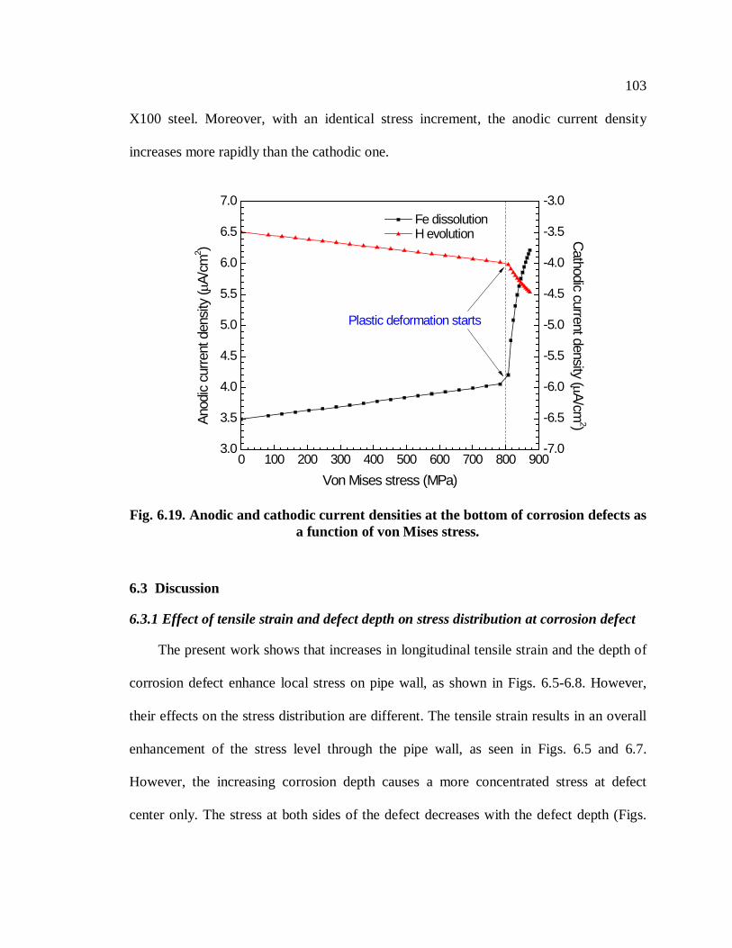
103

X100 steel. Moreover, with an identical stress increment, the anodic current density

increases more rapidly than the cathodic one.

0 100 200 300 400 500 600 700 800 9003.0

3.5

4.0

4.5

5.0

5.5

6.0

6.5

7.0 Fe dissolution H evolution

Von Mises stress (MPa)

Anod

ic cu

rrent

den

sity

(µA/

cm2 )

Plastic deformation starts

-7.0

-6.5

-6.0

-5.5

-5.0

-4.5

-4.0

-3.5

-3.0

Cathodic current density (µA/cm2)

Fig. 6.19. Anodic and cathodic current densities at the bottom of corrosion defects as a function of von Mises stress.

6.3 Discussion

6.3.1 Effect of tensile strain and defect depth on stress distribution at corrosion defect

The present work shows that increases in longitudinal tensile strain and the depth of

corrosion defect enhance local stress on pipe wall, as shown in Figs. 6.5-6.8. However,

their effects on the stress distribution are different. The tensile strain results in an overall

enhancement of the stress level through the pipe wall, as seen in Figs. 6.5 and 6.7.

However, the increasing corrosion depth causes a more concentrated stress at defect

center only. The stress at both sides of the defect decreases with the defect depth (Figs.

104

6.6 and 6.8). This is an interesting and very important phenomenon that is present and

verified at the first time in this area.

When a tensile strain is applied on pipelines containing corrosion defect, the

resulting force (F) in individual cross section of the pipe along the longitudinal direction

is identical according to the principle of mechanics balance. Since stress is inversely

proportional to area, there is a lower stress at two sides of the defect where there is a

larger cross-sectional area, and a higher stress at the defect center with a smaller area.

Moreover, the stress level at different locations changes synchronously with tensile strain,

as seen in Fig. 6.9. However, an increase in depth of corrosion defect makes its central

bottom narrower and its sides relatively opener. Consequently, a high stress concentration

is generated at the central bottom when the pipe is under a certain tensile strain (Fig.

6.10). This non-uniform stress distribution across the corrosion defect is attributed

primarily to the geometry of the corrosion defect.

6.3.2 M-E effect on corrosion potential of steel and the potential field distribution in solution

As stated, the anodic and cathodic reactions of X100 steel in NS4 solution are the Fe

dissolution and hydrogen evolution, respectively, as shown in Reactions (5.2) and (5.3).

Previous work in Chapter 5 demonstrated that the anodic and cathodic reactions would be

affected by mechanical stress/strain, resulting in a negative shift of equilibrium potential

of the steel and an accelerated hydrogen evolution.

In the present work, the M-E effect of pipeline corrosion in the trapped electrolyte

under disbonded coating is simulated by the FE model to integrate the multi-physical

105

fields coupling processes, including mechanical field in the steel, electrochemical field at

the steel/solution interface and electric fields in solution and steel. Therefore, it is

expected that the simulated process and the derived results are more representative of the

reality of pipelines in the field. In particular, the M-E effect on the enhancement of

anodic activity of the steel is described in Eqs. 6.9–6.11 as shown by a negative shift of

equilibrium potential of steel. The effect on accelerated hydrogen evolution is represented

by an empirical equation in Eq. 6.12 through an increase of cathodic exchange current

density. It is realized that some other factors may affect the anodic and cathodic reactions.

For simplicity, these factors are either neglected or combined with the effects in Eqs. 6.9–

6.12 for FE modeling. Reliability of the simulated results is verified with experimental

data, and the results show a very good consistency in Figs. 6.3 and 6.4.

The present work shows that the corrosion potential distribution along the bottom of

corrosion defect does not have an apparent change when tensile strains of 0.1% and 0.2%

are applied, as shown in Fig. 6.11, which is due to the fact that the corrosion defect area

is under elastic deformation under the given conditions. Similarly, the application of

0.3% tensile strain on pipe that contain 3.82 mm and 7.64 mm corrosion defects

introduces an elastic deformation at the defect, and thus, no apparent change of corrosion

potential is observed in Fig. 6.12. The resulting local stress at corrosion defect with

various depths under various tensile strains can be found in Figs. 6.5-6.8. When the

tensile strain or the corrosion depth is further increased, plastic deformation occurs at the

bottom of the defect. This results in a notable shift of corrosion potential negatively along

the defect bottom.

106

Furthermore, there is an uneven potential field distribution in the solution, as shown

in Figs. 6.5 and 6.6. When the pipe is under an elastic deformation, e.g., under tensile

strains of 0.1% and 0.2% or with corrosion depths of 3.82 mm and 7.64 mm, the potential

at corrosion defect is identical to that of other regions in the solution. When the tensile

strain or the corrosion depth is increased to induce a local plastic deformation at the

defect, the potential field in solution is non-uniform, with the most negative potential

generated adjacent to the center of the corrosion defect. The potential gradient existing at

different locations provides a driving force of current flow in solution.

6.3.3 M-E effect on anodic/cathodic current density and the current field distribution in solution

Since stressing affects the potential distribution of steel, as demonstrated, it is

assumed that the corrosion at defect is composed of a series of local galvanic cells, where

the region with a high stress, such as the defect center, serves as an anode, and that under

a low stress, such as the sides of the defect, as the cathode. Electrons generated at the

anode flow through the pipe wall into the cathode, and ferrous ions flow towards the

cathode through solution. As a consequence, anodic dissolution at the defect center is

further accelerated, while it is mitigated slightly at the sides of the defect, as shown in

Figs. 6.13 and 6.14. For example, for the 11.46 mm deep corrosion defect in Fig. 6.13, in

the absence of tensile strain, the steel dissolution is uniform inside the defect with a

dissolution current density of 3.49 μA/cm2. However, when a 0.4% tensile strain is

applied, the current density at the defect center is up to 6.22 μA/cm2, while that at both

sides are 3.24 μA/cm2 only. This locally accelerated corrosion at the defect center is

107

further enhanced by the increasing depth of the defect, i.e., the deeper the corrosion

defect, the higher the dissolution current density at the defect center is, as shown in Fig.

6.14.

Hydrogen evolution is also accelerated by mechanical factors. The presence of local

galvanic cells affects distribution of cathodic current density along the defect bottom, as

shown in Figs. 6.15 and 6.16. In the absence of tensile strain, the cathodic current density

is numerically equal to the anodic current density, i.e., -3.49 μA/cm2, indicating that the

steel is under free corrosion in the defect. In the presence of tensile strain, such as 0.4%

strain, when anodic current density at the defect center increases to 6.22 μA/cm2, the

cathodic current density is up to -4.46 μA/cm2. This unbalanced anodic and cathodic

current densities indicates that the defect center is polarized more anodically due to the

M-E effect, which is terms as "net current density" in this work.

According to the net current density distributions shown in Figs. 6.17 and 6.18, it is

apparent that the central defect experiences an anodic polarization, as indicated by a

positive net current density, and the sides of the defect are under cathodic polarization.

Similarly, the net current density distribution in solution, as shown in Figs. 6.8 and 6.9,

shows that the current flows out of the defect center towards solution, indicating that the

central part is under anodic polarization and corrosion is enhanced. Moreover, the current

flows into the sides of the defect, showing that these areas are under cathodic polarization,

and corrosion would be mitigated.

108

6.3.4 Implications on pipeline corrosion and the risk assessment

During operation in the field, pipelines experience hoop stress and longitudinal soil

strain as well as local stress concentration at corrosion defects. The multi-axial

stress/strain condition should be maintained in the elastic range in order to ensure safety

design. However, the ground movement in the Arctic and sub-Arctic areas is so

significant that the pipeline design follows a strain-based design criterion [1-5], where the

longitudinal tensile strain generated on pipelines is allowed up to 2.5% [27].

This work demonstrates that a stress concentration is generated at corrosion defect,

which can suffer from locally accelerated corrosion at the central bottom, while corrosion

at both sides of the defect is mitigated. This localized corrosion further results in a stress

concentration. Consequently, the local pitting would be developed to potentially cause

pipeline leaking.

Generally, the industry standards and codes, such as CSA-Z662, DNV-OS-F101 and

API-579-FFS [15, 27, 57], have been used to assess pipeline corrosion and predict

remaining service life of pipelines containing corrosion defects. These codes were

developed for evaluation of uniform corrosion rate and/or smooth corrosion defects

present on pipelines that are made of relatively low grades of steel, such as those lower

X80 grade. Defects with a complex geometry and contained on high-strength steel

pipelines have not been considered. It is thus impossible to predict accurately the

corrosion defect propagation and remaining strength of pipelines, especially when they

experience complex, multi-axial stresses and strains. This work provides a promising

approach to industry for reliable defect assessment with considerations of the synergism

of stress concentration and localized corrosion, and more important, a preferential

109

corrosion developing at the central bottom of the corrosion defect to potentially result in

pipeline leaking.

6.4 Summary

A FE model is developed to study the M-E effect of pipeline corrosion through a

multi-physical fields coupling simulation that analyses the solid mechanics field in steel,

electrochemical reactions at the steel/solution interface and the electric field in solution.

The model enables simulation and prediction of the synergism of stress concentration and

localized corrosion on pipelines that experience complex, multi-axial stresses and strains.

An increase of the longitudinal tensile strain and the depth of corrosion defect

enhance local stress on pipe wall. However, their effects on stress distribution are

different. While a tensile strain results in an overall enhancement of stress through the

pipe wall, the increasing corrosion depth causes a more concentrated stress at the defect

center. Stress at both sides of the defect actually decreases with the defect depth.

When corrosion defect is under local an elastic deformation, there is no apparent

mechanical-electrochemical interaction affecting corrosion. When tensile strain or the

corrosion depth is further increased to result in a local plastic deformation, the local

corrosion activity is increased remarkably.

The corrosion at defect is composed of a series of local galvanic cells, where the

region with a high stress, such as the defect center, serves as an anode, and that under low

stress, such as the sides of the defect, as the cathode. Anodic dissolution at the defect

center is further accelerated, while it is mitigated slightly at the sides of the defect. The

110

locally accelerated corrosion at the defect center is further enhanced by the increasing

depth of the corrosion defect.

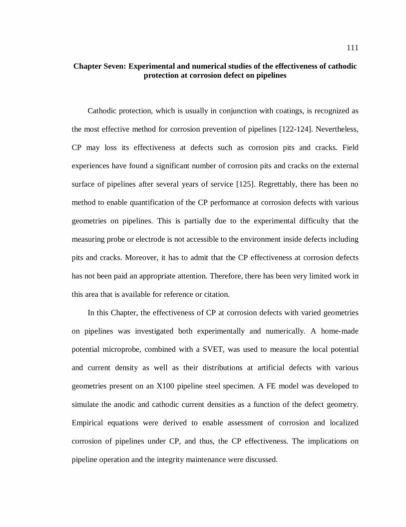
111

Chapter Seven: Experimental and numerical studies of the effectiveness of cathodic protection at corrosion defect on pipelines

Cathodic protection, which is usually in conjunction with coatings, is recognized as

the most effective method for corrosion prevention of pipelines [122-124]. Nevertheless,

CP may loss its effectiveness at defects such as corrosion pits and cracks. Field

experiences have found a significant number of corrosion pits and cracks on the external

surface of pipelines after several years of service [125]. Regrettably, there has been no

method to enable quantification of the CP performance at corrosion defects with various

geometries on pipelines. This is partially due to the experimental difficulty that the

measuring probe or electrode is not accessible to the environment inside defects including

pits and cracks. Moreover, it has to admit that the CP effectiveness at corrosion defects

has not been paid an appropriate attention. Therefore, there has been very limited work in

this area that is available for reference or citation.

In this Chapter, the effectiveness of CP at corrosion defects with varied geometries

on pipelines was investigated both experimentally and numerically. A home-made

potential microprobe, combined with a SVET, was used to measure the local potential

and current density as well as their distributions at artificial defects with various

geometries present on an X100 pipeline steel specimen. A FE model was developed to

simulate the anodic and cathodic current densities as a function of the defect geometry.

Empirical equations were derived to enable assessment of corrosion and localized

corrosion of pipelines under CP, and thus, the CP effectiveness. The implications on

pipeline operation and the integrity maintenance were discussed.

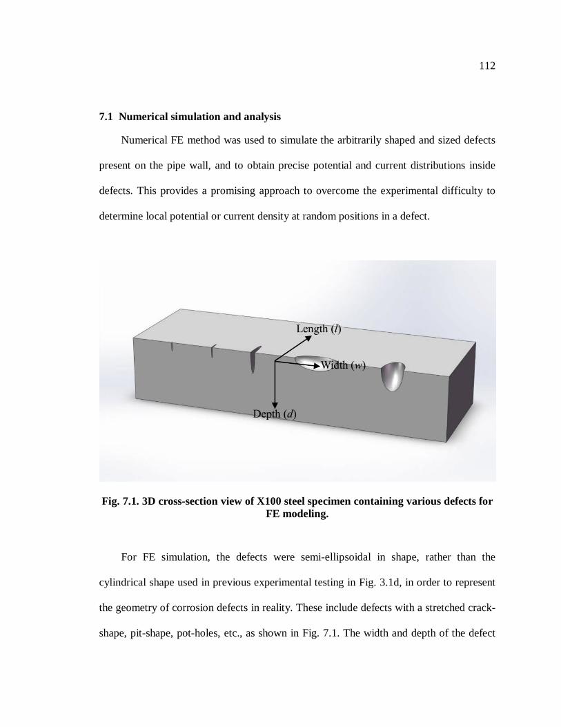
112

7.1 Numerical simulation and analysis

Numerical FE method was used to simulate the arbitrarily shaped and sized defects

present on the pipe wall, and to obtain precise potential and current distributions inside

defects. This provides a promising approach to overcome the experimental difficulty to

determine local potential or current density at random positions in a defect.

Fig. 7.1. 3D cross-section view of X100 steel specimen containing various defects for FE modeling.

For FE simulation, the defects were semi-ellipsoidal in shape, rather than the

cylindrical shape used in previous experimental testing in Fig. 3.1d, in order to represent

the geometry of corrosion defects in reality. These include defects with a stretched crack-

shape, pit-shape, pot-holes, etc., as shown in Fig. 7.1. The width and depth of the defect

113

were varied from 0 to 8 mm, and the length was approximately equal to the width for

simplification during FE modelling.

The FE simulation was performed through commercial software COMSOL

Multiphysics 4.2a. Two physical fields were used in FE modelling:

(1) Field-I: Electrochemical corrosion reactions at the steel/solution interface;

(2) Field-II: Potential and current density distributions in solution and on the steel

electrode.

The mathematical equations for describing "Field-I" and "Field-II" refer to Eqs. 6.2-

6.8 and 6.13-6.14 in Chapter 6, respectively. The exchange current densities of anodic

and cathodic reactions are derived from the measured polarization curve, as shown in Fig.

6.2, through the Tafel extrapolation. The electrochemical corrosion parameters used as

the initial inputs for FE simulation are summarized in Table 6.1. The conductivities of

NS4 solution and X100 steel electrode are also identical to those contained in Chapter 6.

7.2 Results

7.2.1 Distributions of potential and current density on the steel electrode

Fig. 7.2 shows the linear distribution of potential across defects on the steel

electrode surface in NS4 solution without and with cathodic potential of -1 V(SCE)

measured experimentally by the microprobe and simulated numerically. It is seen that, in

the absence of cathodic potential, the surface potential of the steel electrode simulated by

FE is constantly at -0.72 V(SCE), while that obtained by experimental measurements

show slight fluctuations around -0.72 V(SCE). When the cathodic potential of -1 V(SCE)

is applied, the surface potential obtained by both methods fluctuates around -0.98

114

V(SCE). Furthermore, there is no apparent potential difference between defects and the

intact area. The numerical results show an excellent agreement with the experimental

data.

Fig. 7.3 shows the distribution of current density across defects on the steel

electrode under -1 V(SCE) potential in NS4 solution. Current peaks are observed above

the defect center, while the current density drops gradually to the base level on the intact

part of the electrode. The FE simulation shows a good coincidence with the experimental

measurements, especially at the defect area.

0 5 10 15 20 25 30 35 40 45 50 55 60-1.1

-1.0

-0.9

-0.8

-0.7

-0.6

-0.5

Pote

ntia

l (V,

SCE

)

Length (mm)

No CP-Experimental CP (-1 V)-Experimental No CP-FE CP (-1 V)-FE

Fig. 7.2. Linear distribution of potential across defects on X100 steel electrode surface in NS4 solution without and with CP of -1 V(SCE) measured experimentally

by the microprobe and simulated numerically.

115

0 5 10 15 20 25 30 35 40 45 50 55 600

50

100

150

200

250

300

Curre

nt d

ensit

y (µ

A/cm

2 )

Length (mm)

CP (-1 V)-Experimental CP (-1 V)-FE

3 mm 4 mm2 mm

1 mm

0.5 mm

Fig. 7.3. Distribution of current density across defects on the steel electrode under -1 V(SCE) potential in NS4 solution.

0 1 2 3 4 5 6 7 8-1.00

-0.95

-0.90

-0.85

-0.80

-0.75

Pote

ntia

l (V,

SCE

)

Depth (mm)

0.5 mm-FE 1mm-Experimental 1mm-FE 2mm-Experimental 2mm-FE 3mm-Experimental 3mm-FE 4mm-Experimental 4mm-FE

Fig. 7.4. Potential distribution inside defects with various widths in NS4 solution when the steel is under -1 V(SCE) CP potential.

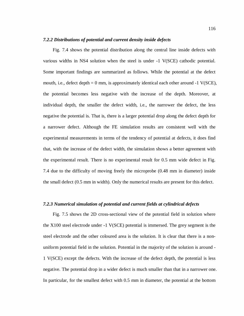
116

7.2.2 Distributions of potential and current density inside defects

Fig. 7.4 shows the potential distribution along the central line inside defects with

various widths in NS4 solution when the steel is under -1 V(SCE) cathodic potential.

Some important findings are summarized as follows. While the potential at the defect

mouth, i.e., defect depth = 0 mm, is approximately identical each other around -1 V(SCE),

the potential becomes less negative with the increase of the depth. Moreover, at

individual depth, the smaller the defect width, i.e., the narrower the defect, the less

negative the potential is. That is, there is a larger potential drop along the defect depth for

a narrower defect. Although the FE simulation results are consistent well with the

experimental measurements in terms of the tendency of potential at defects, it does find

that, with the increase of the defect width, the simulation shows a better agreement with

the experimental result. There is no experimental result for 0.5 mm wide defect in Fig.

7.4 due to the difficulty of moving freely the microprobe (0.48 mm in diameter) inside

the small defect (0.5 mm in width). Only the numerical results are present for this defect.

7.2.3 Numerical simulation of potential and current fields at cylindrical defects

Fig. 7.5 shows the 2D cross-sectional view of the potential field in solution where

the X100 steel electrode under -1 V(SCE) potential is immersed. The grey segment is the

steel electrode and the other coloured area is the solution. It is clear that there is a non-

uniform potential field in the solution. Potential in the majority of the solution is around -

1 V(SCE) except the defects. With the increase of the defect depth, the potential is less

negative. The potential drop in a wider defect is much smaller than that in a narrower one.

In particular, for the smallest defect with 0.5 mm in diameter, the potential at the bottom

117

is -0.78 V(SCE) only, while that at the defect mouth is about -1 V(SCE), a 0.22 V

difference over the depth of 8 mm. For the largest defect with 4 mm in diameter, the

potential difference between the defect mouth and its bottom (approximately -0.9 V(SCE))

is about 0.1 V only.

Fig. 7.5. 2D cross-sectional view of the potential field in solution where the X100 steel electrode under -1 V(SCE) potential is immersed (unit: V).

Fig. 7.6 shows the 3D view of the distributions of potential and Fe dissolution

current density when the steel electrode is under -1 V(SCE) in NS4 solution. As seen in

Fig. 7.6a, the potential on the electrode surface is -1 V(SCE), while that at defect

becomes less negative. There is the least negative potential at the defect bottom.

Moreover, with the increase of the defect width, the potential drop at the defect becomes

smaller. Furthermore, with application of -1 V(SCE), the steel corrosion outside defects

can be mitigated effectively, as indicated by the dissolution current density of zero in Fig.

118

7.6b. However, due to the non-uniform distribution of cathodic potential at defects, the

defected area cannot be protected properly. For small defects with 0.5 mm and 1 mm in

diameter, the Fe dissolution current density at the defect bottom is quite high. For larger

defects, the dissolution of steel inside defects is marginal due to permeation of CP into

the defect, as shown in Fig. 7.5.

Fig. 7.6. 3D view of distributions of potential (a. unit: V) and Fe dissolution current density (b. unit: µA/cm2) when the steel electrode is under -1 V(SCE) in NS4

solution.

(a)

(b)

119

7.2.4 Numerical simulation of potential and current fields at ellipsoidal defects

To represent the corrosion defects generated on pipelines in reality, ellipsoid-shaped

defects are simulated numerically by FE modeling in Fig. 7.7, where the 2D potential

distribution at defects with varied depths and widths under -1 V(SCE) in NS4 solution is

present. Identical to the potential distribution at cylindrical defects, there is a more

negative potential outside the defect and less negative potential inside. This becomes

more obvious with the increasing defect depth and the decreasing width.

Both experimental testing and numerical simulation show that the bottom of the

corrosion defect is always associated with the least negative potential when pipeline is

under a CP potential, and thus, presents the least protective location. The CP performance

at the defect bottom is critical to service life of pipelines. Further simulations of cathodic

potential and anodic/cathodic current densities at the defect bottom are shown as follows.

Fig. 7.8 shows the local potential at corrosion defects with various widths and

depths on X100 steel under -1 V(SCE) in NS4 solution. It is seen that, with the increase

of the defect depth, the potential becomes less negative. Moreover, the wider the defect,

the easier the CP penetrates into the defect. In particular, when defect is smaller than 0.01

mm in width, almost all CP is shielded, and the potential at the defect bottom is close to -

0.72 V(SCE), i.e., corrosion potential of X100 steel in NS4 solution. Even for large

defects, CP can be partially shielded from penetration. Thus, CP would lose its

effectiveness, at least partially, at corrosion defects, especially for narrow, deep ones.

120

Fig. 7.7. 2D potential distribution at ellipsoid-shape defects with various depth (d) and width (w) under CP of -1 V (SCE) in NS4 solution (unit: mm).

0 1 2 3 4 5 6 7 8 9 10-1.00

-0.95

-0.90

-0.85

-0.80

-0.75

-0.70

Pote

ntia

l (V,

SCE

)

Defect depth (mm)

0.001 0.01 0.1 0.5 1 1.5 2 3 4 5 6 7 8

Defect width (mm)

Fig. 7.8. Local potential at corrosion defects with various widths and depths on X100 steel under -1 V(SCE) in NS4 solution.

121

0 1 2 3 4 5 6 7 8 9 100.0

0.5

1.0

1.5

2.0

2.5

3.0

3.5

4.0

Fe d

issol

utio

n cu

rrent

den

sity

(µA/

cm2 )

Defect depth (mm)

0.001 0.01 0.1 0.5 1 1.5 2 3 4 5 6 7 8

Defect width (mm)

Fig. 7.9. Fe dissolution current density at corrosion defects with various widths and depths on X100 steel under -1 V(SCE) in NS4 solution.

Fig. 7.9 shows the Fe dissolution current density at corrosion defects with various

widths and depths on X100 steel under -1 V(SCE) in NS4 solution. It is seen that the

current density is zero at the defect mouth, indicating that the steel is fully protected by

CP. However, with the increase of the depth, there is an increasing dissolution current

density, showing that CP loses its effectiveness somewhat inside the defect. For wide

defects, the current density increase is not remarkable. A significant increase of Fe

dissolution current density is observed for narrow defects, such as those with 0.001-0.1

mm in width.

122

0 1 2 3 4 5 6 7 8 9 100

-10

-20

-30

-40

-50

-60

-70

-80

H ev

olut

ion

curre

nt d

ensit

y (µ

A/cm

2 )

Defect depth (mm)

0.001 0.01 0.1 0.5 1 1.5 2 3 4 5 6 7 8

Defect width (mm)

Fig. 7.10. Hydrogen evolution current density at defects with various widths and depths on X100 steel under -1 V(SCE) in NS4 solution.

Fig. 7.10 shows the hydrogen evolution current density at defects with various

widths and depths on X100 steel under -1 V(SCE) in NS4 solution. It is seen that the

cathodic current density decreases with the increasing defect depth. While the cathodic

current density is about 75 μA/cm2 at the defect mouth where the steel is under -1

V(SCE), the current density at the bottom of the defect that are narrower than 0.1 mm is

about 3.5 µA/cm2 only. Moreover, the wider the defect, the easier the cathodic current

density reaches the defect bottom.

123

7.2.5 Numerical simulation of potential and current fields at ellipsoidal defects under various applied cathodic potentials

Fig. 7.11 shows the potential at the bottom of the defect with 4 mm depth and

various widths as a function of applied cathodic potential in NS4 solution. It is seen that,

for wide defects, such as those with the mouth width more than 1 mm, there is an

approximately linear relationship between the applied potential and the potential at the

defect bottom. Particularly, the wider the defect, the more consistent of the potential at

defect bottom with the applied value, indicating that the applied CP can reach the defect

bottom completely. However, for narrow defects, such as those with the mouth width less

than 1 mm, the applied cathodic potential is shielded partially or even completely by the

defect geometry. For example, when the defect width is 0.01 and 0.001 mm, the potential

at the defect bottom is still -0.72 V(SCE) even the cathodic potential applied is as

negative as -1.1 V(SCE).

Fig. 7.12 shows the Fe dissolution current density at the bottom of defects with 4

mm depth and various widths as a function of applied cathodic potential in NS4 solution.

It is seen that, with the increase of applied CP potential, the Fe dissolution current density

at the defect bottom drops to almost zero for wide defects. However, for 0.001 mm and

0.01 mm wide defects, there is little change even when the cathodic potential is as

negative as -1.1 V(SCE). Apparently, the CP potential is shielded at narrow defects.

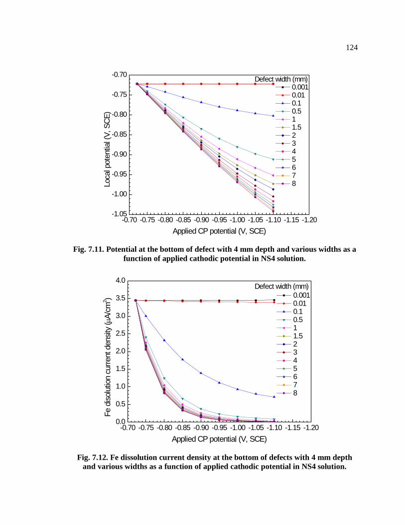
124

-0.70 -0.75 -0.80 -0.85 -0.90 -0.95 -1.00 -1.05 -1.10 -1.15 -1.20-1.05

-1.00

-0.95

-0.90

-0.85

-0.80

-0.75

-0.70

Loca

l pot

entia

l (V,

SCE

)

Applied CP potential (V, SCE)

0.001 0.01 0.1 0.5 1 1.5 2 3 4 5 6 7 8

Defect width (mm)

Fig. 7.11. Potential at the bottom of defect with 4 mm depth and various widths as a function of applied cathodic potential in NS4 solution.

-0.70 -0.75 -0.80 -0.85 -0.90 -0.95 -1.00 -1.05 -1.10 -1.15 -1.200.0

0.5

1.0

1.5

2.0

2.5

3.0

3.5

4.0

Fe d

isolu

tion

curre

nt d

ensit

y (µ

A/cm

2 )

Applied CP potential (V, SCE)

0.001 0.01 0.1 0.5 1 1.5 2 3 4 5 6 7 8

Defect width (mm)

Fig. 7.12. Fe dissolution current density at the bottom of defects with 4 mm depth and various widths as a function of applied cathodic potential in NS4 solution.

125

-0.70 -0.75 -0.80 -0.85 -0.90 -0.95 -1.00 -1.05 -1.10 -1.15 -1.200

-20

-40

-60

-80

-100

-120

-140

H ev

olut

ion

curre

nt d

ensit

y (µ

A/cm

2 )

Applied CP potential (V, SCE)

0.001 0.01 0.1 0.5 1 1.5 2 3 4 5 6 7 8

Defect width (mm)

Fig. 7.13. Hydrogen evolution current density at the bottom of defects with 4 mm depth and various widths as a function of applied cathodic potential in NS4 solution.

Fig. 7.13 shows the hydrogen evolution current density at the bottom of defects with

4 mm depth and various widths as a function of applied cathodic potential in NS4

solution. It is seen that, generally, the hydrogen evolution current density increases

negatively with the applied cathodic potential. The wider the defect, the faster the

cathodic current density increases. However, there is no visible change of hydrogen

evolution current density for narrow defects, such as those with 0.001 mm and 0.01 mm

in width, even when cathodic potential is up to -1.1 V(SCE).

126

7.3 Discussion

7.3.1 Error analysis of the experimental and numerical results

The FE numerical simulation is used in this work to overcome the experimental

difficulty to measure directly the potential and current density distributions at small

corrosion defects, such as those with width less than 0.5 mm, on pipelines. Moreover, the

FE modelling enables simulation of anodic and cathodic current densities, rather than a

net current density measured by SVET, at the defects, and thus provision of more

mechanistic information.

The present work shows that the FE simulation data is well consistent with the

experimental results, as seen in Figs. 7.2-7.4. However, we do find that the results

obtained from the two methods do not fully coincide with each other. This phenomenon

is attributed to experimental errors and simplification in FE modelling.

(1) Measurement errors. It is appreciated that a finer microprobe could achieve a

higher measurement resolution. However, no matter what the size of the microprobe is,

the measured value is actually an averaged result over a certain area, rather than that at a

specific point. Contrarily, the FE simulation is able to provide point-to-point values.

(2) Ohmic potential drop. When a microprobe is close to the surface of a target

electrode or moves into a defect, the in-situ solution is occupied by the probe. This can

disturb the current flow path from counter electrode to the target electrode. Consequently,

the local potential and current density distributions are disturbed at a somewhat level.

Particularly, when the microprobe goes into a small, deep defect, the disturbance is not

ignorable. The smaller the defect, the more significant the disturbance will be. Therefore,

the agreement between the experimental results and FE data becomes better with the

127

increasing defect width, as seen in Fig. 7.4.

(3) Interference of corrosion product. Upon CP application, a non-uniform

distribution of cathodic potential causes corrosion to occur locally, such as at the bottom

of a small, deep defect. Corrosion product would generate and deposit, affecting the

potential and current density distributions. Moreover, the hydrogen evolution generates

bubbles adhering to the steel surface, which can also affect the potential and current

distributions. These factors have not been considered in FE modelling.

Apparently, there exists a deviation between the experimental and numerical results.

However, this deviation is not appreciable as demonstrated in this work, and would not

affect corrosion analysis at a non-acceptable tolerance. Therefore, the FE modelling is a

reliable, flexible approach to investigate corrosion and the CP effectiveness at defects,

and provides information that is quite difficult or impossible to obtain from experimental

testing.

7.3.2 Effect of defect geometry on potential distribution

The present work confirms both experimentally and numerically that the local

potential distribution can be affected remarkably by the presence of corrosion defect on

steel that is under a CP potential. While the steel surface is under a full CP, the potential

at the defect, especially at the defect bottom, tends to be less negative. For wide and

shallow defects, the potential drop between the defect mouth and its bottom is small, and

the defect is thus associated with an effective CP. However, for narrow and deep defects,

such as corrosion pits and cracks, the applied CP can be shielded partially or even

completely. For example, for defects less than 0.01 mm in width and more than 3 mm in

128

depth, the potential at the defect bottom is much less negative than the applied CP

potential, as seen in Fig. 7.11. Thus, although the steel is under a full CP for corrosion

protection, the defect can still experience significant corrosion at its bottom.

Fig. 7.14. Conceptual model is developed to illustrate mechanistically generation of a potential drop in defect.

A conceptual model is developed to illustrate mechanistically the generation of a

potential drop in defect in Fig. 7.14, where the solution resistance effect and cathodic

current dissipation effect are discussed for this purpose.

(1) Solution resistance effect. Solution resistance in a defect results in a potential

drop upon flow of cathodic current. Generally, the solution resistance in a defect is a

function of solution conductivity and the defect geometry. The solution inside the defect

is modelled as n cells in series connection, with each in length dl. When n→∞, dl→0.

Integral method is employed to calculate of the solution resistance, R, by [121, 126, 127]:

φB

Δφ = φB- φS CP Current dissipation

along defect

Defect depth

Potential drop Δφ

φS

129

∑ ∑ ∫= =

===n

i

n

i ii

ii dl

AAdl

RR1 1

1σσ

(7.1)

where dli, σi and Ai are length, conductivity and area of the cell i, respectively. In

experimental testing, the defect is cylindrically shaped. The solution resistance inside

defect is simply calculated as [121, 126, 127]:

ALRcylinder σ

= (7.2)

where L is the defect depth of 8 mm, and A is cross-section area of the defect cylinder.

In FE simulation, the defect is in a semi-ellipsoidal shape, and the solution

resistance inside defect is derived from Eq. (7.1):

zdzddwdz

zdwldR

d

ellipsoid −+

=−

= ∫ ln8

14

2

0 22

2

σπ

σπ (7.3)

where w, l and d are semi-principal axes of the width, length and depth of a semi-

ellipsoidal defect as shown in Fig. 7.1 (w, l, d > 0), respectively. The value of z is less

than d in FE calculation.

According to Eqs. (7.2) and (7.3), a decrease of the defect width and an increase of

the defect depth would cause the increase in solution resistance. Consequently, a high

130

potential drop Δφ is generated when cathodic current flows into the defect, as seen in

Figs. 7.5, 7.8 and 7.11, by Ohm's law:

SBIR ϕϕϕ −==∆ (7.4)

where superscripts B and S refer to the defect bottom and the surface of steel electrode,

respectively, and I is total current flowing into the defect upon application of a cathodic

potential. Δφ is a non-negative variable.

(2) Cathodic current dissipation effect. Since the defect wall is not electrically

isolated, the current dissipation effect should be taken into consideration as a factor

contributing to potential drop in the defect. Under a given voltage, there is usually more

current flowing along path with a lower electric resistance [121]. Therefore, when

cathodic current flows into a defect, it goes to the nearest wall and then flows to the

bottom, resulting in a dissipation of current from the defect mouth to its bottom. This is

proven by the FE simulation, as indicated by the direction and intensity of red arrows

distributed in the defect in Fig. 7.14. Thus, the current, I, in Eq. (7.4) is a variable, rather

than a constant. A nonlinear dependence of potential drop on the defect depth and width

is expected, as shown in Fig. 7.8.

7.3.3 Effect of defect geometry on current density distribution

As demonstrated, the anodic and cathodic current densities at the steel/solution

interface and the net current density in solution are not uniform. The SVET is capable of

measuring the net current density only. The local anodic and cathodic current densities

131

are not measureable directly. Moreover, the measured SVET current density is confined

to the electrode surface (Fig. 7.3), and the current density at the defect is not measurable

due to the limited size of the defect. Indeed, the FE modelling shows its promising ability

to obtain the cathodic and anodic partial current densities inside defects.

It is worth noting that, during SVET measurements on the steel electrode surface,

the current density peak does not decrease with the increasing defect width, as shown in

Fig. 7.3, which seems inconsistent with the results shown in Fig. 7.4. This is actually

caused by the distance of 200 µm between the steel electrode and the SVET probe.

Obviously, the current density measured by SVET probe which is located above the

electrode surface is incapable of reflecting the profile of current density inside a defect.

The anodic and cathodic partial current densities are more essential to understand

the corrosion process. Anodic current density refers to the dissolution rate of steel, and

the cathodic current density indicates the hydrogen evolution rate in this work. According

to Eqs. (6.4)-(6.6) in Chapter 6, the anodic and cathodic current densities are determined

by overpotential of the individual reactions. The more negative the electrode potential,

the smaller the Fe dissolution current density and the higher the hydrogen evolution

current density. As shown in Figs. 7.9 and 7.10, under a given cathodic potential of -1

V(SCE), there is a higher Fe dissolution current density and lower hydrogen evolution

current density as the defect depth increases or its width decreases. At a certain defect

depth, a more negative cathodic potential would mitigate the Fe dissolution and increase

the hydrogen evolution at the defect bottom.

Furthermore, the CP effectiveness inside a defect decreases as its width decreases,

especially for those narrow defects, e.g., 0.001 mm and 0.01 mm in width, as seen in Figs.

132

7.10–7.13. It is expected that different corrosion scenarios would be experienced outside

and inside defects on pipelines. When a sufficiently negative CP potential is applied, the

steel is under a full protection, but the hydrogen evolution is not ignorable. Hydrogen

embrittlement constitutes a potential threat to integrity of the steel pipes. However, there

is a lower risk of hydrogen embrittlement inside corrosion defects, especially for those

with a larger depth and smaller width. This is attributed to the solution resistance effect

and cathodic current dissipation effect existing in the defect. However, the enhanced

dissolution of steel at the defect bottom due to ineffective CP would result in localized

corrosion, particularly pitting corrosion, potentially resulting in pipeline leaking.

7.3.4 Implications on CP performance on pipelines and defect assessment

This work demonstrates that CP would not be able to provide an effective protection

at defects, which include mechanical dents, corrosion pits and micro-cracks, on pipelines.

In reality, monitoring of CP potential is conducted on the pipeline surface only. A real-

time measurement of the potential distribution inside defects is unavailable and also

unrealistic in industry. Without this information, it is impossible to ensure pipelines under

a full protection by CP. For industrial application, an empirical equation is developed,

based on FE simulation and the experimental validation, in order to determine the

potential drop along an arbitrarily geometrical defect:

( )

+

−−−−=∆1ln

exp)()( nCPcorrCPcorr wd

ασϕϕϕϕϕ (7.5)

133

where φcorr is corrosion potential (V) of steel, φCP is applied CP potential (V) with the

same value as φS in Eq. (7.4), d is the defect depth (mm), w is width of defect (mm), σ is

conductivity of soil (S/m), α is a correction factor (m/S), and n is a geometrical

coefficient (dimensionless), which equals to π/4 for ellipsoid-shaped defects, and 1 for

cylindrical defects. By substituting Eq. (7.5) into Eq. (7.4), the local potential inside the

defect and at the defect bottom can be calculated.

Since the remaining service life of pipelines depends primarily on the propagation

rate of corrosion defects along the radial direction, the corrosion rate at the defect bottom

is thus crucial for risk assessment of pipelines if the defect propagation is dissolution-

controlled, a typical situation resulting in pipeline leaking by pitting corrosion. According

to Eqs. (6.4), (6.6), (7.4) and (7.5), an equation is derived to calculate the ratio, ν, of

corrosion rate of the defect bottom to that of the steel surface:

aa

SB

a

SB

a

Sa

a

Ba

bbb

baeq

baeq

Sa

Ba

i

iii ϕϕϕηη

η

η

ν∆−−

===== 10101010

10 )()(

0,

0, (7.6)

For a defect with 0.1 mm in width and 2 mm in depth on X100 steel pipe surface

where a -1 V(SCE) cathodic potential is applied, the ratio is calculated as 26, indicating

that the corrosion rate at the defect bottom is approximately 26 times of that of the steel

surface.

134

Furthermore, considering that the cathodic current density is much higher than the

anodic one under CP, the percentage of current dissipation along a defect can be

approximately calculated by:

Cathodic current dissipation = %100101%1001 ×

−=×

−

∆cb

Sc

Bc

ii ϕ

(7.7)

where icB and ic

S are cathodic current densities at the defect bottom and the steel surface,

respectively, and bc is cathodic Tafel slope. For situation given above, the percentage of

cathodic current dissipation along the defect is up to 84%. In other words, only 16% of

CP current reaches the defect bottom for corrosion mitigation. Moreover, the current

dissipation effect increases significantly with the increasing defect depth and/or

decreasing defect width.

The derived empirical equations (7.5)-(7.7) can be conveniently used to determine

the local potential and anodic/cathodic current densities at defects, and enable assessment

of the CP effectiveness on pipelines in the presence of various geometrical defects. It is

thus capable of estimating the further corrosion allowance and remaining service life of

pipelines in the field.

Moreover, it is inferred from this work that the existing defects would prefer to

propagate along the depth direction, rather than the width one, due to the highest

corrosion rate at the bottom. This corrosion scenario would accelerate propagation of

defects along the radial direction of pipelines together with other synergistic effects such

as stress concentration, stress enhanced corrosion, etc. Therefore, the narrow, deep

135

defects are always associated with much higher failure risk than those with a wide,

shallow geometry. In the routine maintenance these types of defects present on the pipe

wall need an extra attention. Removal mechanically and re-coating or sleeving are

preferential measures to ensure reliable operation of pipelines.

7.4 Summary

While CP is applied on pipelines for corrosion prevention, there are non-uniform

potential and current density distributions at corrosion defects present on the pipe surface.

A potential drop can be developed inside the defect due to both the solution resistance

effect and the current dissipation effect. As a consequence, the CP potential applied

would be shielded, at least partially, at the defect bottom, reducing the effectiveness of

CP for corrosion protection. This effect depends on the defect geometry, and is enhanced

with an increase in defect depth and decrease of its width.

Empirical equations are derived to enable determination of the potential drop inside

defect, and thus the potential and current density distributions in the defect, especially at

the defect bottom, while CP is applied on the pipeline. They are capable of assessing

conveniently for industry the CP effectiveness at defects and the further corrosion

scenario on pipelines.

Numerical modelling based on the FE simulation provides a promising alternative

which overcomes the experimental difficulty and is capable of determining local potential

and current density as well as CP effectiveness at defects on pipelines, enabling

assessment of further corrosion allowance and remaining service life of pipelines in the

field.

136

Chapter Eight: Prediction of failure pressure of pipelines under synergistic effects of internal pressure, soil strain and corrosion defects

The remaining strength of pipeline steels in the field depends on a number of factors,

including the operational conditions, mechanical damage, corrosion, ground movement,

etc. In particular, corrosion is of concern because any loss of the pipe wall thickness

means a reduction of the structural intensity and hence an increase in the risk of failure.

Moreover, the ground movement produces a longitudinal stress/strain on the pipe to

threaten its safety. A synergistic effect of operating pressure, corrosion and the soil strain

on the pipeline integrity should be considered in evaluation and prediction of failure

pressure of pipelines.

Generally, a pipeline containing corrosion defect is allowed to operate after the

reliability assessment to recalculate its maximum allowable operating pressure. Standards

and codes have been developed to estimate the remaining strength of pipelines by

calculating the failure pressure in the presence of local corrosion defects [16, 72, 80, 128].

Particularly, American Society of Mechanical Engineers (ASME) B31G standard [14],

which was originally developed and published in 1984, has been used widely to

determine the remaining strength of the corroded pipeline. Moreover, a computer code

named “modified B31G” is also used [76, 77]. The DNV-RP-F101 describes another

method to evaluate the reliability of corroded pipelines under complex conditions, e.g.,

corrosion-induced defects, internal pressure, and the longitudinal compressive and

bending loads due to soil movement [15]. These three models are named “industry

137

models” in the following text representing the available methodology for determination

of failure pressure of pipelines.

With the development of new, high-strength steel pipelines in remote geographic

terrains, the industry models do not give accurate results for the failure pressure

prediction due to a number of reasons. These models were developed to address

reliability assessment for pipelines that were made of low grades of steel, such as those

with grade lower than X80, and contained corrosion defects with a smooth and regular

shape. Moreover, the synergism of local stress/strain concentration and corrosion reaction

was usually ignored. The field experiences have demonstrated that the available industry

models become non-applicable on high-strength steel pipelines.

In this chapter, a FE model, named UC model, was developed to predict the failure

pressure of pipelines with considerations of the synergism of internal pressure, soil strain

and corrosion defect. As a comparison, the relevant calculations and analysis were

conducted on the three industry models to evaluate their applicability on pipelines made

of high grades of steel and contain defects with various depths. The deviation of the

predicted failure pressure by these models was compared to the newly developed UC

model. The tested steels included various strength levels, such as X65, X80 and X100

steels. The results provide recommendations to industry for safe, reliable operation of

pipelines under a reasonable internal pressure.

138

8.1 Models for reliability assessment and failure pressure prediction of pipelines

8.1.1 Present industry models

The ASME B31G model was developed based on full-scale burst tests of corroded

pipes [14]. Application of this model is limited to evaluation of the metal wall loss due to

external or internal corrosion, where the corrosion defects have a smooth contour with the

depth between 10% and 80% of the pipe wall thickness. Crack-like defects, grooving

corrosion, selective corrosion, and preferential corrosion affecting pipe seams or girth

welds are excluded. According to this mode, the failure pressure and flow stress of pipe

steel with defects are determined as:

2/1)8.01( zM += (8.1)

For z ≤ 20,

⋅

−

−

=

Mtd

td

DtP flowF 1

321

321

2σ (8.2)

For z > 20,

−=

td

DtP flowF 12σ (8.3)

SMYSflow ⋅= 1.1σ (8.4)

139

where PF is the estimated failure pressure of pipeline, flowσ is flow stress, D is outer

diameter of the pipe, t is the pipe wall thickness, d is depth of corrosion defect, z = L2/Dt

and L is the length of corrosion defect, SMYS is specified minimum yield strength of

pipe steel, and M is a constant. The original B31G equation used for high-strength

materials by Eq. (8.4) is not applicable to high grades of pipeline steel, such as X100

steel. The B31G actually defines the burst pressure in terms of σflow, and contains several

possible definitions and ranges of applicability for the flow stress equation.

The modified B31G model was derived from ASME B31G model with

modifications of effective corrosion area and flow stress, shown as follows [76, 77].

For z ≤ 50,

2/12 )003375.06275.01( zzM −+= (8.5)

For z > 50,

3.3032.0 += zM (8.6)

⋅

−

−

=

Mtd

td

DtP flowF 185.01

85.012σ (8.7)

MPaSMYSflow 69+=σ (8.8)

The DVN-RP-F101 model is capable of assessing pipelines containing a single

defect, multiple interacting defects and complex shaped defects as well as a single defect

under the combined internal pressure and the longitudinal compressive stress [15]. For an

140

isolated corrosion defect under pipeline internal pressure and the defect depth not

exceeding 85% of the wall thickness:

2/12

)31.01(DtLM += (8.9)

⋅

−

−

−=

Mtd

td

tDtP flowF 11

12σ (8.10)

where flowσ = SMTS, SMTS is the specified minimum tensile strength of pipe steel.

The three industry models were developed to predict failure pressure of pipelines

that are made of low grades of steel, such as those with grade lower than X80. Moreover,

the corrosion defect was assumed regularly shapped. The synergistic effect of internal

pressure, soil strain (tensile in particular) and local stress concentration at corrosion

defect is not considered in the prediction. Thus, the delivered results are not accurate with

the actual situation, as demonstrated from the field experiences.

8.1.2 FE modeling assessment

The developed FE-based UC model is based on simultaneous considerations of

multiple factors, including operating pressure, soil strain and corrosion defects with

varied geometries, in prediction of failure pressure of pipelines. The FE modeling

assessment was carried out using COMSOL Multiphysics software, and a non-linear

elasto-plastic model was applied for simulating the mechanical behavior, i.e., the elastic

141

and plastic deformation and burst pressure, of the steel. The possible data fitting was

performed during the FE calculation. In material’s elasto-plastic setting, the isotropic

hardening model was chosen and the hardening function was defined as [118]:

yse

pyseffyhard Eσσεσσεσσ −+=−= )()( expexp (8.11)

where σexp is the experimental stress function, εeff is the total effective strain, εp is the sum

of the plastic strain, σe is the effective stress, σys is the yield stress, and E is Young’s

modulus. Some important settings in FE included:

(1) Element type: Lagrange-quadratic;

(2) Analysis type: Static, elasto-plastic;

(3) Solver: direct (Spooles);

(4) Mesh parameter: 5mm in the defect;

(5) von Mises yield criterion was used.

8.1.3 The FE simulation

Three grades of pipe steel and four corrosion depths were chosen for the FE

modeling. The details of the mechanical properties of the steels and the geometries of the

corrosion defect are shown in Tables 8.1–8.3. It is realized that, in reality, the aspect ratio

of a corrosion defect would change when its depth increases. This work assumes

unchanged length and width with the growing depth of the corrosion defect along the

wall thickness direction. Fig. 8.1 shows the typical stress-strain curves of three types of

142

pipe steel. Due to the symmetrical geometry of the pipe, a quarter model was used for the

FE simulation, as shown in Fig. 8.2. The corrosion defect was treated as elliptical shape.

Table 8.1. Mechanical properties of various grades of pipeline steel.

Mechanics properties X65 steel X80 steel X100 steel

Young's modulus (MPa) 207000 207000 207000

Poisson's ratio 0.3 0.3 0.3

SMYS (MPa) 456 646 803

SMTS (MPa) 570 760 891

Yield/Tensile strength (Y/T) 0.80 0.85 0.90

Table 8.2. Geometry of line pipe for the FE simulation.

Pipe Length (m) Outer Diameter (m) Wall thickness (m)

2 812.8×10-3 19.1×10-3

Table 8.3. Geometry of corrosion defects investigated in this work

Length of defect (mm) 200

d1 (mm), 20% of wall thickness 3.82

d2 (mm), 40% of wall thickness 7.64

d3 (mm), 60% of wall thickness 11.46

d4 (mm), 80% of wall thickness 15.28

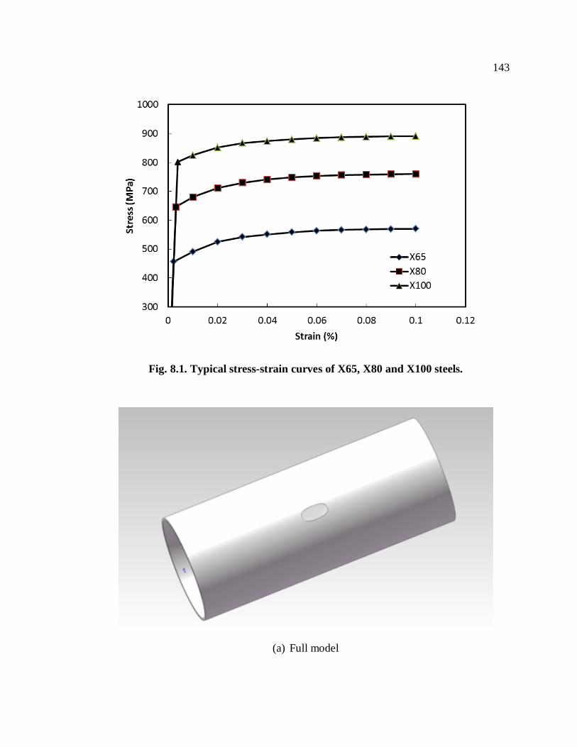
143

Fig. 8.1. Typical stress-strain curves of X65, X80 and X100 steels.

(a) Full model

144

(b) Quarter model

Fig. 8.2. 3-D modeling of the pipe with a corrosion defect: (a) full model (b) a quarter model.

8.2 Results

8.2.1 Prediction of failure pressure of pipelines by individual models

The failure pressures of the pipe steel (X65, X80 and X100 steels) containing a

corrosion defect with various depths shown in Table 8.3 determined by the industry

models and the developed UC model are shown in Tables 8.4–8.7, respectively. It is seen

that, at individual defect depth, the failure pressure of the steel pipe predicted by all

models increases with the increasing grade of steel. It is attributed to the enhanced yield

strength and ultimate tensile strength of a high grade of steel to provide a greater

resistance to deformation and rupture in the defected area. Furthermore, the failure

pressure obtained by the UC model is higher than those from the industry models. In

particular, the DNV model generates the result close to that by UC, while the ASME

145

B31G and the modified B31G models generate similar results. Compared to the UC

results, the ASME B31G model result is the highest, especially for small defects.

With the corrosion defect depth increasing to 40% of the wall thickness, the failure

pressure obtained by the DNV model becomes higher than that of the UC model, and the

results by other two models are still lower than what the UC model gives. With the

further increase of the defect depth to 60% of the wall thickness, the failure pressures by

DNV model are higher than that by UC model, while the ASME B31G and the modified

B31G models predict results higher than that of the UC for high grades of steel, i.e., X80

and X100 steels.

Table 8.7 shows the predicted failure pressures when the defect is up to 80% of the

wall thickness. Most of the results predicted by the industry models are higher than those

of the UC model, except the modified B31G and DNV models for X65 steel. The ASME

B31G predicts the highest failure pressure for X100 steel.

Table 8.4. Failure pressure of the steel pipe with a corrosion defect of 20% of pipe wall thickness and 200 mm in length determined by the individual models

Model Failure pressure (MPa)

X65 steel X80 steel X100 steel

ASME B31G 22.1 31.3 38.9

Modified B31G 22.9 31.2 38.0

DNV-RP-F101 25.8 34.4 40.3

FE 26.1 35.0 42.2

146

Table 8.5. Failure pressure of the steel pipe with a corrosion defect of 40% of pipe wall thickness and 200 mm in length determined by the individual models

Model Failure pressure (MPa)

X65 steel X80 steel X100 steel

ASME B31G 20.4 28.9 35.9

Modified B31G 20.6 28.1 34.2

DNV-RP-F101 23.5 31.3 36.7

FE 23.0 29.3 36.0

Table 8.6. Failure pressure of the steel pipe with a corrosion defect of 60% of pipe wall thickness and 200 mm in length determined by the individual models

Model Failure pressure (MPa)

X65 steel X80 steel X100 steel

ASME B31G 18.0 26.0 32.3

Modified B31G 17.7 24.1 29.4

DNV-RP-F101 19.9 26.5 31.0

FE 18.9 24.0 28.8

Table 8.7. Failure pressure of the steel pipe with a corrosion defect of 80% of pipe wall thickness and 200 mm in length determined by the individual models

Model Failure pressure (MPa)

X65 steel X80 steel X100 steel

ASME B31G 15.8 22.4 27.8

Modified B31G 13.7 18.1 22.7

DNV-RP-F101 13.6 18.1 21.3

FE 13.9 18.0 20.2

147

To quantify the relative error (RE) of the industry models in prediction of failure

pressure, the results obtained by the UC model are used as references, and the parameter

RE is defined as follows:

) ( ) (

ModelFEpressureFailureModelIndustrypressureFailureRE = (8.12)

When RE > 1, the failure pressure is overestimated; and the larger the value of RE,

the more overestimation is. If RE < 1, the failure pressure is underestimated. The smaller

the RE, the higher the prediction will be than the FE result.

Figs. 8.3–8.5 show the RE as a function of the defect depth determined by industry

models for X65, X80 and X100 steels, respectively. It is seen from Fig. 8.3 that the RE

values of both ASME B31G and the modified B31G models increase with the increasing

corrosion depth for X65 steel. The RE of ASME B31G model increases from 0.85

(underestimated failure pressure) to 1.13 (overestimated) when the defect depth increases

from 4 mm to 15 mm. The RE of the modified B31G model increases slightly from 0.88

to 0.97, indicating the underestimated failure pressure. The DNV results are around 1,

indicating that the predicted failure pressure by DNV is in good agreement with that by

the UC model.

148

Fig. 8.3. Effect of the defect depth on RE determined by industry models for X65 steel.

Fig. 8.4. Effect of the defect depth on RE of the industry models for X80 steel.

Modified B31G

Modified B31G

149

Fig. 8.5. Effect of the corrosion depth on RE of the industry models for X100 steel.

With the increase of the grade of steel to X80 and X100, as shown in Figs. 8.4 and

8.5, the RE values of ASME B31G and the modified B31G models increase with the

increasing corrosion depth, indicating that the two models tend to overestimate the failure

pressure of pipelines, and the conservatism decreases. Moreover, the RE of the ASME

B31G increases up to 1.25 for X80 steel and 1.39 for X100 steel, which are much higher

than those of the DNV, showing a significant overestimation of the model. The RE of the

DNV model fluctuates between 1 and 1.1 for all steels, indicating that there is little effect

of the steel grade on the DNV prediction.

Furthermore, the standard deviation of RE is calculated to analyze the stability of

the prediction by individual model. A low standard deviation indicates that the prediction

is stable to resist the change of external conditions, such as corrosion depth and the grade

Modified B31G

150

of the steel, and thus a high reliability of the model. Fig. 8.6 shows the standard deviation

of RE of industry models as a function of the corrosion depth. It is seen that the standard

deviation increases with the increasing corrosion depth. At the individual corrosion defect

depth, there are the largest and smallest standard deviations for the ASME B31G and

DNV models, respectively. It is further demonstrated that the B31G model tends to be

conservative, and does not provide accurate results.

Fig. 8.7 shows the standard deviation of RE of industry models for three types of

steel with different Y/T ratios. It is seen that there is the largest standard deviation for the

ASME B31G model. Although the standard deviation increases with the increasing steel

grade, the DNV model generates the most stable prediction, with a standard deviation

around 0.05.

Fig. 8.6. Standard deviation of RE of industry models under various corrosion defect depths.

Modified B31G

151

Fig. 8.7. Standard deviation of RE of industry models as a function of the steel grade.

To summarize, the three industry models for prediction of the failure pressure of

pipelines that are made of various grades of steel and contain corrosion defect are higher

than the result by the UC model for small defects, while overestimation of failure

pressure occurs with the increase of the steel grade and the corrosion defect depth.

Furthermore, the prediction reliability decreases with the increasing corrosion defect

depth and the steel grade. Compared to other two industry models, the DNV model is

relatively more reliable, and the predictive results are close to that by the UC model.

8.2.2 Determination of von Mises stress on pipelines in the presence and absence of corrosion defect

Fig. 8.8 shows the von Mises stresses determined by the UC model of the inner and

outer surfaces of an X80 steel pipe in the presence of absence of a corrosion defect with

Modified B31G

152

20% pipe wall thickness, respectively, where “outer-defect” and “inner-defect” refer to

the base of the defect present on the outer surface of the pipe and the inner pipe surface,

respectively. It is seen that, in the absence of corrosion defect, there is little difference of

von Mises stresses on the inner and outer surfaces, and the stress increases with the

internal pressure. When the corrosion defect is present, the von Mises stress at the base of

the defect is much higher than that of the inner surface of the pipe.

Fig. 8.8. Local von Mises stresses of the inner and outer surfaces of X80 steel pipe as a function of internal pressure in the presence and absence of a corrosion defect of

20% of pipe wall thickness.

When the corrosion depth is up to 80% of the pipe wall thickness, the von Mises

stress distributions on the inner and outer surfaces of the steel pipe are shown in Fig. 8.9.

It is seen that, while the von Mises stresses of the inner and outer surfaces show a linear

153

relationship with the internal pressure in the absence of defect, the von Mises stresses of

the inner and outer surfaces of the pipe with a defect are much higher than the formers.

Moreover, apparent yielding points are observed in both curves.

Fig. 8.9. Local von Mises stresses of the inner and outer surfaces of X80 steel pipe as a function of internal pressure in the presence and absence of a corrosion defect of

80% of pipe wall thickness.

Effective plastic strain is usually used to describe the intensity of plastic

deformation. Comparisons of the effective plastic strain occurring on the outer and inner

surfaces of X80 steel pipe in the absence and presence of corrosion defect are shown in

Figs. 8.10 and 8.11, respectively. It is seen that there is no plastic deformation occurring

over the measured pressure range in the absence of corrosion defect. When the corrosion

defect is shallow, i.e., 20% of the pipe wall thickness, the effective plastic strain of the

154

outer surface becomes apparent until the internal pressure exceeds 25 MPa. After that, the

plastic strain increases significantly, indicating a high plastic deformation occurring.

When the defect is up to 80% of wall thickness, the plastic deformation is

appreciable when the internal pressure is 5 MPa only. A small effective plastic strain is

observed on the inner face of the pipe as well.

According to analysis of the von Mises stress and effective plastic strain, it is seen

that there exists a stress concentration at the corrosion defect, resulting in a higher von

Mises stress than that of the inner surface of the pipe. Moreover, the deeper the defect,

the less the internal pressure is required to result in the local plastic deformation.

Fig. 8.10. Effective plastic strain of the outer and inner surfaces of X80 steel pipe in the absence and presence of a corrosion defect with 20% of pipe wall thickness.

155

Fig. 8.11. Effective plastic strain of the outer and inner surfaces of X80 steel pipe in the absence and presence of a corrosion defect with 80% of pipe wall thickness.

8.2.3 Distribution of plastic deformation and von Mises stress at corrosion defect

Figs. 8.12 and 8.13 show the front and cross-sectional views of the plastic

deformation area on a pressurized X80 steel pipe (at 18 MPa) containing a corrosion

defect with various depths, respectively. It is seen that there is no plastic deformation

zone developed when the corrosion depth is as small as 20% of the pipe wall thickness.

When the corrosion depth reaches 40% of pipe wall thickness, a plastic zone is found at

the bottom of the defect. With the further increase of the defect depth, the plastic

deformation zone spreads to the surrounding area.

156

Fig. 8.12. Front views of the plastic deformation area on a pressurized X80 steel pipe (at 18 MPa) containing a corrosion defect with different depths.

Fig. 8.13. Cross-sectional views of the plastic deformation area on a pressurized X80 steel pipe (at 18 MPa) containing a corrosion defect with different depths.

157

Fig. 8.14 shows the distribution of von Mises stress on the pressurized pipe (at 18

MPa) containing a corrosion defect with various depths. It is seen that a stress

concentration is developed at the base of the defect, and the stress intensity is enhanced

with the increasing corrosion depth.

Fig. 8.14. Distributions of von Mises stress on the pressurized pipe at 18 MPa containing a corrosion defect with various depths.

8.2.4 Effect of soil strain on plastic deformation of the corroded pipe

Pipelines experiencing significant soil-induced strains are usually named pre-

strained pipelines. The pre-strain may affect the remaining strength (failure pressure) of

pipelines containing corrosion defect. The failure pressures of X80 steel pipe containing a

corrosion defect with 80% of pipe wall thickness under applied tensile or compressive

pre-strain in longitudinal direction predicted by the UC model are shown in Tables 8.8

and 8.9, respectively, where the signs "+" and "-" indicate the tensile and compressive

158

pre-strain. It is seen that the failure pressure of the corroded pipe is reduced by the

applied pre-strain, no matter the tensile or compressive one. Moreover, the reduction in

failure pressure becomes significant with the increase of the pre-strain intensity. Under

the individual pre-strain, the failure pressure obtained under the compressive pre-strain is

higher than that obtained under a tensile pre-strain.

Table 8.8. Failure pressures of X80 steel pipe containing a corrosion defect with 80% of pipe wall loss thickness under applied tensile pre-strains in longitudinal

direction predicted by the UC model

Tensile Pre-strain 0 + 0.1% + 0.2% + 0.25% Failure pressure

(MPa) 18.0 17.0 15.3 14.4

Table 8.9. Failure pressures of X80 steel pipe containing a corrosion defect with 80% of pipe wall thickness under applied compressive pre-strains in longitudinal

direction predicted by the UC model

Compressive Pre-strain 0 - 0.1% - 0.2% - 0.25%

Failure pressure (MPa) 18.0 17.3 16.5 15.0

Fig. 8.15 shows the distribution of plastic deformation on X80 steel pipe containing

a corrosion defect with 80% of pipe wall thickness under different pre-strain conditions.

It is apparent that the plastic deformation area increases when the tensile or compressive

pre-strain is applied. However, the plastic deformation zone under the tensile strain is

quite different from that under the compressive one. The former expands along the hoop

direction and is away from the defect, while the plastic field of the latter surrounds the

defect. Therefore, a longitudinal tensile strain would result in the plastic field propagation

along the hoop direction, potentially leading to a circumferential cracking. On the

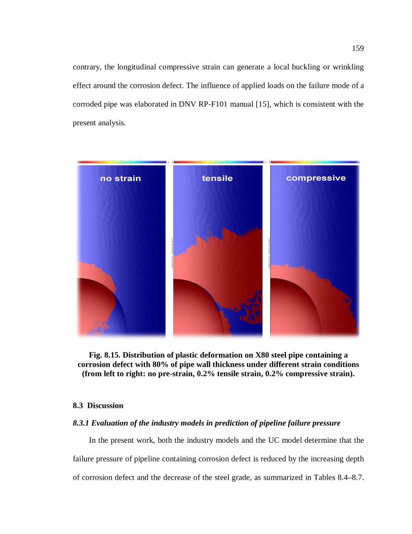
159

contrary, the longitudinal compressive strain can generate a local buckling or wrinkling

effect around the corrosion defect. The influence of applied loads on the failure mode of a

corroded pipe was elaborated in DNV RP-F101 manual [15], which is consistent with the

present analysis.

Fig. 8.15. Distribution of plastic deformation on X80 steel pipe containing a corrosion defect with 80% of pipe wall thickness under different strain conditions

(from left to right: no pre-strain, 0.2% tensile strain, 0.2% compressive strain).

8.3 Discussion

8.3.1 Evaluation of the industry models in prediction of pipeline failure pressure

In the present work, both the industry models and the UC model determine that the

failure pressure of pipeline containing corrosion defect is reduced by the increasing depth

of corrosion defect and the decrease of the steel grade, as summarized in Tables 8.4–8.7.

160

It is understandable that an increasing corrosion depth decreases the effective cross

sectional area of the pipe in the longitudinal direction, therefore, the resistance of the pipe

to failure. The increase of the steel grade, e.g., from X65 to X80 and X100 steels, the

increasing yield and tensile strengths tend to resist the plastic deformation and failure of

pipelines.

The study of relative error of the industry models relative to UC model indicates the

conservatism of the individual model in prediction of the pipeline failure pressure. This

work shows (Figs. 8.3–8.5) that the RE values of the ASME B31G and the modified

B31G models increase, and thus the conservatism of the two models decreases, with the

corrosion depth for all steels. In particular, for ASME B31G model, all RE values are

larger than 1 when the corrosion depth is up to 80% of the pipe wall thickness, indicating

that the predicted failure pressure is overestimated. An overestimation of failure pressure

is harmful to the evaluation of the remaining service life of pipelines. This situation is

further aggravated in high grade steels, such as X80 and X100 steels.

The prediction by DNV RP-F101 model is close to that obtained by the UC model.

For all the tested corrosion depths and the steel grades, the RE of DNV model is around 1,

indicating the high accuracy of the predicted failure pressure. It is thus comparable to the

UC model for failure prediction of high grade steel pipes.

The reliability of the modeling prediction is also evaluated by analysis of the

standard deviation of RE. It is clear that the predictive reliability by ASME B31G and the

modified B31G models decreases, i.e., the standard deviation increase, with the corrosion

depth and the steel grade, while the DNV model has the lowest standard deviation, as

seen in Figs. 8.6 and 8.7.

161

The ASME B31G model was proposed for the failure pressure prediction based on

validations through a large number of full-scale experimental tests of low grade pipe

steels, such as X52 and X65 steels, with small Y/T ratios. The modified B31G model was

built upon the ASME B31G by modifying the flow stress to σflow = SMYS + 69 MPa, and

the factor for the effective area of corrosion defect to 0.85, while the ASME B31G uses

σflow = 1.1 × SMYS and 2/3 as the defect area factor. The flow stress calculated by the

modified B31G model is higher and closer to the tensile strength of steel, compared to the

result calculated by the ASME B31G model. The effective area of corrosion defect is also

close to the real one used in the UC model. Thus, the modified B31G model is more

accurate than ASME B31G in the failure pressure prediction. However, it is still suitable

for low grades of steel only.

The DNV RP-F101 model was developed based on full-scale experimental tests of

high grade steels. The validation of this model includes full scale tests on steel up to X80

grade [3]. In principle, the X100 grade pipeline steel is beyond the predictive scope of the

DNV model. However, compared with the ASME B31G and the modified B31G models,

the DNV model delivers the failure pressure prediction close to that by UC model for

X100 steel, as seen in Fig. 8.7. The primary reason is that DNV model uses directly the

ultimate tensile strength as flow stress.

8.3.2 Effect of corrosion defect on stress and strain distributions on pipeline

The geometry of corrosion defect affects remarkably the local stress and strain

distributions, and thus plays a critical role in the failure pressure prediction of pipelines,

as demonstrated in this work. Generally, in the absence of corrosion defect, the von

162

Mises stress of the inner surface of pipeline is higher than that of the outer surface.

During elastic deformation of the steel, the von Mises stress along the pipe wall thickness

is determined by:

−

−= 2

2

22

2

1)(rr

rrrPr o

io

iirrσ (8.13)

+

−= 2

2

22

2

1)(rr

rrrPr o

io

iiθθσ (8.14)

22

2

)(io

iizz rr

rPr−

=σ (8.15)

2)()()()(

222rrzzzzrr

Misesvon r σσσσσσσ θθθθ −+−+−=⋅ (8.16)

where ri and ro are the inner and outer radii of the pipe, r is the distance from the central

axis to a point in the wall and ri ≤ r ≤ ro, Pi is the internal pressure, and rrσ , θθσ and

zzσ are the radial stress, hoop stress and longitudinal stress, respectively. It is seen that

the von Mises stress depends linearly with the internal pressure, as verified by the UC

results in Figs. 8.8 and 8.9. However, the equations proposed are not applicable for both

the defected area and the plastic deformation region.

The UC model provides a promising tool to calculate the stress and strain

distributions on the pipe. When the corrosion depth is small, as shown in Fig. 8.8, the von

Mises stress on the inner surface of pipe is much lower than that at the defect base, which

is attributed to the stress concentrated at the defect. With the increase of the corrosion

163

depth, the stress concentration is enhanced, resulting in the further separation of the von

Mises stresses of the inner surface and that of the defect base, as shown in Fig. 8.9.

Another interesting phenomenon is that, while the increasing corrosion depth has a

great influence on effective plastic strain of the outer surface of pipe, there is little effect

on that of the inner surface, as shown in Figs. 8.10 and 8.11. Fig. 8.14 shows that, with

the increase of the corrosion depth, the high stress field is primarily distributed at and

around the defect. Moreover, the stress concentration focuses on the longitudinal

direction along the defect. Figs. 8.12 and 8.13 show the propagation path of plastic

deformation which starts at the outer defect and expands along the longitudinal direction.

Therefore, the plastic deformation occurs on the outer defect preferentially, and expands

to the adjacent area of the corrosion defect. The inner surface of the pipe has somewhat

plastic deformation, but at a low intensity.

8.3.3 Effect of soil strain on failure pressure and plastic deformation of pipelines

The present work demonstrates that the soil-induced strain in the longitudinal

direction, regardless of tensile or compressive, can reduce the failure pressure of the

corroded pipelines (Tables 8.8 and 8.9). Upon application of soil strain on the pipe, a

mechanical work is generated to increase the strain energy of the pipe steel:

UdxPPW ∆=∆+∆=∆ ∫∆δ

δ0

(8.17)

164

where W∆ is the externally applied mechanical work, U∆ is the increase of the internal

strain energy, P is the external load, and δ∆ is the displacement. In elastic deformation

region, the increased strain energy is determined by Eq. 8.17. In plastic region, the

external mechanical work is partially converted into other types of internal energy and

absorbed by the steel, including lattice distortion, dislocation movement, etc. In this work,

the maximum pre-strain is 0.25%, which is in the elastic deformation region. The

mechanical work is thus converted into the elastic strain energy. This additional strain

energy decreases the demand of internal pressure to result in failure of the pipe.

Consequently, the failure pressure decreases with the applied tensile or compressive pre-

strain.

In the presence of corrosion defect, the applied pre-strain increases the plastic

deformation area. Since the size of the plastic deformation area reflects the amount of

internal energy absorbed, it is seen from Fig. 8.15 that the tensile pre-strain is more

effective to result in internal strain than the compressive one. Thus, the predicted failure

pressure of pipelines under a tensile pre-strain is smaller than that under a compressive

one.

8.4 Summary

A new FE model, UC model, is developed to enable a reliable prediction of failure

pressure of pipelines that are made of various grades of steel and contain corrosion

defects with varied geometries. Moreover, the synergism of internal pressure and soil

strain is considered in prediction of the failure pressure.

165

Both the industry models, i.e., ASME B31G, modified B31G and DNV models, and

the developed UC model predict that the failure pressure of pipelines containing

corrosion defects is reduced by the increasing corrosion depth and the decrease of the

steel grade.

The predicted failure pressure of a corroded pipe by ASME B31G and the modified

B31G models is higher than that by the UC model for low grade steels, and the

conservatism decreases with the increases in corrosion depth and the steel grade. The

prediction by DNV model shows close results to the UC model. The predictive reliability

by ASME B31G and modified B31G models decreases with the corrosion depth and the

grade of steel, while DNV model has a relatively high reliability for the failure pressure

prediction.

The geometry of corrosion defect affects remarkably the local stress and strain

distributions, and thus plays a critical role in the failure pressure prediction of pipelines.

In the absence of corrosion defect, the von Mises stress of the inner surface of pipeline is

higher than that of the outer surface. However, in the presence of corrosion defect, a

stress concentration is developed at the defect, resulting in a decrease of the internal

pressure required to fail the pipe. When the corrosion depth is small, the von Mises stress

in the inner surface of pipe is much lower than that at the defect base. With the increase

of the corrosion depth, the stress concentration is enhanced, resulting in the further

separation of von Mises stresses of the inner surface and that of the defect base.

The applied strain in the longitudinal direction simulating the soil strain exerted on

the pipeline, regardless of tensile or compressive, can reduce the failure pressure of the

corroded pipeline. In the presence of corrosion defect, the applied pre-strain increases the

166

plastic deformation area, and thus the amount of internal energy absorbed. The predicted

failure pressure of pipeline under the tensile pre-strain is smaller than that under a

compressive one.

167

Chapter Nine: Long-term prediction of growth of corrosion defect on pipelines

Prediction of growth and long-term behaviour of corrosion defects is critical to

estimate the remaining service life of pipelines in the field. By now there has been no a

reliable methodology enabling industry to predict the corrosion defect growth under

synergistic effects of mechanical factors and local corrosion reaction. Consequently, the

Pipeline Research Council International (PRCI) listed the defect assessment and long-

term growth prediction as one of the top priorities of research in its 2013 Strategic Plan.

In this Chapter, a novel FE model was developed based on relevant researches

contained in previous chapters and integration of the mutually coupling multi-physical

fields to study the time-dependent behaviour of corrosion defects on X100 steel pipeline

in a near-neutral pH bicarbonate solution, i.e., NS4 solution. The synergistic effects of the

geometry of corrosion defect, operating pressure, CP and local stress concentration on the

growth of corrosion defect were determined. The simulating parameters included the

stress distribution, corrosion potential, and anodic/cathodic current densities as well as

their variations as a function of time. The remaining service life and failure risk of

corroded pipelines were analyzed. It is anticipated that the developed model provides a

reliable method to enable simulation and prediction of the growth of localized corrosion

at defect on pipelines under complex stress and strain conditions, and further, to provide

recommendations to pipeline industry for an improved integrity management.

168

9.1 Numerical simulation and analysis

9.1.1 Initial and boundary conditions

As shown in Fig. 9.1, an X100 steel pipe segment containing a corrosion defect with

various geometries is exposed to NS4 solution. For FE simulation, the relevant properties

and parameters of X100 steel and NS4 solution were described previously in Chapters 3

and 6.

Fig. 9.1. The geometrical model of the steel pipe containing a corrosion defect for FE simulation.

The pipe wall segment as shown is along the circumferential direction of pipeline,

with a wall thickness of 19.1 mm and an outer diameter of 812.8 mm. The 3D geometry

of the segment is simplified into a 2D model due to the symmetrical property. The left

end of the segment is fixed, and the right end is under the tensile hoop stress hσ

generated from the internal operating pressure, which can be approximately calculated by

the following equation [129]:

169

cPD=σ2h (9.1)

where P is the operating pressure, with values of 5, 10, 15 and 20 MPa in FE simulation

in this work, D is the outer diameter of pipeline, and c is the wall thickness. In the

absence of corrosion defect, the hoop stress is equal to 425.6 MPa under a 20 MPa

operating pressure, which is about 53% of the yield strength of X100 steel.

The corrosion defect is elliptically shaped, with a depth of 2 mm (~10.5% of the

pipe wall thickness) and varied widths of 8, 10, 12 and 14 mm. It is assumed that only the

defect is exposed to the solution, and other regions are electrically isolated or covered by

coating. The bottom of the pipe segment is set as electrical grounding. The left and right

boundaries of the solution are set as electrically isolated, and its top boundary is set as the

external circuit potential.

The mesh type for FE is triangular. The maximum and minimum element sizes are 2

mm and 0.2 mm, respectively, with a maximum element growth rate of 1.05. A solver of

MUMPS (multi-frontal massively parallel sparse) is selected for solution.

9.1.2 Interactions of mechanical, electrical and electrochemical corrosion multi-physical fields

The FE simulation contains three aspects, i.e., (i) mechanical elasto-plastic solid

stress analysis of the steel pipe, (ii) potential and current density analyses in solution and

on the steel, and (iii) the M-E effect of pipeline corrosion at the solution/steel interface at

corrosion defect, i.e., the interaction of mechanical stress/strain and electrochemical

170

corrosion reaction of the steel. The details of the mathematical equations and the

parametric relationships were described in Chapters 5 and 6.

Corrosion causes the removal of steel from the pipe wall and the geometrical shape

of corrosion defect changes with time during corrosion process. Due to the mutual

interactions of three physical fields in FE modeling, the time-dependent geometrical

change of corrosion defect is not an isolated event, which affects (increases) the local

stress concentration at corrosion defect and accelerates the localized corrosion due to the

M-E effect. Moreover, corrosion further alters the defect geometry, which in turn affects

the stress distribution and the defect growth. Therefore, a time-dependent and inter-

connected multi-physical fields interaction loop is generated, i.e., defect geometry →

stress → corrosion → defect geometry → stress….

To solve such a complicated, time-dependent multi-physical fields coupling problem,

a Deformed Geometry Interface concept is introduced in the modeling to consider the

change of shape of an object. In the Deformed Geometry Interface concept, the

deformation of geometry boundaries for an object corresponds to an addition or removal

of the material [130]. As shown in Fig. 9.1, the defect growth in width and depth

directions is associated with the steel loss in the pipe wall, and the solution can fully fill

the defect area. The velocity of the deformed geometry at the boundary is expressed by:

nFρMiV= a (9.2)

171

where V is the deformation velocity normal to the steel/solution boundary, ai is the

anodic dissolution current density of the steel, M is the mole mass of steel, n is charge

number (n=2), F is Faraday’s constant (96,485 C/mol), and ρ is the density of steel (7.85

g/cm3). In this work, the anodic current density of X100 steel in NS4 solution in the

absence of the M-E effect is ~3.5 μA/cm2 (as shown in Fig. 6.2 and Table 6.1 in Chapter

6), which is equivalent to 0.04 mm/year. Obviously the corrosivity of NS4 solution is

very low.

9.2 Results

9.2.1 Comparison of long-term growth of corrosion defect in the absence and presence of M-E effect

Fig. 9.2 shows the distributions of net current density, von Mises stress and the

current vector field at corrosion defect (2 mm in depth and 8 mm in width) at a 20 MPa

operating pressure in the absence and presence of M-E effect at t=0 and 20 years. There

are two color legends in the figure, where the top right color bar indicates the net current

density (μA/cm2) and the bottom right one is for von Mises stress (MPa). The white

arrows in solution indicate the intensity and direction of current, and the black ones are

electrons flow in steel. It is seen that there is a high stress concentration at the defect.

The stress decreases from the defect center to both sides and the pipe wall. After 20 years

of corrosion, both the defect width and depth are increased and the stress concentration

area is expanded. In the absence of the M-E effect, there is no net current density

observed in the solution. However, in the presence of the M-E effect, i.e., the synergistic

effect of mechanical-electrochemical interactions on localized corrosion, the net current

172

density can be observed at this time. The notable vector fields of the cation and electron

flow in the solution and steel matrix indicate that the defect center is anodically polarized

and the edges of the defect are cathodically polarized. After 20 years, the net current

density is much more significant, and a remarkable net current flow is observed at the

defect center, as indicated by both cation and electron flow vector fields.

Fig. 9.2. Distributions of von Mises stress, net current density and the vector fields at the defect in the absence and presence of the M-E effect (Initial defect width 8

mm and depth 2 mm, operating pressure 20 MPa).

Furthermore, a local deformation occurs at the defect center, as shown in Fig. 9.3,

where a geometrical shape varies after 20 years of services. It is seen that, in the absence

of M-E effect (blue curve), the defect grows uniformly in both width and depth directions.

However, in the presence of the M-E effect (red curve), the defect growth rate at the

depth direction is higher than that in the width direction. There is the largest corrosion

rate at the defect center, resulting in generation of a triangular shaped flaw.

173

Fig. 9.3. Growth of corrosion defect in NS4 solution in the absence and presence of M-E effect (Initial defect width 8 mm and depth 2 mm, operating pressure 20 MPa).

-5 -4 -3 -2 -1 0 1 2 3 4 50

100

200

300

400

500

600

700

800

900

1000

von

Mise

s st

ress

(MPa

)

Coordinate-X along defect (mm)

without M-E, t=0 year without M-E, t=20 years with M-E, t=0 year with M-E, t=20 years

Fig. 9.4. Distributions of von Mises stress along the bottom of corrosion defect in the absence and presence of M-E effect (Initial defect width 8 mm and depth 2 mm,

operating pressure 20 MPa).

174

Fig. 9.4 shows the distribution of von Mises stress along the bottom of corrosion

defect with 8 mm in width and 2 mm in depth in the absence and presence of the M-E

effect. It is seen that the stress is distributed symmetrically along the defect bottom, with

the highest stress at the defect center. At year 0, the stress curves overlap each other, no

matter if the M-E effect exists. The stress decreases from the maximum gradually to zero

at both edges. Within the presence of the M-E effect, after 20 years of corrosion, there is

the highest stress peak (~892 MPa) at the defect center and two stress valleys at both

sides, corresponding to the flaw shown in Fig. 9.2.

-5 -4 -3 -2 -1 0 1 2 3 4 5-0.7245

-0.7240

-0.7235

-0.7230

-0.7225

-0.7220

-0.7215

Pote

ntia

l (V,

SCE

)

Coordinate-X along defect (mm)

without M-E, t=0 year without M-E, t=20 years with M-E, t=0 year with M-E, t=20 years

Fig. 9.5. Distribution of corrosion potential along the bottom of corrosion defect in the absence and presence of M-E effect (Initial defect width 8 mm and depth 2 mm,

operating pressure 20 MPa).

175

Fig. 9.5 shows the distribution of corrosion potential along the bottom of corrosion

defect (8 mm in width and 2 mm in depth) in the absence and presence of M-E effect. It

is seen that the potential is distributed symmetrically along the defect, with the most

negative potential at the defect center. In the absence of M-E effect, the corrosion

potential remains almost unchanged at -0.722 V(SCE) along the defect bottom. In the

presence of the M-E effect, the potential is negatively shifted, with the negative potential

at the defect center. Moreover, the difference of potentials between the defect center and

the edge becomes visible after 20 years.

-5 -4 -3 -2 -1 0 1 2 3 4 53.0

3.5

4.0

4.5

5.0

5.5

6.0

6.5

7.0

7.5

8.0

Anod

ic cu

rrent

den

sity

(µA/

cm2 )

Coordinate-X along defect (mm)

without M-E, t=0 year without M-E, t=20 years with M-E, t=0 year with M-E, t=20 years

0.04

0.05

0.06

0.07

0.08

0.09

Corrosion rate (mm

/year)

Fig. 9.6. Distribution of anodic current density along the bottom of corrosion defect in the absence and presence of M-E effect (Initial defect width 8 mm and depth 2

mm, operating pressure 20 MPa).

176

Fig. 9.6 shows the distribution of anodic current density (or corrosion rate) along the

bottom of corrosion defect (8 mm in width and 2 mm in depth) at t=0 and 20 years in the

absence and presence of M-E effect. It is seen that, in the absence of M-E defect, the

anodic current densities remains constant at about 3.5 μA/cm2 at the defect area. In the

presence of M-E effect, the current density at the defect edge is slightly lower than that in

the absence of M-E effect. However, the current density increases remarkably at the

defect center from 3.5 μA/cm2 to 4.0 μA/cm2 at t=0 year, and from 3.3 μA/cm2 to 7.4

μA/cm2 at year 20. Moreover, there is the current density peak at the defect center and

two valleys at the sides after 20 years, which is consistent with the stress distribution

shown in Fig. 9.4. Thus, there is the largest corrosion rate at the defect center, but slightly

smallest rate at the sides.

-5 -4 -3 -2 -1 0 1 2 3 4 5-3.4

-3.5

-3.6

-3.7

-3.8

-3.9

-4.0

-4.1

-4.2

Cath

odic

curre

nt d

ensit

y (µ

A/cm

2 )

Coordinate-X along defect (mm)

without M-E, t=0 year without M-E, t=20 years with M-E, t=0 year with M-E, t=20 years

Fig. 9.7. Distribution of cathodic current density along the bottom of corrosion defect in the absence and presence of M-E effect (Initial defect width 8 mm and

depth 2 mm, operating pressure 20 MPa).

177

Fig. 9.7 shows the distribution of cathodic current density along the bottom of

corrosion defect in the absence and presence of M-E effect. It is seen that, in the absence

of M-E defect, the cathodic current densities remain constant at about -3.5 μA/cm2 at

both t=0 and t=20 years, with the absolute value of the current density identical to that of

the anodic current density in Fig. 9.6. In the presence of M-E effect, the cathodic current

density increases negatively, with the most negative value at the defect center.

Furthermore, similar to the anodic one, there is a current density peak at the defect center

and two valleys at sides at t=20 years.

0 2 4 6 8 10 12 14 16 18 20 22-40

040

780

800

820

840

860

880

900

920

Yield Stress (~803 MPa)

Ultimate Tensile Stress (~891 MPa)

von

Mise

s st

ress

(MPa

)

t (year)

without M-E, defect edge without M-E, defect center with M-E, defect edge with M-E, defect center

Fig. 9.8. The von Mises stress at the defect edge and its center as a function of time in the absence and presence of M-E effect (Initial defect width 8 mm and depth 2

mm, operating pressure 20 MPa).

178

Fig. 9.8 shows the von Mises stress at the edge and center of a defect (8 mm in

width and 2 mm in depth at t=0 year) with 20 MPa operating pressure as a function of

time. It is seen that the von Mises stress at the defect edge is zero no matter if the M-E

effect exists. At the defect center, the von Mises stress is above the yield strength of

X100 steel (~803 MPa). In the absence of M-E effect, the stress increases slowly with

time. However, in the presence of M-E effect, there is a remarkable increase of stress

with time, and reaches a stress of 892 MPa at t=20 years which is even higher than the

UTS of X100 steel of ~891 MPa, indicating that crack would be initiated at the defect

center.

0 2 4 6 8 10 12 14 16 18 20 223.0

3.5

4.0

4.5

5.0

5.5

6.0

6.5

7.0

7.5

8.0

Anod

ic cu

rrent

den

sity

(µA/

cm2 )

t (year)

without M-E, defect edge without M-E, defect center with M-E, defect edge with M-E, defect center

0.04

0.05

0.06

0.07

0.08

0.09

Corrosion rate (mm

/year)

Fig. 9.9. Anodic current density (or corrosion rate) at the defect edge and its center as a function of time in the absence and presence of M-E effect (Initial defect width

8 mm and depth 2 mm, operating pressure 20 MPa).

179

Fig. 9.9 shows the anodic current density (or corrosion rate) at the edge and center

of a defect (8 mm in width and 2 mm in depth at t=0 year) with a 20 MPa operating

pressure as a function of time. It is seen that, in the absence of M-E effect, the current

densities at both the defect edge and the defect are a constant (3.5 μA/cm2), with their

curves overlapping each other. In the presence of M-E effect, the anodic current density

at the defect edge is lower than that without M-E effect, and maintains at about 3.3

μA/cm2. However, the presence of the M-E effect enhances the current density at the

defect center from 4.2 μA/cm2 to 7.4 μA/cm2 after 20 years of services.

9.2.2 Effect of defect geometry on long-term growth of corrosion defect

Fig. 9.10 shows the distribution of von Mises stress at corrosion defects with varied

geometries at t=0, 10 and 20 years in the presence of M-E effect under an operating

pressure of 20 MPa. It is seen that there is the highest stress concentration generated at

the defect center. At individual time, the wider defect is associated with a lower stress at

the defect center, while there is little effect of the defect width on stress at the defect edge.

Moreover, with the increase of time, both the defect depth and width increase, and the

stress concentration at the defect center are enhanced too. Particularly, for the defect (8

mm in width initially), an irregular stress distribution is observed at the defect center after

20 years, which is due to the formation of the triangular flaw at the center, resulting in an

extremely high stress concentration.

180

Fig. 9.10. Distribution of von Mises stress at corrosion defects with varied geometries at 0, 10 and 20 years in the presence of M-E effect (Operating pressure

20 MPa, Color legend: von Mises stress, MPa).

0 10 20 30 40 50 60 70 80 90 100 110600

650

700

750

800

850

900

950

1000

von

Mise

s st

ress

(MPa

)

t (year)

8 mm 10 mm 12 mm 14 mm

Yield Stress (~803 MPa)

Ultimate Tensile Stress (~891 MPa)

Fig. 9.11. The von Mises stress at the center of defects with various widths (depth in 2 mm) as a function of time in the presence of M-E effect (Operating pressure 20

MPa).

181

Fig. 9.11 shows the time dependence of the von Mises stress at the center of

corrosion defects with various initial widths (2 mm in depth) with a 20 MPa operating

pressure in the presence of M-E effect. It is seen that the von Mises stress increases

remarkably with time. The stress decreases with the increasing defect width. Moreover,

after a certain service time, the stress at the defect center can exceed the yielding strength

of X100 steel. As the defect becomes narrower, i.e., a reduced defect width, the time to

exceed the steel’s yielding strength is shorter. Furthermore, the stress at the center of

defects of 8 mm and 10 mm in width exceeds the UTS level of X100 steel after about 20

and 50 years, while it needs more than 100 years for the other two wider defects to reach

the UTS This means that, under the present operating condition, the remaining life of

pipelines containing isolated corrosion defects with 8 mm and 10 mm in width are around

20 and 50 years, respectively, while that of pipelines containing the 12 and 14 mm wide

defects can be up to 100 years.

Fig. 9.12 shows the anodic current density (or corrosion rate) at the center of

corrosion defects with varied widths under a 20 MPa operating pressure in the presence

of M-E effect. It is seen that the anodic current density increases with time. The smaller

the defect width, the more rapid the current density increases.

182

0 10 20 30 40 50 60 70 80 90 100 1103.0

3.5

4.0

4.5

5.0

5.5

6.0

6.5

7.0

7.5

8.0

Anod

ic cu

rrent

den

sity

(µA/

cm2 )

t (year)

8 mm 10 mm 12 mm 14 mm

0.04

0.05

0.06

0.07

0.08

0.09 Corrosion rate (m

m/year)

Fig. 9.12. Time dependence of anodic current density (or corrosion rate) at the center of corrosion defects with varied widths in the presence of M-E effect

(Operating pressure 20 MPa).

9.2.3 Effect of operating pressure on long-term growth of corrosion defect

Fig. 9.13 shows the von Mises stress at the center of corrosion defect (8 mm in

width and 2 mm in depth) under various operating pressures in the presence of M-E

effect. It is seen that with the increase of the operating pressure, the von Mises stress at

the defect center increases. Moreover, the von Mises stress increases slowly with time.

183

0 2 4 6 8 10 12 14 16 18 20 22100

200

300

400

500

600

700

800

900

1000

von

Mise

s st

ress

(MPa

)

t (year)

5 MPa 10 MPa 15 MPa 20 MPa

Fig. 9.13. Time dependence of the von Mises stress at the defect center under various operating pressures in the presence of M-E effect (Initial defect width 8 mm

and depth 2 mm).

Fig. 9.14 shows the anodic current density (or corrosion rate) at the defect center

under various operating pressures in the presence of M-E effect. It is seen that the anodic

current density increases with the operating pressure. There is no notable increase of

anodic current density with time under operating pressures of 5, 10 and 15 MPa.

However, when the operating pressure is up to 20 MPa, the anodic current density

increases remarkably.

184

0 2 4 6 8 10 12 14 16 18 20 223.0

3.5

4.0

4.5

5.0

5.5

6.0

6.5

7.0

7.5

8.0

Anod

ic cu

rrent

den

sity

(µA/

cm2 )

t (year)

5 MPa 10 MPa 15 MPa 20 MPa

0.04

0.05

0.06

0.07

0.08

0.09Corrosion rate (m

m/year)

Fig. 9.14. Time dependence of the anodic current density (or corrosion rate) at the defect under various operating pressures in the presence of M-E effect (Initial defect

width 8 mm and depth 2 mm).

9.2.4 Effect of CP on long-term growth of corrosion defect

Fig. 9.15 shows the von Mises stress at the defect center under various CP potentials

and 20 MPa operating pressure in the presence of M-E effect. It is seen that, in the

absence of CP, the von Mises stress increases significantly with time. When CP is applied,

even at a mild CP potential, e.g., -0.775 V(SCE), there is no obvious increase of the steel

as a function of time. .

185

0 2 4 6 8 10 12 14 16 18 20 22800

810

820

830

840

850

860

870

880

890

900

von

Mise

s st

ress

(MPa

)

t (year)

No CP -0.775 (V, SCE) or -0.85 (V, CSE) -0.8 (V, SCE) -0.9 (V, SCE) -1.0 (V, SCE) -1.1 (V, SCE)

Fig. 9.15. The von Mises stress at the defect center under various CP potentials in the presence of M-E effect (Initial defect width 8 mm and depth 2 mm, operating

pressure 20 MPa).

Fig. 9.16 shows the anodic current density (or corrosion rate) at the defect center

under various CP potentials and 20 MPa operating pressure in the presence of M-E effect.

It is seen that, in the absence of CP, the current density at the defect center increases

continuously with time. The corrosion is inhibited obviously with the application of CP

and the negative shift of the CP potential. Under cathodic potentials of -1 V(SCE) and -

1.1 V(SCE), the corrosion is almost inhibited completely.

186

0 2 4 6 8 10 12 14 16 18 20 22-1

0

1

2

3

4

5

6

7

8

Anod

ic cu

rrent

den

sity

(µA/

cm2 )

t (year)

No CP -0.775 (V, SCE) or -0.85 (V, CSE) -0.8 (V, SCE) -0.9 (V, SCE) -1.0 (V, SCE) -1.1 (V, SCE)

-0.01

0.00

0.01

0.02

0.03

0.04

0.05

0.06

0.07

0.08

0.09Corrosion rate (m

m/year)

Fig. 9.16. Anodic current density (or corrosion rate) at the defect center under various CP potentials in the presence of M-E effect (Initial defect width 8 mm and

depth 2 mm, operating pressure 20 MPa).

9.3 Discussion

9.3.1 The M-E effect on localized corrosion at defect and its growth

It has been demonstrated both experimentally and numerically in this research that

the mechanical stress and strain applied on pipelines is able to enhance the corrosion of

steel through the M-E effect. To analyze the M-E effect on long-term growth of corrosion

defect on pipelines, the time dependences of the stress distribution, corrosion potential,

anodic current density (corrosion rate), cathodic current density and the geometry of the

defect are investigated numerically in this work.

In the absence of the M-E effect, the stress developed at the defect is not able to

affect the local corrosion activity, as indicated by the identical potential along the defect

187

(Fig. 9.5) and zero net current density in solution and the steel matrix (Fig. 9.2). The

defect is under a general corrosion status. The defect grows uniformly in both width and

depth directions at an identical corrosion rate in the defect, as seen in Fig. 9.6.The defect

maintains an elliptical shape after 20 years (Fig. 9.3). As a consequence, there is no

detectable stress accelerating effect on corrosion at the defect, and the stress can maintain

a stable value over the long term services, as seen in Figs. 9.2 and 9.8.

The presence of the M-E effect results in non-uniform distributions of the stress,

corrosion potential and corrosion current density along the defect bottom, as shown in

Figs. 9.2, 9.4 and 9.5. The defect center is associated with the highest stress level and the

largest corrosion rate, while the region away from the center with the low stress level and

low corrosion rate. Thus, corrosion occurs preferentially at the defect center, while other

regions in the defect are inhibited. External current is generated and flow in solution and

the steel. Particularly, electrons are generated at the defect center and flow through the

pipe wall into the defect edges, and cations flow towards the defect edges through the

solution, as indicated by the arrows in Fig. 9.2. Localized corrosion at the defect center is

thus accelerated, generating a triangular flaw at the defect bottom after 20 years, as

shown in Fig. 9.3.

9.3.2 Effect of geometry of corrosion defect on its growth

The presence of corrosion defect on pipe surface results in a local stress

concentration, which is measured by the stress concentration factor Kt and defined as the

ratio of the maximum normal stress (σmax) in the defect region to the base nominal stress

(σnom) in the absence of defect. σnom can be approximated as the hoop stress of a flaw-free

188

pipeline. In linear elastic deformation, the expressions to calculate the stress

concentration factor and other relevant parameters for elliptical defects are [131]:

+==

rdKt 21

nom

max

σσ (9.4)

2

21

=

wd

rc (9.5)

+=

wd41nomcmax, σσ (9.6)

where d and w refer to the defect depth and width, respectively, and r is the radius of

curvature at the defect bottom and the subscript c denotes the center point. According to

Eqs. 9.4-9.6, it is seen that the increasing defect width increases the radius of the

curvature and thus reduces the stress concentration at the defect center, as indicated by

the von Mises stress at t=0 year in Figs. 9.10 and 9.11.

The stress development with time at corrosion defect experiences three stages, as

shown in Fig. 9.11. Stage-I refers to the linear elastic deformation, where the von Mises

stresses increases linearly with time. The smaller the defect width, the more rapid the

stress increases. Since the stress at the center of the 8 mm wide defect exceeds the

yielding strength of X100 steel in the beginning, there is no stage-I observed. Stage-II is a

slow plastic deformation stage, where the von Mises stress increases slowly with time.

The smaller the defect width, the shorter this stage is maintained. Stage-III is the rapid

plastic deformation stage, where the stress increases quickly with time. The defect bottom

189

becomes unsmooth, and a triangular flaw is formed at the defect center due to the

accelerated localized corrosion. Since this triangular flaw has a very small radius of

curvature, it can cause a significant stress concentration. The flaw grows with time and

cracks will be initiated when the local stress exceeds the UTS of the steel.

The evolution of anodic current density with time in Fig. 9.12 almost keeps the

identical tendency to the stress development in Fig. 9.11. Generally, the corrosion rate at

the defect center is approximately uniform in the elastic deformation stage, i.e., there is

little effect of elastic stress on corrosion of the steel. The slow plastic deformation at

stage-II results in a curvilinear increase of corrosion rate, and the formation of the

triangular flaw at the defect center induces a significant stress concentration and

accelerates remarkably the steel corrosion.

9.3.3 Effects of operating pressure and CP on growth of corrosion defect

According to Eqs. 9.1 and 9.4-9.6, the decrease of operating pressure could reduce

the hoop stress σh (or σnom) and the stress concentration at defect center, as indicated by

the von Mises stress simulation in Fig. 9.13. By compare with Fig. 9.14, it is found that

the defect center sustains a uniform corrosion when the local stress level is in elastic

deformation region. The increase of the operating pressure from 5 MPa to 10 MPa and 20

MPa results in a slight increase of the anodic current density from 3.61 μA/cm2 to 3.77

μA/cm2 and 3.93 μA/cm2, respectively. However, when the defect center is under plastic

deformation, a remarkable acceleration of corrosion is observed. The accelerated

corrosion would, in turn, raise the local stress level at defect center by changing the

190

geometry, as seen in Figs. 9.3, 9.13 and 9.14. This self-catalytic effect would further

accelerate the local corrosion rate, potentially resulting in pipeline leaking.

Application CP can mitigate pipeline corrosion and the risk of accelerated corrosion

at defect resulted from the M-E effect. As the recommended CP standard potential by

NACE [132], the -0.775 V(SCE) or -0.85 V(CSE) cathodic potential is applied to

decrease the anodic current density from 4.20 μA/cm2 to 1.75 μA/cm2. Moreover, the

corrosion acceleration with time and the von Mises stress concentration at the defect

center become unapparent, as shown in Figs. 9.15 and 9.16. It is noted that the CP

potential of -0.775 V(SCE) cannot fully eliminate corrosion for the defects investigated

in this work. It is expected that, with the increase of the aspect ratio of the defect depth to

its width, CP would be shielded, as least partially, by the defect geometry. With a

negative shift of CP potential, the corrosion prevention is enhanced. Thus, an extra CP is

required to inhibit local corrosion at defects on pipelines while the hydrogen evolution is

not enhanced.

9.3.4 Implications on pipeline risk assessment of surface defects

During operation in the field, pipelines experience both hoop stress and longitudinal

soil stress or strain. The multi-axial stress condition should be maintained in the elastic

range in order to ensure the safety design. However, the presence of corrosion defect can

generate a local stress concentration at the defect center, where the steel can be yielded

while the adjacent region is still in the elastic deformation, as demonstrated in Figs. 9.2

and 9.10. In the absence of the M-E effect, the defect area undergoes a uniform corrosion

in both depth and width directions at a quite low corrosion rate. The stress concentration

191

maintains a relative stable value in a long run (Fig. 9.8). However, the presence of the M-

E effect in reality enhances apparently the local corrosion rate and result in the change of

defect geometry. This further raises the local stress concentration and accelerates

corrosion, potentially resulting in pipeline leaking.

When the stress level at the defect area is in the elastic range due to either the low

operating pressure or the shallow, open geometry of corrosion defect, the M-E effect is

low at an undetectable level. The defect can maintain a small uniform corrosion rate for a

long period. A high operating pressure, along with the deep, narrow corrosion defect,

contributes to generation of local plastic deformation, resulting in a high stress

concentration. The defect center suffers from an accelerated localized corrosion.

Pipelines would be under a high failure risk.

Therefore, the local stress level at corrosion defect is a critical factor to result in

pipeline failure. Some effective measures and recommendations are proposed. Smoothing

the sharp defect or increasing the defect width through mechanical grinding can reduce

the local stress concentration. A reduction of operating pressure is helpful to decrease the

stress level at defect. The application of CP can effectively eliminate the M-E effect and

inhibit corrosion of the steel.

9.4 Summary

A novel FE model is developed, at the first time in this area, enabling assessment

and prediction of the time-dependent growth of corrosion defect on pipelines. The

synergistic effects of local stress concentration, corrosion reaction and the defect

geometry are critical to the defect growth resulting from the localized corrosion at the

192

defect center. In the absence of the M-E effect, the defect undergoes a uniform corrosion

at a low corrosion rate, and the defect grows smoothly in both the depth and width

directions. There is little effect of the stress concentration at defect on localized corrosion.

However, the presence of the M-E effect results in an accelerating corrosion at the defect

center, generating geometrical flaw and enhancing the local stress level. This effect is

more apparent at a high operating pressure. The developed model can predict the time

dependences of local stress, corrosion rate and the geometrical shape of corrosion defect,

thus providing a promising alternative for assessing the long-term defect growth on

pipelines.

The change of the defect geometry, e.g., increasing its width and decreasing the

depth, and the decrease of operating pressure can reduce the local stress level at corrosion

defect and mitigate the local corrosion growth. The application of CP can eliminate the

M-E effect at the defect center, and thus mitigate localized corrosion at defect.

193

Chapter Ten: Conclusions and Recommendations

10.1 Conclusions

The presence of corrosion defect on pipelines results in a non-uniform stress/strain

distribution, which, by combining with internal operating pressure and soil strain,

accelerates the localized corrosion at the defect and thus the defect growth, decreases the

failure pressure and remaining strength of pipelines. Both experimental testing and

numerical modeling are used to develop theoretical concepts and numerical models,

providing both scientific knowledge in this area and guidelines and recommendations to

industry for an improved integrity management of pipelines.

A M-E effect concept is proposed and developed to illustrate pipeline corrosion

under complex stress/strain conditions due to synergistic effects of internal pressure and

soil strain as well as local stress concentration at corrosion defects. Under elastic

deformation, the mechanical-electrochemical interaction would not affect corrosion at a

detectable level. However, the plastic formation is able to enhance pipeline corrosion

remarkably. The theoretical relationships between electrochemical potential of the steel

and the elastic and plastic strains are derived, which guide the mechanistic understanding

of the M-E effect of pipeline corrosion. In reality, a non-uniform distribution of plastic

stress and strain on pipelines can cause quite different corrosion activities on the steel. A

preferential corrosion can occur locally, potentially resulting in pipeline leaking.

A finite element based model is developed to quantify the M-E effect of pipeline

corrosion through a multi-physical fields coupling simulation that considers

comprehensively the solid mechanics field in steel, electrochemical reactions at the

194

steel/solution interface and the electric field in solution and the steel. The model enables

simulation and prediction of the synergism of stress concentration and localized corrosion

on pipelines that experience complex stresses and strains. According to the numerical

modeling of corrosion potential and anodic/cathodic current densities at defect, it is

demonstrated that corrosion occurring at defect is composed of a series of local galvanic

cells, where the region with a high stress, such as the defect center, serves as an anode,

and that with a low stress, such as the sides of the defect, as the cathode. Anodic

dissolution at the defect center is further accelerated, while it is mitigated slightly at the

sides of the defect. The locally accelerated corrosion at the defect center is further

enhanced by the increasing depth of the corrosion defect.

While cathodic protection is applied on pipelines for corrosion prevention, there are

non-uniform potential and current density distributions at defects present on the pipe

surface. A potential drop can be developed inside the defect due to both the solution

resistance effect and current dissipation effect. As a consequence, the CP potential

applied would be shielded, at least partially, at the defect bottom, reducing the

effectiveness of CP for corrosion protection. This effect depends on the defect geometry,

and is enhanced with increasing defect depth and decreasing width. Empirical equations

are derived to enable determination of the potential drop inside a defect, and thus the

potential and current density distributions in the defect, especially at the defect bottom,

on a cathodically protection pipeline. They are capable of assessing conveniently for

industry the CP effectiveness at defects and the further corrosion scenario on pipelines.

The predicted failure pressure of a corroded pipe by the present industry models,

such as ASME B31G, modified B31G and DNV model, is not accurate for pipelines that

195

are made of high strength steels, such as X100 steel, and contain corrosion defects with

irregular geometries. The deviation of the predicted failure pressure from the reality

increases with the depth of corrosion defect and the steel grade. A FE-based UC model is

developed to predict accurately the failure pressure of pipelines by defect assessment

under the synergism of internal pressure, soil strain and local stress concentration at the

defect. The presence of corrosion defect can result in a decrease of the internal pressure

required to fail the pipe. When the corrosion depth is small, the von Mises stress in the

inner surface of pipe is much lower than that at the defect base. With the increase of the

corrosion depth, the stress concentration is enhanced, resulting in the further separation of

von Mises stresses of the inner surface and that of the defect base. Furthermore, the

applied strain in the longitudinal direction simulating the soil strain exerted on the

pipeline, regardless of tensile or compressive, can reduce the failure pressure of the

corroded pipe. In the presence of corrosion defect, the applied pre-strain increases the

plastic deformation area, and thus the amount of internal energy absorbed. The predicted

failure pressure of pipeline under the tensile pre-strain is smaller than that under a

compressive one.

Furthermore, a novel FE model is developed at the first time in this area, enabling

assessment and prediction of the time-dependent growth of corrosion defect on pipelines.

The synergistic effects of local stress concentration, corrosion reactions and the defect

geometry are critical to the defect growth resulting from the localized corrosion at the

defect center. The presence of the M-E effect results in an accelerating corrosion at the

defect center, generating geometrical flaw and enhancing the local stress level. This

effect is more apparent at a high operating pressure. The developed model can predict the

196

time dependences of local stress, corrosion rate and the geometrical shape of corrosion

defect, thus providing a promising alternative for assessing the long-term defect growth

on pipelines.

10.2 Recommendations

(1) To develop numerical models to predict the remaining strength, failure pressure

and strain capacity in both longitudinal and circumferential directions of pipeline

considering prior plastic deformation history.

(2) To improve the developed FE model to consider corrosion defects with sharper

aspect ratio, i.e., a big ratio of the defect depth to its width, such as corrosion pits.

Simulation of corrosion potential and anodic/cathodic current densities as well as stress

concentrations at pits would expand the ability of the present model for prediction of

remaining strength and service life of pipelines.

(3) To introduce mass transfer processes of corrosive species into the coupling

multi-physical fields to develop model which is capable of providing more accurate

prediction on the defect growth. .

197

Research publications in peer-reviewed journals

1. L.Y. Xu, Y.F. Cheng, Experimental and numerical studies of effectiveness of

cathodic protection at corrosion defects on pipelines, submitted to Corrosion Science

in May, 2013.

2. L.Y. Xu, Y.F. Cheng, Development of a finite element model for simulation and

prediction of mechanoelectrochemical effect of pipeline corrosion, Corrosion

Science 73 (2013) 150-160. (Impact factor: 3.615)

3. L.Y. Xu, Y.F. Cheng, Effect of alternating current on cathodic protection on

pipelines, Corrosion Science 66 (2013) 263-268. (Impact factor: 3.615)

4. L.Y. Xu, Y.F. Cheng, Corrosion of X100 pipeline steel under plastic strain in a

neutral pH bicarbonate solution, Corrosion Science 64 (2012) 145-152. (Impact

factor: 3.615)

5. L.Y. Xu, X. Su, Z.X. Yin, Y.H. Tang, Y.F. Cheng, Development of a real-time

AC/DC data acquisition technique for studies of AC corrosion of pipelines,

Corrosion Science 61 (2012) 215-223. (Impact factor: 3.615)

6. L.Y. Xu, Y.F. Cheng, An experimental investigation of corrosion of X100 pipeline

steel under uniaxial elastic stress in a near-neutral pH solution, Corrosion Science 59

(2012) 103-109. (Impact factor: 3.615)

7. L.Y. Xu, Y.F. Cheng, Reliability and failure pressure prediction of various grades of

pipeline steel in the presence of corrosion defects and pre-strain, International

Journal of Pressure Vessels and Piping 89 (2012) 75-84. (Impact factor: 0.932)

198

References

1. Macia ML, Kibey SA, Arslan H, Bardi F, Ford SJ, Kan WC, Cook MF, Newbury B.

Approaches to qualify strain-based designed pipelines. In: Proceedings of the 8th

International Pipeline Conference, IPC 2010-31662, Calgary, Alberta, Canada, 2010.

2. Zhou J, Horsley D, Rothwell B. Application of strain-base design for pipelines in

permafrost areas. In: Proceedings of the 6th International Pipeline Conference,

IPC2006-10054, Calgary, Alberta, Canada, 2006.

3. Liu B, Liu XJ, Zhang H. Strain-based design criteria of pipelines. Journal of Loss

Prevention in the Process Industries 22 (2009) 884–888.

4. Zhu X, Leis BN. Effect of axial tensile strain on yield load-carrying capacity of

pipelines. In: Proceedings of the 8th International Pipeline Conference, IPC2010-

31582, Calgary, Alberta, Canada, 2010.

5. J. Zhou, D. Horsley, B. Rothwell, Application of strain-base design for pipelines in

permafrost areas, Proc. the 7th Inter. Pipeline Conf., 2006-10054, Calgary, Alberta,

Canada, 2006.

6. H. Arslan, J. Hamilton, S. Lele, K. Minnaar, B. Albrecht, M.F. Cook, P. Wong, Strain

demand estimation for pipelines in challenging Arctic and seismically Active regions,

Proc. the 8th Inter. Pipeline Conf., 2010-31505, Calgary, Alberta, Canada, 2010.

7. B. Tanguy, T.T. Luu, G. Perrin, A. Pineau, J. Besson, Plastic and damage behavior of a

high strength API5L X100 pipeline steel: experiments and modeling, Inter. J. Press.

Vessels and Piping, 2005

8. D.H. Seo, S.H. Cho, C.M. Kim, J.K. Yoo, K.B. Kang, Microstructure and mechanical

199

properties of X80/API5L X100 plates and pipes. Proc. the 17th Inter. Offshore Polar

Eng. Conf., Lisbon, Portugal, 2007.

9. A. Glover, J. Zhou, D. Horsley, N. Suzuki, S. Endo, J. Takehara, Design application

and installation of an API5L X100 pipeline., Proc. of the 22nd Inter. Conf. on

Offshore Mechanics and Arctic Eng., OMAE2003-37429, ASME, Cancun, Mexico,

2003.

10. Muhlbaucer WK. Pipeline Risk Management Manual, Third Edition: Idea,

Techniques and Resources, Elsveier, 2004.

11. Mures Zarea, Mark Piazza, Geoff Vignal, Charley Jones, et al. Review of r&d in

support of mechanical damage threat management in onshore transmission pipeline

operations. In: Proceedings of the 8th international pipeline conference, IPC 2012-

90654, Calgary, Alberta, Canada, 2012.

12. Orynyak, I.V., Lokhman I.V., Okhrimchuk S.O. The limit load calculations for pipe

bend with axial part-through defect. In: Proceedings of the 8th international pipeline

conference, IPC 2010-31183, Calgary, Alberta, Canada, 2010.

13. Amirat A, Mohamed-Chateauneuf A, Chaoui K. Reliability assessment of

underground pipelines under the combined effect of active corrosion and residual

stress. Int J Press Vessels Piping 2006; 83: 107-117.

14. American Society of Mechanical Engineers (ASME) B31G. Manual for determining

the remaining strength of corroded pipelines. New York, USA, 2009

15. DNV Recommended Practice, RP-F101. Corroded pipelines. Det Norske Veritas,

2010.

16. M. Besel, S. Zimmermann. Corrosion assessment method validation for high-grade

200

line pipe. In: Proceedings of the 8th international pipeline conference, IPC 2010-

31664, Calgary, Alberta, Canada, 2010.

17. V. Chauhan, T. D. Swankie, R. Espiner, I. Wood. Developments in methods for

assessing the remaining strength of corroded pipelines. In: Corrosion’2009, paper no.

09115, NACE, Houston, 2009.

18. D. DeGeer, M. Nessim. Arctic pipeline design considerations, International

Conference on Offshore Mechanics and Arctic Engineering, OMAE2008-57802,

Estoril, Portugal

19. B. D. Newbury. The Third (2009) ISOPE Strain-Based Design Symposium-A Review,

Proceedings of the Twentieth (2010) International Offshore and Polar Engineering

Conference Beijing, China, June 20-25, 2010

20. Wan C. Kan, Michael Weir, Michael M. Zhang, Dan B. Lillig. Strain-Based Pipelines:

Design Consideration Overview, Proceedings of the Eighteenth (2008) International

Offshore and Polar Engineering Conference Vancouver, BC, Canada, July 6-11, 2008

21. Dan B. Lillig, The First (2007) ISOPE Strain-Based Design Symposium - A Review,

Proceedings of the Eighteenth (2008) International Offshore and Polar Engineering

Conference Vancouver, BC, Canada, July 6-11, 2008

22. Dan B. Lillig, B. D. Newbury, and S. A. Altstadt, The Second (2008) ISOPE Strain-

Based Design Symposium - A Review, Proceedings of the Nineteenth (2009)

International Offshore and Polar Engineering Conference, Osaka, Japan, June 21-26,

2009

23. William Mohr, Strain-based design of pipelines, Project No. 45892GTH, 2003

24. Greenslade, J. G. and Nixon, D., New Design Concepts for Pipelines Buried in

201

Permafrost, IPC-2000, Vol. 1, pp. 135-153

25. Mario L. Macia, et al. Approaches to qualify strain-based designed pipelines,

IPC2010-31662

26. http://www.revenue.state.ak.us/GasLine/transcanadaapp/12designforthenorth.pdf

27. CSA-Z662-2007. Canadian Standards Association, Oil and gas pipeline systems,

Canada.

28. Karimian, Seyed Abdolhamid. Response of buried steel pipelines subjected to

longitudinal and transverse ground movement, PhD thesis, University of British

Columbia, 2006.

29. T.K. Datta. Seismic response of buried pipelines: a state-of-the-art review, Nuclear

Engineering and Design 192 (1999) 271 – 284.

30. C. Rossiter, S. Kenny, Evaluation of lateral vertical pipeline/soil interactions, Arctic

Technology Conference, OTC-23735, Houston, Texas, USA, 2012.

31. Hara Takuya, Fujishiro Taishi, Shinohara Yasuhiro, Tsuru Eiji. Metallurgical design

and development of high-grade line pipe, IPC2012-90148.

32. Li, X., Ji, L., Zhao, W., and Li, H.L. Key Issues should be considered for application

of strain-based designed pipeline in China. Proc. the 17th Inter. Offshore Polar Eng.

Conf., Lisbon, Portugal, 2007.

33. Andreas Liessem, Gerhard Knauf, Seffen Zimmermann. Strain based design-what the

contribution of a pipe manufacturer can be. Proc. the 17th Inter. Offshore Polar Eng.

Conf., Lisbon, Portugal, 2007.

34. Igi, S., Suzuki, N. Tensile Strain Limits of X80 High-strain Pipelines. Proc. the 17th

Inter. Offshore Polar Eng. Conf., Lisbon, Portugal, 2007.

202

35. Christoph Rivinius, Volker Schwinn, Andreas Liessem, Jens Schröder, Martin Pant,

Material development of X80 for strain-based design applications, IPC2012-90271.

36. Ryuji Muraoka, Joe Kondo, Lingkang Ji, Nobuyuki Ishikawa, et al., Production of

Grade X80 High Strain Linepipes for Seismic Region Application, IPC2010-31556.

37. Haruki Igari, Hirofumi Nakamura and Shuji Okaguchi. Metallurgical Design and

Microstructure for High Deformability of X100 Linepipe Steel. Proc. the 21st Inter.

Offshore Polar Eng. Conf., Maui, Hawaii, USA, 2011.

38. A. Liessem, R. Rueter, M. Pant, V. Schwinn. Production and development update of

X100 for strain based design applications, Journal of Pipeline Engineering, 2010, Vol.

9 Issue 1, pp19.

39. M. K. Gräf, H.-G. Hillenbrand, C. J. Heckmann and K. A. Niederhoff. High-strength

Large-diameter Pipe for Long-distance High-pressure Gas Pipelines, International

Journal of Offshore and Polar Engineering, Vol. 14, No. 1, 2004.

40. Hans-Georg Hillenhrand, Cristoph Kalwa, Production and service behavior of high

strength large diameter pipe, International conference on application and evaluation

of high grade linepipes in hostile environments, Yokohama, Japan, 2002.

41. Takuya Hara, Yasuhiro Shinohara, Yoshio Terada, Hitoshi Asahi, Naoki Doi,

Metallurgical design and development of high deformable high strength line pipe

suitable for strain-based design. Proc. the 19th Inter. Offshore and Polar Eng. Conf.,

Osaka, Japan, 2009.

42. Newbury, B.D., Hukle, M.W., Crawford, M.D., and Lillig, D.B., Welding Engineering

for High Strain Pipelines, Proceedings of the Sixteenth (2007) International Offshore

and Polar Engineering Conference, Lisbon, Portugal, July 1-6, 2007.

203

43. Yaoshan Chen and Yong-Yi Wang, Microstructure Modeling of HAZ Softening

inMicroalloyed High Strength Linepipe Steels, Proceedings of the Sixteenth (2007)

International Offshore and Polar Engineering Conference, Lisbon, Portugal, July 1-6,

2007.

44. Yong-Yi Wang, Ming Liu, Considerations of line pipe and girth weld tensile

properties for strain-based design of pipelines, IPC 2010-31376

45. Canadian National Energy Board, Focus on Safety and Environment - A Comparative

Analysis of Pipeline Performance 2000-2009, December, 2011

46. X. Tang, Y.F. Cheng, Micro-electrochemical characterization of the effect of applied

stress on local anodic dissolution behavior of pipeline steel under near-neutral pH

condition, Electrochimica Acta 54 (2009) 1499–1505.

47. H.B. Xue, Y.F. Cheng, Electrochemical corrosion behavior of X80 pipeline steel in a

near-neutral pH solution, Materials and Corrosion 2010, 61 No. 9.

48. Yongxing Wang, Weimin Zhao, Hua Ai, Xiaoguang Zhou, Timing Zhang, Effects of

strain on the corrosion behaviour of X80 steel, Corrosion Science 53 (2011) 2761–

2766

49. Alwaranbi, Maslat S. Chloride pitting corrosion of API X-80 and X-100 high strength

low alloy pipeline steels in bicarbonate solutions, MASc thesis, University of British

Columbia, 2006.

50. R. Oltra, V. Vignal. Recent advances in local probe techniques in corrosion research –

Analysis of the role of stress on pitting sensitivity, Corrosion Science 49 (2007) 158–

165

51. Ramana M. Pidaparti, Appajoysula S. Rao. Analysis of pits induced stresses due to

204

metal corrosion, Corrosion Science 50 (2008) 1932–1938

52. M. Baker, Jr., Stress Corrosion Cracking Studies, Integrity Management Program

DTRS56-02-D-70036, Department of Transportation, Office and Pipeline Safety

(2003)

53. M.C. Li, Y.F. Cheng, Corrosion of the stressed pipe steel in carbonate-bicarbonate

solution studied by scanning localized electrochemical impedance spectroscopy,

Electrochimica Acta 53 (2008) 2831-2836.

54. R.N. Parkins, A Review of Stress Corrosion Cracking of High Pressure Gas Pipelines,

NACE Corrosion’2000, Houston, TX (2000)

55. Y. Frank Cheng, Stress Corrosion Cracking of Pipelines, John Wiley & Sons

Publishing, Hoboken, NJ, 2013

56. X. Tang, Y.F. Cheng, Quantitative characterization by micro-electrochemical

measurements of the synergism of hydrogen, stress and dissolution on near-neutral

pH stress corrosion cracking of pipelines, Corrosion Science 53 (2011) 2927–2933

57. API 579-1/ASME FFS-1, Fitness-for-Service, American Petroleum Institute and

American Society of Mechanical Engineers, 2007.

58. NACE Standard Practice, In-Line Inspection of Pipelines, NACE SP0102-2010

59. Roland Palmer-Jones, Understanding the results of an intelligent pig inspection,

Pigging Products and Services Association, 2006

60. Steve Waker, Gabriela Rosca, Mike Hylton, In-Line Inspection tool selection,

Corrosion'2004, paper no. 04168, NACE

61. Robert Bickerstaff, Mark Vaughn, Gerald Stoker, Michael Hassard, Mark Garrett,

Review of Sensor Technologies for In-line Inspection of Natural Gas Pipelines,

205

Sandia National Laboratories, 2002

62. Vinod S. Agarwala, Perry L. Reed, Siraj Ahmad, Corrosion Detection and Monitoring

- A Review, Corrosion’2000, paper no. 00271, NACE

63. http://www.ndt.net/apcndt2001/papers/11922/11922.htm

64. A. Barbian, M. Beller, S. Hartmann, U. Schneider, High Resolution Ultrasonic In-

Line Inspection: Added Value and Special Applications, 6th Pipeline Technology

Conference 2011.

65. Shanker Shrestha, Alan Smith, James Simek, In-Line Inspection EMAT Utilizing an

Oblique Field, Corrosion'2012, paper no. C2012-0001218, NACE

66. Ted L. Anderson, Daniel J. Revelle, Advanced Assessment of Pipeline Integrity Using

ILI Data, 6th Pipeline Technology Conference 2011.

67. Thomas Beuker, Claus Doescher, Acceptance of EMAT based in-line inspection

technology for the assessment of stress corrosion cracking and other forms of

cracking in pipelines, Corrosion'2009, paper no. 09108, NACE

68. Pipeline Operators Forum, Specifications and requirements for intelligent pig

inspection of pipelines, Version 2009

69. U. Ekpemu, SLD Aberdeen, S. Aloba, Pipeline Laser Imaging and Metrology Using

Laser Smart Pig, International Society of Petroleum Engineers Conference, paper no.

140641

70. Cosham A, Hopkins P, An overview of the pipeline defect assessment manual

(PDAM), 4th international pipeline technology conference, 2004, Oostende, Belgium.

71. Cosham A, Hopkins P, The pipeline defect assessment manual, IPC 2002-27067

72. Cosham A, Hopkins P, Macdonald KA. Best practice for the assessment of defects in

206

pipelines-corrosion. Engineering Failure Analysis, 14 (2007)1245-1265.

73. Cosham A, Hopkins P, The assessment of corrosion in pipelines-guidance in the

pipeline defect assessment manual (PDAM), Pipeline Pigging and Integrity

Management Conference, 2004

74. Chris Alexander, Elements of an engineering-based integrity management program,

Pipeline and Gas Journal, pp 108-111, March 2013.

75. Kiefner, J.F., Maxey, W.A., Eiber, R.J., Duffy, A.R., The Failure Stress Levels of

Flaws in Pressurized Cylinders, ASTM STP 536, American Society for Testing and

Materials, Philadelphia, 1973, pp. 461-481.

76. Kiefner JF, Vieth PH. Evaluating pipe: New method corrects criterion for evaluating

corroded pipe. Oil Gas J 1990; 88: 56–59.

77. Kiefner JF, Vieth PH. Evaluating pipe conclusion: PC program speeds new criterion

for evaluating corroded pipe. Oil Gas J 1990; 88: 91–93.

78. Kiefner JF, Vieth PH. A Modified Criterion for Evaluating the Remaining Strength of

Corroded Pipe. AGA Catalog No. L51609, 1989.

79. Klever F. J., Stewart G., van der Valk C. A. C, New Developments in Burst

Predictions for Locally Corroded Pipelines, Ocean, Offshore and Arctic Engineering,

OMAE-1995

80. Caleyo F., Gonzalez J.L., Hallen J.M., A study on the reliability assessment

methodology for pipelines with active corrosion defects, International Journal of

Pressure Vessels and Piping, 79 (2002) 77-86

81. Shu-Xin Li, Shu-Rong Yu, Hai-Long Zeng, Jian-Hua Li, Rui Liang, Predicting

corrosion remaining life of underground pipelines with a mechanically-based

207

probabilistic model, Journal of Petroleum Science and Engineering 65 (2009) 162–

166

82. Guian Qian, Markus Niffenegger, Shuxin Li, Probabilistic analysis of pipelines with

corrosion defects by using FITNET FFS procedure, Corrosion Science 53 (2011)

855–861

83. M. Ahammed, Probabilistic estimation of remaining life of a pipeline in the presence

of active corrosion defects, Inter. J. Press. Vess. Piping 75 (1998) 321-329.

84. F. Caleyo, J.L. González, J.M. Hallen, A study on the reliability assessment

methodology for pipelines with active corrosion defects, Inter. J. Press. Vess. Piping

79 (2002) 77-86.

85. J.L. Alamilla, E. Sosa, Stochastic modelling of corrosion damage propagation in

active sites from field inspection data, Corros. Sci. 50 (2008) 1811–1819

86. Southwell, C R, Bultman, J D, Alexander, A L, Corrosion of metals in tropical

environments. Final report of 16-year exposures, Materials Performance, 15 (1976) 9-

26

87. G.A. Zhang, Y.F. Cheng, Micro-electrochemical characterization of corrosion of pre-

cracked X70 pipeline steel in a concentrated carbonate/bicarbonate solution,

Corrosion Science 52 (2010) 960–968

88. R. N. Parkins, W. K. Blanchard Jr., B. S. Delanty. Transgranular Stress Corrosion

Cracking of High-Pressure Pipelines in Contact with Solutions of Near Neutral pH.

Corrosion: 50 (1994) 394-408.

89. ASTM E8/E8M-09. Standard Test Methods for Tension Testing of Metallic Materials.

American Society for Testing and Materials, 2009

208

90. Y.F. Cheng, Studies of X-65 pipeline steel corrosion in solutions containing carbon

dioxide by electrochemical techniques, Bulletin of Electrochemistry, 21 (2005) 503.

91. Y.F. Cheng, Analysis of electrochemical hydrogen permeation through X-65 pipeline

steel and its implications on pipeline stress corrosion cracking, International Journal

of Hydrogen Energy, 32 (2007) 1269-1276.

92. L. Niu and Y.F. Cheng, Corrosion behavior of X-70 pipe steel in near-neutral pH

solution, Applied Surface Science, 253 (2007) 8626-8631.

93. M.C. Li and Y.F. Cheng, Mechanistic investigation of hydrogen-enhanced anodic

dissolution of X-70 pipe steel and its implication on near-neutral pH SCC of pipelines,

Electrochimica Acta, 52 (2007) 8111-8117.

94. G.A. Zhang, Y.F. Cheng, Micro-electrochemical characterization of corrosion of

welded X70 pipeline steel in near-neutral pH solution, Corrosion Science 51 (2009)

1714-1724.

95. H.B. Xue, Y.F. Cheng, Photo-electrochemical studies of the local dissolution of a

hydrogen-charged X80 steel at crack-tip in a near-neutral pH solution, Electrochimica

Acta 55 (2010) 5670-5676.

96. H.B. Xue, Y.F. Cheng, Passivity and pitting of X80 pipeline steel in

carbonate/bicarbonate solution studied by electrochemical techniques, Journal of

Materials Engineering and Performance 19 (2010) 1311-1317.

97. H.B. Xue, Y.F. Cheng, Characterization of microstructure of X80 pipeline steel and its

correlation with hydrogen-induced cracking, Corrosion Science 53 (2011) 1201-1208.

98. F.M. Song, Predicting the mechanisms and crack growth rates of pipelines

undergoing SCC at high pH, Corros. Sci. 51 (2009) 2657-2563.

209

99. M.A. Arafin, J.A. Szpunar, A new understanding of intergranular stress corrosion

cracking resistance of pipeline steel through grain boundary character and

crystallographic texture studies, Corros. Sci. 51 (2009) 119-128.

100. B.T. Lu, J.L. Luo, P.R. Norton, Effects of dissolved hydrogen and elastic and

plastic deformation on active dissolution of pipeline steel in anaerobic groundwater of

near-neutral pH, Acta Materialia 57 (2009) 41-49.

101. J. Capelle, I. Dmytrakh, G. Pluvinage, Comparative assessment of

electrochemical hydrogen absorption by pipeline steels with different strength, Corros.

Sci. 52 (2010) 1554-1559.

102. A. Eslami, B. Fang, R. Kania, B. Worthingham, J. Been, R. Eadie, W. Chen,

Stress corrosion cracking initiation under the disbonded coating of pipeline steel in

near-neutral pH environment, Corros. Sci. 52 (2010) 3750-3756.

103. Y.F. Cheng, L. Niu, Mechanism for hydrogen evolution reaction on pipeline steel

in near-neutral pH solution, Electrochem. Commun. 9 (2007) 558-562.

104. G.Z. Meng, C. Zhang, Y.F. Cheng, Effects of corrosion product deposit on the

subsequent cathodic and anodic reactions of X-70 steel in near-neutral pH solution,

Corros. Sci. 50 (2008) 3116-3122.

105. E.M. Gutman, Mechanochemistry of Materials, Cambridge Interscience

Publishing, Cambridge, 1998.

106. A.H. Rawicz, Stress induced corrosion of wire micro-joints in microelectronics—

A quantitative model, Microelectron. Reliab. 34 (1994) 875-882.

107. J. Robertson, M.I. Manning, Limits to adherence of oxide scales, Mater. Sci.

Technol. 6 (1990) 81.

210

108. G. Schmitt, T. Gudde, E. Strobel-Effertz, Fracture mechanical properties of CO2

corrosion product scales and their relation to localized corrosion, Corrosion/96, paper

no. 9, NACE, 1996.

109. K. Gao , F. Yu, X. Pang, G. Zhang, L. Qiao, W. Chu, M. Lu, Mechanical

properties of CO2 corrosion product scales and their relationship to corrosion rates,

Corros. Sci. 50 (2008) 2796–2803.

110. L.J. Gibson, M.F. Ashby, Cellular solids, structure and properties, Second edition,

Cambridge, 1997.

111. B.H. Oha, S.Y. Jang, Prediction of diffusivity of concrete based on simple analytic

equations, Cement Concr. Res. 34 (2004) 463–480.

112. Y.Z. Wang, R.W. Revie, M.T. Shehata, R.N. Parkins, and K. Krist, Initiation of

environment induced cracking in pipeline steel: Microstructural correlation, Proc. the

1st Inter. Pipeline Conf., ASME, Calgary, 1998.

113. A. H. Cottrell, Dislocations and plastic flow in crystals, Oxford Press, 1953.

114. W.D. Callister, Jr., D.G. Rethwisch, Materials Science and Engineering, John

Wiley & Sons, Inc. 8th edition, 2009.

115. M.J. Hordon, B.L. Averbach, Precision density measurements on deformed

copper and aluminum single crystals, ActaMetallurgica, vol. 9 (1961) 6-12.

116. H. Gao, Y. Huang, W.D. Nix, J.W. Hutchinson, Mechanism-based strain gradient

plasticity I. Theory, J. Mech. Phys. of Solid, 47 (1999) 1239-1263.

117. E.M. Gutman, Mechanochemistry and Corrosion Prevention of Metals, in Chinese,

Science Publication, Beijing, 1989.

118. COMSOL. Multiphysics structural mechanics module user’s guide, 2008. Cersion

211

3.5a, Burlington, USA.

119. V.S. Bagotsky, Fundamentals of Electrochemistry, John Wiley & Sons, Inc.,

Publication, 2nd edition, 2006.

120. E.M. Gutman, Mechanochemistry of Solid Surfaces, World Scientific Publication,

Singapore, 1994.

121. R.P. Feynman, R.B. Leighton, M. Sands, The Feynman Letcures on Physics,

Volume II, Addison-Wesley publication, 1989.

122. P.R. Roberge, Handbook of Corrosion Engineering, 2nd Ed., McGraw-Hill, 2012.

123. M.E. Parker, E.G. Peattie, Pipeline Corrosion and Cathodic Protection, 3rd Ed.,

Gulf Professional Publishing, USA, 1999.

124. W.V. Baeckmann, W. Schwenk, W. Prinz, Handbook of Cathodic Corrosion

Protection, 3rd Ed., Chemical Industry Press, 2005.

125. S.A. Shipilov, I.L. May, Structural integrity of aging buried pipelines having

cathodic protection, Eng. Fail. Ana. 13 (2006) 1159-1176.

126. B. Guru, H. Hiziroglu, Electromagnetic Field Theory Fundamentals, 2nd Ed.,

Cambridge University Press, 2004.

127. K.E. Lonngren, S.V. Savov, R.J. Jost, Fundamentals of Electromagnetics with

MATLAB, 2nd Ed., SciTech Publishing Inc., 2007.

128. Teixeira AP, Soares CG, Netto TA, Estefen SF. Reliability of pipelines with

corrosion defects. Int J Press Vessels Piping 2008; 85: 228–237.

129. Liang Chuang Peng, Tsen Loong Peng, Pipe stress engineering, ASME Press, U.S.

2009.

130. COMSOL. Multiphysics User’s Guide, 2012. Version 4.2a, Burlington, USA.

212

131. Walter D. Pilkey, Peterson's stress concentration factors, 2nd edition, John Wiley

& Sons, Inc. 1997

132. National Association of Corrosion Engineers (NACE), Standard RP0169-96,

Control of External Corrosion on Underground or Submerged Metallic Piping, NACE,

Houston, 1996