assessing woody structural properties of semi-arid african
TRANSCRIPT
K&C Phase 3 – Brief project essentials
Assessing woody structural properties of semi-arid African savannahs from multi-frequency SAR data
Renaud Mathieu, Laven Naidoo, Konrad Wessels, Greg Asner, Mikhail Urbazaev, Christiane Schmullius
Council for Scientific and Industrial Research, South AfricaCarnegie Institute for Science, USA
Friedrich-Schiller-University Jena, Germany
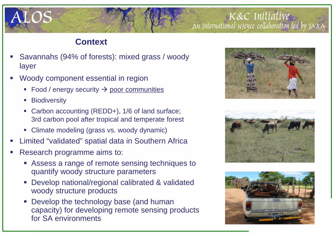
Context Savannahs (94% of forests): mixed grass / woody
layer Woody component essential in region
Food / energy security poor communities Biodiversity Carbon accounting (REDD+), 1/6 of land surface;
3rd carbon pool after tropical and temperate forest Climate modeling (grass vs. woody dynamic)
Limited “validated” spatial data in Southern Africa Research programme aims to: Assess a range of remote sensing techniques to
quantify woody structure parameters Develop national/regional calibrated & validated
woody structure products Develop the technology base (and human
capacity) for developing remote sensing products for SA environments
MODIS Vegetation Continuous FieldMODIS Vegetation Continuous Field
Tropical Africa’s above-ground biomass
Tropical Africa’s above-ground biomass
ICESat Global Tree Height Map
ICESat Global Tree Height Map
ALOS PalSAR 10 m Global forest map
ALOS PalSAR 10 m Global forest map
% tree cover, herbaceous, and bare, annual product,
500 m
Green economy
Nationally households use 4.5-6.7 million T / yr of wood for energy to a value of R3 billion. Savings on new electricity generation between USD14.6-77.4 million per yr
Policy on Woodlands
Medium Term Strategic Framework Outcome 10 led by DEA“Net deforestation to be maintained at no more than 5% woodlands by 2020”“Undertake provincial and national forest resource assessment programs”
Policy on Woodlands
National Forests Act (84 of 1998) caters for woodlands and recognizes them explicitly as renewable energy source. The Act makes provision for research, monitoring, dissemination of information and reporting. DAFF has legally to report every three years on the status of woodlands to the minister.

Arid / semi-arid: 10-50% woody cover, < 60 woody T/ha ABG
Mostly gradual changes: logging, encroachment Fine scale heterogeneity = remote sensing challenge Woody plant size & cover (3-6 m, 10-40%) Soil properties & water availability Disturbance factors: fire, herbivore, human
Woody plant: multi-stemmed clumps, high biomass in branches rather than in main stem
Savannahs & woodlands in southern Africa

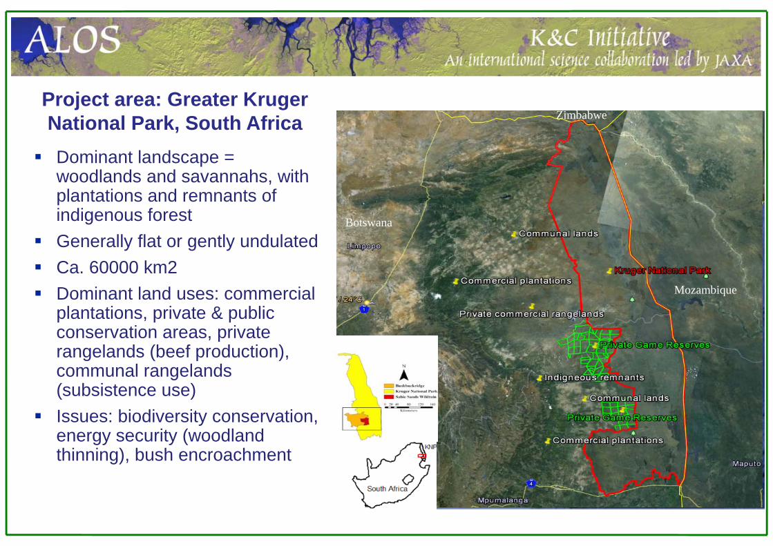
Dominant landscape = woodlands and savannahs, with plantations and remnants of indigenous forest
Generally flat or gently undulated Ca. 60000 km2 Dominant land uses: commercial
plantations, private & public conservation areas, private rangelands (beef production), communal rangelands (subsistence use)
Issues: biodiversity conservation, energy security (woodland thinning), bush encroachment
Mozambique
Botswana
ZimbabweProject area: Greater Kruger National Park, South Africa

Data currently available
Ground Woody cover (N= 37) and
biomass plots (N= 152) Airborne LiDAR 2008, 10 & 12 (Carnegie
Airborne Observatory) – end wet season
Satellite SAR: Radarsat-2 (C-band),
ALOS-1 PALSAR (L-band), TerraSAR-X (X-band)
High res SAR biomass / cover mapping
Medium res SAR biomass / cover mapping
Flux tower Phalaborwa
Flux tower Skukuza
General objective: assess and develop “affordable” methods to predict woody cover and biomass in southern African woodlands and savannahs using SAR imagery
Secondary objectives: Investigate the potential of combining multiple SAR frequencies (L-band
ALOS PalSAR, C-band Radarsat-2, X-band TerraSAR-X) Optical / SAR “fusion” Investigate full polarimetric ALOS PalSAR / RADARSAT-2 imagery and
polarimetric decompositions Change detection of woody cover for complete Kruger National Park using
ALOS PalSAR (2008-2010) and JERS-1 / Landsat (2000)
Project objectives and schedule
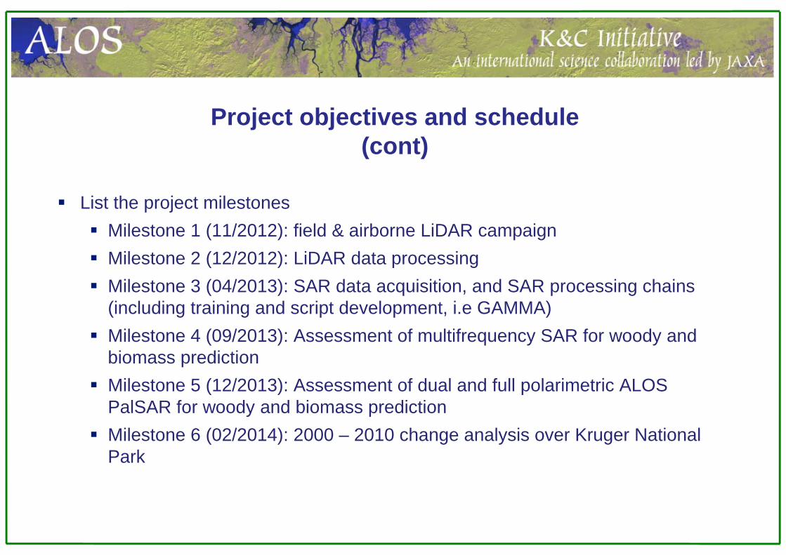
List the project milestones Milestone 1 (11/2012): field & airborne LiDAR campaign Milestone 2 (12/2012): LiDAR data processing Milestone 3 (04/2013): SAR data acquisition, and SAR processing chains
(including training and script development, i.e GAMMA) Milestone 4 (09/2013): Assessment of multifrequency SAR for woody and
biomass prediction Milestone 5 (12/2013): Assessment of dual and full polarimetric ALOS
PalSAR for woody and biomass prediction Milestone 6 (02/2014): 2000 – 2010 change analysis over Kruger National
Park
Project objectives and schedule (cont)
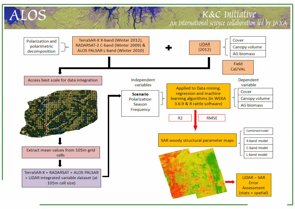
General methodology
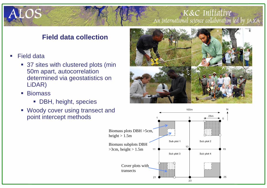
Field data collection
Field data 37 sites with clustered plots (min
50m apart, autocorrelation determined via geostatistics on LiDAR)
Biomass DBH, height, species
Woody cover using transect and point intercept methods
Biomass subplots DBH >3cm, height > 1.5m
Cover plots with transects
Biomass plots DBH >5cm, height > 1.5m

LiDAR-based structural variables
Woody cover: area vertically projected on a horizontal plane (%)
Canopy volume: approximated from integration of vertical profile of laser hits
Biomass: Linear model between field AGB and LiDAR woody cover and height metrics
Woody coverWoody cover
Height
CanopyIntegration of vertical profile = canopy volume
Hei
ght
Canopy volumeCanopy volume
Above ground biomassAbove ground biomass
Methods after Colgan et al, 2012, Biogeosci. Disc

LiDAR-based cal/cal: height and cover
Field metric
LiD
AR
met
ric
Height
Woody cover
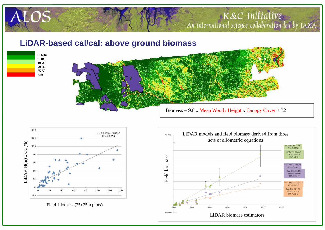
0 T/ha0-1010-2020-3535-50>50
LiD
AR
H(m
) x C
C(%
)
Field biomass (25x25m plots)
Biomass = 9.8 x Mean Woody Height x Canopy Cover + 32
LiDAR models and field biomass derived from three sets of allometric equations
LiDAR biomass estimators
Fiel
d bi
omas
s
LiDAR-based cal/cal: above ground biomass

SAR processing
Bush clearing
Riparian zones
Fire break
Fire scar
Settlements
Radarsat‐2 image , dry season
Geocoded (90m SRTM DEM) final resolution: 12.5m
Geocoded (90m SRTM DEM) final resolution: 5m
Geocoded (90m SRTM DEM) final resolution: 3m
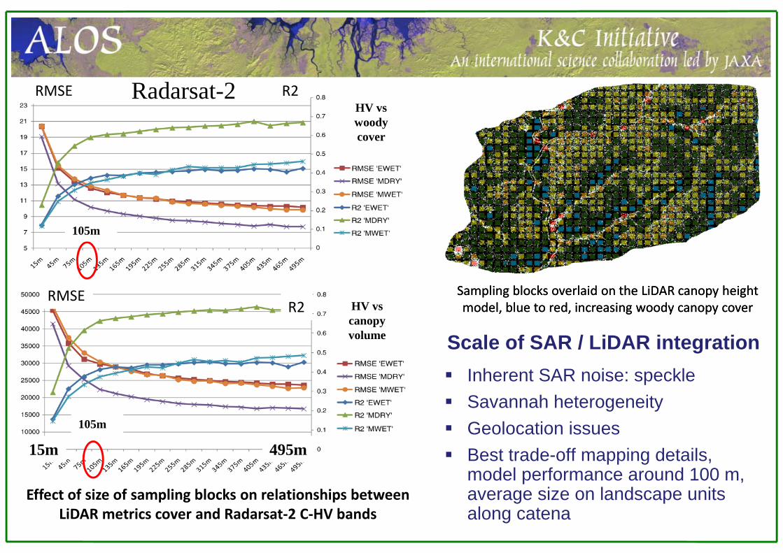
Sampling blocks overlaid on the LiDAR canopy height model, blue to red, increasing woody canopy coverSampling blocks overlaid on the LiDAR canopy height model, blue to red, increasing woody canopy coverR2
15m
RMSE
Effect of size of sampling blocks on relationships between LiDAR metrics cover and Radarsat‐2 C‐HV bands
495m
105m
RMSE R2
105m
Inherent SAR noise: speckle Savannah heterogeneity Geolocation issues Best trade-off mapping details,
model performance around 100 m, average size on landscape units along catena
HV vs woody cover
HV vs canopy volume Scale of SAR / LiDAR integration
Radarsat-2
125m 200m
50m25m
PALSAR

Season
Strong change of vegetation condition – water balance with season and phenology Middle Wet (Summer) – grass
green and woody leaf-on End of Wet (Autumn) – grass dry
and woody leaf-on Dry (Winter) – grass dry and woody
leaf-off Early Wet (Spring) – grass dry and
woody leaf-on Best is dry season, than middle
wet, and end of wet (early wet?) Low moisture effect, higher
penetration (high frequency) Similar pattern for L- and C-band
Mean R² between PALSAR HH backscatter intensity and LiDAR-based woody cover at four aggregation levels (DRY dry season; EWET end of wet season;
MWET middle of wet season)
DRY MWET EWET
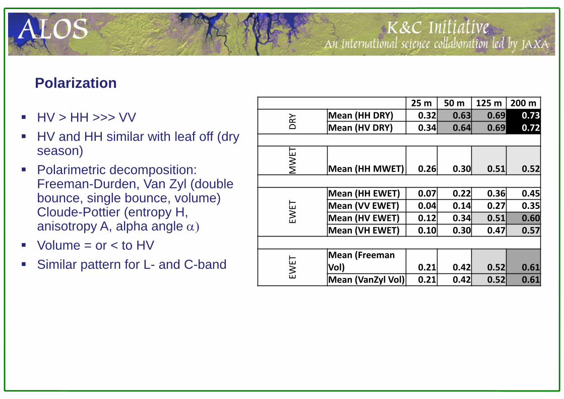
Polarization25 m 50 m 125 m 200 m
DRY Mean (HH DRY) 0.32 0.63 0.69 0.73
Mean (HV DRY) 0.34 0.64 0.69 0.72
MWET
Mean (HH MWET) 0.26 0.30 0.51 0.52
EWET
Mean (HH EWET) 0.07 0.22 0.36 0.45Mean (VV EWET) 0.04 0.14 0.27 0.35Mean (HV EWET) 0.12 0.34 0.51 0.60Mean (VH EWET) 0.10 0.30 0.47 0.57
EWET
Mean (Freeman Vol) 0.21 0.42 0.52 0.61Mean (VanZyl Vol) 0.21 0.42 0.52 0.61
HV > HH >>> VV HV and HH similar with leaf off (dry
season) Polarimetric decomposition:
Freeman-Durden, Van Zyl (double bounce, single bounce, volume) Cloude-Pottier (entropy H, anisotropy A, alpha angle
Volume = or < to HV Similar pattern for L- and C-band
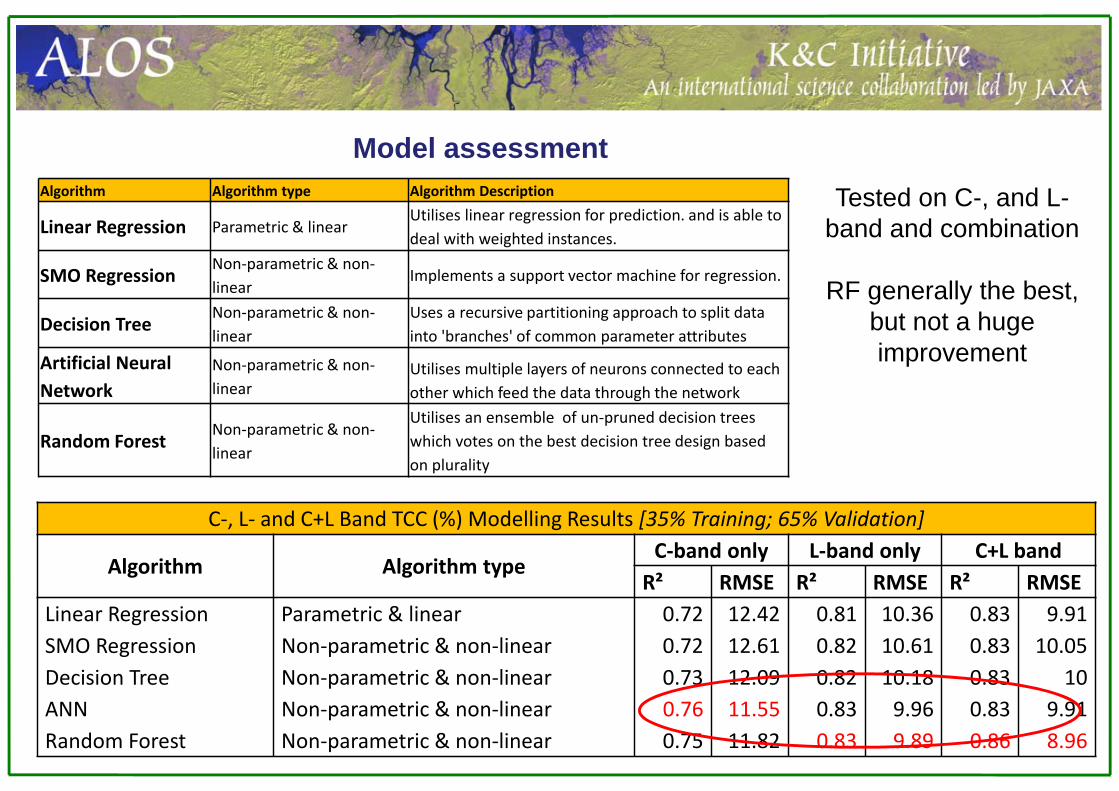
Model assessmentAlgorithm Algorithm type Algorithm Description
Linear Regression Parametric & linearUtilises linear regression for prediction. and is able to deal with weighted instances.
SMO RegressionNon‐parametric & non‐linear
Implements a support vector machine for regression.
Decision TreeNon‐parametric & non‐linear
Uses a recursive partitioning approach to split data into 'branches' of common parameter attributes
Artificial Neural Network
Non‐parametric & non‐linear
Utilises multiple layers of neurons connected to each other which feed the data through the network
Random Forest Non‐parametric & non‐linear
Utilises an ensemble of un‐pruned decision trees which votes on the best decision tree design based on plurality
C‐, L‐ and C+L Band TCC (%) Modelling Results [35% Training; 65% Validation]
Algorithm Algorithm typeC‐band only L‐band only C+L band
R² RMSE R² RMSE R² RMSELinear Regression Parametric & linear 0.72 12.42 0.81 10.36 0.83 9.91SMO Regression Non‐parametric & non‐linear 0.72 12.61 0.82 10.61 0.83 10.05Decision Tree Non‐parametric & non‐linear 0.73 12.09 0.82 10.18 0.83 10ANN Non‐parametric & non‐linear 0.76 11.55 0.83 9.96 0.83 9.91Random Forest Non‐parametric & non‐linear 0.75 11.82 0.83 9.89 0.86 8.96
Tested on C-, and L-band and combination
RF generally the best, but not a huge improvement
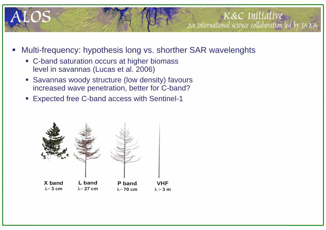
Multi-frequency: hypothesis long vs. shorther SAR wavelenghts C-band saturation occurs at higher biomass
level in savannas (Lucas et al. 2006) Savannas woody structure (low density) favours
increased wave penetration, better for C-band? Expected free C-band access with Sentinel-1
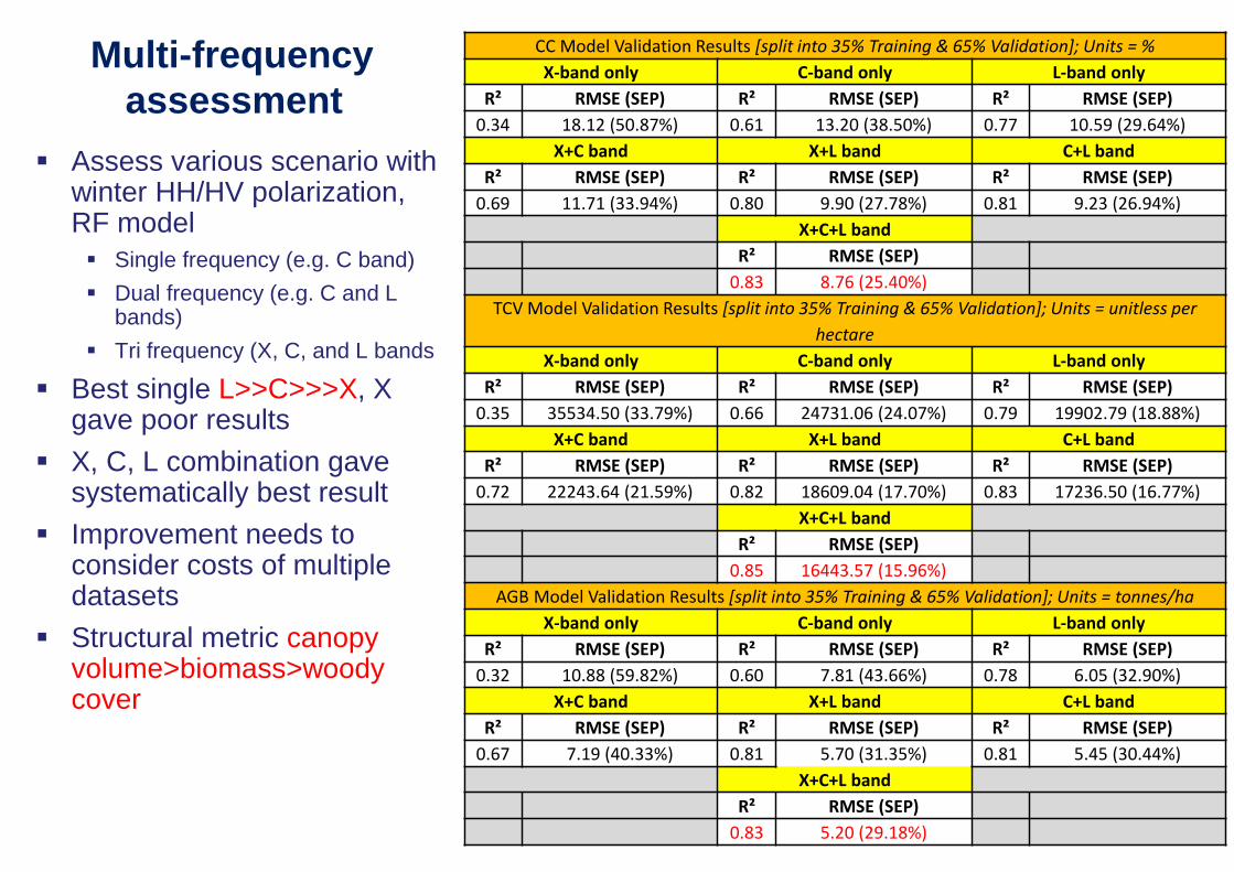
Multi-frequency assessment
CC Model Validation Results [split into 35% Training & 65% Validation]; Units = %X‐band only C‐band only L‐band only
R² RMSE (SEP) R² RMSE (SEP) R² RMSE (SEP)0.34 18.12 (50.87%) 0.61 13.20 (38.50%) 0.77 10.59 (29.64%)
X+C band X+L band C+L bandR² RMSE (SEP) R² RMSE (SEP) R² RMSE (SEP)0.69 11.71 (33.94%) 0.80 9.90 (27.78%) 0.81 9.23 (26.94%)
X+C+L bandR² RMSE (SEP)0.83 8.76 (25.40%)
TCV Model Validation Results [split into 35% Training & 65% Validation]; Units = unitless per hectare
X‐band only C‐band only L‐band onlyR² RMSE (SEP) R² RMSE (SEP) R² RMSE (SEP)0.35 35534.50 (33.79%) 0.66 24731.06 (24.07%) 0.79 19902.79 (18.88%)
X+C band X+L band C+L bandR² RMSE (SEP) R² RMSE (SEP) R² RMSE (SEP)0.72 22243.64 (21.59%) 0.82 18609.04 (17.70%) 0.83 17236.50 (16.77%)
X+C+L bandR² RMSE (SEP)0.85 16443.57 (15.96%)
AGB Model Validation Results [split into 35% Training & 65% Validation]; Units = tonnes/haX‐band only C‐band only L‐band only
R² RMSE (SEP) R² RMSE (SEP) R² RMSE (SEP)0.32 10.88 (59.82%) 0.60 7.81 (43.66%) 0.78 6.05 (32.90%)
X+C band X+L band C+L bandR² RMSE (SEP) R² RMSE (SEP) R² RMSE (SEP)0.67 7.19 (40.33%) 0.81 5.70 (31.35%) 0.81 5.45 (30.44%)
X+C+L bandR² RMSE (SEP)0.83 5.20 (29.18%)
Assess various scenario with winter HH/HV polarization, RF model Single frequency (e.g. C band) Dual frequency (e.g. C and L
bands) Tri frequency (X, C, and L bands
Best single L>>C>>>X, X gave poor results
X, C, L combination gave systematically best result
Improvement needs to consider costs of multiple datasets
Structural metric canopy volume>biomass>woody cover

Va
X TCC C TCC L TCC
X+C TCC X+L TCC C+L TCC
X+C+L TCC
Validation of woody cover model
From short to longest wavelength and addition of
bands tend to decrease over estimation and
underestimation at low and high density

Va
Validation of canopy volume model
X TCV C TCV L TCV
X+C TCV X+L TCV C+L TCV
X+C+L TCV

Dense sector
Scattered sector
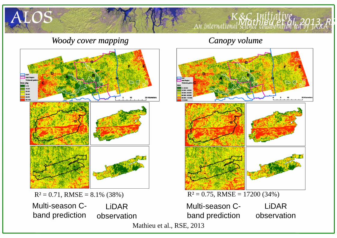
R² = 0.71, RMSE = 8.1% (38%)
Woody cover mappingWoody cover mapping
Mathieu et al, 2013, RSE
Canopy volumeCanopy volume
R² = 0.75, RMSE = 17200 (34%)
Multi-season C-band prediction
LiDAR observation
Multi-season C-band prediction
LiDAR observation
Mathieu et al., RSE, 2013
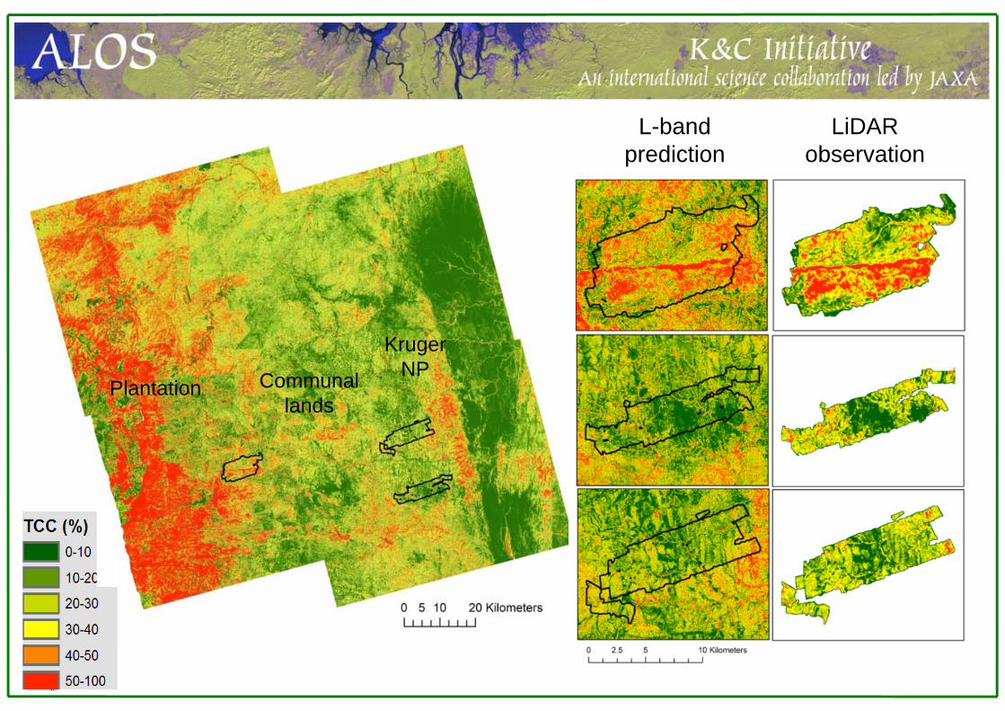
L-band prediction
LiDAR observation
Kruger NPCommunal
landsPlantation

Provincial up scaling
Total canopy cover maps from ALOS PalSAR L-band in the South African Loweld.
Need more extended cal/val
Maps are produced using random forest models and dual pol (HH/HV), 14 scene mosaic.
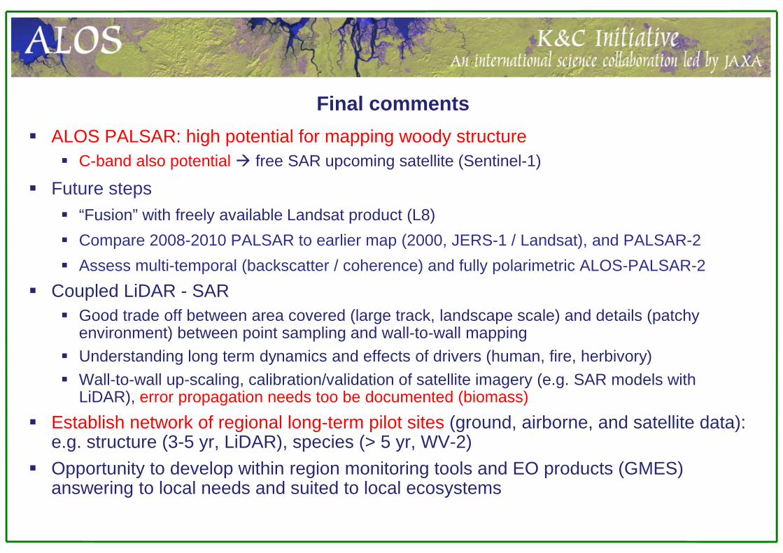
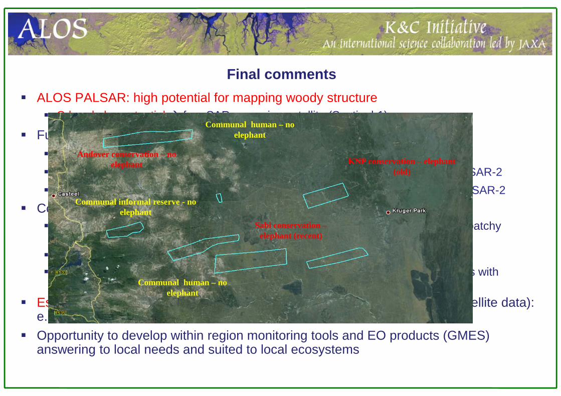
Final comments ALOS PALSAR: high potential for mapping woody structure
C-band also potential free SAR upcoming satellite (Sentinel-1)
Future steps “Fusion” with freely available Landsat product (L8) Compare 2008-2010 PALSAR to earlier map (2000, JERS-1 / Landsat), and PALSAR-2 Assess multi-temporal (backscatter / coherence) and fully polarimetric ALOS-PALSAR-2
Coupled LiDAR - SAR Good trade off between area covered (large track, landscape scale) and details (patchy
environment) between point sampling and wall-to-wall mapping Understanding long term dynamics and effects of drivers (human, fire, herbivory) Wall-to-wall up-scaling, calibration/validation of satellite imagery (e.g. SAR models with
LiDAR), error propagation needs too be documented (biomass) Establish network of regional long-term pilot sites (ground, airborne, and satellite data):
e.g. structure (3-5 yr, LiDAR), species (> 5 yr, WV-2) Opportunity to develop within region monitoring tools and EO products (GMES)
answering to local needs and suited to local ecosystems
KNP conservation – elephant (old)
Sabi conservation –elephant (recent)
Andover conservation – no elephant
Communal human – no elephant
Communal informal reserve - no elephant
Communal human – no elephant
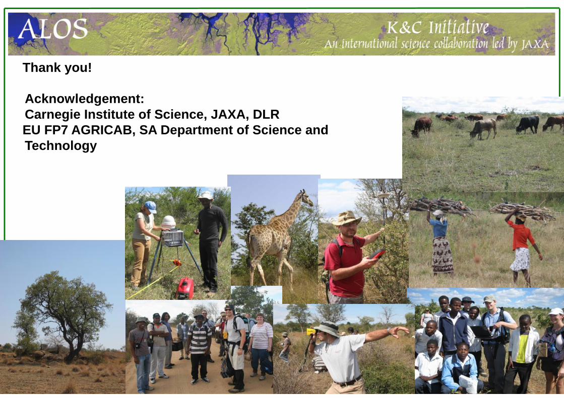
Thank you!
Acknowledgement: Carnegie Institute of Science, JAXA, DLREU FP7 AGRICAB, SA Department of Science and Technology