assessing whether soil moisture content (smc) can be
TRANSCRIPT

Assessing whether Soil Moisture Content (SMC) can be estimated for wetlands in the grassland biome of South Africa using freely
available space-borne sensors
By
Ridhwannah Gangat
For a full Master’s thesis:
A thesis submitted in partial fulfilment of the requirements for the degree of Master
Scientiae in the Faculty of Science, University of Witwatersrand
Supervisor: Dr. Heidi Van Deventer
Co-supervisor: Dr. Laven Naidoo
Co-supervisor: Dr. Elhadi Adam
May 2019
ABSTRACT
Soil moisture content (SMC) takes on an important role in the hydrological
functioning of wetlands. Temperature increases associated with climate change is
expected to impact the hydrological regime of wetlands. Therefore, regional
monitoring of SMC is essential for improved understanding of potential changes to
the hydrological regime of wetlands while supporting decision making and
interventions. Conventional methods of measuring SMC are costly and have a
limited view of processes occurring at regional to global scales. In contrast, remote
sensing can potentially offer a regular, regional overview of the hydrological function
of wetlands and is therefore more cost-affordable compared to conventional
methods. In the past, estimations of SMC with remote sensing lacked a sufficient
spatial resolution for palustrine inland wetland ecosystem types, particularly in semi-
arid countries. However, the use of recently launched and freely available high
spatial resolution sensors, such as the Sentinel series, may overcome these
limitations. In this study, the use of European Space Agency’s Sentinel-1A and 1B
(S1A, S1B; Synthetic Aperture Radar) and Sentinel-2A and 2B (S2A, S2B; optical)
sensors were evaluated for their ability to predict SMC for wetlands and drylands in
the grassland biome of South Africa. The percentage Volumetric Water Content
(%VWC) for 200 points was measured in the Colbyn Nature Valley which is
dominated by a palustrine wetland. The %VWC in the wetlands and terrestrial area
of the study area were measured using a hand-held SMT-100 soil moisture and
temperature meter at a 5 cm soil depth during March and May 2018 (the peak of the
hydroperiod) and regressed against the Synthetic Aperture Radar (SAR) and optical
data using a parametric and non-parametric models. The results showed that
Sentinel images can predict the percentage SMC, with both the S1B and S2B
images achieving the highest coefficient of determinations (R² > 0.8; R² > 0.9) and
relatively low Root Mean Square Errors (RMSE = 10 %; 12 %) respectively.
Predicted maps showed significantly lower ranges of SMC below 50 % (p ≤ 0.05) in
the terrestrial area compared to the higher ranges of SMC (≥ 50 %) in wetlands for
both sensors. Although the SAR C-band is limited to the upper 5 cm of the soil
depth, it shows potential to measure ranges of SMC for palustrine wetlands and
terrestrial areas in the grassland biome of South Africa which will be beneficial for
wetland inventorying.
Key words: Sentinel-1; Sentinel-2; soil moisture content; volumetric water content; palustrine
wetlands; hydroperiod; Random Forest regression; machine learning regression

DECLARATION
I ____Ridhwannah Gangat_______ (Student number: __1814325__) am a student registered for _ SRA00 – Masters of science (Dissertation)_____ in the year ____2019______. I hereby declare the following:
I am aware that plagiarism (the use of someone else’s work without their permission and/or without acknowledging the original source) is wrong.
I confirm that ALL the work submitted for assessment for the above course is my own unaided work except where I have explicitly indicated otherwise.
I have followed the required conventions in referencing the thoughts and ideas of others.
I understand that the University of the Witwatersrand may take disciplinary action against me if there is a belief that this is not my own unaided work or that I have failed to acknowledge the source of the ideas or words in my writing.
Signature: _____ ________ Date: ___19 March 2019_________
ACKNOWLEDGEMENTS
Firstly, I want to thank the Almighty for giving me the strength and courage to
complete this journey.
To my supervisor, Dr. Heidi van Deventer, how can I ever possibly thank you for the
unconditional support you have given me ever since I met you and without you this
project wouldn’t have been possible. You introduced me to remote sensing and
guided me through scientific research. Through you, I learned the dedication of a
researcher, persistence and earnestness. For all my life, I will never forget what you
have done for me!
To my co-supervisor, Dr. Laven Naidoo, your expertise in remote sensing, visionary
thoughts and working style has made a deep impression on me. I want to thank you
for always being available when I needed advice, your suggestions and valuable
feedback improved this project greatly. You acted as a pillar of strength and always
encouraged me to do my best.
Dr. Elhadi Adam, for contributing to the development of this work.
To my mom, dad and siblings, for all the support and encouraging words throughout
the duration of this research.
In particular, thanks to Heidi Van Deventer, Laven Naidoo, Razeen Gangat,
Mohamed Gangat, Taskeen Gangat, Zahra Varachia, Salman Mia, Yonwaba Atyosi
and Jason Le Roux who helped me in acquiring in situ measurements, especially in
the worst conditions. A special thanks to Tamsyn Sherwill for including me in all of
Colbyn Nature Valley Reserve projects and conservation initiatives.

Table of Contents
List of Tables................................................................................................................i
List of Figures...............................................................................................................ii
List of Equations..........................................................................................................iv
Chapter 1 : GENERAL INTRODUCTION ................................................................... 1
1.1. The Importance of estimating and monitoring soil moisture content of wetlands ........... 2
1.2. Regional monitoring of the variation and changes in the soil moisture content of
wetlands ............................................................................................................................................. 5
1.3. Motivation................................................................................................................................... 9
1.4. Study area ............................................................................................................................... 10
1.5 Aim and objectives .................................................................................................................. 11
1.6. Thesis outline .......................................................................................................................... 12
Chapter 2 : LITERATURE REVIEW ......................................................................... 13
2.1 Wetlands ................................................................................................................................... 14
2.1.1 Definitions and concepts ................................................................................................. 14
2.1.2 Wetlands under pressure ................................................................................................ 18
2.1.3 Inventorying and monitoring of palustrine wetlands in South Africa ......................... 19
2.2 Soil moisture content ............................................................................................................... 21
2.2.1 The role of soil moisture content in wetlands ............................................................... 21
2.2.2 In situ soil moisture measurements ............................................................................... 22
2.3 Remote sensing approaches for estimating near surface soil moisture content ........... 26
Chapter 3 : MATERIALS AND METHODS ............................................................... 36
3.1 Study area................................................................................................................................. 37
3.1.1 Description of study area ................................................................................................ 37
3.1.2 Climate ............................................................................................................................... 39
3.1.3 Vegetation ......................................................................................................................... 39
3.2 Data collection .......................................................................................................................... 40
3.2.1 Image acquisition and pre-processing .......................................................................... 40
3.2.2 In situ soil moisture measurements ............................................................................... 42
3.3 Data analysis ............................................................................................................................ 44
Chapter 4 : RESULTS .............................................................................................. 49
4.1 Descriptive statistics analysis and normality testing for in situ volumetric water content
measurements ................................................................................................................................ 50
4.2 Ability of Sentinel-1 and Sentinel-2 to estimate soil moisture content ............................. 52

4.3 Differences in soil moisture content between wetland and terrestrial ecosystem types
.......................................................................................................................................................... 56
Chapter 5 : DISCUSSION ........................................................................................ 62
Chapter 6 : CONSCLUSION .................................................................................... 69
Chapter 7 : REFERENCES ...................................................................................... 71
i
LIST OF TABLES
Table 1: Types of definitions used for wetland inventories (Source: Adapted from Tiner et al., 2015:7)
.............................................................................................................................................................. 14
Table 2: Summary of the advantages and disadvantages of each different remote sensing
technologies method to in retrieving soil moisture content (Adapted from Barret et al., 2012:87). .. 27
Table 3: Acquisition dates and times of the Sentinel 1A/1B and Sentinel 2A/2B images as well as the
dates of ground measurements. ........................................................................................................... 41
Table 4: Spectral bands and associated wavelength ranges of the optical Sentinel 2A and 2B images
(adapted from ESA Sentinel online, 2019). ........................................................................................... 42
Table 5: Descriptive statistical analysis illustrating the variability of soil moisture across the study site
during the March and May 2018 sampling campaigns ......................................................................... 50
Table 6: Comparison of the different modelling approaches and validation models, using coefficient
of determination (R²) and Root Mean Square Error (RMSE) between the percentage Volumetric
Water Content (%VWC) and predicted percentage of Soil Moisture Content (%SMC), across the four
Sentinel sensors evaluated, using simple linear regression, support vector machine and random
forest modelling algorithms. S1A = Sentinel 1A; S1B = Sentinel 1B; S2A = Sentinel 2A; S2B = Sentinel
2B; VV = vertical-receive, vertical-transmit; VH = vertical receive, horizontal-transmit;
VRE = Vegetation Red Edge; SWIR = Short Wave Infrared; SLR = simple linear regression; SVM =
support vector machine; RF = random forest. ...................................................................................... 54
Table 7: Differences between the wetland and terrestrial areas for in situ percentage Volumetric
Water Content (%VWC) and Soil Moisture Content (%SMC) resulting from the Sentinel 1B and 2B
predictions. ........................................................................................................................................... 56
Table 8: Descriptive statistics for in situ observed percentage of Volumetric Water Content (%VWC)
and predicted percentage of Soil Moisture Content (%SMC) at the time of Sentinel sensors overpass
on the 28 March 2018 for Sentinel-1B and on 2 May 2018 for Sentinel-2B. ....................................... 58

ii
LIST OF FIGURES
Figure 1: Six -tiered hierarchical structure based on the characteristics of the South African
Classification System for Wetlands and other Aquatic Ecosystems (Ollis et al., 2013:6). Soil moisture
saturation regimes are attributed at Level 5. ....................................................................................... 16
Figure 2: A diagram of a wetland representing the difference between the saturation and inundation
zones (Source: Ollis et al., 2013:41) ...................................................................................................... 17
Figure 3:The shorter microwave wavelength (X-band, 3cm) interacts mostly with the top of the
canopy cover, while longer wavelengths (L-band, 24 cm) penetrate further into the canopy and
reflect from the soil surface (adapted from Barrett and Petropoulos, 2012: 91) ................................ 31
Figure 4: Three types of scattering (transmit and receive signals) depending on target (Source:
adapted and modified from: Bai et al. (2017a:186). ............................................................................ 33
Figure 5: The location of the study area, the Colbyn Valley Nature Reserve (CVNR), is located within
the Gauteng Province of South Africa (a). The CVNR hosts a channelled valley-bottom wetland (b)
through which the Hartebeesspruit (River) runs. The location of sample plots is displayed in the
wetland and terrestrial areas. ............................................................................................................... 38
Figure 6: Mean monthly precipitation for 2017 and 2018 (especially during sampling periods)
according to the Station 30687 situated in Pretoria, South Africa (ARC-ISCW, 2018). ........................ 39
Figure 7: Vegetation found in the wetland area varying from Typha capensis to Imperata cylindrica
during end of peak growing season (left and right, respectively). ....................................................... 40
Figure 8: Diagram illustrating the planning of sampling according to the Sentinel 1 and 2 image
pixels. The smalls (green) squares represent the in situ sampling measurements that were
specifically located with both Sentinel 1 and Sentinel 2 pixels (blue outline) to ensure values could be
extracted for both sensor’s pixels. ........................................................................................................ 43
Figure 9: Flowchart illustrating the different stages of the overall procedure and methodology to
generate the final outcome of a predicted percentage Soil Moisture Content (%SMC) maps. ........... 47
Figure 10: Graphs showing the distribution of the percentage Volumetric Water Content (%VWC) for
(a) 28 March 2018 and (b) 2 May 2018. The results from the Shapiro-Wilk test indicates the in situ
percentage Volumetric Water Content in not normally distributed (p < 0.05). ................................... 51

iii
Figure 11: Percentage Volumetric Water Content and predicted percentage of Soil Moisture Content
levels between drylands and wetlands for (a) 28 March 2018 and (b) 2 May 2018 ........................... 56
Figure 12: Predicted percentage Soil Moisture Content (%SMC) map derived from Sentinel-1B
showing the variation in soil moisture on 28 March 2018 sampling campaign. .................................. 59
Figure 13: Predicted percentage Soil Moisture Content (%SMC) map derived from Sentinel-2B
showing the variation in soil moisture for 2 May 2018 sampling campaign. ....................................... 60
Figure 14: Standard error regression graphs displaying how well Sentinel 1B (a) and Sentinel 2B (b)
captured the variability of the soil moisture content across the study area. ...................................... 61
Figure 15: Precipitation readings for the duration of the sampling period. Graph (a) shows a rainfall
period shortly before the acquisition for S1B on the 28 March 2018 (indicated by red arrow) and
graph (b) the S2B acquisition on 2 May2018 (indicated by red arrow). Scale ranges are different to
account for differences in the maximum precipitation of the two sample dates. ............................... 65

iv
LIST OF EQUATIONS
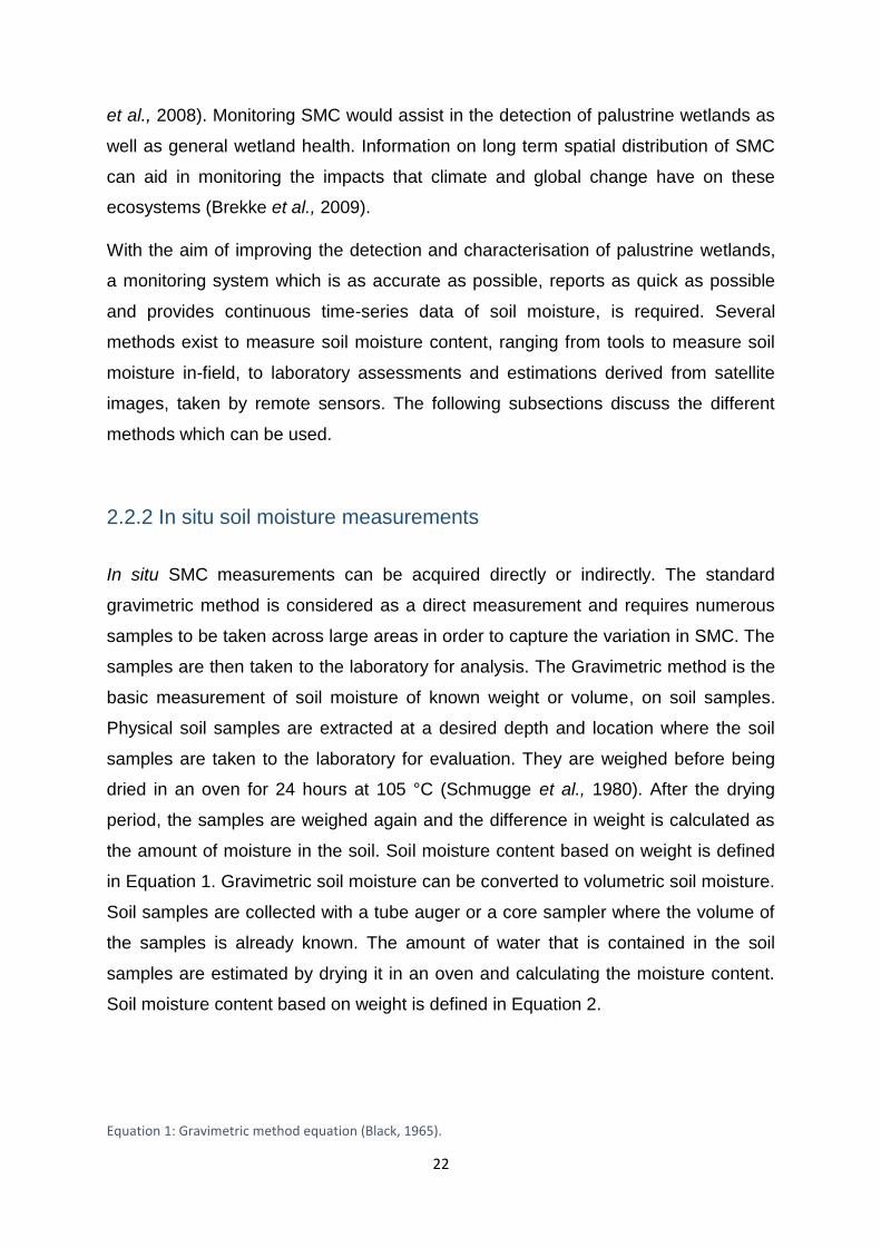
Equation 1: Gravimetric method equation (Black, 1965). .................................................................... 22
Equation 2: Volumetric Water Content equation (Black, 1965). .......................................................... 23
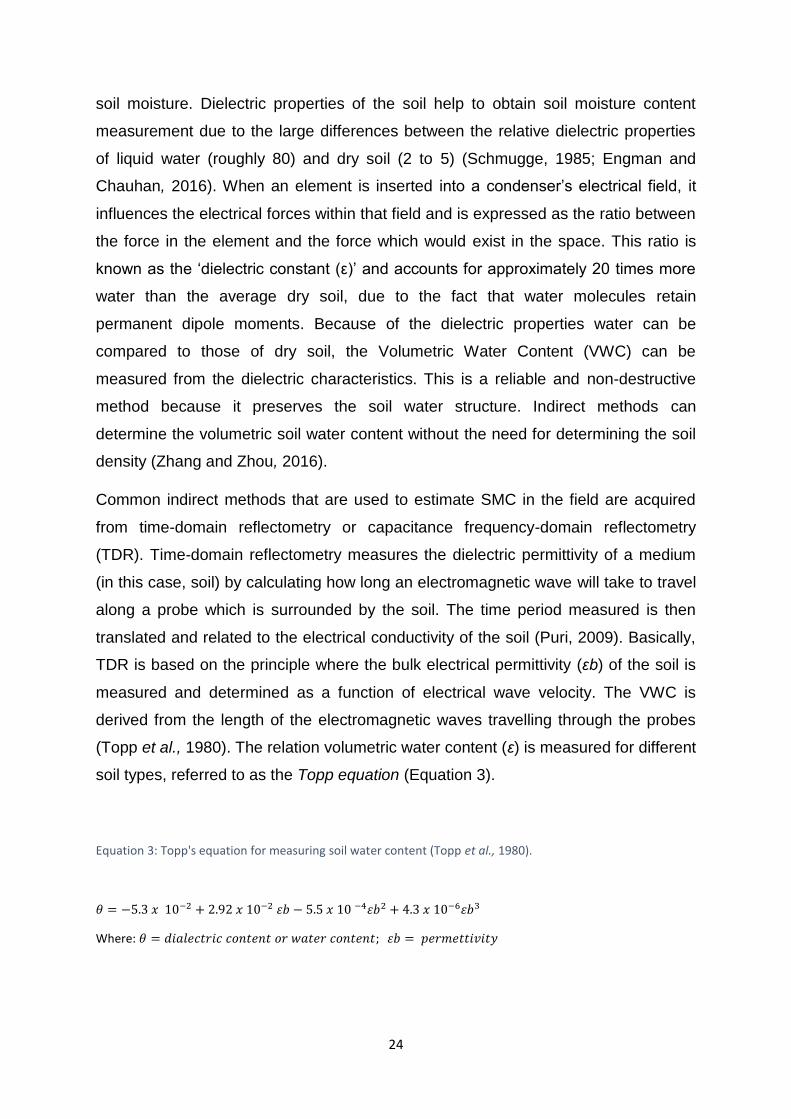
Equation 3: Topp's equation for measuring soil water content (Topp et al., 1980). ............................ 24

1
Chapter 1 : GENERAL INTRODUCTION
2
1.1. The Importance of estimating and monitoring soil moisture
content of wetlands
Soil moisture is an important attribute in wetland extent and dynamics. The National
Wetland Maps showed that wetlands occupy only a small portion of South Africa’s
surface area (Van Deventer et al., 2018b). Despite their small extent, they offer
various ecological and economical functions which include improving water quality,
flood and drought regulation, groundwater recharge, habitation for animals and
plants, agricultural production and assist in managing limited water resources in the
country and support commercial activities (McLaughlin et al., 2013). Different
definitions of the term ‘wetlands’ have been used across the world (e.g., Burton and
Tiner, 2009). Wetlands are areas of soil saturated or inundated with water within 50
cm from the soil surface, which occurs during water periods or long enough
throughout the growing season to become anoxic (Burton and Tiner, 2009; Ollis et
al., 2013:1).
South Africa has a variable climate resulting in the formation of a variety of wetland
types. The Classification System for Wetlands and other Aquatic Ecosystems (Ollis
et al., 2013) in South Africa distinguished three types of wetlands such as marine,
estuarine and inland systems. Unlike marine and estuarine systems, inland systems
are not connected to large bodies of water like the sea (Ollis et al., 2013). Inland
aquatic ecosystems are systems that are found in different locations and natural
settings, and hold a wide range of unique properties and functions.
Wetlands continue to decline on a global scale, in extent and quality, to such severe
standards, placing these ecosystems under pressure as well as the services they
provide such as supplying water or providing habitation for wildlife (Gardner et al.,
2015). Wetlands have been and are subjected to various stress induced
modifications like polluted runoff, hydrological modifications, eutrophication and,
more recently a major concern is the impact from global climate change (Levin et al.,
2001). Global changes are a major contribution to the degradation and loss of
wetlands, these include: a higher demand for water supply due to an increasing
population, urbanisation, infrastructure and development, agricultural activities such
as overgrazing and increased water abstraction for irrigation purposes (Russi et al.,
3
2013). In addition to global changes, climate change poses as a huge threat to the
ecological condition of wetlands due to increasing temperatures and
evapotranspiration. Over the last few years, an unequivocal increase in temperature
of 1.5 °C have been observed while, it had been predicted that by 2050 the
temperature is likely to exceed 2 °C (IPCC, 2014). In addition, a general decrease in
precipitation in lower latitudes is expected to occur (Day et al., 2005). Examples of
impacts that occur from climate change include, alterations in the base flow, changes
in hydrology (for example changes in wet and dry periods due increasing
temperatures), increased weather events such as floods and droughts and a
decrease in water quantity, to name a few (STRP, 2002).
To overcome these challenges, regular monitoring of the spatial extent of inland
wetlands is required to identify how much and where losses are occurring. However,
inland wetlands are highly variable in spatial extent because the inundated and
saturated areas change periodically, and often seasonally (Hess et al., 2015; Li et
al., 2015). While inundation have been monitored well across the globe for larger
wetlands (e.g. Pekel et al., 2016), monitoring of palustrine (vegetated) wetlands are
deficient. Monitoring of Soil Moisture Content (SMC) can serve as a possible
indicator of wetland functionality in palustrine wetlands and could be valuable for
wetland inventorying too. SMC acts as an important component in the hydrological
processes in wetlands leading to the understanding of land-surface interactions and
has a predominant influence on an ecosystem’s response to the physical
environment (Wei, 1995; Martinez et al., 2014). Because of the spatial variability that
characterise the earth surface in terms of soil (e.g. slope and texture), as well as
other processes that influence the water fluxes of near surface soil moisture (e.g.
precipitation and evapotranspiration), soil moisture is variable in both space and
time. Near surface soil moisture is considered to correspond to the upper layer
(~5 cm) in the top soil (Bousbih et al., 2018).
Assessing soil moisture levels is particularly useful for determining the seasonal
patterns of water levels in a wetland, otherwise known as ‘hydroperiod’ or
‘hydrological regime’ (Erwin, 2008). These seasonal variations describe the
hydrological characteristics of a wetland, for example, whether it is inundated and for
how long (permanent, seasonal, intermittent); and is used as a criterion to determine
wetland types (Mitsch and Gosselink, 2007). A number of factors influence a

4
wetland’s hydroperiod, such as overgrazing from agricultural use or climate change.
Therefore, monitoring the hydrodynamics of a wetland provides an understanding of
a wetland’s response to the changes in their hydrology (Dixon, 2002; Voldseth et al.,
2007). More so, having insight to the hydrodynamics of a wetland is useful to
quantify the extent of a wetland and therefore a valuable asset to wetland
inventorying, especially in semi-arid countries (Conway and Dixon, 2000).
South Africa is a semi-arid country and experiences a mean annual rainfall (MAR) of
497 mm which falls below the global MAR of 860 mm (Bailey and Pitman, 2016). In
semi-arid regions, the amount of rainfall varies significantly within and between
seasons; as such, surface water availability can easily fluctuate (Klemas et al.,
2015). The scarcity of rainfall is compounded by the highly variable and uneven
distribution of rainfall in South Africa, where the western regions experiences less
run-off as compared to the eastern regions that receive a higher rainfall run-off
(Lumsden et al., 2009). The flow regime in wetlands is linked to rainfall events which
impacts the spatial and temporal distribution of soil moisture in inland aquatic
wetlands (Whitfield and Matlala, 2011). These effects are noticeable in the changes
of the hydrological period which may lead to the onset of increased
evapotranspiration and a reduction in the availability of soil moisture (Bullock and
Acreman, 2003; Dallas and Rivers-Moore, 2014; Brocca et al., 2017). This in turn
could accelerate the transformation and degradation of natural intact wetland
ecosystems and their associated ecosystem services. Due to the limited coverage of
wetlands in South Africa, their loss and degradation will result in severe
consequences as compared to a country with a larger extent of wetlands, especially
taking into consideration that South Africa is a semi-arid country (Kotze et al., 1996).
To compound monitoring efforts, in 2011, the South African National Biodiversity
Assessment reported that inland wetlands are poorly mapped, highly threatened and
poorly protected (Nel and Driver, 2012). Therefore, frequent monitoring, under global
and climate change conditions, is required to inform the status of the hydroperiod
and cycle in a non-destructive manner. There is a need for automated inventorying
of wetlands, particularly, palustrine wetlands which are poorly represented in the
National Wetland Map (NWM). Monitoring changes to SMC across the hydrological
cycle, at a regional scale, is important not only for addressing this shortcoming of the

5
NWM, but also future conservation strategies, decision making and intervention
bringing in great economic and societal benefits in South Africa.
1.2. Regional monitoring of the variation and changes in the soil
moisture content of wetlands
In recent decades, various methods have been developed to measure SMC at
different scales (Bittelli, 2011). There are several ways of measuring SMC. Firstly,
traditional in situ soil moisture measurements provide reliable point-scale data.
However, soil moisture is highly variable both spatially and temporally, therefore
direct measurements are not able to represent the spatial distribution of soil moisture
and is rendered inadequate to carry out regional to global scale monitoring (Engman,
1991; Wood et al., 1992). Three other disadvantages of direct measurements of
SMC are that it is labour intensive, time consuming and costly (Santi et al., 2013).
Obtaining accurate soil moisture in situ measurements in wetlands is also difficult
due to their dynamic hydrological characteristics, extensive areas which are difficult
to access and remote locations. In the past, surface hydrology models have been
developed to address the shortcomings of estimating SMC at a regional scale (Crow
and Yilmaz, 2014; Tebbs et al., 2016). The spatial scale of these applied models,
however, remains too fine scale (~10 km - ~100 km) for accurate soil surface
measurements of wetlands (Bloschl and Sivapalan, 1995; McDonnell et al., 2007;
Riley, 2014). Higher spatial resolution modelling is needed to produce more accurate
predictions in the terrestrial environment (Wood et al., 2011), particularly inland
wetlands of semi-arid to arid environments. Also, the large range of temporal scales
in hydrological modelling is limited because of a lack of up-to-date datasets for
modelling purposes, for example a time series of saturation or inundation levels and
water level discharge rates (Gentine et al., 2012).
Remote sensing technologies, both Synthetic Aperture Radar (SAR) and optical,
provides alternative tools for monitoring SMC of inland wetlands and to overcome
the limitations of small scale in situ measurements and coarse spatial resolution of
modelling SMC. International research has shown that space-borne sensors are able
to estimate SMC in the top layer (5 cm to 10 cm) of the soil surface and are capable
of producing regional estimates, with frequent temporal overpasses, and at a spatial
6
resolution ranging tens of kilometres (Wang and Qu, 2009). The capability of these
sensors remains to be assessed for South Africa’s palustrine wetlands.
Retrieving near surface soil moisture using various active and passive microwave
remote sensing techniques with good spatio-temporal resolution have been
conducted over primarily temperate and Mediterranean climates (Ulaby et al., 1982;
Su et al., 1997; Kerr et al., 2001; Njoku et al., 2002; Njoku et al., 2003; Moran et al.,
2004; Wigneron et al. 2007; Baghdadi et al., 2008; Parajka et al., 2009; Sinclair and
Pegram, 2010; Jackson et al., 2016). To date, these studies have used both C and
L-band sensors in their investigations, done for a wide variety of applications.
Different applications require different spatial and temporal resolutions (Al-Yaari,
2017). For instance, L-band passive remote sensing products are suitable for
acquiring SMC information at a global scale, ranging from tens of kilometres, such as
the Soil Moisture and Ocean Salinity (SMOS) at 35 km spatial resolution and the Soil
Moisture Active Passive (SMAP) satellite at 3 km spatial resolution with a temporal
resolutions of two to three days for both satellites (Klinke et al., 2018). However, the
low spatial resolution of L-band products does not account for the high spatial and
temporal variation of SMC which is unsuitable for monitoring of small spatial extent
ecosystems such as palustrine wetlands. More recently, active remote sensing C-
band SAR satellites have been employed in research studies due to its advantage to
provide near surface SMC datasets at medium to high spatial resolution (from 10 m
to 100 m) making it more suitable for detecting changes in wetlands, at a regional
scale, such as the European Remote Sensing Satellite 1/2 (ERS-1/2), Environmental
Satellite (ENVISAT) or RADARSAT-1/2 (Baghdad et al., 2008; Doubkova et al.,
2009; Pathe et al., 2009; Mladenova et al., 2010; Widhalm et al., 2015).
Two main features of microwave radiation are frequency and polarization. The depth
to which a microwave signal can penetrate depends on the frequency (f) and
wavelength of the satellite. Sensors with low frequency and longer wavelengths have
the ability to penetrate deeper into the soil surface such as the L-band (f = 1-2 GHz,
penetration depth = ~ 30 cm) as compared to higher frequency C-band (f = 4-8 GHz,
penetration depth = ~ 5 cm), and X-band (f = 8-12 GHz, penetration depth = ~3 cm)
sensors (Wagner et al., 2006). Ideally L-band sensors would therefore be more
suitable for monitoring wetlands, because of the ability to penetrate deeper in to the
soil surface near the estimated depth of saturation for wetlands (50 cm), however

7
owing to their coarse spatial resolution or low temporal resolution (e.g. ALOS sensor
has a revisit time of 46 days), users are limited to sensors at 5 cm depth for features
with smaller extents. In addition, estimating SMC becomes a challenge for high
frequency remote sensing products when the study area is also densely vegetated
and when there is high variability in the topography (e.g., surface roughness) (Ulaby
et al., 1979; Said et al., 2012). Several studies made use of C-band data to retrieve
SMC, however, the majority of these studies focused on the estimation of SMC in
terrestrial ecosystems, usually where the cover was bare soil or very little to sparsely
vegetated areas with correlation of determination (R) of > 0.5 and root square mean
error (RMSE) of ≤ 40 % (Moran et al., 2004; Carlson, 2007; Owe et al., 2008;
Verstraeten et al., 2006; Wang and Qu, 2009). In the case of high frequency, C-band
sensors, the wavelength (~ 5 cm) together with the polarization modes, improves the
signal’s ability to penetrate vegetation canopy cover and interact with the surface soil
layer. In Hornacek et al. (2012), it was shown that vegetation ≤ 1 kg/m² had very little
influence on the signal for terrestrial systems in a country. Other studies
compensated for the influence of vegetation and texture through including these in
the regressions (e.g. using sensors with different configurations such as different
incident angles; testing during specific phenological periods where there is little to no
vegetation activity or incorporating vegetation indices (Polascia et al., 2013).
SAR sensors uses two polarizations in regressions to features, including single
polarization vertical-receive, vertical-transmit (VV) or horizontal-receive, horizontal-
transmit (HH) vertical-receive and or cross-polarization such as vertical-receive,
horizontal-transmit (VH). Different polarization modes have also been employed in
several studies as a means of minimizing the effects of surface roughness or
vegetation on radar return signal. For instance, different scattering mechanisms
when dealing with agricultural lands result in direct backscatter from bare soils, direct
backscatter from leaves, stem or fruit from plants, double-bounce backscatter from
between the soil surface and vegetation canopy, and multiple scattering between
ground-vegetation-ground interaction (Cable et al., 2014). A research done by
Dabrowska-Zielinska et al. (2018) tested the correlation between the C-band
Sentinel-1 backscatter and the observed SMC measured and found that vertical-
receive, horizontal-transmit (VH) had better accuracies (coefficient of determination,
R² = 0.55) as compared to the VV (R² = < 0.5) in terrestrial and palustrine wetlands

8
of Poland. Therefore, using sensors with dual-polarization modes allows a good
compensation of wetland vegetation dynamics to retrieve SMC.
Optical remote sensing is an alternative tool for estimating near-surface SMC. The
reflectance of SMC, together with vegetation and texture is detected across the
visible/near infrared (VNIR: 400 nm–1200 nm) and the short wave infrared (SWIR:
1200 nm–2500 nm) spectrum, and SMC is particularly detected by the water
absorption bands with a central wavelength of 970 nm, 1160 nm, 1440 nm and 1930
nm (Tian, 2016). A hyperspectral study done in the laboratory by Whiting et al.
(2004) and Liu et al. (2002) found several bands in the SWIR (1200 nm – 2500 nm)
were suitable for predicting SMC with RMSE 0.002–0.004 for both studies. Optical
sensors, such as the Landsat series of multispectral scanner (MSS), thematic
mapper (TM) and operational land imager (OLI) have been used to date to estimate
SMC in palustrine wetlands as well as monitor wetland’s hydrological regimes, by
using vegetation type as a proxy (e.g. marshy, herbaceous or meadow) to determine
the extent of wetlands and terrestrial areas, at various scales (e.g. Shalaby and
Tateishi, 2007; Zhang et al., 2009a; Tong, et al., 2018). Other than the limitation in
the spatial resolution of this sensor (30 m) being inadequate for small wetlands,
frequent cloud coverage and heterogeneity vegetation cover could become a
challenge when estimating SMC (Saalovara et al., 2005). Other sensors such as the
WorldView, IKONOS and RapidEye offer eligible accuracy with a sub-meter level
spatial resolution imagery and an average revisit time of 1.1 days, for detecting the
extent as well as other aspects of inland wetlands (Nouri et al., 2014). These
sensors are ideal for monitoring wetlands as it overcomes the technical limitations
previously mentioned, however, there are high costs associated with attaining the
data from these commercial sensors, limiting its use in monitoring.
A number of studies have explored the use of remote sensing technologies in
monitoring SMC in wetlands, however no literature has explored how this approach
can be used to determine thresholding for determining the extent of a wetland, and
using it subsequently in wetland mapping and inventorying. In general, several
studies have shown in situ SMC measured in terrestrial systems to ranges from
±24 % to ±45 %, while in situ SMC in wetlands were generally above ±50 %. The
aims of these studies were not directed at thresholding SMC for identifying the
boundaries of wetlands.

9
Both SAR and optical sensors have been used successfully to date in estimating
SMC at a regional to global scale, however the focus had been primarily in terrestrial
and less so on palustrine wetlands. The coarse resolution of satellites used, limited
testing across different environments and application of smaller features, such as
palustrine wetlands in semi-arid countries remains to be assessed. Palustrine
wetlands are considered crucial in the hydrological regime of the larger landscape,
and have a valuable contribution to biodiversity (Biggs et al., 2017). The recently
launched European Space Agency’s dual-polarimetric C-band SAR Sentinel-1
(launched in 2014) and optical sensor Sentinel-2 (launched in 2015), offer new
opportunities to test the capabilities of these sensors in predicting SMC for small,
palustrine wetlands. These sensors are able to provide relatively high spatial
resolution (10 m) and high revisit time (5-6 days) imagery which is available to all
users, at no cost (Sentinel Data Access Overview - Sentinel Online, 2018). Should
these sensors be able to predict SMC in these small, palustrine wetlands, it has the
potential to, on the one hand, contribute information on their varying extent for
wetland inventorying and improved representation in the South African National
Wetlands Map (NWM), and on the other hand, a means of monitoring their ecological
condition under the pressures of climate change.
1.3. Motivation
It is estimated that since the 1900’s, the world’s wetlands have declined in extent
from 71% to 64%, from the 20th century to the early 21st century (Davidson, 2014). In
South Africa, a study by Begg (1988) showed that nearly 58% of the wetlands in the
Umfolozi catchment have either undergone degradation or transformed to
agricultural land. Many inland wetlands are located within the grassland biome of
South Africa. The grassland biome is spread across six provinces of South Africa,
covering approximately 350 000 km2 of the country (O'Connor and Bredenkamp,
1997). Grasslands function as water production areas, this allows humans to benefit
from its rich soil, for example, local communities use it for agriculture and livestock
grazing and wildlife species, such as the blue crane, rely on dry grasslands for
habitation. However, inland aquatic ecosystems in the grassland biome are facing
10
major threats from mining plantation activities, urbanization and invasive alien plants
(Neke, 1999; SANBI, 2013).
South Africa, like many other countries, requires an adequate monitoring system for
inland wetlands. The intent is for the outcome of this study to contribute knowledge
to South Africa’s National Wetland Monitoring Programme (NWMP) (Wilkinson et al.,
2016), which is still to be implemented in South Africa. The methodologies
considered in the NWMP includes an assessor to carry out rapid field-based
assessments on prioritized wetlands (this information is based on existing datasets),
intending to spend four to eight hours at each site. Such in-field assessments would
be time-consuming and not cost-effective over the long run. Hence, if SMC can be
predicted from the new and freely available Sentinel images, thresholds of SMC can
be explored for the automated mapping and monitoring of palustrine wetlands in the
grassland biome of South Africa across the hydroperiod.
Globally, SMC is considered as an ‘Essential Climate Variable’ by the Global Climate
Observing System in the year 2010 (GCOS, 2010). Using remote sensing as a
means of obtaining up-to-date information on SMC, can also contribute to the efforts
carried out by Group on Earth Observations Biodiversity Network (GEOBON), in
order to report and manage changes in the extent of different wetland types, and in
this way inform ecosystem biodiversity. This would especially have a major positive
impact on the conservation strategies for wetland biodiversity.
1.4. Study area
The study area chosen included a palustrine wetland in the grassland biome of
South Africa. The study area is comprised of predominantly densely covered
graminoid and sedge vegetation with a narrow channel to the western part of the
study area. The study area provides an ideal opportunity for testing the capability of
the Sentinel sensor’s ability to estimate SMC, because of a gradual change in soil
moisture from the drier terrestrial parts of the study area, to areas with increasing soil
moisture up to the central part where a peat substrate occurs, where the wetland is
fully saturated. The grassland biome of South Africa constitutes approximately a third
11
of the surface extent of the country (Mucina and Rutherford, 2006), is considered
‘critically endangered’ and experiencing a high rate of land conversion for agricultural
use and urban development. The boundary of the wetland has been previously
mapped at a desktop level, using a single image date only (Van Deventer et al.,
2018b). The full variation of the hydroperiod could therefore not be accounted for. It
is expected that better representation of the full extent of the wetland can be
determined based on better understanding of the SMC ranges in the study area. The
study area therefore provides an opportunity to assess whether a threshold can be
determined between the terrestrial and wetland ecosystems.
1.5 Aim and objectives
The aim of the study was to determine whether the Sentinel-1 and Sentinel-2
sensors are able to estimate soil moisture content (SMC) in palustrine wetlands in
the grassland biome of South Africa, through:
1. Assessing the capabilities of the Sentinel sensors to estimate SMC in
palustrine wetlands;
2. Assessing whether there are significant differences in SMC estimated for
wetlands and terrestrial ecosystem types.
Two research questions have been formulated based on gaps identified in the
literature, including:
1. Can the estimation of near surface SMC from the Sentinel series satellites
improve the mapping and monitoring of palustrine wetlands?
2. Can the optical and radar remote sensing technology be used for
distinguishing the ranges and differences in SMC between wetlands and
terrestrial ecosystem types?

12
1.6. Thesis outline
There are six chapters in total for this study. Chapter one is a general introduction,
outlining the importance of wetlands, the threats they are facing and what measures
can be put in place to monitor inland wetlands in South Africa. Chapter two is the
literature review which provides an overview of wetlands and delineating a wetland,
SMC and its relevance as well as methods of measuring SMC. Chapter three
describes the study area and datasets used in the study and it also discusses the
procedure and methods for analysing the data for objective one and two. Chapter
four contains the results of the algorithms and methods used for analyses. Chapter
five presents the discussion based on the results and compares previous literature
and their results. Chapter six closes this thesis with a conclusion.

13
Chapter 2 : LITERATURE REVIEW

14
2.1 Wetlands
2.1.1 Definitions and concepts
The term ‘wetland’ has been defined on the basis for keeping a record of natural
habitats, for carrying out various scientific studies, and in some countries, for
regulating the usage of these sensitive ecosystems. Many technical definitions exist
(Table 1) for the term ‘wetland’, however all these definitions have some shared
elements. These include, wetlands may be permanently or temporarily saturated or
inundated; the water in wetlands are either salty or freshwater; wetlands are either
natural habitats or have been artificially created; these ecosystems are wet long
enough to support, even if periodically, hydrophytic vegetation and aquatic life and;
hydric soils exist in wetlands (Burton and Tiner, 2009).
Table 1: Types of definitions used for wetland inventories (Source: Adapted from Tiner et al., 2015:7)
Definition of wetland Country
‘Areas of marsh, fen, peatland, or water, whether natural or artificial, permanent or temporary, with water that is static or flowing, fresh, brackish, or salt, including areas of marine water, the depth of which at low tide does not exceed 6 m.’ (Ramsar Convention Bureau, 1998:7)
International
‘Areas of seasonally, intermittently, or permanently waterlogged soils or inundated land, whether natural or otherwise, fresh or saline.’ (Semeniuk and Semeniuk, 1995:104).
Australia
‘Land that is saturated with water long enough to promote wetland or aquatic processes as indicated by poorly drained soils, hydrophytic vegetation, and various kinds of biological activity which are adapted to a wet environment.’ (Warner and Rubec, 1997:1)
Canada
‘Includes permanently or intermittently wet areas, shallow water, or land water margins that support a natural ecosystem of plants and animals that are adapted to wet conditions.’ (Johnson and Gerbeaux, 2004:7)
New Zealand
‘Lands transitional between terrestrial and aquatic systems where the water table is usually at or near the surface or the land is covered by shallow water.’ (Cowardin et al., 1979:3)
United States
‘An area of marsh, peatland or water, whether natural or artificial, permanent or temporary, with water that is static or flowing, fresh, brackish or salt, including areas of marine water the depth of which at low tide does not exceed ten metres’ (South African National Biodiversity Institute (SANBI), 2009:6)
‘Land which is transitional between terrestrial and aquatic systems where the water table is at or near the surface, or the land is periodically covered with shallow water, and which land in normal circumstances supports or would support vegetation typically adapted to life in saturated soils’ (Republic of South Africa, 1998:4; Ollis et al., 2013:103)
South Africa
15
As a signatory of the Ramsar Convention, South Africa’s broad definition of a
wetland has adapted to the Ramsar definition for a proposed National Wetland
Classification System (NWCS) (SANBI, 2009). The definition as per the NWCS
includes all types of ecosystems that are either permanently or periodically wet,
other than marine waters deeper than ten meters (Lombard et al., 2005). In 2010,
the South African National Biodiversity Institute (SANBI) collaborated with experts
and stakeholders to develop a ‘Classification System for Wetlands and other Aquatic
Ecosystems in South Africa’ (hereafter called the Classification System) (Ollis et al.,
2013). The Classification System consists of a hierarchical classification process
which distinguishes inland wetlands from estuaries and marine systems. A
combination of the broad climatic regions at Level 2 and the hydrogeomorphic
(HGM) units at Level 4A identifies wetland ecosystem types for South Africa (Figure
1). At Level 5, attributes distinguish palustrine (vegetated wetlands) from lacustrine
(open waterbody) systems. The Classification System has adopted the definition of
wetlands from South Africa’s National Water Act (NWA), Act 36 of 1998 (RSA,
1998). In order for a wetland to meet the definition above, certain criteria are
required such as, (a) the presence of a high water table causing saturation near the
surface of the top soil layer, resulting in anaerobic conditions in the top 0.5 m of top
soil; (b) hydromorphic soils, indicating long periods of saturation through, for
example mottling and; (c) hydrophilic plants such as hydrophytes have to be present
in that environment (DWAF, 2005).

16
Figure 1: Six -tiered hierarchical structure based on the characteristics of the South African Classification System for Wetlands and other Aquatic Ecosystems (Ollis et al., 2013:6). Soil moisture saturation regimes are attributed at Level 5.
Different climate conditions, soils, vegetation, hydrology and other factors are used
to determine wetland types. According to the Ramsar Convention and the
Classification System, wetland types are broadly categorised into coastal, estuarine
and inland wetlands (Ollis et al., 2013). Inland wetlands are interconnected systems
which grade laterally in soil moisture saturation or inundation from terrestrial to
wetland, as well as longitudinally from one wetland type to another through ecotones
(transition zones) (Chamorro et al., 2015). Inland wetlands are subdivided into
lacustrine and palustrine systems, depending on whether they are inundated or
vegetated. Lacustrine wetlands are permanently flooded areas (aquatic systems)
that have little flow which include lakes and dams and are characterised by emergent
plants. Palustrine wetlands are ecosystems that occur between the terrestrial and
aquatic system, are vegetated and the soils vary in saturation (Noble and Hemmens,
1978).
Wetland hydrology is the key driver responsible for the formation of wetlands. The
presence of water and its variations within an ecosystem and underlying soil is the
‘hydrological regime’ of a wetland (Collins, 2005; Ollis et al., 2013). According to the
Classification System, the hydrological regime can be further categorised based on
its hydroperiod, which is whether the HGM units are inundated or saturated (Figure

17
2). Inundation occurs when the water can be seen on the surface for a minimum
period of 3 months (intermittently), with seasonal systems inundated between 3 and
6 months and permanently inundated systems > 9 months per year (Ollis et al.,
2013). Other systems which are not inundated, could be divided in similar
categories, based on their soil saturation in the upper 0.5 m of the soil surface (this is
the commonly accepted depth for wetland delineation) (Ollis et al., 2013:98, 101).
These saturation zones create an environment that supports hydric soils as well as
the growth of wetland vegetation specifically adapted to these saturated conditions
(Figure 2).
Figure 2: A diagram of a wetland representing the difference between the saturation and inundation zones (Source: Ollis et al., 2013:41)
Variations in water depth, the level of inundation and duration of inundation
influences the ecological function of wetlands and subsequently soil and vegetation
characteristics (Collins, 2005). For example, permanently inundated zones of a
wetland would host aquatic vegetation and gleyed soils, while seasonally inundated
areas would host a mixture of wetland and terrestrial grasses. Delineation of
wetlands through in-field assessment uses a combination of water, vegetation and
soil characteristics to infer the long-term inundation or saturation zone of a wetland
(DWAF, 2005).

18
2.1.2 Wetlands under pressure
Wetlands play a vital role in South Africa as they provide many ecosystem services
(MEA, 2005; Kotze et al., 2008; Working for Wetlands, 2008). They provide habitats
for plant species, aquatic species and wildlife; they act as water storage systems and
reduce peak runoff; they recharge groundwater and function as water filters; they
provide nutrients and minerals and; they provide numerous recreational activities
(Wu, 2018). However, in the face of global climate change, these ecosystems are
highly threatened and evidently can be observed through alterations in the
hydrological regime (Erwin, 2009).
Global climate change is a major concern in South Africa. The main drivers of
climate change are temperature, precipitation and evapotranspiration (Dallas and
Rivers-Moore, 2014). According to the 2014 South African Long Term Adaptation
Scenarios and the Fifth Assessment Report of the Intergovernmental Panel on
Climate Change (IPCC, 2014), temperatures will increase by 3—6 oC by the year
2081 in the interior (Ziervogel et al., 2014). These will impact the hydrological cycle
and subsequently change the structure and functioning of wetlands and in turn the
goods and services they offer. Water quantity, water quality, habitat with associated
fauna and flora are likely to be affected by global climate change. For example, if
there is an increase in water, it could destabilise the ecosystem because some fauna
and flora cannot adapt to specific water temperatures and this could lead to a loss in
plant and animal species (Poff et al., 2002; Mitsch et al., 2009).
The majority of wetland ecosystems have been degraded or lost through
anthropogenic activities (Frenken, 2005). Water abstraction reduces the amount of
water available for wetland ecosystems support and can lead to altering water flow
direction (Davies et al., 1998). Agricultural practices, such as the spraying of
pesticides or overgrazing from cattle and water abstraction, cause disturbances and
changes in the soils and vegetation conditions of wetlands. Also, due to water being
used from wetlands for irrigation purposes, this leads to the disturbance of how
precipitation is routed to wetland catchments and causes a change in the water
budget or water cycle (Voldseth et al., 2007). Mitigating the effects of anthropogenic

19
activities will lead to increased resilience of wetlands in order to continue to provide
essential ecosystem services under climate change (Kusler et al., 1999; Ferrati et
al., 2005).
Despite the importance of wetlands, it has been estimated that 64% of the world’s
wetlands have disappeared since 1900 (Ramsar Convention, 2009). Roughly 50% of
wetlands in the Umgeni catchments of South Africa have been lost (Begg, 1988).
According to the 2011 National Biodiversity Assessment (NBA 2011), 65% of the
country’s wetland types are under threat (48% critically endangered, 12%
endangered and 5% vulnerable) (Nel and Driver, 2012). In addition, the NBA 2011
found that only 11% of wetland ecosystem types were well protected, with 71% not
protected at all. However, the extent of all wetlands, as well as the rate of loss, is
unknown and it is estimated that the National Wetland Map (NWM) used for the NBA
2011, represented < 54% of wetlands mapped at a fine scale (Van Deventer et al.,
2016). Knowledge on the extent and type of wetlands is crucial for the management
and protection of wetland resources, especially in a semi-arid country like South
Africa where water is scarce. Therefore, developing a wetland inventory is essential
for reasons of acquiring knowledge on the distribution and extent of wetlands and
monitoring their hydrological characteristics.
2.1.3 Inventorying and monitoring of palustrine wetlands in South Africa
South Africa, as a signatory to the Ramsar Convention, has an obligation to manage
and protect its wetland resources. The South African Department of Water and
Sanitation developed a National Aquatic Ecosystem Health Monitoring Program in
the 1990s, in which all inland aquatic ecosystems were to be maintained and
monitored (DWAF, 2006). The extent of inland wetlands and estuaries are
represented in the National Wetlands Map (NWM) and its updates, attempting to aim
for the maximum extent of inundation. However, a lack of basic knowledge on the
extent and distribution of inland wetlands still existed. Initial assessments of omission
errors of the NWM identified those in the savannah or woodlands of the KwaZulu-
Natal, Limpopo and Mpumalanga provinces (NLC2000 management committee,
2008), whereas more recent estimates are linked to various biomes, but more
specific to palustrine wetlands (Van Deventer et al., 2018b). Full representation of

20
the extent of wetlands is crucial for prioritising areas in a monitoring system for in situ
measurements. South Africa’s National Wetland Monitoring Programme (NWMP)
was conceptualised in 2013 through a project funded by the Water Research
Commission (WRC) developed a project titled, ‘The Design of a National Wetland
Monitoring Programme (NWMP) (Wilkinson et al., 2016). Although the NWMP
framework considered the use of hydrological parameters such as SMC to detect the
extent of palustrine wetlands, remote sensing was not considered in any of the
methods discussed (Wilkinson et al., 2016). If remote sensing can detect and
monitor the inter- and intra-annual variation in SMC of palustrine wetlands, it would
contribute towards a better representation and understanding of the variability of the
hydrological regime of inland wetlands in South Africa.
Various methods can be used to map palustrine wetlands. Field-based methods of
measuring SMC are spatially the most accurate way of delineating acquired data,
however, it is limited to a single snap-shot in time. Repeat visits are required to
characterise the hydrological regime and other characteristics of the wetland
rendering it as impractical, labour intensive and time-consuming when attempting a
regional scale survey. Remote sensing, on the other hand, can provide a regional
overview of the landscape and is a cost effective approach compared to field-based
surveys and monitoring (Ozesmi and Bauer, 2002). For example, Henderson and
Lewis (2008); Zhao et al. (2015) and Pekel et al. (2016) have compiled extensive
reviews on studies in which contained reference to wetland detection focusing
primarily on using medium spatial resolution (> 10 m) C-band SAR (e.g. ERS or SIR-
C) and optical remote sensing (e.g. Satellite Pour l’Observation de la Terre (SPOT)
or Landsat) and where soil moisture was used, vegetation type served as a proxy to
infer soil saturation.
To date, the coarse spatial resolution of space-borne sensors, as well as limitations
in the spectral bands, limited the detection and mapping of palustrine wetlands in
South Africa. For instance, different inland wetland types such as lacustrine and
palustrine, may display similar spectral or backscattering signatures in remote
sensing imagery, due to similarities in their vegetation cover, such as reeds and
grass sedges these wetlands hold (Amani et al., 2017). In the grassland biome of
South Africa, the boundary between palustrine wetlands and terrestrial areas are
much more gradual and therefore becomes more challenging to use vegetation as

21
means of delineating or determining a cut-off, as has been used in previous
literature. Therefore, using remote sensing technology with medium to high spatial
and temporal resolution coupled with a multi-temporal approach to monitor soil
moisture would be able to provide much more information and insight to the
hydrological regime of palustrine wetlands. Vegetation could be incorporated in the
estimation of soil moisture (Haas, 2016).
2.2 Soil moisture content
2.2.1 The role of soil moisture content in wetlands
Soil moisture plays a major role in the climate system and was recognised as an
Essential Climate Variable (ECV), defined by the Global Climate Observing System
(GCOS) in 2010 (GCOS, 2010). It assumes the role of an important variable in
hydrology, climatology and meteorology (Legates et al., 2010). Precipitation and
ground water percolates the soil and either goes deep into the soil layers or stays in
the soil surface, depending on the substrates (Esch, 2018). In general, soil moisture
content (SMC) is water that is contained in the spaces between soil particles, against
gravity (Arnold et al., 1999; Pitts, 2016). In the geosciences field, the surface of the
soil is regarded as the top 2.5 cm to 10 cm deep (Bulfin and Gleeson, 1967; Shaver
et al., 2002). SMC is variable in both space and time even within a few meters
(Buttafuoco et al., 2005; Seneviratne et al., 2010). The spatial variability of SMC
often follows terrain and vegetation canopy cover which is linked to water-holding
capacity. Other contributing factors such as precipitation and evapotranspiration
influences the spatial and temporal distribution of SMC, especially in semi-arid
countries where there is a fluctuation in precipitation and evapotranspiration
(Mohanty and Skaggs, 2001; Lam et al., 2007).
Soil moisture takes on an integral role in shaping the functioning of a wetland’s
ecology. It is a determining factor in the interaction between land surface and
atmosphere through evaporation (Dente, 2016). It modulates plant transpiration and
soil evapotranspiration and controls the division of precipitation into runoff and
ground water storage. Furthermore, it supports vegetation species (Trasar-Cepede
22
et al., 2008). Monitoring SMC would assist in the detection of palustrine wetlands as
well as general wetland health. Information on long term spatial distribution of SMC
can aid in monitoring the impacts that climate and global change have on these
ecosystems (Brekke et al., 2009).
With the aim of improving the detection and characterisation of palustrine wetlands,
a monitoring system which is as accurate as possible, reports as quick as possible
and provides continuous time-series data of soil moisture, is required. Several
methods exist to measure soil moisture content, ranging from tools to measure soil
moisture in-field, to laboratory assessments and estimations derived from satellite
images, taken by remote sensors. The following subsections discuss the different
methods which can be used.
2.2.2 In situ soil moisture measurements
In situ SMC measurements can be acquired directly or indirectly. The standard
gravimetric method is considered as a direct measurement and requires numerous
samples to be taken across large areas in order to capture the variation in SMC. The
samples are then taken to the laboratory for analysis. The Gravimetric method is the
basic measurement of soil moisture of known weight or volume, on soil samples.
Physical soil samples are extracted at a desired depth and location where the soil
samples are taken to the laboratory for evaluation. They are weighed before being
dried in an oven for 24 hours at 105 °C (Schmugge et al., 1980). After the drying
period, the samples are weighed again and the difference in weight is calculated as
the amount of moisture in the soil. Soil moisture content based on weight is defined
in Equation 1. Gravimetric soil moisture can be converted to volumetric soil moisture.
Soil samples are collected with a tube auger or a core sampler where the volume of
the samples is already known. The amount of water that is contained in the soil
samples are estimated by drying it in an oven and calculating the moisture content.
Soil moisture content based on weight is defined in Equation 2.
Equation 1: Gravimetric method equation (Black, 1965).

23
𝑀𝑜𝑖𝑠𝑡𝑢𝑟𝑒 𝑐𝑜𝑛𝑡𝑒𝑛𝑡 (%) =𝑊𝑒𝑡 𝑤𝑒𝑖𝑔ℎ𝑡 − 𝐷𝑟𝑦 𝑤𝑒𝑖𝑔ℎ𝑡
𝐷𝑟𝑦 𝑤𝑒𝑖𝑔ℎ𝑡 𝑥 100
Equation 2: Volumetric Water Content equation (Black, 1965).
𝑀𝑜𝑖𝑠𝑡𝑢𝑟𝑒 𝑐𝑜𝑛𝑡𝑒𝑛𝑡 (%) = 𝑚𝑜𝑖𝑠𝑡𝑢𝑟𝑒 𝑐𝑜𝑛𝑡𝑒𝑛𝑡 (%) 𝑏𝑦 𝑤𝑒𝑖𝑔ℎ𝑡 𝑥 𝑏𝑢𝑙𝑘 𝑑𝑒𝑛𝑠𝑖𝑡𝑦 (%) 𝑏𝑦 𝑣𝑜𝑙𝑢𝑚𝑒
Depending on the soil type and the number of point measurements to represent
variability, other methods such as neutron scattering or tensiometers can be used to
measure SMC in the field. Neutron probes make use of high energy neutrons which
are lowered into the ground through a tube and measures the slow backscattered
neutrons. A detector counts how many neutrons are slowed down by colliding with
hydrogen particles present in the soil water. A relationship with volumetric soil water
content is achieved when the slow neutrons are calibrated with gravimetric soil
moisture samples and bulk densities (Vachaud et al., 1977). Radioactive scattering
takes place across a spherical shaped tube, therefore, the neutron probe will
measure a volume sized sample instead of a point. The depth resolution of the
neutron probe influences the large volume sampled, making it prone to errors due to
adjoining air also being sampled (Dorigo et al., 2010). The neutron probe requires
repeated calibration which makes it time consuming, it is also considered a health
hazard due to the radioactive material used in the probes (Puri, 2009). The principle
of a tensiometer instrument is based on measuring the tension of water trapped in
the soil. The tension to hold water particles in the soil is less in saturated conditions,
and as the water gets depleted the tension increases as the soil particles hold on to
the water. The instrument consists of a liquid-filled ceramic cup that is attached to a
vacuum gauge. When the cup is submerged into the soil it fills up with liquid until the
pressure from the liquid reaches equilibrium with the pressure from the cup. The
readings it gives range from a unit of zero for saturated soil and drier soils are
recorded at approximately 85 units.
In contrast to direct methods of measuring SMC, indirect methods require an
instrument to be placed in the ground to measure soil properties that are related to
24
soil moisture. Dielectric properties of the soil help to obtain soil moisture content
measurement due to the large differences between the relative dielectric properties
of liquid water (roughly 80) and dry soil (2 to 5) (Schmugge, 1985; Engman and
Chauhan, 2016). When an element is inserted into a condenser’s electrical field, it
influences the electrical forces within that field and is expressed as the ratio between
the force in the element and the force which would exist in the space. This ratio is
known as the ‘dielectric constant (ε)’ and accounts for approximately 20 times more
water than the average dry soil, due to the fact that water molecules retain
permanent dipole moments. Because of the dielectric properties water can be
compared to those of dry soil, the Volumetric Water Content (VWC) can be
measured from the dielectric characteristics. This is a reliable and non-destructive
method because it preserves the soil water structure. Indirect methods can
determine the volumetric soil water content without the need for determining the soil
density (Zhang and Zhou, 2016).
Common indirect methods that are used to estimate SMC in the field are acquired
from time-domain reflectometry or capacitance frequency-domain reflectometry
(TDR). Time-domain reflectometry measures the dielectric permittivity of a medium
(in this case, soil) by calculating how long an electromagnetic wave will take to travel
along a probe which is surrounded by the soil. The time period measured is then
translated and related to the electrical conductivity of the soil (Puri, 2009). Basically,
TDR is based on the principle where the bulk electrical permittivity (εb) of the soil is
measured and determined as a function of electrical wave velocity. The VWC is
derived from the length of the electromagnetic waves travelling through the probes
(Topp et al., 1980). The relation volumetric water content (ε) is measured for different
soil types, referred to as the Topp equation (Equation 3).
Equation 3: Topp's equation for measuring soil water content (Topp et al., 1980).
𝜃 = −5.3 𝑥 10−2 + 2.92 𝑥 10−2 𝜀𝑏 − 5.5 𝑥 10 −4𝜀𝑏2 + 4.3 𝑥 10−6𝜀𝑏3
Where: 𝜃 = 𝑑𝑖𝑎𝑙𝑒𝑐𝑡𝑟𝑖𝑐 𝑐𝑜𝑛𝑡𝑒𝑛𝑡 𝑜𝑟 𝑤𝑎𝑡𝑒𝑟 𝑐𝑜𝑛𝑡𝑒𝑛𝑡; 𝜀𝑏 = 𝑝𝑒𝑟𝑚𝑒𝑡𝑡𝑖𝑣𝑖𝑡𝑦

25
Frequency-domain reflectometry is a sensor that measures the dielectric constant of
SMC. This instrument is comprised of an open-ended coaxial cable and a single
reflectometer, situated at the probe tip, of which the dielectric constant is measured
at a particular frequency. Soil measurements are referenced to air, and are usually
calibrated with dielectric liquids of known dielectric properties. An advantage of using
liquids for calibration is that it is possible to maintain a perfect electrical contact
between the tip of the probe and the material (Jackson, 1980). However, only a small
volume of soil is estimated at a time, due to a single small probe tip that is used, and
therefore soil contact is essential.
Frequency-domain reflectometry sensors measure the dielectric constant from an
open-ended coaxial cable and from a single reflectometer at the tip of a specified
frequency. Soil measurements are referenced to air and are usually calibrated with
known dielectric properties dielectric liquids. An advantage of using liquids for
calibration is that the electrical contact is perfect.
The ThetaProbe works in a similar way in the sense that it measures the VWC using
a well-established method in which changes in the dielectric constant is detected
(Ventrella et al., 2008). The pins on a ThetaProbe detect these changes, which are
converted into a direct current (DC) voltage, in the same manner as a radio
frequency is transmitted, and is reflected by the soil (Ventrella et al., 2008). The
handheld device displays the percentage VWC readings.
Direct and indirect methods are considered the best way to measure SMC due to its
ability to acquire accurate and detailed information about soil characteristics and to
estimate SMC at different depths (e.g. 5, 10, 20 or 50 cm) (Majone et al., 2013).
Direct methods, unlike indirect methods, are relatively inexpensive, however, due to
its sampling procedure, it is rendered as a destructive method and potential errors
can arise from sample transporting and constant weighing. The biggest limitation of
in-field approaches to measuring SMC is carrying out repetitive measurements at a
regional scale which is time consuming and impractical, especially when sampling in
areas that are difficult to access, such as palustrine wetlands.
Ranges of the percentage of VWC (%VWC) have been recorded in various studies
for terrestrial and wetland areas. For instance, in Paloscia’s et al. (2013) study, mean
in situ soil moisture measurements ranged between 35 %VWC to 40 %VWC,

26
measured during the peak growth period, over a terrestrial area covered by dense
grasses, in Northern Italy. Holtgrave et al. (2018) also recorded %VWC for their
study area in Germany, over a grassland covered floodplain of which > 50 % VWC
was measured during summer (growth period). Similar trends were found in Lang et
al. (2007) in which mean %VWC of 59 % and 24 % were recorded for wetland and
terrestrial areas, respectively, in a coastal plain of the United States of America.
Based on these studies, there appears to be a possible trend in %VWC being > 50%
for palustrine wetlands, irrespective of climatic regions and terrains.
2.3 Remote sensing approaches for estimating near surface soil
moisture content
Remote sensing is a method of obtaining information on the nature, properties or
state of an object by not having direct physical contact with the object (Lillesand et
al., 2008). Imaging radar sensors are divided into airborne and space-borne sensors
based on which platforms are used. Airborne sensors are carried by platforms within
the Earth’s atmosphere (e.g. aircraft), whereas space-borne sensors use platforms
that exist outside the earth and are carried on-board a spacecraft or space-shuttle.
Airborne sensors are extremely flexible in terms of spatial resolution, spectral range
and temporal coverage, however, extensive planning is required for airborne surveys
and acquiring an image is very costly. Space-borne sensors offer medium to high
spatial and temporal images which is useful for time-series research, and acquiring
imagery is less complicated (Haji Gholizadeh et al., 2016).
The main advantage of remote sensing over conventional methods of measuring
SMC, is that remote sensing can provide regional estimates of soil moisture at
regular temporal intervals. Continuous coverages further make it possible to
generate global maps of SMC which could provide information on the effects of
climate and global change on wetlands (Seneviratne et al., 2010). To date, a number
of studies have shown that soil moisture can be retrieved through different
technologies of remote sensing such as optical, thermal infrared and microwave
(MW) remote sensing (e.g. Mattia et al., 2009; Jagdhuber et al., 2013; Zhang et al.,
2016; Peng et al., 2017). The primary difference between these technologies include
the wavelength of the electromagnetic spectrum that is used, the source of the

27
electromagnetic energy and how the signal of the sensor responds to the soil
moisture content (Wang and Qu, 2009). Table 2 is a summary of the merits of each
type of remote sensing sensor. Available sensors of different platforms offer different
spatio-temporal, radiometric and spectral resolutions making SMC retrieval at a
regional to global scale possible (Barret et al., 2009; Barret et al., 2012). Even
though remote sensing has proven its potential to estimate SMC, in situ soil moisture
measurements are needed for calibration and validation for satellite-based SMC
retrieval.
Table 2: Summary of the advantages and disadvantages of each different remote sensing technologies method to in retrieving soil moisture content (Adapted from Barret et al., 2012:87).
Property observed Advantages Limitations
Optical - Albedo (soil reflection) - High to medium spatial resolution (1.1 m - 30 m)
- Susceptible to cloud coverage and atmospheric effects - Cannot penetrate deeper than 5 cm of soil surface - Cannot penetrate vegetation cover
Thermal infrared - Surface temperature - Medium spatial resolution (> 10 m) - Large swath coverage - Frequency physics well understood
- Meteorological conditions - Topography - Vegetation cover (density)
Passive remote sensing
- Brightness temperature - Dielectric properties - Soil temperature
- Low atmospheric noise - Moderate vegetation penetration
- Roughness - Vegetation cover - Temperature - Low resolution
Active remote sensing
- Backscatter coefficient - Dielectric properties
- Low atmospheric noise - High spatial resolution
- Roughness - Surface slope - Vegetation cover
Several studies showed that remote sensing can be used in the estimation of SMC
(e.g. Wagner et al., 2008; Pathe et al., 2009; Su et al., 2013,). Sensors that operate
in the visible light region of the electromagnetic spectrum (Wavelength (λ) = 0.3—
0.7 µm) measures the soil surface albedo. Reflected radiation of the sun from the
earth’s surface (albedo), allows visible or optical remote sensing to measure soil
moisture, by knowing the relationship between reflected and incoming solar
radiation. The increase of SMC results in a decrease of albedo. The reflected
radiation is easily affected by the organic matter, soil texture, surface roughness,
incidence angle and density of vegetation cover. Reflectance values represent the
top few millimetres of the soil surface, furthermore, the reflected values are
28
attenuated by atmospheric elements (Engman, 1991; Walker, 1999). Filion et al.,
(2016) investigated the potential of Landsat Thematic Mapper 5 (with a spatial
resolution of 30 m) to generate reliable soil moisture maps. The research took place
over non-irrigated arable lands in a semi-arid region of Italy. They tested the linear
relation between measured soil moisture and estimated soil moisture using a cross
validation method. The results demonstrated the potential of Landsat Thematic
Mapper 5 to estimate surface soil moisture with a correlation coefficient (R2) of 0.54
and Root Mean Square Error (RMSE) of 5 %. Their research also showed the
reflectance to be most dominant in the near infrared (NIR) and red bands. In another
study conducted by Muller and Decamps (2001), SPOT 1, 2 and 3 were used to
acquire soil moisture reflectance values over arable soils (at the time when the crops
were sewn) in Garonne valley, France. They obtained satisfactory results for each
band with R2 = 0.59; RMSE = 6 % for band 1 (green); R2 = 0.57; RMSE = 6.1 % for
band 2 (red) and; R2 = 0.5; RMSE = 6.6 % for band 3 (NIR).
Thermal infrared sensors indirectly measure soil moisture content (SMC) through the
soil surface temperature at wavelengths between 3.5 and 14 µm (Curran, 1985). It
assumes areas with high levels of SMC emit less thermal radiation compared to
areas that contain low SMC levels. Vegetation canopy cover (density) influences the
sensitivity of the signal to SMC and the SMC data is representative of the top few
millimetres of soil surface (Walker, 1999). A number of studies reported strong
relations between SMC and thermal infrared estimations (Verstraeten et al., 2006,
2008; Minacapilli et al., 2009; Lu et al., 2009). Up to the 1990s, studies using thermal
infrared were conducted over bare and dry lands so as to avoid interferences of
vegetation and evapotranspiration patterns (Price, 1985), however, recent studies
demonstrated that thermal infrared could be used to estimate SMC over partially
vegetated covered (Maltese et al., 2003). Gao et al. (2013) used Landsat Thematic
Mapper (TM) and Enhanced Thematic Mapper (ETM+) to determine a direct relation
between soil moisture and soil reflectance from the red and NIR bands, for wheat
crop fields in northeast Beijing, China. The results for this experiment gave good
results for both bands, including the red (R2 = 0.87) and NIR (R2 = 0.85).
The abovementioned approaches display a potential for estimating near surface
SMC under conditions where the area is sparsely vegetated to bare soil lands in
order to minimise the influences of reflectance from vegetation on soil moisture
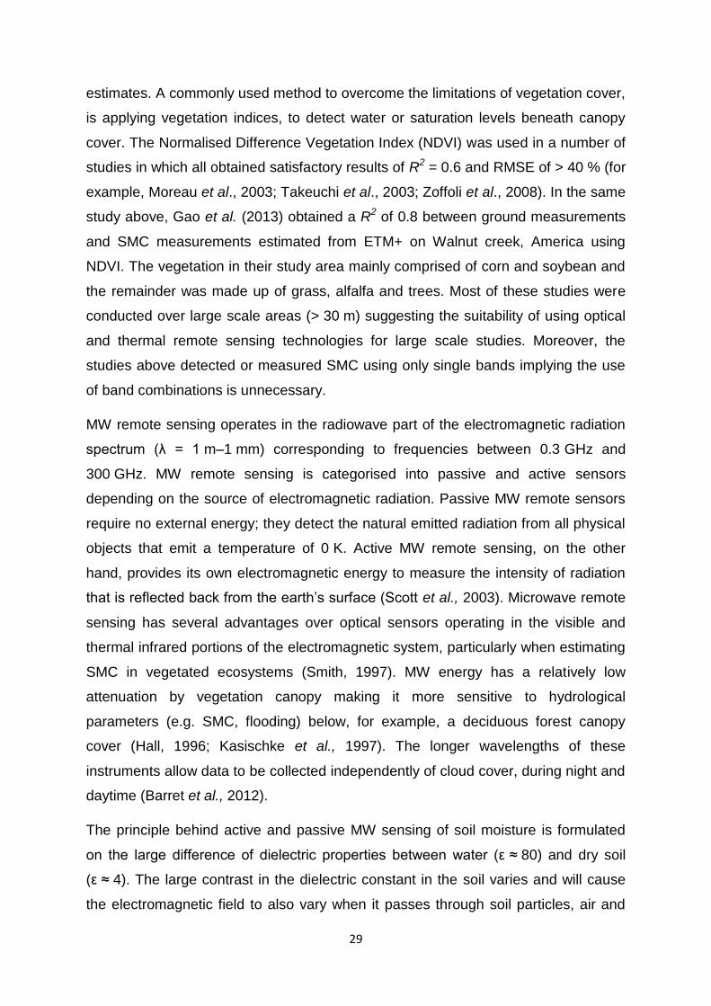
29
estimates. A commonly used method to overcome the limitations of vegetation cover,
is applying vegetation indices, to detect water or saturation levels beneath canopy
cover. The Normalised Difference Vegetation Index (NDVI) was used in a number of
studies in which all obtained satisfactory results of R2 = 0.6 and RMSE of > 40 % (for
example, Moreau et al., 2003; Takeuchi et al., 2003; Zoffoli et al., 2008). In the same
study above, Gao et al. (2013) obtained a R2 of 0.8 between ground measurements
and SMC measurements estimated from ETM+ on Walnut creek, America using
NDVI. The vegetation in their study area mainly comprised of corn and soybean and
the remainder was made up of grass, alfalfa and trees. Most of these studies were
conducted over large scale areas (> 30 m) suggesting the suitability of using optical
and thermal remote sensing technologies for large scale studies. Moreover, the
studies above detected or measured SMC using only single bands implying the use
of band combinations is unnecessary.
MW remote sensing operates in the radiowave part of the electromagnetic radiation
spectrum (λ = 1 m–1 mm) corresponding to frequencies between 0.3 GHz and
300 GHz. MW remote sensing is categorised into passive and active sensors
depending on the source of electromagnetic radiation. Passive MW remote sensors
require no external energy; they detect the natural emitted radiation from all physical
objects that emit a temperature of 0 K. Active MW remote sensing, on the other
hand, provides its own electromagnetic energy to measure the intensity of radiation
that is reflected back from the earth’s surface (Scott et al., 2003). Microwave remote
sensing has several advantages over optical sensors operating in the visible and
thermal infrared portions of the electromagnetic system, particularly when estimating
SMC in vegetated ecosystems (Smith, 1997). MW energy has a relatively low
attenuation by vegetation canopy making it more sensitive to hydrological
parameters (e.g. SMC, flooding) below, for example, a deciduous forest canopy
cover (Hall, 1996; Kasischke et al., 1997). The longer wavelengths of these
instruments allow data to be collected independently of cloud cover, during night and
daytime (Barret et al., 2012).
The principle behind active and passive MW sensing of soil moisture is formulated
on the large difference of dielectric properties between water (ε ≈ 80) and dry soil
(ε ≈ 4). The large contrast in the dielectric constant in the soil varies and will cause
the electromagnetic field to also vary when it passes through soil particles, air and

30
water in the soil (Walker, 1999). By measuring the strength of the signal in the MW
sensor, an amount of water content contained in the soil can be determined through
the soil’s dielectric properties (Schmugge, 1985; Engman and Chauhan, 1995).
However, it becomes a challenge when distinguishing whether the MW signal is
derived from the soil surface or from the actual soil water content itself. This is
because of the influence on the signal from the sensor (wavelength and
polarization), vegetation cover and surface roughness (Barret et al., 2012). For
example, the effects of vegetation cover on an active sensor’s backscatter signal
decreases with increasing wavelength (Figure 3). MW sensors used to retrieve SMC
are acquired in different wavelengths that range from X-band (λ = ~3 cm), C-band
(λ = ~5 cm) and L-band (λ = ~30 cm) (Moghaddam et al., 2000). Sensors with a
short wavelength (X-band = ~3 cm) are only able to penetrate into the top layer of
the soil surface unlike longer wavelength sensors (L-band = ~30 cm) which are able
to penetrate deeper into the soil surface (Wagner et al., 2006).
31
Figure 3:The shorter microwave wavelength (X-band, 3cm) interacts mostly with the top of the canopy cover, sensors with longer wavelengths (L-band, 24 cm) are able to further penetrate into the canopy and interact with the soil surface (adapted from Barrett and Petropoulos, 2012: 91)
Specific to retrieving SMC under vegetated areas, passive L-band MW sensors have
displayed the potential to be more robust compared to active C-band MW sensors
(Narvekar et al., 2015). This is due to the scattering and attenuation from vegetation
cover and surface roughness having very little influence on the lower frequency
backscatter (L-band) as compared to higher frequencies (C-band) backscatter signal
(Oveisgharan et al., 2018). Currently, two space missions such as European Space
Agency’s Soil Moisture and Ocean Salinity (SMOS) and National Aeronautical and
Space Administration’s (NASA) Soil Moisture Active Passive (SMAP) offer 40 km to
50 km spatial resolution imagery with a short two to three days revisit time (Wagner
et al., 2006). Various research studies relating L-band radar data to soil moisture
have been conducted, however, to date, most studies have focused on forests and
occasionally agricultural areas. For example, a recent study by Al-Yaari et al. (2014),

32
showed that L-band SMOS and C-band AMSR-E (spatial resolution of 25 km) were
able to capture the variability of SMC in different biomes, climatic regions and soil
conditions, spatially and temporally, although SMOS had better correlation values in
densely vegetated biomes (e.g. tropical and temperate humid) compared to AMSR-E
(R = 0.64 and R = 0.15, respectively). In a research study, Sanli et al. (2008)
regressed RADARSAT-1, ASAR and PALSAR estimated backscatter against in situ
soil moisture over Turkey. The results showed good accuracies of R2 = 0.76, 0.81
and 0.86, respectively. From these studies, it is evident that the L-band sensors are
most appropriate to estimate soil moisture under vegetated areas due to their
advantage of wavelength and penetration depth. However, L-band passive MW
sensors are characterised by broad spatial coverage, and course spatial resolutions
(from tens of kilometres) (Barret et al., 2012). Whilst this resolution is practical for
global terrestrial application, it is not sufficient for estimating small features in the
landscape and heterogeneous ecosystems, such as the palustrine wetlands in semi-
arid regions (Entekhabi et al., 1999; Crow et al., 2000; Piles et al., 2011). Palustrine
wetlands in South Africa are small in extent and require high spatio-temporal
resolution imagery in order to detect changes in SMC (Haas, 2016).
C-band data has been in operation since 1991 such as the European Remote
Sensing Satellites (ERS) (Lang and Kasischke, 2008). C-band backscatter coefficient
is mainly influenced by the scattering caused by canopy cover. This is due to the
length of the MW wavelength in relation to the size, orientation and density of canopy
that determines how deep the MW is able to penetrate (Lang and Kasischke, 2008).
This coupled with the sensor’s characteristics affects the MW transmission in dense
vegetation cover (Lang and Kasischke, 2008). For instance, vertically transmitted
and received (VV) MW energy is not able to readily penetrate through forests as
compared to horizontally transmitted and received (HH) MW energy. This is because
structures that are vertically orientated would interact more with the VV polarization
mode and attenuate the penetration. Therefore, the HH polarization mode would be
able to transmit through the vertically orientated structures and reach the surface
where hydrological parameters such as inundation or SMC can be detected,
particularly for biomass ≤ 1 kg/m2 (Hess et al., 1995; Wang et al., 1995; Lang and
Kasischke, 2008; Hornacek et al., 2018).

33
Once the polarization energy is transmitted through the canopy it is able to interact
with the surface, then the soil moisture can either increase double-bounce scattering,
volumetric scattering or eliminate surface scattering (Figure 4) (Wang et al., 1995;
Kasischke et al., 2003). Various studies investigated the response of backscatter to
soil moisture. For example, Dabrowska-Zielinska et al. (2016) showed that VH
obtained a better accuracy in estimating SMC with R² = 0.72 compared to VV with
R² = 0.63 over an area comprised of grasses and sedges, using Sentinel-1 sensor.
The results from another study done by Dabrowska-Zielinska et al. (2018)
investigated the response of single polarization modes and cross-polarization
modes, using Sentinel-1, at depths of 5, 10 and 20 cm over two types of vegetation
(marshland and grassland) in the Biebrza wetlands, Europe. The results show that
for the marshland area, the VH polarization mode achieved a Pearson’s correlation
(R) of 0.56; 0.46 and 0.59 and for the VV polarization mode, R = 0.55; 0.39 and 0.52.
For the grassland area the VH polarization mode achieved an R = 0.55; 0.53 and
0.47, while for the VV polarization mode R² = 0.72; 0.69 and 0.55. In conclusion,
using cross-polarization modes such as VH in general present higher coefficients of
determination for grassland type vegetation in wetlands due to its ability penetrate
the vegetation structure and interact with the soil surface.
Figure 4: Three types of scattering (transmit and receive signals) depending on target (Source: adapted and modified from: Bai et al. (2017a:186).
In summary, L-band sensors have the advantage of detecting soil moisture in highly
densely vegetated areas due to their longer wavelength and deeper penetration
properties. However, L-band sensors are limited by their coarse resolution for certain
34
sensors, for example SMOS; the revisit time, for example ALOS has a revisit time of
46 days; and the cost associated with acquiring the images, when it comes to
estimating SMC in features with small extents, such as palustrine wetlands of semi-
arid regions. The most common active remote sensor that has been tested to date,
for estimating SMC in grasslands is the C-band Synthetic Aperture Radar (SAR)
system (Wulf et al., 2015). This is likely linked to the fact that the Sentinel sensors
can provide imagery at a high spatial resolution of 10 m, making them more suited to
quantify and map SMC for smaller features (Zhang et al., 2017a). In order to monitor
the hydrological regime in palustrine wetlands, especially in a semi-arid country,
relatively high spatial resolution imagery is required at frequent revisit times. Since
S1 has proven success in other grasslands and palustrine wetlands, as per the
Dabrowska-Zielinska et al. (2018) and other studies, can it be used in South Africa
for improving the detection and monitoring of palustrine wetlands in the grassland
biome?
Sentinel-1A (S1A) which was launched on 3 April 2014 and Sentinel-1B (S1B) which
was launched on 25 April 2016, uses two C-band SAR satellites that operate in
Interferometric Wide Swath (IWS) mode with a high spatial resolution of 5 m x 20 m
which images a wide swath in dual polarization. This includes VV and VH
polarimetric modes. A few requirements for operational users include a high
temporal sampling rate, near-real-time data availability and free and easy access.
The temporal revisit time for S1 satellites is every five days, making it suitable for
detecting changes in the hydrological period. Sentinel-2A (S2A) was launched on the
23 June 2015 and is an optical space-borne sensor. Multispectral Instrument (MSI)
images are obtained in 13 spectral bands that range from visible, NIR to Short-wave
Infrared (SWIR). The first four bands (at 10 m spatial resolution) traditionally provide
information required for land cover classification; the next six bands (20 m spatial
resolution) meet the basic requirements for vegetation studies while the last three
bands (60 m spatial resolution) are used to measure atmospheric conditions (Drusch
et al., 2012). The advent of Sentinel-2B (S2B) on the 1 March 2017 implied an even
shorter revisit time to five days. This means that from all the mainstream freely
available satellites, to date, the Sentinel-2 series have the shortest revisit time.

35
In conclusion, a small number of studies have investigated the use of the Sentinel
sensors to estimate SMC for grasslands and palustrine wetlands. To my knowledge,
these include Dabrowska-Zielinska et al. (2016; 2018) in Europe; Bai et al. (2017b)
over the Tibetan Plateau; El-Hajj et al. (2017) in France; Holtgrave et al. (2018) in
Germany; and Möller (2014) in central region of Western Cape of South Africa. No
studies have been undertaken in the grassland biome of South Africa, there has
been no investigation of the use of Sentinel 1 and Sentinel 2 in palustrine wetlands in
the grassland biome of South Africa.

36
Chapter 3 : MATERIALS AND METHODS

37
3.1 Study area
3.1.1 Description of study area
The study area is situated primarily within and around the Colbyn Valley Nature
Reserve (CVNR) (25°44’30” S; 28°15’49” E), a municipal protected area of
approximately 20.8 Ha, located within the City of Tshwane Metropolitan Municipality
and the Gauteng Province of South Africa (Figure 5). The location of the CVNR is
positioned within the grassland biome of South Africa and more locally within a
residential urban area. The Hartebeesspruit River drains the catchment from the
head of the watershed and flows in a northerly direction up to a dolerite dyke. The
dolerite dyke forms a barrier on the northern side of the study area, and even though
it has been breached by the River, water backs up south of the dyke, resulting in the
formation of a channelled valley-bottom wetland. The restricted flow through the
breach and the seeps from the adjacent hillsides contribute interflow from the sides
contributing to the wetland (Grundling, 2015).
Most of the wetland remains permanently saturated throughout the hydroperiod and
coincide with the centre part of the wetland where peat have accumulated (extent
estimated at 4.68 Ha) (Delport, 2016). The peat is made up of medium fibrous reeds
and sedges and accounts for much of the water-holding properties. Highly organic
soils can be found in the permanently wet areas which display wetness
approximately 50 cm from the surface and show hydromorphic characteristics such
as mottling and high clay content (Venter et al., 2016).
The site is exposed to a number of pressures and impacts. Drainage has been
disrupted by numerous roads resulting in high energy runoff leading to erosion of the
wetland (Sherwill, 2015). Weirs have been built along the channel to alleviate the
effects of erosion in order to prevent further degradation of the wetland near the
Koedoespoort Railway line causing soil compaction which could induce flooding in
some areas, as well as altered drainage which could lead to a loss of recharge
(DEA, 2015). These affects have a consequence on the wetland’s soil moisture
regimes and plant species (Sherwill, 2015).

38
Figure 5: The location of the study area, the Colbyn Valley Nature Reserve (CVNR), is located within the Gauteng Province of South Africa (a). The CVNR hosts a channelled valley-bottom wetland (b) through which the Hartebeesspruit (River) runs. The location of sample plots is displayed in the wetland and terrestrial areas.

39
3.1.2 Climate
The study area is located within the Rocky Highveld region of the Grassland biome
which encounters a mean annual temperature of 12-20 °C (Kleynhans et al., 2005;
Mucina and Rutherford, 2006). Geographically, the area is located on the Highveld
Plateau between 1 335 m and 1 340 m above mean sea level and experiences a
temperate climate with the rainfall season between September and March and the
dry season between April and August. This ecoregion experiences an average
summer rainfall between 650 and 750 mm per annum (Figure 6) and an
evapotranspiration of 524 mm annually (ARC-ISCW, 2018).
Figure 6: Mean monthly precipitation for 2017 and 2018 (especially during sampling periods) according to the Station 30687 situated in Pretoria, South Africa (ARC-ISCW, 2018).
3.1.3 Vegetation
The CVNR is considered a palustrine wetland type which is dominated by a variety
of graminoids and sedges. The temporary saturated zones of the wetland are
predominantly grass species such as Imperata cylindrica, which gradually flows into
a sedge community under moister conditions, up to the permanently saturated zones
with Phragmites australis, Typha capensis and Carex acutiformis (Venter et al.,
2016). The area along the river channel known as the riparian zone is marked by
0
5
10
15
20
25
30
35
Jan Feb Mar Apr May June July Aug Sept Oct Nov Dec
Me
an m
on
thly
pre
cip
itat
ion
(m
m)
2017
2018

40
exotic riparian vegetation; most of which is in the form of trees (Salix babylonica) and
the remainder of the study area is covered with vegetation throughout the year
(Figure 7).
Figure 7: Vegetation found in the wetland area varying from Typha capensis to Imperata cylindrica during end of peak growing season (left and right, respectively).
3.2 Data collection
3.2.1 Image acquisition and pre-processing
Sentinel-1 SAR data acquisition and pre-processing
The Sentinel-1A (S1A) and Sentinel-1B (S1B) Synthetic Aperture Radar (SAR) C-
band images were acquired in the Interferometric Wide (IW) swath mode, at 5 m by
20 m spatial resolution. The images were downloaded from the Copernicus website
(https://scihub.copernicus.eu/dhus/#/home) (Table 3). The data were acquired in the
vertical-transmit, vertical-receive (VV) and vertical-transmit, horizontal-receive (VH)
polarization modes. S1A and S1B Ground Range Detected (GRD) data was pre-
processed using ESA’s Sentinel Application Platform software (SNAP) version 6.0
(2018) for radiometric calibration, multi-looking and terrain correction. Multi-looking
was applied to each Sentinel-1 image to convert a 10 m spatial resolution image to
20 m spatial resolution image to reduce the speckle present in the images.
Radiometric calibration of the Synthetic Aperture Radar (SAR) images converts the
data from a digital number (DN) format to backscatter in sigma naught or sigma dB.

41
Errors associated with terrain, orientation and geo-referencing of the imagery were
corrected with the Range Doppler Terrain Correction using the Shuttle Radar
Topography Mission 3 (SRTM 3) arc-seconds 30 m Digital Elevation Model (USGS,
2004).
Table 3: Acquisition dates and times of the Sentinel 1A/1B and Sentinel 2A/2B images as well as the dates of ground measurements.
Sensor Scene ID no. Date
(2018)
Time of
overpass of
sensor
(GMT+ 2 hrs)
Hydroperiod
S1A
S1A_IW_GRDH_1SDV_20180326T16
4655_20180326T164720_021188_02
46E
26 March 18:44 Peak
S1B
S1B_IW_GRDH_1SDV_20180328T03
3428_20180328T033453_010226_01
2958_A3E7
28 March 05:33 Peak
S2A L1C_T35JPM_A014432_20180328T0
81650 28 March 09:45 Peak
S2B L1C_T35JPM_A006024_20180502T0
81534 02 May 09:45 End
Sentinel-2 data acquisition and pre-processing
Sentinel-2 optical images were acquired as close as possible to the SAR images,
though avoiding imagery with > 20% cloud coverage. The images were downloaded
from the United States Geological Survey (USGS) Earth Explorer website (USGS,
2000) as ten individual spectral bands. Bands 2, 3, 4 and 8 are provided by ESA at a
10 m spatial resolution while bands 5, 6, 7, 8a, 11 and 12 are at 20 m spatial
resolution (Table 4). Bands with a 60 m spatial resolution (bands 1, 9 and 10) are
mainly used in atmospheric correction and cirrus-cloud screening and were not
required for estimating the percentage Soil Moisture Content (%SMC). Three
procedures were necessary for pre-processing the satellite images, (1) resampling
the 20 m multispectral images to 10 m to maintain an image with the same spatial
resolution and number of pixels. This higher spatial resolution image provides more
detail for data extraction and modelling, required at the level of palustrine wetlands;
(2) atmospheric correction, terrain and cirrus correction to Top-of-Atmosphere was

42
applied to each image using the iCOR plugin in SNAP and; (3) a subset selection
was applied to extract the study area.
Table 4: Spectral bands and associated wavelength ranges of the optical Sentinel 2A and 2B images (adapted from ESA Sentinel online, 2019).
S2A S2B
Spatial
Resolution
(m)
Band
Number
Central
Wavelength
(nm)
Bandwidth
(nm)
Central
Wavelength
(nm)
Bandwidth
(nm) Use
10
2 442.7 21 442.2 21 Aerosol correction,
Land measurement
3 492.4 66 492.1 66 Land measurement
4 559.8 36 559.0 36 Land measurement
8 664.6 31 664.9 31
Land measurement,
water vapour
correction
20
5 704.1 15 703.8 16 Land measurement
6 740.5 15 739.1 15 Land measurement
7 782.8 20 779.7 20 Land measurement
8a 832.8 106 832.9 106 Land measurement,
water vapour
11 864.7 21 864.0 22 Land measurement
12 945.1 20 943.2 21
60
1 1373.5 31 1376.9 30 Aerosol correction
9 1613.7 91 1610.4 94 Water vapour
correction
10 2202.4 175 2185.7 185 Cirrus detection
3.2.2 In situ soil moisture measurements
Prior to sampling, several field visits were made to plan sampling positions in the
wetland and terrestrial areas. The wetland and terrestrial areas were identified by
characterising the nature of the soil, extracted from the ground using a soil auger;
vegetation type such as the Typha capensis, Phragmities and Imperata Cylindrica;
as well as the National Wetlands Map 5 (NWM5). The duration of the sampling
period was selected to coincide with the peak hydroperiod, which would help to
detect the maximum level and extent of soil moisture in the wetland for wetland
inventorying. A stratified random sampling method was chosen to collect in situ,
percentage Volumetric Water Content (%VWC) measurements in the wetland and
the terrestrial areas. The reason for the stratified random sampling was to ensure the

43
point sample measurements are well distributed in order to represent the wetland
and terrestrial sampling areas. Previously dated Sentinel images were downloaded
and used to determine suitable positions for the sampling plots which were
positioned to match both the Sentinel SAR and optical image. Therefore, a sampling
plot the size of 10 m x 10 m was positioned within a 20 m x 20 m grid. There were
forty sampling plots in total, 20 located in the wetland area and 20 located in the
terrestrial area (Figure 5). For each sample plot, five replicate measurements of
%VWC were recorded in order to capture the variation of the observed %SMC within
the top layer of the soil surface (refer to Figure 8 for a representation of the sampling
plots and in situ sampling measurements). This yielded a total of 200 readings for
the terrestrial and wetland areas during each sampling campaign. The reason was to
guarantee that a single field plot will have a corresponding S1 and S2 extracted data
pixel.
Figure 8: Diagram illustrating the planning of sampling according to the Sentinel 1 and 2 image pixels. The smalls (green) squares represent the in situ sampling measurements that were specifically located with both Sentinel 1 and Sentinel 2 pixels (blue outline) to ensure values could be extracted for both sensor’s pixels.
Near-surface volumetric soil moisture content was acquired using a hand-held SMT-
100 soil moisture and temperature probe (Sichuan Weinasa Technology Co., Ltd.
2017). The probe measures the %VWC at a depth of 5 cm. The centre and corners
of each sample plot was mapped in ArcGIS version 10.5 (ESRI, 2016) and then
uploaded to several e-Trex 30 Global Positioning Systems (GPSs) (GARMIN, 2011).
The GPSs was then used to navigate to the same location for successive sampling
campaigns. Previous studies recommended that ground measurements should be
made within a two-hour window period around the sensor overpass time so as to
minimise diurnal variation in soil moisture content and vegetation on radar
backscatter (Möller, 2014; Baghdadi et al., 2015;). Therefore, three probes were

44
used by three teams, deployed to record the %VWC within a two-hour time period
around the satellite overpass, including the hour before and after the time of
overpass of each Sentinel sensor.
During the field campaigns, the vegetation height in various zones were randomly
measured and recorded. The height of the vegetation in the terrestrial area, for
example, comprised of short grasses with an average height of < 3 cm. The
vegetation in the wetlands zone ranged from sedges and graminoids to macrophytes
with an average height range between 1.5—2 m. The density and height of the
vegetation in both zones varied little for the duration of %VWC data collection
between March and May of 2018. The biomass of these grass and sedge
communities where sampling took place considered to be ≤ 850 g/m² (Naidoo et al.,
2019). According to Hornacek et al. (2018), vegetation and texture have very little
impact on the %SMC modelling if grass vegetation is ≤ 1 kg/m2. Consequently, no
adjustments were made for vegetation or texture in the regression models used.
3.3 Data analysis
In order to assess the Sentinel sensor’s capability to estimate the %SMC,
backscatter from Sentinel-1A and 1B (S1A and S1B) and reflectance values for
Sentinel-2A and 2B (S2A and S2B) were extracted from the respective images and
regressed against the in situ %VWC measurements. The centre point recorded for
each sample plot in shapefile format were used to extract backscatter values for VV,
VH polarization modes as well as VV+VH as a modelling scenario, in ArcMap 10.5
(ESRI, 2016). Similarly, the spectral reflectance values of the optical sensors were
extracted for all the bands, excluding bands 1, 9 and 10 (60 m resolution bands),
individually as well as the combination of them, for the same points.
Factors such as precipitation, evapotranspiration, soil compaction and reflectance
can influence the distribution of %SMC (Lu et al., 2001). Therefore, the distributions
of the in situ %VWC measurements were tested first for normality. By performing a
normal-distribution graph in order to visualise the nature of the in situ data, one can
determine whether parametric and non-parametric models are appropriate for
assessing the senor’s capability to estimate %SMC. The principle behind the
parametric approach is that the model assumes normal distribution of the data, and

45
therefore depends on mean and standard deviation statistics, whereas non-
parametric analysis does not assume normal distribution. Spectral data is often
found to be not normally distributed, and hence non-parametric approaches have
previously been found to outperform the parametric approaches in remote sensing.
Parametric models repetitively selects features, randomly, which is then used in the
regression, and the procedure is repeated with the remaining features in
bootstrapping. This process continues until the combinations within the dataset are
exhausted. The features are rejected and ranked accordingly and this will then
provide the best results in terms of estimation accuracy (Ali et al., 2015). Parametric
models, such as simple linear regression, are simple and less complex in terms of
tuning, but they use only a fixed number of input variables and thus can only be used
if the data is assumed to be normally distributed.
Non-parametric analyses produce a model of multidimensional and non-linear
relationships between the target (%SMC) and input variables (Attarzadeh et al.,
2018). Unlike parametric models, the number of input variables in non-parametric
models is flexible and changes as it learns from the data and it makes fewer
assumptions about the data (Ali et al., 2015). This study could significantly gain from
using non-parametric models due to its ability to undertake small training databases
in order to perform a strong SMC retrieval. Ahmed et al. (2010) conducted a time
series analysis from 1998-2005 using the Advanced Very High Resolution
Radiometer (AVHRR). A Support Vector Machine (SVM) algorithm was employed to
estimate %SMC on 10 sites comprised of low to dense vegetation, of which five
years was used as the training dataset and the remaining three years was used to
test the model. The correlation coefficients for the estimated %SMC ranged from
0.34 – 0.77 with an RMSE < 2% for all of the study sites, indicating the capability of
the SVM model to capture the variability of measured %VWC. Several studies
showed capabilities of both parametric and non-parametric approaches in estimating
%SMC from both SAR and optical data with ranges of accuracies. In this study, both
approaches were tested to assess whether any differences were noted in the results.
The S1 backscatter values and S2 reflectance band values were regressed against
the %VWC values (in situ measurements) using both parametric (Simple Linear
Regression model or SLR) and non-parametric (SVM, Random Forest or RF)
algorithms in the Waikato Environment for Knowledge Analysis (Weka) software
46
version 3.8 (Eibe, 1999-2016). In another study, Srinivaso Rao et al. (2013)
estimated %SMC using the modified Dubois Model (parametric model) over the
agricultural lands in the region of India. The results were validated against in situ
%VWC measurements. Their poorest fit was a correlation (R2) of 0.46 over a densely
vegetated area, R2 = 0.5 was achieved over an area where the vegetation had
reached the matured stage and the highest accuracy achieved was R2 = 0.77 over
an area with sparse vegetation with a mean height of 10 cm. Overall they obtained a
RMSE of < 4.31 %. Their poorest fit was attributed to the intense vegetation
coverage and heavy rainfall prior to sampling. Therefore, the differences in
accuracies suggest that retrieving SMC if the data is normally distributed, i.e. no
dense vegetation cover or heavy rainfall periods prior or during sampling periods, the
use of parametric models would be appropriate.
A data split was used with 30 % data for the training dataset and 70 % for the
validation dataset to test the best model for regressing the observed %VWC to the
estimated %SMC. In addition to the data split approach, a cross-validation procedure
was also performed to evaluate the best-fitting models. The purpose of including the
cross-validation method is because it is appropriate for scenarios where the dataset
may be too small. Individual polarizations and bands, as well as a combination of the
polarizations and all bands have been evaluated for each sensor in predicting
%SMC. The sensor, algorithm and variables which can predict %SMC with the
highest coefficient of determination (R²) and lowest the Root Mean Square Error
(RMSE) were considered the best to use for producing a predicted %SMC map for
each of the Sentinel (SAR and optical) sensors (Figure 9).

47
Figure 9: Flowchart illustrating the different stages of the overall procedure and methodology to generate the final outcome of a predicted percentage Soil Moisture Content (%SMC) maps.
Data from both the in situ %VWC measurements and predicted %SMC maps were
used to assess the differences in SMC. The 200 points collected across wetland and
terrestrial areas were used to test a significant difference by conducting a Welch two
sampled t-test in RStudio version 1.1.456 (Rstudio, Inc., 2009-2018) at a 95%
confidence interval. If significant differences between these plots were found, a
threshold of %SMC could be selected to distinguish the wetland extent from the
terrestrial extent. For wetland mapping, the criteria used to set a threshold were
based on the principle of mapping the maximum extent of soil saturation of the
wetland across multiple hydroperiods (Van Deventer et al., 2018b). Following the
examples of thresholds discussed in Chapter 2, it is likely that a threshold close to
±45 %VWC can be used to determine the extent of terrestrial area and ±50 %VWC
can be used to determine the extent of wetland area based on studies conducted
over grasslands done by Paloscia et al. (2013) and Holtgrave et al. (2018). In this
study, a threshold was chosen based on the average mean %VWC across the
terrestrial and wetland areas, however, were informed by a single season sampling
to demonstrate the concept. The threshold were then applied to the predicted %SMC
map and compared to the extent of the wetlands digitised by wetland experts in the
National Wetland Map version 5 (NWM5) (Van Deventer et al., 2018b). The extent of

48
agreement and differences in wetland extent, in terms of their percentage of the
extent of the study area, were explored between these two datasets to inform
wetland inventorying.

49
Chapter 4 : RESULTS

50
4.1 Descriptive statistics analysis and normality testing for in
situ volumetric water content measurements
The maximum percentage Volumetric Water Content (%VWC) was measured at
100 % while the minimum was measured at 4.5 % (Table 5). The range illustrates
the spatial distribution of soil moisture across terrestrial and wetland areas for March
and May 2018. Although there is noticeable variation across the study site, the
standard deviation as a function of soil moisture indicates a relatively wide variability
at 37 %. The distribution of the in situ %VWC measurements and the estimated
percentage of Soil Moisture Content (%SMC) was not normally distributed (Figure
10). The non-normality was caused by the skewness to the right for in situ %VWC
measurements measured on the 28 March 2018 and skewed to the left for in situ
measurements at the time of the Sentinel-2B overpass on the 2 May 2018.
Table 5: Descriptive statistical analysis illustrating the variability of soil moisture across the study site during the March and May 2018 sampling campaigns
Observed percentage of Volumetric
Water Content (%VWC)
Number of samples (in total for 28 March 2018 and 2 May 2018 sampling campaigns)
400
Mean 61
Minimum 4.5
Maximum 100
Standard Deviation 37
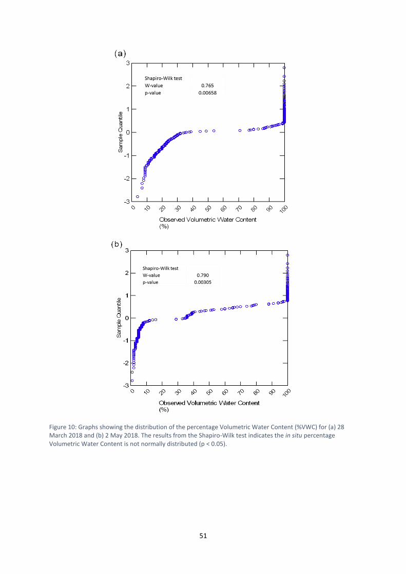
51
Figure 10: Graphs showing the distribution of the percentage Volumetric Water Content (%VWC) for (a) 28 March 2018 and (b) 2 May 2018. The results from the Shapiro-Wilk test indicates the in situ percentage Volumetric Water Content is not normally distributed (p < 0.05).

52
4.2 Ability of Sentinel-1 and Sentinel-2 to estimate soil moisture
content
The Sentinel sensors were capable of predicting the %VWC with correlation
coefficients (R2) > 0.7 and RMSEs < 17 %. Of the four sensors, Sentinel-1B (S1B)
produced a high correlation coefficient (R2) of 0.92—0.94 and the lowest Root Mean
Square Error (RMSE) of 10 %. Sentinel-2B (S2B) achieved the second-highest
results with an R2 of 0.92—0.94 and RMSE of 12 %-14 %. Sentinel-2A (S2A)
produced slightly better results (R2 = 0.8—0.86; RMSE = 15 %—16 %) than Sentinel-
1A (S1A) which resulted in the lowest R2 of 0.76—0.8 and highest error at RMSE =
13 %—17 % (Table 6).
Of the three polarization modes (vertical-receive, vertical-transmit (VV); vertical-
receive, horizontal-transmit (VH); and VH+VV associated with the two Sentinel-1
(SAR) sensors the VH polarization mode and the VH+VV modelling scenario yielded
higher accuracies (R² > 0.72) and lower errors (RMSE < 19 %) compared to the VV
polarization (Table 6). S1B showed the highest coefficient of determination (R² > 0.9)
when the VH polarization and VH+VV modelling scenario were used, with an RMSE
of 10 % in both instances. The results for S1A were slightly lower at R2 = 0.79 and a
slightly higher RMSE of 13 % for VH and 16 % for VH+VV modelling scenario. The
single VV polarization showed the lowest coefficient of determination and highest
error (R2 = >0.2; RMSE = >35 %) for both of the Sentinel-1 sensors. The VH
polarization mode, however, contributes more to the accuracies of the combined
VH+VV modelling scenario inputs than the single polarization (VV) mode.
A combination of all the bands for the optical sensors S2A and S2B, in general,
resulted in high accuracies (R² > 0.7 and RMSE < 20%) across algorithms and
validation approaches (Table 6). Some exceptions are evident where the use of the
blue, green, red and vegetation red edge (VRE) bands produced comparable results
to the combined bands, most noticeably when the RF algorithm is used (R² = 0.8 for
S2A, or even higher for S2B (R² > 0.84). Five of the individual bands resulted in high
coefficient of determinations in estimating %SMC (R2 = >0.9; RMSE = 12%), namely,
blue (band 2:496–492 nm), green (band 3: 560–559 nm), red (band 4: 664–665 nm),
NIR (band 8: 833–835 nm) and SWIR (band 12: 2185–2204 nm).

53
When comparing the modelling approaches, the non-parametric Random Forest
(RF) algorithm outperformed the parametric Simple Linear Regression (SLR) and
non-parametric Support Vector Machine (SVM). RF achieved ranges of the
coefficients of determination from R² = 0.58 to R² = 0.94 and RMSE values between
10 % and 24 % (Table 6). In contrast, SVM had lower accuracies ranging from R² =
0.01 to R² = 0.66 and RMSE values between 24 % and 50 %. The SLR algorithm
showed similar ranges of coefficients of determination to that of the non-parametric
SVM algorithm (from R² = 0.01 to R² = 0.6) and RMSE values ranging from 29 % to
40 %. The data split method, in general, showed better results (R² = ≥ 0.1;
RMSE = ≤ 41 %) as compared to the cross validation method (R² = > 0.5;
RMSE = ≤ 50 %).
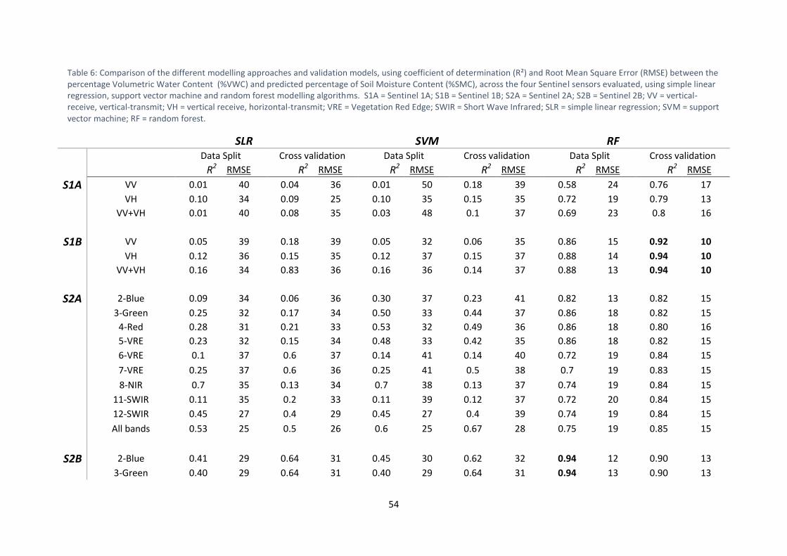
54
Table 6: Comparison of the different modelling approaches and validation models, using coefficient of determination (R²) and Root Mean Square Error (RMSE) between the percentage Volumetric Water Content (%VWC) and predicted percentage of Soil Moisture Content (%SMC), across the four Sentinel sensors evaluated, using simple linear regression, support vector machine and random forest modelling algorithms. S1A = Sentinel 1A; S1B = Sentinel 1B; S2A = Sentinel 2A; S2B = Sentinel 2B; VV = vertical-receive, vertical-transmit; VH = vertical receive, horizontal-transmit; VRE = Vegetation Red Edge; SWIR = Short Wave Infrared; SLR = simple linear regression; SVM = support vector machine; RF = random forest.
SLR
SVM
RF
Data Split Cross validation Data Split Cross validation Data Split Cross validation
R2
RMSE R2 RMSE R2
RMSE R2 RMSE R2
RMSE R2 RMSE
S1A VV 0.01 40 0.04 36 0.01 50 0.18 39 0.58 24 0.76 17
VH 0.10 34 0.09 25 0.10 35 0.15 35 0.72 19 0.79 13
VV+VH 0.01 40 0.08 35 0.03 48 0.1 37 0.69 23 0.8 16
S1B VV 0.05 39 0.18 39 0.05 32 0.06 35 0.86 15 0.92 10
VH 0.12 36 0.15 35 0.12 37 0.15 37 0.88 14 0.94 10
VV+VH 0.16 34 0.83 36 0.16 36 0.14 37 0.88 13 0.94 10
S2A 2-Blue 0.09 34 0.06 36 0.30 37 0.23 41 0.82 13 0.82 15
3-Green 0.25 32 0.17 34 0.50 33 0.44 37 0.86 18 0.82 15
4-Red 0.28 31 0.21 33 0.53 32 0.49 36 0.86 18 0.80 16
5-VRE 0.23 32 0.15 34 0.48 33 0.42 35 0.86 18 0.82 15
6-VRE 0.1 37 0.6 37 0.14 41 0.14 40 0.72 19 0.84 15
7-VRE 0.25 37 0.6 36 0.25 41 0.5 38 0.7 19 0.83 15
8-NIR 0.7 35 0.13 34 0.7 38 0.13 37 0.74 19 0.84 15
11-SWIR 0.11 35 0.2 33 0.11 39 0.12 37 0.72 20 0.84 15
12-SWIR 0.45 27 0.4 29 0.45 27 0.4 39 0.74 19 0.84 15
All bands 0.53 25 0.5 26 0.6 25 0.67 28 0.75 19 0.85 15
S2B 2-Blue 0.41 29 0.64 31 0.45 30 0.62 32 0.94 12 0.90 13
3-Green 0.40 29 0.64 31 0.40 29 0.64 31 0.94 13 0.90 13

55
4-Red 0.34 31 0.56 33 0.34 30 0.56 34 0.94 12 0.90 13
5-VRE 0.30 31 0.55 33 0.30 31 0.50 36 0.92 13 0.90 13
6-VRE 0.25 32 0.50 34 0.25 33 0.48 36 0.92 13 0.90 13
7-VRE 0.18 34 0.44 36 0.18 34 0.41 37 0.92 14 0.90 13
8-NIR 0.09 36 0.29 38 0.09 36 0.30 39 0.94 14 0.90 13
11-SWIR 0.36 30 0.59 32 0.36 31 0.59 33 0.92 14 0.90 13
12-SWIR 0.42 28 0.64 30 0.42 29 0.66 32 0.94 13 0.90 13
All bands 0.36 30 0.64 30 0.45 30 0.66 32 0.94 12 0.90 12

56
4.3 Differences in soil moisture content between wetland and
terrestrial ecosystem types
The in situ %VWC and predicted %SMC values derived from S1B and S2B showed
significant differences (p < 0.05) between the wetland and terrestrial areas (Table 7).
On 28 March 2018, higher levels of soil moisture ranging from > 60 % were observed
in the wetland sampling area and a lower range of soil moisture, less than ±30 %
(rounded off to the nearest 10th digit) were observed in the terrestrial sampling area
(Figure 11a). Similarly, a higher range of soil moisture levels occurred in the wetland
sampling area (> 45 %) as compared to the terrestrial sampling area (< ± 45 %) for
both the in situ %VWC and predicted %SMC of 2 May 2018 (Figure 11b). There is a
much larger variability between the in situ %VWC measurements as compared to
predicted %SMC measurements.
Table 7: Differences between the wetland and terrestrial areas for in situ percentage Volumetric Water Content (%VWC) and Soil Moisture Content (%SMC) resulting from the Sentinel 1B and 2B predictions.
Date In situ measurements Sensor Predicted soil moisture
measurements
28 March 2018 0.0000000000000023 Sentinel-1B 0.0000000000000027
2 May 2018 0.0000000000000024 Sentinel-2B 0.0000000000000029
Figure 11: Percentage Volumetric Water Content and predicted percentage of Soil Moisture Content levels between drylands and wetlands for (a) 28 March 2018 and (b) 2 May 2018.

57
The coefficient of variation (COV) and mean values for in situ observed %VWC for
the wetlands sample plots were low for the 28 March 2018 (COV = 1.2; mean = 90.7)
and high for the in situ sampling period on the 2 May (COV = 5.6; mean = 74.3).
Whereas, in comparison to the in situ %VWC, the COV and mean values for S1B
predicted SMC Values (COV = 0.7; mean = 80.7) and S2B predicted SMC
(COV = 0.05; mean = 51.9) were low. The coefficient of variation (COV) and mean of
the %VWC values measured for the terrestrial areas are low for both those
corresponding to the dates on which S1B (COV = 1.7; mean = 20.3) and S2B
(COV = 2.2; mean = 5.8) were acquired, whereas COV and mean values of the
predicted SMC values for S1B (COV = 0.6; mean = 23.3) and S2B
(COV = 2.3; mean = 28.6) were relatively high in comparison (Table 8).
The maximum %VWC was recorded as 100% for in situ measurements on 28 March
2018 at 05:33. The mean modelled %SMC for S1B (mean±standard
deviation = 80.7±21.4;23.3±7.5) compares well with the observed mean %VWC
(mean±standard deviation = 90.7±20.8;20.3±7.9) in the wetland and terrestrial areas,
respectively (Table 8). The S2B predicted SMC map was unable to model very high
values (close to 100) that had been recorded during the sampling date (Table 8).
Since S1B and S2B produced the best results, predicted SMC maps were generated
for the two sensors using the data-split method. The maximum observed %VWC
and/or modelled %SMC in the terrestrial area is less than 50 %VWC, which are
therefore suggested as the threshold for mapping wetland extent (Figures 12 and
13). The predicted %SMC maps for the S1B and S2B sensors show a distinct
difference in the extent of soil saturation. The SMC map predicted from SAR VH
taken on 28 March 2018 at 05:33 overpass, showed that 41 % (28,5 Ha) of the
extent of the study area could be wetland (Figure 12), with %SMC values below the
chosen threshold value of 50 % predicted %SMC. The S2B SMC map, in contrast,
indicated a larger extent of wetland area (approximately 72 % or 50,3 Ha) with the
predicted SMC values > 50 % (Figure 13). S1B shows relatively high SMC values
around the south of Hartebeesspruit River and along the railway lines whereas S2B
show higher SMC values (50 %—100 %) indicating more soil saturation.
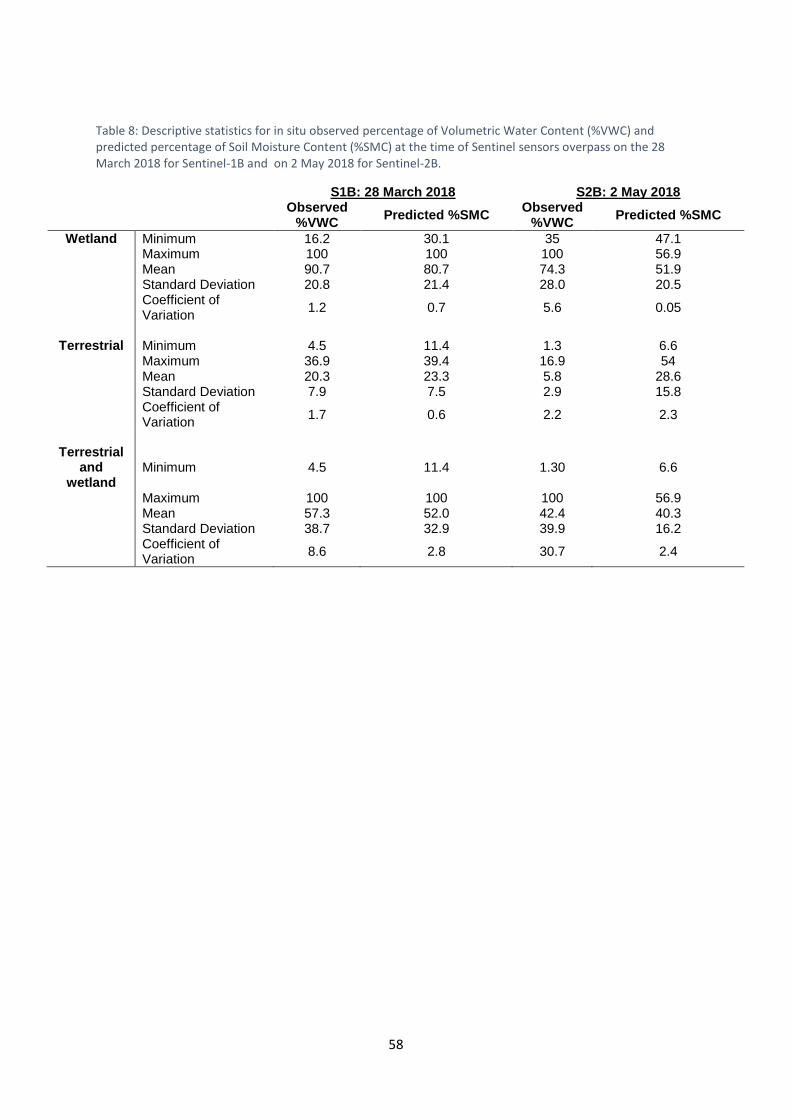
58
Table 8: Descriptive statistics for in situ observed percentage of Volumetric Water Content (%VWC) and predicted percentage of Soil Moisture Content (%SMC) at the time of Sentinel sensors overpass on the 28 March 2018 for Sentinel-1B and on 2 May 2018 for Sentinel-2B.
S1B: 28 March 2018 S2B: 2 May 2018
Observed %VWC
Predicted %SMC Observed
%VWC Predicted %SMC
Wetland Minimum 16.2 30.1 35 47.1
Maximum 100 100 100 56.9
Mean 90.7 80.7 74.3 51.9
Standard Deviation 20.8 21.4 28.0 20.5
Coefficient of Variation
1.2 0.7 5.6 0.05
Terrestrial Minimum 4.5 11.4 1.3 6.6
Maximum 36.9 39.4 16.9 54
Mean 20.3 23.3 5.8 28.6
Standard Deviation 7.9 7.5 2.9 15.8
Coefficient of Variation
1.7 0.6 2.2 2.3
Terrestrial
and wetland
Minimum 4.5 11.4 1.30 6.6
Maximum 100 100 100 56.9
Mean 57.3 52.0 42.4 40.3
Standard Deviation 38.7 32.9 39.9 16.2
Coefficient of Variation
8.6 2.8 30.7 2.4

59
Figure 12: Predicted percentage Soil Moisture Content (%SMC) map derived from Sentinel-1B showing the variation in soil moisture on 28 March 2018 sampling campaign.

60
Figure 13: Predicted percentage Soil Moisture Content (%SMC) map derived from Sentinel-2B showing the variation in soil moisture for 2 May 2018 sampling campaign.
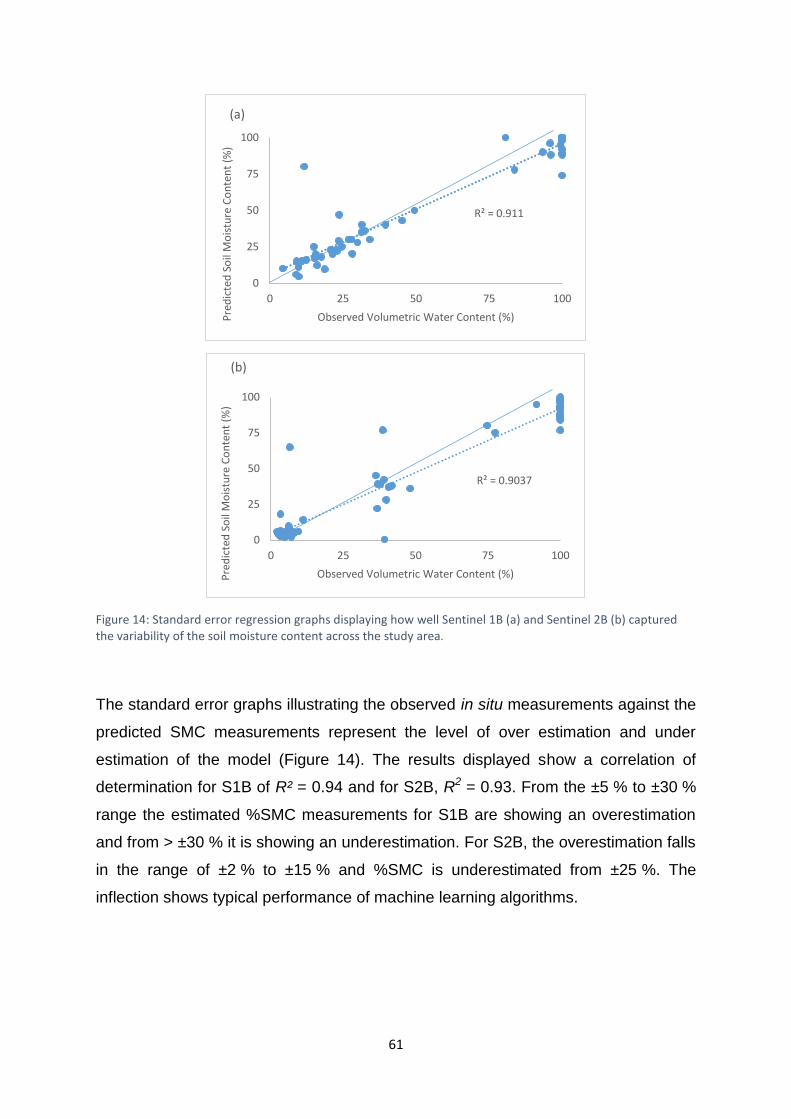
61
Figure 14: Standard error regression graphs displaying how well Sentinel 1B (a) and Sentinel 2B (b) captured the variability of the soil moisture content across the study area.
The standard error graphs illustrating the observed in situ measurements against the
predicted SMC measurements represent the level of over estimation and under
estimation of the model (Figure 14). The results displayed show a correlation of
determination for S1B of R² = 0.94 and for S2B, R2 = 0.93. From the ±5 % to ±30 %
range the estimated %SMC measurements for S1B are showing an overestimation
and from > ±30 % it is showing an underestimation. For S2B, the overestimation falls
in the range of ±2 % to ±15 % and %SMC is underestimated from ±25 %. The
inflection shows typical performance of machine learning algorithms.
R² = 0.911
0
25
50
75
100
0 25 50 75 100
Pre
dic
ted
So
il M
ois
ture
Co
nte
nt
(%)
Observed Volumetric Water Content (%)
(a)
R² = 0.9037
0
25
50
75
100
0 25 50 75 100
Pre
dic
ted
So
il M
ois
ture
Co
nte
nt
(%)
Observed Volumetric Water Content (%)
(b)

62
Chapter 5 : DISCUSSION
63
The results showed that C-band Synthetic Aperture Radar (SAR) Sentinel-1 (S1) and
optical sensor, Sentinel-2 (S2), were able to estimate soil moisture content (SMC) for
a palustrine wetland in the grassland biome of South Africa. S1 produced a high
correlation coefficient of R2 = > 0.76 and a low Root Mean Square Error (RMSE = <
24 %) and S2 produced an accuracy of R2 = 0.8 and low RMSE of < 20 %. Several
studies have made use of C-band to estimate SMC. A study by Dabrowska-Zielinska
et al. (2018) used the ERS-1/2 SAR VV and ENVISAT to monitor SMC over the
Bierbza wetlands in northeast Poland, cover by grassland and marshland. Their
findings show a reasonable error (RMSE) of 10 %. Holtgrave et al. (2018) estimated
soil moisture using the Sentinel-1 data in grassland floodplain Peene and Elbe,
Germany. The results showed high accuracies of R2 = > 0.72 and average RMSE of
13 % over the two sites. In another study conducted in the plains of Italy in a semi-
arid region, RADARSAT-2 estimated SMC with really high accuracies of R2 = 0.85
(Filion et al., 2015). In a recent study, Sadeghi et al. (2017) estimated soil moisture
using S2 over a watershed in Southern Arizona, in which low estimation errors of
0.04 cm3 cm-3 were derived. The results of this study therefore compares well in
terms of the coefficient of determination, though higher RMSE percentages were
recorded to all these comparable studies. All of these studies were conducted in
temperate climatic regions or over areas with grassland cover, and some include
palustrine wetlands which demonstrate that the C-band SAR sensors are capable of
predicting %SMC. This study shows that the freely available Sentinel-1 and optical
Sentinel-2 remote sensors can also estimate near surface SMC, to a depth of 5 cm,
for palustrine wetlands in the grassland biome of a semi-arid region.
A significant difference (p < 0.05) in soil moisture ranges was observed between the
wetland and terrestrial areas. In situ percentage Volumetric Water Content %VWC
ranged from 4.5 % to 100 %, while predicted %SMC ranged from 1.3 % to ±50 %.
The results showed that the mean soil moisture levels for the in situ %VWC
measured in the wetland (90.7 %; 74.3 %) was significantly higher (p < 0.05)
compared to the mean %VWC measured in the terrestrial area (20.3 %; 5.8 %) on
the 28 March and 2 May 2018, respectively. Similarly, the Sentinel sensors (S1B and
S2B) were able to pick up similar trends. Continuous assessment of the different soil
moisture ranges over multiple hydrological regimes would provide insight into
determining the maximum extent of a wetland (Van Deventer et al., 2018b). In this

64
study 50 % of the measured %VWC or predicted %SMC is suggested as a possible
threshold for determining the maximum extent of a wetland. Other studies such as
Holtgrave et al. (2018) measured %VWC ranging between ±30—99.1 % with a mean
value of close to 50 % of over a floodplain made up of grassland also reaching up to
2 m in height, in Germany. In another study, Paloscia et al. (2013) acquired %VWC
measurements with a mean of 45 % in terrestrial lands comprised of dense grasses,
in Italy. Both these studies took place at the end of the growing period of the
vegetation. In another instance, a study conducted by Lang et al. (2007) in the
coastal plains of Washington D.C. (United States of America), also attained similar
trends in the differences in the soil moisture ranges between the wetland and the
terrestrial area, with an average of 59 % and 24 % (%VWC), respectively. It appears
that these ranges have a similar trend, although in different biomes and regions. In
addition, for the Colbyn Valley Nature Reserve (CVNR) study area, on-site variation
in SMC values may be attributed to a number of factors. The vegetation in the
wetland area causes a decrease in velocity of flow due to the water holding capacity
of the plants as well as their high friction value. Also, the nature of palustrine type
wetlands is relatively flat which naturally decreases the velocity of flow, even if there
was no vegetation present at the time of sampling and overpass of the sensor
(Enviroguard Ecological Services cc. 2014). Other factors include sub-surface
fractures, groundwater flow, or alterations which have resulted in the accumulation of
water. As a result of the build-up of SMC in the valley-bottom, patterns of high SMC
across the wetland has in some instances linear appearances (marked 1 and 2 in
Figure 13), following old drains. In addition, the construction and filling of the area for
the road and railway line may have caused accumulation of water adjacent to these
areas (Figure 5).
Differences between the two sampling campaigns of this study in the CVNR may
relate to changes in the hydrological period. The sampling campaign on 28 March
2018 took place shortly after an intense rainfall storm (22 March 2018) whereas the
sampling campaign on 2 May 2018 took place approximately two weeks after a less
intense rainfall period (Figure 15). Despite the fact that the first campaign (28 March
2018) took place soon after an intense storm, the extent of soil saturation was much
wider (30 % or 21 Ha) from the image derived on 2 May 2018 associated with the
second campaign. The continuous rainfall events over summer (rainfall started mid-

65
February of 2018) lead to progressively accumulated water in the wetland through
surface run-off and groundwater accumulation. The accumulation of water would
have resulted in an increase dielectric constant, resulting in higher backscatter and
reflectance values. These results are evidence from the comparison of the predicted
SMC maps for S1B sensor and S2B sensor to one another, which suggests that
changes in soil saturation could be detected across the wetland’s hydroperiod. This
study, however, was limited to an inter-annual analysis at the peak and end of the
rainfall season and respective hydroperiod, limiting full understanding of the variation
of %SMC over the hydroperiod and extent of the wetland. Since palustrine wetlands
are dynamic ecosystems, they require frequent monitoring. Very high spatial (~ 1.2
m) and temporal resolution (1 – 3 days) imagery from WorldView or IKONOS, for
example, are most suitable for such an application, however, acquiring information
from these remote sensing platforms comes at a high cost which makes them
insufficient for regional monitoring of SMC. The Sentinel series surpasses this
limitation by offering freely available imagery with a relatively low revisit time of 5 – 6
days.
Figure 15: Precipitation readings for the duration of the sampling period. Graphs (a) shows a rainfall period shortly before
the acquisition for S1B on the 28 March 2018 (indicated by red arrow) and graph (b) shows the S2B acquisition on 2 May2018 (indicated by red arrow). Scale ranges are different to account for differences in the maximum precipitation of the two sample dates.
The estimated %SMC based on the interpretation from Sentinel-1 recorded in the
cross-polarization mode, found vertical-receive, horizontal-transmit (VH) to be more
sensitive to vegetation cover, surface roughness and SMC (R2 = 0.79; RMSE = 13
for S1A and R2 = 0.94; RMSE = 10 for S1B) compared to the single polarization
mode, vertical-receive, vertical-transmit (VV) (R2 = 0.76; RMSE = 17 for S1A and
R2 = 0.92; RMSE = 10 for S1B) and the VV+VH modelling scenario obtained the

66
same result as the VH polarization mode. The CVNR showed comparable results,
recommending the use of VH above that of VV. For instance, Dabrowska-Zielinska
et al. (2016) found that VH was able to estimate SMC with a higher accuracy (R2 =
0.72) than VV (R2 = 0.63) over a vegetated wetland area comprising of sedges,
reeds and grasses. By using the cross-polarization VH as well as integrating it into
the VV+VH modelling scenario, it was assumed that the influence from the
vegetation cover and surface roughness was reduced and the possibility of receiving
backscatter from the soil surface was increased.
The combination of all the optical S2 bands, resampled to 10 m spatial resolution
(excluding the 60 m spatial resolution bands), produced high accuracies of predicting
%SMC (R2 = > 0.7; RMSE = ≤ 15 %). S2B stacked bands showed the highest R2
(0.94) with the lowest RMSE (12 %). The accuracy in the %SMC estimation is
probably enhanced by the contribution of the visible range bands (blue (496–
492 nm), green (560–559 nm), red (664–665 nm)), the NIR (band 8, 833–835 nm)
and the SWIR (band 12, 2185–2204 nm), where the spectrum in these bands were
absorbed by water molecules, based on the results of the random forest’s (RF)
model ranking of the bands. These bands also produced a high R2 = 0.94 and low
RMSE = 13 %. Various other studies found that surface soil moisture the NIR and
SWIR was important for predicting soil moisture (Barret et al., 1993; Lobell and
Asner, 2002; Wang et al., 2009). For the CVNR, the use of bands across the visible,
NIR and SWIR all contributed to the optimisation of the prediction of %SMC.
The findings of our study indicated that non-parametric models (Support Vector
Machine (SVM) and RF) produced a better outcome as compared to the parametric
model (Simple Linear Regression (SLR)). The results from the Shapiro-Wilk test
indicate the in situ %VWC for the 28 March and 2 May 2018 sampling campaigns
are not normally distributed (w < 0.8; p < 0.05) (Figure 10 (a) and (b)). These results
are in agreement with other studies which also found non-parametric algorithms to
outperform parametric algorithms. For example, Ali et al. (2015) made a
comprehensive comparison between different machine learning methods and
concluded that non-parametric models such as SVM or Artificial Neural Network
(ANN) have great potential for measuring SMC for vegetated environments because
they require less amounts of training data. Liu et al. (2017) compared four different
machine learning approaches for observing monthly SMC satellite data over grain

67
crop regions in northeast China. They found that of all the four methods, RF showed
to have produced the best results with R2 generally greater than 0.92 (RMSE = 0.009
m3m-3). Cross-validation can be used when the number of samples doesn’t capture
the variability of the data. It appears as if the number of samples used in this study
did capture the variability and therefore where the data split was used, the results
were generally higher than the cross-validation approach.
Despite vegetation canopy cover influencing backscatter from C-band data, in this
study it can be argued that the vegetation may have very little impact on the radar
signal from C-band Sentinel-1 SAR. Several studies have attempted to compensate
for the influence of vegetation and surface roughness through incorporating it in their
models. Some methods included using sensors at different frequencies, polarization
modes and incident angles and assessing temporal variations across a part of the
phenological period when the biomass and texture remained the same (Zribi and
Dechambre, 2002; Baghdadi, et al., 2008; Paloscia et al., 2013). The most
commonly used index for incorporating the influence of vegetation in the estimation
of SMC, is the Normalization Difference Vegetation Index (NDVI). Paloscia et al.
(2013) and Holtgrave et al. (2018) both showed that the estimation of SMC without
NDVI resulted in the increase of RMSE values by 7–40 percentile points (pp). In
Polascia et al. (2013) study, the RMSE increased by 8–40 pp when NDVI was not
used. Research done by Hornacek et al. (2013) suggests that grassland above
ground biomass (AGB) ≤ 1 kg/m2 have very little influence on the estimation of SMC
estimation. As a result, the estimation of SMC in the CVNR were not adjusted since
the AGB of grasses and sedges in the study area is likely < 850 g/m2, following AGB
values of palustrine and terrestrial systems in the grassland biome (Naidoo et al.,
2019).
This study showed that the Sentinel-1 and -2 sensors have the potential to estimate
and monitor %SMC of palustrine wetlands at a regional scale. Few studies have
compared the estimations of %SMC between different microwave bands of sensors,
such as the C- and L-band sensors. While L-band sensors have the advantage of
deeper penetration through canopy cover (in case of densely vegetated lands, for
example, forests), some L-band sensors are limited by their spatial resolution to
estimate SMC in palustrine wetlands in temperate and semi-arid regions because
these wetlands are small, such as SMOS satellite (spatial resolution of 35 km); other

68
L-band sensors have a high spatial resolution (10 m) but are limited by their revisit
time, such as ALOS (46 days temporal resolution); and in some cases, the high cost
associated with acquiring radar imagery limits its broader use. Since SMC is
considered an Essential Climate Variable and therefore monitoring SMC in palustrine
wetlands could lead to positive outcomes in conserving these important ecosystems.
Future L-band sensors such as the Advanced Land Observing Satellite-4 (ALOS-4)
from the Japan Aerospace Exploration Agency (JAXA), NASA ISRO Synthetic
Aperture Radar (NISAR) from NASA/ ISRO and TanDEM-L from the German Space
Agency or Deutsches Zentrum Fur Luft-und Raumfahrt e.V. (DLR) will greatly
improve the efforts for monitoring SMC (The CEOS Database – Catalogue of
Satellite Missions, 2019). However, future research needs to be carried out to
assess the potential of the different sensors for estimating %SMC across different
climatic zones and wetland types.

69
Chapter 6 : CONSCLUSION

70
This study proves that the freely available Sentinel-1 (SAR) and 2 (optical) sensors
have potential in estimating the extent and degree of soil saturation of palustrine
wetlands in the grassland biome of South Africa. The Sentinel 1 SAR and optical
sensors were able to predict the percentage of Soil Moisture Content (SMC) with a
high coefficient of determination (R² > 0.7) and low Root Mean Square Error (RMSE)
< 15 % for a vegetated channelled valley-bottom wetland located in the grassland
biome and Gauteng Province of South Africa. The VH polarization mode of the
Sentinel-1 and optical bands 2 (Blue), 3 (Green), 4 (Red), 8 (NIR) and 12 (SWIR) of
Sentinel-2 sensors, contributed to the highest accuracies, when a non-parametric
Random Forest regression model was used. An SMC threshold of ≥ 50 % is
suggested as a potential threshold to determine the extent of the wetland area,
though further work would be required to confirm whether this is relevant across the
hydroperiod and other grassland sites. The results therefore suggest that the
prediction of SMC in the grassland biome of South Africa can play a significant role
to improve the representation and monitoring of palustrine wetlands in the face of
global and changing climate.

71
Chapter 7 : REFERENCES

72
Agricultural Research Council-Soil, Climate and Water (ARC-ISCW). 2018. National AgroMet Climate
Databank. ARC-ISCW: Pretoria, South Africa.
Ahmad, S., Kalra, A., Stephen, H. 2010. Estimating soil moisture using remote sensing data: A
machine learning approach. Advances in Water Resources, 33, 69–80.
Ali, I., Greifeneder, F., Stamenkovic, J., Neumann, M., Notarnicola, C. 2015. Review of Machine
Learning Approaches for Biomass and Soil Moisture Retrievals from Remote Sensing Data. Remote
Sensing, 7, 16398–16421.
Al-Yaari, A., Wigneron, J., Kerr, Y., Rodriguez-Fernandez, N., O'Neill, P.E.., Jackson, T.J., De Lannoy,
G.J.M., Al Bitar, A., Mialon, A., Richaume, P., Walker, J., Mahmoodi, Al., Yueh, S. 2017. Evaluating soil
moisture retrievals from ESA's SMOS and NASA's SMAP brightness temperature datasets. Remote
Sensing of Environment, 193, 257-273.
Al-Yaari, J.P., Wigneron, A., Ducharne, Y., Kerr, P., De Rosnay, R., De Jeu, A., Govind, A., Al Bitar, C.,
Albergel, J., Munoz-Sabater, et al. 2014. Global-Scale Evaluation of Two Satellite-Based Passive
Microwave Soil Moisture Datasets (SMOS and AMSR-E) With Respect to Land Data Assimilation
System Estimates. Remote Sensing of Environment, 149, 181-195.
Amani, M., Salehi, B., Mahdavi, S., Granger, J., 2017. Spectral Analysis of Wetlands in Newfoundland
Using Sentinel 2a and Landsat 8 Imagery. In Imaging and Geospatial Technology Forum, IGTF 2017-
ASPRS Annual Conference 2017, Baltimore, Maryland, USA, March 12–16.
Arnold, J.E., Laymon, C., Samuelson, D. 1999. Soil Moisture Study. [Retrieved from:
https://weather.msfc.nasa.gov/landprocess/lphome.html [Accessed]20 October 2018.
Attarzadeh, R., Amini, J., Notarnicola, C., Greifeneder, F. 2018. Synergetic Use of Sentinel-1 and
Sentinel-2 Data for Soil Moisture Mapping at Plot Scale. Remote Sensing, 10, 1285.
Baghdadi, N., Cerdan, O., Zribi, M., Auzet, V., Darboux, F., El Hajj, M., Kheir, R. B. 2008. Operational
performance of current synthetic aperture radar sensors in mapping soil surface characteristics in
agricultural environments: Application to hydrological and erosion modelling. Hydrological
Processes, 22, 9–20.
Baghdadi, N., El Hajj, M., Zribi, M., Fayad, I. 2015. Coupling SAR C-Band and Optical Data for Soil
Moisture and Leaf Area Index Retrieval Over Irrigated Grasslands. IEEE Journal of Selected Topics in
Applied Earth Observations and Remote Sensing, 99, 1-15.
Bai, Y, Adriano, B., Mas, E., Koshimura, S. 2017a. Building Damage Assessment in the 2015 Gorkha,
Nepal, Earthquake Using Only Post-Event Dual Polarization Synthetic Aperture Radar Imagery.
Earthquake Spectra, 33, 185-195.
Bai, X., He, B., Li, X., Zeng, J., Wang, X., Wang, Z., Zeng, Y., Su, Z. 2017b. First Assessment of Sentinel-
1A Data for Surface Soil Moisture Estimation Using a Coupled Water Cloud Model and Advanced
Integral Equation Model over the Tibetan Plateau. Remote Sensing, 9(7), 714.
Bailey, A.K. And Pitman, W.V. 2016. Water Resources of South Africa, 2012 Study (WR2012). Volume
1: Executive Summary. Water Research Commission (WRC) Report No. TT 683/16. WRC, Pretoria,
South Africa.
Barret, F., Jacquemond, S., Hanocq, J.F., 1993. The Soil Line Concept in Remote Sensing. Remote
Sensing of Environment, 7, 65-82.

73
Barrett, B. W., Dwyer, E., Whelan, P. 2009. Soil moisture retrieval from active spaceborne microwave
observations: An evaluation of current techniques. Remote Sensing, 1(3), 210–242.
Barrett, B., Petropoulos, G.P. 2012. Satellite Remote Sensing of Surface Soil Moisture. In:
Petropoulos, G.P (Ed) Remote Sensing of Energy Fluxes and Soil Moisture Content, 85-120. CRC
Press, Boca Raton, Florida.
Begg, G.W. 1988. The wetlands of Natal (Part 2): The distribution, extent and status of wetlands in
the Mfolozi catchment. Natal Town and Regional Planning Commission Report 71, Pietermaritzburg,
South Africa.
Biggs, J., von Fumetti, S., Kelly-Quinn, M. 2016. The importance of small waterbodies for biodiversity
and ecosystem services: implications for policy makers. Hydrobiologia, 793(1), 3-39.
Bittelli, M. 2011. Measuring Soil Water Content: A Review. HortTechnology, 21, 293-300.
Black C.A. 1965. Methods of Soil Analysis: Part I Physical and mineralogical properties. American
Society of Agronomy, Madison, Wisconsin, USA.
Bloschl, G., Sivapalan, M. 1995. Scale Issues in Hydrological Modelling: A review, in Scale Issues in
Hydrological Modelling, 9–48. [Kalma, J.D. and Sivapalan, M. (Eds.)] John Wiley and Sons, Ltd,
Chichester, United Kingdom.
Bousbih, S., Zribi, M., Mougenot, B., Fanise, P., Bousbih, S., Lili-Chabaane, Z., Baghdadi, N. 2018.
Monitoring of surface soil moisture based on optical and radar data over agricultural fields. IEEE
Xplore Digital Library, 1-5. 2018 4th International Conference on Advanced Technologies for Signal
and Image Processing (ATSIP), Sousse.
Brejda, J.J., Moorman, T.B., Smith, J.L., Karlen, D.L., Allan, D.L., Dao, T.H. 2000. Distribution and
Variability of Surface Soil Properties at a Regional Scale. Soil Science Society of America Journal, 64,
974-982.
Brekke, L.D., Kiang, J.E., Olsen, J.R., Pulwarty, R.S., Raff, D.A., Turnipseed, D.P., Webb, R.S., White,
K.D. 2009. Climate change and water resources management—a federal perspective. US Geological
Survey Circular, 1331, 65.
Brocca, L., Ciabatta, L., Massari, C., Camici, S., Tarpanelli, A. 2017. Soil Moisture for Hydrological
Applications: Open Questions and New Opportunities. Water, 9, 140.
Enviroguard Ecological Services cc. 2014. Wetland Delineation: Portion 531 of the farm Elandsfontein
108 IR and the Remainder of Portion 2 of the farm Elandsfontein 90 IR. Heidelberg, South Africa.
Bulfin, M., Gleeson, T. 1967. A Study of Surface Soil Conditions Under a Non-Cultivation
Management System in Physical and Chemical Properties. Irish Journal of Agricultural Research,
6(2), 177-188.
Bullock, A., Acreman, M. 2003. The Role of Wetlands in the Hydrological Cycle. Hydrology and Earth
Systems Science, 7, 358-389.
Burton, T.M., Tiner, R.W. 2009. Ecology of Wetlands. [In: Gene E. Likens, G.E. (Eds.)]. Encyclopedia of
Inland Waters. Academic Press, Oxford, 507-515.

74
Buttafuoco, G., Castrgnano, A., Busoni, E., Martinez-Fernandez, J. 2005. Validation of ERS
Scatterometer-derived Soil Moisture Data in the Central Part of the Duero Basin, Spain. Hydrological
Processes, 19, 1549-1566.
Cable, J., Kovacs, J., Jiao, X., Shang, J. 2014. Agricultural Monitoring in Northeastern Ontario, Canada,
Using Multi-Temporal Polarimetric RADARSAT-2 Data. Remote Sensing, 6(3), 2343-2371.
Carlson, T. 2007. An Overview of The ‘‘Triangle Method’’ for Estimating Surface Evapotranspiration
and Soil Moisture from Satellite Imagery. Sensors, 7, 1612– 1629.
Chamorro, A., Giardino, R., Granados_Aguilar, R., Price, A.E. 2015. Chapter 7 – A Terrestrial
Landscape Ecology Approach to the Critical Zone. Science Direct: Development in Earth Surface
Processes, 19, 203-238.
Chauhan, S., Srivastava, H.S. 2016. Comparative Evaluation of the Sensitivity of Multi-Polarized SAR
and Optical Data for Various Land Cover Classed. International Journal of Remote Sensing, 4, 1–14.
Collins N.B. 2005. Wetlands: The basics and some more. Free State Department of Tourism,
Environmental and Economic Affairs. Free State, South Africa.
Conway, D., Dixon, A.B. 2000. The Hydrology of Wetlands in Illubabor Zone. Report 1 for Objective 3.
EWRP Metu and Huddersfield, University of Huddersfield, United Kingdom.
Cowardin, L.M., Carter, V., Golet, F.C., LaRoe, E.T. 1979. Classification of Wetlands and Deepwater
Habitats of the United States. U.S. Fish and Wildlife Service. Washington DC, FWS/OBS-79/31.
Crow, W., Wood, E., Dubayah, R. 2000. Potential for downscaling soil moisture maps derived from
spaceborne imaging radar data. Journal of Geophysical Research, 105(D2), 2203–2212.
Crow, W.T. Yilmaz, M.T. 2014. The Auto-Tuned Land Assimilation System (ATLAS). Water Resources,
50, 371–384.
Curran, P., Allan, A. 1985. 1985. Principles of Remote Sensing. The Geographical Journal, 151, 401.
Dabrowska-Zielinska, K., Budzynska, M., Tomaszewska, M., Malinska, A., Gatkowska, M., Bartold, M.,
Malek, I. 2016. Assessment of Carbon Flux and Soil Moisture in Wetlands Applying Sentinal-1 Data.
Remote Sensing, 8, 756.
Dabrowska-Zielinska, K.; Musial, J.; Malinska, A.; Budzynska, M.; Gurdak, R.; Kiryla, W.; Bartold, M.;
Grzybowski, P. 2018. Soil Moisture in the Biebrza Wetlands Retrieved from Sentinel-1 Imagery.
Remote Sensing, 10, 1979.
Dallas, H.F., Rivers-Moore, N. 2014. Ecological Consequences of Global Climate Change for
Freshwater Ecosystems in South Africa. South African Journal of Science, 110, 1-11.
Davidson, N.C. 2014. How much wetland has the world lost? Long- term and recent trends in global
wetland area. Marine and Freshwater Research, 65, 934–941.
Davies, B. R., Day, J. A., Douie, C. 1998. Vanishing Waters. University of Cape Town Press, Cape
Town, South Africa.
Day, J.W. Narras, J., Clairain, E., Johnston, J., Justic, D., Kemp, G.P., Ko, J.Y., Land, R., Mitsch, W.J.,
Steyer, G., Templet, P., Yanez- Arancibia, A. 2005. Implications of Global Climatic Change and Energy
Cost and Availability for the Restoration of the Mississippi Delta. Ecological Engineering, 24, 253–
265.

75
Delport, L. 2016. A Holocene Wetland: Hydrology Response to Wetland Rehabilitation in Colbyn
Valley, Gauteng, South Africa. Masters of Science Thesis, University of Johannesburg, Johannesburg,
South Africa.
Dente, L. 2016. Microwave Remote Sensing for Soil Moisture Monitoring: Synergy of Active and
Passive Observations and Validation of Retrieved Products. PhD, University of Twente, Netherlands.
Department of Environmental Affairs (DEA). 2015. Draft Biodiversity Management Plan for the
Colbyn Valley wetland. Department of Environmental Affairs, South Africa, Pretoria.
Department of Water Affairs and Forestry (DWAF) 2005. A practical field procedure for identification
and delineation of wetland and riparian areas Edition 1. Department of Water Affairs and Forestry,
Pretoria.
Department of Water Affairs and Forestry (DWAF), 2006. Resource Directed Management of Water
Quality: Introduction. Edition 2. Water Resource Planning Systems Series, Sub-Series No. WQP 1.7.6.
ISBN: 0-621-36786-9. Pretoria, South Africa.
Devi, G.K., Ganasari, B.P., Dwarakish, G.S. 2015. A Review on Hydrological Models. Aquatic Procedia,
4, 1001 – 1007.
Dixon, A.B. 2002. The hydrological impacts and sustainability of wetland drainage cultivation in
Illubabor, Ethiopia. Land Degradation and Development, 13, 17-31.
Dorigo, W.A., Scipal, K., Parinussa, R.M., Liu, Y.Y., Wagner, W., De Jeu, R.A.M., & Naeimi, V. 2010.
Error characterisation of global active and passive microwave soil moisture datasets. Hydrology and
Earth System Sciences, 14, 2605-2616
Doubkova, M., Bartsch, A., Pathe, C., Sabel, D., Wagner, W. 2009. The medium resolution soil
moisture dataset: Overview of the share esa due tiger project. Proceedings of IEEE International
Symposium on Geoscience and Remote Sensing, 116–119, Cape Town, South Africa.
Driver, A., Nel, J., Snaddon, K., Murray, K., Roux, D., Hill, L., Swartz, E., Manuel, J., Funke, N. 2011.
Implementation Manual for Freshwater Ecosystem Priority Areas, report to the Water Research
Commission, WRC Report No. 1801/1/11, Pretoria, South Africa.
Driver, A., Sink, K.J., Nel, J.L, Holness, S., Van Niekerk, L., Daniels, F., Jonas, Z., Majiedt, P.A., Harris, L.,
Maze, K. 2012. National Biodiversity Assessment 2011: An Assessment of South Africa’s Biodiversity
and Ecosystems. Synthesis Report. South African National Biodiversity Institute and Department of
Environmental Affairs, South Africa, Pretoria.
Drusch, M., Del Bello, U., Carlier, S., Colin, O., Fernandez, V., Gascon, F., Hoersch, B., Isola, C.,
Laberinti, P., Martimort, P., Meygret, A., Spoto, F., Sy, O., Marchese, F., Bargellini, P. 2012. Sentinel-
2: ESA's Optical High-Resolution Mission for GMES Operational Services. Remote Sensing of
Environment, 120, 25-36.
Dubaya, R., Wood, E.F., Lavallee, D. 1997. Multiscaling Analysis in Distributed Modelling and Remote
Sesning: An Application Using Soil Moisture Scale in Remote Sensing and GIS. D.A. Quattrochi and
M.F. Goodchild, Lewis Publishers, Boca Raton, Boston, London, New York, Washington D.C.,
Earth Explorer. 2002. U.S Geological Survey. http://earthexplorer.usgs.gov [Accessed] 21 March
2018
76
Eibe, F., Hall, M.A., Witten, I.A. 2016. The WEKA Workbench. Online Appendix for "Data Mining:
Practical Machine Learning Tools and Techniques", Morgan Kaufmann, Fourth Edition.
El Hajj, M., Baghdadi, N., Mehrez, Z., Bazzi, H. 2017. Synergic Use of Sentinel-1 and Sentinel-2 Images
for Operational Soil Moisture Mapping at High Spatial Resolution over Agricultural Areas. Remote
Sensing,9, 1292.
Engman, E. T. 1991. Applications of Microwave Remote-Sensing of Soil-Moisture for Water-
Resources and Agriculture. Remote Sensing of Environment, 35, 213-226.
Engman, E.T., Chauhan, N. 1995. Status of Microwave Soil Moisture Measurements with Remote
Sensing. Remote Sensing of Environment, 35, 213-26.
Entekhabi, D., G. Asrar, A., Betts, K., Beven, R., Bras, C., Duffy, T., Dunne, R.S., Koster, D.,
Lettenmaier, D., McLaughlin, W., Shuttleworth, M., van Genuchten, M., Wood, E. 1999. An agenda
for land surface hydrology research and a call for the second international hydrological decade.
Bulletin of the American Meteorological Society, 80(10), 2043–2058.
ESRI (Environmental Systems Research Institute). 2011. ArcGIS Desktop: Release 10. Redlands,
California
Environmental Systems Research Institute (ESRI), 1999-2017. ArcGIS Desktop 10.4. Environmental
Systems Research Institute, Inc., Redlands, California.
Erwin, K.L. 2008. Wetlands and Global Climate Change: The Role of Wetland Restoration in a
Changing World. Wetlands Ecology and Management, 17, 71-84.
Esch, S. 2018. Determination of Soil Moisture and vegetation Parameters from Spaceborne C-Band
SAR on Agricultural Areas. Ph.D. Faculty of Mathematics and Natural Science University of Zu Koln,
Germany.
European Space Agency. 2018. ESA sentinel toolbox – Snap, version 6.0. Retrieved
from: http://step.esa.int/main/toolboxes/snap [Accessed] 5 January 2018.
ESA Sentinel Online. 2019. MultiSpectral Instrument (MSI) Overview. Retrieved from:
https://earth.esa.int/web/sentinel/technical-guides/sentinel-2-msi/msi-instrument [Accessed] 27
February 2019
Ferrati, R., Canziani, G.A., Moreno, D.R. 2005. Esteros del Ibera: hydrometeorological and
hydrological characterization. Ecological modelling, 186, 3- 15.
Filion, R., Bernier, M., Paniconi, C., Chokmani, K., Melis, M., Soddu, A., Lafortune, F.X. 2016. Remote
sensing for mapping soil moisture and drainage potential in semi-arid regions: Applications to the
Campidano plain of Sardinia, Italy. The Science of the Total Environment, 543, 862–876.
Filion, R., Bernier, M., Paniconi, C., Chokmani, K., Melis, M., Soddu, A., Talazac, M., Lafortune, F.
2015. Remote sensing for mapping soil moisture and drainage potential in semi-arid regions: -
Applications to the Campidano plain of Sardinia, Italy. The Science of the Total Environment, 543,
862-876.
Finlayson, C.M., Spiers, A.G. 1999. Global Review of Wetland Resources and Priorities for Wetland
Inventory. Supervising Scientist Report 144, Wetlands International Publication 53. Supervising
Scientist, Canberra, Australia.

77
Fischer, T. 2019. Microwaves and Radar Institute - Tandem-L – A Satellite Mission for Monitoring
Dynamic Processes on the Earth’s Surface. Retrieved from
https://www.dlr.de/hr/en/desktopdefault.aspx/tabid-8113/14171_read-35837/
Frenken, K. 2005. Irrigation in Africa in figures: AQUASTAT survey, 2005, Food & Agriculture Org.
Gao, Z., Xu, X., Wang, J., Yang, H., Huang, W., & Feng, H. 2013. A method of estimating soil moisture
based on the linear decomposition of mixture pixels. Mathematical and Computer Modelling, 58(3-
4), 606-613.
Gardner, R.C., Barchiesi, S., Beltrame, C., Finlayson, C., Galewski, T., Harrison, I., Paganini, M.,
Perennou, C., Pritchard, D., Rosenqvist, A. 2015. State of the world’s wetlands and their services to
people: a compilation of recent analyses. Ramsar Briefing Note No. 7 2015. Ramsar Convention
Secretariat, Gland, Switzerland.
GARMIN. 2011. Our Most Popular Handheld GPS with 3-axis Compass. https://buy.garmin.com/en-
ZA/ZA/p/87774 [Accessed] 5 February 2018
GCOS. 2010. Implementation Plan for the Global Observing System for Climate in Support of the
UNFCCC, GCOS-138. In, GCOS Reports, p.180. http://www.wmo.int/pages/prog/gcos/Publications
Gentine, P., Troy, T., Lintner, B., Findell, K. 2012. Scaling in Surface Hydrology: Progress and
Challenges. Journal of Contemporary Water Research & Education, 147(1), 28-40.
Grundling, P.L. 2015. Genesis and Hydrological Function of an African Mire: Understanding the Role
of Peatlands in Providing Ecosystem Services in Semi-Arid Climates. PhD thesis, University of
Waterloo, Ontario, Canada
Haas, J. 2016. Remote Sensing of Urbanization and Environmental Impacts. Doctoral Thesis, Royal
Institute of Technology, Sweden.
Haji Gholizadeh, M., Melesse, A., Reddi, L. 2016. Spaceborne and airborne sensors in water quality
assessment. International Journal of Remote Sensing, 3 (14), 3143-3180.
Hall, D.K. 1996. Remote sensing applications to hydrology: Imaging radar. Hydrological Sciences
Journal, 41(4), 609–624.
Henderson, F. M., A. J. Lewis. 2008. Radar Detection of Wetland Ecosystems: A Review. International
Journal of Remote Sensing, 29, 5809–5835.
Hess, L.l., Melack, J.M., Affonso, A.G., Barbosa, C., Gastil-Buhl, M., Novo, E.M. 2015. Wetlands of the
Lowland Amazon Basin: Extent Vegetative Cover and Dual-Season Inundated Area as Mapped with
JERS-1 Synthetic Aperture Radar. Wetlands, 35, 745–756.
Hess, L.L., Melack, J.M., Filoso S., Wang, Y. 1995. Delineation of inundated area and vegetation along
the Amazon floodplain with the SIR-C synthetic-aperture radar. IEEE Transaction on Geoscience and
Remote Sensing, 33(4), 896–904.
Holtgrave, A., Forster, M., Greifeneder, F., Notarnicola, C., Kleinschmit, B. 2018. Estimation of Soil
Moisture inVegetation-Covered Floodplains with Sentinel-1 SAR Using Support Vector Regression.
Journal of Photogrammetry, Remote Sensing and Geoformation Science, 86, 85-101.
Hornacek, M., Wagner, W., Sabel, D., Truong, H.L., Snoeij, P., Hahmann, T., Diederich, E., Doubkova,
M. 2012. Potential for High Resolution Systematic Global Surfaces Soil Moisture Retrieval via Chang

78
Detection Using Sentinel-1. IEEE Journal of Selected Topics in Applied Earth Observations and Remote
Sensing, 5(4), 359-366.
International Panel on Climate Change (IPCC). 2014. Climate Change 2014: Synthesis Report.
Contribution of Working Groups I, II and III to the Fifth Assessment Report of the Intergovernmental
Panel on Climate Change. Report No. 9291691437, Geneva, Switzerland.
Jackson, T., Schmugge, T., O’Neill, P. 1984. Passive Microwave Remote Sensing of Soil Moisture from
an Aircraft Platform. Remote Sensing of Environment, 14, 135-151.
Jackson, T.J. 1980. Profile soil moisture from surface measurements. Journal of Irrigation and
Drainage Division: Proceedings of the American Society of Civil Engineers, 106, 81-92
Jackson, T.J. 2006. Estimation of Surface Soil Moisture Using Microwave Sensors. Encyclopaedia of
Hydrological Sciences, Part 5: Remote Sensing
Jackson, T.J., O'Neill, P., Njoku, E.S.C., Bindlish, R., Colliander, A., Chen, F., Burgin, M., Dunbar, S.,
Piepmeier, J., Cosh, M., Caldwell, T., Walker, J., Wu, X., Berg, A., Rowlandson, T., Pacheco, A.,
McNairn, H., Thibeault, M., Martínez-Fernández, J., González-Zamora, Á., Seyfried, M., Bosch, D.,
Starks, P., Goodrich, D., Prueger, J., Su, Z., van der Velde, R., Asanuma, J., Palecki, M., Small, E.,
Zreda, M., Calvet, J., Crow, W., Kerr, Y., Yueh, S., Entekhabi, D. 2016. Soil moisture active passive
(SMAP) project calibration and validation for the L2/3_SM_P version 3 data products. SMAP Project,
JPL D-93720. Jet Propulsion Laboratory, Pasadena, CA.
Jagdhuber, T., Hajnsek, I., Bronstert, A., Papathanassiou, K.P. 2013. Soilmoisture estimation under
low vegetation cover using a multi-angularpolarimetric decomposition. IEEE Transaction on
Geosciences and Remote Sensing, 51(4), 2201–2215.
Johnson, P., Gerbeaux, P. 2004. New Zealand Wetland Types. Department of Conservation, Te papa
Atawhai, Wellington, New Zealand.
Kasischke, E.S., Bourgeau-Chavez, L.L. 1997. Monitoring south Florida wetlands using ERS-1 SAR
imagery. Photogrammetric Engineering and Remote Sensing, 63(3), 281–291.
Kasischke, E.S., Smith, K.B., Bourgeau-Chavez, L.L., Romanowicz, E.A., Brunzell, S., Richardson, C.J.
2003. Effects of seasonal hydrologic patterns in south Florida wetlands on radar backscatter
measured from ERS-2 SAR imagery. Remote Sensing of Environment, 88(4), 423–441.
Kerr, Y.H., Waldteufel, P., Wigneron, J.P., Martinuzzi, J., Font, J., Berger, M., 2001. Soil moisture
retrieval from space: the soil moisture and ocean salinity (SMOS) mission. IEEE Transaction on
Geoscience and Remote Sensing, 39, 1729–1735.
Klemas, V., & Pieterse, A. 2015. Using Remote Sensing to Map and Monitor Water Resources in Arid
and Semiarid Regions. The Handbook of Environmental Chemistry, 33-60.
Kleynhans, C.J., Thirion, C., Moolman, J. 2005. A Level I Stream Ecoregion Classification System for
South Africa, Lesotho and Swaziland. Report No. N/0000/00/REQ0104. Resource Quality Services,
Department of Water Affairs and Forestry, Pretoria, South Africa.
Klinke, R., Kuechly, H., Frick, A., Förster, M., Schmidt, T., Holtgrave, A., Kleinschmidt, B., Spengler, D.,
Neumann, C. 2018. Indicator-Based Soil Moisture Monitoring of Wetlands by Utilizing Sentinel and
Landsat Remote Sensing Data. PFG – Journal of Photogrammetry, Remote Sensing and Geoformation
Science, 86(2), 71-84.

79
Kotze, D., Marneweck, G., Batchelor, A., Lindley, D., Collins, N. 2008. WET-Ecoservices: A Technique
for Rapidly Assessing Ecosystem Services Supplied by Wetlands. WET-Management Series. WRC
Report No. TT 339/08, Water Research Commission, Pretoria, South Africa. 80 pp.
Kotze, D.C. 1996. How wet is a wetland? - An introduction to wetland hydrology, soils and landforms.
WETLAND-USE Booklet 2. Share-Net, Wildlife Society of South Africa, Howick.
Kusler, J., Brinson, M., Niering, W., Patterson, J., Burkett, V., Willard, D. 1999. Wetlands and Climate
Change: Scientific Knowledge and Management Options. Institute for Wetland Science and Public
Policy, Association of Wetland Managers, Berne, NY, USA.
Lam, A., Bierkens, M., van den Hurk, B. 2007. Global patterns of relations between soil moisture and
rainfall occurrence in ERA-40. Journal of Geophysical Research, 112(D17).
Lang, M., Kasischke, E. 2008. Using C-Band Synthetic Aperture Radar Data to Monitor Forested
Wetland Hydrology in Maryland's Coastal Plain, USA. IEEE Transactions On Geoscience and Remote
Sensing, 46(2), 535-546.
Lang, M.W., Kasischke, E.S., Prince, S.D., Pittman, K.W. 2007. Assessment of C-band Synthetic
Aperture Radar Dats for Mapping and Monitoring Coastal Plain Forested Wetlands in the Mid-
Atlantic Region, U.S.A. Remote Sensing of Environment, 122, 4120-4130.
Legates, D. R., Mahmood, R., Levia, D. F., DeLiberty, T. L., Quiring, S. M., Houser, C., and Nelson, F.
E. 2010. Soil moisture: a central and unifying theme in physical geography. Progress in Physical
Geography, 35, 65–86.
Lemmens, M. 2016. Sentinel-2A in Orbit: An Overview of the Features of the European Sentinel
Family. Retrieved from https://www.gim-international.com/content/article/sentinel-2a-in-orbit
[Accessed] 12 December 2018
Levin, L.A., Boesch, D.F., Covich, A., Dahm, C., Erséus, C., Ewel, K.C, Kneib, R.T., Moldenke, A., Palmer,
M.A and Snelgrove, P. 2001. The Function of Marine Critical Transition Zones and The Importance of
Sediment Biodiversity. Ecosystems, 4, 430–451.
Li, L., Vrieling, A., Skidmore, A., Wang, T., Muñoz, A.R., Turak, E. 2015. Evaluation of MODIS Spectral
Indices for Monitoring Hydrological Dynamics of a Small Seasonally- Flooded Wetland in Southern
Spain. Wetlands, 35, 851–864.
Lillesand, T., Kiefer, R. W., Chipman, J. 2008. Remote sensing and image interpretation. John Wiley &
Sons.
Liu, W., F. Baret, X. Gu, Q. Tong, L. Zheng, and B. Zhang. 2002. Relating soil surface moisture to
reflectance. Remote Sensing of Environment, 81(2−3), 238−246.
Liu, Y., Yang, Y., Jing, W., Yue, X. 2017. Comparison of Different Machine Learning Approaches for
Monthly Satellite-Based Soil Moisture Downscaling over Northeast China. Remote Sensing, 10(2), 31.
Lobell, D.B., Asner, G.P. 2002. Moisture Effects on Soil Reflectance. Soil Science Society of America
Journal, 66, 722-727.
Lombard, A.T., Strauss, T., Harris, J., Sink, K., Attwood, C., Hutchings, L. 2005. South African National
Spatial Biodiversity Assessment 2004. Technical Report, Volume 4: Marine Component. South
African National Biodiversity Institute, Pretoria. Minerals and Petroleum Resources Development
Act, 2002 (Act No. 28 of 2002), as amended.

80
Lu, N., Chen, S., Wilske, B., Sun, G., Chen, J. 2001. Evapotranspiration and Soil Water Relationships in
a Range of Disturbed and Understood Ecosystems in the Semi-arid Inner Mongolia, China. Journal of
Plant Ecology, 4(1-2), 49-60.
Lu, S., Ju, Z., Ren, T., Horton, R. 2009. A general approach to estimate soil water content from
thermal inertia. Agricultural and Forest Meteorology, 149(10), 1693–1698.
Lumsden, T.G., Schulze, R.E., Hewitson, B.C. 2009. Evaluation of potential changes in hydrologically
relevant statistics of rainfall in Southern Africa under conditions of climate change. Water SA, 35(5),
649-656.
Majone, B., Viani, F., Filippi, E., Bellin, A., Massa, A., & Toller, G. et al. 2013. Wireless Sensor Network
Deployment for Monitoring Soil Moisture Dynamics at the Field Scale. Procedia Environmental
Sciences, 19, 426-435.
Margules, C.R., Pressey, R.L. 2000. Systematic Conservation Planning. Nature, 405, 243–253.
Martinez, G., Pachepsky, Y.A., Vereecken, H. 2014. Effect of soil hydraulic properties on the
relationship between soil moisture variability and its mean value. Journal of Hydrology, 516, 154-
160.
Mattia, F., Satalino, F., Pauwels, G., V.R.N., A., Loew, A. 2009. Soil moisture retrieval through a
merging of multi-temporal L-band SAR data and hydrologic modelling. Hydrology and Earth System
Sciences, 13(3), 343–356.
McDonnell, J. J., Sivapalan, M., Vaché, K., Dunn, S., Grant, G., Haggerty, R., Hinz, C., Hooper, R.,
Kirchner, J., Roderick, M. L., Selker, J., Weiler, M. 2007. Moving beyond heterogeneity and process
complexity: a new vision for watershed hydrology. Water Resources Research, 43.
McLaughlin, D.L., Cohen, M.J. 2013. Realizing Ecosystem Services: Wetland Hydrological Function
Along a Gradient of Ecosystem Condition. Ecological Application, 23(7), 1619-31.
Millennium Ecosystem Assessment. 2005. Ecosystems and Human Well-being: Wetland and water
synthesis. [Available online] http://www. millenniumassessment.org/proxy/Document, 358.
[Accessed] 12 May 2018.
Minacapilli, M., Iovino, M., Blanda, F. 2009. High Resolution Remote Estimation of Soil Surface Water
Content by a Thermal Inertia Approach. Journal of Hydrology, 379, 229–238.
Mitsch, W., Gosselink, J., Anderson, C. J., Zhang, L. 2009. Wetland Ecosystems. John Wiley & Sons,
New York.
Mitsch, W.J., Gosselink, J.G. 2007. Wetlands (4th edn.). John Wiley and Sons, Chichester. 600 pp.
Mladenova, I., Lakshmi, V., Walker, J. P., Panciera, R., Wagner, W., & Doubkova, M. 2010. Validation
of the ASAR global monitoring mode soil moisture product using the NAFE'05 data set. IEEE
Transactions on Geoscience and Remote Sensing, 48(6), 2498–2508.
Moghaddam, M., Saatchi, S., Cuenca, R.H. 2000. Estimating subcanopy soil moisture with radar.
Journal of Geophysical Research, 105, 14899–14911.
Mohanty, B.P., Skaggs, T.H. 2001. Spatio-temporal Evolution and Time-scale Characteristics of Soil
Moisture within Remote Sensing Footprints with Varying Soil, Slope, and Vegetation. Advances in
Water Resources, 24, 1051-1067.
81
Möller, J.J. 2014. The Use of Remote Sensing for Soil Moisture Estimation Using Downscaling and Soil
Water Balance Modelling in Malmesbury and the Riebeek Valley. Masters of Science Thesis,
University of Western Cape, Cape Town, South Africa.
Moran, M.S., Peters-Lidard, C.D., Watts, J.M., McElroy, S., 2004. Estimating Soil Moisture at The
Watershed Scale with Satellite-Based Radar and Land Surface Models. Canadian Journal of Remote
Sensing, 30, 805–826.
Moreau S., Bosseno R., Xing F.G., Baret, F. 2003. Assessing the biomass dynamics of Andean bofedal
and totora high-protein wetland grasses from NOAA/AVHRR. Remote Sensing of Environment, 85,
516–529.
Mucina L, Rutherford MC 2006, The Vegetation of South Africa, Lesotho and Swaziland. South
African National Biodiversity Institute (Strelizia), Pretoria.
Mucina, L. and Rutherford, M.C. 2006. The vegetation of South Africa, Lesotho and Swaziland.
Strelitzia 19. South African National Biodiversity Institute, Pretoria.
Muller, E., Décamps, H. 2001. Modelling soil moisture–reflectance. Remote Sensing of
Environment, 76(2), 173-180.
Naidoo, L., Van Deventer, H., Ramoelo, A., Mathieu, R., Nondlazi, B., Gangat, R. 2019. Estimating
above ground biomass as an indicator of carbon storage in vegetated wetlands of the grassland
biome of South Africa. International Journal of Applied Earth Observations and Geoformation, 78,
118-129.
Narvekar, P., Entekhabi, D., Kim, S., Njoku, E. 2015. Soil Moisture Retrieval Using L-Band Radar
Observations. IEEE Transactions On Geoscience and Remote Sensing, 53(6), 3492-3506.
NASA-ISRO Synthetic Aperture Radar (NISAR) mission Science Users’ Handbook. 2018. NASA version
1, Retrieved from https://nisar.jpl.nasa.gov/files/nisar/NISAR_Science_Users_Handbook.pdf
National Water Act (NWA) 36 of 1998. Department of Water Affairs and Forestry. Pretoria, South
Africa.
Ndirit, J.G. 2009. Automatic Calibration of the Pitman Model using the Shuffled Complex Evolution
Method (WRC Project No. K8/566/1). School of Civil and Environmental Engineering University of the
Witwatersrand, Johannesburg
Neke, K.S. 1999. A Bird’s Eye View of the Quicksands of Threat: Predicting Transformation in the
Grassland Biome of South Africa. Masters of Science, University of Cape Town, South Africa.
Nel, J.L., Driver, A. 2012. National Biodiversity Assessment 2011: Technical Report. Volume 2:
Freshwater Component. CSIR Report Number CSIR/NRE/ECO/IR/2012/0022/A. Council for Scientific
and Industrial Research, Stellenbosch.
Nel, J.L., Murray, K.M., Maherry, A.M., Peterson, C.P., Roux, D.J., Driver, A., Hill, L., Van Deventer, H.,
Funke, N., Swartz, E.R., Smith-Adao, L.B., Mbona, N., Downsborough, L., Nienaber, S. 2011. Technical
report: National Freshwater Ecosystem Priority Areas Project. WRC Report No. 1801/2/11. Water
Research Commission, Pretoria.
Nel, J.L., Roux, D.J., Abell, R., Ashton, P.J., Cowling, R.M., Higgins, J.V., Thieme, M. Viers, J.H. 2009.
Progress and challenges in freshwater conservation planning. Aquatic Conservation: Marine and
Freshwater Ecosystems, 19, 474–485.

82
Njoku, E.G., Jackson, T.J., Lakshmi, V., Chan, T.K., & Nghiem, S.V. 2003. Soil Moisture Retrieval from
AMSR-E. IEEE Transactions on Geoscience and Remote Sensing, 41, 215-229.
Njoku, E.G., Wilson, W.J., Yueh, S.H., Dinardo, S.J., Fuk, K.L., Jackson, T.J., Lakshmi, V., Bolten, J. 2002.
Observations of soil moisture using a passive and active low-frequency microwave airborne sensor
during SGP99. IEEE Transaction on Geoscience and Remote Sensing, 40, 2659–2673.
NLC2000 Management Committee 2008, South African National Land-Cover 2000 Database Project,
Raster Map, Pretoria, CSIR Environmentek / ARC Institute for Soil, Climate and Water, Pretoria,
South Africa.
Noble, R.G., Hemens, J. 1978. Inland water ecosystems in South Africa – a review of research needs.
South African National Scientific Programmes Report No. 34. Council for Scientific and Industrial
Research (CSIR), Pretoria.
Nouri, H., Beecham, S., Anderson, S., Nagler, P. 2014. High Spatial Resolution WorldView-2 Imagery
for Mapping NDVI and Its Relationship to Temporal Urban Landscape Evapotranspiration
Factors. Remote Sensing, 6(1), 580-602.
O'Connor, T.G., Bredenkamp, G.J, 1997. Grassland. [In: Cowling, R.M., Richardson, D.M., & Pierce,
S.M. (Eds). Vegetation of South Africa.] Cambridge University Press, Cambridge, United Kingdom.
Ollis, D., Snaddon, K., Job, N. Mbona, N. 2013. Classification System for Wetlands and Other Aquatic
Ecosystems in South Africa: User Manual: Inland Systems. South African National Biodiversity
Institute, Pretoria, South Africa. SANBI Biodiversity Series 22.
Oveisgharan, S., Haddad, Z., Turk, J., Rodriguez, E., Li, L. 2018. Soil Moisture and Vegetation Water
Content Retrieval Using Quikscat Data. Remote Sensing, 10(4), 636.
Owe, M., de Jeu, R., Holmes, T., 2008. Multisensor Historical Climatology of Satellite Derived Global
Land Surface Moisture. Journal of Geophysical Research-Earth Surface, 113, 1002.
Ozesmi, S. L., M. E. Bauer. 2002. Satellite Remote Sensing of Wetlands. Wetlands Ecology and
Management ,10, 381–402.
Paloscia, S., Pettinato, S., Santi, E., Notarnicola, C., Pasolli, L., Reppucci, A. 2012. Soil Moisture
Mapping Using Sentinel-1 Images: Algorithm and Preliminary Validation. Remote Sensing of
Environment, 134, 234-248.
Parajka J., Kohnová S., Merz R., Szolgay J., Lavčová K., Blöschl G. 2009. Comparative analysis of the
seasonality of hydrological characteristic in Slovakia and Austria. Hydrological Sciences Journal—
Journal des Sciences Hydrologiques, 54(3), 456–473.
Patel, P., Srivastava, H.S., Panigrahy, S., Parihar, J.S. 2006. Comparative Evaluation of the Sensitivity
of Multi-Polarized Multi-Frequency SAR Backscatter to Plant Density. International Journal of Remote
Sensing, 27, 293–305.
Pathe, C., Wagner, W., Sabel, D., Doubkova, M., & Basara, J.B. 2009. Using ENVISAT ASAR Global
Mode Data for Surface Soil Moisture Retrieval Over Oklahoma, USA. IEEE Transactions on Geoscience
and Remote Sensing, 47(2), 468-480.
Pekel, J-F., Cottam, A., Gorelick, N., Belward, A.S. 2016. High-resolution Mapping of Global Surface
Water and its Long-term Changes. Nature, 540, 418-422.

83
Peng and A. Loew, A., 2017. Recent advances in soil moisture estimation from remote sensing.
Water, 9(7), 530.
Piles, M., Camps, A., Vall.llossera, M., Corbella, I., Panciera, R., Ruediger, C., Kerr, Y., Walker, J. 2011.
Downscaling SMOS-Derived Soil Moisture Using MODIS Visible/Infrared Data. IEEE Transactions on
Geoscience and Remote Sensing, 49(9), 3156–3166.
Pitman, V. 1973. A Mathematical Model for Generating Monthly River Flows from Meteorological
Data in South Africa. Report No. 2/73, Hydrological Research Unit, Univ. of the Witwatersrand.
Pitts, L. 2016. Monitoring Soil Moisture for Optimal Crop Growth. Observant. Retrieved from
https://observant.zendesk.com/hc/en-us/articles/208067926-Monitoring-Soil-Moisture-for-Optimal-
Crop-Growth#soil%20moisture%20basics
Poff, N. L., Brinson, M. M., Day, J. W. 2002. Aquatic Ecosystems & Global Climate Change: Potential
Impacts on Inland Freshwater and Coastal Wetland Ecosystems in the United States, Pew Centre on
Global Climate Change, Arlington.
Price, J.C. 1985. On The Analysis of Thermal Infrared Imagery: The Limited Utility of Apparent
Thermal Inertia. Remote Sensing of Environment, 18, 59–73.
Puri, S, 2009. Soil moisture and water stage estimation using precipitation radar. UNLV Theses,
Dissertations, Professional Papers, and Capstones, 142.
R Core Team. 2018. R: A Language and Environment for Statistical Computing. R Foundation for
Statistical Computing, Vienna, Austria. http://www.R-project.org/.
Ramsar Convention Bureau. 1998. What are wetlands? Ramsar Information Paper No.1. Bureau of
the Ramsar Convention, Gland, Switzerland.
Ramsar Convention. 2009. Wetlands: A Global Disappearing Act. [Available at]
https://goo.gl/GCBTT9 [Accessed] 29November 2018).
Riley, W., Shen, C. 2014. Characterizing coarse-resolution watershed soil moisture heterogeneity
using fine-scale simulations. Hydrology and Earth System Sciences., 18, 2463-2483.
Roulet, N. T. 2000. Peatlands, carbon storage, greenhouse gases, and the Kyoto protocol: prospects
and significance for Canada. Wetlands, 20, 605-615.
RStudio v. 1.0.143, C 2009-2013, RStudio, Inc
Russi, D., Ten Brink, P., Farmer, A., Badura, T., Coates, D., Förster, J., Kumar, R. Davidson, N. 2013.
The Economics of Ecosystems and Biodiversity for Water and Wetlands. Institute for European
Environmental Policy (IEEP), London and Brussels.
Saalovara, K., Thessler, S., Malik, R.N., Tuomisto, H. 2005 Classification of Amazonian Primary Rain
Forest Vegetation Using Landsat ETM+ Satellite Imagery. Remote Sensing of Environment97, 39–51.
Sadeghi, M., Babaeian, E., Tuller, M., Jones, S. 2017. The optical trapezoid model: A novel approach
to remote sensing of soil moisture applied to Sentinel-2 and Landsat-8 observations. Remote Sensing
of Environment, 198, 52-68.
Said, S., Kothyari, U.C. and Arora, M. K., 2012. Vegetation effects on soil moisture estimation from
ERS-2 SAR images. Hydrological Sciences Journal, 57(3), 517- 534.

84
Sanli, F.B., Kurucu, Y., Esetlili, M.T., Abdikan, S. 2008. Soil Moisture Estimation from RADARSAT-1,
ASAR and PALSAR Data in Agricultural Fields of Menemen Plane of Western Turkey. The
International Archives of the Photogrammetry, Remote Sensing and Spatial Information Sciences, 37,
75-82.
Santi, E., Paloscia, S., Pettinato, S., Notarnicola, C., Pasolli, L., Pistocchi, A. 2013. Comparison
Between SAR Soil Moisture Estimates and Hydrological Model Simulations Over the Scrivia Test
Site. Remote Sensing, 5(10), 4961-4976.
Schmugge, T. J., Jackson, T. J. & Mckim, H. L. 1980. Survey of Methods for Soil-Moisture
Determination. Water Resources Research, 16, 961-979.
Schmugge, T., O’Neill, P., Wang, J. 1986. Passive Microwave Soil Moisture Research. IEEE Trans,
Geosci. Remote Sensing, 24, 12-22.
Schmugge, T.j. ed. 1985. Chapter 5: Remote Sensing of Soil Moisture. New York: John Wiley and
Sons. 101-24.
Scientific and Technical Review Panel of the Ramsar Convention on Wetlands (STRP). 2002. New
guidelines for management planning for Ramsar sites and other wetlands. ‘‘Wetlands: water. Life,
and culture’’ 8th meeting of the conference of the contracting parties to the convention on wetlands
(Ramsar, Iran, 1971) Valencia, Spain, 18–26 Nov 2002.
Scott, C., Bastiaanssen, W., Ahmad, M. 2003. Mapping Root Zone Soil Moisture Using Remotely
Sensed Optical Imagery. Journal of Irrigation and Drainage Engineering, 129(5), 326-335.
Semeniuk, C.A., Semeniuk, V. 1995. A Geomorphic Approach to Global Classification for Inland
Wetlands. Vegetation, 118,103-124.
Seneviratne, S. I., Corti, T., Davin, E.L., Hirschi, M., Jaeger, E.B., Lehner, I., Orlowsky, B., Teuling, A.J.
2010. Investigating Soil Moisture-Climate Interactions in A Changing Climate - A Review. Earth-
Science Reviews, 99(3-4), 125-161.
Sentinel Data Access Overview - Sentinel Online. 2018. Retrieved from
https://sentinel.esa.int/web/sentinel/sentinel-data-access
Shalaby, A., Tateishi, R. 2007. Remote Sensing and GIS for Mapping and Monitoring Land Cover and
Land-Use Changes in the Northwestern Coastal Zone of Egypt. Applied Geography, 27(1), 28-41.
Shaver, T. M., Peterson, G.A., Ahuja, L.R., Westfall, D.G., Sherrod, L.A., Dunn, G. 2002. Surface soil
physical properties after twelve years of dryland no-till management. Soil Science Society of
American Journal, 66(4), 1296-1303.
Sherwill, T. 2015. Colbyn Valley: The ultimate urban wetland survivor. The Water Wheel, 22-26.
Shukto, A. 1982. Microwave Radiometry of Lands Under natural and Artificial Moistening. IEEE
Transaction on Geosciences and Remote Sensing, 20, 18-26.
Sichuan Weinasa Technology Co., Ltd. 2017. Takeme-10EC meter conductivity soil moisture and
temperature sensor. https://weinasa.en.alibaba.com/product/60787926381-
807021906/Takeme_10EC_meter_conductivity_soil_moisture_and_temperature_sensor.html
[Accessed] 6 January 2018

85
Sinclair, S., Pegram, G. G. S. 2010. A comparison of ASCAT and modelled soil moisture over South
Africa, using TOPKAPI in land surface model. Hydrology and Earth System Sciences, 14, 613–626.
Smith, L.C. 1997. Satellite remote sensing of river inundation area, stage, and discharge: A review.
Hydrological Processes, 11(10), 1427–1439.
South African National Biodiversity (SANBI). 2009. Further Development of a Proposed National
Wetland Classification System for South Africa. Primary Project Report. Prepared by the Freshwater
Consulting Group (FCG) for the SANBI.
South African National Biodiversity Institute (SANBI). 2013. Grasslands Ecosystem Guidelines:
landscape interpretation for planners and managers. Compiled by Cadman, M., de Villiers, C.,
Lechmere-Oertel, R. and D. McCulloch. South African National Biodiversity Institute, Pretoria. 139
pages.
Srinivasa Rao, S., Sahadevan, D.k., Das, S.N., Nagaraju, M.S.S., Venugopalan, M., Rajankar, P.,
Laghate, P., Sivaprasad Reddy, M., Joshi, A.K., Sharma, J.R. 2013. Modified Dubois Model for
Estimating Soil Moisture with Dual Polarized SAR Data. Journal of the Indian Society of Remote
Sensing., 41(4), 865-872.
Su, C.H., Ryu, D., Young, R.I., Western, A.W., Wagner, W. 2013. Inter-Comparison of Microwave
Satellite Soil Moisture Retrievals Over the Murrumbidgee Basin, Southeast Australia. Remote Sensing
of Environment, 134, 1-11.
Su, Z., Troch, P.A., De Troch, F.P. 1997. Remote sensing of bare soil moisture using EMAC/ESAR data.
International Journal of Remote Sensing,18, 2105 – 2124.
Takeuchi W., Tamura M., Yasuoka, Y. 2003. Estimation of methane emission from west Siberian
wetland by scaling technique between NOAA AVHRR and SPOT HRV. Remote Sensing of
Environment, 85, 21–29.
Tebbs, E., Gerard, F., Petrie, A., De Witte, E. 2016. Emerging and Potential Future Applications of
Satellite-Based Soil Moisture Products. In Satellite Soil Moisture Retrievals: Techniques and
Applications (Petropoulos, G.P., Srivastava, P., Kerr, Y., Eds). Elsevier: Amsterdam, The Netherlands,
Volume 19, pp. 379–400.
The CEOS Database – Catalogue of Satellite Missions. 2019. Retrieved from
http://database.eohandbook.com/database/missiontable.aspx [Accessed] 6 March 2019
Tian, J. 2016. Study of Water Absorption Band Depth Features with Varied Soil Properties During the
Drying Process. Master of Science, Cornell University, New York.
Tiner, R., Lang, M.W., Klemas, V.V., Andrews, J.R. 2015. Remote sensing of Wetlands. CRC Press,
Boca Raton, Florida.
Tong, X., Luo, X., Liu, S., Xie, H., Chao, W., & Liu, S. et al. 2018. An Approach for Flood Monitoring by
The Combined Use of Landsat 8 Optical Imagery and COSMO-Skymed Radar Imagery. ISPRS Journal
of Photogrammetry and Remote Sensing, 136, 144-153.
Topp, G. C., Davis, J. L., Annan, A. P. 1980. Electromagnetic Determination of Soil-Water Content -
Measurements in Coaxial Transmission-Lines. Water Resources Research, 16, 574-582.

86
Trasar-Cepeda C., Leiros M. C., Gil-Sotres F.2008. Hydrolytic enzyme activities in agricultural and
forest soils. Some implications for their use as indicators of soil quality. Soil Biology and
Biochemistry, 40, 2146–2155.
Ulaby, F., Bradley, G., & Dobson, M. 1979. Microwave Backscatter Dependence on Surface
Roughness, Soil Moisture, and Soil Texture: Part II-Vegetation-Covered Soil. IEEE Transactions On
Geoscience Electronics, 17(2), 33-40.
Ulaby, F., Moore, R., Fung, A. 1982. Microwave Remote Sensing: Active and Passive Radar Remote
Sensing and Surface Scattering and Emission Theory. Volume II. Reading, Massachusetts, Addison-
Wesley.
Ulaby, F., Razani, M., Dobson, C. 1983 Effects of Vegetation Cover on the Microwave Radiometric
Sensitivity to Soil Moisture. IEEE Transaction on Geosciences and Remote Sensing, 21, 51-61.
USGS. 2004. Shuttle Radar Topography Mission, 1 Arc Second scene SRTM_u03_n008e004, Unfilled
Unfinished 2.0. Global Land Cover Facility, University of Maryland, College Park, Maryland, February
2000.
Vachaud, G., Royer, J.M., Cooper, J.D. 1977. Comparison of methods of calibration of a neutron
probe by gravimetry or neutron-capture model. Journal of Hydrology, 34, 343-356.
Van Deventer, H., Nel, J.l., Mbona, N., Job, N., Ewart-Smith, J., Maherry, A. 2016. Desktop
Classification of Inland Wetlands for Systematic Conservation Planning in Data-Scarce Countries:
Mapping Wetland Ecosystem Types, Disturbance Indices and Threatened Species Associations at
Country-Wide Scale. Aquatic Conservation: Marine and. Freshwater Ecosystem., 26, 57–75.
Van Deventer, H., Smith-Adao, L., Petersen, C., Mbona, N., Skowno, A., & Nel, J. 2018a. Review of
Available Data for A South African Inventory of Inland Aquatic Ecosystems (South African Inventory
of Inland Aquatic (SAIIAE)). Water SA, 44(2), 184-199.
Van Deventer, H., Smith-Adao, L., Mbona, N., Petersen, C., Skowno, A., Collins, N.B., Grenfell, M.,
Job, N., Lötter, M., Ollis, D., Scherman, P., Sieben, E., Snaddon, K. 2018b. South African Inventory of
Inland Aquatic Ecosystems (SAIIAE). South African National Biodiversity Institute, Pretoria. Report
Number: CSIR report number CSIR/NRE/ECOS/IR/2018/0001/A; SANBI report number
http://hdl.handle.net/20.500.12143/5847.
Venter, I., Grobler L.E.R., Delport, L., Grundeling, P. 2016. Draft Colbyn Wetland Monitoring and
Evaluation Report – TIER 3B Assessment. Report prepared for Working for Wetlands Program.
Pretoria, South Africa.
Ventrella, D., Castellini, M., Di Giacomo, E., Giglio, L., Campi, P., Palumbo, A.D., Mastrorilli, M. 2008.
Evaluation of Different Water Content Measurement Methods to Analyze Soil Water Dynamics. [In:
Santini A., Lamaddalena N., Severino G., Palladino M. Irrigation in Mediterranean agriculture:
challenges and innovation for the next decades. Bari: CIHEAM, 2008. p. 151-159 (eds.)].
Verstraeten, W. W., Veroustraete, F., van der Sande, C.J., Grootaers, I., Feyen, J. 2006. Soil Moisture
Retrieval Using Thermal Inertia, determined with Visible and Thermal Spaceborne Data, Validated
for European Forests. Remote Sensing of Environment, 101(3), 299–314.
Verstraeten, W.W., Veroustraete, F., Feyen, J., 2008. Assessment of Evapotranspiration and Soil
Moisture Content Across Different Scales of Observation. Sensors, 8, 70–117.

87
Voldseth, R.A., Johnson, W.C., Gilmanov, T., Guntenspergen, G.R., Millet, B.V. 2007. Model
Estimation of Land-Use Effects On Water Levels of Northern Prairie Wetlands. Ecology
Applications, 17(2), 527-540.
Wagner, W., Pathe C., Sabel D., Bartsch A., Kuenzer C., Scipal, K. 2006a. Experimental 1 km Soil
Moisture Products from ENVISAT ASAR for Southern Africa. ENVISAT & ERS Symposium, Montreux,
Switzerland, 23-27 April 2007, in press.
Wagner, W., Pathe, C., Doubkova, M., Sabel, D., Bartsch, A., Hasenauer, S., Blöschl, G., Scipal, K.,
Martínez-fernández, J., Löw, A. 2008. Temporal Stability of Soil Moisture and Radar Backscatter
Observed by the Advanced Synthetic Aperture Radar (ASAR). Sensors Peterborough NH, 1174-1197.
Wagner, W., Vahid, N., Scipal, K., De Jeu, R., Martínez-Fernández, J. 2006b. Soil Moisture from
Meteorological Satellites. Hydrogeology Journal, 15, 121-131.
Walker, J. 1999. Estimating Soil Moisture Profile Dynamics from Near-Surface Soil Moisture
Measurements and Standard Meteorological Data. Ph.D. dissertation, The University of Newcastle,
Australia
Wang, L., Qu, J. 2009. Satellite remote sensing applications for surface soil moisture monitoring: A
review. Frontiers of Earth Science in China, 3(2), 237-247.
Wang, Y., Hess, L.L., Filoso, S., Melack, J.M. 1995. Understanding the radar backscattering from
flooded and non-flooded Amazonian forests: Results from canopy backscatter modelling. Remote
Sensing of Environment, 54(3), 324–332.
Warner, B.G., Rubec, C.D.A. (eds.). 1997. The Canadian Wetland Classification System. 2nd edn.
Research Centre, University of Waterloo, Ontario, Canada.
Wei, M. Y. 1995: Soil Moisture. Report of a Workshop Held in Tiburon, California, NASA Conference
Publication 3319, 80.
Whitfield, A.K., Matlala, M. 2011. Freshwater and Estuarine Systems: Introduction. Observation on
Environmental Change in South Africa. First edition
Whiting, M. L., L. Li, and S. Ustin. 2004. Predicting water content using Gaussian model on soil
spectra. Remote Sensing of Environment, 89(4), 535−552.
Widhalm, B., Bartsch, A., Heim, B. 2015. A Novel Approach for the Characterization of Tundra
Wetland Regions with C-Band SAR Satellite Data. International Journal of Remote Sensing, 36 (22),
5537-5556.
Wigneron, J.P., Kerr, Y., Waldteufel, P., Saleh, K., Escorihuela, M.J., Richaume, P., Ferrazzoli, P., de
Rosnay, P., Gurney, R., Calvet, J.C., Grant, J.P., Guglielmetti, M., Hornbuckle, B., Mätzler, C., Pellarin,
T., Schwank, M. 2007. L-band microwave emission of the biosphere (L-MEB) model: description and
calibration against experimental data sets over crop fields. Remote Sensing of Environment, 107,
639–655.
Wilkinson M, Danga L, Mulders J, Mitchell S, Malia, D. 2016. The design of a National Wetland
Monitoring Programme. Consolidated Technical Report. Volume 1. WRC Report No. 2269/1/16.
Wood, E., Roundy, J., Troy, T., van Beek, L., Bierkens, M., & Blyth, E. et al. 2011. Hyperresolution
global land surface modeling: Meeting a grand challenge for monitoring Earth's terrestrial
water. Water Resources Research, 47(5), 1-10
88
Wood, E.F., Lettenmaier, D.P., Zartarian, V.G. 1992. A landsurface hydrology parameterization with
subgrid variability for general circulation models. Journal of Geophysical Research, 97, 2717–2728.
Working for Wetlands. 2008. South African National Biodiversity Institute, Pretoria, South Africa.
Wu, Q. 2018. GIS and Remote Sensing Applications in Wetland Mapping and
Monitoring. Comprehensive Geographic Information Systems, 140-157.
Wulf, H., Mulder, T., Schaepman, M., Keller, A., Jorg, P.C. 2015. Remote Sensing of Soils.
Laboratories, Department of Geography, University of Zurich, Zurich, Switzerland
Zhang, D., Zhou, G. 2016. Estimation of soil moisture from optical and thermal remote sensing: A
review. Sensors, 16(8), 1308.
Zhang, S., Na, X., Kong, B., Wang, Z., Jiang, H., Yu, H., Zhao, Z., Li, X., Liu, C., Dale, P. 2009. Identifying
Wetland Change in China’s Sanjiang Plain Using Remote Sensing. Wetlands, 29, 302-313.
Zhang, T., Su, J., Liu, C., Chen. 2017. Band Selection in Sentinel-2 for Agricultural Applications.
Proceedings of the 23rd International Conference on Automation & Computing, University of
Huddersfield, Huddersfield, UK, 7-8 September 2017
Zhang, y., Gong, J., Sun, K., Yin, J., Chen, X. 2017b. Estimation of Soil Moisture Index Using Multi-
Temporal Sentinel-1 Images over Poyang Lake Ungauged Zone. Remote Sensing, 10, 1-19.
Zhao Z., Zhang Y., Liu L., Liu F., Zhang, H. 2015. Recent changes in wetlands on the Tibetan Plateau:
A review. Journal of Geographical Sciences, 25, 879–896.
Ziervogel, G., New, M., Archer van Garderen, E., Midgley, G., Taylor, A., Hamann, R. et al. 2014.
Climate change impacts and adaptation in South Africa. Wiley Interdisciplinary Reviews: Climate
Change, 5(5), 605-620.
Zoffoli M.L., Kandus P., Madanes N., Calvo, D.H.2008. Seasonal and interannual analysis of wetlands
in South America using NOAA-AVHRR NDVI time series: The case of the Parana Delta
region. Landscape Ecology, 23,833–848.
Zribi, M., Dechambre, M. 2002. A new empirical model to retrieve soil moisture and roughness from
C-band radar data. Remote Sensing of Environment, 84, 42–52.