assessing the potential of embedding vegetation dynamics...
TRANSCRIPT

Student thesis series GEM nr 04
Efrén López Blanco
Assessing the Potential of
Embedding Vegetation Dynamics into a Fire Behaviour Model: LPJ-GUESS-FARSITE
2014
Department of
Physical Geography and Ecosystem Science
Lund University
Sölvegatan 12
S-223 62 Lund
Sweden

ii
Course title
Level
Course duration
Consortium partners
Geo-information Science and Earth
Observation for Environmental Modelling and
Management (GEM)
Master of Science (MSc)
September 2012-June 2014
University of Twente, ITC (The Netherlands)
University of Lund (Sweden)
University of Southampton (UK)
University of Warsaw (Poland)
University of Iceland (Iceland)
iii
Assessing the potential of embedding
vegetation dynamics into a fire behaviour model: LPJ-GUESS-FARSITE
by
Efrén López Blanco
Thesis submitted to the Lund University in partial fulfilment of the
requirements for the degree of Master of Science in Geo-information
Science and Earth Observation
Thesis supervisors
Dr. Veiko Lehsten
Dr. Thomas Curt

iv
Disclaimer
This document describes work undertaken as part of a
programme of study at the University of Lund. All views and
opinions expressed therein remain the sole responsibility of
the author, and do not necessarily represent those of the
institute.

v
Abstract Disturbances such as wildfires are key players involved in the shape, structure and function of the ecosystems. Fire is rarely included in Dynamic global vegetation models due to their difficulty in implementing its processes and impacts associated. Therefore, it is essential to understand the variables and processes involved in fire, and to evaluate the strengths and weaknesses before going forward in global fire modelling.
LPJ-GUESS-SPITFIRE allows the calculation of vegetation in a daily-time-step
manner. However, the fire module has revealed some flaws in performance. For this reason, an alternative fire area simulator (FARSITE), a robust and semi-empirical model widely used worldwide, has been taken into account. The aim of this study is to assess a potential embedment of vegetation
dynamic (LPJ-GUESS-SPITFIRE) into spatial-explicit fire behaviour modelling (FARSITE): LPJ-GUESS-FARSITE. The study includes: (1) a comparison between simulated vegetation and observed vegetation in Mediterranean regions and, to what extent to fire recurrence affects vegetation; (2) the evaluation and comparison of fuel- and tree-related variables from the observed data, and (3) the comparison of fire behaviour performed by each model.
Simulations have shown that Quercus coccifera and C3 grasses are dominant at 25 years fire return interval. Besides, the fire return interval influences largely the successional stage of the vegetation. Biomass tends to increase whereas leaf area index and net primary production decrease from short to
long fire recurrence periods. Dead fuel loading, fuel depth, fuel moisture 1hr and live grass, simulated in LPJ-GUESS-SPITFIRE, tend to underestimate field
measurements. On contrary fuel moisture 10hr and 100hr are overestimated. Fire behaviour results from both models have underestimated field experimental results. FARSITE results, followed by LPJ-GUESS-FARSITE, have been closer related to field data than LPJ-GUESS-SPITFIRE. The results also showed evidence of more intense fires in LPJ-GUESS-FARSITE than in LPJ-GUESS-SPITFIRE, with identical input data.
This thesis concludes that both FARSITE and LPJ-GUESS-FARSITE fire behaviour’s outputs are expected to be more realistic than LPJ-GUESS-SPITFIRE. Even though results do still underestimate real observations, there is enough evidence to say that the LPJ-GUESS framework could be improved. The substitution of the SPITFIRE module by FARSITE model, together with an increase of litter and fuel loading and a decrease of fuel moisture, reflects the
promising advantages in creating the meta-model LPJ-GUESS-FARSITE.
Keywords: Fire Modelling, Fire Behaviour Prediction, Dynamic Fuel Model, Fire Recurrence, Fuel Loading, Fuel Moisture, LPJ-GUESS-SPITFIRE, FARSITE,
LPJ-GUESS-FARSITE, Mediterranean Ecosystem.

vi
Acknowledgements First of all I would like to thank my supervisor Dr. Veiko Lehsten for his
guidance, advice and encouragement concerning environmental modelling. I truly appreciate the constructive and stimulating discussions. As a dummy programmer I am, each new lesson/trick shared from this unknown and fascinating world of C++ has been very welcomed. I am also very grateful to Dr. Thomas Curt and IRSTEA who have provided me with some data and knowledge about the special conditions belonging
from the study area. Undoubtedly his support, recommendations and
expertise in the field has made my work better and more detailed than it would have been otherwise. I send a special warm thank you to my family who have supported me on this motivating journey. I will forever appreciate the freedom of decision they
have always granted me which has allowed me to pursue my dreams and ambitions. I would also to thanks my friends and housemates for the daily support and positives thoughts, as well as to Maria, for her helpful and invaluable suggestions regarding English grammar. Last but not least I would like to express my gratitude to GEM programme, in special to ITC (University of Twente, NL) and Physical Geography and
Ecosystem Science faculty (University of Lund, SE). The combination of a multicultural environment together with the possibility of geographical mobility and quality of education have made this experience enriching and fulfilling.
vii
Table of Contents Abstract ............................................................................................... v Acknowledgements .............................................................................. vi Table of Contents ................................................................................. vii List of figures ...................................................................................... ix List of tables......................................................................................... x List of equations .................................................................................. xi Abbreviations ...................................................................................... xii 1. Introduction ............................................................................... 1
1.1 Problem statement .................................................................. 2 1.2 Aim and objectives .................................................................. 4
2. Background ................................................................................ 7 2.1. Control factors: a matter of scale .............................................. 7 2.2. Fire behaviour ......................................................................... 8 2.3. Fire recurrence ...................................................................... 12 2.4. Fuel ..................................................................................... 12
2.4.1. Fuels characteristics ........................................................ 13 2.4.2. Fuel moisture ................................................................. 14
2.5. Basic parameterization in fire modelling ................................... 16 2.4.3. Fuels models .................................................................. 16 2.4.4. Rate of spread ................................................................ 18 2.4.5. Fire intensity .................................................................. 19 2.4.6. Byram’s fire-line intensity, flame length and heat per area... 20
2.5. What should a fire model embedded in a DGVM consider? .......... 21 3. Methodology ............................................................................ 23
3.1. Study area ........................................................................... 23 3.2. Fire behaviour models ............................................................ 25
3.2.1. LPJ-GUESS-SPITFIRE ...................................................... 25 3.2.2. FARSITE ........................................................................ 26 3.2.3. LPJ-GUESS-FARSITE ....................................................... 30
3.3. Model’s set up ....................................................................... 31 3.3.1. Assessing the variable and parameters selection from LPJ-GUESS-SPITFIRE .......................................................................... 31 3.3.2. Assessing initializers parameters at which LPJ-GUESS-SPITFIRE
needs to be run ............................................................................ 33 3.3.3. Code’s implementation in LPJ-GUESS-SPITFIRE .................. 35 3.3.4. Code’s modification in LPJ-GUESS-SPITFIRE. ...................... 37 3.3.5. Assessing parameters at which FARSITE needs to be run ..... 38
3.4. Introducing LPJ-GUESS outputs as inputs in FARSITE: LPJ-GUESS-FARSITE’s germ ............................................................................... 40 3.5. Model’s comparison: data analysis ........................................... 43
4. Results .................................................................................... 47 4.1. Models’ set up ....................................................................... 47
4.1.1. Assessing initial parameters at which LPJ needs to be run .... 47 4.1.2. Code modification in LPJ-GUESS-SPITFIRE ......................... 51
4.2. Comparison between models: LPJ-GUESS-SPITFIRE vs FARSITE.. 54 4.2.1. Fuel and tree-related characteristics ................................. 54 4.2.2. Fire behaviour performance ............................................. 57

viii
4.3. Introducing LPJ-GUESS outputs as inputs in FARSITE: LPJ-GUESS-FARSITE’s germ ............................................................................... 61
5. Discussion ............................................................................... 65 5.1. Model’s set up ....................................................................... 65
5.1.1. Assessing initializers parameters at which LPJ needs to be run 65 5.1.2. Code’s modification in LPJ-GUESS-SPITFIRE: the before and the after 70
5.2. Comparison between models .................................................. 71 5.2.1. Fuel and tree-related characteristics ................................. 71 5.2.2. Fire behaviour parameters ............................................... 77
5.3. Recommendations ................................................................. 82 6. Conclusion ............................................................................... 85 7. Annexes .................................................................................. 87
7.1. Additional equations of fire spread. .......................................... 87 7.2. Additional formulation describing elliptic spread’s shape. ............ 88 7.3. Main characteristics of the fuel types for the Provence region (Curt et al. 2013). .................................................................................... 89 7.4. PFT characterized in LPJ-GUESS (2008 version). PFT present in Provence region (5º23’ E 43º2’ N). .................................................... 90 7.5. Input data requirements for FARSITE v4.1. ............................... 91 7.6. Variable selection from LPJ-GUESS-SPITFIRE to FARSITE. .......... 94 7.7. LPJ-GUESS-SPITFIRE code’s implementation ............................. 96 7.8. LPJ-GUESS-SPITFIRE code’s modification ................................ 103 7.9. Synthetic landscape’s creation from LPJ-GUESS-SPITFIRE through MATLAB code ................................................................................. 104 7.10. Fuel-related variables in a 30 years’ time series .................... 105 7.11. Synthetic landscape based on 9 patch custom fuel model ....... 106 7.12. Observed vs simulated ROS measurements in Sardinia, Italy
(Salis 2007). .................................................................................. 107 7.13. Examples of fire behaviour. From Albini F.A unpublished training notes (Pyne et al. (1996) ................................................................. 108 7.14. Scripts used in digital format. ............................................. 109
8. List of references ..................................................................... 111 9. List of published master thesis .................................................. 123

ix
List of figures Figure 1. Fire Fundamentals Triangle (1) and Fire Environment Triangle (2)
redrawn from Pyne et al. (1996) ............................................................. 7
Figure 2. Fire model from FCFDG (1992) .................................................. 9
Figure 3. Elliptical rate of spread´s shape. Based on FCFDG 1992 and
FARSITE’s technical documents .............................................................. 10
Figure 4. Vertical vs horizontal orientation based on fuel depth-fuel load
relation according to Anderson (1982). ................................................... 14
Figure 5. Graph of fuel moisture content over 3 time-lags of dead fuel in
FARSITE ............................................................................................. 15
Figure 6. Framework description of the important component a coupling fire
model-DVGM should include. By Thonicke et al. (2010) based on Fosberg et
al. (1999) ........................................................................................... 22
Figure 7. Aix-en-Provence 43°22N 05°27E .............................................. 24
Figure 8. Landscape file generation (.LCP) in Provence region .................... 29
Figure 9. Conceptual diagram LPJ-GUESS-FARSITE. ................................. 30
Figure 10. Synthetic landscape, from LPJ-GUESS-SPITFIRE into FARSITE .... 41
Figure 11. CMASS, NPP and LAI within 10, 20 and 30 years fix fire return
interval ............................................................................................... 48
Figure 12. CMASS, NPP and LAI within 40, 50 and 60 years fix fire return
interval ............................................................................................... 49
Figure 13. Boxplots: Code's modification in LPJ-GUESS-SPITFIRE ............... 52
Figure 14. Histograms: ROS, FLI, FML, IR and HPA performance due to code's
modification in LPJ-GUESS-SPITFIRE ...................................................... 53
Figure 15. Boxplots: LPJ-GUESS-SPITFIRE vs FARSITE ............................. 58
Figure 16. Histograms: ROS, FLI, FML, IR and HPA performance LPJ-GUESS-
SPITFIRE vs FARSITE ........................................................................... 60
Figure 17. Boxplots: LPJ-GUESS-SPITFIRE vs FARSITE vs LPJ-GUESS-
FARSITE ............................................................................................. 62
Figure 18. Histograms: ROS, FLI, FML, IR and HPA performance LPJ-GUESS-
SPITFIRE vs FARSITE vs LPJ-GUESS-FARSITE .......................................... 63
Figure 19. Succession stage dependent of fire recurrence (Schaffhauser et al.
2011) ................................................................................................. 67
Figure 20. Hazard of burning at Maures massif (Curt et al. 2013) ............... 69
Figure 21. Huygens´ principle for a steady wind (V) ................................. 88
Figure 22. Canopy cover, fuel depth, Mx, fuel loading and fuel moisture mean
values over 30 years' time series ......................................................... 105
Figure 23. Boxplots: LPJ-GUESS-FARSITE simulations based on 9 custom fuel models ............................................................................................. 106
x
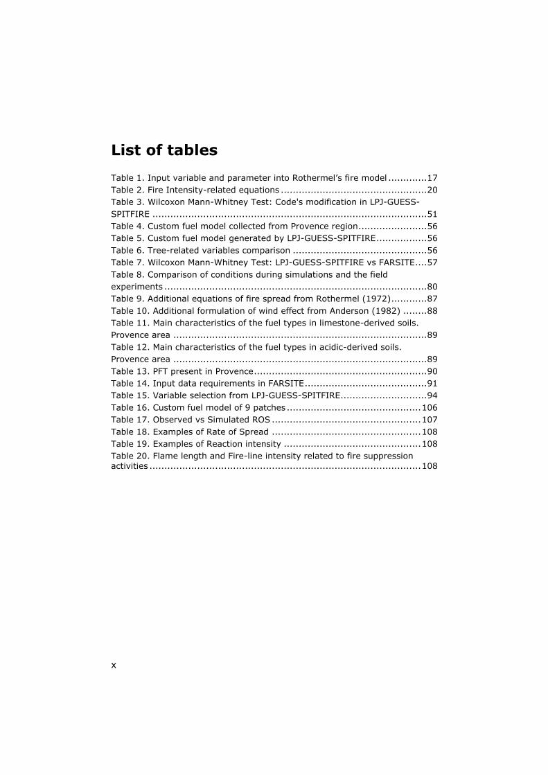
List of tables Table 1. Input variable and parameter into Rothermel’s fire model ............. 17
Table 2. Fire Intensity-related equations ................................................. 20
Table 3. Wilcoxon Mann-Whitney Test: Code's modification in LPJ-GUESS-
SPITFIRE ............................................................................................ 51
Table 4. Custom fuel model collected from Provence region ....................... 56
Table 5. Custom fuel model generated by LPJ-GUESS-SPITFIRE ................. 56
Table 6. Tree-related variables comparison ............................................. 56
Table 7. Wilcoxon Mann-Whitney Test: LPJ-GUESS-SPITFIRE vs FARSITE .... 57
Table 8. Comparison of conditions during simulations and the field
experiments ........................................................................................ 80
Table 9. Additional equations of fire spread from Rothermel (1972) ............ 87
Table 10. Additional formulation of wind effect from Anderson (1982) ........ 88
Table 11. Main characteristics of the fuel types in limestone-derived soils.
Provence area ..................................................................................... 89
Table 12. Main characteristics of the fuel types in acidic-derived soils.
Provence area ..................................................................................... 89
Table 13. PFT present in Provence .......................................................... 90
Table 14. Input data requirements in FARSITE ......................................... 91
Table 15. Variable selection from LPJ-GUESS-SPITFIRE ............................. 94
Table 16. Custom fuel model of 9 patches ............................................. 106
Table 17. Observed vs Simulated ROS .................................................. 107
Table 18. Examples of Rate of Spread .................................................. 108
Table 19. Examples of Reaction intensity .............................................. 108
Table 20. Flame length and Fire-line intensity related to fire suppression activities ........................................................................................... 108

xi
List of equations Equation 1. Rate of Spread (Frandsen 1971) ........................................... 18 Equation 2. Rate of Spread (Rothermel 1972) .......................................... 18 Equation 3. Reaction Intensity (Rothermel 1972) ..................................... 19 Equation 4. Byram’s fire line Intensity (Byram 1959) ................................ 20 Equation 5. Flame depth (Andrews 1986) ................................................ 20 Equation 6. Heat per area (Andrews 1986) .............................................. 20 Equation 7. Flame residence (Andrews 1986) .......................................... 20
Equation 8. Flame length (Andrews 1986) ............................................... 20

xii
Abbreviations
The models:
LPJ- Lund & Potsdam & Jena
DGVM- Dynamic Global Vegetation Model
GUESS- General Ecosystem Simulator
SPITFIRE- Spread and Intensity of Fire
FARSITE- Fire Area Simulator
The fire behaviour-related variables:
ROS- Rate of Spread
IR- Reaction of intensity
FLI-Fire line intensity
FML-Flame length
HPA-Heat per area
The institution:
IRSTEA- Institut national de recherche en sciences et
technologies pour l'environnement et l'agriculture

1
1. Introduction
Land biosphere plays a vital role on the global carbon cycle, the
climate system and it is an important part of global vegetation’s
shaping (Prentice et al. 2001). In the biosphere, complex
mechanisms and processes perform at multiple inter-related spatio-
temporal scales. These processes interact most of the time between
them all, allowing feedback loops effects without clear and visible
consequences. In System Earth everything is connected (Dopheide et
al. 2012). An example of such kind of processes are natural
disturbances. Even though disturbances impact over the system’s
balance, they are simultaneously an intrinsic part of the ecosystems,
which means that it is a factor needed for the preservation of many
cyclic natural structures (Prentice et al. 2007).
Fire is one of the primary global disturbance factors in all terrestrial
ecosystems (excluding the polar and desert biome), including soil and
litter, disrupting its structure and composition (Pyne et al. 1996). It
also has a large-scale relation with the climate conditions and has
effects on carbon storage or biochemical cycles (Thonicke et al.
2001). Annual global carbon emissions (from biomass burning) make
a substantial contribution into the tropospheric carbon budget,
estimated in a range from about 1.7 to 2.5 PgC (Thonicke et al.
2010). Since ignition, fuel composition and dryness are the main
control factors of fire at local level, both climate and vegetation
dynamic are closely interconnected with the fire performance and its
effects (Bowman et al. 2009).
The increasing number of evidences about a potential speed up of the
global warming (Houghton et al. 2001) has generated a demand for
tools that can predict the risks of dramatic environmental changes.
(Prentice et al. 2007). This request can be partly satisfied by
environmental modelling and it became an important research
pathway, facilitated at the same time by technological improvement.
Since the 70s, there was a need for a better understanding and
quantification of different control factors as well as interrelation
between processes, causes and consequences of wildfires within
Earth system dynamics (Bowman et al. 2009). Such kind of task can
be addressed by process-based models validated either through field
data and/or satellite imagery. A potential extrapolation of results into
speculative “what if…?” future scenarios provide modelling
approaches with an extra motivation.

Introduction
2
1.1 Problem statement
When modelling a fire behaviour, different approaches have been
attempted depending on the spatial scale: from methods concerning
fine spatial resolution, focusing on local and well-defined conditions,
to studies involving coarse resolution. The state-of-the-art of
worldwide terrestrial biosphere models, which represent vegetation
dynamics as well as biochemical process, are represented by Dynamic
global vegetation models (DGVMs) (Cramer et al. 2001; Smith et al.
2001; Thonicke et al. 2001; Sitch et al. 2003; Arora and Boer
2005; Prentice et al. 2007; Li et al. 2012). Fire modules have been
embedded in these models testing fire spread and intensity
simulations together with fire-vegetation interaction and post-fire
mortality (Thonicke et al. 2010), spatio-temporal fire regimes
(Venevsky et al. 2002; Lehsten et al. 2010), fire-climate feedbacks
(Archibald et al. 2010) as well as biomass burning emissions (Lehsten
et al. 2009; Thonicke et al. 2010).
Although the models’ performance has enhanced fire phenomena
characterization along the last decade, unavoidable limitations have
been detected by the simple fact that models are simplifications of
what occurs in reality. Glob-FIRM (Thonicke et al. 2001) allowed
fractional burnt performance in grid cell basis, depending only on the
length of the fire season and fuel loading. On the other hand it
neglects any characterization of ignition source as well as the wind’s
influence over the rate of spread. The model also disregards an
incomplete combustion of plants, i.e. assumes a constant fire-induced
mortality rate for each plant functional type (PFT). Reg-FIRM
(Venevsky et al. 2002) integrated a climatic fire danger, fire ignition
source and explicit model rate of spread. It does not measure any
trace gasses and aerosol emissions. Similar to Glob-FIRM, fire-
induced effects over the vegetation remain absent. MC-FIRE
embedded in MC1 DGVM (Lenihan et al. 1998) incorporated a novel
post-fire mortality computation according to Cohen and Deeming
(1985) even though unrealistically only allows one ignition per grid
cell per year. CTEM-FIRE (Arora and Boer 2005) presented a
simulation model of fire activity and novel biomass burning
emissions. Fire-induced consumption of biomass and plant mortality
is prescribed independent of fire intensity. Litter and litter moisture
were not included explicitly.
Due to the ongoing improvement of computer’s performance, a
further twist concerning modelling calculations became affordable,
significantly increasing the computational-complexity environments.
Proof of this progress is the fire module SPITFIRE, which has been

Chapter 1
3
embedded into LPJ-DVGM (Thonicke et al. 2010), into LPJ-GUESS
(Lehsten et al. 2009) and finally into LPX (Prentice et al. 2011). The
model performs computations in coarse spatial resolution, 0.5° grid.
It distinguishes different dead and live fuel classes, fuel loads as well
as moisture ratios. The basic physical properties and processes
determining fire spread and intensity were taken from Rothermel
(1972) applying some modifications. It also implements formulation
about fire-effect on vegetation as a function of structural plant
properties as well as trace gases and aerosol emissions (Thonicke et
al. 2010). LPJ-SPITFIRE framework presents at the same time a
number of limitations such as (1) does not take into account slope,
despite this being an important parameter concerning fire spread, (2)
some input variables are directly prescribed from literature (which in
certain conditions derivate in peculiar results), (3) overestimation of
burnt areas in some regions and underestimations in others (4) does
not characterize more than 1 day fire performance, (5) flaws in fuel
moisture calculations and therefore (6) unrealistic modelling of rate of
spread (most likely in grasses) . Improvements on the model have
been described by Pfeiffer and Kaplan (2012).
On the other hand, up-to-date modelling techniques at lower scale
follows a slightly different procedure (Albini 1976a; Albini 1979;
Andrews 1986; Scott and Reinhardt 2001; Finney 2004; Scott and
Burgan 2005). Although local fire behaviour models are based on the
same parameterization principles as those followed by fire modules
embedded in DVGM, the level of detail extensively changes. This kind
of models allows fire modelling at relative fine scale (i.e. local, 1 km
or even less). An explicit spatial component is typically included,
facilitating the interoperability with GIS software packages. It also
includes processes topography-dependent lateral fire spread which
deepens more into a realistic representation. Fire behaviour such as
crowning, torching and spotting could have been successfully
implemented. FARSITE (Fire Area Simulator), developed by USDA
Forest Service, is a fire growth simulator which has been widely
utilized as well as evaluated at different ecosystems all over the
world. It can spatially and temporally compute fire spread, intensity
or different post-frontal fire behaviours such as carbon biomass
emissions. The outputs are more reliable and accurate than the ones
from coarse scale.
Additionally to field measurements, Salis (2007) attempted the
validation of simulated rate of spread (ROS) in North Sardinia along
four different locations, each of them with different conditions. A
table enclosed in Annexe 7.12 reproduce the most important
characteristics reported, such as dominant species, plant height,
Introduction
4
temperatures or wind as well as the observed and the simulated ROS.
The author has simulated ROS up to 11 m/min under relative high
wind speed conditions. The results accurately match measured field
observations. Salis proposed two important interpretations from
these results: (1) as long as an accurate custom fuel model is
developed together with a precise wind’s dataset for a region with
specific conditions such as Mediterranean basin, then (2) FARSTE
allows very precise and accurate fire behaviour simulations
Embedding FARSITE into LPJ-GUESS for this purpose seems to be
suitable because: (1) LPJ-GUESS can simulate vegetation-related
inputs: (dynamic) fuel composition, fuel loading and fuel moisture (2)
the results from FARSITE can be approximated by a mathematical
model for predicting fire spread in equations, (3) it allows the same
assumption about elliptical spread shape and (4) both models follow
the Huygen’s principle involved in fire growth computation.
1.2 Aim and objectives
To simulate the effect of fire on the dynamic vegetation at a fine
scale, I will attempt the assessment of a potential fire meta-model
running into the modular framework of Lund-Potsdam-Jena General
Ecosystem Simulator (LPJ-GUESS) (Smith et al. 2001).The main aim
of this Master thesis is to evaluate the potentials from embedding
vegetation dynamic (LPJ-GUESS-SPITFIRE) into a spatial-explicit fire
behaviour model (FARSITE): LPJ-GUESS-FARSITE. The research took
a local perspective supported by field data in order to establish a
robust starting point. Understanding how fire performs in a local scale
would most likely allow fire behaviour upscaling in future, before
focussing on coarse resolution directly. The case study area is centred
on the Maures massif, a characteristic landscape located in Provence
(France).
Since flaws in performance and lacks in relevant input variables
directly influencing fire behaviour were reported, the hypothesis for
this thesis is that both FARSITE and LPJ-GUESS-FARSITE outputs are
expected to be more realistic than LPJ-GUESS-SPITFIRE output. The
null hypothesis establishes no significant difference between LPJ-
GUESS-SPITFIRE, FARSITE and LPJ-GUESS-FARSITE outputs.
Chapter 1
5
In order to do so, the main research questions addressed in this
research are:
RQ 1 Does LPJ-GUESS-SPITFIRE represent the actual vegetation
from Provence? Does the fire return interval influence
ecosystem succession in a realistic manner (in comparison
to field measurements) in the study area?
RQ 2 Does LPJ-GUESS-SPITFIRE get similar fuel- and tree-
related estimations from vegetation in comparison with
data collected on the field along the study area?
RQ 3 Does the existing LPJ-GUESS-SPITFIRE model represent
realistic and accurate fire spread as well as fire intensity?
RQ 4 Does LPJ-GUESS-FARSITE represent realistic and accurate
rate of spread as well as fire intensity?
RQ 5 Does LPJ-GUESS-FARSITE perform better fire behaviour
than LPJ-GUESS-SPITFIRE? Can the estimations be
improved?
In order to answer these questions, the following steps will be
required:
Assessing variable selection and its range at which FARSITE
needs to be run.
Assessing initializers parameters at which LPJ-GUESS-
SPITFIRE needs to be run.
LPJ-GUESS-SPITFIRE’s code implementation.
Simulation of the typical LPJ-GUESS conditions for the cases
study area.
Running FARSITE for the range of conditions in LPJ-GUESS-
SPITFIRE.
Comparison of the results from LPJ-GUESS-FARSITE with the
results from LPJ-GUESS-SPITFIRE.
Evaluation of both FARSITE and LPJ-GUESS-SPITFIRE
estimations for a number of sample fires.
In the first chapter some background information about wildfires,
control factors, characteristic fire behaviour, fire recurrence and its
relationship with the vegetation, description of burnable fuel and
basic modelling parameterization are given. In chapter 3, the study
area and the models used are presented, followed by the
methodology used in this thesis. The results are presented in chapter
4 and discussed in the subsequent chapter 5. In the final chapter, a
conclusion for the main research questions are given. A set of
annexes are enclosed supporting concepts, ideas as well as adding
extra information.

Introduction
6
7
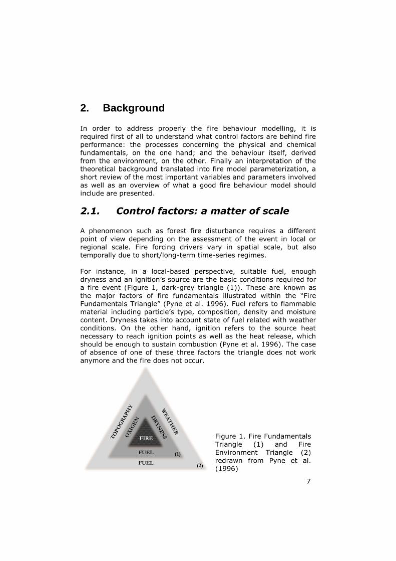
Figure 1. Fire Fundamentals
Triangle (1) and Fire
Environment Triangle (2)
redrawn from Pyne et al.
(1996)
2. Background
In order to address properly the fire behaviour modelling, it is
required first of all to understand what control factors are behind fire
performance: the processes concerning the physical and chemical
fundamentals, on the one hand; and the behaviour itself, derived
from the environment, on the other. Finally an interpretation of the
theoretical background translated into fire model parameterization, a
short review of the most important variables and parameters involved
as well as an overview of what a good fire behaviour model should
include are presented.
2.1. Control factors: a matter of scale
A phenomenon such as forest fire disturbance requires a different
point of view depending on the assessment of the event in local or
regional scale. Fire forcing drivers vary in spatial scale, but also
temporally due to short/long-term time-series regimes.
For instance, in a local-based perspective, suitable fuel, enough
dryness and an ignition’s source are the basic conditions required for
a fire event (Figure 1, dark-grey triangle (1)). These are known as
the major factors of fire fundamentals illustrated within the “Fire
Fundamentals Triangle” (Pyne et al. 1996). Fuel refers to flammable
material including particle’s type, composition, density and moisture
content. Dryness takes into account state of fuel related with weather
conditions. On the other hand, ignition refers to the source heat
necessary to reach ignition points as well as the heat release, which
should be enough to sustain combustion (Pyne et al. 1996). The case
of absence of one of these three factors the triangle does not work
anymore and the fire does not occur.
FIRE
FUEL
FIRE
FUEL
(1)
(2)
Local scale
Landscape scale
Background
8
When up-scaling from local perception into landscape-based level, the
fire behaviour is defined by weather, topography and fuel (Figure 1,
light-grey triangle (2)). The three of them are the main drivers
behind the “Fire Environment Triangle” (Pyne et al. 1996). The
interaction of these factors and with the fire itself will define the fire
behaviour. Topography refers directly to slope, aspect and elevation
although it also can indirectly influence fuel and weather
characteristics. Fuel is a critical factor within fire behaviour and it
depends on, among other things, fuel size, fuel dead/live composition
and moisture (Fuel models are reviewed more in detail at point 2.4).
Weather variables such as temperature, precipitation, relative
humidity and wind (this latter has great impact over fire spread)
influence fire ignition as well as the fuel state.
In order to understand properly the “rich picture” about main drivers
involving global-based wildfires, an extra triangle is required. The
extension would depend on vegetation, climate and land use
(Bowman et al. 2009), being the latter triangle beyond the scope of
this research. This framework helps to put cause-effect feedbacks
between the vegetation dynamics’ state, influence of environmental
conditions and wildfires’ impacts estimation along the system in
context.
2.2. Fire behaviour
Wildfire dynamics go through several stages ranging from pre-
ignition, ignition, combustion and extinction. First of all an ignition is
needed in the form of heat supply for fuel available in the
surroundings. Dehydration, pyrolysis and release of gases follow the
process. If the gases emission from fuel are suitable, it ignites a
flame and the fire has the possibility to spread to a different location
(Rothermel 1972). Combustion occurs when fire spreads either in
form of flaming or smouldering, releasing heat in form of exothermic
reaction. If not enough heat or source of heat is longer available, the
extinction of the fire occurs.
Wildfires can be started by natural or anthropogenic events. Lightning
strikes are the main natural ignition sources. Land (field)
management activities such as agriculture or forestry, discarded
cigarettes or high-power-lines are examples of man-made sources.
Spontaneous ignition has also been observed as consequence of
internal heating in hay, chip and sawdust’s pile (Pyne et al. 1996;
Johnson and Miyanishi 2001). The stochastic nature of fire
disturbance significantly increases the difficulty of fire behaviour
modelling (Prentice et al. 2007).

Chapter 2
9
In general there is a single source point from where the fire spreads.
Two different states representing fire growth after the ignition
episode can be characterized: acceleration (also called build-up) and
quasi-steady-state time (Chandler et al. 1983; Pyne et al. 1996). The
acceleration time represents the period of time from ignition until fire
reaches the equilibrium state. Reached this stage, fire has a constant
forward speed, i.e. steady rate of spread (Rothermel 1972). A fire
acceleration model for open canopy by the Canadian Forest Fire
Prediction System is shown in Figure 2.
Figure 2. Fire model from FCFDG (1992)
A fire growing event from a point of ignition to each point of the fire
front will evolve an elliptic shape of spread assuming moderate wind
effect as well as homogenous fuel and weather conditions (Weber
2001). The elliptical representation, widely used in literature
(Rothermel 1972; Andrews 1986; FCFDG 1992; Finney 2004;
Thonicke et al. 2010; Pfeiffer and Kaplan 2012), can be used to
characterize the shape of fire from the point source in such a way
that: (1) higher length-to-width ratio in increasing slopes and in the
direction of wind (i.e. faster fire spread), (2) front-back-flank
represent respectively the fastest, slowest and intermediate
spreading part of the fire and (3) the more homogenous conditions
(for instance fuel, wind or slope) the less irregular elliptical shape.
These three behaviour patterns are represented in Figure 3.

Background
10
Figure 3. Elliptical rate of spread´s shape. Based on FCFDG 1992 and
FARSITE’s technical documents
Three different types of fire can be well-defined conditional upon
what kind of fuel is available for combustion: ground, surface and
crown fires. Ground fires typically burn material underneath the
superficial layer. Duff, which has high organic carbon content,
exemplifies a kind of peat land liable to post-frontal combustion.
Surface fires perform at the superficial level burning grasses, shrubs,
dead branches, forest needles or leaf-sapwood-heartwood litter.
Classical fire modelling was first performed experimentally in the 70s
based on this fire class. Crown fires have typically got up from the
ground and burnt either tree or/and shrubs canopies. Crown fires can
derive into extreme fire behaviour such as torching or spotting
increasing fire intensity and the impacts carried out. Torching refers
to the sudden canopy ignition from surface due to the intensity,
whereas those new fire spots are originated beyond fire-line as
consequence of firebrands fliers caused by spotting (Chandler et al.
1983; Pyne et al. 1996).
In order to acquire a meaningful understanding about fire behaviour,
three concepts need to be introduced. The desire to address
suppression and management of natural resources during fire events
as well as assessment of fire effect over plant communities (Johnson
and Miyanishi 2001) established fire characterization of rate of spread
(ROS) together with fire intensity and post-frontal combustion (i.e.
burning emissions).

Chapter 2
11
ROS refers to the speed (average m/min) at which the fastest section
of the fire perimeter, also called fire-line, spreads into unburnt fuels,
following the perpendicular direction to the perimeter. Fluctuating
conditions can easily alter the spread rate. Wind and slope are
sensitive variables affecting ROS behaviour and it depends on
direction and magnitude. Fires tend to fast-spread at up-slopes as
well as in the wind direction although it is also possible downhill due
to combined wind effect. Likewise fuel characteristic is a critical
variable involving fire spread. For example fine dead material such as
grass, leaf or needle litter burns faster than heavy trunks or duff,
which can remain smouldering afterwards the fire-line passed (Pyne
et al. 1996).
The fire intensity, following the United States fire behaviour
prediction system, can be measured by flame length, fire-line
intensity, reaction intensity and heat per unit area (Andrews 1986).
Fire-line intensity, also called Byram’s intensity (FLI), is the heat
released per unit of time per front-rear distance of the flaming zone
(kW/m), called flame depth (Byram 1959). Reaction intensity (IR)
refers to heat released per area per time unit in the flaming zone
(kW/m2). Heat per unit area (HPA) account for the heat emitted per
area during whole flaming event (kJ/m2). Flame length (FML) is the
distance between the average flame front to the middle of the
flaming zone (m) (Pyne et al. 1996; Alexander and Cruz 2012).
Typical examples of fire intensity together with rate of spread
prescribed by Albini F.A (unpublished training notes reported in Pyne
et al. (1996)) are enclosed in the annexe 7.4. The units were
conveniently transformed from English to Metric units. In a like
manner, fire behaviour has been characterized through laboratory
and field measurements (Cheney and Gould 1995; Morandini et al.
2005; Morandini et al. 2006; Santoni et al. 2006; Silvani and
Morandini 2009; Curt et al. 2010; Curt et al. 2011; Ganteaume et al.
2011; Silvani et al. 2012). This valuable information can be used as a
guideline for fire model’s validation.
Even though the fire front has long passed, active processes still can
remain active. If soils with high organic composition are available,
potential smouldering combustion could occur for days, months or
even years. Decomposed plants with low concentration of cellulose
and higher concentration in lignin favour the process. Likewise post-
frontal combustion burns woody surface fuels and litter. Fuel closely
packed such as woody debris are more likely to smoulder rather than
fine litter (Pyne et al. 1996). Fuel composition in these conditions
tends to release great flux from burning emissions. As rule of thumb:
Background
12
the dryer the fuel and the more oxygen is available, the more CO2 is
produced; and the wetter and less oxygen is available, the higher the
ratio of trace gases like methane, CO or VOCs is (Lehsten 2013).
Lastly, the feedbacks loop prediction between fire and climate
became a crucial matter (Rothermel 1991; Lehsten et al. 2009;
Thonicke et al. 2010). Understanding how relevant the fire
contribution into the system is, allows speculations about what could
be derived in future scenarios.
2.3. Fire recurrence
According to Gill (1979), the fire regime is characterized by the
association of the fire spatial pattern as well as the fire intensity, the
fire seasonality and the fire recurrence, all of them befalling an
specific target area. The fire recurrence itself represents the temporal
quantification of how often the area is affected by the impact of a
fire. At the same time, fire recurrence can be divided into both (1)
fire frequency, standing for the number of fire events taking place
within a specific area during a specific period of time (Eugenio et al.
2006); and (2) fire return interval, which represents the period of
time in between two successive fires (Schaffhauser et al. 2011).
The fire return interval plays an important role over the response
experienced by plants and ecosystems due to fire disturbance. As
said by Malamud and Turcotte (1999), wildfires and vegetation are
most likely to establish positive feedback loops in between of them.
For instance, fire can affect the structure and composition of the
vegetation, which, at the same time, affects behaviour of future
disturbance events. The plant regeneration capacity, also called post-
fire resilience, establishes two well defined kind of plant adaptation
facing wildfires: resprouters species (characteristic from long fire
recurrence) versus seeders species (typically found within large fire
return intervals) (Pausas 1999; Acácio et al. 2009; Curt et al. 2009;
Schaffhauser et al. 2012b).
2.4. Fuel
According to Paysen et al. (2000) available fuel refers to the amount
of either dead or living biomass that burns under a given set of
conditions. Fire dynamics is dependent on the fuel availability whilst
fuel moisture is strongly dependent on environmental conditions.
Once fuel is ignited, litter fuel can expand both in horizontal and
vertical direction (Plucinski and Anderson 2008). As fire fundamentals

Chapter 2
13
and environmental triangles illustrated at point 2.1, the fuel
component is present in both local and landscape-based scenario,
playing a crucial role. Fuels affects either how easily a fire ignites, its
rate of spread, its intensity or the burning emissions (Rothermel
1972; Andrews 1986; Scott and Burgan 2005).
Following Pyne et al. (1996) fuels can be classified based on its type,
its state or its size (diameter). Fuel type describes the fuel itself and
the physical properties related to fire. Fuel state takes into account
environmental conditions such as the moisture content.
2.4.1. Fuels characteristics
Quantity, size and shape, compactness and arrangement (Chandler et
al. 1983; Pyne et al. 1996) are the most common physical properties
in regards to fuel. Fuel loading is the amount of both aboveground
dead and living fuel to be found. It is quantified by measurements of
fuel’s oven-dry weight per area (T/ha). Measuring oven-dry weight
allows the independent categorization of moisture’s parameter. Size
gives an idea about how fine or coarse the fuel’s target is and usually
is defined by surface-area-to-volume (SAV) ratio. The higher the
SAV ratio, the finer the fuel is, hence the easier to ignite. It relates
directly to ignition time and ROS. Compactness relates to the space in
between fuel particles. Nevertheless fuel bulk density is the most
common way of representing the fuel porosity, i.e. fuel weight divided
by volume. It directly affects ignition time as well as how combustion
performs. Finally, arrangement establishes a criterion for fuel
orientation (horizontal vs vertical) together with its spatial
distribution, level of mixture and live-to-dead ratio. In Figure 4
different fuel groups are oriented in two basic directions depending on
relation fuel depth-fuel load: vertically, as in grasses and shrubs, and
horizontally, as in timber, litter, and slash (Anderson 1982).
Barrows (1951) categorized fuel into ground, surface and crown
classes according to vertical strata. The ground material is mostly
composed by roots and duff. Superficial fuel includes small trees and
shrubs, forest litter and fallen wood, grasses and litter formed by
fallen leaves, twigs, needles, steams and bark. Crown fuel refers
specifically to large shrubs and canopy (stand height) trees. A
combination of different layers are defined as fuel complexes (Scott
and Burgan 2005). The classification proposed establishes an
inflexion point for the separation of surface fire spread computation

Background
14
Figure 4. Vertical vs horizontal orientation based on fuel
depth-fuel load relation according to Anderson (1982).
(Rothermel 1972) and crown based phenomena (Scott and Reinhardt
2001).
2.4.2. Fuel moisture
Fuel moisture, dependent on environmental conditions, strongly
regulates both dead and living material available for combustion.
Water is evaporated before the fuel could be heated up to the
temperature required for ignition. For this reason a low degree of
humidity can be derived into greater facility for pre-heating and
ignition, acceleration of combustion and higher fire spread and
intensity. Hence fuel moisture affects important aspects of fire
behaviour such as ROS, intensity, smoke production, fuel
consumption and plant mortality (Pyne et al. 1996).
According to Fujioka et al. (2008) fuel moisture is derived as “the
mass of water present in the fuel”. It is generally expressed as
fraction of water mass (i.e. initial fuel mass minus dry mass) divided
by the oven-dry fuel mass. The percentages can widely vary

Chapter 2
15
depending on whether dead fuel (from 1 or 2% in deserts to 30% due
to fibre saturation or even up to 300% on decayed woody) or live fuel
(ranging from 50% up to 1000% because of duff) are present.
Dead fuel moisture is influenced mainly by environmental factors
such air temperature, relative (air) humidity, solar radiation and
rainfall. These are dependent on local topographic and site factors
like elevation, slope, aspect, canopy cover, fuel composition and fuel
size (Finney 2004). On the other hand, as noted by Rothermel
(1983), live fuel moisture is a function of the physiological processes
occurred in the plants. Moisture content is influenced by factors such
us seasonality, precipitations, temperature or the plant species
themselves. Dead fuel size can be classified based on the response to
environmental changes by moving its moisture to a new equilibrium.
Fuel diameters have been matched according to their “time lag”.
Time lag is defined as the time period required for a dead fuel to
respond within 63.2% of the new equilibrium moisture content
(Missoula Fire Science Laboratory 2010). This means that thinner
diameters have lower time lags, hence a faster response to changes
in the environmental conditions than thicker fuel sizes. This can be
observed in Figure 5. Time lag categories used for fire behaviour were
specified as 1hr (leaves and twigs), 10hr (small branches), 100hr
(large branches) and 1000hr (boles and trunks).At the same time
Figure 5. Graph of fuel moisture content over 3 time-lags of dead fuel
in FARSITE
these categories represent the size classes: 0-.635cm, 0.635-2.54cm,
2.54-7.62cm and 7.62-20.32cm respectively (Andrews 1986). Even
though it is an oversimplification, this terminology is still used (Finney
2004; Thonicke et al. 2010; Pfeiffer and Kaplan 2012).
Background
16
2.5. Basic parameterization in fire modelling
Generally speaking, there are three different methods which can
predict fire behaviour. These are empirical, statistical and theoretical
(Chandler et al. 1983). Empirical models require large fires dataset
where all parameters except one are constant in order to evaluate the
effect over ROS and IR. The main disadvantage of this approach is
the interaction effect between variables, as it has a tendency to be
overlooked. Statistical methods are supported by variants of classical
multiple-regressions models. Although it provides confidence limits
about the ROS prediction, either non-linear relation between variables
nor compulsory entire calculation when new data are included make
this methodology challenging.
The theoretical models are based on physical and thermo-dynamical
principles. The advantage of these models are the use of well-known
and verified relationships allowing up-scaling, hence the validation
process is easier and dataset requirements are reduced in comparison
to other approaches (Chandler et al. 1983). This thesis presents work
related with the theoretical (process-based) model.
2.4.3. Fuels models
Mathematical fire behaviour models such as Rothermel (1972) require
a specific and detailed fuel description. Since the fire model is a set of
equations, the fuel model is characterised by a specific set of fuel-bed
inputs fitting into the parameterization. It is essential for ROS, fire
intensity and burning emission computations (Pyne et al. 1996). Fuel
models are tools which simply help the user to realistically estimate
fire behaviour (Anderson 1982; Scott and Burgan 2005). In Behave
and FARSITE there are two different kinds of fuel models:
Static fuel models: aiming at fire spread prediction.
Dynamic fuel models: pointing at fire danger rating system
(NFDRS) but beyond the scope of the present study.
Although fuel models try to reduce the complexity within fire
modelling, it is challenging to adequately characterize heterogeneous
complexes (reviewed at point 2.3.1), where large differences in
physical properties such as surface-to-volume ratio or fuel height can
diverge greatly.
Chapter 2
17
One of the first attempts at establishing a fire behaviour fuel model
was Rothermel (1972) over his fire spread prediction model. He took
into account 11 different fuel types. The fuel models were defined by
fuel loading by size class (Tons/Ha), fuel depth (m) and fuel particle
size (fine, medium, large). Particle density, heat content, total /
effective mineral content and moisture of extinction were constant-
defined. Albini (1976a) improved those 11 fuel models adding two
more (11+2) and reclassified both within 4 groups: grass- , shrub- ,
timber- and slash-dominated. At the same time a specific moisture of
extinction, referring to moisture content at which fire will not spread
(Rothermel 1972), for each fuel type was defined. The previous set of
constants remain without changes. BEHAVE (U.S.) fire behaviour
prediction developed by Anderson et al. (1982) defined fuel models
by vegetation types with specific heat content as well as specific
packing ratios for each fuel. FARSITE (Finney 2004) allowed dead/live
fuel differentiation in order to improve the accuracy of the
computations. Scott and Burgan (2005) refined the whole fuel model
developed until the date implementing up to 40 standard fire
behaviour fuel models. The required fuel input variable and
parameter selection for Rothermel’s fire model is presented below,
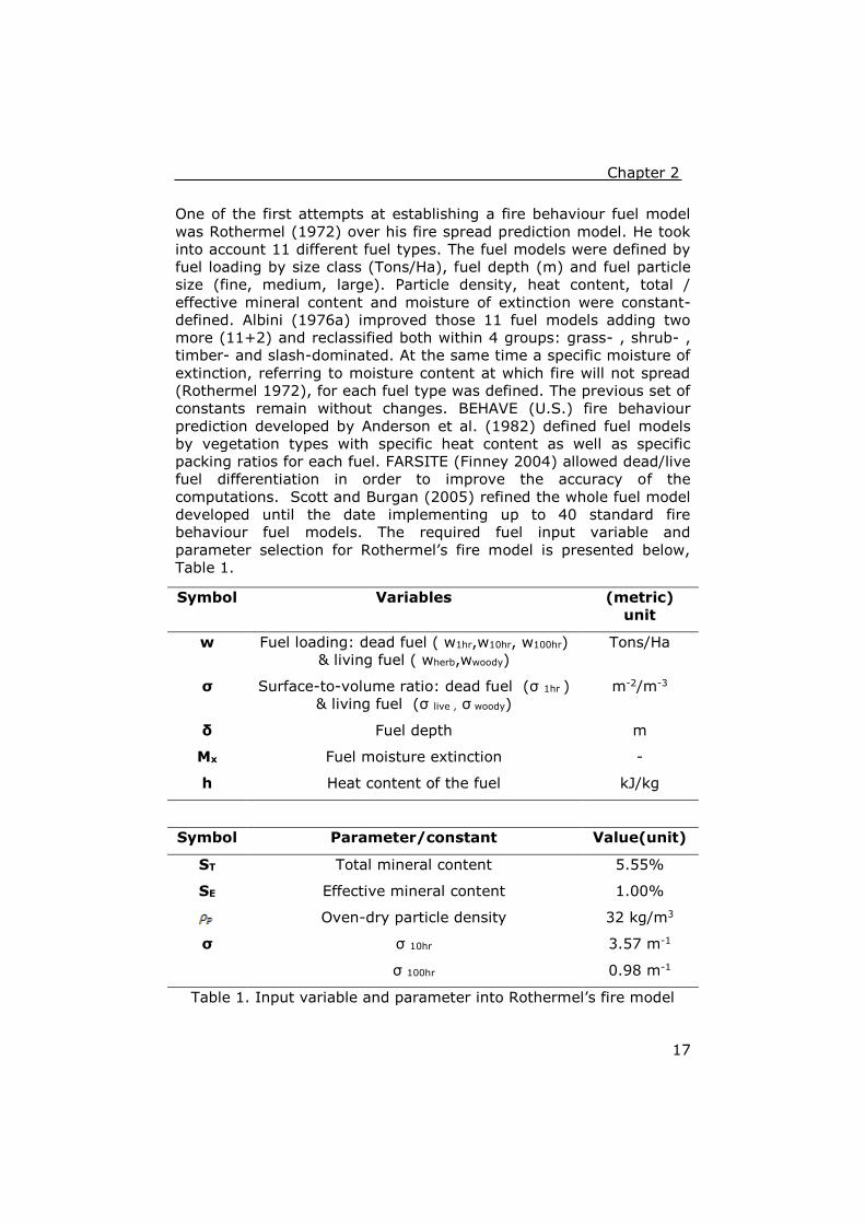
Table 1.
Table 1. Input variable and parameter into Rothermel’s fire model
Symbol Variables (metric)
unit
w Fuel loading: dead fuel ( w1hr,w10hr, w100hr)
& living fuel ( wherb,wwoody)
Tons/Ha
σ Surface-to-volume ratio: dead fuel (σ 1hr )
& living fuel (σ live , σ woody)
m-2/m-3
δ Fuel depth m
Mx Fuel moisture extinction -
h Heat content of the fuel kJ/kg
Symbol Parameter/constant Value(unit)
ST Total mineral content 5.55%
SE Effective mineral content 1.00%
Oven-dry particle density 32 kg/m3
σ
σ 10hr 3.57 m-1
σ 100hr 0.98 m-1

Background
18
2.4.4. Rate of spread
First attempts concerning mathematical models, making quantitative
estimations of ROS and IR, were performed in the early 70s. Authors
have realised that a correct prediction of ROS is given when the fire is
being driven by flame radiation, i.e. heat fluxes and required heats of
ignition. When fire reaches the called “quasi-steady state” (point 2.2)
the ROS is then a ratio between the heat flux received from the fire
and the heat needed for a latent fuel to be ignited (Rothermel 1972).
Frandsen (1971), applying the conservation of energy principle, has
proposed the following theoretical relation:
Where:
R = quasi-steady rate of spread.
Ixig = horizontal heat flux absorbed by a unit volume of fuel at
the time of ignition.
ρbe = effective bulk density (amount of fuel per unit volume of
the fuel bed).
Qig = heat of pre-ignition (the heat required to bring a unit
weight of fuel to ignition).
= the gradient of the vertical intensity evaluated at a
plane
zc = constant depth of fuel bed.
The horizontal and vertical coordinates are x and z,
respectively.
At that time it was not possible to find an analytical solution due to
the existence of certain unknown parameters. Rothermel (1972)
introduced the experimental and analytical formulation obtained in
the laboratory (cited formulation is included in Annexe 7.1). The
result given is:
This expression about ROS has two relevant signs of identity. Firstly,
since all parameters except mineral content and moisture of
extinction are measurable in the field, these equations were and still
are currently embedded in many fire behaviour models applied
worldwide (Rothermel 1972; Chandler et al. 1983). The other
(2)
(2
)
(1)
(1
)

Chapter 2
19
distinguishing features allow the assumption of elliptical spread shape
in order to develop an algorithm aiming at fire growth computation.
There is a direct dependence between elliptical fire shape and the
rate of spread behind Rothermel’s formulation and it is because it
just takes into account the front part of the fire simulation (Rothermel
1972). Minor formulation adjustments have been done by Albini
(1976a) afterwards.
Anderson et al. (1982) describes the elliptic spread’s shape
mathematically by parametric equation based on different scenarios,
firstly with no wind effect and secondly under constant wind
(parameterization included at Annexe 7.2 point 1.). The authors come
up with a modification of Huygen’s principle to model growing fire
spread in non-uniform conditions. The principle can be imagined as a
fire propagation over a finite time interval using points which define
the fire front. At the same time independent ignition sources of small
elliptical wavelets can be settled in there. These fires create an
envelope around the original perimeter, where the outer edge
represents the new fire front (Annexe 7.2 point 2.). This process has
been referred to as Huygens' principle (Anderson et al. 1982). This
approach allowed computer implementation of forest fire modelling in
many models.
Research related to computation of the rate of spread is mainly based
on Rothermel’s equations. Nevertheless it only takes into account the
front part of the fire simulation. Limitation such as spread of fire by
firebrand or crown fires were not included subtracting reliability and
accuracy to the estimations. Further implementations of surface fire
behaviour have introduced sub models in order to implement the
overall calculations. The inclusion of crown fire behaviour instead of
just superficial spread (Wagner 1977; Rothermel 1991; Scott and
Reinhardt 2001; Finney 2004), the creation of new fires generated
by spotting effect (Albini 1979) and post-frontal combustion (Finney
et al. 2003) allow much more realistic estimations and a better
understanding about how fire behaviour performs.
2.4.5. Fire intensity
Reaction intensity of a surface fire refers to thermal energy
production (i.e. rate of released energy per unit area) at the flaming
front. It was defined by Rothermel (1972) and subsequently re-
adapted by Wilson (1980):
(3)

Background
20
Where:
IR = Reaction intensity (kW/m2)
Г´ = Optimum reaction velocity (min -1)
wn= Net fuel load (fuel after substation of its mineral content
(kg/m2
h = Heat content of the fuel (kJ/Kg)
ηM= Moisture damping coefficient (from 0 to 1)
ηS= Mineral damping coefficient (from 0 to 1)
2.4.6. Byram’s fire-line intensity, flame length
and heat per area
The mathematical relation among IR, HPA and FML described by
Andrews (1986) (conveniently adapted to SI units) together with FLI
formulation prescribed by Byram (1959) are summarized in Table 2:
Table 2. Fire Intensity-related equations Reaction of intensity was taken directly from Rothermel (1972). Heat
per unit area is obtained from the multiplication of Rothermel’s
reaction intensity and Anderson’s residence time (Anderson 1969),
being the latter a function of the diameter of the fuel, directly related
to time lag (point 2.3.2). Fire-line intensity, also called Byram’s
intensity (Byram 1959) can be derived from three different
combinations of Rothermel’s model variables. It is considered one of
the most useful fire intensity’s measures (Chandler et al. 1983).
Flame length is directly related to fire-line intensity.

Chapter 2
21
2.5. What should a fire model embedded in a DGVM consider?
Coupling a fire model into a DGVM allows the simulation of inter-
related processes between the vegetation dynamics-climate-fire
behaviour predictions as well as the understanding of how feedback
loops affect the overall balance of the system. This task is challenging
since there are many multi-directional processes working at the same
time and because they are affected by the performance of several
parameters simultaneously. The delineation of clear and precise
components of conceptual framework and its boundaries are needed
in order to properly address fire modelling within dynamic global
vegetation models.
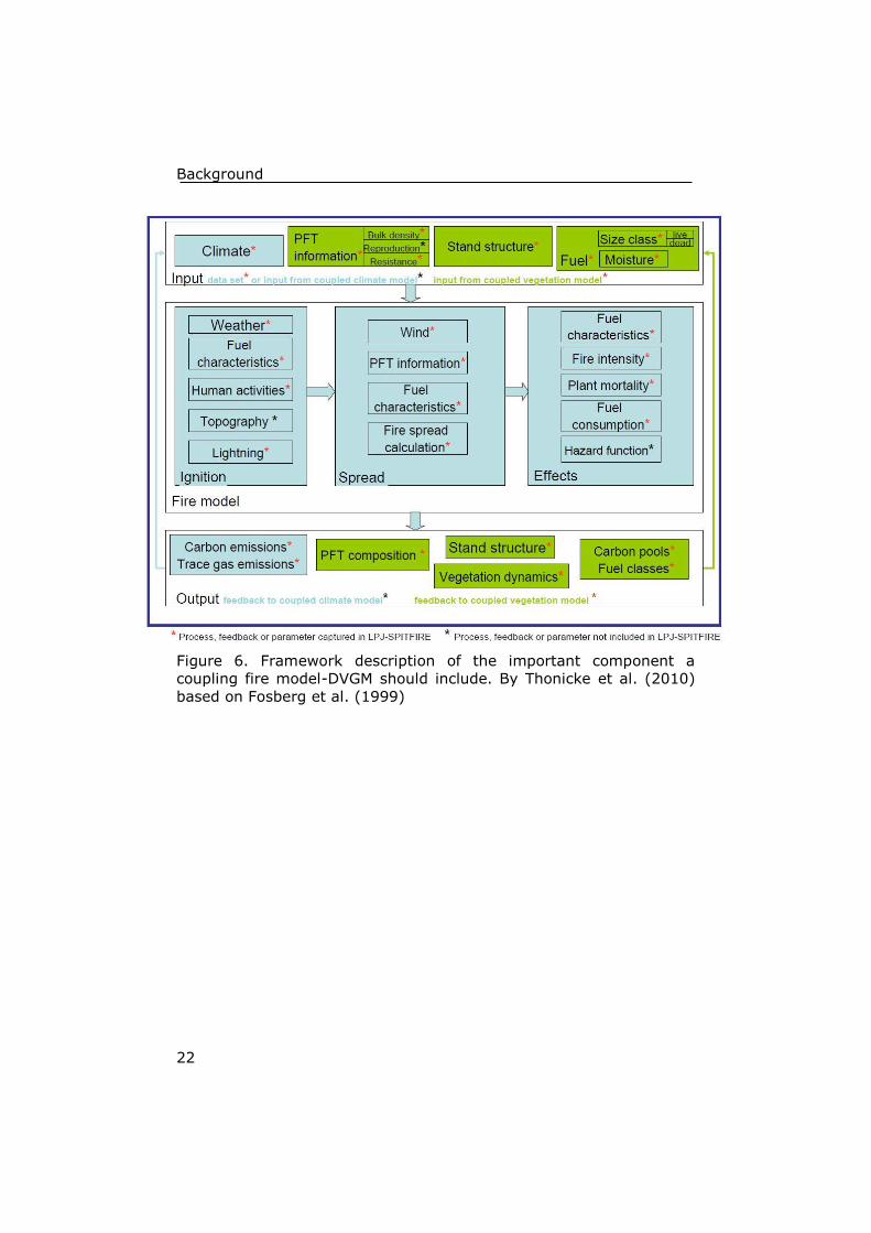
Fosberg et al. (1999) suggested a model framework with climate,
fuel’s load-size-moisture, plant functional types (PFT) composition
and stand structure as input data for the fire module. The fire
behaviour unit can be divided into different subsections based on the
processes involved, represented at Figure 6.
Weather, fuel, ignition source (natural and human based) and
topography parameters influence how fire ignites. On the basis of
these, ROS (more or less complex depending if spotting or crowing
calculations are included) performs as a consequence of wind, dead-
living fuel and the physics behind fire spread computation. Given a
specific ignition and spread, but also depending on fuel characteristic,
the effects allow quantification of fire intensity, fuel weight loss as
well as plant damage and mortality. The two latter directly affect
biomass burning emissions. Carbon emission, remaining PFT, stand
structure or vegetation dynamics are potential output data prescribed
by Fosberg et al. (1999) and plausible research target for feedback
loop assessment linking either fire, vegetation and/or climate.
Background
22
Figure 6. Framework description of the important component a
coupling fire model-DVGM should include. By Thonicke et al. (2010)
based on Fosberg et al. (1999)

23
3. Methodology
In order to assess the potential embedment of a dynamic vegetation
model (LPJ-GUESS) into a spatial-explicit fire behaviour model
(FARSITE), certain questions need to be answered following the
methodology presented in this chapter. A brief description of the
study area, followed by a sketch of the main model’s characteristics is
presented here. The method continues by: (1) assessing variable
selection at which FARSITE needs to be run, (2) assessing initializers
parameters at which LPJ-GUESS-SPITFIRE needs to be run, (3)
implementing the source code in LPJ-GUESS-SPITFIRE, (4) simulating
the typical LPJ-GUESS conditions within the case study area, (5)
running FARSITE for the range of conditions in LPJ-GUESS-SPITFIRE
and (6) comparing of the results from LPJ-GUESS-FARSITE with the
results from LPJ-GUESS-SPITFIRE.
3.1. Study area
The Provence region is located in the south-eastern part of France
(Aix-en-Provence 43°22N 05°27E). France is considered one of the
five southern member states in the EU that is most affected by wild-
fires (JRC-EFFIS 2012) since 2005’s annual report. For instance, in
2012 the annual burned area on average was counted on 8.600 ha
whereas 26.383 ha were affected by fires from 1980 to 2001. Fire, a
significant disturbance factor in Provence’s region, plays an essential
role within the vegetation dynamics shaping the structure and
composition of the landscape (Pausas 1999; Curt et al. 2011;
Schaffhauser et al. 2011).
A widespread range of Mediterranean type fire-prone ecosystems
(MTEs) covers this region (Curt et al. 2010). The study area is mostly
based on shrublands, forest and grassland. Afforestation of conifer
species, abandonment of agricultural land facilitating the shrubland’s
expansion as well as population’s increase constitute the main drivers
behind fire risk (Moreira et al. 2011; Curt et al. 2013). In this region
two key landscapes, based on soil substrate, were classified by
Quézel and Médail (2003). As a result of this categorization, (Curt et
al. 2010) described the relation of soils with regards to the presence
of dominant vegetation. For instance: (1) limestone substratum is
characterized by Quercus coccifera (shrub), Quercus Ilex, Quercus
pubescens and Pinus halapensis (both forest) (Ganteaume et al.

Methodology
24
Figure 7. Aix-en-Provene 43°22N 05°27E
2011), whereas (2) siliceous/acidic substrata is dominated by Erica-
Cistus spp (shrub) and Quercus Suber (forest)(Curt et al. 2009). A
table with further explanation on the main characteristics of the fuel
types (Curt et al. 2013) is enclosed in Annexe 7.3.
The siliceous area, belonging to the so-called Maures massif (shown
in Figure 7, within the red boundary), is influenced by Mediterranean
climate. Following the climatic indices given by Sitch et al. (2003),
Maures massif fits in the bioclimatic zone 8. This represents a drought
tolerance >0.4, temperature of coldest month >1.5ºC and growing
degree days (5ºC)>2500. The mean annual rainfall approaches the
550 mm in lowland but ca. 1000 mm/year on the massif ridges,
whilst the mean annual temperatures are 15.9ºC. These conditions,
together with high inter-annual and seasonal variability plus strong
winds and tendency to droughts, make the Provence region a fire-
prone environment (Curt et al. 2013).
Chapter 3
25
3.2. Fire behaviour models
3.2.1. LPJ-GUESS-SPITFIRE
The structure, composition and dynamics of terrestrial ecosystems
can be modelled with LPJ (Lund-Potsdam-Jena) framework at
different scales, ranging from landscape up to worldwide scale. The
representation of the vegetation in LPJ is characterized by Plant
Functional Types (PFTs). PFT refers to a set of one up to large
number of species with similar characteristics such as growth form
(grass, shrub or tree), leaf form (broad or needle leaf), leaf
phenology (evergreen, summer-green or rain-green), leaf physiology
(C3 or C4 grasses) and bioclimatic limitations (drought tolerance,
temperature of coldest month or growing degree days on based
5ºC)(Fosberg et al. 1999; Smith et al. 2001; Sitch et al. 2003). In
LPJ version 2008 there are 20 PFT, 18 woody-based species and 2
types of grasses. An overview of PFT present in the study area as well
as its taxa characterization and description is included in the Annexe
7.4.
Fire was the only natural disturbance computed in the very first
version of LPJ (Sitch et al. 2003). However, this first formulation was
rather simple and further development was required due to the
significant limitations concerning fire performance. Advances were
achieved by Thonicke et al. (2010) when coupling SPITFIRE (Spread
and InTensity of FIRE) to LPJ, making it a complementary module
within LPJ-DVGM. The model performs dynamic vegetation in
population mode. The population mode means that each PFT is
described by a single average individual, representing the average
state of all individuals of this PFT over a larger area. Hence fires could
not influence the age structure of the vegetation as this is pre-
defined.
SPITFIRE characteristics include explicit fire ignition by lightning
and/or human-caused. Ignition occurs only if: (1) fuel is
present/available, (2) fuel is dry enough and (3) minimum
temperature precedes the fuel’s ignition. Litter loading is dynamically
derived from LPJ, while fuel loading and fuel moisture are calculated
within the fire module (characterization of fuel loading is given in
point 3.3.1.) The fuel moisture content is derived from Nesterov
Index (NI)(Nesterov 1949). NI is related to the fuel dryness in such a
way that accumulates days with precipitations ≥ 3mm and above-
Methodology
26
zero temperatures (i.e. the lower NI, the less dryness). LPJ-DVGM-
SPITFIRE follows Rothermel’s fire spread formulation including the
elliptical-shape-spread assumption (Rothermel 1972; Pyne et al.
1996). The model allows explicit ROS computations together with fire
reaction intensity. The model also calculates crown scorch, following
Wagner (1977), as well as post-fire damage. Burning emissions (CO2,
CO, CH4, VOC, NOx and total particulate matter) are calculated based
on fuel combustion thresholds depending on characteristic PFT’s
emission factors.
Although more similar in structure and formulation than in the
dynamic vegetation (DVGM) version, LPJ-GUESS (General Ecosystem
Simulator) 2nd generation offers an alternative set up of LPJ
framework. It performs in cohort mode within a number of
replicates/patches in each grid cell (0.1Ha~one large adult individual
tree). A cohort stands for a group of PFT with the same age class, i.e.
identical establishment times (Smith et al. 2001). Plant
establishment, vegetation competition (for nutrients, light or water),
successional dynamics, mortality and disturbance are commonly
included as stochastic processes providing different dynamics at
different patches. In LPJ-GUESS the individuals are representing age
cohorts of similar properties. Besides, there is no explicit spatial
representation either for PFT or fire behaviour (Smith et al. 2001).
LPJ-GUESS-SPITFIRE (C++ programming language-based) was
compiled in C++ using the IDE ECLIPSE, working in LINUX OS in this
work. The coordinates introduced inside the gridlist.txt were 5º23’
longitude - 43º2’ latitude, being positioned at Provence region.
Observed climate data (Lonstr-1.db) was used for calculations. The
cited weather database includes daily data from 1979 to 2009
regarding precipitations (mm), sun radiation, i.e. sward, (W/m2),
temperature (ºC), wind speed (m/s), Nesterov Index and relative
humidity (%). LPJ-GUESS-SPITFIRE also requires complementary
data such as CO2 concentrations in ppm (Co2_1901_2006.txt)
together with soil data (soil.db) in order to carry out the calculations.
3.2.2. FARSITE
FARSITE (Fire Area Simulator) is a two-dimensional deterministic
non-dynamic fire-growth model which allows explicit spatio-temporal
representation at landscape scale. The need for a single tool with the
purpose of interconnecting fuel’s treatment, effect of weather and
Chapter 3
27
topography have motivated the development of FARSITE (Finney
2004). The model takes account of fire behaviour characteristics such
as: (1) superficial or transition to crown fire computation following
either Finney (2004) or Scott and Reinhardt (2001) method, (2)
spotting process allowing ignitions of new fires (Albini 1979), (3)
point-source fire acceleration (FCFDG 1992), (4) fuel moisture
evolution depending on previous weather conditions and (5) post-
frontal combustion, implemented afterwards by Finney et al. (2003)
containing the “Burnup” sub-model (Albini and Reinhardt 1995).
FARSITE is based on Rothermel’s physical fire spread model
(including Albini (1976a)‘s implementation). Fire shape is assumed to
be ellipsoidal despite the fact that it is only suitable for uniform
conditions (like topography, fuel or weather). Huygen’s principle
(point 2.4.1) is introduced in the model’s framework. Accordingly, fire
shape and direction are defined by wind and slope whilst size is
determined by ROS and burning period (Finney 2004). FARSITE
assumes a sequential fire activity conditional upon the environmental
conditions, fuel availability and topography. In this sense, fire can
start as superficial-based, burning grasses, litter, shrubs or
understory woody debris. If conditions favour the combustion, fire
accelerates until the steady-state equilibrium is reached (point 2.2).
Potential transition to crown fuels is then possible if canopy cover is
accessible. Synchronously, the model assumes that spotting
processes are allowed only if crown fire occurs.
A FARSITE version 4.1 working on WINDOWS OS was utilized for the
purpose of the thesis. The standard data-set required by the model is
mostly based in two differentiated input components. First of all the
landscape file generation (.LCP) involves a number of raster (.ascii)
files which the model overlays. These files must have identical spatial
resolution, size and projection. LCP must include elevation, aspect,
slope, fuel model and canopy cover themes. Additionally, in order to
perform more realistic post-frontal combustion’s simulation, the
authors recommended complementing them with canopy cover, tree
height, crown bulk density, duff loading and coarse woody models.
Secondly, FARSITE requires the following (compulsory) data inputs:
the preceding landscape file (.LCP), custom fuel characteristics
(.FMD), a fuel adjustment (based on expert knowledge) file (.ADJ),
fuel moisture (.FMS), coarse woody profiles (.CWD) as well as up to
5 weather (.WTR) and wind files (.WND).
Methodology
28
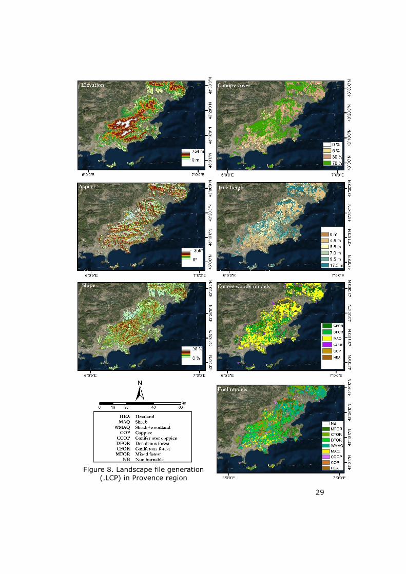
The data-set used in the study (provided by IRSTEA) contains an .LCP
file with typical topography, vegetation, and dead and living fuel
distribution along Provence’s region. A map composite (Figure 8) of
all elements are presented. All these data have been collected during
several studies from 2006 to 2012, generally from May to October
(Ganteaume et al. 2009; Curt et al. 2011; Schaffhauser et al. 2011;
Schaffhauser et al. 2012a).The last study was conducted in 2011-
2013 by the PhD student Thibaut Fréjaville although the research
remains unpublished.. It includes three topographic raster layers
together with canopy height (6 classes from 0 m up to 17.5 m),
canopy cover (4 classes ranging from 0 to 70%), custom fuel model
(9 classes including 1 non-burnable) and the coarse woody model (6
classes) data. The custom fuel model (.FMD) includes vegetation
type, fuel’s code, fuel model name, characteristic dead fuel’s load,
fuel depth, initial dead/ live fuel moisture and moisture of extinction.
Original data is derived from ca. 20-30 field surveys for each fuel
model. Because of the confidence intervals are rather slow, the
values of fuel load and fuel depth are mean values. Dead and living
fuel moisture percentages have been standardized to the fuel
moisture scenarios proposed by FARSITE.
FARSITE exports both vector files (ArcView shapefile format) and
raster (GRID ASCII format) files. Likewise explicit front-fire behaviour
computation such as rate of spread (m/min), reaction intensity
(kW/m2), fire-line intensity (kW/m), flame length (m) and heat per
area (kJ/m2) have been exported.
Chapter 3
29
Figure 8. Landscape file generation
(.LCP) in Provence region

Methodology
30
3.2.3. LPJ-GUESS-FARSITE
The following process-based meta-model sketch illustrates the
ingredients for a unique and novel approach, which should contribute
to a better understanding of the relationship between fire regimes
within the climate system and its influence on the vegetation-
dynamics (see Figure 9). Note that the fire behaviour calculated in
FARSITE impacting the vegetation in LPJ-GUESS-SPITFIRE was not
achieved in this thesis.
Figure 9. Conceptual diagram LPJ-GUESS-FARSITE

Chapter 3
31
3.3. Model’s set up
3.3.1. Assessing the variable and parameters
selection from LPJ-GUESS-SPITFIRE
As a starting point the output data selection was carried out by using
LPJ-GUESS-SPITFIRE model (Thonicke et al. 2010) in order to
evaluate how many parameters can be used as data input for the
explicit fire behaviour FARSITE model (Finney 2004). Target
parameters for the study are mostly based on the vegetation-related
modules.
Firstly, the technique was based on the analysis of input data
required by FARSITE: what data are either compulsory or optional,
metric units required, file format as well as the file extension needed
(table enclosed at Annexe 7.5). Secondly, there was an assessment
of the logic behind the model’s code for each state variable
(structures such as litter, fuel loading or canopy cover) and process
of interest (functions such as increase of biomass or fuel moisture
variations). The goal was to evaluate the adaptable variables and
parameters into FARSITE.
LPJ-GUESS framework includes different modules interrelated
representing performance of plant phenology and growth, population
dynamics, migration, soil organic matter dynamics (SOM) (Smith et
al. 2001) and fire dynamics, model developed by Thonicke et al.
(2010). Fire.cpp, growth.cpp, guess.cpp, somdynam.cpp,
vegdynam.cpp codes plus the initializer guess.ins.txt were studied to
be able to search for suitable variables, related constants and units
utilized. In order to keep the parameter selection as clear as possible,
a sub-classification by theme was carried out (table-summary
included in Annexe 7.6):
3.3.1.1. Fuel loading, SAV, Mx and fuel depth
The aboveground litter pool of each patch is divided into a number of
state variables according to tissue (leaf and wood) and PFTs. In LPJ-
GUESS-SPITFIRE, the living biomass becomes dead fuel when either
turnover or mortality transforms it into litter. Different fuel’s
diameters (based on time lag concept, point 2.3.2) are defined by
multiplying allometric relations. The product separates leaf from

Methodology
32
woody litter: fuel_1hr_total (leaves and twigs), fuel_10hr_total (small
branches), fuel_100hr_total (large branches) and fuel_1000hr_total
(boles or trunks). The application of a conversion factor from dry-
mass to carbon in the first three fuel classes resulted in dead fuel
loading (gDM C/m2). Uniquely 1hr,10hr and 100hr fuel loading are
taken into account since only they influence ROS (Rothermel 1972;
Pyne et al. 1996). Additionally, live grass fuel loading (LiveH) was
calculated in dry-mass basis (gDM/m2) taking into account the grass
phenology simulated in vegdynam.cpp. The thickest fuel class
(representing trunks and boles, fuel_1000hr_total) characterized the
live woody (LiveW) loading (gC/m2). However, due to the fact that
LPJ only burns dead fuel and ignores living non-leaf fuel, identical
values provided by IRSTEA have been used.
The Surface-to-volume (SAV) ratios are constant values (cm2/cm3)
for each fuel class. Different SAV are represented by sigma_1hr,
sigma_10hr, sigma_100hr, sigma_1000hr and sigma_grass. The fact
that SPITFIRE used fixed values for all types of fuel is cumbersome
since each custom fuel model in FARSITE requires a specific SAV ratio
for fuel 1h, LiveH, LiveW; whereas fuel 10h and fuel 100h remain
constant (reviewed in point 2.4.3). In this sense, both models fully
agree with respects to the latter assumption.
Litter flammability moisture factor (so-called litterme) is prescribed
as a constant parameter for trees, shrubs and grasses (i.e. PFT
specific). Litterme establishes the benchmark at which the fire does
not spread. The specific value of moisture of extinction (Mx) is
represented by the variable char_moistfactor. It changes over time
depending on fuel moisture and NI. FARSITE requires an explicit
moisture of extinction value for each custom fuel model.
Heat content (kJ/kg) is constant for both living and dead fuels.
Despite the fact that FARSITE requires a specific heat content value
for each custom fuel model, the variability is fairly small, therefore
LPJ has generalized it to 18000KJ/Kg. Even though fuel depth (cm) is
not explicitly computed by LPJ-GUESS-SPITFIRE, it can be easily
calculated by dividing total oven-dry fuel load (dead_fuel, gDM/m2)
by oven-dry particle density (char_dens_fuel_ave, in kg/m3).

Chapter 3
33
3.3.1.2. Fuel moisture
Fuel moisture in LPJ-GUESS-SPITFIRE is estimated based on Nesterov
Index (Lehsten et al. 2010; Thonicke et al. 2010). A litter moisture
index weighed per each dead fuel class is computed (dlm and
dlm_grass). No fuel moisture output from living wood is performed.
3.3.1.3. Stand tree parameters
Parameters related to standing trees have a direct influence over the
crown fire performance. Stand tree height can be directly interpreted
from LPJ-GUESS. It is the height from the soil to the top of the
canopy. On the other hand, crown base height did not have a straight
translation in the framework. However, its calculation simply required
a multiplication of the proportional crown’s length to the total tree
height (both measured in m). Crown bulk density (kg/m3), which
gives a volumetric measurement of the tree canopy weight, is not
explicitly calculated by LPJ. Finally, tree canopy cover (%) is defined
by foliar projective cover (fpc_tree) under full leaf cover as a fraction
of the modelled area. Grass cover is also calculated following the
same procedure.
3.3.2. Assessing initializers parameters at which LPJ-GUESS-SPITFIRE needs to be run
Since FARSITE performs explicit behaviour of fire events, it requires
the conditions before ignition. For this reason the goal is to get
outputs from LPJ as close as possible to FARSITE’s inputs dataset.
Five important parameters in LPJ's set-up needed careful
consideration: (1) temporal frame, (2) number of patches (npatch),
(3) fire return interval (fixreturnfireinterval), (4) the PFT which are
present/absent and (5) burning day (fixburnday).
3.3.2.1. Temporal frame
A model initializer document (guess_ins.txt) was set-up in such a way
that during 1000 years LPJ performed a spin-up period. In this period
of time, vegetation composition and its structure as well as soil and
litter carbon pools reached an equilibrium. An equilibrium that
included vegetation’s dynamics, the ecological succession of the PFT
and the impacts due to disturbances. The spin-up period is followed
by 30 years of the so-called historical phase. Historical data

Methodology
34
established the temporal frame in which post-analysis of LPJ outputs
have been conducted.
3.3.2.2. Number of patches
An evaluation of the required number of patches was performed in
order to get a compromise overview of between computational effort
and model stability. The more patches, the higher the amount of
replicates, the lower is the variability of the mean value. For my
work, a number of 100 patches seemed to be ideal, since the results
were stable and the time for calculation was suitable.
3.3.2.3. Fire return interval
The fire return interval parameter defines the period of time between
fire events. This parameter was included in SPITFIRE for testing
purposes. The model also allows stochastic fire occurrence
(fixrandfirereturninterval) even though this option was neglected
since there is no control over the process itself. Fire return interval
directly affects the vegetation dynamics such as succession stage,
PFT presence before/after fire as well as the performance of variables
such as living and dead fuel loading, stand height, crown base height
or canopy cover. Depending on how these parameter is set up, a
completely different vegetation composition is modelled. According to
Curt et al. (2013) the study area shows a fire return interval of 22
years for shrubs, 24 years for pine forest and 27 years for oak forest.
The areas burned from 1 up to 2 times from 1960 to 2010. This
benchmark suggested a suitable time-frame of 25 years fixed-return-
fire-interval.
3.3.2.4. PFT
LPJ-GUESS-SPITFIRE version 2008 computes 20 different PFTs. Since
the study area focusses on Mediterranean conditions, calculating all
of them would increase simulation time and storage efforts for the
results unnecessarily. Once the coordinates have been adjusted,
preliminary runs in LPJ were simulated (from 1 to 100 patches along
10, 20, 30, 40, 50 and 60 return fire intervals) in order to assess the
typical PFT environment at Provence region. None of the boreal PFT
like pLSE, BES, Bet_pub, Pic_abi or Pin_syl were present. Also
temperate types such as Bet_pen, Car_bet Pop_tree, Abi_alb and
tropical C4 grasses were disabled from the initialization's file.
Chapter 3
35
3.3.2.5. Fixburnday
For simplification purpose, 1st of August (day 213 of the year) was
selected as fixed burning day. Disregarding stochastic fire ignition
during any other time periods, the model allowed to keep more
control over the vegetation’s succession. It was also noticed from
literature that the greatest percentage of fire disturbance in Provence
occurs during the summer periods (Schaffhauser et al. 2011; Curt et
al. 2013). LPJ-GUESS-SPITFIRE burned the 100 patches selected.
3.3.3. Code’s implementation in LPJ-GUESS-
SPITFIRE
In order to perform the analysis planned, alterations on the model’s
code were indispensable. With the original structure of the model, an
evaluation in such detail as the one attempted would not be possible.
For this reason, an implementation of the code was carried out:
1. Identification of year of occurrence during the simulation run. This
could be done including the printf functionality within guess.cpp
module. It helped in the understanding of the time-frame during
modelling (Annexe 7.7, point 1).
2. Implementation of eight new variables (crown base height, fuel
depth and fuel moisture 1h, 10h, 100h, flame_length,
flame_residence and heat_per_area) which can be calculated
directly from SPITFIRE's code. The first five variables are required
as input by FARSITE. Crown base height is calculated from the
multiplication of tree height and crown length proportion. Fuel
depth derives from dead load fuel (1h+10h+100h) divided by the
fuel's density (Pyne et al. 1996). Following the same structure
used by Thonicke et al. (2010) for fuel moisture calculation
(composite estimation of moisture content for 1h, 10h, 100h
fuels), a decision of splitting up the calculation for each specific
fuel class was taken (Annexe 7.7, point 2). On the other hand, the
incorporation of these three fire behaviour new variables allowed
the comparison of outcomes between models. Both equations are
prescribed from Andrews (1986).
3. The addition of printf (“on-the-fly”) commands for each of the
target’s variables, both included in fire.cpp and growth.cpp. Printf
statements allowed variable’s identification and anomalies’ check
together with the understanding of their performance from one
year to the next (Annexe 7.7, point 3).
Methodology
36
4. After having analysed some of the output generated, it could be
observed that the spin-up time (1000y) plus historical phase
(30y) did not match with time sequence from the variable's
calculation (point 3). It was noticed that fuel-related
characteristics were calculated only if a fire event occurred. This
fact is directly related to fixfirereturninterval parameter. In order
to keep track of the overall behaviour of such variables, it was
vital to induce fire.cpp module run during non-fire years as well.
For this purpose, the loop which involved whole computation of
fire parameters and processes has been moved down in the code,
allowing fire-related calculations even if there is no fire
phenomena. The reason behind it is in the interest of keeping
daily/yearly track of dead and living fuel loading, fuel moisture,
fuel depth, moisture of extinction and tree-related characteristics
(Annexe 7.7, point 4).
5. LPJ-GUESS-SPITFIRE does calculate all variables as a whole,
summarizing all PFT per patch at the same time. To deal with the
original configuration was challenging because it did not specify
what is what or where the estimations came from. The analysis
could derive into misinterpretation from the outcomes generated.
For this reason, the variable’s selection was separated by “PFT-
specific”. This means that instead of managing average values,
each of the variables are calculated based on specific
PFTs/species. The methodology required a declaration for all
variables based on array lists with 20 spaces (20 for each possible
PFT).
In order not to interfere in the regular set-up of calculations from
LPJ-GUESS-SPITFIRE, all functions, loops and variable’s
interrelation along the code were mimicked. For instance, a dual
version from the same routine has been performed: no PFT- and
PFT-specific. Before carrying out any analysis of the results, a test
was done to see if the outputs with all PFT actually calculated the
same values as PFT specific. As a result, it was verified that dead
fuel 1h,10h, 100 h, live grass fuel loading, and fuel depth were
calculated summarizing all PFT. (See Annexe 7.14).
6. Similar to the stated in point 5, the addition of a fire behaviour
routine “PFT specific” was developed in order to assess how
individual species burn on the same patch. For instance, the
implementation allows subsequent comparison of SPITFIRE,
FARSITE and LPJ-SPITFIRE simulations per vegetation type. A
clear relationship between PFT affected by fire and its ROS, FLI,
IR, HPA and FLM associated is more enlightening than a mixture
of averaged outputs.
Chapter 3
37
7. Next step was based on automatic generation of outputs into .txt
format using fprintf functions (instead of printed “on the fly”).
This procedure allowed posterior data analysis in Excel and R.
Three different themes were developed (Annexe 7.7, point 6):
First of all the fuel-related variables in fire.cpp. Each line
contains patch ID, year, day, foliar projective cover (tree and
grass), dead fuel loading (1hr, 10hr, 100hr and 1000hr), live-
grass fuel loading, fuel depth, moisture of extinction, Nesterov
Index and fuel moisture (1hr, 10hr, 100hr and grass). Some
constraints in the output design were included, such as the
writing of only last 30 years (historical phase) as well as only
the day before, during and day after fire event.
Secondly, the fire behaviour variables, also taken from fire.cpp
module. For instance propagating flux, reaction intensity,
influence of wind speed, fuel bulk density, packing ratio, heat
of pre-ignition, forward and backward ROS, fire duration,
forward and backward distance, number of fire, fire danger
index, Byram’s fire-line intensity, area, flame length and heat
per area were exported.
Finally, since the information regarding standing tree cannot
be calculated on individual basis from the fire.cpp module, a
third implementation regarding tree allometry within
growth.cpp module was included. Subsequently, yearly
records from number of patches, individual height, crown
length proportion, leaf, sapwood and heart mass plus DBH
were performed.
The cited outputs were created both for PFT non-specific/specific. Unit
conversion was indispensable for almost all variables in both codes
since FARSITE utilises different units of measurement to those from
SPITFIRE. The unit transformations were applied only within the
fprintf function instead of inside each routine.
3.3.4. Code’s modification in LPJ-GUESS-
SPITFIRE.
A detailed analysis over the fire.cpp code has revealed differences in
heat of pre-ignition and packing ratio formulas with regards to the
presentation of the model in Thonicke et al. (2010). At least two
discrepancies with reference to the parameterization proposed by
Rothermel (1972) and revised in Albini (1976a) have been detected
(Annexe 7.8, point 1). Changes in heat of pre-ignition (Q_ig) together
with beta-optimum (beta_opt) parameterization were introduced

Methodology
38
following Pyne et al. (1996). Reformulation of fire spread equation in
Metric Units was prescribed by Wilson (1980). These two parameters
have a direct effect over ROS and IR. ROS at the same time
influences the so called Bryan's fire-line intensity (FLI) and therefore
FML as well. It was hypothesized a decrease in ROS’s simulations.
Q_ig is dividing ROS, hence an increment in Q_ig will lead to
decrease in ROS, thus decrease in FML and FLI as well.
On the other hand, the formula of the area calculated in fire.cpp
showed discrepancies between pixel degree size introduced and the
area calculation found. At least one order of magnitude seemed to be
overestimated (Annexe 7.8, point 2). In theory 1º grid cell along the
Equator, where the latitude is 0, should perform an area of 1 e10 km2.
But 1.23 e9 km2 was calculated instead. The cited pixel degree
parameter expects an area of approximately 4 km2 (this value should
be reduced due to the latitude by Earth deformation). However,
preliminary calculations of 35.98 km2 were obtained instead. This
area is key variable for the simulation of burning emission.
3.3.5. Assessing parameters at which FARSITE
needs to be run
The dataset from Provence provided by IRSTEA has many different
vegetation and fuel types. Therefore a very specific target area of
study was selected as ignition point. The goal was to mimic the
conditions estimated by LPJ-GUESS as much as possible. Mainly
shrublands (Quer_coc) and grasslands (C3_grass) as well as lower
amount of forest (Quer_Ile, Quer_pub, Quer_pub and Fag_syl) have
been simulated in LPJ-GUESS over Provence. For this reason the
target area in FARSITE was only based primarily on MAQ together
with WMAQ and DFOR fuel models. Fire under COP and CCOP
presence have been neglected since man-made management
activities can induce to bias.
Since one of the aims is to achieve meaningful and realistic
comparison between model’s calculations, the conditions in both
programs should be as simple and similar as possible. Since LPJ-
GUESS-SPITFIRE does not take into account topography, elevation,
slope and aspect in its estimations, FARSITE’s data set has been
transformed to a completely flat surface. For this purpose, the
landscape calculator tool included in FARSITE v4.1 was utilized.
Chapter 3
39
3.3.5.1. Set parameters
The grid cell resolution was based on 100m (1 cell=0.1 km2). Time
step computed fire behaviour performance each 30 minutes. The
perimeter resolution was set to 60 m and the distance resolution to
30 m. FARSITE’s technical reference from User guide always
recommends values lower than grid cell resolution. Fire barriers such
roads or rivers were not taken into account. Nevertheless, the data-
set already neglected land uses such as build-up areas and water
bodies. The simulation was set only to one day of duration on 1st of
August, mimicking LPJ-GUESS-SPITFIRE set up.
The ignition point was set into MAQ fuel model. The coordinates
assigned to the raster cell were 2º33’ longitude- 45º89’ latitude
(Projected Coordinate System: NTF Lambert II étendu; Projection:
Lambert Conformal Conic). Crown fire computation was enable
following Finney, 1998 method instead of Scott and Reinhardt (2001)
method.
3.3.5.2. Input data
For the comparison LPJ-GUESS-SPITFIRE vs FARSITE, the Landscape
(LCP) file generation comprised:
Fuel: (21) HEA, (32) MAQ, (33) WMAQ, (24) COP, (26) CCOP,
(37) DFOR, (38) CFOR, (39) MFOR and (99) Non burnable.
Coarse woody: (21) HEA, (32) MAQ, (24) COP, (26) CCOP, (37)
DFOR and (38) CFOR.
Canopy cover: 0, 5, 30 and 70 %. Stand height: 0, 4.5, 5.5, 7.0,
9.5 and 17.5 m. Crown base height: 1.5 m (constant). Further
descriptions in (Curt et al. 2011; Schaffhauser et al. 2011)
Elevation, slope and aspect set to zero. Similarly occurs with
crown bulk density and duff loading.
FARSITE project file have included:
Landscape file (LCP).
Fuel adjustments set to 1 (i.e. no change over regular fuel
models).
Fuel moistures 1h, 10 h, 100h, LH and LW. These are the
standardized fuel moisture scenarios proposed by FARSITE in
summer since almost all fires in Provence are in summer (Curt,
T., personal communication, 2014). The values are consistent in

Methodology
40
comparison with field measurements calculated by Curt et al.
(2011) and also with fuel moisture models described in Salis
(2007).
Custom fuel model 21, 32, 33, 24, 26, 37, 38, 39 and 99 (Code,
fuel loading, SAV, fuel depth, Mx and heat content. Data collected
from different field campaigns, further description (Ganteaume et
al. 2009; Curt et al. 2011; Curt et al. 2013)
Coarse woody model 21, 32, 24, 26, 37 and 38 (Diameter, fuel
loading, heat content, sapwood and heartwood density and
moisture). The coarse woody debris were measured in the field
between spring and summer of 2012 and 2013 (PhD student
Thibaut Fréjaville, remains unpublished).
Adaptation of SQL weather and wind data. Instead of using only
data provided by weather stations close to the study area, a
combination of SQL global data (utilized by LPJ) and Hyeres’
weather station has been carried out. The reason behind it, is to
use as close weather and wind data as LPJ. Hence temperature,
precipitations and wind speed are exactly the same. However,
some assumptions were mandatory, since FARSITE needs higher
detailed weather data in comparison to LPJ-GUESS-SPITFITE.
Therefore minimum temperature and maximum temperature were
assumed to be 0600 hr and 1500 hr respectively, maximum and
minimum humidity were “standardized” from relative humidity.
Elevation was set to 85 m above the sea level. Wind direction
135º and cloud cover 0 %.
3.4. Introducing LPJ-GUESS outputs as inputs in FARSITE: LPJ-GUESS-FARSITE’s germ
LPJ-GUESS-FARSITE implies the embedment of vegetation related
outcomes from LPJ-GUESS within FARSITE fire behaviour model. In
order to assess the performance of LPJ-GUESS-FARSITE, the next
logical step was to compare the outcomes in fire behaviour from the
three models: LPJ-GUESS-SPITFIRE, FARSITE and LPJ-GUESS-
FARSITE. The comparison lies within all vegetation types (i.e. non
PFT-specific) computed in LPJ-framework. Since there is not a direct
connexion between all LPJ-GUESS outputs and FARSITE inputs,
several assumptions have been taken into account.
The selection of 100 patches/replicates simulated in LPJ under the
effect of 25 years fire return interval was utilized for the design of a
synthetic landscape in Provence region. Synthetic landscape refers to
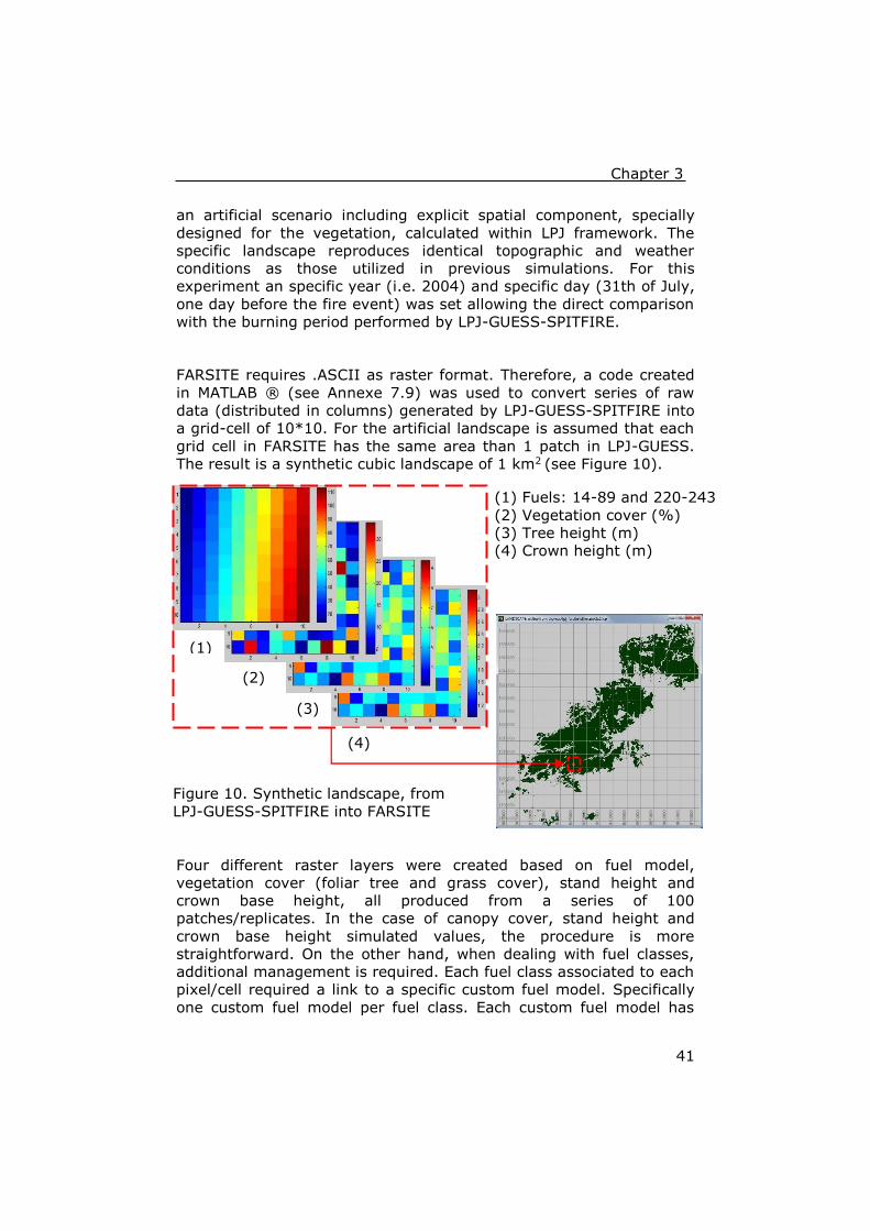
Chapter 3
41
an artificial scenario including explicit spatial component, specially
designed for the vegetation, calculated within LPJ framework. The
specific landscape reproduces identical topographic and weather
conditions as those utilized in previous simulations. For this
experiment an specific year (i.e. 2004) and specific day (31th of July,
one day before the fire event) was set allowing the direct comparison
with the burning period performed by LPJ-GUESS-SPITFIRE.
FARSITE requires .ASCII as raster format. Therefore, a code created
in MATLAB ® (see Annexe 7.9) was used to convert series of raw
data (distributed in columns) generated by LPJ-GUESS-SPITFIRE into
a grid-cell of 10*10. For the artificial landscape is assumed that each
grid cell in FARSITE has the same area than 1 patch in LPJ-GUESS.
The result is a synthetic cubic landscape of 1 km2 (see Figure 10).
Four different raster layers were created based on fuel model,
vegetation cover (foliar tree and grass cover), stand height and
crown base height, all produced from a series of 100
patches/replicates. In the case of canopy cover, stand height and
crown base height simulated values, the procedure is more
straightforward. On the other hand, when dealing with fuel classes,
additional management is required. Each fuel class associated to each
pixel/cell required a link to a specific custom fuel model. Specifically
one custom fuel model per fuel class. Each custom fuel model has
Figure 10. Synthetic landscape, from
LPJ-GUESS-SPITFIRE into FARSITE
(1) Fuels: 14-89 and 220-243
(2) Vegetation cover (%)
(3) Tree height (m)
(4) Crown height (m)
(4)
(3)
(2)
(1)

Methodology
42
different fuel loading, fuel depth, Mx and fuel moisture. According to
Scott and Burgan (2005), the user is allowed to use any number
between 1-256. The latter means that the model allow up to 256
different combinations of typical fuel related variables. However,
there is the exception of those already committed to the original
Anderson’s fuel models; numbers 1-13 (Anderson 1982), and those
identified with the Scott and Burgan new fuel models. For example,
91-93, and 98-99 are identified as non-burnable. Therefore, all in all,
the approach followed included fuels from fuel model 14 to 89 and
from 220 to 243. The cited four raster layers (10*10) are
subsequently inserted in FARSITE model (see Figure 10).
The Landscape (LCP) file generation comprised:
Fuel: 100 fuel models representing each patch/replicate.
Canopy cover, stand height and crown base height were
introduced in each raster cell. In this experiment, mean values
were not taken into account.
Elevation, slope and aspect set to zero. A similar situation occurs
with crown bulk density and duff loading.
FARSITE project (FPJ) included:
Landscape file (LCP) created above.
Fuel adjustments set to 1 (i.e. no change over regular fuel
models).
Fuel moistures for each patch (1h, 10 h, 100h, LH and LW) taken
from each patch. LPJ-GUESS-SPITFIRE does not calculate LW,
hence the same value from IRSTEA dataset was kept. On the
other hand, all fuel moisture lower than 2% had to be
standardized to 2% since this is the minimum value accepted by
FARSITE.
Custom fuel model for each patch (Code, fuel loading, SAV, fuel
depth, Mx and heat content). SAV 10-h and 100-h, similarly to
LW, were also preserved from fuel models provided by IRSTEA.
Coarse woody model were disregarded. Due to the species’
mixture in each patch, to specify a particular coarse woody model
for each patch was not possible.
Adaptation of SQL weather and wind data, followed the same
procedure as explained in 3.3.5.
For this simulation, set parameters such as grid cell resolution,
simulation duration as well as ignition point preserved the
experimental design presented in point 3.3.5.1.
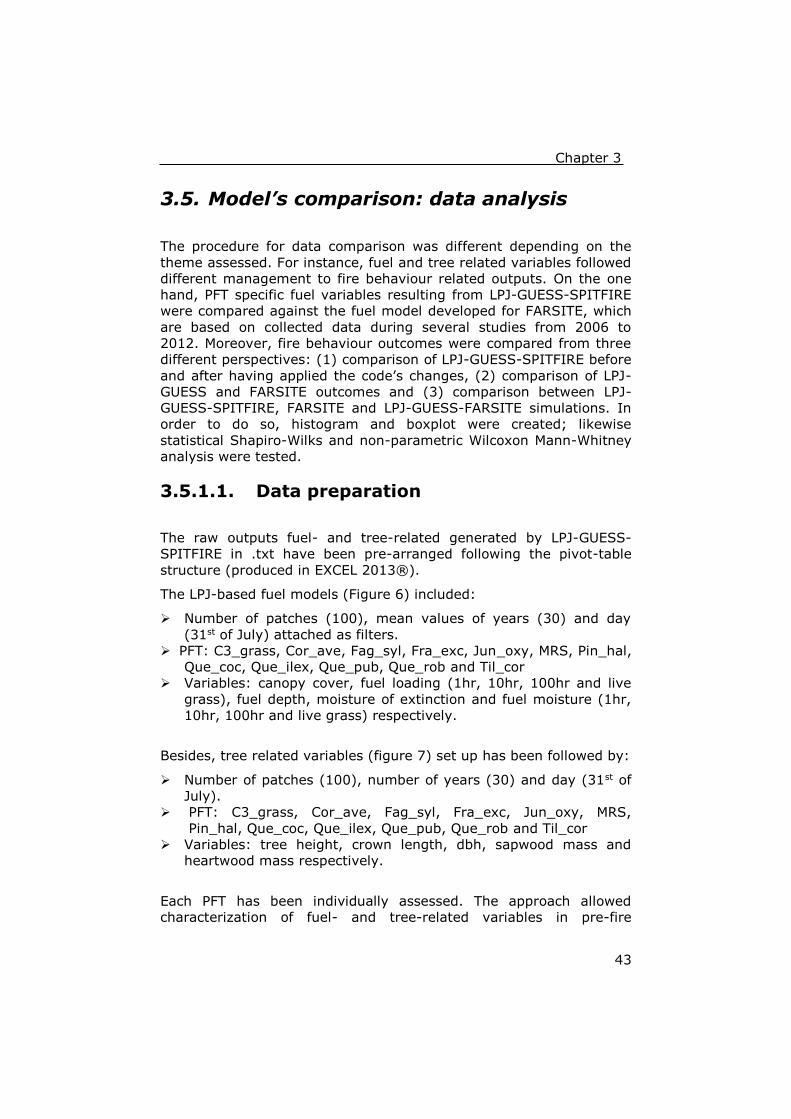
Chapter 3
43
3.5. Model’s comparison: data analysis
The procedure for data comparison was different depending on the
theme assessed. For instance, fuel and tree related variables followed
different management to fire behaviour related outputs. On the one
hand, PFT specific fuel variables resulting from LPJ-GUESS-SPITFIRE
were compared against the fuel model developed for FARSITE, which
are based on collected data during several studies from 2006 to
2012. Moreover, fire behaviour outcomes were compared from three
different perspectives: (1) comparison of LPJ-GUESS-SPITFIRE before
and after having applied the code’s changes, (2) comparison of LPJ-
GUESS and FARSITE outcomes and (3) comparison between LPJ-
GUESS-SPITFIRE, FARSITE and LPJ-GUESS-FARSITE simulations. In
order to do so, histogram and boxplot were created; likewise
statistical Shapiro-Wilks and non-parametric Wilcoxon Mann-Whitney
analysis were tested.
3.5.1.1. Data preparation
The raw outputs fuel- and tree-related generated by LPJ-GUESS-
SPITFIRE in .txt have been pre-arranged following the pivot-table
structure (produced in EXCEL 2013®).
The LPJ-based fuel models (Figure 6) included:
Number of patches (100), mean values of years (30) and day
(31st of July) attached as filters.
PFT: C3_grass, Cor_ave, Fag_syl, Fra_exc, Jun_oxy, MRS, Pin_hal,
Que_coc, Que_ilex, Que_pub, Que_rob and Til_cor
Variables: canopy cover, fuel loading (1hr, 10hr, 100hr and live
grass), fuel depth, moisture of extinction and fuel moisture (1hr,
10hr, 100hr and live grass) respectively.
Besides, tree related variables (figure 7) set up has been followed by:
Number of patches (100), number of years (30) and day (31st of
July).
PFT: C3_grass, Cor_ave, Fag_syl, Fra_exc, Jun_oxy, MRS,
Pin_hal, Que_coc, Que_ilex, Que_pub, Que_rob and Til_cor
Variables: tree height, crown length, dbh, sapwood mass and
heartwood mass respectively.
Each PFT has been individually assessed. The approach allowed
characterization of fuel- and tree-related variables in pre-fire

Methodology
44
conditions along 30 years’ time-series. Mean values and standard
deviation were calculated from all the patches. The presentation of
the data follows the same structure as custom fuel model provided by
IRSTEA (Table 5). The current format guarantees a direct and
interchangeable way of connecting fuel outputs (LPJ-framework) to
fuel models (FARSITE). This comparison demanded mean values,
even though the current set up allows one fuel model per PFT per day
of the year over 30 years’ time.
3.5.1.2. Statistical analysis
A statistical analysis was carried out using R software package (R
Development Core Team, 2005). All data was separated into
independent datasets derived from LP-GUESS-SPITFIRE, FARSITE and
LPJ-GUESS-FARSITE models respectively. ROS, IR, FLI, FML and HPA
were tested. A normality analysis was performed following Shapiro-
Wilks Test. Due to the related samples ranked (i.e. ordinal data that
can be put in order) and the fact that the sample distribution does
not follow a normal distribution, a non-parametric Wilcoxon Mann-
Whitney Test was utilized (Quinn and Keough 2002). Pair-related
thematic variables from both models were analysed consecutively.
The null hypothesis stated that both populations have identical
distribution functions and mean, and it is ultimately identified by the
U-test significance.
3.5.1.3. Histogram and boxplot comparison
The data pre-processed obtained from LPJ-GUESS-SPITFIRE and
FARSITE has been plotted using R software (R Development Core
Team, 2005) together with ggplot2 package. Regarding the script
code written in R (Annexe 7.14), data could be entered, plotted and
statistically tested afterwards. ROS, IR, FLI, FML and HPA simulated
from both models have been assessed. The First experiment
compared the performance of LPJ-GUESS-SPITFIRE before and after
the code’s change. For the second experiment, FARSITE and LPJ-
GUESS-SPITFIRE were compared. Finally, a third set of comparisons
analysed all three models against each other.
In order to do so, a set of five histograms per experiment together
with comparative boxplots (including Min, 1st Quartile, Media, Mean,
3rd Quartile, Max and outliers) was created. Analysing the
appearance of each data-set allowed the analysis of the shape,
variability and centre of the data. Outcomes from FARSITE, LPJ-

Chapter 3
45
GUESS-SPITFIRE and LPJ-GUESS-FARSITE were combined in the
same data-frame even though the sample size was different in each
case.

46

47
4. Results
The results derived from the assessment presented in the
methodology section are disclosed in the following unit. Results are
structured in two different themes. The first theme deals with the
model’s set up, exemplifying the impact of fire return interval over
the composition of the vegetation. The influence over the LPJ-GUESS-
SPITFIRE code’s modification is also presented. The second theme
shows, in first place, the comparison of fuel- and tree- related
variables calculated from LPJ-framework against the field data
provided by IRSTEA; secondly, the fire behaviour results obtained
both from FARSITE vs LPJ-GUESS-SPITFIRE and FARSITE vs LPJ-
GUESS-SPITFIRE vs LPJ-GUESS-FARSITE.
4.1. Models’ set up
4.1.1. Assessing initial parameters at which LPJ
needs to be run
The estimations from LPJ-GUESS show a strong (cause-effect)
dependence between PFT presence and the fix fire return interval, i.e.
fire regime. A comparative Leaf Index Area (LAI= leaf area / ground
area, m2 / m2), Biomass (CMASS, kgC/m2) and Net Primary
Production (NPP, kgC/m2 year) are shown per fix fire return interval
in Figure 11 and 12. The stacked-area-plots show the vegetation
dynamics whilst there is an increase of 10 years interval between fire
recurrences, ranging from 10 up to 60 years return interval. The
simulations displayed are based on 100 patches/replicates along 30
years of historical data. Spin up time was neglected. Furthermore
Carbon Fluxes emitted by fires (CFLUX, g emission / kg biomass
burned) are enclosed as a supplement, linking up fire occurrence and
PFT fluctuations.
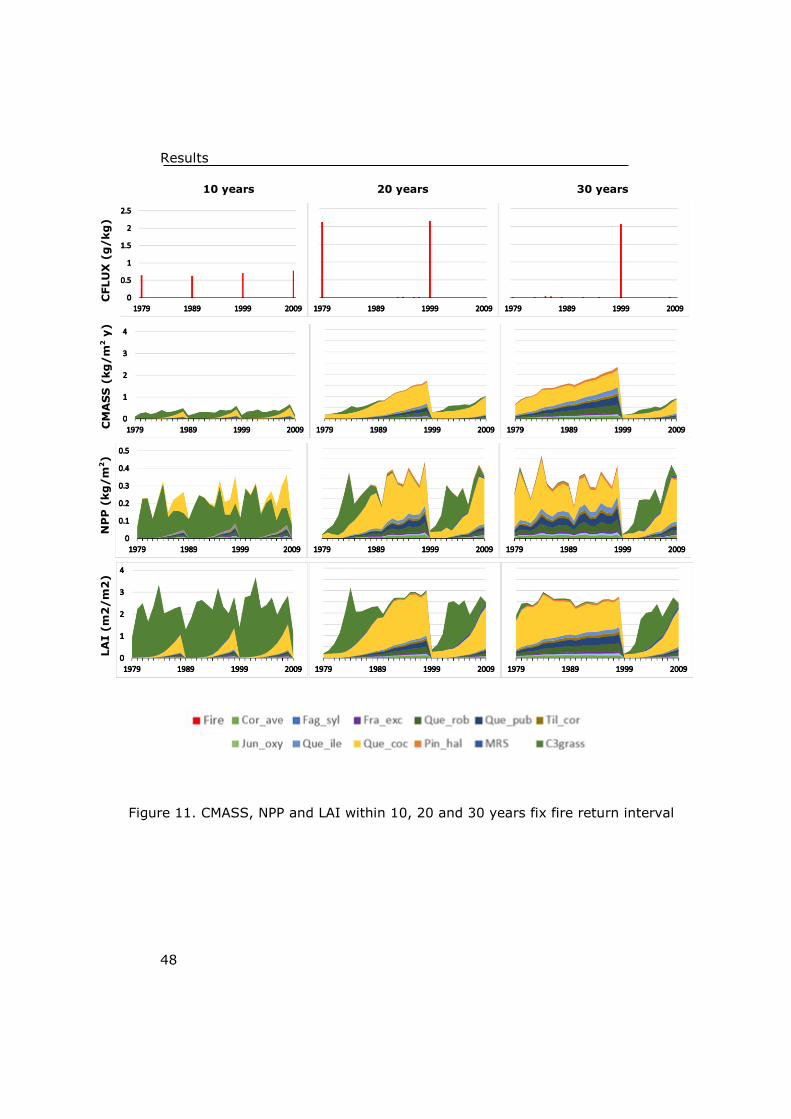
Results
48
NP
P (
kg
/m
2)
LA
I (
m2
/m
2)
Figure 11. CMASS, NPP and LAI within 10, 20 and 30 years fix fire return interval
CM
AS
S (
kg
/m
2 y
)
10 years 30 years
CFLU
X (
g/kg
)
()
20 years
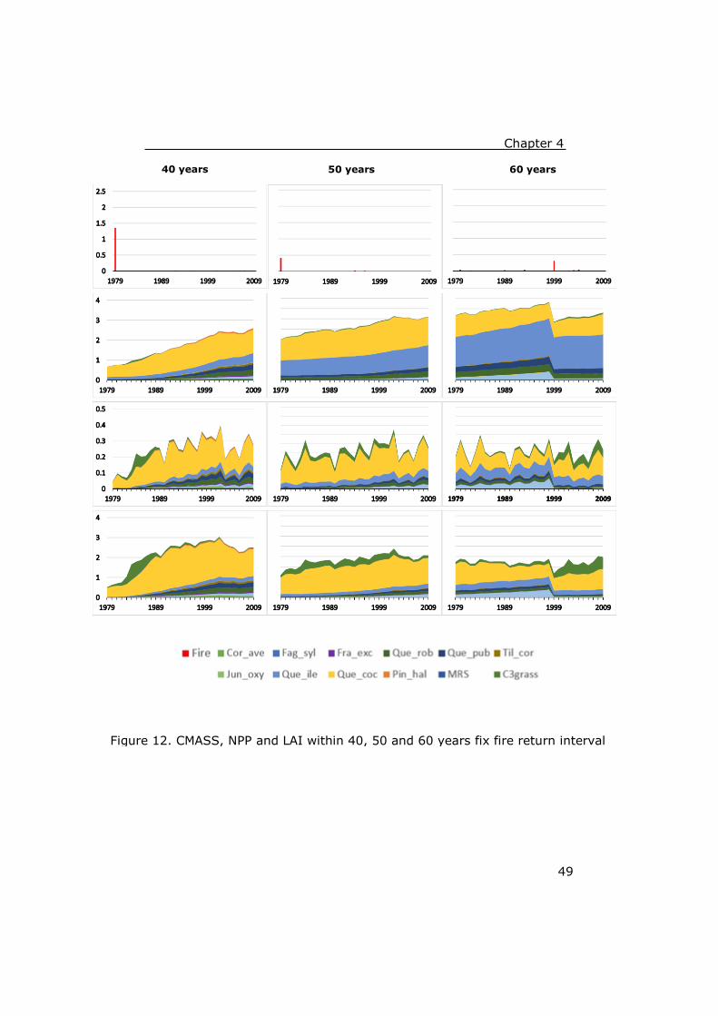
Chapter 4
49
Figure 12. CMASS, NPP and LAI within 40, 50 and 60 years fix fire return interval
50 years 60 years 40 years
Results
50
The results suggest great facility of establishment for non-woody
species within short fix fire return intervals. Grasses C3 at first and
Quercus coccifera subsequently, appear predominantly under such
kind of successional stages. On the contrary, woody species like
Quercus Ilex barely appear in these conditions. It would seem that
under such higher recurrence fire interval, they need more time to
settle. An increase of 30 years fix fire return interval brings a new
successional scenario. Although Quercus coccifera is still
predominant, Quercus Ilex, Quercus pubescens or Quercus robur
begin a partial colonization of the patches. The PFT show high
resilience/sensitivity to fire events since LAI, CMASS and NPP
decrease abruptly after disturbance. Moreover, an immediate
increase in grasses and Quercus coccifera is estimated after fire
occurrence.
However, woody species show a much higher tendency to establish
within 40 fix fire return intervals. Fagus sylvatica, Tilia cordata and
Pinus halepensis behave as the previous mentioned species. The
weight of these PFT in the ecosystem increases at the same time as
the fire regime experiences higher gaps between fix fire return
intervals. 50 and 60 years simulations shown how woody species are
highly more prominent than shrublands or grasslands. Fagus
sylvatica, Quercus Ilex, Quercus pubescens, Quecus robur together
with Quercus coccifera in a lower extent, are predominant.
Additionally, individual remarks to each thematic outputs are
presented. CMASS seems to follow an homogenous increase in
comparison with the oscillating behaviour previously shown by NPP
along the time. An example of the first is the smooth and fluent
increase of biomass from 30-40-50 to 60 years of fix fire return
interval’s series. On the other hand, NPP fluctuates relatively often
and such behaviour could be caused by the seasonal and inter-annual
weather’s variability experienced by the vegetation. Unexpected
results were simulated regarding the fires within 40-50-60 years fix
return interval. The intensity of the fires seems to decrease with
respect to the increased fire recurrence. Only one big fire has
occurred along 40 years’ case. The following two (50 and 60 years
fire recurrence) show a significant decrease of the emissions.
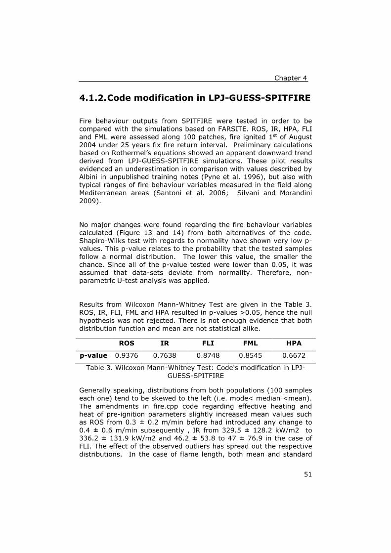
Chapter 4
51
4.1.2. Code modification in LPJ-GUESS-SPITFIRE
Fire behaviour outputs from SPITFIRE were tested in order to be
compared with the simulations based on FARSITE. ROS, IR, HPA, FLI
and FML were assessed along 100 patches, fire ignited 1st of August
2004 under 25 years fix fire return interval. Preliminary calculations
based on Rothermel’s equations showed an apparent downward trend
derived from LPJ-GUESS-SPITFIRE simulations. These pilot results
evidenced an underestimation in comparison with values described by
Albini in unpublished training notes (Pyne et al. 1996), but also with
typical ranges of fire behaviour variables measured in the field along
Mediterranean areas (Santoni et al. 2006; Silvani and Morandini
2009).
No major changes were found regarding the fire behaviour variables
calculated (Figure 13 and 14) from both alternatives of the code.
Shapiro-Wilks test with regards to normality have shown very low p-
values. This p-value relates to the probability that the tested samples
follow a normal distribution. The lower this value, the smaller the
chance. Since all of the p-value tested were lower than 0.05, it was
assumed that data-sets deviate from normality. Therefore, non-
parametric U-test analysis was applied.
Results from Wilcoxon Mann-Whitney Test are given in the Table 3.
ROS, IR, FLI, FML and HPA resulted in p-values >0.05, hence the null
hypothesis was not rejected. There is not enough evidence that both
distribution function and mean are not statistical alike.
Table 3. Wilcoxon Mann-Whitney Test: Code's modification in LPJ-
GUESS-SPITFIRE
Generally speaking, distributions from both populations (100 samples
each one) tend to be skewed to the left (i.e. mode< median <mean).
The amendments in fire.cpp code regarding effective heating and
heat of pre-ignition parameters slightly increased mean values such
as ROS from 0.3 ± 0.2 m/min before had introduced any change to
0.4 ± 0.6 m/min subsequently , IR from 329.5 ± 128.2 kW/m2 to
336.2 ± 131.9 kW/m2 and 46.2 ± 53.8 to 47 ± 76.9 in the case of
FLI. The effect of the observed outliers has spread out the respective
distributions. In the case of flame length, both mean and standard
ROS IR FLI FML HPA
p-value 0.9376 0.7638 0.8748 0.8545 0.6672

Results
52
deviation remain identical, i.e. 0.4 ± 0.2 m. In contrast, the HPA
mean value decreased from 2607.5 ± 1837.1 to 2413.9 ± 1247.5
kJ/m2. The variable tends to be less spread distributed compared
with ROS, FLI or IR. This is also translated into lower estimated
maximum values.
The initial assumption hypothesized a decrease of FLI and FML in case
the ROS could decay. In fact such variation did not take place.
Similarly befalls with HPA, dependent on IR.
Figure 13. Boxplots:
Code's modification in
LPJ-GUESS-SPITFIRE

Chapter 4
53
Fig
ure
14.
Perf
orm
ance d
iffe
rences f
or
RO
S,
FLI,
FM
L,
IR a
nd H
PA r
epre
sente
d a
s c
hanges in h
isto
gra
ms d
ue t
o c
ode's
modific
ation in L
PJ-
GU
ESS-S
PIT
FIR
E
F
i
g
u
r
e
6
.
P
e
r
f
o
r
m
a
n
c
e
d
i
f
f
e
r
e
n
c
e
s
f
o
r
R
O
S
,
F
L
I
,
F
M
L
,
I
R
a
n
d
H
P
A
r
e
p
r
e
s
Figure 5. Performance differences for ROS, FLI, FML, IR and HPA represented
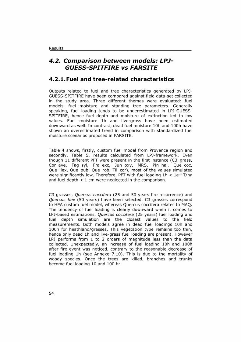
Results
54
4.2. Comparison between models: LPJ-GUESS-SPITFIRE vs FARSITE
4.2.1. Fuel and tree-related characteristics
Outputs related to fuel and tree characteristics generated by LPJ-
GUESS-SPITFIRE have been compared against field data-set collected
in the study area. Three different themes were evaluated: fuel
models, fuel moisture and standing tree parameters. Generally
speaking, fuel loading tends to be underestimated in LPJ-GUESS-
SPITFIRE, hence fuel depth and moisture of extinction led to low
values. Fuel moisture 1h and live-grass have been estimated
downward as well. In contrast, dead fuel moisture 10h and 100h have
shown an overestimated trend in comparison with standardized fuel
moisture scenarios proposed in FARSITE.
Table 4 shows, firstly, custom fuel model from Provence region and
secondly, Table 5, results calculated from LPJ-framework. Even
though 11 different PFT were present in the first instance (C3_grass,
Cor_ave, Fag_syl, Fra_exc, Jun_oxy, MRS, Pin_hal, Que_coc,
Que_ilex, Que_pub, Que_rob, Til_cor), most of the values simulated
were significantly low. Therefore, PFT with fuel loading 1h < 1e-3 T/ha
and fuel depth < 1 cm were neglected in the comparison.
C3 grasses, Quercus coccifera (25 and 50 years fire recurrence) and
Quercus Ilex (50 years) have been selected. C3 grasses correspond
to HEA custom fuel model, whereas Quercus coccifera relates to MAQ.
The tendency of fuel loading is clearly downward when it comes to
LPJ-based estimations. Quercus coccifera (25 years) fuel loading and
fuel depth simulation are the closest values to the field
measurements. Both models agree in dead fuel loadings 10h and
100h for heathland/grasses. This vegetation type remains too thin,
hence only dead 1h and live-grass fuel loading are present. However
LPJ performs from 1 to 2 orders of magnitude less than the data
collected. Unexpectedly, an increase of fuel loading 10h and 100h
after fire event was noticed, contrary to the reasonable decrease of
fuel loading 1h (see Annexe 7.10). This is due to the mortality of
woody species. Once the trees are killed, branches and trunks
become fuel loading 10 and 100 hr.

Chapter 4
55
Low values of fuel loading lead to underestimation of fuel depth and
Mx since both are fuel loading-dependents. Fuel depth records do not
follow the same homogeneity as fuel loading along the time. There
are years with either very low or directly no-fuel depth at all
(probably due to the impact of fire events). Moisture of extinction
estimations, on the other hand, seem unrealistic because a litter
flammability moisture factor of 20% was assigned to grasses and a
30% to shrubs and forest. The results only indicate reasonable
ranges of performance (i.e. 20-30% Mx) if there is enough fuel
loading, otherwise it leads to unviable values.
Fuel moisture shows a different behaviour compared to preceding
variables. LPJ-GUESS-SPITFIRE tends to overestimate fuel moisture
10h and 100h compared to FARSITE fuel models. Nonetheless, fuel
moisture 1h and live grass have shown very low moisture instead,
almost null. Although zero is an overstatement, it seems reasonable
due to high dryness performed by the model in summer periods.
Tree related parameters take into account vegetation cover, i.e. foliar
projective coverage for grasses and trees, together with tree height
and crown height. An overview between models is presented in Table
6. MAQ and Que_coc show a notable agreement regarding the
associated tree variables. Meanwhile HEA and C3_grasses count null
tree and crown height as expected (life form grass is different than
life form tree or shrub). However, canopy cover differs. LPJ-GUESS-
SPITFIRE provides the equivalent of canopy cover for grasses.
FARSITE does not take it into account, and for this reason it remains
as zero. DFOR and Que_ile displayed the highest disagreement. A
canopy cover of 70% introduced by FARSITE data-set opposed the
scarce 5% calculated by LPJ. Even though the calculations of fix fire
return interval are set to 50years, the underestimation seems
obvious. Tree and crown height estimated in LPJ are also higher than
in observations. Nonetheless, the results are not clear if the
vegetation type is miscellaneous/mixed.
Results
56 Table
4.
Custo
m f
uel m
odel colle
cte
d f
rom
Pro
vence r
egio
n
Ve
ge
tati
on
Ty
pe
So
ilF
ue
l
Mo
de
l
De
pth
(cm
)M
x (
%)
1h
10
h1
00
hliv
e1
h1
0h
10
0h
HW
He
atl
an
d21
Ca/S
iH
EA
0.4
50
02.5
827.0
030.0
09.0
010.0
011.0
080.0
090
Scru
b32
Si
MA
Q3
0.8
0.1
3.2
80.0
020.0
09.0
010.0
011.0
080.0
090
Scru
b w
oo
dla
nd
33
Si
WM
AQ
3.8
0.9
0.2
3.2
220.0
020.0
09.0
010.0
011.0
080.0
090
Co
pp
ice
24
Ca/S
iC
OP
61.5
0.3
3.5
753.0
028.0
09.0
010.0
011.0
0100.0
0120
Co
nif
er
ov
er
co
pp
ice
26
Ca/S
iC
CO
P8.4
1.0
50.3
91.6
933.0
025.0
09.0
010.0
011.0
0100.0
0110
De
cid
eo
us f
ore
st
37
Si
DF
OR
71.8
0.3
310.0
025.0
09.0
010.0
011.0
0100.0
0120
Co
nif
ero
us f
ore
st
38
Si
CF
OR
6.7
51.1
30.2
72.6
10.0
023.0
09.0
010.0
011.0
0100.0
0120
Mix
ed
fo
rest
39
Si
MF
OR
7.6
51.1
30.2
73.4
710.0
025.0
09.0
010.0
011.0
0100.0
0120
No
n b
urn
ab
le99
* H
eat
conte
nt=
18000 k
J/Kg f
or
all
fuel m
odels
co
de
_F
MF
ue
l lo
ad
(t.
ha
-1)
Init
ial D
FM
C (
%)
LF
MC
(%
)
Table
5.
Custo
m f
uel m
odel genera
ted b
y L
PJ-
GUESS-SPIT
FIR
E
Ve
ge
tati
on
Ty
pe
So
il
Fu
el
Mo
de
l
(P
FT)
De
pth
(cm
)M
x (
%)
1h
10
h1
00
hliv
e1
h1
0h
10
0h
HW
Te
mp
era
te g
rasse
s1
-C
3_
gra
ss
0.4
30.0
00.0
00.0
039
4.3
02.6
021.4
5100.0
0100.0
07.1
7-
Te
mp
era
te s
hru
bla
nd
2-
Qu
e_
co
c1.8
40.2
20.7
80.0
000
28.3
124.5
70.0
043.1
030.7
7-
-
Te
mp
era
te g
rasse
s1
-C
3_
gra
ss
0.4
90.0
00.0
00.0
040
4.9
42.5
422.8
5100.0
0100.0
06.7
6-
Te
mp
era
te s
hru
bla
nd
2-
Qu
e_
co
c1.5
70.1
40.5
20.0
000
22.3
617.8
30.0
050.3
137.3
2-
-
Te
mp
era
te fo
rest
3-
Qu
e_
ile
x0.1
80.0
50.1
70.0
000
4.0
83.6
11.8
272.8
761.3
3-
-
* H
eat
conte
nt=
18000 k
J/Kg f
or
all
fuel m
odels
25y
50y
co
de
_F
MF
ue
l lo
ad
(t.
ha
-1)
Init
ial D
FM
C (
%)
LF
MC
(%
)
Table
6.
Tre
e-re
lated v
ariable
s c
om
parison
FA
RS
PIT
FA
RS
PIT
FA
RS
PIT
HEA
C3_gra
s
sM
AQ
Que_coc
DFO
RQ
ue_ilex
Ca
no
py
co
ve
r (
%)
010.4
85
6.6
470
5
Tre
e h
eig
ht (
m)
00
4.5
2.1
29.5
11.2
4
Cro
wn
he
igh
t (
m)
00
1.5
0.7
11.5
3.7
4
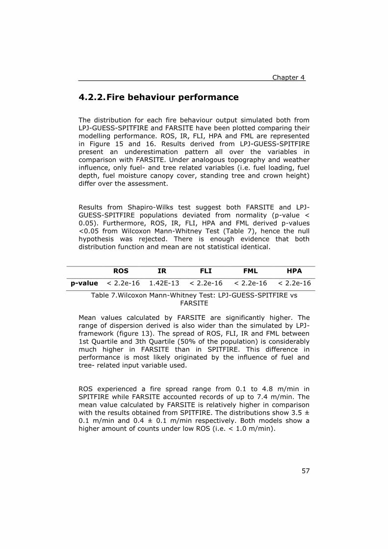
Chapter 4
57
4.2.2. Fire behaviour performance
The distribution for each fire behaviour output simulated both from
LPJ-GUESS-SPITFIRE and FARSITE have been plotted comparing their
modelling performance. ROS, IR, FLI, HPA and FML are represented
in Figure 15 and 16. Results derived from LPJ-GUESS-SPITFIRE
present an underestimation pattern all over the variables in
comparison with FARSITE. Under analogous topography and weather
influence, only fuel- and tree related variables (i.e. fuel loading, fuel
depth, fuel moisture canopy cover, standing tree and crown height)
differ over the assessment.
Results from Shapiro-Wilks test suggest both FARSITE and LPJ-
GUESS-SPITFIRE populations deviated from normality (p-value <
0.05). Furthermore, ROS, IR, FLI, HPA and FML derived p-values
<0.05 from Wilcoxon Mann-Whitney Test (Table 7), hence the null
hypothesis was rejected. There is enough evidence that both
distribution function and mean are not statistical identical.
ROS IR FLI FML HPA
p-value < 2.2e-16 1.42E-13 < 2.2e-16 < 2.2e-16 < 2.2e-16
Table 7.Wilcoxon Mann-Whitney Test: LPJ-GUESS-SPITFIRE vs
FARSITE
Mean values calculated by FARSITE are significantly higher. The
range of dispersion derived is also wider than the simulated by LPJ-
framework (figure 13). The spread of ROS, FLI, IR and FML between
1st Quartile and 3th Quartile (50% of the population) is considerably
much higher in FARSITE than in SPITFIRE. This difference in
performance is most likely originated by the influence of fuel and
tree- related input variable used.
ROS experienced a fire spread range from 0.1 to 4.8 m/min in
SPITFIRE while FARSITE accounted records of up to 7.4 m/min. The
mean value calculated by FARSITE is relatively higher in comparison
with the results obtained from SPITFIRE. The distributions show 3.5 ±
0.1 m/min and 0.4 ± 0.1 m/min respectively. Both models show a
higher amount of counts under low ROS (i.e. < 1.0 m/min).

Results
58
In the case of IR, the histogram plotting FARSITE calculations shows
a core with many of the pixel counts presenting high intensities. As a
result, FARSITE’s mean and standard deviation values (780.2 ±
451.2 kW/m2) overestimate substantially the ones from LPJ-
framework (336.2 ± 131.9 kW/m2). However, IR shares more
common counts from both models than any other fire behaviour
variable assessed (especially within the range 100-400 kW/m2).
SPITFIRE simulates FLI with values ranging from 6 to 674.3 kW/m. In
contrast, FARSITE’s results have fluctuated from 4.9 to 773.9kW/m.
Similarly to ROS, the spreading of the distribution remains dispersed
in comparison with SPITFIRE. FLI simulated in SPITFIRE reached a
mean intensity of 47 ±76.9 kW/m against the 357.1± 231.3 kW/m
calculated in FARSITE.
FML fluctuated from 0.2 to 1.6 m based on SPITFIRE simulations
against the 0.2 to 2.25 meters predicted by FARSITE. In terms of
distribution’s variation, FARSITE resulted in a 1.3 ± 0.6 m in
comparison with only 0.4 ± 0.2m in SPITFIRE. Both models show
Figure 15. Boxplots:
LPJ-GUESS-SPITFIRE vs FARSITE
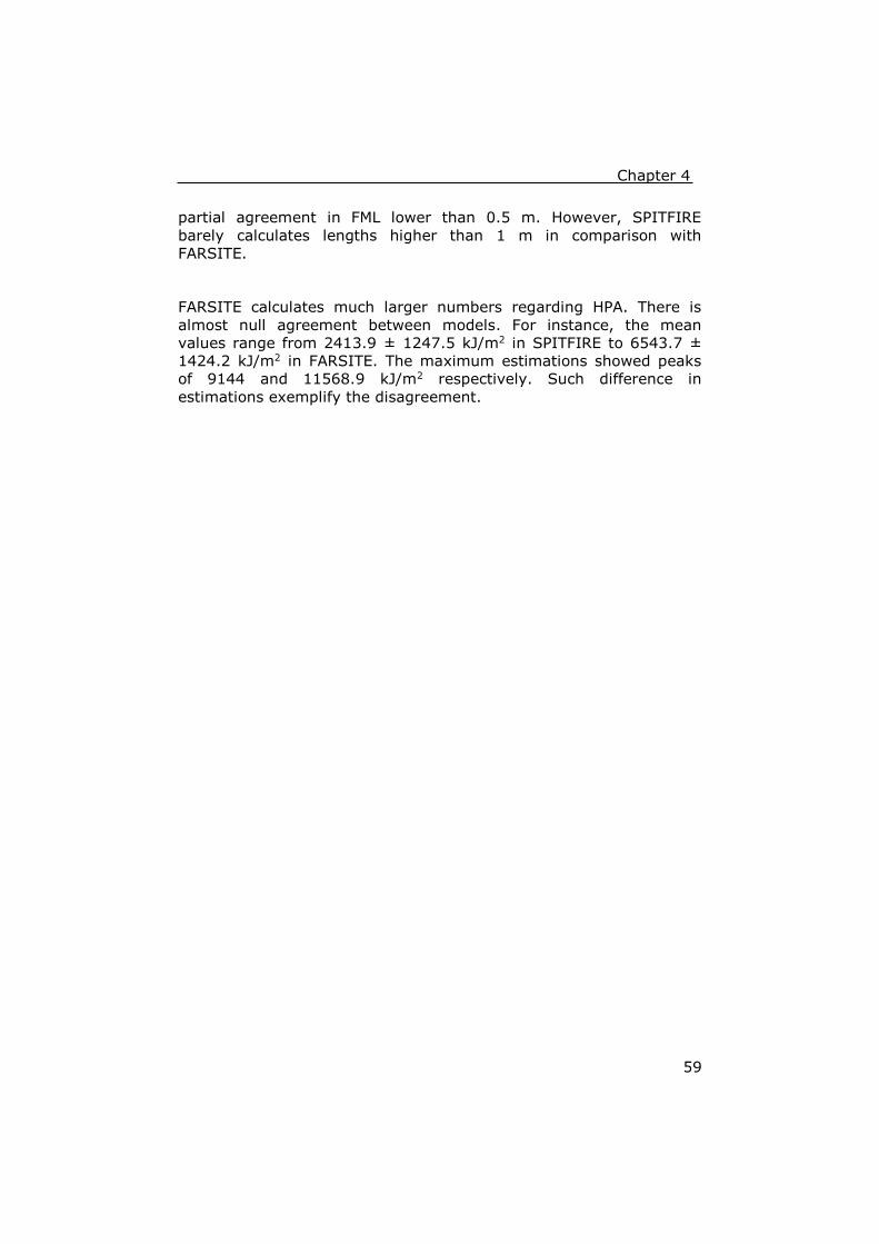
Chapter 4
59
partial agreement in FML lower than 0.5 m. However, SPITFIRE
barely calculates lengths higher than 1 m in comparison with
FARSITE.
FARSITE calculates much larger numbers regarding HPA. There is
almost null agreement between models. For instance, the mean
values range from 2413.9 ± 1247.5 kJ/m2 in SPITFIRE to 6543.7 ±
1424.2 kJ/m2 in FARSITE. The maximum estimations showed peaks
of 9144 and 11568.9 kJ/m2 respectively. Such difference in
estimations exemplify the disagreement.
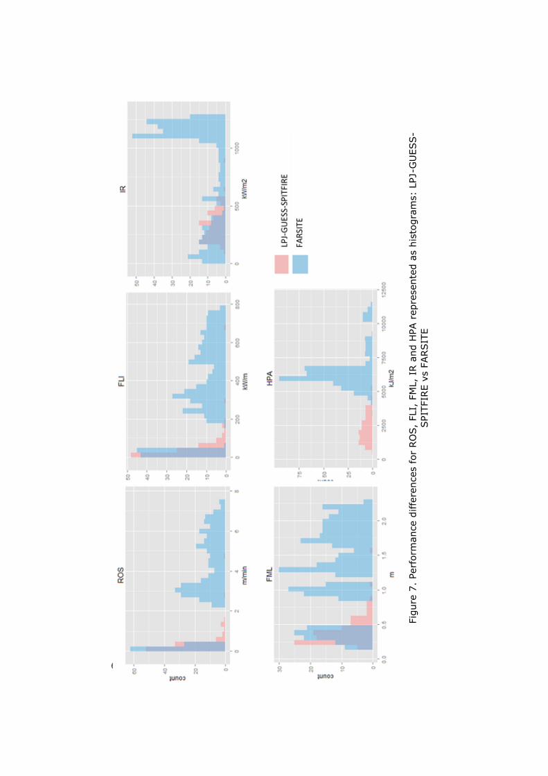
Results
60
Fig
ure
7.
Perf
orm
ance d
iffe
rences f
or
RO
S,
FLI,
FM
L,
IR a
nd H
PA r
epre
sente
d a
s h
isto
gra
ms:
LPJ-G
UESS-
SPIT
FIR
E v
s F
ARSIT
E

Chapter 4
61
4.3. Introducing LPJ-GUESS outputs as inputs in FARSITE: LPJ-GUESS-FARSITE’s germ
The vegetation resulted from 100 patches simulated in LPJ-GUESS-
SPITFIRE were incorporated as input data in FARSITE. This approach
aimed at evaluating the model’s performance under identical fuel-
and tree-input conditions. The distribution for each output-variable
simulated from SPITFIRE, FARSITE and LPJ-FARSITE was plotted in
order to compare each individual performance. ROS, IR, FLI, HPA and
FML are represented in figure 17 and 18. Generally speaking, the
results derived from the embedded LPJ-GUESS-FARSITE presented a
wider range of fire behaviour estimations all over the variables
compared to LPJ-GUESS-SPITFIRE.
Results from Shapiro-Wilks test suggested both populations’ model
deviated from normality (p-value < 0.05). According to Wilcoxon
Mann-Whitney Test, none of the variables evaluated resulted in p-
values >0.05, hence the null hypothesis was rejected. There is
enough evidence to state that both distribution function and means
are not statistical identical.
The main distinctive trait observed is the slight increase of ROS,
moderate growth of IR, FLI and FML together with an atypical very
high range of HPA in comparison with LPJ-GUESS-SPITFIRE (results
represented in figure 15 and 16). It is interesting to see how both
models performed differently under the same set of input data, i.e.
climate, topography and vegetation.
Fire spread presented a mean value of 0.7 ± 0.3 m/min. In no case
ROS exceeds 2 m/min. The range of values are similar to LPJ-GUESS-
SPITFIRE, although slightly higher. It is also evident the narrowed
dispersion shape of the distribution.
LPJ-GUESS-FARSITE has moderately increased the range of mean
estimation of IR, FLI and FML to 698.3 ± 223.2 kW/m2, 150.7 ±67.7
kW/m and 0.8 ± 0.2 m respectively. The cited distributions have
shown a slightly higher spread due to the appearance of outliers,
which led to maximum records of 1547.2 kW/m2, 442.87 kW/m and
1.55 m length.

Results
62
Figure 17. Boxplots: LPJ-
GUESS-SPITFIRE vs
FARSITE vs LPJ-GUESS-
FARSITE
HPA is the variable with highest degree of change from model to
model. Since the increment of IR was not that large, such range of
values were unexpected, simulating even higher intensities than
FARSITE’s calculations. A mean value 11986.6 ±1289.4 kJ/m2
contrasted with the only 2413.9 ± 1247.5 kJ/m2 simulated by LPJ-
GUESS-SPITFIRE.
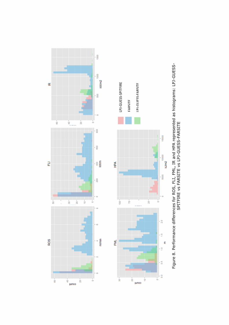
Chapter 4
63
Fig
ure
8.
Perf
orm
ance d
iffe
rences f
or
RO
S,
FLI,
FM
L,
IR a
nd H
PA r
epre
sente
d a
s h
isto
gra
ms:
LPJ-G
UESS-
SPIT
FIR
E v
s F
ARSIT
E v
s L
PJ-
GU
ESS-F
ARSIT
E
LPJ-GUESS-SPITFIRE
FARSITE
LPJ-GUESS-FARSITE

Results
64

65
5. Discussion
In this section the results are discussed. The overall aim for this
thesis was to assess a potential embedment of vegetation dynamics
(LPJ-GUESS) into an explicit fire behaviour model (FARSITE). In order
to do so, the main questions were focused on the possibility of LPJ-
GUESS to simulate characteristic vegetation from Provence (France);
how realistically both LPJ-GUESS-SPITFIRE and LPJ-GUESS-FARSITE
performed fire spread as well as fire intensity-related estimations;
and if any improvement could be made.
The following sections will go into further detail of (1) how initializers
parameters have affected the presence/absence of the different PTFs;
(2) how much fuel- and tree-related variables agree compared to
field measurements; (3) how code's refinements have affected fire
behaviour results; (4) how much agreement actually model
comparison has shown, but also with field observations and finally,
(5) some recommendations about how the models could be further
developed.
5.1. Model’s set up
5.1.1. Assessing initializers parameters at which LPJ needs to be run
Fire is a key disturbance factor in Mediterranean areas. Wildfire
impacts and shapes the structure, composition and dynamics of the
ecosystems (Pausas 1999). The existence of different fire return
intervals (i.e. fire regimes or fire recurrence) led to different
vegetation types in Mediterranean areas (Curt et al. 2011;
Ganteaume et al. 2011; Schaffhauser et al. 2011; Schaffhauser et
al. 2012a; Curt et al. 2013).

Discussion
66
5.1.1.1. Fire return interval and succession
stage
Generally speaking, fire affects directly the successional status of the
ecosystem. More precisely, the cited change over the ecosystem is
called secondary succession since the plants colonize an existing
substrate after most or all biomass has been destroyed by a fire
disturbance. Fire clears the patches (in LPJ-GUESS-SPITFIRE) or
extensive areas (in real life) and resets succession locally.
Furthermore it establishes new frames of competence between
species. The strategies followed by rural species (R) (in frequently-
disturbed environments) allow a more rapid adaptation to the
ecosystem after disturbance than that of their competitors (C). An
example is fire-prone areas, i.e. within fix fire return intervals lower
than 20 years. It obstructs plant’s survival due to insufficient time to
recruit from seeds (Pausas 1999; Curt et al. 2009). Therefore,
resprouting species such as Quercus coccifera, Quercus Ilex or
Quercus suber is likely to see benefits under such conditions
(Schaffhauser et al. 2011). In order to survive, plants need to adapt
to the environment which surrounds them through the development
of a specific strategy.
An expected (natural) sequence represents the replacement of R-type
species (for example C3_grass) by C-type species at the same time
that light, water and nutrient availability at soil surface declines. For
instance, shade-intolerant pioneer trees (species like Cor_ave,
Jun_oxy and MRS) can be initially established, followed by shade-
tolerant trees afterwards (Car_bet, Fag_syl, Fra_exc, Que_rob,
Que_pub, Til_cor, Que_ile, Que_coc and Pin_hal). According to
Gordon (2008); Lehsten (2013); Schlesinger and Bernhardt (2013)
changes in vegetation’s structure and its stage within the succession
directly affect functions such as NPP, LAI and CMASS. On the one
hand CMASS tends to increase over time after the fire event,
accumulating the biomass as sapwood and heartwood mass in tree
stems/trunks. On the other, LAI and NPP tend to increase for the first
few years but quickly saturate. The decrease in NPP is likely driven by
the increased maintenance costs of old trees and (sometimes)
reduced soil nutrient status. In fact, these different patterns fully
agree with the results obtained (4.1.1). Short fire regimes lead to low
CMASS together with high NPP and LAI. The tendency changes at the
same time that fix fire return interval increases.

Chapter 5
67
Figure 9. Succession stage dependent of fire recurrence
(Schaffhauser et al. 2011)
Schaffhauser et al. (2011) have assessed how the
abundance/quantity and dimensions of trees and shrubs vary
inversely to increasing fire return interval owing to selective mortality
of trees. If fire recurrence increases, a reduction of the plant’s
vertical profile (i.e. tree height) together with canopy cover, stand
basal area and litter depth can be observed. A complementary
diagram supporting these relations is shown in Figure 19. Ganteaume
et al. (2009) also suggested a significant reduction of canopy cover
due to an increase of fire occurrences (i.e. decrease of fire return
interval).
Indeed, such behaviour can be elucidated from results simulated by
LPJ-GUESS in comparison to figure 19. Within short fire regimes at
early stages of succession only grassland (C3 grasses) and shrubland
(Quercus coccifera) showed up. Estimations from the model
suggested rather low woody biomass in overall terms together with
high LAI and NPP from Quercus coccifera and C3 grasses under 10
and 20 years fix fire return intervals. Ganteaume et al. (2009)
discusses the possibility of insufficient time from seed-producers
species to restock seed bank. For instance, it could promote
resprouting species such as Quercus coccifera, Quercus Ilex or
Quercus suber (Pausas 1997; Delitti et al. 2005). Quercus coccifera
has been described as a very fire-resilient plant specie, mostly due to

Discussion
68
its spread root system (Canellas and Miguel 1998). In Figure 19, cited
resprouting species are represented by Cistus (medium maquis),
Erica or Arbutus spp (both high maquis), homologue to Quercus
coccifera in LPJ-GUESS. Opposed to these scenarios, 30, 40, 50 and
60 years show an increased weight of the woody species such as
Quercus Ilex, Quercus robur, Quercus pubescens, Pinus halepensis,
Fagus sylvatica and Fraxinus excelsior. The role of these PFT grows as
return fire interval increases. Quercus coccifera and C3 grasses are
still present but in much lower proportions.
5.1.1.2. Presence of PFTs
C3 grasses, Quercus coccifera and Quercus Ilex are three PFT
representative of three different sequences of post-fire succession in
Provence. The fact that C3 grasses and Quercus coccifera
predominate at low fire intervals is consistent with observations on
field. The optimum fire interval for these species has been found
within 10-30 years from field studies. Woody types such as Quercus
Ilex predominate at fire intervals > 30-50 years, so the results match
field measurements (Schaffhauser et al. 2011; Schaffhauser et al.
2012b, a). Actually, in the eastern part of Provence, under similar
conditions, Quercus suber grows instead of Quercus Ilex, and
Erica/Cistus spp instead of Quercus coccifera. Curt et al. (2013) have
summarized the main characteristic vegetation types with dominant
species in the study area. Two different classifications exist
depending on soil composition. However, LPJ-GUESS does not
differentiate between either siliceous/acidic and limestone substrates.
For instance, LPJ-GUESS seems to oversimplify vegetation types as
well as it tends to model PFT as if the study area was in limestone-
derived soils instead of over siliceous strata. One example, maquis
vegetation type represented by Erica arborea and Cistus spp (what in
theory belongs to MRS in LPJ) does not appear at all in the
simulations. Instead, Quercus coccifera, typical example of garrigue
vegetation type is widespread. Two possible explanations given to
these facts could be: (1) Quercus coccifera is more competitive than
MRS in conditions of water shortage and infertile soils and/or (2) the
concept of PFT is too fuzzy for the level of detail required, i.e. a scale
issue. Due to the mode of computation of LPJ-GUESS, the model does
not differentiate between substrates at local scales. LPJ-GUESS is not
suited for such detailed vegetation analyses since it is a global model.
In case a complete substratum is not implemented, it could be
considered that Quercus coccifera garrigue predominates everywhere
(knowing that this will be in reality only on limestone), while the
equivalent (Erica/Cistus spp) will be on acidic soils.
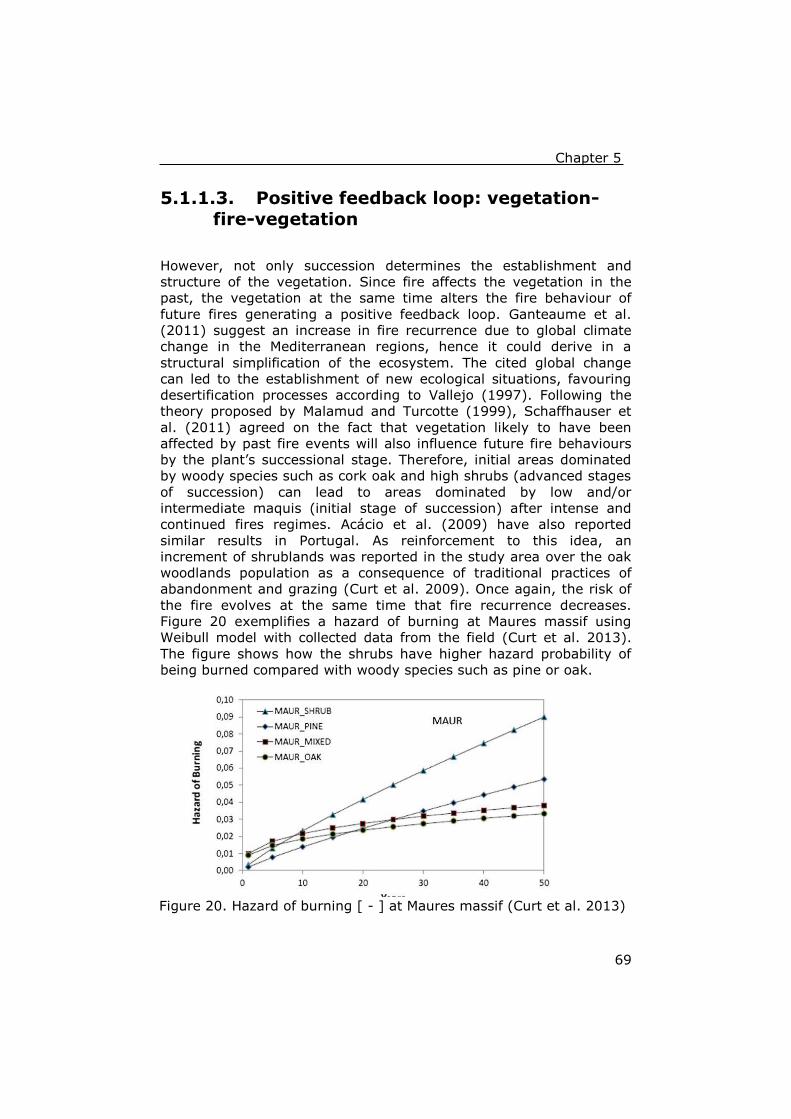
Chapter 5
69
Figure 20. Hazard of burning [ - ] at Maures massif (Curt et al. 2013)
5.1.1.3. Positive feedback loop: vegetation-
fire-vegetation
However, not only succession determines the establishment and
structure of the vegetation. Since fire affects the vegetation in the
past, the vegetation at the same time alters the fire behaviour of
future fires generating a positive feedback loop. Ganteaume et al.
(2011) suggest an increase in fire recurrence due to global climate
change in the Mediterranean regions, hence it could derive in a
structural simplification of the ecosystem. The cited global change
can led to the establishment of new ecological situations, favouring
desertification processes according to Vallejo (1997). Following the
theory proposed by Malamud and Turcotte (1999), Schaffhauser et
al. (2011) agreed on the fact that vegetation likely to have been
affected by past fire events will also influence future fire behaviours
by the plant’s successional stage. Therefore, initial areas dominated
by woody species such as cork oak and high shrubs (advanced stages
of succession) can lead to areas dominated by low and/or
intermediate maquis (initial stage of succession) after intense and
continued fires regimes. Acácio et al. (2009) have also reported
similar results in Portugal. As reinforcement to this idea, an
increment of shrublands was reported in the study area over the oak
woodlands population as a consequence of traditional practices of
abandonment and grazing (Curt et al. 2009). Once again, the risk of
the fire evolves at the same time that fire recurrence decreases.
Figure 20 exemplifies a hazard of burning at Maures massif using
Weibull model with collected data from the field (Curt et al. 2013).
The figure shows how the shrubs have higher hazard probability of
being burned compared with woody species such as pine or oak.
Discussion
70
5.1.2. Code’s modification in LPJ-GUESS-
SPITFIRE: the before and the after
According to the fire behaviour parameterization prescribed by
Rothermel (1972), subsequently revised in Albini (1976a), converted
from English into SI units (Wilson 1980) and finally re-examined by
Wilson Jr. (1982), part of the regular parameterization within fire
module (fire.cpp) has not been properly formulated. On the one
hand, Heat of pre-ignition’s (Q_ig) equation clearly mismatches the
equation shown in Thonicke et al. (2010). Although optimum packing
ratio (beta_opt) uses the same parameterization in both code and
journal article, the citations from the authors pointed out Wilson Jr.
(1982) as parameterization’s source in the other hand. Hence the
evidence suggests a more than likely new typing error in the source
code.
The modification of the code aimed at the improvement of LPJ-
GUESS-SPITFIRE fire behaviour performance. However, the results
did not suggest significant changes between ROS, IR, FLI, FML and
HPA simulations, before and after the amendment.
Beta optimum is a parameter dependent on optimum reaction
velocity which, at the same time, is a multiplier in the IR calculation.
Therefore, beta optimum also influences ROS, FLI, FML and HPA
estimations. On the other hand, the heat of pre ignition’s parameter
directly relates to ROS equation. Rate of spread is the key element in
the calculation of Byram’s Fire-line intensity, hence the flame length
is, by extension, as well. However, the expected decrease in FLI, FML
(caused by ROS,) and increase in HPA (forced by IR increment) did
not occurred.
A possible explanation of such a slight difference in the results could
be the minor weight of these two parameters in the overall
performance of the fire behaviour parameterization. For instance, an
upwards change driven by fuel loading or fuel moisture has readily
shown apparent increased results (an example of fuel moisture
influence is given in Annexe 7.11). Indeed, modifications in optimum
packing ratio do not compute large differences since the modification
falls into the order of thousandths. Nevertheless, an increment of two
orders of magnitude within the heat of pre-ignition equation ought to
derive into no trivial changes in ROS results, hence not affecting FLI
Chapter 5
71
and FML neither. The results do not shows such a difference. Perhaps
the changes only motivated the appearance of spread peaks higher
than 1m/min, increasing the variability of the simulations. The
regular set-up of SPITFIRE has shown low and homogeneously
distributed values of ROS below 0.5 m/min. Such low values are
characteristic from areas without wind and slope influence (Pyne et
al. 1996). Provence is characteristic for great influence of winds
during the summer though (Curt et al. 2013).
FARSITE estimations were used as a benchmark in order to define
what a reasonable output should look like. In addition Pyne et al.
(1996), following Albini F.A unpublished training notes, also showed
typical examples of ROS, HPA, FML and FLI under different conditions
(Annexe 7.13). Both were used for preliminary comparison of the
LPJ-GUESS-SPITFIRE’s fire behaviour results. Already this first
evaluation has shown certain signs of evident fire behaviour
underestimation’s tendency.
5.2. Comparison between models
5.2.1. Fuel and tree-related characteristics
The characterization of litter, and consequently fuel loading, as well
as fuel depth and fuel moisture is essential for a fire behaviour
assessment together with its effects (Pyne et al. 1996; Curt et al.
2011). The implementation of LPJ-GUESS-SPITFIRE’s code allowed
simulation of fuel related variables at the specific level of detail
required to compare it with field measurements. Moreover, the
development of such configuration also permitted a subsequent
connexion to FARSITE as input data. In general terms, estimations
have shown low fuel loading (Table 5), thus thin fuel depth. The
simulations of fuel moisture show very low 1h and live grass moisture
together with high 10h and100h fuel moisture (Table 5).
Nonetheless, with a suitable calibration of LPJ-GUESS-SPITFIRE, the
model would allow the development of custom fuel model following a
multi-temporal perspective. In particular, the current set up permits
one fuel model per PFT per day of the year over 30 years’ time
sequence. Normally these fuel models are set for a specific time in
specific circumstances. LPJ-GUESS-SPITFIRE offers an attractive
dynamic sense into fire behaviour modelling.
Discussion
72
5.2.1.1. Litter/fuel loading
A complementary comparison of custom fuel model CM28 developed
by Salis (2007) from data set in North of Sardinia (Italy) has revealed
a tendency to agree with respect to the fuel model developed in
IRSTEA. Similar to Provence, Sardinia’s typical vegetation is mostly
based on Mediterranean shrub as well. Salis carried out field
measurements in order to develop the custom fuel model; likewise,
researchers in IRSTEA have developed the dataset used for this
thesis. The performance of the cited fuel model against prescribed
shrubland models from the US (Anderson 1982; Scott and Burgan
2005) was assessed. The best results were obtained with regards to
the custom-homemade fuel model compared to the prescribed from
US. The fuel loading and depth fuel from CM28 is in agreement with
MAQ and WMAQ. Fuel loading 10h and 100h tend to be overestimated
in CM28 though.
When comparing the mean values of LPJ-GUESS-SPITFIRE, the 1h
and 10h fuel loads seem very low for Quer_ile (temperate forest) and
Quer_coc (shrubland), and almost null for live fuel load whereas
IRSTEA had measured values of ca. 3 T/ha. Likewise, a fuel depth of
only 2.4 cm in forest seems very low (probably this is only litter)
whereas researches carried out by IRSTEA generally have evolved in
high fuel depth in the Mediterranean. The latter is mainly because
many fuels are in understory (Ganteaume et al. 2009; Curt et al.
2011).
Litter derived from leaf and wood regarding Quercus coccifera
annually simulated by LPJ-GUESS are extensively underestimated in
comparison with observation from fieldwork carried out in Spain
regarding the same specie (Canellas and Miguel 1998). Different litter
fall rates were measured in 70, 40 and 10 years’ fire recurrence
dependent. Summing up leaf and wood litter, the study respectively
obtained 381.2, 348.5 and 257.7 kg/ha year. LPJ-framework only
simulated 173.61 kg/ha year for Quercus coccifera. This value also
underestimates results obtained in France (Rapp and Lossaint 1981).
On the other hand, typical litter fall rates in Mediterranean areas
show 250-300g/m2 for Quercus suber, 250-700g/m2 for in Quercus
Ilex whereas it is 400-500 for Pinus halapensis and 500-600 for
Mediterranean decideous oaks. (Quézel and Médail 2003; Curt et al.
2011). For the given fire recurrence (25 years), LPJ-GUESS has
estimated litter fall derived from woody species of < 1g/m2 in the

Chapter 5
73
same area. Therefore the downward tendency in simulating fuel
loading and fuel depth evidence flaws in soil organic matter and
vegetation dynamic modules instead of within the fire module. Litter
inputs, generated in growth.cpp and introduced in fire module, are
already low themselves.
The litter/fuel load of a specific area should not only directly relate to
the vegetation established. The location can also vary the production-
decomposition of combustible fuel (Olson 1963). According to Quézel
and Médail (2003), litter biomass and fuel bulk density are the result
from litter fall and its subsequent decomposition rate. Litter biomass,
and for instance fuel load degradation, depends on the level of
dryness, leaching, microbiological activity and/or fauna activity
(Olson 1963; Wright 1997; Incerti et al. 2011).
Wright (1997) even has established a cause-effect relation between
acidic/siliceous soils (i.e. low pH such as in Maures massif’s area) and
lower decomposition/mineralization rates. This kind of soils has a
characteristic small level of productivity and therefore a limited
exchange of nutrients. In Provence acidic soils are more favourable to
forest than limestone because they are a slight more fertile and have
a bit higher water capacity and less stoniness (T. Curt, personal
communication, 2014). This particular process was also noticed by
Caritat et al. (2006) regarding low fuel loadings of Quercus suber
over fertile soils.
In Wright (1997), dryness was also pointed out as an alternative
disturbance’s source influencing production of litter/fuel. It was
described how in Mediterranean areas, under water shortage/stress
conditions, woody plants tend to present high concentrations of
structural compounds (i.e. higher molecular weight particles) and low
N content. This fact potentially could slow down decomposing rates
(Castells et al. 2004; Incerti et al. 2011). More specifically, Wright
(1997) associated high concentration of tannins in species to those
better adapted to drought periods. Specifically, this was reported in
sclerophyll plants such as Quercus coccifera and Quercus Ilex. As an
example, Quercus coccifera presents a variable range of tannins,
from 123 to 312 g/kg depending on the physiological scale.
Incerti et al. (2011) have related the overestimation of litter loss rate
obtained in their simulations (i.e. underestimation of remaining leaf

Discussion
74
litter in the standing tree) with the abundance in inhibitory-structural
compounds belonging to Mediterranean species. Therefore, higher
molecular weight compounds such as tannins are most likely to lower
organic matter decomposition and mineralization rates by forming
organic matter-based complexes (Hättenschwiler and Vitousek 2000;
Castells et al. 2004).
LPJ-GUESS takes into account carbon balance in the same way as
biochemical cycle takes into account the litter decomposition
processes. However due to the coarse scale, the models do not
represent specific local conditions such as the Mediterranean region.
Persson (2013) concluded that turnover times in LPJ-GUESS-
SPITFIRE are not very representative for leaves and wood under
specific local conditions. The current study has reproduced the same
limitations.
For instance, if the cited decomposition rate of solid organic matter is
set excessively fast (i.e. time of decomposition short), the fuel
loading would lead to an unavoidable underestimation. In order to
increase the fuel loading estimations, two different approaches could
be applied:
1. A manual set up of the initialized file with one, and only one PFT
per simulation, inducing the establishment of monoculture
scenarios. Higher fuel loadings (up to 5 T/ha) and fuel depth are
reached. Nonetheless, due to competition, species and functional
types often have a more limited distribution than expected, based
on their physiological limitations. For this reason the cited
approach is rather unrealistic and its use in this thesis was
ignored.
2. based on the causal relationship between the climatic/edaphologic
conditions, and litter and soil organic matter decomposition
(Incerti et al. 2011), LPJ-GUESS allows parameter tuning
regarding turnover litter rates for leafs and wood.
Simultaneously, regarding the use of PFT-specific routine
(introduced in 3.3.3), the model performed higher fuel loading
and fuel depth simulations. In LPJ-GUESS the relation of tau
turnover times (years) for litter and soil organic matter at 10ºC
are based on Foley (1995). The original values for tau litter leaf,
root and wood (somdynamic.cpp) are all 2.85 for all PFT all over
the world. The regular set up is rather simple and not
representative of the reality. In case of an increment of
tau_litter_leaf * 5 is applied, the results obtained reflect an

Chapter 5
75
increase from 1.84 to 5.28 T/ha (fuel loading) and from 28.31 to
63.11 cm (fuel depth) regarding Quercus coccifera within 25 years
fire recurrence.
5.2.1.2. Fuel moisture
Moisture models presented by IRSTEA remain in similar ranges with
Salis (2007), agreeing in both low fuel moisture 1 h, 10 h and 100 h.
The ranges stand for 10% 11% 12% and 8% 9% 10% respectively,
i.e. vegetation is driven by water shortage conditions along the
summer. Fuel moisture estimations are probably one of the weakest
points of LPJ-GUESS-SPITFIRE. According to the results, obtained 1h-
DFMC for temperate shrubland is very low (that mean complete
desiccation), while 10h-DFMC of 43 to 100 among the fuel types
indicates that they are rather fresh, which is never the case in
Provence in summer. For instance, fuel moisture disagree
considerably with the moisture estimated in Provence and reviewed
by Salis in Sardinia. Indeed fuel moisture could be a key factor
behind such low fire behaviour performance.
An interactive peer-review of LPJ-DGVM-SPITFIRE previous to its
publication (Thonicke et al. 2010) exposed several discrepancies
regarding fuel moisture performance. For instance, Venevski (2010)
suggested flaws in simulation of fuel moisture. The author was also
involved in the development of Reg-FIRM (Venevsky et al. 2002), a
process based model which SPITFITE structure is mainly based on
(i.e. similar approach and formulations such as Nesterov Index,
Rothermel fire spread or natural/human ignition sources).
Venevski fully disagrees with the fuel moisture calculation, mostly
regarding in two aspects:
1. The nature of the equation requires a drying rate (inverse
proportions of three fuel classes’ SAV) in the order of 0.001 to
0.0001 to provide daily moisture higher than 50%. Venevski
argued that, in terms of volume, the latter assumption represents
a cubic fuel particle with SAV equal 1000 to 10000 respectively.
Hence the fuel size would have either 0.006 to 0.00006 m
(6/SAV). This theoretical framework leads to fuel particle too
small. Even for a hypothetical higher fuel moisture, the particles
sizes would be even smaller. The potential drawback over the
Discussion
76
calculation would derive into most likely too dry fuel moisture.
Indeed, LPJ-GUESS-SPITFIRE has calculated fuel moisture 1h and
living grass for all PFT in null percentages (too dry). This fact also
could be the reason behind fuel moistures around 100 % for PFT
with extremely low fuel loads.
2. Daily fuel moisture is relatively possible error prone. Fuel
moisture is calculated from the multiplication of inverse proportion
of SAVs with densities of different fuel classes (1h, 10h, 100h)
and Nesterov Index (all of them without well measured relative
possible error). Then an exponential factor takes the product,
which is possible error prone.
As a solution, Venevski suggested the introduction of dimension
coefficients in the exponent based on non-linear regression from
collected field data (fuel moisture and fuel loading). It was also even
suggested the complete removal of the equation due to the
importance of fuel moisture variable in the fire module. Since ROS,
FLI and FML are dependent on fuel moisture, propagation errors are
likely to be spread over simulations. An example of the influence
caused by fuel moisture variability is shown in Annexe 7.11, where 9
different custom fuel models have been burned for testing purposes
in a synthetic landscape.
5.2.1.3. Tree-related variables
Comparisons of tree-related variables have not shown critical
disagreements, except for the canopy cover calculations. Since the
very first simulations, LPJ-GUESS has revealed very low tree foliar
projective cover. The vegetation coverage (canopy cover plus grass
coverage) in the study area also has revealed relative low
percentages (i.e. total vegetation cover< 20%). A possible
explanation could be either (1) great level of dryness (2) incorrect
/simplistic set up of soil types (particularly unfertile) or (3) potential
error in the precipitation data from SQL database (since the
precipitation is interpolated).
In the case of shrublands, if we compare Quer_coc estimations with
MAQ they have both performed very similar. Indeed this shrub has
been the finest PFT simulated by far within LPJ-framework in the
study area. However, when comparing the forest species (i.e. DFOR
vs Quer_ilex) IRSTEA has found very dense coppices cover with

Chapter 5
77
regards to Quercus Ilex in field measurements (coverage 30%)(Curt
et al. 2011) while LPJ-GUESS calculated very low and resemble
scattered individuals in 50 years fire recurrence (whereas in 25 years
fix fire return interval remains almost null). Strictly speaking,
Quercus ilex forests (which are more coppices with individuals of 5-8
m height) is not really a DFOR because Quercus ilex is sclerophyllous
and evergreen (not deciduous) and not really a WMAQ (wooded
maquis ~ shrubland with scattered oaks, from low to medium
density). Probably the closed is however DFOR. This seems normal
that it does not behave as WMAQ. IRSTEA have counted very few
pure Quercus ilex forests in Provence, they are mixed with maquis,
deciduous forests, or coniferous forests. The models reflect an issue
of different conceptual framework of vegetation type from LPJ-GUESS
and FARSITE when they couple. There are also discrepancies between
HEA fuel model in FARSITE (0 %) and LPJ-GUESS derived coverage
by grass (10.53 %). The most typical heathland of Provence is not
covered with trees, but some mixed heathland (similar to the process
of colonization by forest) can also have 1% of tree cover (T. Curt,
personal communication, 2014).
On the other hand, the tree and crown height in Provence forests and
shrublands are coppices of low height due to over-exploitation and
severe drought. Also the unfertile soils of Maures massif landscape
contribute to the cited tendency. For instance mean values calculated
by LPJ-GUESS do not diverge unreasonably from the field
measurements in the study area (Ganteaume et al. 2009). The
estimations are not at maximum heights as could be expected for
optimum conditions found in fertile soils (i.e. 30 for Quercus Ilex and
6 m for shrubs).
5.2.2. Fire behaviour parameters
5.2.2.1. Limitations
Even with the changes implemented over the Rothermel’s equations
in fire.cpp module, results from LPJ-GUESS-SPITFIRE vary largely in
comparison with outcomes produced by FARSITE. These results
presented a clear underestimation’s tendency, which suggests the
existence of certain variables directly affecting the low performance
of the fire module.
Discussion
78
In fact it was not unexpected to find out low values from calculated
ROS, IR, FLI, FML or HPA in LPJ-GUESS-SPITFIRE after having
analysed the global set of the framework. To the already mentioned
flaws with respect to low vegetation cover, litter and fuel loading or
uncertainty in fuel moisture’s calculation, other important features
related to fire behaviour must be added. Key parameters involved in
fire performance were oversimplified or directly neglected:
1. Slope was not taken into account even though it is well known the
sensitivity of wind over ROS calculated through Rothermel’s
parameterization or even measured in experiments (Pyne et al.
1996; Silvani et al. 2012). The authors themselves in Thonicke
(2010) were aware about the limitations/consequences of leaving
out the topographic component (i.e. underestimation-prone of
burned area and ROS due to steep slope’s influence). On the
other hand the implementation of slope within a global framework
is not trivial. Due to scale issues, the implementation of
topographic variation in a DGVM is cumbersome and problematic.
A 0.5º grid cell does not allow large slope’s variations. Further
experimentation in this direction is required.
2. Furthermore, the use of very simplified wind (only one
measurement per day) has neglected daily variability and extreme
high wind values. Once more the authors (Thonicke 2010) have
claimed that the stated set up could lead to source of errors, most
likely resulting into underestimation of ROS and burned area.
3. LPJ-GUESS only performs fire spread in short-lasting fires i.e. fires
less than one day long. Thonicke (2010) indicated this is an
improbable area, requiring further efforts in order to perform
more realistic fire events during several days such as the
implementation of over-night “stand-still”.
4. Modifications in fuel loading derived from decrease in the soil
organic matter decomposition (5.2.1.1) directly impacts in the
severity of fire behaviour estimations. The more fuel loading the
higher IRs and therefore the faster ROS, hence the higher HPA,
FLI and FML ranges. If the uncertainties related to fuel moisture
are added, the potential drawbacks are evident. In a framework
where “Everything is connected” (Dopheide et al. 2012), a
chain-effect easily could induce an error propagation from variable
to variable causing questionable estimations.
Therefore, if there is an underestimation of fuel related-variables, fire
behaviour variables are likely to increase more and more. In fact, the
capability of LPJ-GUESS-SPITFIRE to perform reasonable ROS, IR,
FLI, HPA and FML within an observed fuel loadings’ benchmark allows
the potential improvement of the model.

Chapter 5
79
The reasons behind the apparent difference in performance between
LPJ-GUESS-SPITFIRE and LPJ-GUESS-FARSITE (both performed
under similar wind, weather and vegetation condition) remains less
clear. Two reasons could influence such discrepancy: (1) FARSITE
includes an acceleration model (figure 2), differentiating acceleration
phase from quasi-steady-state; and/or (2) since FARSITE is spatial-
explicit raster-based, the algorithms used for the fire spread’s
calculations differs from the point-based calculations followed in LPJ.
Additionally, there are uncertainties related to the fact that a fire
model such as FARSITE, developed for local purposes, could be
applied for much coarser resolutions. A sensitivity analysis of variable
spatial resolutions would help to found out the actual impact over the
model performance. This is a must before claiming that FARSITE is
applicable to global fire modelling.
5.2.2.2. Validation
Fire collected data from real wildfires is scarce, rare to find in
published literature and limited to a very specific weather- and fuel-
related conditions. Therefore fire behaviour model’s validation is
cumbersome and challenging. Either an accurate spatial or temporal
validation with regards to Earth Observation data is difficult due to
the smooth resolution required for this study. For this reason a range
of typical fire behaviour measured in laboratory and field plots with
well documented fuels, topographic characteristics and weather
conditions were preferred. The observed data belongs only to typical
Mediterranean ecosystems (i.e. Provence, Sardinia or Corsica) aiming
at environment conditions such as climate and equivalent range of
vegetation as close as the ones found in Provence.
Laboratory-based fire spread experiments as well as litter
flammability measurements have been performed in the past
(Cheney and Gould 1995; Curt et al. 2011; Ganteaume et al. 2011;
Silvani et al. 2012). However, this kind of measurements are only
indicative/circumstantial due to the simplification of the either (1)
temporal and spatial scale, (2) front-fire intensity and heat transfer
performance (Silvani and Morandini 2009), (3) potential
underestimation of the turbulence produced by air flows (Morandini et
al 2006), (4) the use of low fuel loadings (i.e. small samples) (Curt al
2011) or (5) the impossibility of reaching steady state phase
(McAlpine and Wakimoto 1991).

Discussion
80
Therefore a need for measurable and comparable data from field
experiment was required in the last years (Cheney and Gould 1995;
Santoni et al. 2006; Silvani and Morandini 2006). Even though
experimental designs do not duplicate actual fires, they can be taken
into account as a guideline either for tuning fire behaviour models
and/or its fire model’s validation. Furthermore simulations from
FARSITE model compared with field observations in Mediterranean
regions (Arca et al. 2005; Arca et al. 2007; Salis 2007) have been
also considered in the comparison.
Morandini et al. (2006) and Santoni et al. (2006)for example have
carried out an experimental design over Olea Europaea, Quercus Ilex,
Arbutus Unedo , Cistus monspeliens and Cytisus triflorus (mostly
based on shrublands) in the Southern coastal region of Corsica
(France). These species match/approximate quite reasonably the
characteristic vegetation covered in Provence. Moreover, the authors
reported a range from 2 to 3 m height, together with canopy cover
based on 15% upper shrub layer and a 5% grass cover. These
characteristics do not diverge from the ones manipulated in the
experiments proposed. Relevant conditions during the fire experiment
are presented in Table 8 in comparison with the experimental set up
of the simulations carried out in the thesis. An unusual wet spring
leads to high fuel moisture composition, which most likely could have
affected the experiment. Moreover, the so called steady state was not
reached due to the successive changes in wind direction and the
heterogeneity of vegetation (i.e. even more intense fire behaviour
could be reached).
The authors have measured ROS values ranging from 6 to 24 m/min,
significantly higher than the simulated by the models evaluated (See
chapter 4.2 and 4.3). The novelty of these studies remains in the
attempt of measuring heat release rates in situ. Even though severity
Morandini et al. (2006)
and Santoni et al. (2006)
Thesis’
experiment
Day 2nd July 1st August
Temperature 28°C 23.22°C
Cloudiness free cloud 10%
Wind speed 4.2 (mean) m/s 1.81 m/s
Humidity (rel) 53% 65.89%
Slope varying 0
Table 8. Comparison of conditions during simulations and the field
experiments

Chapter 5
81
of fire is best described by IR, it seems to be quite difficult to
measure in field due to instrumental/technical limitations in real
conditions regarding fire behaviour (Silvani and Morandini 2009). A
new approach based on heat fluxes measurements from flame front
was introduced due to how closely this parameter are linked to fire
spread and heat release (Morandini et al. 2006; Santoni et al. 2006;
Silvani and Morandini 2009). However it cannot be directly compared
with IR. Heat fluxes measure the amount of heat reaching up to a
target from the fire. The difference is IR quantifies the emission of
heat, whereas the radiant heat flux is the result of the transport (i.e.
heat flux densities (radiation) impinging ahead of the flame front
when the sensor is outside of the flame). According to Santoni, it can
be modelled the heat transported by radiation ahead of the fire front,
knowing the amount of heat emitted by the source (X. Santoni,
personal communication, 2014). Radiation represent about 30% of
the total reaction intensity emitted by the flame (F. Morandini,
personal communication, 2014). In the cited field experiments the
range of Radiant heat flux has been estimated from 4000 to
8000W/m2 and 2000 to 4500W/m2 respectively and measured 5m
far from fire.
Highest peaks qualified due to wind effect/disturbance, corresponding
also to the highest flame lengths. The authors calculated FML using
two different procedures: (1) based on mathematical equations
derived from FLI (analogous to the ones used in this study) and (2)
through a processing approach based on infrared image analysis
according to Morandini et al. (2005). Both estimations give maximum
flame lengths up to 7.5 m. To be more precise, the upper strata leads
to mean flame lengths of 4 m whereas lower stratums lead to 1.3 m.
These characteristic values of FML outnumber estimations from
assessed models. Finally, FLI was calculated according to Byram
(1959) showing peaks of 19000 and 20500 kW/m. In fact, the
authors were aware about the potential overestimation in comparison
with other studies referred to FLI measured on field. Nonetheless,
authors also claim that, under attenuation fire-phases, FLI remains
lower than 1000 kW/m. This range of Fire-line intensities are in tune
with both literature and range simulated in the models.
In a like manner, Silvani and Morandini (2009) have also tested fire
behaviour related variables in the characteristic Mediterranean region
on the south of France (exact location was not specified). Target
vegetation types were based on pine needles, oak branches, mix of
oak and arbutus branches as well as shrubs. Typical characteristics

Discussion
82
from the field report fuel load measurements of 10 kg/m2 (=0.1T/ha)
and mean fuel heights of 0.8 m. The experiment was performed over
20º slope and influenced by wind speeds of approximately 3.3 m/s.
The field measurement has presented ROS of 10.8 m/min, mean FML
of 7.2m and heat fluxes from 18000 up to 51000 W/m2. Once again
the observations exceed the ranges simulated from models.
According to the authors, the cited measurements are the most
representative of real fire events occurred over Mediterranean
shurbland.
The overall pattern of field measurements such latter described,
denote a general trend to underestimate ROS, FLI, FML, IR and HPA
in LPJ-GUESS-SPITFIRE, LPJ-GUESS-FARSITE models. FARSITE is
likely to calculate closer ROS, IR, FLI, FML and HPA to field observed
measurements though. Unlike FARSITE, LPJ-GUESS-SPITFIRE tends
to estimate all of them downwards.
LPJ-GUESS-SPITFIRE or LPJ-GUESS-FARSITE calculations seem to
have more similarities with experiments in laboratory, under
conditions of lower fuel loadings, simplified wind influence or null
slope impact, which limit the steady-state’s reaching. For example, a
flammability study in a laboratory was carried out by Silvani et al.
(2012) in order to evaluate the influence of different slopes over ROS,
FML and IR (radiant heat flux). Three out of nine experiments were
executed in slope 0º (only these were utilized for the comparison).
The fire behaviour variables resulted in ROS ranges from 0.79 to 0.83
m/min, FML of 0.99 m (indirectly calculated, given flame angle and
flame height is possible to calculate FML through Pythagorean
Theorem) and IR measures of 8 W/cm2 maximum values. On the
other hand, the results conducted by Curt et al. (2011) from a
laboratory-based study in Provence found out even lower fire
behaviour estimations (i.e. mean ROS = 0.74 ± 0.67 cm/s and mean
FML =11.1±0.8 cm). Similarly, Ganteaume et al. (2011) have
measured ROS 0.72 ± 0.47 m/min and FML 23.20 ± 13.77cm.
5.3. Recommendations
A series of recommendations are proposed for potential further
implementation/ improvement within LPJ-GUESS framework:
Before jumping over coarser scales, it is important to address
correctly the local spatial variability of vegetation in different

Chapter 5
83
landscapes. A unique case study is not robust enough to conclude
that LPJ-GUESS-FARSITE is better than LPJ-GUESS-SPITFIRE.
Additional evaluations regarding models performance in different
fire-prone ecosystems such as Spain, Portugal, Central Africa, US,
Australia or Siberia are a must.
The choice of 25 years fix fire return interval have most likely
have limited the capability of other species to be present. Hence
an analysis in depth of fuel-, tree- and fire behaviour-related
variables under longer fire recurrence would allow the
characterization of woody species as well.
Subsequent implementations of variables demanded by FARSITE:
o Surface-area-to-volume ratio for living grass and wood
(cm2/cm3).
o Explicit coarse woody model: diameter (cm), fuel loading
(T/ha), heat content (kJ/kg), sapwood and heartwood
density (g/cm3) and moisture (%).
o Canopy bulk density (Kg/ m3).
o Explicit duff loading (T/ha).
Since duff, canopy bulk density and coarse woody models were
not assessed in the current study, a comparison of burning
emissions was not taken into account. Lack in data related to
post-frontal combustion led to unrealistic burning emission
estimations. Post-frontal combustion’s outputs (CO, CO2, CH4 or
particulate material PM2.5 and PM10) can be directly compared
between models.
Revision in depth of the fuel moisture model based on Nesterov
Index (Venevski 2010). Evaluation of additional moisture indexes
such as Angstrom index, number of dry days or daily dry code
(Chandler et al. 1983) or comparison with moisture data from
field (relative humidity) would be recommendable. Fuel moisture
is a key factor affecting ROS, FLI, FML, IR and HPA, hence special
attention should be paid.
An evaluation in detail of leaf turnover rates following Persson
(2013)’s approach would led most likely into better representation
of fuel-related estimations (hence also fire behaviour-related) in
the study area.
Slope has a direct impact over ROS estimations with regards to
Rothermel’s parameterization (Rothermel 1972; Pyne et al.
1996). A sensitivity analysis of slope & aspect & elevation effect is

Discussion
84
recommended. Fire behaviour could be assessed regarding the
same data-set under the influence of changing topography,
followed by a validation against experimental designs (Silvani et
al. 2012).
Analysis of the impact regarding limitations and assumptions
prescribed from Rothermel’s formulation.
Assessment of exploratory future scenarios such as (1) potential
vegetation changes derived from lower fire recurrence gaps,(2)the
effect of increasing of shrublands cover over fire recurrence, (3)
influence of either increasing temperature or decreasing
precipitations over general fire behaviour.
The first step was to situate LPJ-FARSITE “on-range”, checking if
it was close to reality. The next step would be to improve the
accuracy. Increasing the spatial resolution, the inclusion of more
detailed wind records (like computational fluid dynamic models)
or the presence of slope would most likely contribute to more
precise simulations (Arca et al. 2007; Salis 2007).
To develop a meta-model for the fire model FARSITE connecting it
to LPJ-GUESS. The typical LPJ-GUESS condition to be covered has
to be simulated and a look-up table emerged from FARSITE have
to be produced. Finally, LPJ-GUESS would read fire behaviour
from the look-up table instead of from the SPITFIRE module.

85
6. Conclusion
The overall aim for this thesis was based on the assessment of a
potential embedment from vegetation dynamics (LPJ-GUESS) into an
explicit fire behaviour model (FARSITE). The case study area was
centred on Maures massif, a characteristic landscape located in
Provence (France). The study includes: (1) a comparison between
vegetation simulated and vegetation observed in a Mediterranean
region and, to what extent the fire recurrence affects vegetation; (2)
the evaluation of fuel- and tree-related variables, comparing how
close the vegetation modelled remains from the observed data and
(3) the comparison of fire behaviour parameters such as ROS, IR,
FLI, FML and HPA performed by LPJ-GUESS-SPITFIRE, FARSITE and
LPJ-GUESS-FARSITE.
The first question (RQ 1) asked was if LPJ-GUESS-SPITFIRE
represents the actual vegetation from Provence and if the fire return
interval influences the ecosystem succession in the study area. The
results have shown that Quercus coccifera and C3 grasses have been
found to be predominant at 25 years fire return interval. On the other
hand fire return interval largely influences the successional stage of
the vegetation. Biomass tends to increase whereas leaf area index
and net primary production decreases from short to long fire
recurrence periods.
The second question (RQ 2) raised was if LPJ-GUESS-SPITFIRE gets
similar fuel- and tree- related estimations from vegetation in
comparison with data collected on the field along the study area.
Dead fuel loading, fuel depth, fuel moisture 1h and live grass
simulated in LPJ-GUESS-SPITFIRE tend to underestimate field
measurements. On the contrary, fuel moisture 10h and 100h was
found to be overestimated. The vegetation cover has shown relatively
low mean values along the simulated 30 years (<20 %).
The third and fourth question (RQ 3 and 4) framed were if LPJ-
GUESS-SPITFIRE and LPJ-GUESS-FARSITE respectively represent
realistic and accurate fire spread as well as fire intensity. Fire
behaviour results from both models have underestimated field

Conclusion
86
experimental designs performed in similar conditions. FARSITE’s
results, followed by LPJ-GUESS-FARSITE, have been closer related
than LPJ-GUESS-SPITFIRE’s ones.
The fifth question (RQ 5) raised was if LPJ-GUESS-FARSITE perform
better fire behaviour than LPJ-GUESS-SPITFIRE. In this study, even
with identical weather conditions, null topography influence and
identical input vegetation, the results presented evidences that LPJ-
GUESS-FARSITE has calculated a higher range of ROS, IR, FLI, FML
and HPA than LPJ-GUESS-SPITFIRE. For instance, LPJ-GUESS-
FARSITE performs closer to field measurements.
This thesis exposes that the hypothesis that both FARSITE and LPJ-
GUESS-FARSITE outputs are expected to be more realistic than LPJ-
GUESS-SPITFIRE output have been confirmed. Even though results
do still underestimate real observations, there is enough evidence to
say that LPJ-GUESS framework could be improved. An increase in fire
behaviour performance can be introduced from two different
implementations. Firstly, the LPJ-GUESS-SPITFIRE’s source code
modification due to either (1) the increase of litter and fuel loading,
(2) decrease of fuel moisture or (3) incorporation of topographic
variability. Secondly, through the complete substitution of SPITFIRE
module by FARSITE model. The latter brings a variety of possibilities
that in SPITFITRE would be more difficult to implement. When
implementing FARSITE with its slope characterization and addition of
maximum five weather and wind data sets with greater level of detail,
the advantages in creating a meta-model are promising.
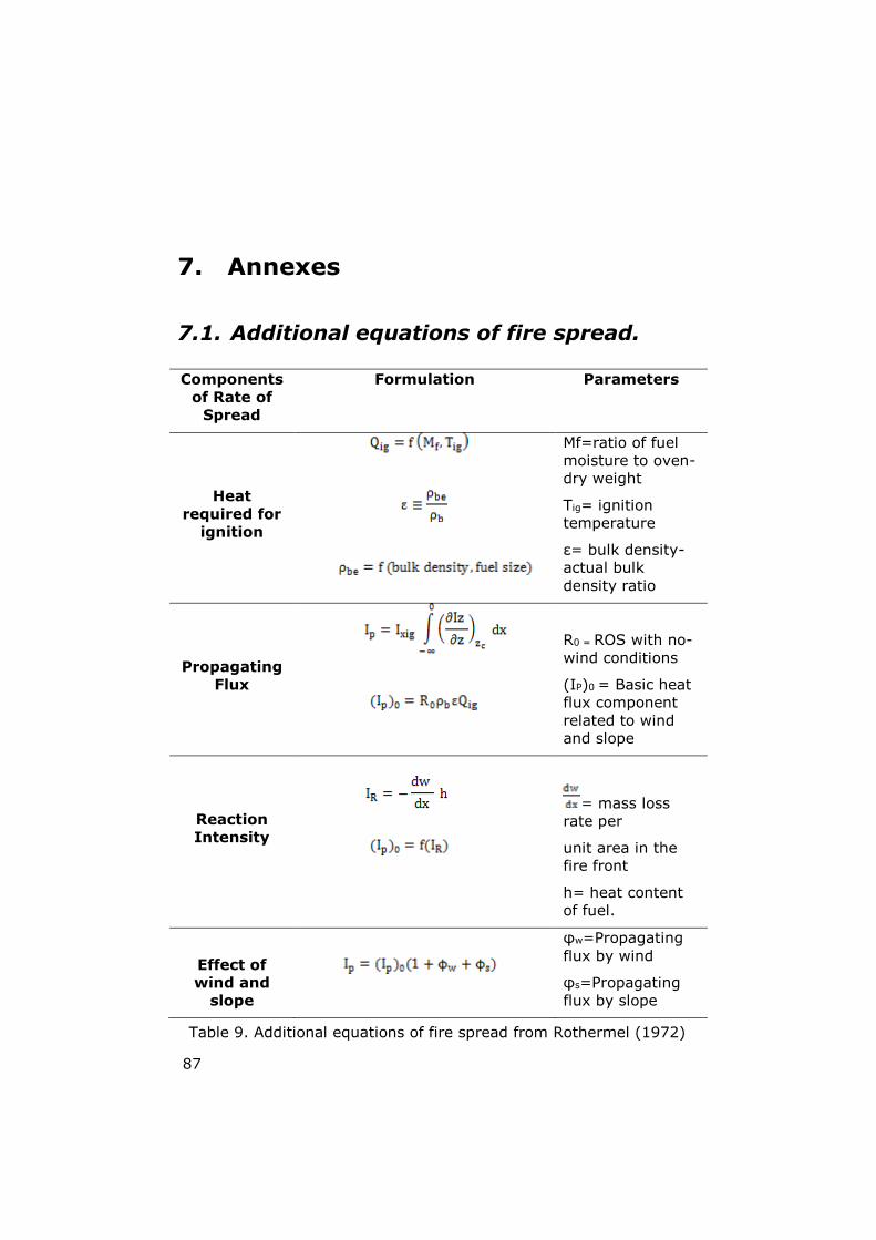
87
7. Annexes
7.1. Additional equations of fire spread.
Components
of Rate of
Spread
Formulation Parameters
Heat
required for
ignition
Mf=ratio of fuel
moisture to oven-
dry weight
Tig= ignition
temperature
ε= bulk density-
actual bulk
density ratio
Propagating
Flux
R0 = ROS with no-
wind conditions
(IP)0 = Basic heat
flux component
related to wind
and slope
Reaction
Intensity
= mass loss
rate per
unit area in the
fire front
h= heat content
of fuel.
Effect of
wind and
slope
φw=Propagating
flux by wind
φs=Propagating
flux by slope
Table 9. Additional equations of fire spread from Rothermel (1972)

Annexes
88
7.2. Additional formulation describing elliptic spread’s shape.
1.
Homogenous
conditions
Formulation Parameters
Without
wind
x, y = coordinates
in plane of a point
in front of the fire
a= rate of spread
t= time elapsed
since ignition.
χ=angular
coordinate which
determine location
of front fire
Constant
wind
f, g & h= wind’s
functions
aft & aht= semi-
axes of the ellipse
ag= Speed of
ellipse’s centre at x-
direction
Table 10. Additional formulation of wind effect from Anderson (1982)
2.
Figure 21. Huygens´ principle
for a steady wind (V)

Chapter 7
89
Table
11.
Main
chara
cte
ristics o
f th
e f
uel ty
pes in lim
esto
ne-d
erived s
oils.
Pro
vence a
rea
Table
12.
Main
chara
cte
ristics o
f th
e f
uel ty
pes in a
cid
ic-d
erived s
oils.
Pro
vence a
rea
7.3. Main characteristics of the fuel types for the Provence region (Curt et al. 2013).
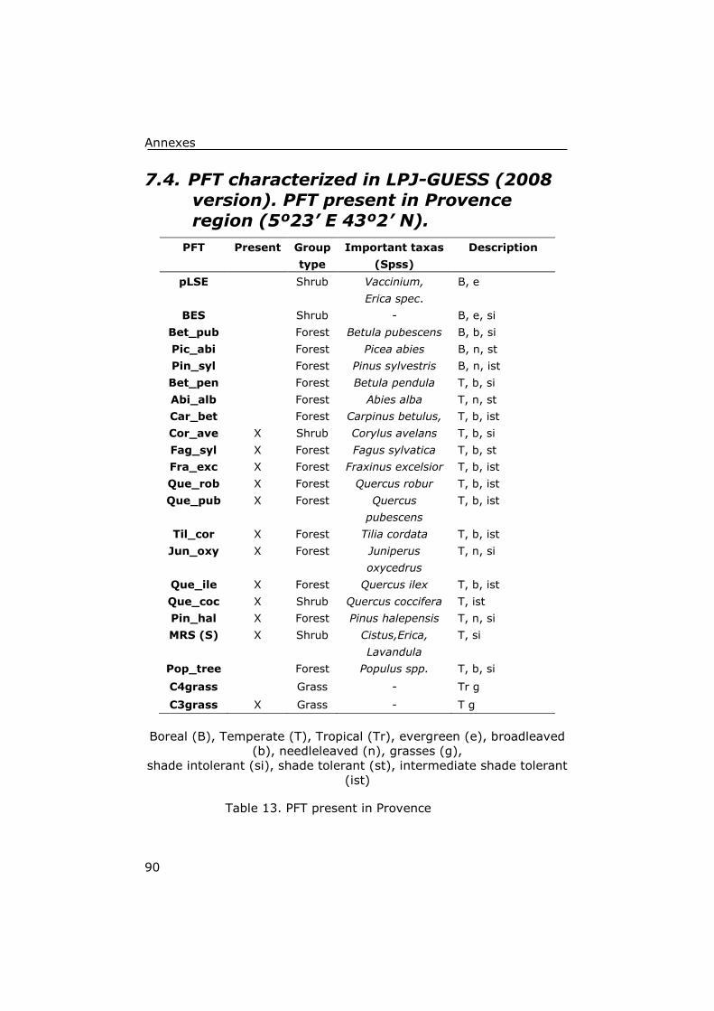
Annexes
90
7.4. PFT characterized in LPJ-GUESS (2008 version). PFT present in Provence region (5º23’ E 43º2’ N).
Boreal (B), Temperate (T), Tropical (Tr), evergreen (e), broadleaved
(b), needleleaved (n), grasses (g),
shade intolerant (si), shade tolerant (st), intermediate shade tolerant
(ist)
PFT Present Group
type
Important taxas
(Spss)
Description
pLSE Shrub Vaccinium,
Erica spec.
B, e
BES Shrub - B, e, si
Bet_pub Forest Betula pubescens B, b, si
Pic_abi Forest Picea abies B, n, st
Pin_syl Forest Pinus sylvestris B, n, ist
Bet_pen Forest Betula pendula T, b, si
Abi_alb Forest Abies alba T, n, st
Car_bet Forest Carpinus betulus, T, b, ist
Cor_ave X Shrub Corylus avelans T, b, si
Fag_syl X Forest Fagus sylvatica T, b, st
Fra_exc X Forest Fraxinus excelsior T, b, ist
Que_rob X Forest Quercus robur T, b, ist
Que_pub X Forest Quercus
pubescens
T, b, ist
Til_cor X Forest Tilia cordata T, b, ist
Jun_oxy X Forest Juniperus
oxycedrus
T, n, si
Que_ile X Forest Quercus ilex T, b, ist
Que_coc X Shrub Quercus coccifera T, ist
Pin_hal X Forest Pinus halepensis T, n, si
MRS (S) X Shrub Cistus,Erica,
Lavandula
T, si
Pop_tree Forest Populus spp. T, b, si
C4grass Grass - Tr g
C3grass X Grass - T g
Table 13. PFT present in Provence

Chapter 7
91
7.5. Input data requirements for FARSITE v4.1.
Input parameter
Range & (metric) Units
File format
File extension
Requisite
Elevation m .ascii .LCP Required
Slope degrees .ascii .LCP Required
Aspect 1-25 .ascii .LCP Required
Fuel model From 1 to 219 .ascii .LCP Required
Canopy cover 0-100 % .ascii .LCP Required
Stand height m (or m*10) .ascii .LCP Optional
Crown base height
m (or m*10) .ascii .LCP Optional
Crown bulk density
Kg/ m3 .ascii .LCP Optional
Duff loading T/ha .ascii .LCP Optional
Coarse Woody Coarse woody models
.ascii .LCP Optional
Adjustments % .txt .ADJ Required
Initial fuel moisture
.txt .CNV Required
Fuel model 1h 0-100% .txt Required
Fuel model 10h
0-100% .txt Required
Fuel model 100h
0-100% .txt Required
LiveH 0-100% .txt Required
LiveW 0-100% .txt Required
Custom Fuel Models
.txt .FMD Optional
Fuel model number
14-89 .txt Optional
Fuel model
code
up to 7 characters .txt Optional
Fuel loading 1h
T/ha .txt Optional
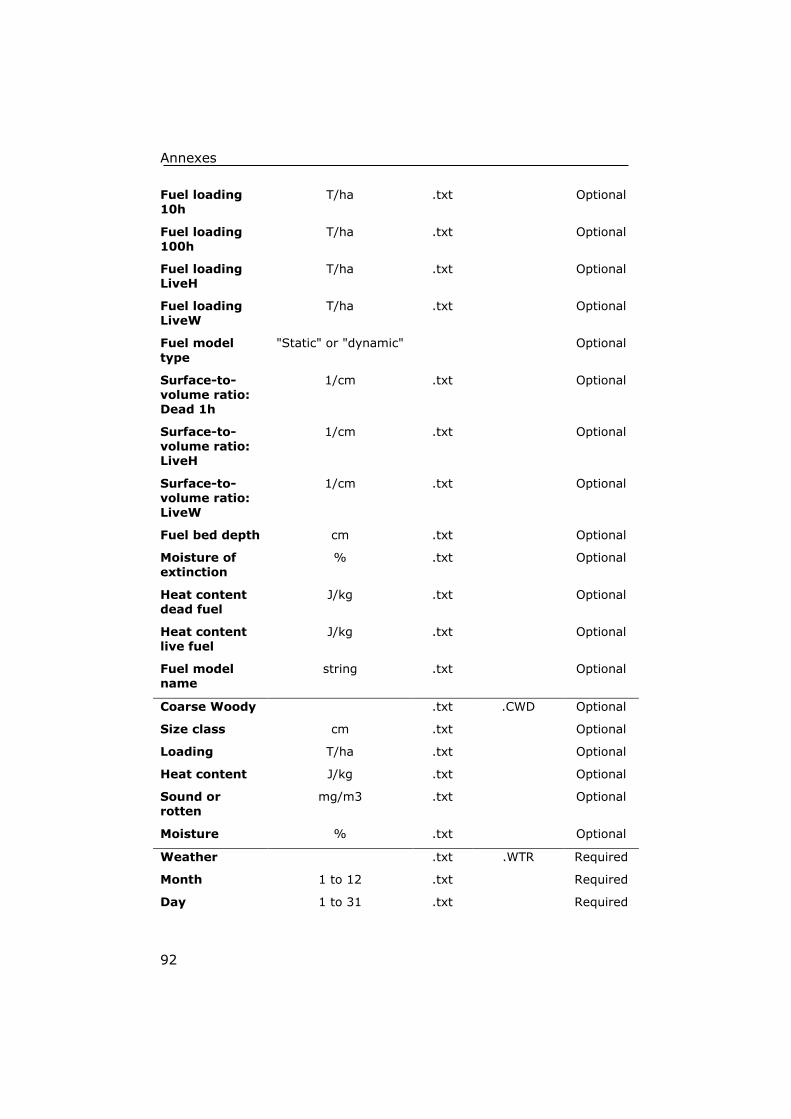
Annexes
92
Fuel loading 10h
T/ha .txt Optional
Fuel loading 100h
T/ha .txt Optional
Fuel loading LiveH
T/ha .txt Optional
Fuel loading LiveW
T/ha .txt Optional
Fuel model
type
"Static" or "dynamic" Optional
Surface-to-volume ratio: Dead 1h
1/cm .txt Optional
Surface-to-volume ratio: LiveH
1/cm .txt Optional
Surface-to-volume ratio: LiveW
1/cm .txt Optional
Fuel bed depth cm .txt Optional
Moisture of extinction
% .txt Optional
Heat content dead fuel
J/kg .txt Optional
Heat content live fuel
J/kg .txt Optional
Fuel model name
string .txt Optional
Coarse Woody .txt .CWD Optional
Size class cm .txt Optional
Loading T/ha .txt Optional
Heat content J/kg .txt Optional
Sound or rotten
mg/m3 .txt Optional
Moisture % .txt Optional
Weather .txt .WTR Required
Month 1 to 12 .txt Required
Day 1 to 31 .txt Required

Chapter 7
93
Daily precipitation
mm .txt Required
Hour of minimum temperature
0-2400 hr txt Required
Hour of maximum temperature
0-2400 hr .txt Required
Minimum
temperature
°Celsius .txt Required
Maximum temperature
°Celsius .txt Required
Minimum humidity
0-99 % .txt Required
Maximum humidity
0-99 % .txt Required
Elevation m .txt Required
Precipitation duration: rt1 & rt2
0-2400 hr .txt Optional
Wind .txt .WND Required
Hour 0-2359 hr .txt Required
Speed (10 m) 0-300 km/h .txt Required
Direction 0-360° .txt Required
CloudCover 0-100 % .txt Required
Burn period .txt .CRW Optional
Month 1 to 12 .txt Optional
Day 1 to 31 .txt Optional
StartHour 0-2400 hr .txt Optional
EndHour 0-2400 hr .txt Optional
Table 14. Input data requirements in FARSITE

94
7.6. Variable selection from LPJ-GUESS-SPITFIRE to FARSITE.
Output parameter
LPJ-GUESS
Units Input parameter
FARSITE
Units
Custom
Fuel
Model
fuel_1hr_total gDM C/m2 ←→ Fuel loading 1h T/ha
fuel_10hr_total gDM C/m2 ←→ Fuel loading 10h T/ha
fuel_100hr_total gDM C/m2 ←→ Fuel loading 100h T/ha
livegrass gDM /m2 ←→ Fuel loading LiveH T/ha
fuel_1000hr_total g C/m2 ←→ Fuel loading LiveW T/ha
lm g/m2 ←→
sm g/m2 ←→
hm g/m2 ←→
rm g/m2
sigma_1hr 66 cm−1 ←→ SAV ratio: Dead 1h 1/cm
sigma_10hr 3.58 cm−1 SAV ratio: Dead 10h 1/cm
sigma_100hr 0.98 cm−1 SAV ratio: Dead 100h 1/cm
sigma_grass 80 cm−1 ←→ SAV ratio: LiveW 1/cm
sigma_1000hr 0.5 cm−1 ←→ SAV ratio: LiveH 1/cm

Chapter 7
95
Custom
Fuel
Model
Litterme (grass) 0.2 ←→ Moisture of extinction %
Litterme (shrub) 0.3 ←→ Moisture of extinction %
Litterme (tree) 0.3 ←→ Moisture of extinction %
H 18 000 KJ/Kg ←→ Heat content dead fuel KJ/kg
Fuel depth m ←→ Fuel depth m
Coarse woody model
steam diamer cm ←→ Size class cm
←→ Loading T/ha
←→ Sound or rotten mg/m3
←→ Moisture %
Tree
para-meters
fpc_tree % ←→ Canopy cover %
height*crown_l m ←→ Stand height m
crown_l m ←→ Crown base height m
←→ Crown bulk density Kg/ m3
Fuel moisture
dlm_1 ←→ Fuel model 1h 0-100%
dlm_10 ←→ Fuel model 10h 0-100%
dlm_100 ←→ Fuel model 100h 0-100%
dlm_lg ←→ LiveH 0-100%
←→ LiveW 0-100%
Table 15. Variable selection from LPJ-GUESS-SPITFIRE

96
7.7. LPJ-GUESS-SPITFIRE code’s implementation
1.
if (date.islastday && date.islastmonth) {
// LAST DAY OF YEAR
// Call input/output
module to output results for end of year
// or end of simulation for this grid cell
outannual(gridcell,pftlist);
if(date.year>1000)
{
printf("year %d \n", date.year);
}
// Check whether to abort
if (abort_request_received()) {
termio();
return 99;
}
}
2.
// crown_base_height: simple multiplication between tree
height and crown length proportion
fire_ind[indinummer].crown_base_height=(indiv.height)*(pftli
st[indiv.pft.id].crown_l);
// fuel_depth: dead load fuel (1h+10h+100h) divided by the
fuel's density
fuel_depth=dead_fuel/char_dens_fuel_ave;

Chapter 7
97
// Following the same structure used by Thonicke et al. (2010)
for fuel moisture calculation (composite //estimate of moisture
content for 1h, 10h, 100h fuels), I decided to split the
calculation for each //specific fuel class: dlm_1hr, dlm_10hr,
dlm_100hr:
dlm_1hr=exp(-(alpha_1hr*fuel_1hr_total)*ni_acc[date.day]);
dlm_10hr=exp(-(alpha_10hr*fuel_10hr_total)*
ni_acc[date.day]);
dlm_100hr=exp(-(alpha_100hr*fuel_100hr_total)*
ni_acc[date.day]);
// Fire behaviour described by Andrews (1986)
flame_residence_time=12.595/sigma;
flame_length=0.047* pow (d_i_surface,0.46);
heat_per_unit_area=ir*flame_residence_time;
3.
//Canopy cover
printf("fpc grass %f % \n",fpc_grass_total);
//Tree parameters (no individual calculation)
printf("dbh %f cm \n",fire_ind->dbh,);
printf("height %f m \n",fire_ind->height);
printf("crown_base_height %f m \n",fire_ind-
>crown_base_height); printf("crown_l %f % \n",fire_ind->crown_length,);
// Dead fuel loading
printf("dead_fuel_sum %f gCDM/m2 \n",dead_fuel); // total fuel loading
printf("fuel_1hr_total %f gCDM/m2 \n",fuel_1hr_total);// 1h
printf("fuel_10hr_total %f gCDM/m2 \n",fuel_10hr_total);//
10h
printf("fuel_100hr_total %f gCDM/m2
\n",fuel_100hr_total);// 100h
printf("fuel_1000hr_total %f gCDM/m2
\n",fuel_1000hr_total);// 1000h printf("fuel_grass %f gC/m2 \n",livegrass);// living grass

Annexes
98
// Living fuel loading (Sum of individuals?)
printf("leaf_mass %f g/m2 \n",fire_ind->lm);// Living leaf
mass
printf("sapwood_mass %f g/m2 \n",fire_ind->sm);Living
sapwood mass
printf("heartwood_mass %f \n",fire_ind->hm,"g/m2");Living heartwood mass
//Fuel depth printf("fuel_depth %f cm \n",fuel_depth);
// Moisture-related printf("Mx %f \n",char_moistfactor);
// Moisture of extinction
printf("ni_acc %f \n",ni_acc[date.day]);// Nesterov Index
printf("dlm_deadfuel %f \n",dlm);// Composite estimation
moisture
printf("dlm_1h %f \n",dlm_1hr);// 1h fuel moisture
printf("dlm_10h %f \n",dlm_10hr);// 10h fuel moisture
printf("dlm_100h %f \n",dlm_100hr);// 100h fuel moisture printf("dlm_lg %f \n",dlm_lg);// living grass fuel moisture
4.
//Change loop’s location allowing computation even during NO-FIRE
year's event. It is placed after calculation //of the variables
if (ifdespitefire &&
has_not_burned_last_six_month
&& //only
perform calculation if patch has not already burned in the last six
months
(
(fixrandfirereturninterval>-
0.5 && date.day==fixburnday-1) ||
// if fixrandfire is set only at the day when it burns
(fixfirereturninterval>-0.5 &&
date.day==fixburnday-1 && date.year %int
(fixfirereturninterval)==0.) ||
// if fixfire is
set only at the day when it burns
(readinburnarea &&
climate.fire_io.baprob>0) ||
// if burned area read is set, only to

Chapter 7
99
do if the probability (ba) within the reading //
file is above 0
statisticburnarea ||
ifdefafnd ||
burnyear ==
date.year
)
)
{
5.
//////////////FIRE BEHAVIOUR PFT SPECIFIC
for(int pft=0;pft<npft;pft++){
beta_pft[pft]=char_dens_fuel_ave_pft[pft]/part_dens;
beta_opt_pft[pft]=0.20395*(pow(sigma_pft[pft],-0.8189)); //FIX
//beta_opt_pft[pft]=0.200395*(pow(sigma_pft[pft],-0.8189));
bet_pft[pft]=beta_pft[pft]/beta_opt_pft[pft];
//////////////////////////////////////////////////heat of pre ignition
q_ig_pft[pft]=581+2594*dlm_pft[pft]; // FIX
//q_ig_pft[pft]=581+94*dlm_pft[pft];
//////////////////////////////////////////////////effective heating number
eps_pft[pft]=exp(-4.528/sigma_pft[pft]);
//////////////////////////////////////////////////influence of wind speed
a_pft[pft]=8.9033*pow(sigma_pft[pft],-0.7913);
//b_pft[pft]=0.15988*pow(sigma_pft[pft],0.55); //FIX
b_pft[pft]=0.15988*pow(sigma_pft[pft],0.54);
c_pft[pft]=7.47*(exp(-0.8711*pow(sigma_pft[pft],0.55)));
e_pft[pft]=0.715*(exp(-0.01094*sigma_pft[pft]));
phi_wind_pft[pft]=c_pft[pft]*(pow(wind_forward_pft[pft],b_pft[pft])
)*pow(bet_pft[pft],-e_pft[pft]); // was base_wind before
////////////////////////////////////////////////////////////propagating
flux M_16
if (sigma_pft[pft]<0.00001)
xi_pft[pft]=0.;
else
{
xi_pft[pft]=(exp((0.792+3.7597*pow(sigma_pft[pft],0.5))*(beta_pf
t[pft]+0.1)))/(192+7.9095*sigma_pft[pft]);
}
////////////////////////////////////////////////////////////reaction
intensity M_17
if (sigma_pft[pft]<=0.00001)

Annexes
100
dummy_pft[pft]=0.;
else
dummy_pft[pft]=exp(a_pft[pft]*(1-bet_pft[pft]));
gamma_max_pft[pft]=1/(0.0591+2.926*pow(sigma_pft[pft],-1.5));
gamma_aptr_pft[pft]=gamma_max_pft[pft]*pow(bet_pft[pft],a_pft[
pft])*dummy_pft[pft];
if (char_moistfactor_pft[pft]>0.)
mw_weight_pft[pft]=dlm_pft[pft]/char_moistfactor_pft[pft];
else
mw_weight_pft[pft]=0.;
moist_damp_pft[pft]=max(0.,(1-
(2.59*mw_weight_pft[pft])+(5.11*(mw_weight_pft[pft]*mw_weight
_pft[pft]))-(3.52*pow(mw_weight_pft[pft],3))));
ir_pft[pft]=gamma_aptr_pft[pft]*char_net_fuel_pft[pft]*H*moist_da
mp_pft[pft]*MINER_DAMP;
if (((char_dens_fuel_ave_pft[pft]<=0.) | (eps_pft[pft]<=0.) |
(q_ig_pft[pft]<=0.) |(ir_pft[pft]<=0. )))
u_front_pft[pft]=0.;
else
u_front_pft[pft]=(ir_pft[pft]*xi_pft[pft]*(1.0+phi_wind_pft[pft]))/(ch
ar_dens_fuel_ave_pft[pft]*eps_pft[pft]*q_ig_pft[pft]); // ROS
ros_f_pft[pft]=u_front_pft[pft];
////////////////////////////////////////////////////////////////////Backwar
d spread
ros_b_pft[pft]=ros_f_pft[pft]*exp(-0.012*wind_speed_pft[pft]);
////////////////////////////////////////////////////////////////////fire
duration M_19
if (ros_b_pft[pft]<0.05 ) //0.05
ros_b_pft[pft]=0.;
fire_durat_pft[pft]=241/(1+(((240))*exp(-11.06*d_fdi_pft[pft])));
db_pft[pft]=ros_b_pft[pft]*fire_durat_pft[pft];
df_pft[pft]=ros_f_pft[pft]*fire_durat_pft[pft]; //}
if (net_fuel_pft[pft]<=0.) {
ros_b_pft[pft]=0.;
db_pft[pft]=0.;
ros_f_pft[pft]=0.;
df_pft[pft]=0.;
}
if (date.year==1025 && date.day==212)
{
printf(" pft %d year %d date %d ROS %f ROStot %f Ir %f Irtot %f
\n", pft,date.year,date.day,ros_f_pft[pft],ros_f,ir_pft[pft],ir);
}
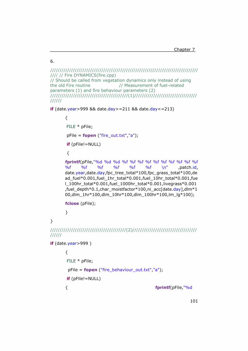
Chapter 7
101
6.
//////////////////////////////////////////////////////////////////////////////
//// // Fire DYNAMICS(fire.cpp)
// Should be called from vegetation dynamics only instead of using
the old Fire routine // Measurement of fuel-related
parameters (1) and fire behaviour parameters (2)
/////////////////////////////////////////(1)///////////////////////////////////////
if (date.year>999 && date.day>=211 && date.day<=213)
{
FILE * pFile;
pFile = fopen ("fire_out.txt","a");
if (pFile!=NULL)
{
fprintf(pFile,"%d %d %d %f %f %f %f %f %f %f %f %f %f
%f %f %f %f %f %f \n" ,patch.id,
date.year,date.day,fpc_tree_total*100,fpc_grass_total*100,de
ad_fuel*0.001,fuel_1hr_total*0.001,fuel_10hr_total*0.001,fue
l_100hr_total*0.001,fuel_1000hr_total*0.001,livegrass*0.001
,fuel_depth*0.1,char_moistfactor*100,ni_acc[date.day],dlm*1
00,dlm_1hr*100,dlm_10hr*100,dlm_100hr*100,lm_lg*100);
fclose (pFile);
}
}
////////////////////////////////////////(2)////////////////////////////////////////
if (date.year>999 )
{
FILE * pFile;
pFile = fopen ("fire_behaviour_out.txt","a");
if (pFile!=NULL)
{ fprintf(pFile,"%d

Annexes
102
%d %d %f %f %f %f %f %f %f %f %f %f %f %f %f %f %f
%f %f %f %f %f \n" ,patch.id,
date.year,date.day,ir,xi,phi_wind,beta,eps,q_ig,ROS_f,ROS_b,
bet,
beta_opt,fire_durat,db,df,d,numfire,d_fdi,fire_frac,area,flame_
residence_time,flame_length,heat_per_area);
fclose (pFile);
}
}
//////////////////////////////////////////////////////////////////////////////
//////TREE ALLOMETRY (growth.cpp)
//Should be called to update allometry, FPC and FPC increment
whenever biomass values for a vegetation //individual change.
Calculates tree allometry (height and crown area) and fractional
projective given carbon //biomass in various compartments for an
individual.
///////////////////////////////////////////////////////////////////////////////////////
if (date.year>999)
{
FILE * pFile;
pFile = fopen ("tree_out.txt","a");
if (pFile!=NULL)
{
fprintf(pFile, "%d %d %d %d %f %f %f %f %f %f \n"
,nr_of_patch,date.year,date.month, date.day,indiv.height,
indiv.pft.crown_l,indiv.cmass_leaf,
,indiv.cmass_sap,indiv.cmass_heart, vol );
fclose (pFile);
}
}

Chapter 7
103
7.8. LPJ-GUESS-SPITFIRE code’s modification
1.
//Start of calculations based on Rothermel's equations
beta=char_dens_fuel_ave/part_dens;
beta_opt=0.20395*(pow(sigma,-0.8189)); // Instead of
beta_opt=0.200395*(pow(sigma,-0.8189));
bet=beta/beta_opt;
//////////////////////////////////////////////////heat of pre ignition
q_ig=581+2594*dlm; // Instead of q_ig=581+94*dlm
2.
// Area calculation in m2
area=(12321200000*cos(climate.lat*0.017453280))*pixeldegree*pix
eldegree;
// instead of
area=(1232120000*cos(climate.lat*0.017453280))*pixeldegree*pixe
ldegree

Annexes
104
7.9. Synthetic landscape’s creation from LPJ-GUESS-SPITFIRE through MATLAB code
%%% Importation from .txt file computed in LPJ-GUESS-SPITFIRE.
Canopy cover, tree height, crown height and fuel follow the same
structure. An example of CC is shown%%%
clear, clf format short % Importing output data from LPJ-GUESS-SPITFIRE load CC.txt % Creating 1000000 m2 synthetic landscape ((10x10)*100) !patch(1:100)=1:100; mapmatrix= zeros(100,10); for patchi=1:100, for cellxi=1:10, for cellyi=1:10, mapmatrix(mod(patchi-
1,10)*10+cellxi,ceil(patchi/10)*10+cellyi)=CC(patchi); ,end,end,end; xlswrite('CC.xls',mapmatrix) % Creating 10000 m2 synthetic landscape (10x10) mapmatrix1= zeros(10,10); for i=1:10; for j=1:10; mapmatrix1(i,j)= mapmatrix(i+(i-1)*10,j*10+1); end end imagesc(mapmatrix1); xlswrite('CC1.xls',mapmatrix1)

105
Figure 22. Canopy cover, fuel depth, Mx, fuel loading and fuel moisture mean values over 30 years' time series
7.10. Fuel-related variables in a 30 years’ time series

Annexes
106
7.11. Synthetic landscape based on 9 patch custom fuel model
Table X. Syntetic landscape based on 9 patch custom fuel model
Fuel
Model
Depth
(cm)Mx (%)
1h 10h 100h live 1h 10h 100h H W
p14 3.08 1.01 3.63 2.57 77.13 30 2 2 2 5.00 100.00
p15 2.34 0.01 0.03 2.57 23.79 29.45 2 75.71 40.84 5.00 100.00
p16 2.18 0.03 0.09 2.57 22.93 29.96 2 39.33 4.96 5.00 100.00
p24 2.77 0 0 2.57 27.68 28.19 2 99.99 99.96 5.00 100.00
p25 2.47 1.04 3.74 2.57 72.44 29.99 2 2 2 5.00 100.00
p26 2.8 1.17 4.2 2.57 81.64 29.92 2 2 2 5.00 100.00
p34 3.08 0.04 0.13 2.57 32.52 29.79 2 26.32 2 5.00 100.00
p35 3.35 0.9 3.23 2.57 74.71 29.58 2 2 2 5.00 100.00
p36 2.92 0 0 2.57 29.24 29.71 2 99.96 99.87 5.00 100.00
* Heat content=18600 kJ/Kg for all fuel models
Fuel load (t.ha-1) Initial DFMC (%) LFMC (%)
Table 16. Custom
fuel model of 9
patches
Figure 10. Boxplots:
LPJ-GUESS-FARSITE
simulations based on
9 custom fuel models

Chapter 7
107
Date
Plant
height
(m)
Dominate Spp
Max
temp
(°C)
Min
temp
(°C)
Mean
temp
Relative
humidity
(%)
Wind
speed
(km/h)
Wind
direction
(°)
Observe
d
(m/min)
Simulate
d
(m/min)
Location A
Augus
t 26,
2004
1.0-4.0
Pistacia lentiscus
L. Olea europaca L.
var. oleaster,
Cistus
monpeliensisL.,
Myrtus communis
L.
28 20 - - 35
western-
south-
western
8.1 8.1
Location B
Augus
t 21,
2004
-
Pistacia lentiscus
L., Arbutus Unedo
L., Olea europaca
L. var. oleaster,
Cistus spp., Myrtus
communis L.
- - 24 35 15 280 2.8 3
Location C
Augus
t 11,
2004
1.5-2.0
Pistacia lentiscus
L., Arbutus Unedo
L., Olea europaca
L. var. oleaster,
Cistus spp., Myrtus
communis L.
39 25 - - 13 295 13 13
Location
D
July
15,
2006
1.0-1.5
Pistacia lentiscus
L., Arbutus Unedo
L., Myrtus
communis L, grass
36 20 - - 11 40 4.6 4.6
ROS Conditions
7.12. Observed vs simulated ROS measurements in Sardinia, Italy (Salis 2007).
Table 17. Observed vs Simulated ROS

108
7.13. Examples of fire behaviour. From Albini F.A unpublished training notes (Pyne et al. (1996)
ROS (m/min) Typical fire situation Equivalent to
0.31 Litter fire, no wind no slope
Line building rate for one person in heavy fuel
7.62 Aged medium slash, 100% slope
Backpacker going up 100% slope
76.2 Low sagebrush, Santa Ana wind
Brisk walk on level ground
243.8 Chaparral, Santa Ana wind
Good pace for a marathon run
365,8 Dry, short grass, strong
wind
4-minute mile
Table 18. Examples of Rate of Spread
IR (kW/m2) Fuel consumed (T/ha)
Energy released on 0.61 m2 would…
56.78 1.9 (grass) Warm up 2 quarts of stew
227.11 7.4 (tall grass) Boil away 1 pint of water 757.06 24.7 (2.5 cm. pine
duff) Open car thermostat
2271.18 74.1 (thinning slash) Heat 10 Pulaski heads to full cherry red
9084.74 296.5(heavy logging
debris)
Melt down an aluminium engine
block (52 kg)
Table 19. Examples of Reaction intensity
FML (m) FLI (Kj/m/s) Fire suppression interpretation
< 1.2 <346.1 Fire can generally be attacked at the head or flanks
1,2 – 2.4 346.1-1730.6 Fires are too intense for direct attack on the head
2.4- 3.4 1730.6-3461.3 Fires may present serious control problems: torching, crowing and
spotting. Control efforts at fire head will probably be ineffective
>3.4 >3461.3 Crowing and spotting and major fire runs are probable. Control efforts at
fire head are ineffective
Table 20. Flame length and Fire-line intensity related to fire
suppression activities

Chapter 7
109
7.14. Scripts used in digital format.
Due to the large extension of each of the implementations, and the
new routine created along the original code, a full copy of the
modified code has been enclosed in digital format instead. The CD
enclosed to the MSc thesis includes 3 folders containing:
1. LPJ-GUESS-SPITFIRE:
-Folder “eclipse_proj_fire”: the guess_ins.txt and gridlist.txt
used.
-Folder “fire” and sub-folder “modules”: the altered versions of
the codes. Major changes are presented in fire.cpp and
growth.cpp module.
2. R:
-All the scripts involving the visualization of histograms and
boxplots together with the statistical tests performed are in
COMPARISON ANALYSIS.R.
-Row data used for each theme.
3. MATLAB:
-The script in charge of the synthetic landscape generation is
written in Metamodel_m.
-Row data (Canopy cover, tree height, crown height and fuel)
for each map creation.

Annexes
110
111
8. List of references
Acácio, V., M. Holmgren, F. Rego, F. Moreira, and G. M. J. Mohren. 2009. Are drought and wildfires turning Mediterranean cork oak forests into persistent shrublands? Agroforestry Systems, 76: 389-400. DOI: 10.1007/s10457-008-9165-y
Albini, F. A., 1976a. Estimating Wildfire Behaviour and Effects. Intermountain Forest and Range Experiment Station, Forest Service, U.S. Department of Agriculture General Technical Report INT-30, Ogden, Utah, USDA Forest Service 100 pp.
Albini, F. A., 1979. Spot Fire Distance from Burning Trees: A Predictive Model. Intermountain Forest and Range Experiment Station, Forest Service, U.S. Department of Agriculture General Technical Report INT-56, Ogden, Utah, USDA Forest Service 80 pp.
Albini, F. A., and E. D. Reinhardt. 1995. Modeling ignition and burning rate of large woody natural fuels. International Journal of Wildland Fire, 5(2): 81-91.
Alexander, M. E., and M. G. Cruz. 2012. Interdependencies between flame length and fireline intensity in predicting crown fire initiation and crown scorch height. International Journal of Wildland Fire, 21: 95-113. DOI: http://dx.doi.org/10.1071/WF11001
Anderson, D. H., E. A. Catchpole, N. J. De Mestre, and T. Parkes. 1982. Modelling the spread of grass fires. The ANZIAM Journal, 23: 451-466. DOI: doi:10.1017/S0334270000000394
Anderson, H. E., 1969. Heat Transfer and Fire Spread. Intermountain Forest and Range Experiment Station, Forest Service, U.S. Department of Agriculture Research Paper INT-69, Ogden, Utah, USDA Forest Service 29 pp.
Anderson, H. E., 1982. Aids to Determining Fuel Models for Estimating Fire Behavior. Intermountain Forest and Range Experiment Station, Forest Service, U.S. Department of Agriculture General Technical Report INT-122, Ogden, Utah, USDA Forest Service 28 pp.
Andrews, P. L., 1986. BEHAVE: Fire Behavior Prediction and Fuel Modeling System - BURN Subsystem, Part 1. Intermountain Forest and Range Experiment Station, Forest Service, U.S.
List of references
112
Department of Agriculture General Technical Report INT-194, Ogden, Utah, USDA Forest Service 134 pp.
Arca, B., P. Duce, M. Laconi, G. Pellizzaro, M. Salis, and D. Spano. 2007. Evaluation of FARSITE simulator in Mediterranean maquis. International Journal of Wildland Fire, 16: 563-572. DOI: http://dx.doi.org/10.1071/WF06070
Arca, B., M. Laconi, A. Maccioni, G. Pellizzaro, and M. Salis. 2005. Validation of Farsite Model in Mediterranean Area. 4. University of Sassari.
Archibald, S., A. Nickless, N. Govender, R. J. Scholes, and V. Lehsten. 2010. Climate and the inter-annual variability of fire in southern Africa: a meta-analysis using long-term field data and satellite-derived burnt area data. Global Ecology and Biogeography, 19: 794-809. DOI: 10.1111/j.1466-8238.2010.00568.x
Arora, V. K., and G. J. Boer. 2005. Fire as an interactive component of dynamic vegetation models. Journal of Geophysical Research-Biogeosciences, 110. DOI: 10.1029/2005jg000042
Barrows, J. S., 1951. Fire Behavior in Northern Rocky Mountain Forests. Northern Rooky Mountain Forest and Range Experiment Station, Forest Service, U.S. Department of Agriculture Station Paper No. 29, Missoua, Montana, USDA Forest Service 134 pp.
Bowman, D., J. K. Balch, P. Artaxo, W. J. Bond, J. M. Carlson, M. A. Cochrane, C. M. D'Antonio, R. S. DeFries, et al. 2009. Fire in the Earth System. Science, 324: 481-484. DOI: 10.1126/science.1163886
Byram, G. M. 1959. Combustion of Forest Fuels. In: Davis, K. P. Forest Fire: Control and Use, 61-89 pp. New York: McGraw-Hill Book Company.
Canellas, I., and A. S. Miguel. 1998. Litter fall and nutrient turnover in Kermes oak (Quercus coccifera L.) shrublands in Valencia (eastern Spain). Annales Des Sciences Forestieres, 55: 589-597. DOI: 10.1051/forest:19980506
Caritat, A., E. García-Berthou, R. Lapeña, and L. Vilar. 2006. Litter production in a Quercus suber forest of Montseny (NE Spain) and its relationship to meteorological conditions. Ann. For. Sci., 63: 791-800. DOI: http://dx.doi.org/10.1051/forest:2006061
Castells, E., J. Peñuelas, and D. W. Valentine. 2004. Are phenolic compounds released from the Mediterranean shrub Cistus
Chapter 8
113
albidus responsible for changes in N cycling in siliceous and calcareous soils? New Phytologist, 162: 187-195. DOI: 10.1111/j.1469-8137.2004.01021.x
Chandler, C., P. Cheney, P. Thomas, L. Trabaud, and D. Williams. 1983. Fire in forestry. Volume 1. Forest fire behavior and effects. New York: John Wiley & Sons, Inc.
Cheney, N. P., and J. S. Gould. 1995. Fire Growth in Grassland Fuels. International Journal of Wildland Fire, 5: 237-247. DOI: http://dx.doi.org/10.1071/WF9950237
Cohen, J. D., and J. E. Deeming, 1985. The National Fire-Danger Rating System: basic equations. Pacific Southwest Forest and Range Experiment Station, Forest Service, U.S. Department of Agriculture General Technical Report PSW-82, Berkeley, California, USDA Forest Service, 23 pp.
Cramer, W., A. Bondeau, F. I. Woodward, I. C. Prentice, R. A. Betts, V. Brovkin, P. M. Cox, V. Fisher, et al. 2001. Global response of terrestrial ecosystem structure and function to CO2 and climate change: results from six dynamic global vegetation models. Global Change Biology, 7: 357-373. DOI: 10.1046/j.1365-2486.2001.00383.x
Curt, T., W. Adra, and L. Borgniet. 2009. Fire-driven oak regeneration in French Mediterranean ecosystems. Forest Ecology and Management, 258: 2127-2135. DOI: 10.1016/j.foreco.2009.08.010
Curt, T., L. Borgniet, and C. Bouillon. 2013. Wildfire frequency varies with the size and shape of fuel types in southeastern France: Implications for environmental management. Journal of Environmental Management, 117: 150-161. DOI: 10.1016/j.jenvman.2012.12.006
Curt, T., A. Schaffhauser, L. Borgniet, C. Dumas, R. Esteve, A. Ganteaume, M. Jappiot, W. Martin, et al. 2011. Litter flammability in oak woodlands and shrublands of southeastern France. Forest Ecology and Management, 261: 2214-2222. DOI: 10.1016/j.foreco.2010.12.002
Curt, T., A. Schaffhauser, L. Borgniet, R. Esteve, A. Ganteaume, M. Jappiot, C. Lampin-Maillet, W. Martin, et al. 2010. Litter flammability of French Mediterranean vegetation types: a cross-substratum analysis. In VI International Conference on Forest Fire Research ed. D. X. Viegas, 8. Coimbra, Portugal.
Delitti, W., A. Ferran, L. Trabaud, and V. R. Vallejo. 2005. Effects of fire recurrence in Quercus coccifera L. shrublands of the

List of references
114
Valencia Region (Spain): I. plant composition and productivity. Plant Ecology, 177: 57-70. DOI: 10.1007/s11258-005-2140-z
Dopheide, E., F. van der Meer, R. Sliuzas, A. van der Veen, and A. Voinov. 2012. System Earth: some theory on the system. In The core of GIScience: a systems-based approach. Enschede, The Netherlands: The International Institute for Geo-Information Science and Earth Observation (ITC).
Eugenio, M., I. Verkaik, F. Lloret, and J. M. Espelta. 2006. Recruitment and growth decline in Pinus halepensis populations after recurrent wildfires in Catalonia (NE Iberian Peninsula). Forest Ecology and Management, 231: 47-54. DOI: http://dx.doi.org/10.1016/j.foreco.2006.05.007
FCFDG, 1992. Development and Structure of the Canadian Forest Fire Behavior Prediction System. Group Information Report ST-X-3, Ottawa,Forestry Canada Fire Danger
Finney, M. A., 2004. FARSITE: Fire Area Simulator - Model development and evaluation. Rocky Mountain Research Station, Forest Service, U.S. Department of Agriculture. Rearch Paper RMRS-RP-4 (Revised), Fort Collins, CO, USDA Forest Service 52 pp.
Finney, M. A., R. C. Seli, and P. L. Andrews. 2003. Modeling post-frontal combustion in the FARSITE fire area simulator. In Second International Wildland Fire Ecology and Fire Management Congress and Fifth Symposium on Fire and Forest Meteorology, p. 125. Orlando, FL. : American Meteorological Society.
Foley, J. A. 1995. An equilibrium model of the terrestrial carbon budget. Tellus B, 47: 310-319. DOI: 10.1034/j.1600-0889.47.issue3.3.x
Fosberg, M. A., W. Cramer, V. Brovkin, R. Fleming, R. Gardner, A. M. Gill, J. G. Goldammer, R. Keane, et al. 1999. Strategy for a fire module in dynamic global vegetation models. International Journal of Wildland Fire, 9: 79-84. DOI: 10.1071/wf99007
Frandsen, W. H. 1971. Fire spread through porous fuels from the conservation of energy. Combustion and Flame, 16: 9-16. DOI: 10.1016/S0010-2180(71)80005-6
Fujioka, F. M., A. M. Gill, D. X. Viegas, and B. M. Wotton. 2008. Fire Danger and Fire Behavior Modeling Systems in Australia, Europe, and North America. In Wildland Fires and Air Pollution. Developments in Environmental Science, eds. Andrzej Bytnerowicz, M. J. Arbaugh, A. R. Riebau, and A. Christian, 471-497 pp.: Elsevier.

Chapter 8
115
Ganteaume, A., M. Jappiot, C. Lampin-Maillet, T. Curt, and L. Borgniet. 2009. Fuel characterization and effects of wildfire recurrence on vegetation structure on limestone soils in southeastern France. Forest Ecology and Management, 258: S15-S23. DOI: 10.1016/j.foreco.2009.07.021
Ganteaume, A., M. Jappiot, C. Lampin-Maillet, T. Curt, and L. Borgniet. 2011. Effects of vegetation type and fire regime on flammability of undisturbed litter in Southeastern France. Forest Ecology and Management, 261: 2223-2231. DOI: http://dx.doi.org/10.1016/j.foreco.2010.09.046
Gill, A. M. 1979. Fire in the Australian landscape. Landscape Planning, 6: 343-357. DOI: http://dx.doi.org/10.1016/0304-3924(79)90037-6
Gordon, B. B. 2008. Ecological Climatology: Concepts and Applications (2nd Edition). New York: Cambridge University Press.
Hättenschwiler, S., and P. M. Vitousek. 2000. The role of polyphenols in terrestrial ecosystem nutrient cycling. Trends in Ecology & Evolution, 15: 238-243. DOI: http://dx.doi.org/10.1016/S0169-5347(00)01861-9
Houghton, J. T., Y. Ding, D. J. Griggs, N. Noguer, P. J. Van der Linden, D. Xiaosu, K. Maskell, and C. A. Johnson, 2001. Climate change 2001: The scientific basis, Contribution of Working Group I to the Third Assessment Report of the Intergovernmental Panle on Climate Change. Candbridge University Press 1477-870X, New York.
Incerti, G., G. Bonanomi, F. Giannino, F. A. Rutigliano, D. Piermatteo, S. Castaldi, A. De Marco, A. Fierro, et al. 2011. Litter decomposition in Mediterranean ecosystems: Modelling the controlling role of climatic conditions and litter quality. Applied Soil Ecology, 49: 148-157. DOI: http://dx.doi.org/10.1016/j.apsoil.2011.06.004
Johnson, E. A., and K. Miyanishi. 2001. Forest Fires: Behavior and Ecological Effects. Elsevier Science.
JRC-EFFIS. 2012. Forest Fires in Europe, Middle East and North Africa. 118p. Land Management and Natural Hazards Unit.
Lehsten, V. 2013. Vegetation Dynamics: Determinants of global vegetation and atmospheric interaction, lecture notes, Greenhouse Gases and the Carbon Cycle NGEN04 Lund University, delivered 4th October 2013.

List of references
116
Lehsten, V., P. Harmand, I. Palumbo, and A. Arneth. 2010. Modelling burned area in Africa. Biogeosciences, 7: 3199-3214. DOI: 10.5194/bg-7-3199-2010
Lehsten, V., K. Tansey, H. Balzter, K. Thonicke, A. Spessa, U. Weber, B. Smith, and A. Arneth. 2009. Estimating carbon emissions from African wildfires. Biogeosciences, 6: 349-360.
Lenihan, J. M., C. Daly, D. Bachelet, and R. P. Neilson. 1998. Simulating broad-scale fire severity in a Dynamic Global Vegetation Model. Northwest Sci., 72: 91-103. DOI: citeulike-article-id:11388074
Li, F., X. D. Zeng, and S. Levis. 2012. A process-based fire parameterization of intermediate complexity in a Dynamic Global Vegetation Model. Biogeosciences, 9: 2761-2780. DOI: 10.5194/bg-9-2761-2012
Malamud, B. D., and D. L. Turcotte. 1999. Self-Organized Criticality Applied to Natural Hazards. Natural Hazards, 20: 93-116. DOI: 10.1023/A:1008014000515
McAlpine, R. S., and R. H. Wakimoto. 1991. The Acceleration of Fire from Point-source to Equilibrium Spread. Forest Science, 37: 1314-1337.
Missoula Fire Science Laboratory. 2010. Dead Fuel Moisture (technical documentation). Retrieved 14 February 2014, from http://www.fire.org/downloads/farsite/WebHelp/technicalreferences/tech_dead_fuel_moisture.htm.
Morandini, F., X. Silvani, L. Rossi, P. Santoni, A. Simeoni, J. H. Balbi, J. Louis Rossi, and T. Marcelli. 2006. Fire spread experiment across Mediterranean shrub: Influence of wind on flame front properties. Fire Safety Journal, 41: 229-235. DOI: http://dx.doi.org/10.1016/j.firesaf.2006.01.006
Morandini, F., A. Simeoni, P. A. Santoni, J. H. Balbi, F. Morandini, A. Simeoni, P. A. Santoni, and J. H. Balbi. 2005. A model for the spread of fire across a fuel bed incorporating the effects of wind and slope. Combustion Science and Technology, 177: 1381-1418. DOI: 10.1080/00102200590950520
Moreira, F., O. Viedma, M. Arianoutsou, T. Curt, N. Koutsias, E. Rigolot, A. Barbati, P. Corona, et al. 2011. Landscape - wildfire interactions in southern Europe: Implications for landscape management. Journal of Environmental Management, 92: 2389-2402. DOI: 10.1016/j.jenvman.2011.06.028
Nesterov, V. G. 1949. Combustibility of the Forest and Methods for its Determination [in Russian]. USSR State Industry Press.

Chapter 8
117
Olson, J. 1963. Energy Storage and the Balance of Producers and Decomposers in Ecological Systems. Ecology, 44: 322-331. DOI: 10.2307/1932179
Pausas, J. G. 1997. Resprouting of Quercus suber in NE Spain after fire. Journal of Vegetation Science, 8: 703-706. DOI: 10.2307/3237375
Pausas, J. G. 1999. Mediterranean vegetation dynamics: modelling problems and functional types. Plant Ecology, 140: 27-39. DOI: 10.1023/A:1009752403216
Paysen, T. E., R. J. Ansley, J. K. Brown, G. J. Gottfried, S. M. Haase, M. G. Harrington, M. G. Narog, S. S. Sackett, et al. 2000. Fire in western shrubland, woodland, and grassland ecosystems. In Wildland fire in ecosystems: effects of fire on flora, eds. B. J. K., and S. J. K., 121-159 pp. Ogden, Utah, USDA Forest Service, Rocky Mountain Research Station, General Technical Report RMRS-GTR-42-vol. 2.
Persson, Y. 2013. Refining fuel loads in LPJ-GUESS-SPITFIRE for wet-dry areas-with an emphasis on Kruger National Park in South Africa. MSc Thesis. Lund: University of Lund
Pfeiffer, M., and J. O. Kaplan. 2012. SPITFIRE-2: an improved fire module for Dynamic Global Vegetation Models. Geoscientific Model Development Discussions, 5. DOI: 10.5194/gmdd-5-2347-2012
Plucinski, M. P., and W. R. Anderson. 2008. Laboratory determination of factors influencing successful point ignition in the litter layer of shrubland vegetation. International Journal of Wildland Fire, 17: 628-637.
Prentice, I. C., A. Bondeau, W. Cramer, S. P. Harrison, T. Hickler, W. Lucht, S. Sitch, B. Smith, et al. 2007. Dynamic Global Vegetation Modeling: Quantifying Terrestrial Ecosystem Responses to Large-Scale Environmental Change. In Terrestrial Ecosystems in a Changing World, eds. J. Canadell, D. Pataki, and L. Pitelka, 175-192 pp. Berlin Heidelberg: Springer
Prentice, I. C., G. D. Farquhar, M. J. R. Fasham, M. L. Goulden, M. Heimann, V. J. Jaramillo, H. S. Kheshgi, C. Le Quéré, et al. 2001. The carbon cycle and atmospheric carbon dioxide, in Climate Change 2001: The Scientific Basis. In Working Group I to the Third Assessment Report of the Intergovernmental Panel on Climate Change, eds. J. T. Houghton, Y. Ding, D. J. Griggs, M. Noguer, P. J. van der Linden, X. Dai, K. Maskell,
List of references
118
and C. A. Johnson, 183–237 pp. Cambridge, United Kingdom and New York, USA: Cambridge University Press.
Prentice, I. C., D. I. Kelley, P. N. Foster, P. Friedlingstein, S. P. Harrison, and P. J. Bartlein. 2011. Modeling fire and the terrestrial carbon balance. Global Biogeochemical Cycles, 25. DOI: 10.1029/2010gb003906
Pyne, S. J., P. L. Andrews, and R. D. Laven. 1996. Introduction to wildland fire. New York: John Wiley & Sons, Inc.
Quézel, P., and F. Médail. 2003. Ecology and Biogeography from Forest in Mediterranean basins [in French]. Paris: Elsevier.
Quinn, G. P., and J. M. Keough. 2002. Experimental design and data analysis for biologists. United States of America: Cambridge University Press.
R Development Core Team. 2005. R: A Language and Environment for Statistical Computing, Reference Index Version v. 2.5.1. R Foundation for Statistical Computing, Vienna, Austria.
Rapp, M., and P. Lossaint. 1981. Some aspects of mineral cycling in the garrigue of southern France. In Mediterranean-Type Shrublands. Origin and Structure, eds. F. di Castri, D. W. Goodall, and R. L. Specht, 289- 301 pp. Amsterdam: Elsevier Scientific Publishing Company.
Rothermel, R. C., 1972. A Mathematical Model for Predicting Fire Spread in Wildland Fuels. Intermountain Forest and Range Experiment Station, Forest Service, U.S. Department of Agriculture General Technical Report INT-115, Ogden, Utah, USDA Forest Service 48 pp.
Rothermel, R. C., 1983. How to Predict the Spread and Intensity of Forest and Range Fires. Intermountain Forest and Range Experiment Station, Forest Service, U.S. Department of Agriculture General Technical Report INT-143, Ogden, Utah, USDA Forest Service 161 pp.
Rothermel, R. C., 1991. Predicting Behavior and Size of Crown Fires in the Northern Rocky Mountains. Intermountain Forest and Range Experiment Station, Forest Service, U.S. Department of Agriculture General Technical Report INT-438, Ogden, Utah, USDA Forest Service 46 pp.
Salis, M. 2007. Fire behaviour simulation in mediterranean maquis using FARSITE (Fire Area Simulator). PhD Thesis University of Sassari
Santoni, P. A., A. Simeoni, J. L. Rossi, F. Bosseur, F. Morandini, X. Silvani, J. H. Balbi, D. Cancellieri, et al. 2006. Instrumentation
Chapter 8
119
of wildland fire: Characterisation of a fire spreading through a Mediterranean shrub. Fire Safety Journal, 41: 171-184. DOI: http://dx.doi.org/10.1016/j.firesaf.2005.11.010
Schaffhauser, A., T. Curt, and T. Tatoni. 2011. Fire-vegetation interplay in a mosaic structure of Quercus suber woodlands and Mediterranean maquis under recurrent fires. Forest Ecology and Management, 262: 730-738. DOI: 10.1016/j.foreco.2011.05.003
Schaffhauser, A., T. Curt, E. Vela, and T. Tatoni. 2012a. Fire recurrence effects on the abundance of plants grouped by traits in Quercus suber L. woodlands and maquis. Forest Ecology and Management, 282: 157-166. DOI: 10.1016/j.foreco.2012.06.047
Schaffhauser, A., T. Curt, E. Vela, and T. Tatoni. 2012b. Recurrent fires and environment shape the vegetation in Quercus suber L. woodlands and maquis. Comptes Rendus Biologies, 335: 424-434. DOI: 10.1016/j.crvi.2012.04.006
Schlesinger, W. H., and E. S. Bernhardt. 2013. The Biosphere: The Carbon Cycle of Terrestrial Ecosystems. In Biogeochemistry (Third Edition), eds. W. H. Schlesinger, and E. S. Bernhardt, 135-172 pp. Boston: Academic Press.
Scott, J. H., and R. E. Burgan, 2005. Standard Fire Behavior Fuel Models: A Comprehensive Set for Use with Rothermel’s Surface Fire Spread Model. Rocky Mountain Research Station, Forest Service, U.S. Department of Agriculture General Technical Report RMRS-GTR-153, Fort Collins, CO, USDA Forest Service 80 pp.
Scott, J. H., and E. D. Reinhardt, 2001. Assessing crown fire potential by linking models of surface and crown fire behavior. Rocky Mountain Research Station, Forest Service, U.S. Department of Agriculture General Technical Report RMRS-RP-29, Fort Collins, CO, USDA Forest Service 66 pp.
Silvani, X., and F. Morandini. 2006. Intrusive measurement system for fire experiments at field scale. Forest Ecology and Management, 234, Supplement: S104. DOI: http://dx.doi.org/10.1016/j.foreco.2006.08.140
Silvani, X., and F. Morandini. 2009. Fire spread experiments in the field: Temperature and heat fluxes measurements. Fire Safety Journal, 44: 279-285. DOI: http://dx.doi.org/10.1016/j.firesaf.2008.06.004
Silvani, X., F. Morandini, and J. L. Dupuy. 2012. Effects of slope on fire spread observed through video images and multiple-point
List of references
120
thermal measurements. Experimental Thermal and Fluid Science, 41: 99-111. DOI: http://dx.doi.org/10.1016/j.expthermflusci.2012.03.021
Sitch, S., B. Smith, I. C. Prentice, A. Arneth, A. Bondeau, W. Cramer, J. O. Kaplan, S. Levis, et al. 2003. Evaluation of ecosystem dynamics, plant geography and terrestrial carbon cycling in the LPJ dynamic global vegetation model. Global Change Biology, 9: 161-185. DOI: 10.1046/j.1365-2486.2003.00569.x
Smith, B., I. C. Prentice, and M. T. Sykes. 2001. Representation of vegetation dynamics in the modelling of terrestrial ecosystems: comparing two contrasting approaches within European climate space. Global Ecology and Biogeography, 10: 621-637. DOI: 10.1046/j.1466-822X.2001.t01-1-00256.x
Thonicke, K. 2010. Interactive comment on "The influence of vegetation, fire spread and fire behaviour on biomass burning and trace gas emissions: results from a process-based model". Biogeosciences Discussions: C713–C714.
Thonicke, K., A. Spessa, I. C. Prentice, S. P. Harrison, L. Dong, and C. Carmona-Moreno. 2010. The influence of vegetation, fire spread and fire behaviour on biomass burning and trace gas emissions: results from a process-based model. Biogeosciences, 7: 1991–2011. DOI: 10.5194/bg-7-1991-2010
Thonicke, K., S. Venevsky, S. Sitch, and W. Cramer. 2001. The role of fire disturbance for global vegetation dynamics: coupling fire into a Dynamic Global Vegetation Model. Global Ecology and Biogeography, 10: 661-677. DOI: 10.1046/j.1466-822x.2001.00175.x
Vallejo, R. 1997. The Restoration of the Vegetal Cover in Valencian Region [in Spanish]. Valencia: Fundación Centro de Estudios Ambientales del Mediterráneo (CEAM).
Venevski, S. 2010. Interactive comment on "The influence of vegetation, fire spread and fire behaviour on biomass burning and trace gas emissions: results from a process-based model". Biogeosciences Discussions: C331–C338.
Venevsky, S., K. Thonicke, S. Sitch, and W. Cramer. 2002. Simulating fire regimes in human-dominated ecosystems: Iberian Peninsula case study. Global Change Biology, 8: 984-998. DOI: 10.1046/j.1365-2486.2002.00528.x
Wagner, C. E. V. 1977. Conditions for the start and spread of crown fire. Canadian Journal of Forest Research, 7: 23-34. DOI: 10.1139/x77-004
Chapter 8
121
Weber, R. O. 2001. Chapter 5 - Wildland Fire Spread Models. In Forest Fires, eds. E. A. Johnson, and K. Miyanishi, 151-169 pp. San Diego: Academic Press.
Wilson Jr., R. A., 1982. A Reexamination of Fire Spread in Free-Burning Porous Fuel Beds. Intermountain Forest and Range Experiment Station, Forest Service, U.S. Department of Agriculture General Technical Report INT-289, Ogden, Utah, USDA Forest Service 32 pp.
Wilson, R., 1980. Reformulation of forest fire spread equations in SI units. Intermountain Forest and Range Experiment Station, Forest Service, U.S. Department of Agriculture General Technical Report INT-292, Ogden, Utah, USDA Forest Service 7pp.
Wright, I. A. 1997. Identifying biological constraints acting on livestock systems in marginal areas. In Livestock Systems in Rural Development in Disadvantaged Areas, 6. Nafplio, Greece.

List of references
122
123
9. List of published master thesis
Department of Physical Geography and Ecosystem Science,
Lund University
Lund University GEM thesis series are master theses written by
students of the international master program on Geo-information
Science and Earth Observation for Environmental Modelling and
Management (GEM). The program is a cooperation of EU universities
in Iceland, the Netherlands, Poland, Sweden and UK, as well a
partner university in Australia. In this series only master thesis are
included of students that performed their project at Lund University.
Other theses of this program are available from the ITC, the
Netherlands (www.gem-msc.org or www.itc.nl).
The student thesis reports are available at the Geo-Library,
Department of Physical Geography and Ecosystem Science, University
of Lund, Sölvegatan 12, S-223 62 Lund, Sweden. Report series
started 2013. The complete list and electronic versions are also
electronic available at the LUP student papers
(www.nateko.lu.se/masterthesis) and through the Geo-library
(www.geobib.lu.se).
1 Soheila Youneszadeh Jalili (2013) The effect of land use on land
surface temperature in the Netherlands
2 Oskar Löfgren (2013) Using Worldview-2 satellite imagery to
detect indicators of high species diversity in grasslands
3 Yang Zhou (2013) Inter-annual memory effects between Soil
Moisture and NDVI in the Sahel
4 Efren Lopez Blanco (2014) Assessing the potential of
embedding vegetation dynamics into a fire behaviour model:
LPJ-GUESS-FARSITE