assessing the impact of unmeasured confounding: confounding functions ... · assessing the impact...
TRANSCRIPT

Assessing the impact of unmeasured confounding:confounding functions for causal inference
Jessica Kasza
Department of Epidemiology and Preventive Medicine,Monash University
Victorian Centre for Biostatistics (ViCBiostat)
Biometrics by the Harbour 2015
Jessica Kasza (Monash) Confounding functions 1 / 15

Outline
1 What is causal inference?2 How can the impact of unmeasured confounding be assessed?3 An example: abciximab and death in percutaneous coronary
intervention patients.
Jessica Kasza (Monash) Confounding functions 2 / 15

Causal inference: why and how?
There are many situations in which randomised trials cannot beconducted:• Often difficult or unethical to randomise patients to treatments.• But there may exist observational data containing
treatments/exposures and outcomes of interest!Causal inference permits causal interpretations of associations.• Strict assumptions required:
• The one I care about here is no unmeasured confounding.• Assume the others are satisfied. . .
• Use the potential outcomes framework. . .
Jessica Kasza (Monash) Confounding functions 3 / 15

Potential outcomes: abciximab and death
Each patient has two potentialoutcomes:
Patient i
Y 1 = deathif receivedabciximab
Y 0 = death ifno abciximab
Of which only one is observed:
Patient i :received
abciximab,outcome Y
Y = Y 1 =death if
abciximab
Y 0 = death ifno abciximab
Jessica Kasza (Monash) Confounding functions 4 / 15

Potential outcomes and the causal odds ratio
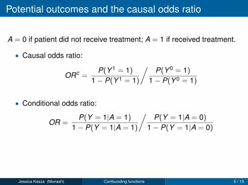
A = 0 if patient did not receive treatment; A = 1 if received treatment.
• Causal odds ratio:
ORc =P(Y 1 = 1)
1− P(Y 1 = 1)
/P(Y 0 = 1)
1− P(Y 0 = 1)
• Conditional odds ratio:
OR =P(Y = 1|A = 1)
1− P(Y = 1|A = 1)
/P(Y = 1|A = 0)
1− P(Y = 1|A = 0)
If causal inference assumptions are satisfied, ORc = OR.
Jessica Kasza (Monash) Confounding functions 5 / 15
Potential outcomes and the causal odds ratio
A = 0 if patient did not receive treatment; A = 1 if received treatment.
• Causal odds ratio:
ORc =P(Y 1 = 1)
1− P(Y 1 = 1)
/P(Y 0 = 1)
1− P(Y 0 = 1)
• Conditional odds ratio:
OR =P(Y = 1|A = 1)
1− P(Y = 1|A = 1)
/P(Y = 1|A = 0)
1− P(Y = 1|A = 0)
If causal inference assumptions are satisfied, ORc = OR.
Jessica Kasza (Monash) Confounding functions 5 / 15

Differences between treatment groups
• If data are observational, likely to be differences betweentreatment groups.
• Measured confounders:• e.g. treated subjects tend to be older & older patients more likely to
experience the outcome.• Unmeasured confounders:
• e.g. cognitive function; social connectedness; some measure ofoverall health.
• Adjusting for measured confounders:• Assume an inverse probability of treatment weighting approach
used to estimate a marginal odds ratio.• Skip the details!
How can we adjust for the unmeasured differences that wesuspect are present?
Jessica Kasza (Monash) Confounding functions 6 / 15
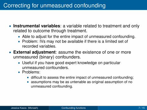
Correcting for unmeasured confounding
• Instrumental variables: a variable related to treatment and onlyrelated to outcome through treatment.
• Able to adjust for the entire impact of unmeasured confounding.• Problem: IVs may not be available if there is a limited set of
recorded variables.• External adjustment: assume the existence of one or more
unmeasured (binary) confounders.• Useful if you have good expert knowledge on particular
unmeasured confounders.• Problems:
• difficult to assess the entire impact of unmeasured confounding;• assumptions may be as untenable as original assumption of no
unmeasured confounding.
Jessica Kasza (Monash) Confounding functions 7 / 15

Confounding function approach1
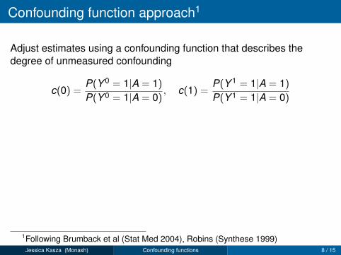
Adjust estimates using a confounding function that describes thedegree of unmeasured confounding
c(a) =P(Y a = 1|A = 1)P(Y a = 1|A = 0)
, a = 0,1
• c(0), c(1) are a counterfactual quantities: values selected byinvestigators.
• Requires contextual knowledge to quantify the impact ofunmeasured confounding, in terms of counterfactual outcomes.
What differences in the outcomes are due to unaccounted-fordifferences in the treatment groups, rather than due to the effect oftreatment on the outcome?
1Following Brumback et al (Stat Med 2004), Robins (Synthese 1999)Jessica Kasza (Monash) Confounding functions 8 / 15
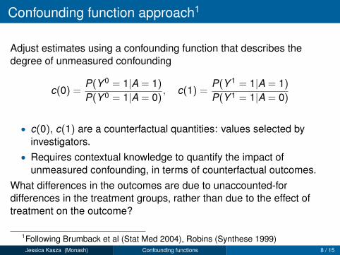
Confounding function approach1
Adjust estimates using a confounding function that describes thedegree of unmeasured confounding
c(0) =P(Y 0 = 1|A = 1)P(Y 0 = 1|A = 0)
, c(1) =P(Y 1 = 1|A = 1)P(Y 1 = 1|A = 0)
• c(0), c(1) are a counterfactual quantities: values selected byinvestigators.
• Requires contextual knowledge to quantify the impact ofunmeasured confounding, in terms of counterfactual outcomes.
What differences in the outcomes are due to unaccounted-fordifferences in the treatment groups, rather than due to the effect oftreatment on the outcome?
1Following Brumback et al (Stat Med 2004), Robins (Synthese 1999)Jessica Kasza (Monash) Confounding functions 8 / 15

Confounding function approach
A = 0⇒ no treatment, A = 1⇒ received treatment:
c(0) =P(Y 0 = 1|A = 1)P(Y 0 = 1|A = 0)
, c(1) =P(Y 1 = 1|A = 1)P(Y 1 = 1|A = 0)
c(0) = c(1) = 1⇒• No unmeasured confounding is present.
c(0) > 1, c(1) > 1, c(0) = c(1)⇒• Risk of (both) potential outcomes higher among those actually
treated.• Some of the observed risk of the outcome for treated subjects is
due to some unmeasured ‘ill health’;• Effect of treatment the same in treated and untreated groups.
Jessica Kasza (Monash) Confounding functions 9 / 15

Adjusting for unmeasured confounding
ORc =P(Y 1 = 1)
1− P(Y 1 = 1)
/P(Y 0 = 1)
1− P(Y 0 = 1)
c(a) =P(Y a = 1|A = 1)P(Y a = 1|A = 0)
, h(a) = P(A = 0) + c(a)P(A = 1)
The causal odds ratio can be written as:
ORc =h(1)P(Y = 1|A = 1)/c(1)
1− h(1)P(Y = 1|A = 1)/c(1)
/h(0)P(Y = 1|A = 0)
1− h(0)P(Y = 1|A = 0)
• Consider sensitivity of OR to range of values of c(1) and c(0).• Beware implicit assumptions if c(1) 6= c(0): differential treatment
effect in treated and untreated.
Jessica Kasza (Monash) Confounding functions 10 / 15

Application: Abciximab and death2
996 percutaneouscoronary inter-vention patients
Abciximab:698 (70%)
No abciximab:298 (30%)
11 died(1.6% of 698)
15 died(5.0% of 298)
• Administration of abciximab at discretion of interventionist.• Adjust for sex, height, diabetes, recent MI, left ventricle ejection
fraction, number of vessels in PCI, insertion of coronary stentusing inverse probability of treatment weighting.
OR = 0.17,95% CI (0.08,0.46)
2Data from twang R package, originally analysed in Kereiakes et al, AmHeart J (2000)
Jessica Kasza (Monash) Confounding functions 11 / 15
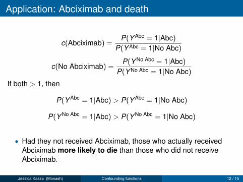
Application: Abciximab and death
c(Abciximab) =P(Y Abc = 1|Abc)
P(Y Abc = 1|No Abc)
c(No Abciximab) =P(Y No Abc = 1|Abc)
P(Y No Abc = 1|No Abc)
If both > 1, then
P(Y Abc = 1|Abc) > P(Y Abc = 1|No Abc)
P(Y No Abc = 1|Abc) > P(Y No Abc = 1|No Abc)
• Had they not received Abciximab, those who actually receivedAbciximab more likely to die than those who did not receiveAbciximab.
Jessica Kasza (Monash) Confounding functions 12 / 15

Sensitivity analysis for the OR
.8.9
11.
11.
21.
3c(
0)
.8 .9 1 1.1 1.2 1.3c(1)
c(0) = 1 c(1) = 1 c(0) = c(1)
0.13
0.14
0.15
0.16
0.17
0.18
0.19
0.20
0.21
0.22
Odd
s ra
tio
Jessica Kasza (Monash) Confounding functions 13 / 15

Sensitivity analysis for the OR, c(0) = c(1) = 1
.2.4
.6O
R
.8 .9 1 1.1 1.2 1.3Confounding function value
Jessica Kasza (Monash) Confounding functions 14 / 15

Take-home messages
• Causal inference is useful in situations when randomised trialscan’t be conducted
• Strict assumptions, including no unmeasured confounding.• Problem: in most applications, the assumption of unmeasured
confounders will not be satisfied!• Turn to alternative approaches:
• Instrumental variables; external adjustment; confounding functions.• I’ve described the confounding function approach for binary
outcomes.• Approach also available for continuous outcomes.• Provides a way to assess the sensitivity of estimates to the entire
effect of unmeasured confounding.• Easy to apply.• Contact me for Stata code!
Jessica Kasza (Monash) Confounding functions 15 / 15

References
• VanderWeele TJ, Arah OA. (2011) Bias formulas for sensitivityanalysis of unmeasured confounding for general outcomes,treatments, and confounders. Epidemiology, 22:42-52.
• Robins JM. (1999) Association, causation and marginal structuralmodels. Synthese, 121:151-79.
• Brumback BA, Hernan MA, Haneuse SJPA, et al. (2004)Sensitivity analyses for unmeasured confounding assuming amarginal structural model for repeated measures. Statistics inMedicine, 23:749-767.
Jessica Kasza (Monash) Confounding functions 16 / 15

Propensity scores
• Propensity score for subject i , with observed covariates Xi = xi ,treatment Ai = ai :
PSi = P(Ai = 1|Xi = xi)
Usually estimated using logistic regression models.• Rosenbaum & Rubin (Biometrika, 1983): adjustment for PS
sufficient to remove bias due to all X .• Inverse probability of treatment weighting: Each subject’s
observation assigned a weight:
wi =ai
PSi+
1− ai
1− PSi
• Each subject’s observation weighted by 1/wi .
Jessica Kasza (Monash) Confounding functions 17 / 15