Advances in Water Resources 32 (2009) 147–158

Contents lists available at ScienceDirect

Advances in Water Resources

journal homepage: www.elsevier .com/ locate/advwatres

Assessing the impact of land use change on hydrology by ensemble modelling(LUCHEM) II: Ensemble combinations and predictions

Neil R. Viney a,*, H. Bormann b, L. Breuer c, A. Bronstert d, B.F.W. Croke e, H. Frede c, T. Gräff d, L. Hubrechts f,J.A. Huisman g, A.J. Jakeman e, G.W. Kite h, J. Lanini i, G. Leavesley j, D.P. Lettenmaier i, G. Lindström k,J. Seibert l, M. Sivapalan m,1, P. Willems n

a CSIRO Land and Water, GPO Box 1666, Canberra, ACT 2600, Australiab Institute for Biology and Environmental Sciences, Carl von Ossietzsky University, Oldenburg, Germanyc Institute for Landscape Ecology and Resources Management, Justus-Liebig University, Giessen, Germanyd Institute for Geoecology, University of Potsdam, Germanye Integrated Catchment Assessment and Management Centre, The Australian National University, Canberra, Australiaf Afdeling Ecologie en Water, Lisec NV, Genk, Belgiumg ICG-4 Agrosphere, Forschungszentrum Jülich, Germanyh Hydrologic Solutions, Pantymwyn, United Kingdomi Department of Civil and Environmental Engineering, University of Washington, Seattle, WA, USAj United States Geological Survey, Denver, CO, USAk Swedish Meteorological and Hydrological Institute, Norrköping, Swedenl Department of Physical Geography and Quaternary Geology, Stockholm University, Stockholm, Swedenm Centre for Water Research, University of Western Australia, Perth, Australian Hydraulics Laboratory, Katholieke Universiteit Leuven, Belgium

a r t i c l e i n f o

Article history:Received 13 July 2007Received in revised form 20 May 2008Accepted 22 May 2008Available online 5 June 2008

Keywords:Multi-model ensemblesSingle-model ensemblesCatchment modellingEnsemble combinationUncertaintyLand use change

0309-1708/$ - see front matter Crown Copyright � 2doi:10.1016/j.advwatres.2008.05.006

* Corresponding author.E-mail address: neil.viney@csiro.au (N.R. Viney).

1 Present address: Department of Geography, UnChampaign, IL, USA.

a b s t r a c t

This paper reports on a project to compare predictions from a range of catchment models applied to amesoscale river basin in central Germany and to assess various ensemble predictions of catchmentstreamflow. The models encompass a large range in inherent complexity and input requirements. Inapproximate order of decreasing complexity, they are DHSVM, MIKE-SHE, TOPLATS, WASIM-ETH, SWAT,PRMS, SLURP, HBV, LASCAM and IHACRES. The models are calibrated twice using different sets of inputdata. The two predictions from each model are then combined by simple averaging to produce a single-model ensemble. The 10 resulting single-model ensembles are combined in various ways to producemulti-model ensemble predictions. Both the single-model ensembles and the multi-model ensemblesare shown to give predictions that are generally superior to those of their respective constituent models,both during a 7-year calibration period and a 9-year validation period. This occurs despite a considerabledisparity in performance of the individual models. Even the weakest of models is shown to contributeuseful information to the ensembles they are part of. The best model combination methods are a trimmedmean (constructed using the central four or six predictions each day) and a weighted mean ensemble(with weights calculated from calibration performance) that places relatively large weights on the betterperforming models. Conditional ensembles, in which separate model weights are used in different systemstates (e.g. summer and winter, high and low flows) generally yield little improvement over the weightedmean ensemble. However a conditional ensemble that discriminates between rising and receding flowsshows moderate improvement. An analysis of ensemble predictions shows that the best ensembles arenot necessarily those containing the best individual models. Conversely, it appears that some models thatpredict well individually do not necessarily combine well with other models in multi-model ensembles.The reasons behind these observations may relate to the effects of the weighting schemes, non-stationa-rity of the climate series and possible cross-correlations between models.

Crown Copyright � 2008 Published by Elsevier Ltd. All rights reserved.

008 Published by Elsevier Ltd. All r

iversity of Illinois, Urbana-

1. Introduction

A model is a simplified conceptualization of a complex, possiblychaotic system, which is often characterized by highly variablebehaviour in space and time. As such, no model, particularly those

ights reserved.

148 N.R. Viney et al. / Advances in Water Resources 32 (2009) 147–158

associated with natural systems, can ever provide a perfect realiza-tion. Indeed, it can even sometimes be difficult to quantify the de-gree of uncertainty in input data, model structure and modelparameterization. Taken together, these uncertainties inevitablylead to considerable uncertainty in model predictions. One of theways of addressing some of these uncertainty issues is throughensemble modelling. The term ‘ensemble modelling’ encompassesa large range of approaches to producing predictions of fluxes andproperties. A single-model ensemble involves the use of a numberof realizations of a single deterministic model. Distinct predictionsare obtained for each realization by either perturbing the inputdata or initial conditions, or by selecting different sets of modelparameters. These perturbations may be stochastic or determinis-tic (e.g. derived from alternative sources). In a multi-model ensem-ble, several different deterministic models are used. Theserealizations may or may not use a common input data set.

Ensemble modelling has often been used in the climate andatmospheric sciences, where operational ensembles have been inuse for well over a decade. Most studies of the accuracy of multi-model ensemble forecasts in weather prediction report that theytend to outperform individual models [9] and that multi-modelensembles tend to perform better than single-model ensembles[28]. Ensemble modelling has the potential to assist in providingbetter understanding of the physical processes and in informingthe development of better models [7,23].

Until relatively recently, however, ensemble modelling has re-ceived little attention in hydrology, where most modelling studiesuse only one model. There have been several studies comparingpredictions from various hydrological models (e.g., [27,19]). In gen-eral, these studies have been limited to describing how differentmodels and different modelling approaches can affect predictionaccuracy, but usually have not considered the issue of poolingmodel predictions to arrive at some consensus prediction.

Recently, some new cooperative initiatives such as the Distrib-uted Model Intercomparison Project (DMIP) and the EnsembleStreamflow Prediction (ESP) project in the United States and theinternational Hydrological Ensemble Prediction Experiment (HEP-EX) have begun to explore ensemble modelling in a hydrologicalsetting. These projects are aimed primarily at using single-modelensembles to produce short term streamflow forecasts conditionedon climate forecasts (e.g., [6,11,13]). Other ensemble research hasfocussed on combining predictions using different parameter setsfrom a single model structure (e.g., [16]).

The first published study on multi-member hydrologic ensem-bles appears to be that of Shamseldin et al. [23], in which ensemblepredictions are constructed using five rainfall-runoff models ap-plied to 11 catchments. They assessed combinations involving sim-ple averaging, a regression-based scheme and a neural networkscheme. While the results are inconsistent from one catchmentto another, Shamseldin et al. conclude that the combined modelsgenerally produce better predictions than the single models.Georgakakos et al. [10], as part of DMIP, assessed predictions fromseven distributed models applied to six catchments in the UnitedStates. They found that a simple mean of the five best models ineach catchment consistently outperforms the best individual mod-el, but that a weighted mean ensemble, while usually better thanthe best model, is inferior to the simple mean ensemble. In a fur-ther analysis of the DMIP dataset, Ajami et al. [1] assessed the pre-dictions of several types of regression-based ensemble andconcluded that they are superior to predictions from an unbiasedaverage ensemble and from individual models. They also foundthat combination methods involving bias removal are desirable,but only in catchments with stationary flow conditions betweenthe calibration and validation periods.

To date, none of these projects have considered ensemble mod-elling of the hydrological impacts of land use change. This paper is

the second in a series of four describing the Land Use Change onHydrology by Ensemble Modelling (LUCHEM) project, which in-volves the application of 10 catchment models to a basin withnested gauges. The first paper [5] describes the background tothe project and analyses the individual performances of the 10models in predicting streamflows for current land use conditions.The third paper [12] describes the results of an application of these10 models to the prediction of the impacts of land use change andassesses the uncertainty in the land use change predictions. Thefourth paper [4] assesses the impact of changes in the resolutionof spatial input data on the streamflow predictions of three ofthe LUCHEM models.

In this paper, we assess the use and effectiveness of a number ofmodel ensembles made up of some or all of the individual models.In comparison with previous studies, this paper includes a largernumber of models with a large range of inherent model complexityand assesses a larger range of ensemble combination techniques.The following sections describe the modelling procedure and ana-lyse prediction accuracy both for the individual models and forseveral types of ensembles including all models.

2. The Dill River catchment

The Dill River in Hesse, Germany, is a tributary of the Lahn Riv-er, which ultimately flows westward into the Rhine River. The DillRiver at Asslar has a catchment area of 693 km2. The topography ofthe catchment is characterized by low mountains and has an alti-tude range of 155–674 m. The mean annual precipitation of the Dillcatchment varies from 700 mm in the south to more than1100 mm in the higher elevation areas in the north and also exhib-its a general west-east gradient. Areas with lower annual precipi-tation tend to have summer-dominated rainfall patterns, whilethe wetter parts of the catchment are dominated by winter precip-itation patterns. A small proportion (less than 5%) of winter precip-itation falls as snow, particularly at higher elevations. Refer toBreuer et al. [5] for further details on the catchment’s climate,topography, soil and land cover.

Streamflow in the Dill catchment is generated primarily frominterflow processes with relatively little baseflow and surface run-off. Mean annual streamflow for the period 1983–1998 is 438 mm(about 48% of catchment-averaged precipitation). There is a dis-tinct winter peak, with 77% of streamflow occurring in the sixmonths from November to April. There are, however, some signif-icant temporal trends in streamflow patterns during the 19-yearperiod used in this study. The mean annual streamflow recordedin the 1990s is about 20% less than that for the 1980s and thishas been accompanied by a significant reduction in runoff coeffi-cient. Most of the reduction in streamflow has occurred duringthe winter months. There is also some evidence that the winterpeak and the period of summer low flows are arriving about onemonth later during the 1990s than during the 1980s.

3. The models

Ten models with the capability of predicting the impacts of landuse change are applied to the Dill catchment. In approximatelydecreasing order of complexity, they are: DHSVM [26], MIKE-SHE[22], TOPLATS [20], WASIM-ETH [18], SWAT [2], PRMS [15], SLURP[14], HBV [3], LASCAM [24] and IHACRES [8]. In terms of their spa-tial resolution and the overall number of model parameters, themodels represent a broad cross-section of complexity ranging fromfully distributed, physically based models with explicit groundwa-ter schemes (DHSVM, MIKE-SHE) to fully lumped, conceptual mod-els (e.g. IHACRES). There are also other more subtle differencesamong the models, including differences in rainfall interpolation,

N.R. Viney et al. / Advances in Water Resources 32 (2009) 147–158 149

channel routing and estimation of potential evaporation. Somemodels use explicit snow accumulation routines, while others treatall precipitation as rainfall.

Each model was prepared, calibrated and operated either by itscreator or by a modeller with considerable familiarity in its use.Each modeller was provided with common digital maps of eleva-tion, soil type (discriminated into 149 soil classes and includingsoil physical characteristics) and land cover. Daily precipitation(16 sites) and weather (2 sites) data were provided, but modellerswere free to interpolate and re-process this data by any suitablemethod. Similarly, the calibration methods and objective functionswere different from model to model. All models were calibratedusing observed streamflow data for the period 1983–1989 andmodel predictions were developed for the validation period1990–1998. A maximum of 3 years of additional weather data(1980–1982) was available for model spin-up. All the models wereset up to provide spatially explicit predictions of streamflow at avariety of spatial scales across the catchment. Observed stream-flows from three gauged subcatchments were available to assessspatial predictions, but this paper is limited to the analysis of mod-el performance against the observed streamflows at Asslar. A moredetailed description of model characteristics, set-up proceduresand calibration procedures appears in Ref. [5].

The use of different data interpolation schemes by differentmodels resulted in a considerable range of predictions of basiccatchment water balance components like mean annual rainfall,actual evaporation and storage [5]. In an effort to minimise thesedifferences, a second calibration was performed for each model.In the second calibration procedure, modellers were restricted tousing common, pre-processed, high-resolution (25 m) fields of veg-etation density and daily precipitation (interpolated from the 16observation sites) and to using other climate data from a single,central observation station. They were invited to recalibrate theirmodels to a similar level of rigour as before and submit a secondset of model predictions for both the calibration and validationperiods. We refer to this as the homogeneous dataset, while thepredictions from the first calibration process are referred to asthe original dataset. For the MIKE-SHE model, predictions are avail-able only for the homogeneous dataset. More details on the cali-bration procedures and an analysis of prediction differencesbetween the two calibration processes are available in Ref. [5].

4. Ensemble construction

Although the second calibration was performed primarily tofacilitate better comparison of individual model performances, italso provides an opportunity for ensemble analysis. For each model(except MIKE-SHE), we have two semi-independent realizations offlow predictions, one for the original calibration and one for the cal-ibration using the homogeneous dataset. We may combine theseinto a single time series of flow predictions for each model by takingthe mean of the two predictions. This resulting time series will be re-ferred to as a single-model ensemble (SME). We now use these SMEs(along with the homogeneous predictions of MIKE-SHE) as membersof several different types of multi-model ensemble (MME).

Ensemble predictions may be constructed in a number of ways.Perhaps the simplest is the approach we used to construct theSMEs, which is to take the raw mean of the model predictionsfor each day. Another simple ensemble prediction is to adopt thedaily median of all ensemble members. In this study, where 10models are available, the median is given by the mean of the fifthand sixth highest predictions. Ensembles may also be constructedby including a subset of the 10 models (e.g. the mean of the bestthree models in calibration). A further elaboration might be to in-clude a mixture of two or more subset ensembles, with the switch-

ing between ensembles conditioned upon some attribute of theflow regime or climate. In this paper, we assess the performancesof the following ensembles:

� mean of all models,� median of all models,� trimmed mean (excluding extreme predictions),� multiple linear regression of all models,� principal components regression,� Bayesian model averaging,� means of all permutations of models ranging from 1 to 10

members,� weighted mean of all models (weighted by calibration

performance),� weighted means of all permutations of models,� conditional ensembles based on season,� conditional ensembles based on flow stage (i.e. rising or falling),� conditional ensembles based on flow level (i.e. high and low

flows).

In the cases of the regression ensembles, the weighted ensem-bles and the conditional ensembles, the ensemble members andtheir relative weightings are determined using predictions fromthe calibration period only. These weighting are then applied with-out adjustment during the validation period. For example, for themulti-variable linear regression ensemble, regression coefficientsare established during the calibration period and applied un-changed during the validation period.

The multiple linear regression ensemble is constructed by usingthe 10 SMEs as the independent variables and the observed flow inthe calibration period as the dependent variable. Given the highcorrelation between efficiency and the square of the correlationcoefficient for values of both approaching one, it is reasonable toexpect that the unconstrained multiple linear regression ensemblerepresents the optimal linear combination of model predictionsduring the calibration phase and it should therefore give betterefficiencies than the raw mean, the trimmed means and theweighted means – all of which are inferior linear combinations –and any individual model. The regression ensemble must also havezero bias during the calibration period. However, none of theseproperties will necessarily hold for the validation period. One dis-advantage of the regression approaches is that they might includea non-zero intercept. This could result in a nonzero ensemble flowprediction even when all models are predicting zero flow. Regres-sion ensembles might also involve negative coefficients for somemodels and this too can potentially result in negative flow predic-tions. To partially overcome these issues we also assess two con-strained (zero-intercept) multiple regressions: one involving all10 models and one including only those models with positiveand significantly non-zero coefficients.

Where there is multicollinearity between the independent vari-ables (the individual SMEs) the predictions of a multiple linearregression model may have reduced reliability. Principal compo-nents regression (PCR) has been proposed as a method for copingwith this collinearity by transforming the predictor variables intoa set of orthogonal variables called principal components. Theseorthogonal variables (or a subset of them) are then suitable foruse in ordinary least squares regression. In this study we assessthe predictions of PCR ensembles constructed from 1, 2, 3 and 4principal components.

Recently, a Bayesian model averaging (BMA) method was pro-posed to optimally combine the predictions of a multi-modelensemble [21,25]. The BMA predictive model can be expressed as

pðDkf1; . . . ; fnÞ ¼Xn

i¼1

wigiðDkfiÞ;

150 N.R. Viney et al. / Advances in Water Resources 32 (2009) 147–158

where f is the predictions for each ensemble member, wi is theweight of the ith model and gi(Dkfi) can be interpreted as theprobability density function (PDF) of the measurement giventhe forecast, conditional on the prediction being the best predictionin the ensemble. The weights can be interpreted as the individualmodel’s relative contribution to predictive skill of the ensemble.They are positive and add up to one. In the original approach of Raf-tery et al. [21], the conditional PDF gi(Dkfi) can be approximatedwith a normal distribution centred on a bias-corrected forecastand having a variance r2 as

Dkfi � Nðai þ bifi;r2Þ;

where ai and bi are bias correction terms that are derived from linearregression between measurement and prediction for the training(calibration) period. Vrugt et al. [25] showed that the use of the intu-itively more appropriate gamma distribution did not improve theperformance of the BMA method. They did, however, argue thatthe linear bias correction is too simplistic for streamflow data, andsuggested instead to consider a heteroscedastic error with r2 = b � fi,where b is a slope parameter that relates the forecast to the variance.

The BMA approach requires the specification of the modelweights, the variance and the slope parameter when a heterosced-astic error is assumed. Following Vrugt et al. [25], we estimatethese parameters by posing an optimization problem in a maxi-mum likelihood context. A global optimization algorithm is usedto maximize the log-likelihood function

lðhÞ ¼X

t

logXn

i¼1

wigiðDtkfitÞ;

where h denotes the parameters to be estimated and the summingis over all observation times t in the training period. After optimiza-tion, the deterministic BMA ensemble prediction is simply given by

EðDkf1; . . . fnÞ ¼Xn

i¼1

wifi:

In this study, we consider four BMA analyses. The first two consistof the original approach of Raftery et al. [21] with and without biascorrection and the other two consider a heteroscedastic error withand without bias correction.

Other ensembles may be constructed by weighting the relativecontributions of the models or by using subsets of the 10 models.For example, one of the trimmed mean ensembles is calculatedby eliminating the highest and lowest model prediction each dayand calculating a mean ensemble prediction from the predictedflows of the remaining eight models. Similar trimmed ensemblesmay be constructed from the six or four centremost predictionseach day. We would expect the predictions of the three trimmedensembles to lie between those of the mean and median, withthe eight-model trimmed mean being nearest to the meanand the four-member trimmed mean being nearest to the median.The mean and median ensembles are equivalent to a 10-modeltrimmed mean and a two-model trimmed mean, respectively.

In the weighted ensembles, the weightings for each model mustbe calculated from some statistical property of the model’s calibra-tion predictions. A suitable statistic to use is the inverse of themean square error. This is equivalent to weighting by 1/(1 � E),where E is the model’s calibration efficiency [17]. If we also intro-duce an optional exponent, k, then the weighting for the ith modelis given by

Wiðn; kÞ ¼1

ð1� EiÞkXn

i¼1

1

ð1� EiÞk

!,;

where n is the number of models in the ensemble. In this way (pro-vided k is positive), the models with the largest calibration efficien-cies make the largest contributions to the weighted ensemble in both

calibration and validation periods. The case where k = 1 is equivalentto weighting by 1/(1 � E), while the case where k = 0 represents theunweighted mean. The limit as k tends to infinity is equivalent tousing the best SME. Thus, the rationale for allowing different valuesof k is that they allow us to examine ensembles with differeing de-grees of relative dominance of the better performing models.

With each unweighted or weighted mean having up to 10 po-tential members, there is a total of 1023 permutations of MME,ranging from the 10 one-model MMEs (i.e. the 10 SMEs) to the sin-gle 10-model MME. For example, there are 252 possible combina-tions of five-member MMEs. In this paper, we assess all possiblepermutations.

It is recognized that some models may perform better on someparts of the hydrograph than on others. For example, a model mayprovide better predictions of summer flows than of winter flows.This is clearly a possibility given that some of the models includesnow accumulation and melting routines while others do not. Thisraises the possibility that better overall predictions might be ob-tained by using different combinations of models (weighted ornot) for different parts of the hydrograph. This approach we referto as conditional ensembling. Three conditional ensembles are as-sessed here. As well as assessing the use of separate summer (de-fined here as May–October) and winter (November–April) MMEs,we also consider separate MMEs for rising and falling flows, andfor high and low flows.

For each conditional ensemble it is a requirement that the sep-arate MMEs be constructed using data from the calibration periodonly. For application to the validation period, we, therefore, need away of discriminating between the two cases. Furthermore, thisdiscrimination must be based on the SME predictions only, notthe observed hydrographs. After some preliminary analysis, it hasbeen found that defining days with rising flows as days on whichat least five of the SME predictions are rising is the best indicatorof rising flows in the observed record. Days with fewer than fiverising SMEs are classified as receding. This includes days with staticor zero flows. This scheme has a prediction success rate of 83% dur-ing the calibration period. According to this classification criterion,rising flows occur on 28% of days and carry 41% of the total flow.The demarcation for high and low flows is taken as days with themean MME prediction above and below 1 mm. Mean MME predic-tions in excess of 1 mm occur on 37% of days and account for 78%of the total flow. Of course, given that most of the flow, and there-fore most of the large flow events, occur in winter, it is possiblethat the flow-dependent conditional ensemble will yield similarresults to the seasonal ensemble.

With the emphasis in the LUCHEM project being on predictingthe impacts of land use change, we do not consider assessing someof the sequential data assimilation techniques (e.g. the ensembleKalman filter) that have recently been applied with some successto operational or experimental forecasting ensembles (e.g., [13,25]).

There are many potential metrics of prediction quality. In thisstudy, we restrict ourselves to assessing model performance usingthe Nash–Sutcliffe efficiency calculated on daily flows, and the to-tal bias. The former gives a measure of how well a model repro-duces the fine-scale aspects of the observed time series (albeitbiased towards high flows), while the latter assesses the long-termprediction quality.

5. Model predictions

5.1. Predictions of individual models

Breuer et al. [5] report on the calibration and validation perfor-mances of the individual models. A brief recap of their results is gi-ven here.

0.6 0.65 0.7 0.75 0.8 0.85 0.9−5

0

5

10

15

20

25

SWAT

DHSVM

MIKESHE

HBVTOPLATS

SLURP

IHACRES

LASCAM

PRMS

WASIMETH

Efficiency

Bias

(pe

rcen

t)

ValidationCalibration

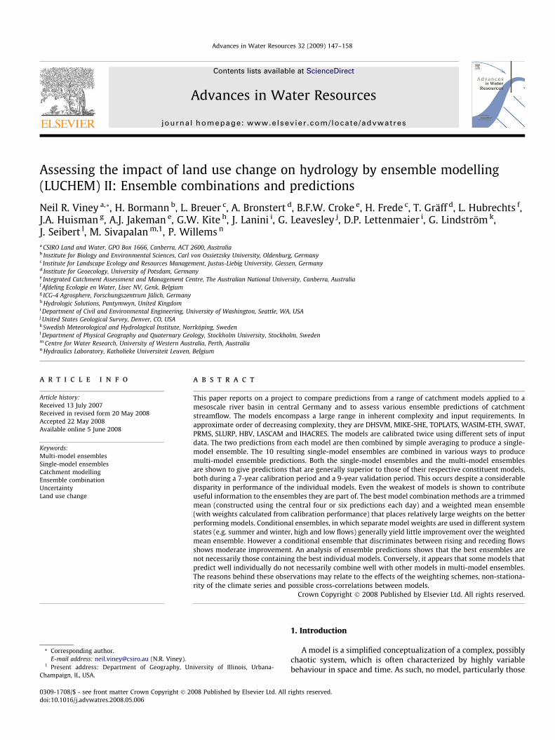
Fig. 3. As for Fig. 2, but for the homogeneous dataset.

N.R. Viney et al. / Advances in Water Resources 32 (2009) 147–158 151

A time series of model predictions is shown in Fig. 1 for part ofthe calibration period. Qualitatively, the models are shown to beproviding good predictions of the observed streamflow in termsof timing and magnitude of events. The envelope defined by therange of model predictions encompasses the observed streamflowon 96% of days, with little difference between calibration and val-idation periods. When this envelope is trimmed to eliminate thelargest and smallest prediction, it still includes the observedstreamflow on 83% of days. On average, the daily minimum predic-tion is 52% of the observed flow and the daily maximum predictionis 171% of the observed flow.

Scatter plots for two of the performance statistics (daily Nash–Sutcliffe efficiency and bias) for each of the models are shown inFig. 2 for the original case. Statistically, the best models are thosewith efficiencies approaching 1.0 and biases near 0%. For the cali-bration period (open circles), all but two of the models have nega-tive biases (i.e. they underpredict). However, no model has anabsolute bias as high as 10%. The calibration efficiencies range fromabout 0.6 to 0.9, with the less complex models tending to havehigher values.

January February March April May June0

2

4

6

8

10

12

Stre

amflo

w (

mm

)

Fig. 1. Time series of observed streamflow (thick black line) in the Dill catchment,1983, together with the various model predictions for the homogeneous dataset(thin coloured lines). The names of the individual models are immaterial.

0.55 0.6 0.65 0.7 0.75 0.8 0.85 0.9 0.95−15

−10

−5

0

5

10

15

SWAT

DHSVM

HBVTOPLATS

SLURP

IHACRES

LASCAM

PRMS

WASIMETH

Efficiency

Bias

(pe

rcen

t)

ValidationCalibration

Fig. 2. Bias and efficiency of model predictions for the original dataset for thecalibration (open circles) and validation (solid circles) periods. There are nopredictions of the MIKE-SHE model available for the original dataset.

When the predictions in the validation period are assessed (so-lid circles in Fig. 2), the relative positions of the models remain lar-gely unchanged. However, nine of the 10 models have increased(i.e. more positive) biases, to the extent that they are all now over-predicting. All but one of the models also have increased efficien-cies in the validation period.

For some models the differences in calibration statistics be-tween the original and homogeneous datasets are quite small, withthe latter typically yielding slightly better efficiencies and slightlymore positive bias. However, for other models, especially DHSVMand WASIM-ETH, efficiencies decline and bias increases substan-tially. When the homogenized calibrations are used in the valida-tion period (Fig. 3), once again, most models have increasedbiases and, except for LASCAM and TOPLATS, also have increasedefficiencies. The trajectories of movement between calibrationand validation are similar to those in Fig. 2.

5.2. Single-model ensembles

The bias and efficiency of the SMEs are compared to those of theindividual calibrations in Fig. 4 and Table 1. By definition, the biasof a SME constructed from the mean of its members is equal to the

0.55 0.6 0.65 0.7 0.75 0.8 0.85 0.9 0.95−15

−10

−5

0

5

10

15

20

25

SWAT

DHSVM

MIKE−SHE

HBV

TOPLATS

SLURP

IHACRES

LASCAM

PRMS

WASIM−ETH

Original

Homogeneous

SME

Efficiency

Bia

s (

%)

Fig. 4. Bias and efficiency of single-model ensembles for the validation period,compared with the corresponding statistics for the original and homogeneousdatasets.

Table 1Calibration and validation efficiencies for the original and homogeneous data sets andthe SMEs

Model Calibration Validation

Orig. Homog. SME Orig. Homog. SME

DHSVM 0.803 0.760 0.803 0.873 0.849 0.878MIKE-SHE – 0.647 0.647 – 0.732 0.732TOPLATS 0.593 0.656 0.670 0.551 0.611 0.648WASIM 0.740 0.703 0.742 0.750 0.743 0.768SWAT 0.721 0.730 0.726 0.729 0.738 0.733PRMS 0.845 0.845 0.845 0.880 0.880 0.880SLURP 0.625 0.655 0.644 0.715 0.708 0.715HBV 0.907 0.918 0.913 0.914 0.925 0.921LASCAM 0.895 0.897 0.897 0.898 0.890 0.895IHACRES 0.818 0.817 0.818 0.867 0.865 0.866

0.89 0.9 0.91 0.92 0.93 0.94 0.95−3

−2

−1

0

1

2

3

4

5

6

7

A1

B1

B2

B3B4B5

C1

C2

C3

D1 D2 D3 D4E1

E2

E3

E4

F2F3 F4

G1 G2

G3

H1H2

H3H4

I1

I2I3

CalibrationValidation

Efficiency

Bias

(%

)

Fig. 5. Bias and efficiency of selected multi-model ensembles for the calibration(open circles) and validation (closed circles) periods, compared with the corre-sponding statistics for the best single-model ensemble. Labels for each ensembleare defined in Table 2.

Table 2Bias and efficiency of selected MMEs for the calibration and validation periods

MME Calibration Validation

Bias (%) Efficiency Bias (%) Efficiency

A1. Best SME �0.6 0.913 4.9 0.921B1. Mean 0.2 0.910 5.5 0.930B2. Trimmed Mean (8 models) �1.8 0.905 3.8 0.936B3. Trimmed Mean (6 models) �2.4 0.903 3.2 0.937B4. Trimmed Mean (4 models) �2.7 0.897 2.7 0.938B5. Median �2.8 0.893 2.4 0.936C1. Linear regression (unconstrained) 0.0 0.948 5.6 0.932C2. Linear regression (constrained) �1.5 0.948 3.5 0.932C3. Linear reg. (constrained, coeff>0) 1.7 0.944 7.2 0.932D1. PCR (1 component) 0.0 0.923 3.4 0.921D2. PCR (2 components) 0.0 0.929 4.0 0.923D3. PCR (3 components) 0.0 0.934 4.9 0.924D4. PCR (4 components) 0.0 0.938 4.6 0.923E1. BMA (homoscedastic) 0.1 0.922 5.0 0.928E2. BMA (homoscedastic, unbiased) �1.8 0.923 4.2 0.934E3. BMA (heteroscedastic) 0.2 0.921 5.1 0.931E4. BMA (heteroscedastic, unbiased) �1.6 0.927 4.0 0.933F2. Weighted 10-model (k = 0.5) �0.2 0.918 5.2 0.935F3. Weighted 10-model (k = 1.0) �0.5 0.925 4.9 0.937F4. Weighted 10-model (k = 1.5) �0.8 0.930 4.7 0.938G1. Seasonal 10-model (k = 1.5) �1.1 0.930 4.2 0.938G2. Rising/falling 10-model (k = 1.5) �1.3 0.934 4.0 0.941G3. High/low 10-model (k = 1.5) �0.4 0.930 4.2 0.939H1. Best unweighted calibration 0.5 0.936 5.6 0.928H2. Best weighted calib. (k = 0.5) 0.1 0.940 5.5 0.934H3. Best weighted calib. (k = 1.0) �0.4 0.942 5.4 0.936H4. Best weighted calib. (k = 1.5) �0.8 0.942 5.2 0.935I1. Best seasonal (k = 1.5) �1.3 0.943 3.8 0.936I2. Best rising/falling (k = 1.5) 0.1 0.946 5.5 0.933I3. Best high/low flow (k = 1.5) 0.1 0.942 4.8 0.936

152 N.R. Viney et al. / Advances in Water Resources 32 (2009) 147–158

mean of the biases of the two model realizations. However, in bothcalibration and validation periods, the efficiency of the SME is al-ways greater than the mean efficiency of the two ensemble mem-bers. In fact, in three of the nine calibration cases and four of thenine validation cases, the ensemble efficiency exceeds those ofboth ensemble members. These include both time periods forTOPLATS and WASIM-ETH.

5.3. Multi-model ensembles using simple averaging

In this section, we use the predictions of the SMEs calculatedabove (along with the homogeneous predictions of MIKE-SHE) asmembers of several different types of simple multi-model ensem-bles that are based on raw averages.

The prediction capabilities of selected simple MMEs (labelledwith the letter B) are shown in Fig. 5 and Table 2. The mean ensem-ble has the best efficiency in the calibration period and the medianhas the worst. However, in the validation periods, the median hasthe largest increase in efficiency of the simple ensembles and thesmallest increase in bias. All five ensembles improve in efficiencyin the validation period. The mean always has a larger (i.e. morepositive) bias than the median for both calibration and validationperiods.

Interestingly, although the raw mean is a simple ensemble andincludes contributions from some models that have quite modestperformance statistics, its validation efficiency is still superior to

that of the best SME. Similarly, the trimmed mean and medianensembles, despite having poorer calibration statistics than thebest SME are all clearly better than the best SME in the validationperiod.

5.4. Regression-based ensembles

The multiple linear regression ensemble (C1 in Fig. 5 and Table2) has the best calibration efficiency of any model tested in thisstudy, but unlike the simple averaging ensembles, its performancedegrades significantly between the calibration and validation peri-ods (in both bias and efficiency). Its validation efficiency is inferiorto those of the median and trimmed mean ensembles, and its val-idation bias is larger than any other ensemble in Fig. 5 and Table 2.

In the multiple linear regression ensemble, there is considerablemulticollinearity between the independent variables. Cross-corre-lation coefficients of up to 0.96 are observed between some pairsof SMEs. Furthermore, three of the SMEs have negative coefficientsin the linear regression ensemble, while two others have negativecoefficients that are not significantly different to zero. When theintercept is constrained to zero (C2 in Fig. 5 and Table 2) efficien-cies are identical to the unconstrained case, but biases are morenegative, for both calibration and validation. When we further lim-it the regression by eliminating SMEs with negative or non-signif-icant coefficients (C3 in Fig. 5 and Table 2) the efficiency invalidation is depressed slightly, but in validation it is unchanged.However, biases are significantly more positive than any otherensemble in Fig. 5 and Table 2.

Principal components regression can be used to overcome someof the problems with linear regression methods. PCR ensembles areconstructed for p = 1, . . . ,4, where p is the number of principalcomponents used. The resulting ensemble statistics are presentedin Fig. 5 and Table 2 (ensembles D1–D4). There is an increase incalibration efficiency as more components are added, but little

N.R. Viney et al. / Advances in Water Resources 32 (2009) 147–158 153

improvement in validation efficiencies. As was the case for the lin-ear regression MME, the PCR ensembles all have efficiencies thatdecline in the validation period. In both calibration and validation,the PCR efficiencies are less than those of the linear regressionMME.

5.5. Bayesian model averaging ensembles

Results of the BMA analyses are presented in Fig. 5 and Table 2(ensembles E1–E4). There is little difference between the perfor-mances of the two error models. However, the use of the linear biascorrection slightly improves efficiency in both error models andalso leads to lower (more negative) prediction biases. Unlike thelinear regression and PCR methods, the BMA ensembles yield effi-ciencies that are greater in the validation period than in the cali-bration period.

5.6. Unweighted and weighted selective ensembles

Fig. 6 shows the ranges of calibration and validation efficienciesfor the various permutations of unweighted mean MMEs and pro-vides further demonstration of the effectiveness of ensembling. Forboth calibration and validation, there is a clear trend towards in-creased median efficiencies and decreased ranges of efficiency asthe number of models in a MME increases. In both cases, the max-imum efficiency occurs for n = 5, but this occurs for different com-binations of models. All MMEs with three or more members(n P 3) have efficiencies greater than the median of the respectiveSMEs (n = 1). In calibration, 49% of ensembles with n > 1 have effi-ciencies that exceed the highest efficiency of their constituentSMEs, while in validation, this number increases to 75%. For all val-ues of n, the validation efficiencies exceed those of calibration.

Next, we investigate which combinations of models are likely toproduce the greatest increases in prediction efficiency. For each ofthe permutations with n > 1, we can calculate the variance of effi-ciencies of the constituent SMEs. We then divide the population ofMMEs into three groups: those with the lowest third of variances(i.e. those MMEs whose members have the most similar efficien-cies), those with the highest third of variances (i.e. those whosemembers have widely differing efficiencies) and those with themiddle third. In the calibration period, 85% of the ensembles withthe lowest variances have ensemble efficiencies that exceed the

1 2 3 4 5 6 7 8 9 100.6

0.65

0.7

0.75

0.8

0.85

0.9

0.95

Number of ensemble members

Dai

ly e

ffici

ency

Fig. 6. Boxplots of the unweighted mean ensembles with differing numbers ofmembers. For each value of n, the calibration period is shown on the left in red andthe validation period on the right in blue. The data marks in the boxes areminimum, first, second and third quartiles, and maximum.

maximum efficiency of the constituent SMEs (not shown). In con-trast, only 21% of ensembles with the highest variances improve onthe best SME.

Weighted ensembles (k > 0) generally provide better predictionefficiencies in calibration and validation than the unweightedensembles (k = 0). Analysis using a number of values of k indicatesthat a value of 1.5 provides the largest prediction efficiencies. As kincreases beyond 1.5 efficiencies begin to decline. Fig. 7 comparesvalidation efficiencies for three values of k. Within each ensembleclass (i.e. each value of n) there is a general trend of increasing effi-ciencies and decreasing ranges as k increases from 0 to 1.5.

Adopting k = 1.5 as the optimal weighting parameter, we com-pare calibration and validation efficiencies for the 1023 individualMMEs in Fig. 8a. All but one of the MMEs with n P 2 have calibra-tion and validation efficiencies that exceed the five worst SMEs. In-deed, there are relatively few MMEs with validation efficienciespoorer than the worst nine SMEs. There also appears to be a clearcorrelation (r2 = 0.75) between calibration and validation efficien-cies in Fig. 8a, with the models with large calibration efficienciesalso tending to have large validation efficiencies. However, closerinspection of the upper right corner of Fig. 8a suggests that thisobservation does not hold throughout the range of efficiencies. InFig. 8b, it emerges that none of the ensembles with the 78 best cal-ibration efficiencies is among those with the best 78 validationefficiencies.

The 10-model MME is only just in the upper quartile of calibra-tion efficiencies (252nd of 1023), but is 80th best in validation.However, only 26 MMEs are better than the 10-model MME in bothcalibration and validation. In contrast, the best of the SMEs (HBV)ranks only 586th in calibration and 780th in validation. In otherwords, more than three-quarters of the MMEs have better valida-tion efficiencies than the best individual model. These include all175 models with seven or more members. The effectiveness ofcombining predictions from several models is also highlighted bythe observation that only seven of 1013 ensembles with n P 2have validation efficiencies that are less than any of their constitu-ent SMEs.

There appear to be subtle synergies between various models inthe MMEs. The best calibrated model (HBV) appears in all of thetop 423 calibration MMEs; no other model appears in more than256 of these, although all are in at least 196. However, the repre-sentation of SMEs in the best validation models is more revealing.DHSVM, which has only the fourth best validation efficiency of the

1 2 3 4 5 6 7 8 9 100.6

0.65

0.7

0.75

0.8

0.85

0.9

0.95

Number of ensemble members

Dai

ly e

ffici

ency

Fig. 7. Comparison of validation boxplots for different values of the weightingexponent, k. In each triplet of boxes the left (red) box is for k = 0, the centre (blue)box for k = 1 and the right (black) box for k = 1.5.

0.6 0.65 0.7 0.75 0.8 0.85 0.9 0.950.6

0.65

0.7

0.75

0.8

0.85

0.9

a

b

0.95

Calibration efficiency

Valid

atio

n ef

ficie

ncy

Best singlemodel ensembleMultimodel ensemblesTenmodel ensemble

0.9 0.91 0.92 0.93 0.94 0.950.9

0.91

0.92

0.93

0.94

0.95

Calibration efficiency

Valid

atio

n ef

ficie

ncy

Best singlemodel ensembleMultimodel ensemblesTenmodel ensemble

Top 78

Top

78

Fig. 8. Calibration and validation efficiency of (a) all permutations of weighted(k = 1.5) mean ensembles and (b) the models in the upper right part of (a).

154 N.R. Viney et al. / Advances in Water Resources 32 (2009) 147–158

10 SMEs (Table 1) and one of the largest biases, is a member of allof the best 134 validation MMEs. This is more than HBV, the bestvalidation SME, a constituent of 133 of the best 134. On the otherhand, LASCAM, which has the second best SME in the validationperiod and is close to the median in bias, is unrepresented in anyof the best 49 MMEs. All other SMEs are represented at least 20times. The addition of LASCAM to the top 96 validation models thatdo not already include it, universally results in a decrease in valida-tion efficiency. Of the 10 nine-member ensembles, the one thatdoesn’t include LASCAM has the highest validation efficiency. Incontrast, the addition of either DHSVM or HBV to an ensemble thatdoesn’t already include them always results in an increase in vali-dation efficiency. In the case of WASIM-ETH, this is true for all butone ensemble.

Of course, the reality is that for any given value of k, there arereally only two of the 1023 possible permutations that could justi-fiably be chosen for blind prediction on the basis of their calibra-tion performance alone. These are the 10-member MME, whichincorporates all available SMEs, and the permutation with the bestcalibration performance. As is evident in Fig. 8b, there are manycandidate permutations with better validation efficiencies thanthese, but we have no way of objectively choosing them basedon their calibration performance.

The calibration and validation measures for some of the choosa-ble unweighted and weighted MMEs appear in Table 2 and Fig. 5,where they are labelled with the letters F and H. The unweighted10-model MME is the same as the mean MME. For the 10-modelMMEs, the sequence of model weightings from B1 through F2 andF3 to F4 clearly shows a trend of increasing efficiencies in both peri-

ods as the weighting factor, k increases. There is also a decrease invalidation bias. For all values of k, the permutation with the best cal-ibration efficiency is always a five-member ensemble comprisingSWAT, DHSVM, HBV, TOPLATS and LASCAM. Whilst these MMEshave some of the highest calibration efficiencies in Fig. 5, their per-formance degrades in the validation period. In validation, these five-member ensembles always have slightly lower efficiencies andslightly larger biases than the corresponding 10-member MMEs.

5.7. Conditional ensembles

5.7.1. Ensembles for different seasonsHBV has the best calibration efficiencies in winter; LASCAM in

summer. As well as LASCAM, IHACRES, DHSVM and SWAT all havehigher calibration efficiencies in summer than in winter. For SWAT,MIKE-SHE and TOPLATS, the absolute differences between summerand winter calibration efficiencies exceed 0.1. These seasonal dif-ferences mean that combined seasonal MMEs made up of the bestcalibration models in summer and winter are likely to contain dif-ferent constituents. They also mean that a weighted ensemble withthe same members in summer and winter is likely to feature differ-ent effective weightings for the various constituent SMEs for eachseason.

In the calibration period, there is a general tendency towardsslight underprediction in summer and slight overprediction in win-ter. In the validation period, streamflows in both seasons are over-predicted, more so in summer.

Analysis of seasonal models with various values of k againshows that k = 1.5 gives the best predictions in both periods. How-ever, in comparison with the non-seasonal selective ensembles, theuse of seasonal switching results in only minor improvements inefficiencies in both periods and small reductions in bias (more neg-ative in calibration; less positive in validation). For example, com-paring the 10-member seasonal ensemble (G1) with F4 in Fig. 5shows little change in efficiencies. In calibration, the best combina-tion of seasonal models is an ensemble consisting of six SMEs forsummer and five SMEs for winter. The resulting MME is denotedas I1 in Fig. 5, but shows only modest improvement in overall effi-ciency over the corresponding non-seasonal MME (H4).

5.7.2. Ensembles for rising and receding flowsAmong the SMEs in the calibration period, LASCAM has the best

efficiency for rising flows and HBV has the best efficiency for reced-ing flows. Only LASCAM and MIKE-SHE have better calibration effi-ciencies for rising flows than for receding flows. There are largedifferences (more than 0.1) between rising and receding efficien-cies in the calibration period for SWAT, MIKE-SHE, PRMS and WA-SIM-ETH.

In calibration, there is a general tendency to slightly underpre-dict rising flows and slightly overpredict recessions. In validation,the tendency is towards more substantial overprediction of risingflows and a moderate overprediction of recession flows.

With a weighting exponent of k = 1.5, the 10-member MMEbased on rising and falling flow levels (model G2 in Fig. 5) has sig-nificantly better efficiencies for both calibration and validationthan the corresponding non-conditional model (F4). Of all theensembles tested in this study that could reasonably be chosenfor blind prediction on the basis of their calibration performancesalone, this model has the best validation efficiency. Indeed, its val-idation efficiency would place it in the top 15 models in Fig. 8b.

The best calibration ensemble based on rising and falling flowsconsists of four SMEs for the rising limb and five SMEs for the fall-ing limb, and is denoted I2 in Table 2 and Fig. 5. Its calibration effi-ciency is very high and it has little calibration bias, but in thevalidation period its performance is poorer than the correspondingnon-conditional MME (H4).

N.R. Viney et al. / Advances in Water Resources 32 (2009) 147–158 155

5.7.3. Ensembles for high and low flowsIn calibration, there is a general tendency to slightly underpre-

dict high flows and moderately overpredict low flows. In valida-tion, both are moderately overpredicted. All the SMEs havesubstantially poorer calibration efficiencies for low flows than forhigh flows, with four having negative low flow efficiencies. HBVhas the highest efficiencies for both high and low flows.

The 10-member ensemble (G3 in Table 2 and Fig. 5) has similarcalibration and validation efficiencies to the corresponding non-conditional ensemble (F4), but is slightly less biased. The bestensemble in calibration (I3) has five members for high flows andeight for low flows. It too, shows little improvement over the per-formance of the corresponding non-conditional model (in this case,H4).

The results shown for the flow-dependent ensembles use amean MME prediction threshold of 1 mm to discriminate betweenhigh and low flow days. Tests using a variety of thresholds between0.5 and 7.0 mm (which are exceeded on 61% and 1.5% of days,respectively) show that choice of threshold has a negligible impacton prediction efficiency in the validation period.

5.7.4. Model weightsWeights for the ensembles that seek to find a time-independent

combination of SMEs are listed in Table 3. In all cases weights ardetermined solely from predictions in the calibration period. Interms of calibration efficiency, the best ensembles are the multiplelinear regression ensembles, especially C1 and C2 (Table 2). Theyare characterized by large weights for the best-performed models,athough these are inflated slightly by the negative weights forsome models. Other well-performed calibration ensembles arethose for the best weighted calibrations (ensembles H2–H4),where the ensembles are dominated by just two models (HBVand LASCAM). In validation, the best ensembles with constantweighting are F3 and F4, which contain non-negative contributionsfrom all 10 SMEs. However, they too are dominated by HBV andLASCAM with only one other SME (PRMS) having weights thatare consistently greater than average.

In contrast with these, the ensembles that place least weight onthe best-performed models (e.g. B1, D1, D2 and F2) have consider-ably poorer efficiencies in calibration or validation or both. Themost extreme weight for any model is for one of the BMAs (E4),where HBV provides 61 % of the ensemble with no other modelcontributing more than 16%. While this yields efficiencies thatare greater than A1 (for which the effective HBV weighting is

Table 3Model weights for selected MMEs

MME DH MS TO WA SW

B1 0.100 0.100 0.100 0.100 0.100C1 0.215 �0.004 0.118 �0.044 0.156C2 0.221 �0.002 0.124 �0.040 0.157C3 0.143 0.136 0.100D1 0.108 0.101 0.123 0.116 0.111D2 0.163 �0.011 0.109 0.014 0.128D3 0.156 0.019 0.157 �0.056 0.082D4 0.139 �0.139 0.235 �0.053 0.055E1 0.060 0.005 0.002 0.033 0.209E2 0.021 0.005 0.014 0.062 0.065E3 0.081 0.005 0.000 0.020 0.160E4 0.000 0.005 0.055 0.066 0.049F2 0.100 0.074 0.077 0.087 0.084F3 0.093 0.052 0.056 0.071 0.067F4 0.082 0.034 0.038 0.055 0.050H1 0.200 0.200 0.200H2 0.181 0.140 0.154H3 0.154 0.092 0.111H4 0.123 0.057 0.075

100%), its efficiencies are less than those of many of the ensemblesthat weight the models slightly more equitably (e.g. F3, F4).

Finally, it is interesting to note that the five models with non-negative linear regression coefficients (C1–C3) are the same asthe five models with the best calibration efficiencies (H1–H4).Those five do not include some models that contribute stronglyto some of the other ensembles. In particular, PRMS has aboveaverage weights in all ensembles except the linear regressions,yet is not included in H1–H4.

6. Discussion

Prediction uncertainty arises from three sources: data uncer-tainty, model structural uncertainty and parameter uncertainty.Ensemble modelling can be used to reduce any of these uncertain-ties. In this study we do not explore parameter uncertainty (this isbest done using a Monte Carlo approach in a single memberensemble). A multi-model ensemble approach generally helps re-duce prediction uncertainty by sampling models with a range ofstructural uncertainties. Different models have different strengthsand weaknesses. Some models will predict better than others indifferent parts of the hydrograph (e.g. baseflow or peak flows, sum-mer or winter). In an ensemble, the deficiencies in one model maybe masked by the strengths in others or even by a compensatingweakness in another model. In the original calibrations in thisstudy, each model uses the input data in different ways to con-struct precipitation, potential evaporation and vegetation densityfields. In this way, the ensembles based on the original calibrationencompass a wide range of input data and associated uncertainty.The use of the homogeneous data set is an attempt to isolate differ-ences in model structural uncertainty by providing consistent in-put data for each model.

Thus, ensemble modelling provides an estimate of the mostprobable state of the system. In certain circumstances, particularlyfor single-model ensembles, it can also provide an estimate of therange of possible outcomes. For multi-model ensembles, this maybe unreliable as it is dependent on the prediction accuracy of theensemble members. Nonetheless, the observation here that 96%of observed daily flows fall within the envelope defined by the dai-ly range of predictions, suggests that this envelope might be anapproximate representation of the 95% confidence interval.

The calibration statistics (Table 1, Figs. 2 and 3) indicate that thesemi-distributed conceptual models tend to provide the best fits tothe calibration period. This is possibly related to the generally lar-

PR SL HB LA IH

0.100 0.100 0.100 0.100 0.100�0.006 �0.148 0.485 0.312 �0.119�0.012 �0.129 0.482 0.281 �0.098

0.461 0.1790.113 0.081 0.121 0.121 0.1010.171 0.072 0.159 0.133 0.1530.182 0.125 0.370 0.063 �0.0210.161 0.094 0.371 0.075 �0.0130.192 0.000 0.331 0.108 0.0580.219 0.000 0.468 0.147 0.0000.227 0.000 0.386 0.025 0.0960.155 0.000 0.609 0.061 0.0000.112 0.074 0.150 0.137 0.1040.119 0.052 0.212 0.178 0.1010.118 0.034 0.282 0.216 0.092

0.200 0.2000.274 0.2510.350 0.2930.422 0.323

156 N.R. Viney et al. / Advances in Water Resources 32 (2009) 147–158

ger numbers of optimizable parameters in this type of model ascompared to the distributed models, which tend to have manyparameters that must be prescribed a priori, but few optimisableparameters. The use of manual calibration for many of the distrib-uted models may also compromise their calibration efficiencies.However, in the validation period, the prediction efficiencies ofsome of the distributed models tend to increase more than thoseof the semi-distributed models (Table 1, Figs. 2 and 3). A notableexception here is that the most lumped model also increases effi-ciency quite significantly between calibration and validation.

All models except one show increased bias in the validation per-iod, a period that is characterized by reduced rainfall and runoffcoefficients. This perhaps highlights the potential problems associ-ated with applying models in situations that are even only slightlydifferent to the periods of calibration. It also has implications forthe use of rainfall-runoff models in predicting the impacts of cli-mate change. This is usually done by calibrating a model to currentconditions then simulating using a modified or synthetic future cli-mate input. If, as evidenced by the results of this study, there is awidespread tendency for models to overpredict in climates withreduced rainfall, then hydrologists may be routinely understatingthe hydrological impacts of changes towards a drier climate.

Figs. 2 and 3 and Table 1 indicate considerable variability inmodel calibration response between the two input data sets. Mostprominent is the substantial increase in bias by DHSVM and WA-SIM-ETH for the homogenized data set, which includes nearest-neighbour interpolation of precipitation. These two distributedmodels both use inverse-distance interpolation in the original dataset. On the other hand, LASCAM, which also uses inverse-distanceinterpolation originally, shows little change in bias. This is presum-ably due to LASCAM’s semi-distributed lumping of precipitation in-put and its greater calibration flexibility. Nonetheless, theexperiences of DHSVM and WASIM-ETH, together with TOPLATS,which shows increased efficiency, highlight the importance ofuncertainties in model input for distributed models.

In validation, even the simplest of MMEs (the mean, trimmedmean and median ensembles) consistently outperform all theSMEs in terms of model efficiency. This happens despite the mod-est prediction statistics of some of their constituent models. Thisfinding is in agreement with experiences in the atmospheric sci-ences and also with the outcomes of Georgakakos et al. [10]. Themedian ensemble and the closely related trimmed mean ensem-bles, although having the weakest predictions of the simpleensembles in calibration, consistently have the best validation sta-tistics. That these ensembles outperform the mean in validationindicates the merits of trimming each day’s extreme predictions.It is interesting to note that each model contributes directly tothe median ensemble at least 9% of the time and that no modelcontributes more than 30% of the time. There is negligible differ-ence in the various contributions between the calibration and val-idation periods. It is also interesting that the most frequentcontributors are not the two models with the best prediction sta-tistics (HBV and LASCAM), but PRMS (30%), DHSVM (26%), SWAT(25%) and TOPLATS (20%). Typically, these are the models withthe mid-ranking overall biases across the combined calibrationand validation periods (Figs. 2 and 3). The simple, unweightedensembles have one advantage over the weighted ensembles inthat they do not depend on an assessment of calibration perfor-mance and can therefore be applied in ungauged catchments.

The linear regression ensembles (especially those involving all10 SMEs) are best in calibration, but their performances degradenoticeably in validation. This degradation is possibly associatedwith differences in model cross-correlations between the calibra-tion and validation periods. When two models have highly corre-lated predictions there is greater scope for one of them to have anegative regression coefficient. If that correlation is altered in the

validation period, there is potential for those negative contribu-tions to the ensemble to behave in unfavourable ways. Removingthe regression intercept has negligible impact on performance ofthe linear regression. Removal of the variables with negative coef-ficients reduces the calibration efficiencies slightly and increasesprediction bias, but has little effect on validation efficiency.

The principal component regression ensembles remove theundesirable aspects of high cross-correlations in the independentvariables. However, their validation predictions, although lessbiased, have lower efficiencies than the multiple linear regressionensembles. In fact, it appears that the PCR ensembles provide onlymarginal improvement over the predictions of the best SME.

Ajami et al. [1] advocate the inclusion of a bias removal step inregression-based ensembles. However, in the Dill case study, themean of the model predictions differs from the mean of the obser-vations in the calibration period by less than 0.2%. This means thatany bias correction will have negligible impact on either theensemble predictions or their performance statistics. The generalobservation from this study that regression-based combinationtechniques do not provide better validation predictions than a sim-ple mean ensemble is broadly consistent with the conclusions ofShamseldin et al. [23] and Doblas-Reyes et al. [9]. Doblas-Reyeset al. [9] attributed this to the lack of robustness of the regressioncoefficients. In contrast, Ajami et al. [1] found that the use ofregression-based ensembles does confer greater prediction quality,especially if biases are removed and stationarity is preserved be-tween the calibration and validation periods. Their regression-based ensembles give relatively poorer predictions on the onecatchment they tested with a significant decrease in mean stream-flow between the calibration and validation periods. A change ofsimilar magnitude prevails in the Dill case study and may perhapsexplain the poorer performance of the multiple linear regressionand PCR ensembles reported here.

Despite this, the bias correction employed in the BMA analysisshowed modest improvements in efficiency and prediction biasduring the validation period. However, there is little difference be-tween the performances of the BMAs with different error models. Itshould be noted that the true strength of the BMA approach ismore obvious for probabilistic ensemble analysis. This aspect willbe explored in future work.

According to Figs. 6 and 7, the largest efficiencies in both cali-bration and validation are achieved for a combination of five mod-els, regardless of weighting exponent. This is consistent with theconclusions of Georgakakos et al. [10] and Ajami et al. [1], whofound that four to five ensemble members give optimal results.Georgakakos et al. [10] note that the optimal number of modelsis partly dependent on the nature of the ensemble members.Where the ensemble members are all of reasonable quality, theensemble predictions are likely to show significant improvementover the predictions of the individual models. In contrast, wherethe quality of the ensemble members is variable, the ensemble isless likely to show significant improvement over the best of themember models and the use of weighted averaging is likely yieldbetter predictions than an unweighted mean. This observation isborne out in this study, where first, there is a clear inverse relation-ship between constituent variance and the degree by which anensemble improves upon its best constituent, and second, the pro-portion of all ensembles that are better than each constituent in-creases as the weighting exponent is increased from k = 0 to k = 1.5.

Table 2 indicates that in this study a weighting exponent ofk = 1.5 provides better calibration and validation ensembles thanthe other exponents tested. A larger value of k places greaterweight on the better performing models, and less weight on theweaker models. In contrast, a value of k = 0 weights each modeluniformly. The results presented here clearly show that there areadvantages in giving greater weight to the better models. Despite

N.R. Viney et al. / Advances in Water Resources 32 (2009) 147–158 157

this, it is also evident from the way the minimum efficiencies inFigs. 6 and 7 increase steadily with increasing values of n that eventhe worst performing SMEs can add value to an ensemble predic-tion. This is further demonstrated by the presence of each SME inat least 9% of days in the median MME and in almost half of thebest 423 unweighted calibration ensembles. In other words, everymodel brings to the ensembles some useful information that maynot be adequately modelled by other SMEs.

Despite the fact that there can be substantial differences in theranking of the SMEs for the various different states of the condi-tional ensembles, the use of conditional switching brings onlyslight improvements over the corresponding non-conditionalensembles. Of the three conditional ensembles tested, only theone that discriminates between rising and falling limbs yieldsappreciable gains in calibration and validation efficiencies. Ajamiet al. [1] extended the seasonal conditional model to generate sep-arate ensembles for each calendar month, but found little improve-ment in overall prediction quality. They attribute this lack ofimprovement to the likelihood that stationarity assumptions aremore easily violated when multi-model techniques are appliedmonthly. Despite there being considerable variations in individualmodel performance in different months for the Dill dataset (notshown), it is likely that stationarity issues will also compromise amonthly switching ensemble here. As a consequence, this optionhas not been explored in this study. It is likely that better condi-tional ensembles could be achieved if the individual models hadbeen calibrated separately for each conditional state. This approachhas yielded good results with SMEs by combining differentlyparameterized model realizations in a probablistic framework[16]. The cost of this approach however is a substantially increasedoverhead in model calibration (and a large increase in the numberof parameters required to describe the catchment) and for this rea-son it has not been adopted in this study.

In all the conditional and non-conditional selective ensembleapproaches tested, the ensemble (or ensemble pair) that is identi-fied as the best in the calibration period invariably degrades in per-formance in the validation period. In contrast, the corresponding10-member ensembles invariably improve and their validationperformance is better than that of the best calibration ensembles.The deterioration of the best calibration ensembles is probablydue to the non-stationarity of the hydrological conditions in theDill catchment.

Three aspects of the weighted ensemble predictions are unex-pected and require closer scrutiny. First, the optimal five-membercombinations found in this study do not exactly correspond to thefive best SMEs in either period. In calibration, the best combinationincludes the seventh and eighth best SMEs, but not the third andfourth. In validation, it includes the sixth, but not the second. Thisimplies that simply constructing an ensemble by choosing the bestfive SMEs is not necessarily the best option.

Second, that none of the best 78 calibration ensembles is amongthe best 78 in validation is unexpected. Even if the efficiencieswere distributed randomly with no relationship between calibra-tion and validation efficiencies, we would expect about six MMEsto be common to the top 78 in each period. The probability thatthere are none (given a random distribution) is just 0.0016. Thatthere is an obvious correlation between calibration and validationefficiencies in Fig. 8a makes these results even more extraordinary.

Third, the second best validation SME (LASCAM) does not figurein any of the best 49 validation MMEs, yet the fourth best valida-tion SME (DHSVM: a SME with a relatively large bias) appears inall of the best 134 validation ensembles. Furthermore, when LAS-CAM is added to the best validation MMEs that do not include it,the resulting ensemble efficiencies decline. This is not the behav-iour in combination one would expect from a model that, in isola-tion, remains the second best in the validation period.

It is likely that these three anomalous observations have com-mon causes. One cause is undoubtedly associated with the combi-nation weights for k = 1.5. As one of the best SMEs in thecalibration period, LASCAM has a large weighting. It contributes22% of the mass to the 10-member ensemble (compared to 28%and 12% for the best and third best SMEs). However, it is one ofonly two SMEs whose validation efficiency is less than its calibra-tion efficiency (Table 1). Although the decrease is quite small, thefact that most of the other models have increased efficienciesmeans that LASCAM is effectively over-weighted in the validationperiod. Given its performance in validation, a more realistic valida-tion weighting would be 17%. In contrast, DHSVM, which has a bigincrease in efficiency between calibration and validation, is effec-tively under-weighted in the validation period. The impact ofweighting, however, does not entirely explain these anomalies,since all three are also present in the unweighted ensembles withk = 0 (although to a lesser extent for the second and third anoma-lies). Part of the explanation may lie in the nonstationarity be-tween the calibration and validation periods. However, it is notclear why, in the absence of weighting, this would affect someSMEs more than others, given that (except for WASIM-ETH) theirbiases increase by approximately the same amount. A third possi-ble reason could relate to cross-correlations between the SMEs,with different models interacting differently in combination withothers. Of particular note is the observation that the cross-correla-tions between each pair of SMEs are universally greater in the val-idation period than in the calibration period. These synergies couldbe tested further by assessment of ensemble performance on thegauged subcatchments of the Dill River or by application of themodels to different basins with different climatic characteristics.These will be the subjects of future studies.

This study has identified the six-member trimmed mean asbeing one of the best combination methods for prediction ofstreamflows in the validation period. This ensemble, together withthe unweighted mean ensemble, is used in the companion paperby Huisman et al. [12] to predict the impacts of land use changein the Dill catchment. Both are shown to produce consistent trendsin the response of streamflow to land use change, and their predic-tions are of a similar magnitude and direction to those of an alter-native probabilistic method. The consistency and coherency ofthese trends lead to increased confidence in the scenariopredictions.

7. Conclusions

Ten models have been applied to the Dill catchment to predictstreamflow. The general model performance is satisfactory duringboth calibration and validation periods. The semi-distributed mod-els tend to perform best during both periods, but do not improvetheir fits during the less-demanding validation period as much assome of the distributed models that do not require as muchcalibration.

Single-model ensembles are constructed for nine of these mod-els using two separate input data sets and parameter sets. Theygive prediction efficiencies that always exceed the mean efficien-cies of the individual realizations, and in some cases, exceed thebest efficiency of the individual realizations.

These single-model ensembles are then used to construct multi-model ensembles using a variety of combination techniques. Thestudy has confirmed the potential for multi-model ensembles toprovide hydrological predictions whose accuracy exceeds thoseof individual models. Of the simple averaging ensembles tested,the trimmed mean ensembles, which includes the daily model pre-dictions of the central four or six models are superior to the meanand regression-based ensembles during the validation period. The

158 N.R. Viney et al. / Advances in Water Resources 32 (2009) 147–158

regression-based combination techniques (multiple linear regres-sion and principal components regression) give good predictionsin the calibration period, but their performances degrade consider-ably in the validation period.

Of the weighted ensembles, the best 10-member validation pre-dictions are obtained from an ensemble that ascribes relativelylarge weights to the best performing calibration models. The re-sults of this study also confirm that even the weakest of the indi-vidual models brings useful information to any ensemble it isincluded in and will usually improve the predictions. The use ofconditional switching between summer and winter ensemblesand between high and low flows yield little improvement in overallprediction quality. However, a conditional ensemble that discrim-inates between rising and receding flows shows moderateimprovement.

For each of the multi-model combination techniques, the bestperforming ensemble – usually one containing about five members– is not neccessarily the one that contains the best five individualmodels. Furthermore, with considerable non-stationarity in cli-mate prevalent during the study period, the best ensembles inthe calibration period are typically not the best in the validationperiod. Some models that predict well individually in the valida-tion period do not combine well with other models in themulti-model ensembles, while other models with more modestpredictions appear to revel in combination. The reasons for theseanomalies appear to relate to the weighting schemes, the non-sta-tionarity of the climate series and cross-correlations between mod-els, but further work is required to pinpoint the exact reasonsbehind these observations.

This study has used a larger number of models, and with a lar-ger range in complexity, than have been reported in other hydro-logical ensemble studies. However, one limitation is that it hasbeen applied to only one catchment. It would be quite instructiveto explore whether the results obtained for the Dill catchment ap-ply generally for the same models in other catchments with differ-ent hydrological regimes.

Acknowledgements

This study has been supported by the German Science Founda-tion within the scope of the Collaborative Research Centre (SFB)299. The authors thank Lu Zhang and Santosh Aryal for their com-ments on the manuscript.

References

[1] Ajami NK, Duan Q, Gao X, Sorooshian S. Multimodel combination techniquesfor analysis of hydrological simulations: application to Distributed ModelIntercomparison Project results. J Hydrometeorol 2006;7:755–68.

[2] Arnold JG, Srinivasan R, Muttiah RS, Williams JR. Large area hydrologicmodeling and assessment. Part I: Model development. J Am Water ResourAssoc 1998;34:73–88.

[3] Bergström S. The HBV Model. In: Singh VP, editor. Computer models ofwatershed hydrology. Highland Ranch, Colorado, CO, USA: Water ResourcesPublications; 1995. p. 443–76.

[4] Bormann H, Breuer L, Gräff T, Huisman JA, Croke B. Assessing the impact ofland use change on hydrology by ensemble modelling (LUCHEM) IV: Modelsensitivity on data aggregation and spatial (re-)distribution. Adv Water Res2008; this issue.

[5] Breuer L, Huisman JA, Willems P, Bormann H, Bronstert A, Croke BFW, et al.Assessing the impact of land use change on hydrology by ensemble modelling(LUCHEM) I: Model intercomparison of current land use. Adv Water Resour2008; this issue.

[6] Carpenter TM, Georgakakos KP. Intercomparison of lumped versus distributedhydrologic modelling ensemble simulations on operational forecast scales. JHydrol 2006;329:174–85.

[7] Clemen RT. Combining forecasts: a review and annotated bibliography. Int JForecast 1989;5:559–83.

[8] Croke BFW, Jakeman AJ. A catchment moisture deficit module for the IHACRESrainfall-runoff model. Environ Mod Software 2004;19:1–5.

[9] Doblas-Reyes FJ, Hagedorn R, Palmer TN. The rationale behind the success ofmulti-model ensembles in seasonal forecasting – II. Calibration andcombination. Tellus 2005;57A:234–52.

[10] Georgakakos KP, Seo D, Gupta H, Schaake J, Butts MB. Towards thecharacterization of streamflow simulation uncertainty through multimodelensembles. J Hydrol 2004;298:222–41.

[11] Gourley JJ, Vieux BE. A method for identifying sources of model uncertainty inrainfall-runoff simulations. J Hydrol 2006;327:68–80.

[12] Huisman JA, Breuer L, Bormann H, Bronstert A, Croke BFW, Frede H, et al.Assessing the impact of land use change on hydrology by ensemble modelling(LUCHEM) III: Scenario analysis. Adv Water Resour 2008; this issue.

[13] Kim Y, Jeong D, Ko IH. Combining rainfall-runoff model outputs for improvingensemble streamflow prediction. J Hydrol Eng 2006;11:578–88.

[14] Kite GW. The SLURP model. In: Singh VP, editor. Computer models ofwatershed hydrology. Highland Ranch, Colorado, CO, USA: Water ResourcesPublications; 1995. p. 521–62.

[15] Leavesley GH, Stannard LG. The precipitation runoff modeling system – PRMS.In: Singh VP, editor. Computer models of watershed hydrology. HighlandRanch, Colorado, CO, USA: Water Resources Publications; 1995. p. 281–310.

[16] Marshall L, Nott D, Sharma A. Towards dynamic catchment modelling: aBayesian hierarchical mixtures of experts framework. Hydrol Proc2007;21:847–61.

[17] Nash JE, Sutcliffe JV. River flow forecasting through conceptual models. I. Adiscussion of principles. J Hydrol 1970;10:282–90.

[18] Niehoff D, Fritsch U, Bronstert A. Land-use impacts on storm-runoffgeneration: scenarios of land-use change and simulation of hydrologicalresponse in a meso-scale catchment in SW-Germany. J Hydrol2002;267:80–93.

[19] Perrin C, Michel C, Andréassian V. Does a large number of parameters enhancemodel performance? Comparative assessment of common catchment modelstructures on 429 catchments. J Hydrol 2001;242:275–301.

[20] Peters-Lidard CD, Zion MS, Wood EF. A soil-vegetation-atmosphere transferscheme for modeling spatially variable water and energy balance processes. JGeophys Res 1997;102:4303–24.

[21] Raftery AE, Gneiting T, Balabdaoui F, Polakowski M. Using Bayesian modelaveraging to calibrate forecast ensembles. Mon Wea Rev 2005;133:1155–74.

[22] Refsgaard JC, Storm B. MIKE SHE. In: Singh VP, editor. Computer models ofwatershed hydrology. Highland Ranch, Colorado, CO, USA: Water ResourcesPublications; 1995. p. 809–46.

[23] Shamseldin AY, O’Connor KM, Liang GC. Methods for combining the outputs ofdifferent rainfall-runoff models. J Hydrol 1997;197:203–29.

[24] Sivapalan M, Ruprecht JK, Viney NR. Water and salt balance modelling topredict the effects of land-use changes in forested catchments. 1. Smallcatchment water balance model. Hydrol Proc 1996;10:393–411.

[25] Vrugt JA, Robinson BA. Treatment of uncertainty using ensemble methods:comparison of sequential data assimilation and Bayesian model averaging.Water Resour Res 2007;43:W01411.

[26] Wigmosta MS, Vail LW, Lettenmaier DP. A distributed hydrology-vegetationmodel for complex terrain. Water Resour Res 1994;30:1665–79.

[27] Ye W, Bates BC, Viney NR, Sivapalan M, Jakeman AJ. Performance of conceptualrainfall-runoff models in low-yielding catchments. Water Resour Res1997;33:153–66.

[28] Ziehmann. Comparison of a single-model EPS with a multi-model ensembleconsisting of a few operational models. Tellus 2000;52A:280–99.