assessing the historical role of credit: business cycles ... · assessing the historical role of...

FEDERAL RESERVE BANK OF SAN FRANCISCO

WORKING PAPER SERIES

Assessing the Historical Role of Credit: Business Cycles, Financial Crises

and the Legacy of Charles S. Peirce

Òscar Jordà, Federal Reserve Bank of San Francisco

and University of California Davis

July 2013

The views in this paper are solely the responsibility of the authors and should not be interpreted as reflecting the views of the Federal Reserve Bank of San Francisco or the Board of Governors of the Federal Reserve System.

Working Paper 2013-19 http://www.frbsf.org/publications/economics/papers/2013/wp2013-19.pdf

http://www.frbsf.org/publications/economics/papers/2013/wp2013-19.pdf

July 2013

Assessing the Historical Role of Credit: Business Cycles, Financial Crises and

the Legacy of Charles S. Peirce?

Abstract

This paper provides a historical overview on financial crises and their origins. The objective is to discussa few of the modern statistical methods that can be used to evaluate predictors of these rare events. Theproblem involves prediction of binary events and therefore fits modern statistical learning, signal processingtheory, and classification methods. The discussion also emphasizes the need to supplement statistics andcomputational techniques with economics. A forecast’s success in this environment hinges on the economicconsequences of the actions taken as a result of the forecast, rather than on typical statistical metrics ofprediction accuracy.

Keywords: correct classification frontier, area under the curve, financial crisis, Kolmogorov-Smirnovstatistic

JEL Codes: C14, C18, C25, C44, C46, E32, E51, N10, N20

Oscar JordaFederal Reserve Bank of San Franciscoand U.C. Davisemail: [email protected] and [email protected]

This paper was prepared for the 9th International Institute of Forecasters’ workshop ”Predicting Rare Events: Eval-uating Systemic and Idiosyncratic Risk,” held at the Federal Reserve Bank of San Francisco, September 28-29, 2012. Itwas added to the program as a last minute replacement for a keynote speaker, who for personal reasons, was unableto attend. I am thankful to my co-organizers, Gloria Gonzalez Rivera and Jose Lopez, for trusting that I could fill in. Iam also thankful to the Institute for New Economic Thinking for financial support on parts of this project. Some of theresearch presented here borrows from research prepared under this grant in collaboration with Moritz Schularick andAlan Taylor. Both have taught me much about the virtues of Economic History. I wish to thank the referees and the editorfor helpful and constructive suggestions. I am specially grateful to Early Elias for outstanding research assistance. Theviews expressed herein are solely the responsibility of the author and should not be interpreted as reflecting the views ofthe Federal Reserve Bank of San Francisco or the Board of Governors of the Federal Reserve System.

1 Introduction

Financial crises are rare, but often have devastating economic consequences. With nearly 11

million jobs lost in OECD economies following the recent global financial crisis –about as many

as all currently employed workers in Australia– it is difficult to exaggerate how important it

is to understand how these rare events happen. Investigating these infrequent events demands

blending the new with the old. In order to provide sufficiently long samples on which to train the

modern arsenal of statistical techniques, one must supplement electronic databases by dusting

off a few almanacs. The microprocessor today paints a different tableau of finance than one

hundred years ago. Yet today’s day-trader and the nineteenth century’s railroad bond speculator

would largely agree on the leading causes of most financial events.

This paper provides a historical overview on financial crises and their origins. The objective is

to discuss a few of the modern statistical methods that can be used to evaluate predictors of these

rare events. These methods have applicability not only in this context, but in many others not

discussed here. Importantly, some of the methods emphasize the need to broaden the discussion

away from mean-square metrics typical of conventional forecasting environments. When the

problem involves the prediction of binary events, the tools of modern statistical learning, signal

processing theory, and classification are particularly useful. The discussion will often emphasize

the need to supplement statistics and computational techniques with economics. A forecast’s

success in this environment hinges on the economic consequences of the actions taken as a result

of the forecast, rather than on typical statistical metrics of prediction accuracy.1

This journey begins with a review of the last 140 years of economic history for 14 advanced

economies. Schularick and Taylor (2012) and Jorda, Schularick and Taylor (2011, 2012) provide

important background for the discussion that follows. Some of the long historical trends in the

data relate to credit and its composition, and whether one thinks in terms private or public

1 Clive Granger made this point often. For a recent reference, see e.g. Granger and Machina (2006).

1

indebtment. Along the way, the Bretton Woods era will stand out as an oasis of calm –a 30-

year period with no recorded crises anywhere in our 14 economies– a fact that applies to many

economies beyond the scope of our analysis. Other historical developments include the explo-

sion of credit that started at the end of Bretton Woods, the increasing weight of real estate in

lending, and the general increase in public debt to GDP ratios experienced as the welfare net was

woven increasingly tighter.

Three broad explanations of the causes of financial crises are found in the literature: current

account imbalances, profligate governments, and private credit build-ups. In order to assess the

ability of these candidate explanations to foretell the next financial crisis, we will turn the page

back to 1884 and Charles S. Peirce’s discussion on the success of binary predictions. That discus-

sion will be followed by a brief overview of Peterson and Birdsall’s (1953) contributions to the

theory of signal detection and the receiver operating characteristic (ROC) curve. Even though to-

day the ROC curve is a common tool of analysis of credit risk, economists will probably find that

a related measure, the correct classification frontier (CCF) presented in Jorda and Taylor (2011),

can be interpreted more easily. The CCF is to crisis prediction what the production possibili-

ties frontier is to factor allocation across the product space, given consumer preferences. This

interpretation of probabilities suggests interesting economic possibilities.

At a basic level, a financial crisis originates when borrowers are unable to meet their obliga-

tions. Sometimes lenders are able to absorb the loss and carry on lending to others. Sometimes

losses precipitate into a cascade of liquidations and reserve provisioning that freezes the normal

flow of credit across the board. Thus, while the expansion of credit is a pre-condition for financial

distress, recessions do not often turn into financial calamity.

Schularick and Taylor (2012) argue that the growth of bank lending (as a ratio of GDP) is the

best predictor of financial crises using historical data. Borio, Drehmann and Tsatsaronis (2011)

find a similar result using a more recent sample available at a higher frequency. Within this vol-

ume, Drehmann and Juselius argue that debt service ratios (basically the product of debt times

2

the interest rate) are similarly useful in predicting financial events as much as six months in ad-

vance. On the other hand, the macroeconomics literature has traditionally found little empirical

support for the type of financial accelerator mechanism (e.g. Bernanke and Gertler, 1989 and

1995; Bernanke, Gertler and Gilchrist, 1999) that would give credit a prominent role in explain-

ing economic fluctuations. In a recent paper, Gadea-Rivas and Perez-Quiros (2012) argue that

one of the reasons that credit is found to be a useful predictor of financial crises in historical data

is that often one conditions on there being a recession first. However, without that conditioning,

credit does not appear to be a very good predictor of financial events.

The analysis that follows connects all of these stories to explain the apparent disparity of

views. First, it is important to stipulate that predicting financial crises is difficult, even when we

restrict attention to sorting recessions into two bins, which I shall label “normal” and “financial.”

The predictors that I use here focus on the three broad explanations of financial events presented

earlier: current account imbalances, excess bank lending and excessive build up of public debt.

Initially, all these variables are measured in cumulative terms during the expansion preceding

the peak of economic activity. The first pass on these data confirms extant results in the litera-

ture. The expansion of private credit appears to be helpful in sorting recessions into financial or

normal. However, the classification ability of private credit in the full sample is relatively limited.

It improves considerably after World War II (WWII).

This finding sets the stage for the criticism in Gadea-Rivas and Perez-Quiros (2012). These

authors argue that conditioning on when the recession takes place is unrealistic in real-time pol-

icy situations. This is a fair point. In fact, using the same indicators described earlier, this time

measured as a moving average over five years to account for the different time-scale of the anal-

ysis, there is little evidence that we can predict with much accuracy when the next recession will

come. This confirms the main finding in Gadea-Rivas and Perez-Quiros (2012).

But before we give up on credit as the main propellant of financial events, there is one last

cut of the data worth considering. If all we care is to predict the next financial event relative

3

to anything else, be it a typical normal recession or a period of expansion, credit comes back

as a very helpful predictor. This is especially the case since WWII. The natural conclusion from

this three-step analysis is that policymakers would likely find monitoring the build up of credit

useful as a measure imbalances that could trigger a financial crisis.

This finding is not tautological. Although one cannot have a financial event without a consid-

erable expansion of credit, not all credit buildups end in a financial turmoil. Another observation

worth making is that the results reported here are not an attempt to discover causal mechanisms.

They are however, an attempt to provide policymakers with adequate tools to process informa-

tion. These tools permit judging alternative indicators on the basis of their ability to anticipate

events the policymaker may wish to avoid.

2 Historical Trends: Credit, Public Debt and the Current Ac-

count

The late 19th century and the first half of the 20th were frequently visited by financial crises. Their

origin was attributed to ”war or the fiscal embarrassments of governments”2 by early commen-

tators. Yet even in the early days, a number of global financial events defied these traditional

explanations. The financial panic of 1907 is a case in point. The collapse of the Knickerbocker

Trust Company in October, much like the fall of Lehmann Brothers in the fall of 2008, threatened

to spread across the entire financial system and the economy. The stock market lost 50% from

its peak a year earlier. The charter of the Second Bank of the United States, the Fed’s ancestor,

having been allowed to expire by president Andrew Jackson in 1836, left the economy without

an evident backstop to the panic. It was the intervention of J. P. Morgan and the considerable

resources that he was able to muster (many from his fellow financiers along with significant

help from the U.S. Treasury), that are often credited for saving the day. After the dust cleared,

2 Wesley C. Mitchell (1927, p. 583).

4

Congress passed the Federal Reserve Act in 1913 creating the Federal Reserve System. Not coin-

cidentally Benjamin Strong,3 a senior partner at J. P. Morgan & Co., became the first president of

the influential Federal Reserve Bank of New York.

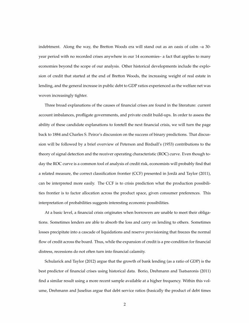
Figure 1 provides an overview of the incidence of financial crises in our data. The figure is

based on a sample of 14 advanced economies,4 which both in 1900 and 2000 comprised about

50% of world GDP according to Maddison (2005). Three features stand out in the figure. First,

it is clear that crises were relatively common up to the start of World War II. Second, from the

creation (in 1944) to the fall (in 1971) of the Bretton Woods system, there were no crises recorded

for our sample of countries. Thereafter, a number of isolated economies experienced financial

events of varying consequence. The end of the sample includes the recent financial storm, which

engulfed virtually every country in our sample.

Figure 1: The Incidence of Crises over Time

F‐1

Figure 1. The Incidence of Crises over Time

Notes: For any given year, the figure displays how many countries (out of a possible 14) are experiencing a financial crisis.

Notes: For any given year, the figure displays how many countries (out of a possible 14) are experiencing a financialcrisis. See text.

3 For a nice overview of Strong’s influence in shaping the international monetary system leading up to the GreatDepression see Ahamed (2009).

4 These are: Australia, Canada, Switzerland, Germany, Denmark, Spain, France, the U.K., Italy, Japan, the Nether-lands, Norway, Sweden and the U.S.

5

Since then, the prospects of sovereign default in Europe’s periphery have been added to the

fears of a banking collapse. The ”fiscal embarrassments of governments” we alluded to earlier

are another of the leading explanations for financial crises. Figure 2 displays the debt-to-GDP

ratios for our 14 economies broken down into a sample that excludes the U.S., and the U.S. series

on its own. U.S. government debt levels were very low (below 20 percent of GDP) leading up to

World War I, after which they temporarily doubled. They gradually declined thereafter and by

the dawn of the Great Depression they had nearly made up for the World War I effort. The debt-

to-GDP ratio climbed after the Great Depression, the result of large losses in economic activity

rather than to activist fiscal policy or the implementation of the social safety net mechanisms that

were to come.

Figure 2: Total Public Debt to GDP Ratio

F‐2

Figure 2. Public Debt to GDP Ratio

Notes: the figure displays debt-to-GDP ratios for the US and for the average of the remaining 13 countries in the sample.

Notes: The figure displays the U.S. and the average for the remaining 13 countries in the sample. See text.

The most defining feature of debt in our data is World War II. Debt levels climbed to 120

percent of GDP in the U.S. Once the war ended, debt levels were continuously reduced until the

mid-1970s, bottoming out at about 40 percent of GDP. That inflection point corresponds rather

6

curiously with the resumption of financial crises in our sample. But remember that debt had also

continually declined from the end of World War I up to the Great Depression. It is unclear from a

cursory look at the data where the debt needle is pointing to on the financial crisis causal-meter.

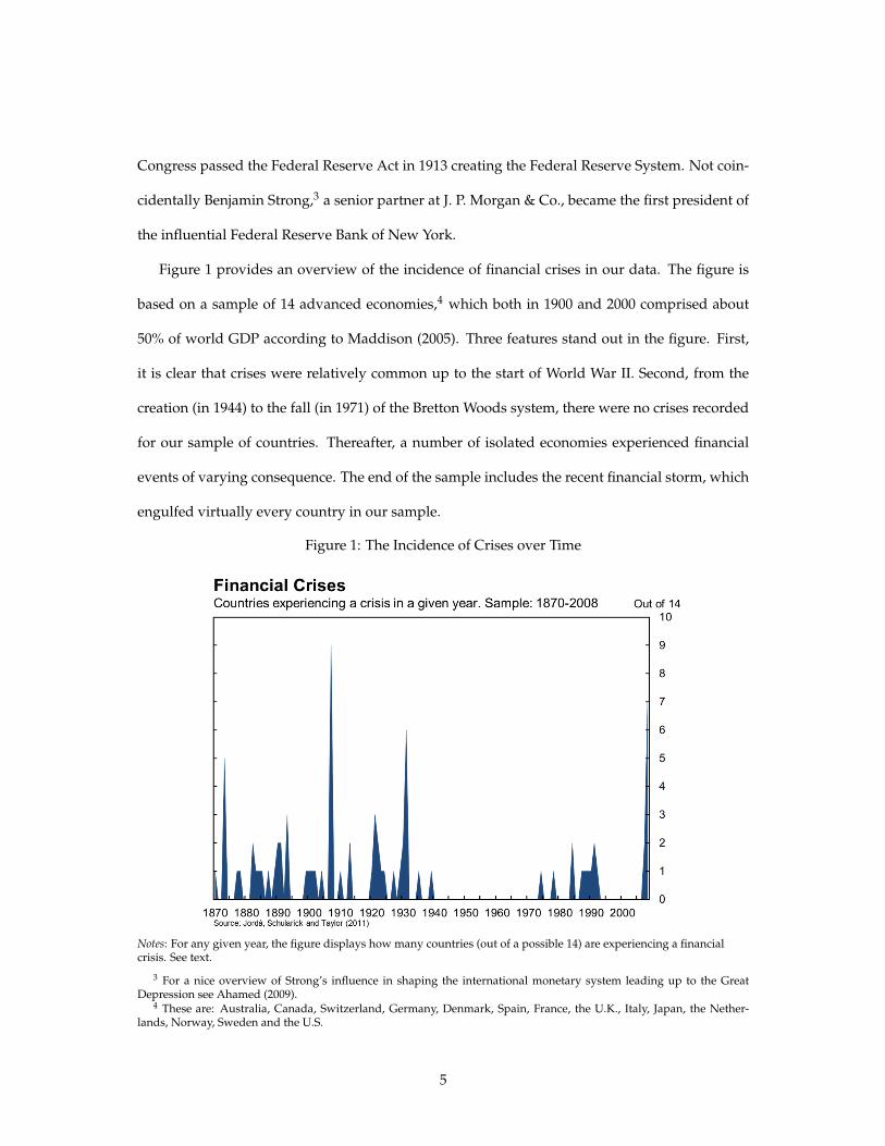
Although debt levels as a percent of GDP had been substantially higher in the average of

countries that excluded the U.S. in the pre-World War II era, thereafter the international expe-

rience seems more similar to the U.S. Debt levels began a steady climb in the 1970s with the

expansion of the welfare state, from about 40 percent to about 60 percent of GDP when the Great

Recession struck.

Figure 3: Current Account to GDP Ratio

F‐3

Figure 3. Current Account to GDP Ratio

Notes: the figure displays the current account for the U.S. and for the average of the remaining 13 countries in the sample.

Notes: The figure displays the average for the U.S. and the average for the remaining 13 countries in the sample. See text.

External imbalances are another oft cited suspect in the financial crisis mystery. Data on

current account balances as a percent of GDP are displayed in Figure 3. Again, the U.S. and the

average across the sample excluding the U.S. are displayed in tandem. Trends in the current

account are harder to discern than trends in debt with a few exceptions. The U.S. ran large

surpluses in World War I and at the end of World War II. The Bretton Woods era stands out

7

as a period in which imbalances were very moderate, perhaps not surprisingly. In addition to

fixed exchange rates, the Bretton Woods system imposed severe restrictions to capital mobility.

Starting in the mid-1970s as these restrictions became gradually undone, imbalances grew as a

percent of GDP. In the case of the U.S., they reached nearly 6 percent of GDP as the real estate

bubble hit its zenith, before the start of the Great Recession.

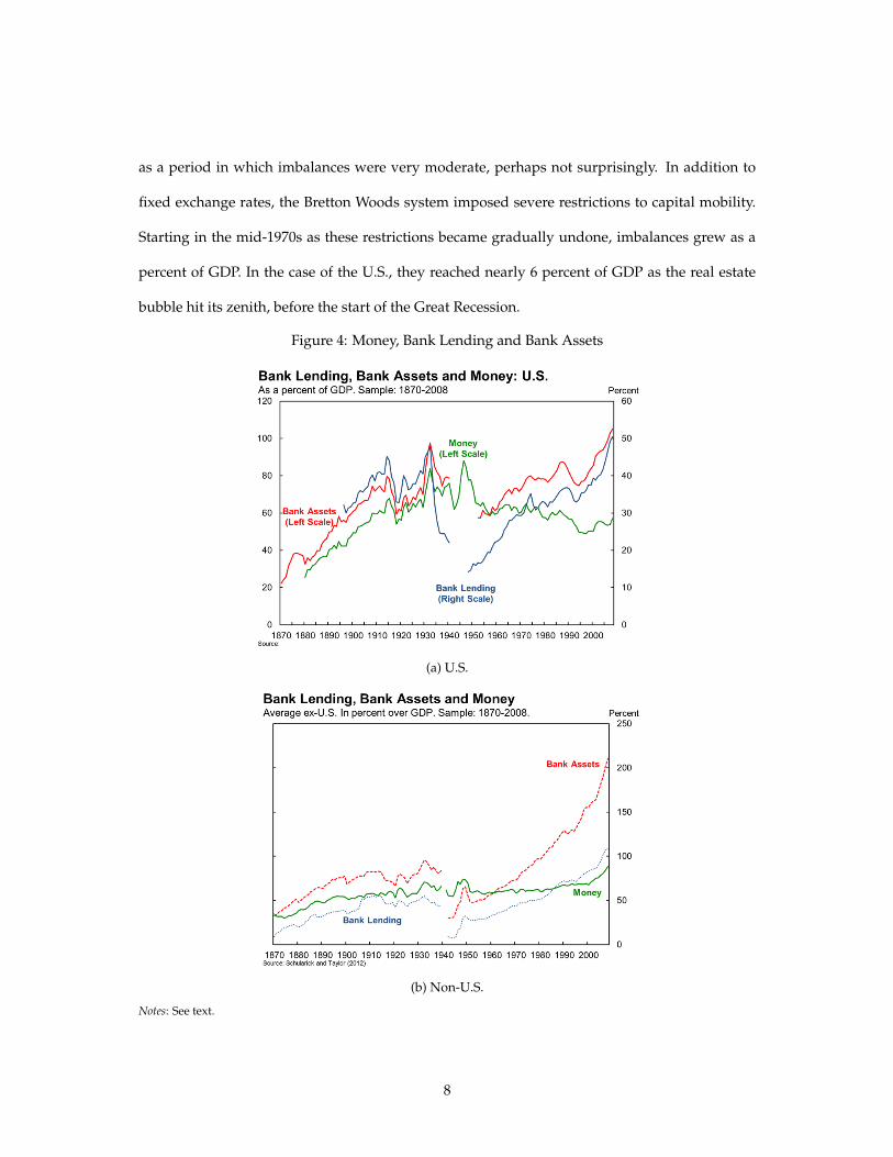
Figure 4: Money, Bank Lending and Bank Assets

F‐4

Figure 4. Money, Bank Lending and Bank Assets

Panel A: U.S.

Panel B: Average of remaining 13 countries

(a) U.S.

F‐4

Figure 4. Money, Bank Lending and Bank Assets

Panel A: U.S.

Panel B: Average of remaining 13 countries

(b) Non-U.S.

Notes: See text.

8

Schularick and Taylor (2012) document the fast rise of private credit after World War II, which

only accelerated further after the fall of Bretton Woods. Figure 4 displays how the tight link

between broad measures of money and bank lending broke down after World War II. The era

of money ushered in the era of credit. The figure displays a ”Money” variable (typically M2

or M3), ”Bank Lending” which refers to outstanding domestic loans, and ”Bank Assets” which

supplement bank lending with other assets held by banks such as Treasury securities, and so on.

Figure 5: Share of Real Estate Lending relative to Total Lending

F‐5

Figure 5. Share of Real Estate Lending in Bank Lending

Notes: See text.

Figure 5 provides a more detailed view of what may be behind this steep increase in lending.

It displays the ratio of real estate lending (commercial and by households) to total lending. For

the U.S., real estate lending was a relatively small share of total lending (under 15 percent) up

until the end of World War I. Thereafter the ratio climbed to 30 percent by the 1970s. In the short

span of the next 40 years, the ratio would double again to about 60 percent.

External imbalances, credit expansions and large capital financial flows are not independent

9

from one another. Often they reflect opposite sides of the same coin. And if our objective were to

assign a causal interpretation, it could be a daunting task to separate their independent effects.

Our objective is different, more pragmatic. Can these variables help us anticipate the next finan-

cial crisis? How can we can conceptualize the trade-offs involved in a policy designed to head-off

a crisis even if we mistakenly expect one to happen? The next section introduces a toolkit to think

more clearly about how this can be done.

3 Evaluating Predictions of Economic Episodes

3.1 Statistical Framework

There is a vast literature in econometrics dedicated to models of binary dependent models. This

section is not about finding which of these models provides a more accurate prediction. It is

about evaluating predictors and predictions themselves, and it is about presenting the trade-offs

associated with decisions based on these predictions. Denote yτ ∈ {0, 1} the binary indicator we

want to predict. If we are interested in predicting financial crises themselves, y may indicate if at

time τ a country is experiencing a crisis or not, for example. It could also refer to a classification

of recessions into financial and normal bins instead. The subindex k indicating the country in ykτ

is omitted to make the presentation more fluid.

Let the scalar xτ ∈ (−∞, ∞) denote the scoring classifier or classifier for short. This could be

a single predictor, an index based on several predictors, a probability forecast, and so on. The

definition of what is a classifier is quite general. What is important is that predictions yτ ∈

{0, 1} for yτ will be the result of the rule yτ = sign(xτ − c) where c ∈ (−∞, ∞). Note that the

implicit assumption here is that the larger xτ is, the more likely yτ = 1. Trivially, one can take

the negative of a given candidate classifier if the opposite is true. It should be clear that any

monotone transformation of xτ will not make the predictions any more accurate. Given the sign-

rule used to generate yτ , a monotone transformation simply scales c up or down accordingly.

10

The probabilities of success and failure associated with the prediction-outcome pair {yτ , yτ}

can be summarized by the following contingency table:

Prediction

Negative Positive

Outcome Negative TN(c) = P(yτ = 0|yτ = 0) FP(c) = P(yτ = 1|yτ = 0)

Positive FN(c) = P(yτ = 0|yτ = 1) TP(c) = P(yτ = 1|yτ = 1)

TN(c) denotes the true negative rate for a given threshold c. Recall that yτ = 0 if xτ < c so

that yτ is implicitly a function of c although it is not indicated explicitly to save on notation.

Similarly TP(c) denotes the true positive rate for a given threshold c. These are the rates of suc-

cessful predictions whose counterparts are FN(c) for false negatives and FP(c) for false positives

when the predictions are incorrect instead. Notice that by construction, TN(c) + FP(c) = 1 and

FN(c) + TP(c) = 1. In the statistics literature, TP(c) is sometimes called sensitivity, and TN(c)

specificity.

Notice that as c → ∞, TN(c) → 0 and TP(c) → 1 whereas if c → −∞ then TN(c) → 1

and TP(c) → 0. Thus, choosing the threshold c is like, say, choosing how much steel to allocate

between the production of forks (here TN(c) say) and knives (TP(c) in following the example).

Allocate more steel to producing knives (TP(c)) –that is, choose a larger value of c– and you will

produce less forks (TN(c)). But the better the technology (the better the classification ability),

the more of both can be produced with the same amount of steel, whichever the combination. In

economics, this is the familiar environment characterized by the production possibilities frontier.

Jorda and Taylor (2011) use this similarity to label the set of {TN(c), TP(c)} for all values of c as

the correct classification frontier (CCF). In statistics it is common to display the set of {TP(c), FP(c)}

for all values of c. That curve is the well-known receiver operating characteristics (ROC) curve.

The ROC curve is common in the biological and medical sciences for the purposes of assessing

11

medical diagnostic procedures, although its origin is in signal detection theory (Peterson and

Birdsall, 1953). Nowadays, ROC methods are well-established in statistics. Two worthwhile

monographs on the subject are Pepe (2003) and Zhou, Obuchowski and McClish (2011).

Consider our production possibilities frontier analogy one more time. The amount of input

optimally allocated to producing each good will depend on the relative demand for each good.

The optimal production mix is one in which technology is used to its potential and the share

produced of each good (the marginal rate of transformation) is determined by the marginal rate

of substitution between the goods. Peirce (1884) had a similar insight when considering the

accuracy of binary predictions. His ‘utility of the method’ is what we might call today expected

utility and when it refers to choosing the threshold c, it can be expressed as maximizing:

maxc

E(U(c)) = UpPTP(c)π + UnP (1− TP(c))π+ (1)

UpN(1− TN(c))(1− π) + UnNTN(c)(1− π)

where π = P(yτ = 1), that is, the unconditional probability of an event or a positive. The

notation UxX uses the lower case to denote the prediction and the uppercase to denote the actual,

where x ∈ {p, n} and X ∈ {P, N}. P, p stand for “positive” and N, n stand for “negative.”

Before discussing what the optimal choice of threshold c is, it may be useful to display graph-

ically the CCF against U(c) to discuss the features of the problem. This is done in Figure 6. We

say that a predictive technology yτ is uninformative for yτ if TP(c) = 1− TN(c), that is, one

cannot improve the correct classification rate for positives without diminishing the classification

rate for negatives by the exactly same amount. This is displayed in the figure as the diagonal

dotted line from the point [0, 1] to [1, 0]. Consider the other extreme, a situation in which the

predictive technology yτ perfectly classifies yτ . In that case we obtain the CCF corresponding to

the north-east corner of the unit-square. Typically we will be in the intermediate case between

these two extremes, displayed in the figure with the concave curve. The closer to the diagonal,

12

the worse the predictive technology.

Figure 6: The Correct Classification Frontier

F‐6

Figure 6. The Correct Classification Frontier

Notes: the dotted diagonal line refers to an uninformative classifier. The vertical distance between the CC Frontier in red and the dotted line is the Kolmogorov-Smirnov (KS) distance. The green north-east corner of the unit square is the perfect classifier. An example of indifference curves presented in orange. The tangent of the indifference curve to the correct classification frontier denotes the “optimal operating point.”

Notes: The dotted diagonal line refers to an uninformative classifier. The vertical distance between the CC frontier in redand the dotted line is the Kolmogorov-Smirnov (KS) distance. The green morth-east corner of the unit squarecorresponds to the perfect classifier. Example indifference curves are presented in orange. The tangent of theindifference curve to the correct classification frontier denotes ”optimal operating point.” See text.

Overlaid on the figure is a set of indifference curves. The closer the indifference curve to the

origin, the lower the utility. Since the CCF displays the highest correct classification rates for each

threshold c, optimality is achieved when the CCF is tangent to the indifference curve. We have

displayed an extreme case in which the policymaker has preferences weighed towards getting

accurate predictions of events (yτ = 1). Clearly, when the predictive technology yτ perfectly

classifies yτ , the relative preferences of one correct classification rate over the other do not matter

since we have a corner solution.

A few examples help understand the set up better. Suppose the policymaker values correct

classification of positives (say recessions) and negatives (expansions) equally and that he dis-

likes errors equally. Moreover, suppose he dislikes errors by the same amount he values correct

13

predictions. Further, suppose that the unconditional incidence of events (recessions in the exam-

ple) is π = 1/2. Indeed, lots of assumptions. Then the optimal threshold c is that point in the

CCF that has slope -1 since the relative marginal rate of substitution is also -1 in that case. This

point happens to maximize the distance between the CCF and the benchmark diagonal and is

displayed in Figure 6 with a ”KS.” The reason it is labeled KS is that it corresponds to the well

known Kolmogorov-Smirnov statistic

KS = maxc

∣∣∣∣2(TN(c) + TP(c)2

− 12

)∣∣∣∣ . (2)

The KS statistic maximizes the difference between the average correct classification rates of the

candidate predictive technology and the average correct classification rates of the benchmark

uninformative classifier. Since in the latter case TN(c) = 1− TP(c), then that average is simply

1/2 for any value of c. The difference is scaled by 2 so that KS ∈ [0, 1]. By construction, the KS

statistic also maximizes the Youden (1950) J index

J(c) = TP(c)− FP(c).

The Youden index is referred to as the ”science of the method” in Peirce (1884).

Other commonly reported statistics can be seen as special cases of the set-up in (1). For ex-

ample, by setting utility weights of 1 for correct calls and 0 for incorrect calls, one obtains and

accuracy rate

A(c) = TP(c)π + TN(c)(1− π)

whereas setting utility weights to 0 for correct calls and 1 for incorrect calls, one obtains the error

rate instead

E(c) = 1− A(c) = FN(c)π + FP(c)(1− π).

14

Moreover, it is easy to see that

A(c) =1 + J(c)

2; E(c) =

1− J(c)2

.

In general, π will not be 1/2 and the utility weights need not be constrained the way we have

described in the computation of KS, A(c) and E(c). Rather, the utility weights will depend on the

policymaker’s trade-offs in correctly diagnosing the appropriate policy stance, versus mistakes

of commission (implementing policy when it is not needed) or omission (failing to act when it

is needed). Using the set-up in expression (1), the optimal operating point (as is known in the

literature) and denoted c∗ is the point where

dTP(c)dTN(c)

∣∣∣∣c=c∗

= − (1− π)

π

(UnN −UpN)

(UpP −UnP). (3)

That is, the point were the marginal rate of transformation (in keeping with our analogy to the

production possibilities frontier) between TP(c) and TN(c) and the expected marginal rate of

substitution (given by the right hand side of (3)), equal each other.

We now have a good understanding of the building blocks of the problem at hand. Impor-

tantly, the statistical and economic layers of the problem critically interact with each other. Pref-

erences appear to play an important role. An the unconditional incidence of events, which we

denoted as π, also seems to matter. How then should one choose one classifier over another? Are

traditional metrics appropriate? As a way to set the stage for the next section, consider Figure 7.

Figure 7 displays two CCFs. One CCF is labeled ”A” and the other ”B.” CCFA clearly achieves

a higher value of the KS statistic than CCFB. On the other hand, the preferences of the policy-

maker, indicated by the indifference curves tangent to the CCFs, suggest that CCFB would allow

the policymaker to achieve a higher degree of utility. In this example, the policymaker cares

more about correctly calling expansions or negatives (yτ = 0) than recessions. The traditional

15

Figure 7: Which of Two CCFs is Preferable?

F‐7

Figure 7. Which of Two CCFs is Preferable?

Notes: The CCF labeled “A” and displayed in green has a higher KS value than the CCF labeled “B” and displayed in a dashed red line. However, preferences displayed by indifference curves in blue would suggest that classifier “B” is preferable to “A.”

True Positive Rate

True Negative Rate

Notes: The CCF labeled “A” and displayed in green has a higher KS value than the CCF labeled “B” and displayed in adashed red line. However, preferences displayed by indifference curves in blue would suggest that classifier “B” ispreferable to “A.” See text.

statistical metric (here based on the KS statistic) may an insufficient measure of what option is

preferable.

The basic point is self-evident by now. Consider one last example. Suppose that the un-

conditional incidence π = 0.05, a situation that will arise when evaluating rare events almost

definitionally. A prediction technology consisting in assigning yτ = 0 ∀τ will have a success

rate in predicting non-events of 100%. Typical measures of fit for binary models will therefore

have difficulty separating the performance of one model against another. In fact, the accuracy

rate defined earlier will be above 90% and the error rate below 10%. Clearly a better measure of

performance is needed. The next section provides one such measure.

3.2 The Area Under the Curve: AUC

Although the KS statistic relies on a number of empirically inconvenient assumptions, it has a

long tradition in statistics. At an intuitive level, the KS is a sensible measure of distance. It can be

thought of as the uniform distance between the empirical distribution of yτ when yτ = 0, versus

16

the empirical distribution of yτ when yτ = 1. The distribution of the KS statistic, although non-

standard, is well-understood. Nowadays, derivation of this distribution often relies on empirical

process theory (see e.g. Shorack and Wellner, 1986). Whenever a parametric model is used to

compute yτ , say by estimating a probit or a logit using a vector of covariates, its distribution will

change –an inconvenient feature.

In practice, the CCF summarizes the range of {TP, TN} choices for a given predictive tech-

nology. The better the prediction technology, the higher the TP rate for a given TN rate or vice

versa. And we know that the further from the uninformative classifier diagonal, the better. One

popular summary statistic of the CCF is to calculate the area under that curve or AUC.

Consider the uninformative classifier first, a diagonal bisecting the unit square. That classifier

obviously has an AUC = 1/2. The CCF for the perfect classifier hugs the north-east corner of the

unit square, as we saw in Figure 6, and hence has an AUC = 1. Typical empirical CCFs will have

an AUC in-between. The closer to 1, the better the classifier, the closer to 0.5, the worse.

The AUC is easy to calculate empirically using non-parametric methods. Given a sample of

M observations, let M0 indicate the number of observations for which yτ = 0, and let M1 denote

the number of observations for which yτ = 1 instead, with M = M0 + M1. Moreover, let{

vj}M0

j=1

denote the classifier xτ when yτ = 0 and let {ui}M1i=1 denote the classifier xτ when yτ = 1. Then

AUC =1

M0M1∑∀v

∑∀u

Υ (v, u) (4)

where Υ(v, u) = 1 if v < u, Υ(v, u) = 0 if v > u and Υ(v, u) = 1/2 if v = u.

Under standard regularity assumptions, Hsieh and Turnbull (1996) use empirical process the-

ory and show that√

M(

AUC− P(v < u))→ N(0, σ2). (5)

The formula for the variance term σ2 is provided in that paper. Hanley and McNeil (1982) and

Obuchowski (1994) provide a convenient approximation for σ2 using the interpretation of the

17

AUC as a Mann-Whitney U-statistic. DeLong, DeLong and Clarke-Pearson (1988) provide a

more general formula that is available in the statistical packages SAS and STATA. Jackknife and

bootstrap procedures are also available (see Pepe, 2003 and references therein).

Asymptotic normality of the AUC is very convenient for inference, specially when compared

to the KS statistic. Several features must be kept in mind, however. First a predictive technology

A stochastically dominates a technology B if CCFA > CCFB uniformly over some region, and

CCFA = CCFB otherwise. However, AUCA > AUCB does not necessarily imply this condition.

As Figure 7 showed, AUCA > AUCB but CCFA < CCFB over some region, which happened to

be the relevant region to the policymaker in that example. Our applications do not display this

feature so we will be content with comparing AUCs. For a more expansive discussion of how

to deal with crossing CCFs and appropriate inferential procedures for that case, the reader is

referred to Jorda and Taylor (2011).

4 Recessions, Financial Crises and the Role of Credit

Credit buildups have been identified as a predictor of financial crises by Claessens, Kose and Ter-

rones (2011); Borio, Drehmann and Tsatsaronis (2012) and Schularick and Taylor (2012) among

others. However, Gadea-Rivas and Perez-Quiros (2012), henceforth denoted GRPQ, dispute

these findings. They argue that there is considerable uncertainty in determining when the re-

cession will come. Therefore, sorting whether a recession is financial in nature or not given

knowledge of when the recession strikes, provides the analyst with undue advantage and is un-

realistic in a real-time policy setting. GRPQ show that credit has little predictive ability if one

removes that advantage.

This section investigates these issues in more detail. The first step is to examine the basic

findings in the literature regarding the role of credit in sorting recessions into “financial” or “nor-

mal.” Thus, the dependent variable is defined over the sample of recession periods only, and

18

takes the value of 1 whenever the recession is financial, 0 if it is not. That is, the frequency of the

data is event-time. Next, the objective is to investigate the claims in GRPQ. Here the objective is

to sort the data into expansions and recessions at a yearly frequency rather than in event-time.

The third and final experiment, also at a yearly frequency rather than in event-time, directly

examines whether financial crises can be predicted in a policy-relevant time-scale. That is, the

dependent variable takes the value of 1 whenever there is a recession tied to a financial crisis,

and 0 otherwise. Thus, the 0 category includes “normal” recessions and expansions.

The data for the analysis consists of a subset of the data in Jorda, Schularick and Taylor (2011)

and Schularick and Taylor (2012), extended with data for debt-to-GDP ratios through a larger

and ongoing research effort.5 A detailed description is available in the references. Here I provide

a broad description of the salient features.

The sample reaches back to 1870 and ends in 2008. Observations are available at a yearly fre-

quency for 14 advanced economies. These countries are: Australia, Canada, Japan, Austria, Den-

mark, France, Germany, Italy, the Netherlands, Norway, Spain, Sweden, the U.K. and the U.S. For

each country data on expansions, recessions and financial crises are borrowed from Jorda, Schu-

larick and Taylor (2011).6 Then I consider three potential classifiers: the current account balance,

expressed as a ratio to GDP, the public debt to GDP ratio, and the ratio of bank loans to GDP as a

measure of private credit. In addition, data on long-term government debt interest rates (usually

with a maturity of about 5 years) is used as a proxy for the debt service ratio when interacted

with debt measures, whether public or private. Absent data on private debt, government debt

interest rates are the best we can do. Although it is possible that the spread between private and

government yields varies over the business cycle, the hope is that this variation is small relative

to the level effects.5 This research effort is funded with a grant from the Institute of New Economic Thinking and consists of a consider-

able data collection and processing effort by coauthors, Moritz Schularick and Alan Taylor, and a small army of researchassistants.

6 Briefly, the classification of recessions as financial blends financial episodes identified by Reinhart and Rogoff (2009)with episodes identified by Laeven and Valencia (2008). It then identifies a recession as “financial” if a financial crisistakes place within a two year window

19

Sometimes data are not available from the beginning of the sample. As a result and de-

pending on the candidate classifier, the sample varies from over 1,550 to over 1,350 country-year

observations when determining whether a particular year is classified as an expansion or a re-

cession. When the objective is to sort recessions into financial or normal recessions, the sample

ranges from 204 to 160 country-recession observations. World War I and II are excluded from the

sample.

4.1 Financial versus Normal Recessions

The goal of this section is to replicate the basic finding in Schularick and Taylor (2012), among

others, that credit buildups during expansions predict the likelihood of financial crisis. Consider

three indicators often used for this purpose: (1) the accumulated growth in the current account

to GDP ratio over the expansion (Current Account); (2) the accumulated growth in bank lending

as a ratio of GDP over the expansion (Private Credit); and (3) the accumulated growth of public

debt as a ratio of GDP during the expansion (Public Debt). In addition, I also consider interacting

(2) and (3) with the 5-year government bond interest rate to calculate an approximate measure

of burden as in Drehmann and Juselius (this volume). I call these respectively Private Burden

and Public Burden. Finally, I also consider the combination of (1)-(3), which I call Joint and the

combination when Private Credit and Public Debt are interacted with the 5-year government

bond rate. I call this variable Joint Burden. Notice that the frequency of the data is event-time: it is

conditioned on there being a recession. Notice also that the indicators contain information prior

to the beginning of the recession but not after.

When considered singly, there is no need to specify a model relating each of the indicators and

the dependent variable, in this case, a dummy variable that takes the value of 1 if the recession

is “financial,” 0 if it is “normal.” One of the features of the CCF and the AUC is that their value

remains unchanged by monotone transformations of the classifier. This is a useful feature: the

value of the classifier does not depend on the modeling skills of the analyst.

20

Although a model is not necessary to investigate classifiers one at a time, it is when more than

one classifier is considered. There are many modeling options available. Here I assume that the

log-odds ratio of the financial/normal recession conditional probabilities are a linear function of

the classifiers so that

logP [ykτ = 0|Xkτ−1]

P [ykτ = 1|Xkτ−1]= β0 + β′Xkτ−1 (6)

where the index k refers to the country and Xkτ−1 refers to a vector of classifiers observed be-

fore the τ recession starts. This is a popular model for classification in statistics and with a

long-standing tradition in economics, the logit model. Hastie, Tibshirani and Friedman (2009)

recommend such a specification as a matter of empirical practice. Notice that expression (6) does

not allow for fixed effects. The reason is that in the subsample analysis (to be discussed shortly),

some of the countries did not experience a financial crisis. Therefore, including a fixed effect

would leave no variability in the data to identify the effect of Xkτ−1. Another reason to exclude

fixed effects is that in a model with no classifiers, fixed effects would generate a null AUC above

0.5. Knowledge of the average recessions that are financial across countries would be informa-

tive.

Robustness checks include two modifications. First, results for the full sample and the pre-

and post-World War II eras are calculated. The motivation was discussed earlier in light of Figure

4. Second, the appendix replicates the results reported in Table 1 using fixed effects estimators.

This robustness check confirms that the relative ranking of the classifiers discussed below re-

mains the same, only the AUC values attained are slightly higher, as would be expected.

21

Table 1: Classifying recessions into financial or normal

(a) Full SampleClassifier AUC SE 95% Conf. Interval N. Obs

Current Account 0.49 0.05 [0.40, 0.59] 204Private Credit 0.61∗∗ 0.05 [0.50, 0.72] 184Private Burden 0.61∗∗ 0.05 [0.50, 0.71] 184Public Debt 0.52 0.05 [0.43, 0.62] 196Public Burden 0.52 0.05 [0.43, 0.61] 194Joint 0.64∗∗ 0.06 [0.53, 0.75] 160Joint Burden 0.61∗∗ 0.06 [0.50, 0.72] 160

(b) Pre-WWII SampleClassifier AUC SE 95%Conf. Interval N. Obs

Current Account 0.49 0.06 [0.38, 0.61] 136Private Credit 0.54 0.07 [0.42,0.67] 118Private Burden 0.56 0.07 [0.43, 0.69] 118Public Debt 0.53 0.06 [0.42, 0.65] 130Public Burden 0.54 0.06 [0.43, 0.65] 128Joint 0.62∗ 0.07 [0.49, 0.76] 100Joint Burden 0.61∗ 0.07 [0.47, 0.74] 100

(c) Post-WWII SampleClassifier AUC SE 95% Conf. Interval N. Obs

Current Account 0.48 0.09 [0.31, 0.65] 68Private Credit 0.82∗∗ 0.07 [0.69, 0.95] 66Private Burden 0.78∗∗ 0.08 [0.62, 0.93] 66Public Debt 0.48 0.08 [0.31, 0.64] 66Public Burden 0.54 0.08 [0.38, 0.71] 66Joint 0.84∗∗ 0.05 [0.74, 0.95] 60Joint Burden 0.79∗∗ 0.07 [0.64, 0.93] 60The data are in event time and refer to recession episodes identified by Jorda, Schularick and Taylor (2011) using the Bryand Boschan (1971) algorithm. The classification into “financial” and “normal” is explained in Jorda, Schularick andTaylor (2011). It is largely based on Reinhart and Rogoff (2009) and Laeven and Valencia (2008). The analysis precludesfixed effects as explained in the text. The appendix replicates the table using fixed effects. The number of observationsvaries due to differences in data availability across classifiers. Current Account refers to the accumulated current accountbalance in the preceding expansion as a ratio to GDP. Private Credit refers to the accumulated growth in bank lendingduring the preceding expansion, as a ratio to GDP. Private Burden interacts Private Credit with the 5-year governmentbond rate. Public Debt refers to the accumulated growth in public debt as a ratio to GDP in the preceding expansion.Public Burden interacts Public Debt with the 5-year government debt interest rate. Joint combines the previous classifiersin a logit model and Joint Burden also combines variables but with Private Credit and Public Debt interacted with the5-year government bond interest rate. ∗p < 0.10, ∗∗p < 0.05. See text.

22

Table 1 reports the results of this analysis, which by and large confirm what the literature has

reported. Panel (a) in the table refers to the full sample and shows that the variables based on

measures of the accumulated growth in private credit have significant (albeit a low AUC of 0.61)

classification ability relative to all the others, which are not significant. When the variables are

combined together, the AUC increases to 0.64, a very slight improvement.

Panels (b) and (c) in Table 1 break down the sample at World War II. In the pre-WWII era,

private credit remains the most relevant variable but even its classification ability is no better

than a coin toss. There are some gains from combining the private and public data, with an AUC

that is about 0.62 and significant. However, the post-WWII era tells a somewhat different story.

Here the role of credit buildups is very clear. Private credit achieves an AUC of around 0.8, highly

significant and much closer to the ideal value of 1. Meanwhile, the alternative classifiers attain

very low AUCs, as we saw earlier. Using private and public data improves the AUC somewhat

but the results are clearly driven by what happens with private credit rather than public debt.

As an illustration, Figure 8 displays the CCFs for each of the cases considered, that is, when

variables (1)-(3) are used singly and the their combination. The top panel displays the CCF using

the full sample and the bottom panel displays the CCFs using the post-WWII sample. These

CCFs are direct non-parametric estimates of the combinations {TP(c), TN(c)} calculated over

different values of the threshold c. Smoother CCFs can be obtained by using parametric models,

such as the binormal model (see, e.g., Pepe, 2003). Figure 8 is meant to show that CCFs are

straightforward to calculate.

23

Figure 8: Nonparametric Estimates of the CCF

AUC = 0.49 (0.05) AUC = 0.61 (0.05)

AUC = 0.61 (0.06) AUC = 0.52 (0.05)

0.00

0.25

0.50

0.75

1.00

0.00

0.25

0.50

0.75

1.00

0.00 0.25 0.50 0.75 1.000.00 0.25 0.50 0.75 1.00

Current Account Private Credit

Joint Public Debt

Tru

e P

ositi

ve R

ate

True Negative Rate

(a) Full Sample

AUC = 0.48 (0.09) AUC = 0.82 (0.07)

AUC = 0.79 (0.07) AUC = 0.54 (0.08)

0.00

0.25

0.50

0.75

1.00

0.00

0.25

0.50

0.75

1.00

0.00 0.25 0.50 0.75 1.000.00 0.25 0.50 0.75 1.00

Current Account Private Credit

Joint Public Debt

Tru

e P

ositi

ve R

ate

True Negative Rate

(b) Post-WWII Sample

Notes: Each chart displays the CCF for a particular classifier along with the value of the AUC and its standard error (in

parenthesis). Estimates of the AUC correspond to those reported in Table 1. The diagonal line represents the null CCF of

no classification ability. The top panel based on the full sample, the bottom panel based on post-WWII data only. See

text.

24

4.2 Expansions versus Recessions

The results of the previous section suggest that the more credit builds up during the expansion,

the more probable the subsequent recession will be financial in nature. GRPQ argue that this

result is of little practical relevance: Predicting when the next recession will happen is very dif-

ficult anyway. Obsessive control of credit may snuff economic growth unnecessarily. Or in the

parlance of Peirce, there would be too many false positives if authorities constantly responded

to credit buildups. This section examines this proposition. Moving from event-time to calendar-

time, the question is whether any of the indicators exploited in the previous section would help

predict whether a recession is likely happen in a given year. Instead of using the indicators mea-

sured over the expansion, since that information is unavailable a priori, I examine 5-year moving

averages to smooth over cyclical fluctuations and get a sense of medium run build-ups of stress.

Table 2 reports the results of this exercise, which by and large confirm GRPQ. Using the full

sample, panel (a) shows that neither private lending nor private debt (or the related “burden”

measures) appear to have much classification ability, although used jointly, the AUC attains a

value of 0.59. This value is relatively low, but statistically different from the coin toss null. Inter-

estingly, the current account balance has similar classification ability, with an AUC of 0.58. Panels

(b) and (c) in Table 2 breakdown the analysis by era. Panel (b) focuses on the pre-WWII sample,

whereas panel (c) focuses on the post-WWII period. Unlike the previous section, the subsample

analysis delivers similar results to the full sample results reported in panel (a).

25

Table 2: Sorting Expansions and Recessions


Current Account 0.58∗∗ 0.02 [0.54, 0.61] 1559Private Credit 0.52 0.02 [0.48, 0.55] 1468Private Burden 0.53∗ 0.02 [0.50, 0.57] 1462Public Debt 0.51 0.02 [0.47, 0.54] 1534Public Burden 0.50 0.02 [0.47, 0.54] 1521Joint 0.59∗∗ 0.02 [0.55, 0.62] 1351Joint Burden 0.59∗∗ 0.02 [0.55, 0.62] 1351


Current Account 0.57∗∗ 0.02 [0.52, 0.61] 744Private Credit 0.52 0.02 [0.47,0.56] 661Private Burden 0.52 0.02 [0.47, 0.56] 655Public Debt 0.50 0.02 [0.45, 0.54] 727Public Burden 0.50 0.02 [0.45, 0.54] 716Joint 0.59∗ 0.02 [0.54, 0.63] 579Joint Burden 0.59∗ 0.02 [0.54, 0.64] 579


Current Account 0.62∗∗ 0.03 [0.56, 0.68] 815Private Credit 0.51 0.03 [0.44, 0.57] 807Private Burden 0.51 0.03 [0.45, 0.58] 807Public Debt 0.56∗ 0.03 [0.49, 0.62] 805Public Burden 0.55∗ 0.03 [0.49, 0.62] 805Joint 0.61∗∗ 0.03 [0.55, 0.68] 772Joint Burden 0.61∗∗ 0.03 [0.54, 0.67] 772The data are at yearly frequency. Recessions and expansions determined by Jorda, Schularick and Taylor (2011) usingthe Bry and Boschan (1971) algorithm. The analysis precludes fixed effects as explained in the text. The appendixreplicates the table using fixed effects. The number of observations varies due to differences in data availability acrossclassifiers. Classifiers calculated as 5-five year moving averages. Current Account refers to the current account balance asa ratio to GDP. Private Credit refers to bank lending as a ratio to GDP. Private Burden interacts Private Credit with the5-year government bond rate. Public Debt refers to public debt as a ratio to GDP. Public Burden interacts Public Debt withthe 5-year government debt interest rate.Joint combines the previous classifiers in a logit model and Joint Burden alsocombines variables but with Private Credit and Public Debt interacted with the 5-year government bond interest rate.∗p < 0.10, ∗∗p < 0.05. See text.

26

4.3 Detecting Financial Recessions Only

The final experiments reported in this section are an attempt to reconcile the results discussed

in sections 4.1 and 4.2. Can we discriminate recessions enveloped in financial distress from any

other event, be it a typical recession of a period of expansion? The answer is reported in Table 3.

Table 3: Financial Recessions against the Rest


Current Account 0.59∗∗ 0.03 [0.54, 0.64] 1559Private Credit 0.60∗∗ 0.03 [0.54, 0.66] 1468Private Burden 0.59∗ 0.03 [0.53, 0.65] 1462Public Debt 0.52 0.03 [0.47, 0.58] 1534Public Burden 0.52 0.03 [0.47, 0.58] 1521Joint 0.67∗∗ 0.03 [0.61, 0.72] 1351Joint Burden 0.61∗∗ 0.03 [0.55, 0.67] 1351


Current Account 0.57∗∗ 0.03 [0.51, 0.62] 744Private Credit 0.61∗∗ 0.03 [0.55, 0.67] 661Private Burden 0.62∗ 0.03 [0.56, 0.68] 655Public Debt 0.53 0.03 [0.46, 0.59] 727Public Burden 0.52 0.03 [0.46, 0.59] 716Joint 0.67∗∗ 0.03 [0.60, 0.73] 579Joint Burden 0.66∗∗ 0.03 [0.60, 0.73] 579


Current Account 0.70∗∗ 0.05 [0.61, 0.80] 815Private Credit 0.78∗∗ 0.06 [0.66, 0.90] 807Private Burden 0.79∗ 0.06 [0.67, 0.92] 807Public Debt 0.57 0.08 [0.42, 0.72] 805Public Burden 0.60 0.08 [0.45, 0.75] 805Joint 0.80∗∗ 0.06 [0.69, 0.92] 772Joint Burden 0.79∗∗ 0.07 [0.66, 0.92] 772The data are at yearly frequency. Recessions and expansions determined by Jorda, Schularick and Taylor (2011) usingthe Bry and Boschan (1971) algorithm. The analysis precludes fixed effects as explained in the text. The appendixreplicates the table using fixed effects. The number of observations varies due to differences in data availability acrossclassifiers. Classifiers calculated as 5-five year moving averages. Current Account refers to the current account balance asa ratio to GDP. Private Credit refers to bank lending as a ratio to GDP. Private Burden interacts Private Credit with the5-year government bond rate. Public Debt refers to public debt as a ratio to GDP. Public Burden interacts Public Debt withthe 5-year government debt interest rate. Joint combines the previous classifiers in a logit model and Joint Burden alsocombines variables but with Private Credit and Public Debt interacted with the 5-year government bond interest rate.∗p < 0.10, ∗∗p < 0.05. See text.

Consider panel (a) in the table first. Here the role of private lending and the current account

appear to have resurrected somewhat, with AUCs of about 0.60 and statistically significant. Us-

ing the classifiers jointly, the AUC improves even more to a respectable 0.67 even though public

27

debt on its own appears to be no better than the toss of a coin. The subsample analysis is es-

pecially revealing here. Whereas results using the pre-WWII sample and reported in panel (b)

of Table 3, are very similar to the full sample results in panel (a), the story is quite different in

the post-WWII sample. Panel (c) of Table 3 clearly suggests that bank lending can be a very use-

ful indicator, with an AUC of about 0.8, closer to the ideal value of 1. Notice that combining

information does nothing to improve classification ability since the AUC remains at about 0.80.

5 Conclusion

Evaluating competing statistical models of events rarely observed is difficult. Because events

are observed infrequently, one requires long samples to gain enough variability to identify the

trigger factors. In addition, because the unconditional probabilities of observing an event are

low, traditional metrics fail to select the model that provides the best economic advantage. This

paper presents some solutions in the context of predicting financial crises. The novelty of these

solutions is that they bring statistical as well as economic principles in unified fashion.

In good times, private credit is viewed as subsidiary to explaining fluctuations in macroeco-

nomic aggregates. Despite an extensive collection of theoretical models in which credit plays a

role in amplifying fluctuations of the cycle, the literature has found scant support for this role

empirically. No doubt this reflects, at least in part, the difficulties in isolating the independent

effect of credit channels from more traditional and well understood monetary channels.

The elementary analysis of the business cycle provided here reinforces typical findings in the

literature. Growth in private credit does not appear to foretell the next recession much better

than random chance. How much public debt increases relative to GDP turns out to be a just as

poor an indicator although somewhat improved since WWII.

These results collide with a more recent literature on the role of credit in financial crises. In

fact, when one conditions on a recession taking place, private credit emerges as an important

28

sorting variable of when a recession is likely to turn into a financial crisis. To a large extent, this

result is driven by the post-WWII sample and the era of financialization.

The pieces start to fall into place. In the post-World War II experience the Bretton-Woods era

of stringent capital controls emerges as an oasis of financial calm. Whether it was due to stronger

regulation, fiscal rebalancing following the war effort, or entirely different reasons, we need to

understand better why the Bretton Woods period stands alone in the history of the last 140 years.

The end of Bretton-Woods saw a variety of new trends develop, from governments carrying

higher debt burdens to a veritable explosion of credit at an international level. And in recent

times, real-estate lending has taken over as the primary purpose of bank lending. Credit may

not explain the run-of-the mill recessions but it can explain when recessions turn into financial

crises. Complementary evidence from Jorda, Schularick and Taylor (2012) indicates that once the

recession breaks out, regardless of its cause, higher levels of private credit accumulation during

the expansion make the recovery slower.

If the goal is to single out periods of turmoil from all others, the role of credit comes to the

fore once again. And once again its relevance seems mostly driven by the experience of the post-

WWII era. We do not yet understand the role that credit plays in the economy well, but we

understand well enough that monitoring credit closely appears to be a worthwhile enterprise.

References

Ahamed, Liaquat. 2009. The Lords of Finance: The Bankers Who Broke the World. The PenguinPress: New York.

Bernanke, Ben S. and Mark Gertler. 1989. Agency Costs, Net Worth, and Business Fluctua-tions. American Economic Review 79(1):Ta 14-31.

Bernanke, Ben S. and Mark Gertler. 1995. Inside the Black Box: The Credit Channel of Mon-etary Policy Transmission. Journal of Economics Perspectives 9(4): 27-48.

Bernanke, Ben S., Mark Gertler and Simon Gilchrist. 1999. The Financial Accelerator in aQuantitative Business Cycle Framework. In Handbook of Macroeconomics, Vol. 1C, ed. JohnB. Taylor and Michael Woodford, 1341-93, Vol. 15. Amsterdam: Elsevier, North-Holland.

Claessens, Stijn, M. Ayhan Kose and Marco Terrones. 2011. Financial Cycles: What? How?When? Center for Economic Policy Research, Discussion Paper 8379.

29

DeLong, Elizabeth R., David M. DeLong and Daniel L. Clarke-Pearson. 1988. Comparingthe Areas under Two of More Correlated Receiver Operating Characteristic Curves: A Non-parametric Approach. Biometrics 44: 837-845.

Drehmann, Mathias, Claudio Borio and Kostas Tsatsaronis. 2011. Anchoring Countercycli-cal Capital Buffers: The Role of Credit Aggregates. International Journal of Central Banking7(4): 189-240.

Drehmann, Mathias and Mikael Juselius. 2013. Evaluating EWIs for banking crises – satis-fying policy requirements. International Journal of Forecasting, this issue.

Gadea Rivas, Marıa Dolores and Gabriel Perez Quiros. 2012. The Failure to Predict theGreat Recession. The Failure of Academic Economics? A View Focusing on the Role ofCredit. CEPR working paper 9269.

Granger, Clive W. J. and Mark J. Machina. 2006. Forecasting and Decision Theory. In Hand-book of Economic Forecasting. Graham Elliott, Clive W. J. Granger and Allan Timmermann(eds). Amsterdam: Elsevier, North-Holland.

Hanley, James A. and Barbara J. McNeil. 1982. The Meaning and Use of the Area Under theReceiver Characteristic (ROC) Curve. Radiology 143: 29-36.

Hastie, Trevor, Robert Tibshirani and Jerome Friedman. 2009. The Elements of StatisticalLearning: Data Mining, Inference and Prediction, 2nd edition. Springer: New York.

Hsieh, Fushing and Bruce W. Turnbull. 1996. Nonparametric and Semiparametric Estima-tion of the Receiver Operating Characteristic Curve. Annals of Statistics 24: 25-40.

Jorda, Oscar, Moritz Schularick and Alan M. Taylor. 2011. Financial Crises, credit boomsand external imbalances: 140 years of lessons. IMF Economic Review 59(2): 340-378.

Jorda, Oscar, Moritz Schularick and Alan M. Taylor. 2012. When Credit Bites Back: Lever-age, Business Cycles and Crises. NBER working paper 17621.

Jorda, Oscar and Alan M. Taylor. 2011. Performance Evaluation of Zero Net-InvestmentStrategies. NBER working paper 17150.

Maddison, Angus. 2005. Measuring and Interpreting World Economic Performance 1500-2001. The Review of Income and Wealth 51(1): 1-35.

Mitchell, Wesley C. 1927. Business cycles: the problem and its setting. National Economic Bu-reau of Economic Research: New York.

Obuchowski, Nancy A. 1994. Computing Sample Size for Receiver Operating CharacteristicCurve Studies. Investigative Radiology 29(2): 238-243.

Peirce, Charles S. (1884). The Numerical Measure of the Success of Predictions. Science, 4:453-454.

Pepe, Margaret S. 2003. The Statistical Evaluation of Medical Tests for Classification and Predic-tion. Oxford University Press: Oxford, U.K.

Peterson, W. Wesley and Theodore G. Birdsall. 1953. The Theory of Signal Detectability: PartI. The General Theory. Electronic Defense Group, Technical Report 13, June 1953. Availablefrom EECS Systems Office, University of Michigan.

30

Schularick, Moritz and Alan M. Taylor. 2012. Credit Booms Gone Bust: Monetary Policy,Leverage Cycles and Financial Crises, 1870-2008. American Economic Review 102(2): 1029-61.

Shorack, Galen R. and Jon A. Wellner. 1986. Empirical Processes with Applications to Statistics.John Wiley & Sons: New Jersey.

Youden, W. J. 1950. Index for Rating Diagnostic Tests. Cancer 3: 32-35.

Zhou, Xia-Hua, Nancy A. Obuchowski and Donna K. McClish. 2011. Statistical Methods inDiagnostic Medicine, 2nd Edition. John Wiley & Sons: New Jersey.

31

Appendix

Financial Crises versus Normal Recessions: Fixed Effects Estimates

This section replicates the results in Table 1, section 4.1, but allowing for fixed effects.

Table A1: Classifying recessions into financial or normal: Fixed Effects Estimates(a) Full Sample

Classifier AUC SE 95% Conf. Interval N. ObsCurrent Account 0.62∗∗ 0.05 [0.54, 0.71] 204Private Credit 0.66∗∗ 0.05 [0.57, 0.76] 184Private Burden 0.66∗∗ 0.05 [0.57, 0.75] 184Public Debt 0.66∗∗ 0.04 [0.57, 0.74] 196Public Burden 0.65∗∗ 0.04 [0.57, 0.74] 194Joint 0.71∗∗ 0.05 [0.62, 0.75] 160Joint Burden 0.70∗∗ 0.05 [0.60, 0.81] 160

(b) Pre-WWII SampleClassifier AUC SE 95% Conf. Interval N. Obs

Current Account 0.63∗∗ 0.05 [0.52, 0.73] 136Private Credit 0.65∗∗ 0.06 [0.54,0.76] 118Private Burden 0.65∗∗ 0.06 [0.54, 0.76] 118Public Debt 0.67∗∗ 0.05 [0.56, 0.78] 130Public Burden 0.66∗∗ 0.05 [0.55, 0.77] 128Joint 0.70∗∗ 0.06 [0.58, 0.82] 97Joint Burden 0.69∗∗ 0.06 [0.57, 0.81] 97


Current Account 0.72∗∗ 0.09 [0.55, 0.89] 49Private Credit 0.92∗∗ 0.06 [0.81, 1] 47Private Burden 0.81∗∗ 0.08 [0.65, 0.96] 47Public Debt 0.72∗∗ 0.09 [0.55, 0.89] 47Public Burden 0.74∗∗ 0.09 [0.56, 0.91] 47Joint 0.99∗∗ 0.01 [0.97, 1] 43Joint Burden 0.89∗∗ 0.05 [0.79, 1] 43The data are in event time and refer to recession episodes identified by Jorda, Schularick and Taylor (2011) using the Bryand Boschan (1971) algorithm. The classification into “financial” and “normal” is explained in Jorda, Schularick andTaylor (2011). It is largely based on Reinhart and Rogoff (2009) and Laeven and Valencia (2008). The analysis precludesfixed effects as explained in the text. The appendix replicates the table using fixed effects. The number of observationsvaries due to differences in data availability across classifiers. Current Account refers to the accumulated current accountbalance in the preceding expansion as a ratio to GDP. Private Credit refers to the accumulated growth in bank lendingduring the preceding expansion, as a ratio to GDP. Private Burden interacts Private Credit with the 5-year governmentbond rate. Public Debt refers to the accumulated growth in public debt as a ratio to GDP in the preceding expansion.Public Burden interacts Public Debt with the 5-year government debt interest rate. Joint combines the previous classifiersin a logit model and Joint Burden also combines variables but with Private Credit and Public Debt interacted with the5-year government bond interest rate. ∗p < 0.10, ∗∗p < 0.05. See text.

32

Expansions v. Recessions: Fixed Effects Estimates


Table A2: Sorting Expansions and Recessions: Fixed Effects Estimates(a) Full Sample



Current Account 0.64∗∗ 0.02 [0.60, 0.68] 744Private Credit 0.62∗∗ 0.02 [0.58, 0.67] 661Private Burden 0.62∗∗ 0.02 [0.58, 0.67] 655Public Debt 0.60∗∗ 0.02 [0.56, 0.64] 727Public Burden 0.60∗∗ 0.02 [0.56, 0.64] 716Joint 0.68∗∗ 0.02 [0.63, 0.72] 579Joint Burden 0.68∗∗ 0.02 [0.63, 0.72] 579


Current Account 0.66∗∗ 0.03 [0.61, 0.72] 815Private Credit 0.60∗∗ 0.03 [0.55, 0.66] 807Private Burden 0.61∗∗ 0.03 [0.56, 0.67] 807Public Debt 0.64∗ 0.03 [0.59, 0.70] 805Public Burden 0.64∗ 0.03 [0.59, 0.70] 805Joint 0.67∗∗ 0.03 [0.61, 0.72] 772Joint Burden 0.67∗∗ 0.03 [0.61, 0.72] 772The data are at yearly frequency. Recessions and expansions determined by Jorda, Schularick and Taylor (2011) usingthe Bry and Boschan (1971) algorithm. The analysis includes fixed effects as explained in the text. The appendixreplicates the table using fixed effects. The number of observations varies due to differences in data availability acrossclassifiers. Classifiers calculated as 5-five year moving averages. Current Account refers to the current account balance asa ratio to GDP. Private Credit refers to bank lending as a ratio to GDP. Private Burden interacts Private Credit with the5-year government bond rate. Public Debt refers to public debt as a ratio to GDP. Public Burden interacts Public Debt withthe 5-year government debt interest rate. Joint combines the previous classifiers in a logit model and Joint Burden alsocombines variables but with Private Credit and Public Debt interacted with the 5-year government bond interest rate.∗p < 0.10, ∗∗p < 0.05. See text.

33

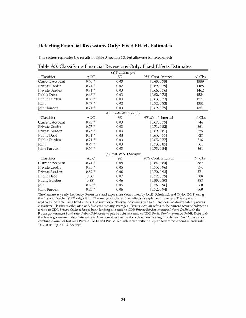
Detecting Financial Recessions Only: Fixed Effects Estimates


Table A3: Classifying Financial Recessions Only: Fixed Effects Estimates(a) Full Sample



Current Account 0.73∗∗ 0.03 [0.67, 0.79] 744Private Credit 0.77∗∗ 0.03 [0.71, 0.82] 661Private Burden 0.75∗∗ 0.03 [0.69, 0.81] 655Public Debt 0.71∗∗ 0.03 [0.65, 0.77] 727Public Burden 0.71∗∗ 0.03 [0.65, 0.77] 716Joint 0.79∗∗ 0.03 [0.73, 0.85] 561Joint Burden 0.79∗∗ 0.03 [0.73, 0.84] 561


Current Account 0.74∗∗ 0.05 [0.64, 0.84] 582Private Credit 0.85∗∗ 0.05 [0.75, 0.96] 574Private Burden 0.82∗∗ 0.06 [0.70, 0.93] 574Public Debt 0.66∗ 0.07 [0.52, 0.79] 588Public Burden 0.68∗ 0.06 [0.55, 0.80] 588Joint 0.86∗∗ 0.05 [0.76, 0.96] 560Joint Burden 0.83∗∗ 0.06 [0.72, 0.94] 560The data are at yearly frequency. Recessions and expansions determined by Jorda, Schularick and Taylor (2011) usingthe Bry and Boschan (1971) algorithm. The analysis includes fixed effects as explained in the text. The appendixreplicates the table using fixed effects. The number of observations varies due to differences in data availability acrossclassifiers. Classifiers calculated as 5-five year moving averages. Current Account refers to the current account balance asa ratio to GDP. Private Credit refers to bank lending as a ratio to GDP. Private Burden interacts Private Credit with the5-year government bond rate. Public Debt refers to public debt as a ratio to GDP. Public Burden interacts Public Debt withthe 5-year government debt interest rate. Joint combines the previous classifiers in a logit model and Joint Burden alsocombines variables but with Private Credit and Public Debt interacted with the 5-year government bond interest rate.∗p < 0.10, ∗∗p < 0.05. See text.

34

assessing the historical role of credit: business cycles ... · assessing the historical role of...

Documents