at SciVerse ScienceDirect

Journal of Environmental Management 127 (2013) S132eS144

Contents lists available

Journal of Environmental Management

journal homepage: www.elsevier .com/locate/ jenvman

Assessing spatial uncertainties of land allocation using a scenarioapproach and sensitivity analysis: A study for land use in Europe

Peter H. Verburg a,*, Andrzej Tabeau b, Erez Hatna c

a Institute for Environmental Studies and Amsterdam Global Change Institute, VU University Amsterdam, The NetherlandsbAgricultural Economics Research Institute - LEI /International policy, The Hague, The NetherlandscCenter for Advanced Modeling, Department of Emergency Medicine, The Johns Hopkins University, Baltimore, MD, USA

a r t i c l e i n f o

Article history:Received 19 February 2012Received in revised form14 August 2012Accepted 30 August 2012Available online 29 September 2012

Keywords:Spatial uncertaintyScenario approachSensitivity analysisLand useLand cover

* Corresponding author. Tel.: þ31 (0)20 59 83594.E-mail address: Peter.Verburg@vu.nl (P.H. Verburg

0301-4797/$ e see front matter � 2012 Elsevier Ltd.http://dx.doi.org/10.1016/j.jenvman.2012.08.038

a b s t r a c t

Land change model outcomes are vulnerable to multiple types of uncertainty, including uncertainty ininput data, structural uncertainties in the model and uncertainties in model parameters. In coupledmodel systems the uncertainties propagate between the models. This paper assesses uncertainty ofchanges in future spatial allocation of agricultural land in Europe as they arise from a general equilibriummodel coupled to a spatial land use allocation model. Two contrasting scenarios are used to capture someof the uncertainty in the development of typical combinations of economic, demographic and policyvariables. The scenario storylines include different measurable assumptions concerning scenario specificdrivers (variables) and parameters. Many of these assumptions are estimations and thus include a certainlevel of uncertainty regarding their true values. This leads to uncertainty within the scenario outcomes.In this study we have explored how uncertainty in national-level assumptions within the contrastingscenario assumptions translates into uncertainty in the location of changes in agricultural land use inEurope. The results indicate that uncertainty in coarse-scale assumptions does not translate intoa homogeneous spread of the uncertainty within Europe. Some regions are more certain than others infacing specific land change trajectories irrespective of the uncertainty in the macro-level assumptions.The spatial spread of certain and more uncertain locations of land change is dependent on locationconditions as well as on the overall scenario conditions. Translating macro-level uncertainties touncertainties in spatial patterns of land change makes it possible to better understand and visualize theland change consequences of uncertainties in model input variables.

� 2012 Elsevier Ltd. All rights reserved.

1. Introduction

Integrated environmental assessments of socio-ecologicalsystems generally suffer from high levels of uncertainty. Commu-nication of such uncertainties is important and is increasinglyreceiving academic attention, especially because such uncertaintiesmay influence the perception of risks and effectiveness of mitiga-tion and adaptation measures related to global change (Adger et al.,2009; Pidgeon and Fischhoff, 2011; Polasky et al., 2011). Someuncertainties may be reduced by more and better observation data,improvedmodels andmore attention for calibration and validation.However, it is clear that major uncertainties will remain in large-scale environmental assessments as a result of our incompleteknowledge and data of the socio-ecological system, strong simpli-fications in model representations and the inherent uncertainty of

).

All rights reserved.

socio-economic and political developments. A complicating factorof the assessment of uncertainties in environmental research is thefact that many impacts are location specific: environmental changeaffects locations in different ways and also the uncertainty inassessment results is spatially variable. Most uncertainty analysis inenvironmental assessment have focussed on the uncertainty inaggregate model results and lack a representation of the spatialvariability of such uncertainties (Tebaldi et al., 2005). Spatialassessments of uncertainties have mainly been made for static dataor physical models (Heuvelink et al., 2010; Nol et al., 2010) andmuch less in integrated scenario studies. Representing the spatialvariation of global change impacts is critical in designing adapta-tion measures and in the communication of global changeprocesses (Hulme, 2008). Local impacts can differ considerablyfrom the average global impact; consequently localities may notrecognize themselves in the average numbers (Hulme, 2010). In thetranslation of global environmental change to more local impacts itis, therefore, important to also address the spatial aspects of theuncertainty. This paper will present an analysis of the propagation

P.H. Verburg et al. / Journal of Environmental Management 127 (2013) S132eS144 S133

of uncertainty in global scalemodels of land use change; translatinguncertainty in aggregate drivers of land change to spatial uncer-tainties in the occurrence of land change processes within Europe.

On a global scale, allocation of agricultural land and foodproduction is largely determined by socio-economic driving forcessuch as macro-economic growth, demographic development andtechnical progress. However, agricultural production is onlypossible in geographic areas having suitable biophysical and socio-economic characteristics. Since socio-economic and biophysicaldrivers of land change operate across different spatial and temporalscales (Overmars and Verburg, 2006; Turner et al., 2007) the spatialallocation of agro-food production and related land use have scale-dependent uncertainties.

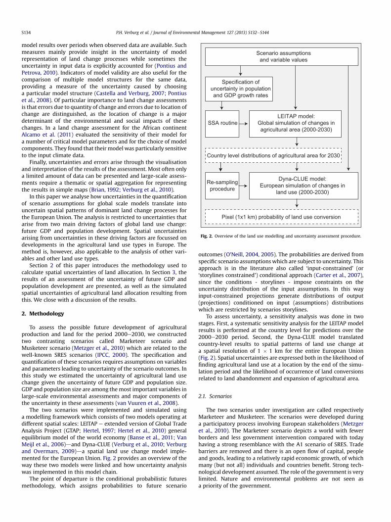
Numerous classification schemes for the sources of uncertaintyin environmental assessments have been introduced, and it is notalways possible to reconcile the different taxonomies. Matott et al.(2009), Refsgaard et al. (2007) and Walker (2003) provide over-views of the different uncertainties in integrated environmentalassessment and list methods to address these uncertainties. Wewill not attempt to classify the different uncertainties in inte-grated environmental assessments in a generic manner, nor beexhaustive in our inventory of all possible sources of uncertainty.Instead, we focus on providing a short overview of the differenttypes of uncertainty as these occur in a typical analysis of land usechange at a broad spatial scale. Fig. 1 presents the typical steps ofsuch an assessment with its associated uncertainties (Rounsevellet al., 2006; Schaldach et al., 2011; Verburg et al., 2006). Landchange assessments often start from a number of storylines orscenarios in which the uncertainties in possible socio-economicand political development are made explicit through defininga series of, internally consistent, narratives. Many of the narrativesused in assessments are variations of the well-known SRESstorylines (IPCC, 2000) inwhich the storylines are organized alongthe range of possible developments in respectively the level ofglobal integration and the level of governance on environmentaland equity issues (Busch, 2006; Metzger et al., 2010; Westhoeket al., 2006). To be able to simulate such scenarios in quantita-tive models a further specification and elaboration of thescenarios is needed, often following the so-called Story-And-Simulation approach (Alcamo, 2008, 2009). The storylines are in

Scenario storyline

Specification of scenarioassumptions

Data and dataprocessing

Quantitative modelling

Representation and interpretationof modelling results

Uncertainty in world

development

Personal judgement

and assumptions

Uncertainty in observations

and bias due to processing

Incomplete knowledge,

simplification and

representation errors

Visualisation and interpretation

methods, judgement

Fig. 1. Typical sequence of land change assessments and associated sources ofuncertainty.

this step translated to quantitative estimates of the main driversand exogenous variables of the simulation model. These quanti-fied drivers as well as other data are used in the simulation model.Many models of land change are available (see overviews of Priessand Schaldach (2008) and Verburg et al. (2004)). For large-scaleassessments a combination of coarse-grained global models,which deal with the macro-level dynamics betweenworld regionsand countries, and more detailed spatial allocation models iscommon (Rounsevell et al., 2006; Verburg et al., 2008). In a finalstep selected results are presented and interpreted, often aftera reduction of the information through spatial and thematicaggregation to manage the large amount of information resultingfrom these models (Verburg et al., 2010).

These different steps are subject to different types of uncer-tainties and require different methods for assessment. The firststeps of the assessments, the specification and quantification of thescenario narratives are in itself a means of dealing with theinherent uncertainty of future socioeconomic and technologyconditions and the uncertainty in the policy environment (Mosset al., 2010). Busch (2006) analysed existing Europe-widescenario studies and compared the results of different approachesthat translate globally defined SRES storylines into detailedassessments of European land change. Different approaches for thesame scenario resulted for Western Europe in large differences infuture land use/cover changes ranging from moderate decreases(15%) to large increases (30%) in agricultural area depending on theassumptions about global trade, increase in agricultural produc-tivity and biofuel production that were made. Differences in theseassumptions originated from variations in the interpretation of theglobal storylines. In addition, also the differences in modellingapproach (which inherently refers to assumptions about systemfunction) were causing some of the observed differences. Differ-ences in interpretation and quantification of storylines is furtherexplored by Metzger et al. (2010) who explore how alternativeworldviews influence the interpretation of scenario outcomes andthereby the specification of input variables of models that simulatethe consequences of these scenarios. The authors propose todetermine a band-width of scenario outcomes based on thedifferences in personal judgement of the scenario interpretations.This band-width is determined by the range between the so-calledHigh-Expectation World (HEW) and Low-Expectation World(LEW). Similarly, Van Asselt and Rotmans (1996) use cultural theoryto analyse how different perceptions of reality and policy prefer-ences influence model routes in integrated assessment modelling,while focussing on population development and climate issues.

Another source of uncertainty is related to the input data.Integrated assessments of land change require a large amount ofinput data, representing current land use, socio-economic andbiophysical conditions. All these data are subject to thematic andspatial uncertainties. A good representation of land use data isa major challenge. Uncertainties depend on thematic representa-tion, scale, and the specific land use type (Fritz et al., 2011; Nol et al.,2008; Verburg et al., 2011). Dendoncker et al. (2008) analysed theuncertainties in land allocation patterns that arise from differentspatial rasterization methods of the initial land use data and thespatial resolution of these data. The authors compared the uncer-tainties originating from these differences in data representation tovariations in land change over a period of 50 years in 4 differentscenarios for the territory of Luxembourg. Differences between thespatial rasterization methods were at least as large as the differ-ences between the different scenarios.

Specifically for land change assessments Pontius et al. (2004)has proposed a range of methods that allow comparison ofspatially explicit modelling results with observed data. Thesemethods are targeted at providing measures of the validity of

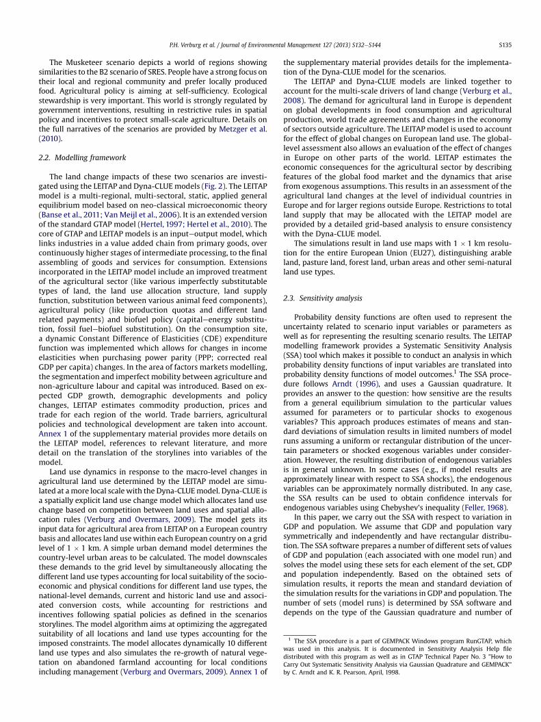
Scenario assumptionsand variable values

Specification ofuncertainty in populationand GDP growth rates

LEITAP model:Global simulation of changes inagricultural area (2000-2030)

SSA routine

Country level distributions of agricultural area for 2030

Dyna-CLUE model:European simulation of changes in

land use (2000-2030)

Re-samplingprocedure

Pixel (1x1 km) probability of land use conversion

Fig. 2. Overview of the land use modelling and uncertainty assessment procedure.

P.H. Verburg et al. / Journal of Environmental Management 127 (2013) S132eS144S134

model results over periods when observed data are available. Suchmeasures mainly provide insight in the uncertainty of modelrepresentation of land change processes while sometimes theuncertainty in input data is explicitly accounted for (Pontius andPetrova, 2010). Indicators of model validity are also useful for thecomparison of multiple model structures for the same data,providing a measure of the uncertainty caused by choosinga particular model structure (Castella and Verburg, 2007; Pontiuset al., 2008). Of particular importance to land change assessmentsis that errors due to quantity of change and errors due to location ofchange are distinguished, as the location of change is a majordeterminant of the environmental and social impacts of thesechanges. In a land change assessment for the African continentAlcamo et al. (2011) evaluated the sensitivity of their model fora number of critical model parameters and for the choice of modelcomponents. They found that their model was particularly sensitiveto the input climate data.

Finally, uncertainties and errors arise through the visualisationand interpretation of the results of the assessment. Most often onlya limited amount of data can be presented and large-scale assess-ments require a thematic or spatial aggregation for representingthe results in simple maps (Brian, 1992; Verburg et al., 2010).

In this paper we analyse how uncertainties in the quantificationof scenario assumptions for global scale models translate intouncertain spatial patterns of dominant land change processes forthe European Union. The analysis is restricted to uncertainties thatarise from two main driving factors of global land use change:future GDP and population development. Spatial uncertaintiesarising from uncertainties in these driving factors are focussed ondevelopments in the agricultural land use types in Europe. Themethod is, however, also applicable to the analysis of other vari-ables and other land use types.

Section 2 of this paper introduces the methodology used tocalculate spatial uncertainties of land allocation. In Section 3, theresults of an assessment of the uncertainty of future GDP andpopulation development are presented, as well as the simulatedspatial uncertainties of agricultural land allocation resulting fromthis. We close with a discussion of the results.

2. Methodology

To assess the possible future development of agriculturalproduction and land for the period 2000e2030, we constructedtwo contrasting scenarios called Marketeer scenario andMusketeer scenario (Metzger et al., 2010) which are related to thewell-known SRES scenarios (IPCC, 2000). The specification andquantification of these scenarios requires assumptions on variablesand parameters leading to uncertainty of the scenario outcomes. Inthis study we estimated the uncertainty of agricultural land usechange given the uncertainty of future GDP and population size.GDP and population size are among themost important variables inlarge-scale environmental assessments and major components ofthe uncertainty in these assessments (van Vuuren et al., 2008).

The two scenarios were implemented and simulated usinga modelling framework which consists of two models operating atdifferent spatial scales: LEITAP e extended version of Global TradeAnalysis Project (GTAP; Hertel, 1997; Hertel et al., 2010) generalequilibrium model of the world economy (Banse et al., 2011; VanMeijl et al., 2006)dand Dyna-CLUE (Verburg et al., 2010; Verburgand Overmars, 2009)da spatial land use change model imple-mented for the European Union. Fig. 2 provides an overview of theway these two models were linked and how uncertainty analysiswas implemented in this model chain.

The point of departure is the conditional probabilistic futuresmethodology, which assigns probabilities to future scenario

outcomes (O’Neill, 2004, 2005). The probabilities are derived fromspecific scenario assumptionswhich are subject to uncertainty. Thisapproach is in the literature also called ‘input-constrained’ (or‘storylines constrained’) conditional approach (Carter et al., 2007),since the conditions - storylines - impose constraints on theuncertainty distribution of the input assumptions. In this wayinput-constrained projections generate distributions of output(projections) conditioned on input (assumptions) distributionswhich are restricted by scenarios storylines.

To assess uncertainty, a sensitivity analysis was done in twostages. First, a systematic sensitivity analysis for the LEITAP modelresults is performed at the country level for predictions over the2000e2030 period. Second, the Dyna-CLUE model translatedcountry-level results to spatial patterns of land use change ata spatial resolution of 1 � 1 km for the entire European Union(Fig. 2). Spatial uncertainties are expressed both in the likelihood offinding agricultural land use at a location by the end of the simu-lation period and the likelihood of occurrence of land conversionsrelated to land abandonment and expansion of agricultural area.

2.1. Scenarios

The two scenarios under investigation are called respectivelyMarketeer and Musketeer. The scenarios were developed duringa participatory process involving European stakeholders (Metzgeret al., 2010). The Marketeer scenario depicts a world with fewerborders and less government intervention compared with todayhaving a strong resemblance with the A1 scenario of SRES. Tradebarriers are removed and there is an open flow of capital, peopleand goods, leading to a relatively rapid economic growth, of whichmany (but not all) individuals and countries benefit. Strong tech-nological development assumed. The role of the government is verylimited. Nature and environmental problems are not seen asa priority of the government.

1 The SSA procedure is a part of GEMPACK Windows program RunGTAP, whichwas used in this analysis. It is documented in Sensitivity Analysis Help filedistributed with this program as well as in GTAP Technical Paper No. 3 ”How toCarry Out Systematic Sensitivity Analysis via Gaussian Quadrature and GEMPACK”by C. Arndt and K. R. Pearson, April, 1998.

P.H. Verburg et al. / Journal of Environmental Management 127 (2013) S132eS144 S135

The Musketeer scenario depicts a world of regions showingsimilarities to the B2 scenario of SRES. People have a strong focus ontheir local and regional community and prefer locally producedfood. Agricultural policy is aiming at self-sufficiency. Ecologicalstewardship is very important. This world is strongly regulated bygovernment interventions, resulting in restrictive rules in spatialpolicy and incentives to protect small-scale agriculture. Details onthe full narratives of the scenarios are provided by Metzger et al.(2010).

2.2. Modelling framework

The land change impacts of these two scenarios are investi-gated using the LEITAP and Dyna-CLUEmodels (Fig. 2). The LEITAPmodel is a multi-regional, multi-sectoral, static, applied generalequilibrium model based on neo-classical microeconomic theory(Banse et al., 2011; Van Meijl et al., 2006). It is an extended versionof the standard GTAP model (Hertel, 1997; Hertel et al., 2010). Thecore of GTAP and LEITAP models is an inputeoutput model, whichlinks industries in a value added chain from primary goods, overcontinuously higher stages of intermediate processing, to the finalassembling of goods and services for consumption. Extensionsincorporated in the LEITAP model include an improved treatmentof the agricultural sector (like various imperfectly substitutabletypes of land, the land use allocation structure, land supplyfunction, substitution between various animal feed components),agricultural policy (like production quotas and different landrelated payments) and biofuel policy (capitaleenergy substitu-tion, fossil fuelebiofuel substitution). On the consumption site,a dynamic Constant Difference of Elasticities (CDE) expenditurefunction was implemented which allows for changes in incomeelasticities when purchasing power parity (PPP; corrected realGDP per capita) changes. In the area of factors markets modelling,the segmentation and imperfect mobility between agriculture andnon-agriculture labour and capital was introduced. Based on ex-pected GDP growth, demographic developments and policychanges, LEITAP estimates commodity production, prices andtrade for each region of the world. Trade barriers, agriculturalpolicies and technological development are taken into account.Annex 1 of the supplementary material provides more details onthe LEITAP model, references to relevant literature, and moredetail on the translation of the storylines into variables of themodel.

Land use dynamics in response to the macro-level changes inagricultural land use determined by the LEITAP model are simu-lated at amore local scalewith the Dyna-CLUEmodel. Dyna-CLUE isa spatially explicit land use change model which allocates land usechange based on competition between land uses and spatial allo-cation rules (Verburg and Overmars, 2009). The model gets itsinput data for agricultural area from LEITAP on a European countrybasis and allocates land use within each European country on a gridlevel of 1 � 1 km. A simple urban demand model determines thecountry-level urban areas to be calculated. The model downscalesthese demands to the grid level by simultaneously allocating thedifferent land use types accounting for local suitability of the socio-economic and physical conditions for different land use types, thenational-level demands, current and historic land use and associ-ated conversion costs, while accounting for restrictions andincentives following spatial policies as defined in the scenariosstorylines. The model algorithm aims at optimizing the aggregatedsuitability of all locations and land use types accounting for theimposed constraints. The model allocates dynamically 10 differentland use types and also simulates the re-growth of natural vege-tation on abandoned farmland accounting for local conditionsincluding management (Verburg and Overmars, 2009). Annex 1 of

the supplementary material provides details for the implementa-tion of the Dyna-CLUE model for the scenarios.

The LEITAP and Dyna-CLUE models are linked together toaccount for the multi-scale drivers of land change (Verburg et al.,2008). The demand for agricultural land in Europe is dependenton global developments in food consumption and agriculturalproduction, world trade agreements and changes in the economyof sectors outside agriculture. The LEITAPmodel is used to accountfor the effect of global changes on European land use. The global-level assessment also allows an evaluation of the effect of changesin Europe on other parts of the world. LEITAP estimates theeconomic consequences for the agricultural sector by describingfeatures of the global food market and the dynamics that arisefrom exogenous assumptions. This results in an assessment of theagricultural land changes at the level of individual countries inEurope and for larger regions outside Europe. Restrictions to totalland supply that may be allocated with the LEITAP model areprovided by a detailed grid-based analysis to ensure consistencywith the Dyna-CLUE model.

The simulations result in land use maps with 1 � 1 km resolu-tion for the entire European Union (EU27), distinguishing arableland, pasture land, forest land, urban areas and other semi-naturalland use types.

2.3. Sensitivity analysis

Probability density functions are often used to represent theuncertainty related to scenario input variables or parameters aswell as for representing the resulting scenario results. The LEITAPmodelling framework provides a Systematic Sensitivity Analysis(SSA) tool which makes it possible to conduct an analysis in whichprobability density functions of input variables are translated intoprobability density functions of model outcomes.1 The SSA proce-dure follows Arndt (1996), and uses a Gaussian quadrature. Itprovides an answer to the question: how sensitive are the resultsfrom a general equilibrium simulation to the particular valuesassumed for parameters or to particular shocks to exogenousvariables? This approach produces estimates of means and stan-dard deviations of simulation results in limited numbers of modelruns assuming a uniform or rectangular distribution of the uncer-tain parameters or shocked exogenous variables under consider-ation. However, the resulting distribution of endogenous variablesis in general unknown. In some cases (e.g., if model results areapproximately linear with respect to SSA shocks), the endogenousvariables can be approximately normally distributed. In any case,the SSA results can be used to obtain confidence intervals forendogenous variables using Chebyshev’s inequality (Feller, 1968).

In this paper, we carry out the SSA with respect to variation inGDP and population. We assume that GDP and population varysymmetrically and independently and have rectangular distribu-tion. The SSA software prepares a number of different sets of valuesof GDP and population (each associated with one model run) andsolves the model using these sets for each element of the set, GDPand population independently. Based on the obtained sets ofsimulation results, it reports the mean and standard deviation ofthe simulation results for the variations in GDP and population. Thenumber of sets (model runs) is determined by SSA software anddepends on the type of the Gaussian quadrature and number of

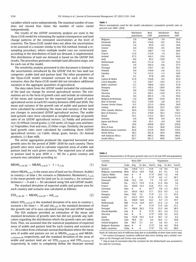
Table 1Macro assumptions used for the model calculations; cumulative growth rates inpercent over 2001e2030.

Marketeerpopulation

RealGDP

Musketeerpopulation

RealGDP

Belgium 5.9 106.3 �3.9 26.0Denmark 8.5 114.0 �0.2 35.4Germany 3.4 85.9 �6.2 18.6Greece 6.4 110.6 �4.5 30.0Spain 3.1 140.7 �7.4 30.0France 11.6 115.0 1.4 26.1Ireland 27.3 143.1 15.9 54.9Italy �0.6 85.2 �10.9 7.5Netherlands 18.2 111.4 2.5 32.5Austria 2.9 105.2 �6.6 27.5Portugal 6.4 110.7 �4.5 30.1Finland 6.0 110.0 �2.6 32.3Sweden 7.4 112.2 �1.3 34.0UK 9.1 97.8 �0.9 28.2Cyprus & Malta 21.9 134.8 6.5 43.4Czech Republic 1.5 150.7 �14.5 37.3Baltic countries �2.7 198.9 �18.2 57.0Hungary �5.7 145.5 �20.9 30.9Poland 6.0 176.8 �10.6 47.4Slovenia 3.3 105.1 �12.8 27.5Slovakia 9.4 201.5 �7.6 59.4Bulgaria & Romania �3.4 340.1 �23.0 81.6Rest of Europe 12.2 119.0 �2.8 25.3Former Soviet Union �0.1 215.3 �20.4 54.9Turkey 45.5 293.9 23.5 128.7USA, Canada, Mexico 26.4 113.0 24.3 58.7Rest of America 33.1 179.9 36.3 116.2Brazil 33.1 172.2 36.3 111.4Oceania 6.4 99.4 8.4 41.6Japan and Korea �0.9 63.1 �2.0 18.8China 10.6 430.8 20.2 239.9Rest of Asia 28.1 319.2 30.8 210.9Mediterranean countries 62.6 215.9 56.0 139.5North Africa 58.3 291.8 56.0 190.6Sub-Saharan Africa 82.7 405.2 98.8 184.2South-Africa 82.7 281.3 98.8 129.0

Table 2Statistical characteristics of 30 years growth rates (in %) of real GDP and population.

Country Real GDP Population

Name Code Avg. St. dev. Var(%) Avg. St. dev. Var(%)

Austria Aut 118.0 17.7 15.0 7.6 0.6 8.4Belgium, Luxemburg Belu 101.2 14.9 14.8 6.1 0.1 1.8Cyprus, Malta Euis # # 17.5a 24.0 1.2 4.9Czech Republic Cze # # 17.5a 4.2 1.1 26.7Denmark Dnk 72.2 5.4 7.5 7.8 0.7 9.4Finland Fin 121.7 13.9 11.4 11.5 0.4 3.6France Fra 104.0 12.5 12.0 15.3 1.2 7.7Germany Deu # # 10.7b 5.6 1.2 20.9Greece Grc 103.5 18.3 17.7 23.3 0.3 1.2Hungary Hun 76.0 7.2 17.5a �2.1 1.1 23.5Ireland Irl 312.7 35.7 11.4 27.1 1.0 3.8Italy Ita 104.9 14.9 14.2 6.7 1.3 19.7Netherlands Nld 111.6 12.0 10.7 21.2 1.2 5.8Poland Pol # # 17.5a 17.5 2.6 15.1Portugal Prt 166.6 28.3 17.0 15.3 4.4 28.5Slovak Republic Svk # # 17.5a 18.1 2.4 13.3Slovenia Svn # # 17.5a 14.9 2.2 14.5Spain Esp 132.8 16.5 12.4 18.7 1.2 6.2Sweden Swe 78.9 3.5 4.4 10.5 1.1 10.8United Kingdom Gbr 90.7 3.7 4.1 5.6 0.3 5.7Bulgaria, Romania Apeu # # 17.5a 5.6 4.4 78.8Baltic countries Euba # # 17.5a 5.6 4.5 80.9

Hash (#) indicates lack of sufficient data due to availability of short time series only.a For eastern European countries sufficient data were lacking and a similar vari-

ation as for Portugal and Greece was assumed.b Due to lack of consistent data the variation for the Netherlands was assumed to

be valid for Germany.

P.H. Verburg et al. / Journal of Environmental Management 127 (2013) S132eS144S136

variables which varies independently. Themaximal number of runsdoes not exceed four times the number of varies variedindependently.

The results of the LEITAP sensitivity analysis are used in theDyna-CLUEmodel for estimating the spatial consequences and landchange patterns of the estimated uncertainties at the level ofcountries. The Dyna-CLUE model does not allow the uncertaintiesto be assessed in a manner similar to the SSA method. Instead a re-sampling procedure, where multiple model runs are constructedaccording to the distribution of land use demand, is implemented.This distribution of land use demand is based on the LEITAP SSAresults. The procedure generates multiple land allocationmaps, onefor each run of the model.

The sensitivity analysis presented in this document is limited tothe uncertainties introduced by the LEITAP SSA for two land usecategories: arable land and pasture land. The other parameters ofthe Dyna-CLUE model remained constant for each of the twoscenarios, thus the Dyna-CLUE model did not introduce additionalvariation in the aggregate quantities of agricultural.

The data taken from the LEITAP model included the estimationof the land use change for several agricultural sectors. The esti-mations are in the form of growth rates and include an estimationof the mean and variance for the expected land growth of eachagricultural sector in each EU country between 2000 and 2030. Themean and variance of the growth rate of arable and pasture landwere calculated by combining the mean and variance of the landuse changes in associated LEITAP agricultural sectors. The arableland growth rates were calculated as weighted average of growthrates of six LEITAP agricultural sectors: (a) Paddy and processedrice; (b)Wheat, Cereal grains; (c) Oil seeds; (d) Sugar cane and beet;(e) Vegetables, fruit and nuts, (f) Other crops. Similarly, the pastureland growth rates were calculated by combining three LEITAPagricultural sectors: (a) Cattle, sheep, goats, horses; (b) Animalproducts; (c) Raw milk.

The sector aggregation produced the expected harvested areagrowth rates for the period of 2000e2030 for each country. Thesegrowth rates were used to calculate expected areas of arable andpasture land for each given country. The expected area of arableor pasture land in year 2030 (t ¼ 30) for a given country andscenario was calculated according to:

MEANc;s;lu;30 ¼ MEANc;s;lu;0 ��1þ rc;s;lu

�(1)

where MEANc,s,lu,t is the mean area of land use lu˛{Pasture, Arable}in country c at time t, for scenario s˛{Marketeer, Musketeer}, rc,s,luis the mean growth rate for land use lu, in country c, for scenario sbetween t ¼ 0 and t ¼ 30 calculated using SSA and LEITAP model.

The standard deviation of expected arable and pasture area foreach country and scenario was calculated as follows:

STDc;s;lu;30 ¼ MEANc;s;lu;30 � stdc;s;lu (2)

where STDc,s,LU,30 is the standard deviation of lu area in country c,scenario s for time t ¼ 30 and stdc,s,lu is the standard deviation ofthe growth rate of lu area calculated using SSA and LEITAP model.

The SSA analyses provided an estimation of the mean andstandard deviations of growth rates but did not provide any indi-cation regarding the distribution which the growth rates are takenfrom. Thus, we assumed that the statistical population of expectedareas of arable and pasture land for each country and scenario att¼ 30 is taken from a bivariate normal distributionwhere themeanarea of arable and pasture are set as MEANc,s,Arable,30 and MEAN-c,s,Pasture,30 respectively, and the standard deviation of the areas ofarable and pasture land are set STDc,s,Arable,30 and STDc,s,Pasture,30respectively. In order to completely define the bivariate normal

P.H. Verburg et al. / Journal of Environmental Management 127 (2013) S132eS144 S137

distribution, the correlation between arable and pasture land areasshould be estimated for each country and scenario as they cannotbe regarded as independent. Unfortunately, the SSA method doesnot provide an estimation of the correlation between the two landuse categories, thus we based the correlation estimation on a seriesof 36 scenarios calculated for the EURURALIS project (http://www.eururalis.eu). The predictions of arable and pasture land for each ofthe EURURALIS scenarios for year 2030 were used to estimate thePearson product moment correlation between the two land usecategories. The resulting correlation coefficients are presented inAppendix 2 of the supplementary material.

For each country and scenario, 50 pairs of arable and pastureland areas were randomly drawn from a bivariate normaldistribution via the rmvnorm function of the mvtnorm (Genzet al., 2012) R package using the Cholesky decompositionmethod. Each pair represents a single random combination ofarable and pasture area at 2030 for a given country and scenario.The Dyna-CLUE model simulates land change for yearly timesteps in order to account for path dependence in the evolvementof land change. Since LEITAP only produces national-level esti-mates for arable and grassland for 2030 it was assumed that thechange during this 30-year period in national-level areas waslinear with time. Based on the yearly, national level, areas ofarable land and grassland the Dyna-CLUE model was used tosimulate 50 alternative land use maps for each country andscenario. The 50 maps were aggregated to create two types ofmaps: (a) probability maps for the occurrences of arable land andpasture in each cell location (b) probability maps for the occur-rences of agriculture expansion and agricultural abandonmentover the period 2000 and 2030. For visualizing the results inmaps we consider a land use occurrence or transition (expansionand abandonment of agriculture land) in a given location assignificant if the same land use (or the same transition) was

oiranecSreetekraM

-1

1

3

5

7

9

11

13

15

beludnk deu grc esp fra irl ita nld aut prt fin swe gbr

0

20

40

60

80

100

euis cze euba hun pol svn svk apeu

Fig. 3. Percentage variation of total agricultural land change projections resulting from GDPscenarios for old and newer EU member countries between 2001 and 2030.

present in 95% of the produced maps. Thus, a land use event isconsidered significant if it occurs at a specific location in at leastin 48 of the 50 maps. The maps are presented in two forms (a)using the original 1�1 land use grid (nw 4.3 million pixels) and(b) using administrative regions (n ¼ 661). The land use gridmaps present the probability for the occurrence of a given landuse event in each cell. The administrative unit maps are pre-sented as pair where one map presents the fraction of the totalarea of significant land use transitions out of the total agriculturalarea in the administrative unit while the second map presentsthe insignificant changes relative to the agricultural area in theregion. The pairs of maps provide complementary information:areas with a high fraction of significant change and low levelsinsignificant change are certain hot-spots of land change. Areaswith a low fraction of significant change but with high insignif-icant change may become hot-spots of land change depending onthe evolvement of GDP and/or population. Only areas with botha low fraction of significant change and low insignificant changeare areas with a certain, stable agricultural area.

2.4. Uncertainty of future GDP and population development

In our case, scenario assumptions for the period between 2000and 2030 differ especially by the expected development of macro-economic and demographic variables and by the technologicaland policy assumptions. We derived the macro-economic drivers(GDP growth and associated employment and capital growth)from the Netherlands Bureau for Economic Policy Analysis (CPB,2003) which calculated these growth rates with their macro-economic Worldscan model (CPB, 1999). The demographicscenario characteristics - population growth rates - originate fromthe SRES scenarios of the IPCC (IPCC, 2000) as represented inTable 1.

oiranecsreeteksuM

-10

10

30

50

70

90

beludnk deu grc esp fra irl ita nld aut prt fin swe gbr

-10

10

30

50

70

90

euis cze euba hun pol svn svk apeu

(dotted bars) and population (hatched bars) uncertainty for Marketeer and Musketeer

P.H. Verburg et al. / Journal of Environmental Management 127 (2013) S132eS144S138

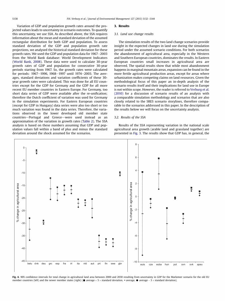
Variation of GDP and population growth rates around the pro-jected values leads to uncertainty in scenario outcomes. To quantifythis uncertainty, we use SSA. As described above, the SSA requiresinformation about themean and standard deviation of the assumedrectangular distribution for both GDP and population. To assessstandard deviation of the GDP and population growth rateprojections, we analysed the historical standard deviation for thesegrowth rates. We used the GDP and population data for 1967e2003from the World Bank database: World Development Indicators(World Bank, 2008). These data were used to calculate 30-yeargrowth rates of GDP and population for consecutive 30-yearperiods starting from 1967. So, the growth rates were calculatedfor periods: 1967e1996, 1968e1997 until 1974e2003. The aver-ages, standard deviations and variation coefficients of these 30-year growth rates were calculated. This was done for all EU coun-tries except for the GDP for Germany and the GDP for all morerecent EU member countries in Eastern Europe. For Germany, tooshort data series of GDP were available after the re-unification;therefore the Dutch coefficient of variation was used for Germanyin the simulation experiments. For Eastern European countries(except for GDP in Hungary) data series were also too short or toomuch variation was found in the data series. Therefore, the varia-tions observed in the lower developed old member statecountriesdPortugal and Greecedwere used instead as anapproximation of the variation in growth rates (Table 2). The SSAanalysis is based on these numbers assuming that GDP and pop-ulation values fall within a band of plus and minus the standarddeviation around the shock assumed for the scenarios.

-45

-40

-35

-30

-25

-20

-15

-10

-5

0

belu dnk deu grc esp fra irl ita nld aut prt fin sw

% c

hang

e in

agr

icul

tura

l are

a

Fig. 4. 90% confidence intervals for total change in agricultural land area between 2000 amember countries (left) and the newer member states (right) (- averageþ 3� standard d

3. Results

3.1. Land use change results

The simulation results of the two land change scenarios provideinsight in the expected changes in land use during the simulationperiod under the assumed scenario conditions. For both scenariosthe abandonment of agricultural area, especially in the Westernand Southern European countries, dominates the results. In EasternEuropean countries small increases in agricultural area areobserved. The spatial results show that while most abandonmenthappens inmarginal mountain areas, expansion can be found in themore fertile agricultural production areas, except for areas whereurbanization makes competing claims on land resources. Given themethodological focus of this paper an in-depth analysis of thescenario results itself and their implications for land use in Europeis not within scope. However, the reader is referred to Verburg et al.(2010) for a discussion of scenario results of an analysis witha comparable simulation methodology and scenarios that are alsoclosely related to the SRES scenario storylines, therefore compa-rable to the scenarios addressed in this paper. In the description ofthe results below we will focus on the uncertainty analysis.

3.2. Results of the SSA

Results of the SSA representing variation in the national scaleagricultural area growth (arable land and grassland together) arepresented in Fig. 3. The results show that GDP has, in general, the

e gbr-10

-8

-6

-4

-2

0

2

4

6

8

euis cze euba hun pol svn svk apeu

% c

hang

e in

agr

icul

tura

l are

a

nd 2030 resulting from uncertainty in GDP for the Marketeer scenario for the old EUeviation, ▬ average, C average� 3� standard deviation).

Fig. 5. Probability of occurrence of arable land in the year 2030 according to theMarketeer and Musketeer scenarios.

Fig. 6. Probability of occurrence of grassland in the year 2030 according to theMarketeer and Musketeer scenarios.

P.H. Verburg et al. / Journal of Environmental Management 127 (2013) S132eS144 S139

most pronounced impact on variations in land use projections.With some exceptions, the variation of land use projections ishigher for the Musketeer scenario characterized by a lower GDPgrowth than for Marketeer scenario characterized by higher GDPgrowth. The land use projections for the newer EU member coun-tries2 have higher variation since GDP and population variations arehigher for these countries than for old EU member countries.Population variation has an important impact on land in the newer

2 Newer member countries include: Poland, Czech Republic, Cyprus, Latvia,Lithuania, Slovenia, Estonia, Slovakia, Hungary, Malta, Bulgria and Romania; Oldmember countries include: Belgium, Greece, Luxembourg, Denmark, Spain,Netherlands, Germany, France, Portugal, Ireland, Italy, United Kingdom, Austria,Finland and Sweden.

EU members since population development in these countries ismore uncertain (has higher variation) than GDP; this is especiallyprominent in the Marketeer scenario where these countries facesignificant population decrease accompanied by relatively highGDP growth, which makes population a significant productionfactor in this scenario. Overall, the most obvious result from theanalysis is the high variation in sensitivity between countries.While part of this is a result of the differences in population andGDP variation, also the sensitivity of land change to these variationslargely differs between the countries.

Fig. 4 present the 90% confidence intervals for total land areachange which results from GDP uncertainty in the Marketeerscenario. The figure shows that differences in land use changes canbe very significant if GDP growth is uncertain. For example forBelgium, the decrease in agricultural area varies between 28 and 37

Fig. 7. Predicted agricultural abandonment for both scenarios for the period 2000-2030: Upper maps: percentage of agricultural area (2000 as reference) facing significantabandonment; bottom maps: percentage of agricultural area (2000 as reference) facing insignificant land abandonment.

P.H. Verburg et al. / Journal of Environmental Management 127 (2013) S132eS144S140

percent with probability of 0.9. Interestingly the higher percent-ages of variation in the newer member states result in smallerabsolute differences in agricultural area change as result of thesmaller overall levels of change. Fig. 4 also indicates that while inthe older member states themain direction is towards a decrease ofagricultural area the direction of development in the newmembersstates is somewhat mixed.

3.3. Spatial sensitivity of land allocation

The likelihoodmaps for the occurrence of arable land in 2030 forthe two scenarios are presented in Fig. 5, while Fig. 6 shows thesame for grassland. The areasmarked in blue represent areas wherearable land or grassland is likely to occur (with probability ofp > 0.95). The grey colour represents areas where arable land orgrassland is unlikely to occur (with probability of p < 0.05) and thered colour represents areas where the model produced insignifi-cant results regarding likelihood for arable or grassland(0.05 � p � 0.95), i.e. areas where the uncertainty for the occur-rence of arable land or grassland is high. For the study area as

a whole, 74% of the grassland area in 2000 is having a high likeli-hood (p > 0.95) to remain grassland in 2030. In the Musketeerscenario this is 86% of the grassland area in 2000. For arable landthese are respectively 82% and 87% for the Marketeer and Muske-teer scenario. In both scenarios and for both arable land andgrassland between 1.5% and 2.9% of the area covered by these landcover types has a high uncertainty concerning its future state(probability between 0.05 and 0.95). The remaining area (rangingfrom 12% of the arable area in the Musketeer scenario to 24% in theMarketeer scenario for grassland has a low likelihood (<0.05) toremain under the same land cover type during the 30 yearsconsidered. In both maps of Fig. 5, areas with insignificant likeli-hood for arable land tend to be located in high proximity tosignificant areas. In particular, insignificant occurrences of arableand pasture land tend to be located at the fringe of significantoccurrences; this tendency reflects areas which might becomearable land or grassland if demand for land will be relatively high.Also, areas with a high likelihood for occurrence of arable land arefound in current grassland areas and vice-versa. This is indicativefor more subtle (and uncertain) conversions in the grassland/arable

P.H. Verburg et al. / Journal of Environmental Management 127 (2013) S132eS144 S141

land mosaic in areas of intermediate suitability for arable farming.Certain areas of arable land are found in the most productiveregions while grassland has higher uncertainty both on the inter-faces with arable land and in the more marginal areas whereagricultural abandonment is an important process. A comparisonbetween the two scenarios reveals that the Marketeer scenariointroduces more areas which have insignificant probability ofarable occurrences compared to the Musketeer scenario. Areas ofconsiderable difference include the north-eastern part of Spain,Sicily, southern Romania and parts of Hungary. Similarly, also forgrassland a higher proportion of insignificant grassland area isfound in the Marketeer scenario as compared to the Musketeerscenario. Regions that exhibit considerable differences between thetwomaps include Eastern Europe and also parts of southern France.

Figs. 7 and 8 present the same model results in terms of themain processes of agricultural land change: abandonment of agri-cultural area and expansion of agricultural area over the period2000e2030. This provides a very different map as compared toFigs. 5 and 6 as possible conversions between arable land and

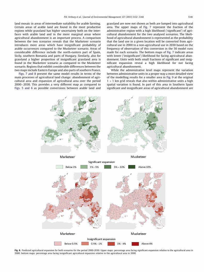
Fig. 8. Predicted agricultural expansion for both scenarios for the period 2000-2030: Upper2000; bottom maps: percentage area facing insignificant agricultural expansion relative to

grassland are now not shown as both are lumped into agriculturalarea. The upper maps of Fig. 7 represent the fraction of theadministrative region with a high likelihood (‘significant’) of agri-cultural abandonment for the two analysed scenarios. The likeli-hood of agricultural abandonment is represented as the probabilitythat the land use in a given location will be converted from agri-cultural use in 2000 to a non-agricultural use in 2030 based on thefrequency of observation of this conversion in the 50 model runsmade for each scenario. The bottom maps of Fig. 7 indicate areaswith lower (‘insignificant’) likelihood for facing agricultural aban-donment. Units with both small fractions of significant and insig-nificant expansion reveal a high likelihood for not facingagricultural abandonment.

While the administrative level maps represent the variationbetween administrative units in a proper way a more detailed viewof the modelling results for a smaller area in Fig. 9 at the original1 � 1 km grid reveals that also within administrative units a highspatial variation is found. In part of this area in Southern Spainsignificant and insignificant areas of agricultural abandonment are

maps: percentage area facing significant expansion relative to the agricultural area inthe agricultural area in 2000.

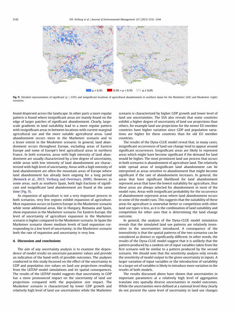
Fig. 9. Detailed representation of significant (p � 0.95) and insignificant locations of agricultural abandonment in southern Spain for the Marketeer (left) and Musketeer (right)scenarios.

P.H. Verburg et al. / Journal of Environmental Management 127 (2013) S132eS144S142

found dispersed across the landscape. In other parts a more regularpattern is found where insignificant areas are mainly found on theedge of larger patches of significant abandonment. Clearly, large-scale gradients in land suitability lead to a more regular patternwith insignificant areas in between locations with current marginalagricultural use and the more suitable agricultural areas. Landabandonment occurs more in the Marketeer scenario and toa lesser extent in the Musketeer scenario. In general, land aban-donment occurs throughout Europe, excluding areas of EasternEurope and some of Europe’s best agricultural areas in northernFrance. In both scenarios, areas with high intensity of land aban-donment are usually characterized by a low degree of uncertainty,while areas with low intensity of land abandonment are charac-terized with high level of uncertainty. Areas with a high intensity ofland abandonment are often the mountain areas of Europe whereland abandonment has already been ongoing for a long period(Renwick et al., 2013; Verburg and Overmars, 2009). However, insome areas, such as southern Spain, both high fractions of signifi-cant and insignificant land abandonment are found at the sametime (Fig. 9).

As expansion of agriculture is not a very important process inboth scenarios, very few regions exhibit expansion of agriculture.Most expansion occurs in Eastern Europe in theMusketeer scenariowhile some additional areas, like in Hungary, Romania and Spain,show expansion in the Marketeer scenario. For Eastern Europe, thelevel of uncertainty of agriculture expansion in the Marketeerscenario is higher compared to theMusketeer scenario. In Spain theMarketeer scenario shows medium levels of land expansion cor-responding to a low level of uncertainty; in the Musketeer scenarioboth the rate of expansion and uncertainty is very low.

4. Discussion and conclusions

The aim of any uncertainty analysis is to examine the depen-dence of model results on uncertain parameter values and providean indication of the band-with of possible outcomes. The analysesconducted in this study focussed on the effect of the uncertainty inGDP and population size values on land use projections resultingfrom the LEITAP model simulations and its spatial consequences.The results of the LEITAP model suggests that uncertainty in GDPhas a more pronounced impact on the uncertainty of land useprojections compared with the population size impact. TheMusketeer scenario is characterized by lower GDP growth andrelatively high level of land use uncertainties while the Marketeer

scenario is characterized by higher GDP growth and lower level ofland use uncertainties. The SSA also reveals that some countriesexhibit a higher degree of uncertainty of land use projections thanothers, for example land use projections for the newer EU membercountries have higher variation since GDP and population varia-tions are higher for these countries than for old EU membercountries.

The results of the Dyna-CLUE model reveal that, in many cases,insignificant occurrences of land use change tend to appear aroundsignificant occurrences. Insignificant areas are likely to representareas which might have become significant if the demand for landwould be higher. The most prominent land use process that occursin both scenarios is abandonment of agriculture land. The relativelywide spread areas of insignificant land abandonment can beinterpreted as areas sensitive to abandonment that might becomesignificant if the rate of abandonment increases. In general, theareas that have significant likelihood for land abandonmentrepresent areas that have the lowest suitability for agriculture, thusthese areas are always selected for abandonment in most of themodel runs. Areas with insignificant probability for the occurrenceof abandonment represent areas where land abandonment occursin some of themodel runs. This suggests that the suitability of theseareas for agriculture is somewhat better or competition with otherland use types is less, as it is the combination of land suitability andcompetition for other uses that is determining the land changeoutcome.

In general, the analysis of the Dyna-CLUE model simulationreveals that the simulated land use patterns are relatively insen-sitive to the uncertainties introduced. A consequence of theinsensitivity is that the spatial patterns of the two scenarios can beconsidered as distinct or significantly different. In other words, theresults of the Dyna-CLUE model suggest that it is unlikely that thepattern produced by a random set of input variables taken from thefirst scenario will be similar to a pattern produced by the secondscenario. We should note that the sensitivity analysis only revealsthe sensitivity of model output to the given uncertainty in inputs. Alarger variation of input variables or the introduction of variabilityto a larger set of variables is likely to introducemore variation in theresults of both models.

The results discussed above have shown that uncertainties inimportant parameters at a relatively high level of aggregationtranslate into spatially diverse uncertainties in model outcomes.While the uncertainties were defined at a national level they clearlydo not present the same level of uncertainty in land use changes

P.H. Verburg et al. / Journal of Environmental Management 127 (2013) S132eS144 S143

within the country: some areas have high certainty to face changesin land use irrespective of the uncertainty in national-leveldemographic and economic development. At the same time loca-tions that show large areas of so-called insignificant change areareas that might face agricultural land area change depending onthe change in GDP and/or demographic characteristics. Translatinguncertainties in the main drivers of integrated assessments tospatial patterns is important as the environmental changes thatpeople may face depend on the location of change. The risk ofaggregate-scale assessments is that place-based knowledge ismarginalized and globally uniform solutions are proposed to dealwith the identified problems (Hulme, 2008, 2010). Most uncer-tainty analysis in integrated environmental assessments does notaccount for the spatial variations in uncertainty, therefore beingunable tomake place-based interpretations of themeaning of theseuncertainties (van Vuuren et al., 2008). The methods described inthis paper can be applied within all probabilistic uncertaintyassessments and would facilitate in better communicating theactual meaning of uncertainty.

An important limitation of this paper is the focus on only onesource of uncertainty in assessments of land change. Only theuncertainties as result of national-level assumption of GDP andpopulation growth are evaluated within the context of twodifferent scenarios reflecting uncertainty in overall socio-economicand political developments. Although these two inputs variablesare very important determinants of land change, there are manymore input variables that are equally uncertain. Examples of otheruncertain inputs include the values of the many variables that areused in the spatial allocation of land change, including soil, climateand infrastructural conditions. Also the data on the areas of agri-cultural land use are uncertain and large deviations are foundbetween the statistical data used in the economic model and thespatial data, based on remote sensing, used in the spatial model(Verburg et al., 2011). The uncertainties in these and other variablesaffect not only the quantity of land change but also the spatialallocation of change. This is illustrated by the two scenarios that areanalysed in this paper. Not only the location of the simulated landchange is influenced by the scenario conditions, also the magnitudeand spatial spread of the uncertainty is scenario dependent.

Other uncertainties relate to the model structure, modelsimplification andmodel parameter estimates. Classical methods ofuncertainty analysis suffer from the fact that they only addressuncertainties in model inputs and neglect to examine the modelstructure itself. This critic also applies to the analysis presented inthis paper. The presented assessment methodology uses a top-down approach in which calculated changes of land use based onthe simulation of the global economy are downscaled to spatiallyexplicit patterns of land change. The local variations in land supplyand the maximum areas available for agricultural land use arerepresented in a simplified land supply function (Van Meijl et al.,2006) and are not affected by differences in spatial allocationpatterns. Also other model assumptions, such as the assumed profitoptimization in the economic model, and the location factorsselected in the land allocation models provide sources of uncer-tainty in the model outcomes.

This paper has applied a combination of a probabilistic approachand a scenario approach. While a full probabilistic approach couldbe employed to estimate the band-width of output values such anapproach only provides insight in the compound uncertainty ratherthan in the effects of uncertainty in individual variables andassumptions. Showing how uncertainties in a selected set of vari-ables result in uncertainty in output variables under particularscenario conditions provides specific information that is importantto understand under what circumstances and which areas are moreor less likely to show land changes.

Different ways of estimating the uncertainty in model parame-ters are found across the literature. For scenario assumptions it isdifficult to adequately estimate the range of uncertainties and onlythe analysis of historic variations, asmade in this paper, can providea numerical estimate of the uncertainties. Similar to Van Vuurenet al. (2008) we have used the standard deviations of historicgrowth rates as an indicator of the uncertainty. Where Van Vuurenet al. used 5e10 year growth rates we have used 30-year growthrates that correspond to the length of the simulation period. Inrecent years, the very strong fluctuation in economic growth hasshown that thus derived uncertainties may not correctly reflectthe uncertainties of reality. Observed economic growth (ordecline) rates have proven to be far outside the band-width offoreseen uncertainties already during the first few years of thesimulation period. Alternative approaches that rely less on historictrends include the use of expert knowledge in defining the possibleband-width of uncertainty within a scenario context combinedwith more in-depth simulation of the underlying processes ofdemography and economic growth (O’Neill, 2005). Whereas thisapproach may yield credible results for demographic dimensions,the unpredictability and occurrence of tipping-points in economicdevelopment make such an approach less suited for estimatinguncertainty in GDP growth rates. Interpretations of uncertaintyanalysis have, therefore, always to be interpreted with care.Consequently numerical estimates of minimum, maximum andbest guess values used in classical uncertainty analysis are oftenerroneous or misleading. We found that the spatial distribution ofcertain and less certain areas of land change is less sensitive tomodest deviations in the assumed range of uncertainties in inputvariables. This makes themaps used in this study a propermeans ofcommunicating the results of such uncertainty analysis, while atthe same time allowing an identification of which areas are actuallyaffected by these uncertainties. Uncertainty works out differentlyacross geographic space: this paper has provided an exemplar of ananalysis that accounts for such spatial variation.

Acknowledgement

Thework presented herewas carried out as part of the EuropeanUnion funded Framework Programme 6 Specific Targeted ResearchProject FARO-EU (Foresight Analysis for Rural Regions of Europe)and the Framework Programme 7 Project VOLANTE (Visions of LandUse Transitions in Europe). The authors acknowledge theconstructive comments of two anonymous reviewers.

Appendix A. Supplementary data

Supplementary data related to this article can be found at http://dx.doi.org/10.1016/j.jenvman.2012.08.038

References

Adger, W., Dessai, S., Goulden, M., Hulme, M., Lorenzoni, I., Nelson, D., Naess, L.,Wolf, J., Wreford, A., 2009. Are there social limits to adaptation to climatechange? Climatic Change 93, 335e354.

Alcamo, J., 2008. The SAS approach: combining qualitative and quantitativeknowledge in environmental scenarios. In: Joseph, A. (Ed.), Developments inIntegrated Environmental Assessment: Environmental Futures the Practice ofEnvironmental Scenario Analysis. Elsevier.

Alcamo, J., 2009. The SAS approach: combining qualitative and quantitativeknowledge in environmental scenarios. In: Alcamo, J. (Ed.), EnvironmentalFutures: The Practice of Environmental Scenario Analysis. Elsevier,Amsterdam.

Alcamo, J., Schaldach, R., Koch, J., Kölking, C., Lapola, D., Priess, J., 2011. Evaluationof an integrated land use change model including a scenario analysis of landuse change for continental Africa. Environmental Modelling & Software 26,1017e1027.

P.H. Verburg et al. / Journal of Environmental Management 127 (2013) S132eS144S144

Arndt, C., 1996. Introduction to Systematic Sensitivity Analysis via GaussianQuadrature. GTAP Technical Paper No. 2, Center for Global Trade Analysis.Purdue University. http://www.agecon.purdue.edu/gtap/techpapr/tp-2.htm.

Banse, M., van Meijl, H., Tabeau, A., Woltjer, G., Hellmann, F., Verburg, P.H., 2011.Impact of EU biofuel policies on world agricultural production and land use.Biomass and Bioenergy 35, 2385e2390.

Brian, O., 1992. Evaluating regional changes on the basis of local expectations:a visualization dilemma. Landscape and Urban Planning 21, 257e259.

Busch, G., 2006. Future European agricultural landscapesewhat can we learn fromexisting quantitative land use scenario studies? Agriculture, Ecosystems &Environment 114, 121e140.

Carter, T.R., Jones, R.N., Lu, X., Bhadwal, S., Conde, C., Mearns, L.O., O’Neill, B.C.,Rounsevell, M.D.A., Zurek, M.R., 2007. New assessment methods and the char-acterisation of future conditions. Climate change 2007: impacts, adaptation andvulnerability. In: Parry, M.L., Canziani, O.F., Palutikof, J.P., van der Linden, P.J.,Hanson, C.E. (Eds.), Contribution of Working Group II to the Fourth AssessmentReport of the Intergovernmental Panel on Climate Change. Cambridge Univer-sity Press, Cambridge.

Castella, J.C., Verburg, P.H., 2007. Combination of process-oriented and pattern-oriented models of land-use change in a mountain area of Vietnam. Ecolog-ical Modelling 202, 410e420.

CPB, 1999. World Scan: The Core Version. Netherlands Bureau for Economic PolicyAnalysis, The Hague, The Netherlands. Available at: http://www.cpb.nl.

CPB, 2003. Four Futures of Europe. Netherlands Bureau for Economic Policy Anal-ysis, The Hague, The Netherlands. Available at: http://www.cpb.nl.

Dendoncker, N., Schmit, C., Rounsevell, M., 2008. Exploring spatial data uncer-tainties in land-use change scenarios. International Journal of GeographicalInformation Science 22, 1013e1030.

Feller, W., 1968. An Introduction to Probability Theory and Its Applications, vol. 1.Wiley.

Fritz, S., See, L., McCallum, I., Schill, C., Obersteiner, M., van der Velde, M.,Boettcher, H., Havlik, P., Achard, F., 2011. Highlighting continued uncertainty inglobal land cover maps for the user community. Environmental ResearchLetters 6, 044005.

Genz, A., Bretz, F., Miwa, X., Mi, F., Leisch, F., Scheipl, F., Hothorn, T., 2012. Multi-variate Normal and T Distributions. R package version 0.9-9992. Available at:http://CRAN.R-project.org/package¼mvtnorm.

Hertel, T.W., 1997. Global Trade Analysis: Modelling and Applications. CambridgeUniversity Press, Cambridge.

Hertel, T.W., Golub, A.A., Jones, A.D., O’Hare, M., Plevin, R.J., Kammen, D.M., 2010.Effects of US maize ethanol on global land use and greenhouse gas emissions:estimating market-mediated responses. Bioscience 60, 223e231.

Heuvelink, G.B.M., Burgers, S.L.G.E., Tiktak, A., Den Berg, F.V., 2010. Uncertainty andstochastic sensitivity analysis of the GeoPEARL pesticide leaching model. Geo-derma 155, 186e192.

Hulme, M., 2008. Geographical work at the boundaries of climate change. Trans-actions of the Institute of British Geographers 33, 5e11.

Hulme, M., 2010. Problems with making and governing global kinds of knowledge.Global Environmental Change 20, 558e564.

IPCC, 2000. Special Report on Emissions Scenarios e a Special Report of WorkingGroup III of the Intergovernmental Panel on Climate Change. CambridgeUniversity Press, Cambridge UK.

Matott, L.S., Babendreier, J.E., Purucker, S.T., 2009. Evaluating uncertainty in inte-grated environmental models: a review of concepts and tools. Water ResourcesResearch 45, W06421.

Metzger, M.J., Rounsevell, M., Heiligenberg, H.A.R.M., Perez-Soba, M., Hardiman, P.S.,2010. How personal Judgment influences scenario development: an examplefor future rural development in Europe. Ecology and Society 15, 5 [online]Available at: http://www.ecologyandsociety.org/vol15/iss2/art5/.

Moss, R.H., Edmonds, J.A., Hibbard, K.A., Manning, M.R., Rose, S.K., van Vuuren, D.P.,Carter, T.R., Emori, S., Kainuma, M., Kram, T., Meehl, G.A., Mitchell, J.F.B.,Nakicenovic, N., Riahi, K., Smith, S.J., Stouffer, R.J., Thomson, A.M., Weyant, J.P.,Wilbanks, T.J., 2010. The next generation of scenarios for climate changeresearch and assessment. Nature 463, 747e756.

Nol, L., Heuvelink, G.B.M., Veldkamp, A., de Vries, W., Kros, J., 2010. Uncertaintypropagation analysis of an N2O emission model at the plot and landscape scale.Geoderma 159, 9e23.

Nol, L., Verburg, P.H., Heuvelink, G.B.M., Molenaar, K., 2008. Effect of land coverdata on N2O inventory in fen meadows. Journal of Environmental Quality 37,1209e1219.

O’Neill, B.C., 2004. Conditional probabilistic population projections: an applicationto climate change. International Statistical Review 72, 167e184.

O’Neill, B.C., 2005. Population scenarios based on probabilistic projections: anapplication for the Millennium Ecosystem assessment. Population & Environ-ment 26, 229e254.

Overmars, K.P., Verburg, P.H., 2006. Multilevel modelling of land use from field tovillage level in the Philippines. Agricultural Systems 89, 435e456.

Pidgeon, N., Fischhoff, B., 2011. The role of social and decision sciences incommunicating uncertain climate risks. Nature Climate Change 1, 35e41.

Polasky, S., Carpenter, S.R., Folke, C., Keeler, B., 2011. Decision-making under greatuncertainty: environmental management in an era of global change. Trends inEcology & Evolution 26, 398e404.

Pontius, J., Petrova, S.H., 2010. Assessing a predictive model of land change usinguncertain data. Environmental Modelling & Software 25, 299e309.

Pontius, R., Boersma, W., Castella, J.-C., Clarke, K., de Nijs, T., Dietzel, C., Duan, Z.,Fotsing, E., Goldstein, N., Kok, K., Koomen, E., Lippitt, C., McConnell, W., MohdSood, A., Pijanowski, B., Pithadia, S., Sweeney, S., Trung, T., Veldkamp, A.,Verburg, P., 2008. Comparing the input, output, and validation maps for severalmodels of land change. Annals of Regional Science 42, 11e37.

Pontius, R.G., Huffaker, D., Denman, K., 2004. Useful techniques of validation forspatially explicit land-change models. Ecological Modelling 179, 445e461.

Priess, J.A., Schaldach, R., 2008. Integrated models of the land system: a review ofmodelling approaches on the regional to global scale. Living Reviews in Land-scape Research vol. 2.

Refsgaard, J.C., van der Sluijs, J.P., Højberg, A.L., Vanrolleghem, P.A., 2007. Uncer-tainty in the environmental modelling process e a framework and guidance.Environmental Modelling & Software 22, 1543e1556.

Renwick, A., Jansson, T., Verburg, P.H., Revoredo-Giha, C., Britz, W., Gocht, A.,McCracken, D., 2013. Policy reform and agricultural land abandonment in theEU. Land Use Policy 30, 446e457.

Rounsevell, M.D.A., Reginster, I., Araújo, M.B., Carter, T.R., Dendoncker, N., Ewert, F.,House, J.I., Kankaanpää, S., Leemans, R., Metzger, M.J., Schmit, C., Smith, P.,Tuck, G., 2006. A coherent set of future land use change scenarios for Europe.Agriculture, Ecosystems & Environment 114, 57e68.

Schaldach, R., Alcamo, J., Koch, J., Kölking, C., Lapola, D.M., Schnngel, J., Priess, J.A.,2011. An integrated approach to modelling land-use change on continental andglobal scales. Environmental Modelling & Software 26, 1041e1051.

Tebaldi, C., Smith, R.L., Nychka, D., Mearns, L.O., 2005. Quantifying uncertainty inprojections of regional climate change: a Bayesian approach to the analysis ofMultimodel Ensembles. Journal of Climate 18, 1524e1540.

Turner, B.L., Lambin, E.F., Reenberg, A., 2007. The emergence of land change sciencefor global environmental change and sustainability. Proceedings of the NationalAcademy of Sciences of the United States of America 104, 20666e20671.

van Asselt, M., Rotmans, J., 1996. Uncertainty in perspective. Global EnvironmentalChange 6, 121e157.

Van Meijl, H., van Rheenen, T., Tabeau, A., Eickhout, B., 2006. The impact of differentpolicy environments on agricultural land use in Europe. Agriculture, Ecosys-tems & Environment 114, 21e38.

van Vuuren, D.P., de Vries, B., Beusen, A., Heuberger, P.S.C., 2008. Conditionalprobabilistic estimates of 21st century greenhouse gas emissions based onthe storylines of the IPCC-SRES scenarios. Global Environmental Change 18,635e654.

Verburg, P.H., Schot, P.P., Dijst, M.J., Veldkamp, A., 2004. Land use change modelling:current practice and research priorities. GeoJournal 61, 309e324.

Verburg, P.H., van Berkel, D.B., van Doorn, A.M., van Eupen, M., van denHeiligenberg, H.A.R.M., 2010. Trajectories of land use change in Europe:a model-based exploration of rural futures. Landscape Ecology 25, 217e232.

Verburg, P.H., Eickhout, B., van Meijl, H., 2008. A multi-scale, multi-model approachfor analyzing the future dynamics of European land use. Annals of RegionalScience 42, 57e77.

Verburg, P.H., Neumann, K., Nol, L., 2011. Challenges in using land use and landcover data for global change studies. Global Change Biology 17, 974e989.

Verburg, P.H., Overmars, K., 2009. Combining top-down and bottom-up dynamics inland use modeling: exploring the future of abandoned farmlands in Europewith the Dyna-CLUE model. Landscape Ecology 24, 1167e1181.

Verburg, P.H., Rounsevell, M.D.A., Veldkamp, A., 2006. Scenario-based studies offuture land use in Europe. Agriculture, Ecosystems & Environment 114, 1e6.

Walker, R., 2003. Evaluating the performance of spatially explicit models. Photo-grammetric Engineering & Remote Sensing 69, 1271e1278.

Westhoek, H.J., van den Berg, M., Bakkes, J.A., 2006. Scenario development toexplore the future of Europe’s rural areas. Agriculture, Ecosystems & Environ-ment 114, 7e20.

World Bank, 2008. World Development Indicators 2008. Word Bank, Washington,USA.