U.S. Fish and Wildlife Service Office of Subsistence Management

Fisheries Resource Monitoring Program

Assessing Methods to Index Inseason Salmon Abundance in the Lower Copper River, 2003 Annual Report

Annual Report No. FIS01-021

March 2004

U.S. Fish and Wildlife Service Office of Subsistence Management

Fisheries Resource Monitoring Program

Assessing Methods to Index Inseason Salmon Abundance in the Lower Copper River, 2003 Annual Report

Annual Report No. FIS01-021

Don Degan, Anna Maria Mueller

Aquacoustics, Inc. P.O. Box 1473

Sterling, AK 99672-1473

Jason J. Smith

LGL Alaska Research Associates, Inc. 1101 E 76th Ave., Suite B Anchorage, AK 99516

Steve Moffitt, Nancy Gove

Alaska Department of Fish and Game P.O. Box 669

Cordova, Alaska 99574

March 2004

Annual Report Summary Page

Title: Assessing Methods to Index Inseason Salmon Abundance in the Lower Copper River, 2003 Annual Report Study Number: FIS01-021 Investigators/Affiliations: Bruce Cain/Native Village of Eyak; Michael Link/LGL Alaska Research Associates, Inc.; Steve Moffitt/Alaska Department of Fish and Game, Commercial Fisheries Division; Don Degan/Aquacoustics, Inc. Management Regions: Cook Inlet/Gulf of Alaska Information types: Stock Status Trends, Fisheries Monitoring Issues Addressed: Improve inseason escapement indices of salmon in the lower Copper River, downstream of the Miles Lake sonar site. Study Cost: $509,975 (three-year total) Study Duration: March 2001 – February 2004 Key Words: Copper River, inseason management, sockeye salmon, Oncorhynchus nerka, Chinook salmon, Oncorhynchus tshawytscha, subsistence fishery, drift gillnet, acoustics, Native Village of Eyak. Citation: Degan, D. J., A. M. Mueller, J. J. Smith, S. Moffitt and N. Gove. 2004. Assessing methods to index inseason salmon abundance in the lower Copper River, 2003 Annual Report. USFWS Office of Subsistence Management, Fisheries Resource Monitoring Program, Annual Report No. FIS01-021, Anchorage, Alaska.

TABLE OF CONTENTS

LIST OF FIGURES ........................................................................................................................ ii

LIST OF TABLES......................................................................................................................... iv

EXECUTIVE SUMMARY ........................................................................................................... vi

INTRODUCTION .......................................................................................................................... 1

Study Area .................................................................................................................................. 2 Objectives ................................................................................................................................... 2

METHODS ..................................................................................................................................... 3

Acoustics..................................................................................................................................... 4 Site Selection .......................................................................................................................... 4 Equipment Setup and Operation ............................................................................................. 5 Data Analysis .......................................................................................................................... 6

Drift Gillnetting .......................................................................................................................... 7 Site Selection .......................................................................................................................... 8 Setup and Operation................................................................................................................ 8 Test Fishing Index................................................................................................................... 8

Forecasting Miles Lake Sonar Counts Using Flag Point Channel Indices ................................. 9 RESULTS ..................................................................................................................................... 10

Acoustics................................................................................................................................... 11 Equipment Setup and Operation ........................................................................................... 11 Target Strength Filter for Salmon and Fish Behavior........................................................... 11

Drift Gillnetting ........................................................................................................................ 13 Acoustic and Drift Gillnetting Indices at Flag Point Channel .................................................. 13 Forecasting Miles Lake Sonar Counts Using Flag Point Channel Indices ............................... 14

DISCUSSION............................................................................................................................... 15

Acoustics................................................................................................................................... 15 Flag Point Channel Indices as a Management Tool.................................................................. 16 Acoustics and Drift Gillnetting: Strengths and Weaknesses ................................................... 17

CONCLUSIONS........................................................................................................................... 18

RECOMMENDATIONS.............................................................................................................. 18

ACKNOWLEDGMENTS ............................................................................................................ 19

LITERATURE CITED ................................................................................................................. 20

FIGURES...................................................................................................................................... 21

TABLES ....................................................................................................................................... 39

APPENDICES .............................................................................................................................. 43

i

LIST OF FIGURES Figure 1. Map of the lower Copper River in Alaska showing the location of Flag Point

Channel and the Miles Lake sonar site, 2003.

Figure 2. Bathymetry of the acoustic sampling site used in 2002 and 2003 which was located at Flag Point Channel 400 m downstream of Bridge 331 on the Copper River Highway. Figure 3. Aerial photograph of the Copper River Highway (Mile 27) and Flag Point Channel.

Figure 4. Design of the transducer mount showing the location of the (1) transducer, (2) attitude sensor, (3) float switch (4) setscrews for adjusting the vertical position and (5) tilt angle of the transducer.

Figure 5. Platform for the streamside equipment which consisted of (1) a fish tote that housed the DTX echosounder, wireless Ethernet bridge, fuse bank, battery bank, charger and charge controller, (2) a wireless Ethernet antenna, (3) a wind generator and (4) the solar panels. Figure 6. Location of the travel trailer which served as the data retrieval and processing station and accommodation for the technicians.

Figure 7. Frequency distribution of the average target strength of fish tracked at Flag Point

Channel on the Copper River, 2003. Figure 8. Daily average and daily maximum of the average target strength of fish tracked at

Flag Point Channel on the Copper River, 2003. Figure 9. Distribution of x-speed and target strength for all tracked targets, 2003. Figure 10. Profile of the river bottom and vertical distribution of fish over range at the

acoustic sampling site at Flag Point Channel, 2003. Figure 11. Direction of movement and range of salmon-sized targets that were tracked at

Flag Point Channel on the Copper River, 2003. Figure 12. Daily acoustic counts for salmon that were generated from different counting

methods and sampling schemes at Flag Point Channel, 2003. Figure 13. Linear regression of full and subsampled tracked counts for salmon at Flag Point

Channel on the Copper River, 2003.

ii

LIST OF FIGURES (continued) Figure 14. Daily acoustic (tracked, fully sampled data) and drift gillnetting indices for

salmon at Flag Point Channel, sonar counts from Miles Lake and the starting dates of commercial fishing openings in the Copper River District, 2003.

Figure 15. Catch efficiency of acoustics and drift gillnetting, as measured by the ratio of the

Flag Point Channel index to the Miles Lake sonar count lagged by 1 day (index per 1000 fish counted; 3-day moving average), and the Copper River stage height at Flag Point Channel, 2003.

Figure 16. Mean percentage forecast error (MPE) for drift gillnetting and acoustics in the

lower Copper River at Flag Point Channel, 2001-2003. Figure 17. Mean absolute percentage forecast error (MAPE) for drift gillnetting and

acoustics in the lower Copper River at Flag Point Channel, 2001-2003.

iii

LIST OF TABLES Table 1. Sampling effort and range of the acoustic equipment that was operated at Flag

Point Channel on the Copper River, 2003. Table 2. Daily acoustic counts for salmon that were generated from different counting

methods and sampling schemes at Flag Point Channel, 2003. Table 3. Effort, catch and the test fishing index for the drift gillnetting operation at Flag Point Channel on the Copper River, 2003.

iv

LIST OF APPENDICES Appendix A – Acoustic Counting Guidelines and Calibration Parameters Figure A-1. An EchoView® target-strength echogram showing track examples with guidelines

for visually counting salmon-sized fish. Figure A-2. An EchoView® angle echogram showing track examples with guidelines distinguishing a disrupted track caused by a single fish from tracks caused by multiple fish. Table A-1. Single target-detection algorithm and calibration parameters for the acoustic

equipment used at Flag Point Channel on the Copper River, 2003. Appendix B – Copper River Water Levels Figure B-1. Stage height of the Copper River at Flag Point Channel and the Million Dollar

Bridge, 2003. Table B-1. Stage height of the Copper River at Flag Point Channel and the Million Dollar

Bridge, 2003. Appendix C – 2002 Miles Lake Sonar counts Table C-1. Daily salmon counts and escapement objectives at the Miles Lake sonar, 2003.

v

EXECUTIVE SUMMARY The purpose of this three-year project (2001-2003) was to develop and assess methods of monitoring salmon escapement in the lower Copper River. The ultimate goal was to develop an annual monitoring program that could provide fishery managers with more timely indices of salmon escapement than those currently available from the Miles Lake sonar site (river km 52). A multi-faceted research design was developed to (1) significantly shorten the development time of a lower river test fishery; (2) study fish migratory behavior; and (3) compare the utility of acoustics and drift gillnets as test fishing tools. This report presents results from the third year of operation.

Almost continuous acoustic sampling was conducted at Flag Point Channel on the Copper River from 8 May to 6 June 2003. A combination of counting methods (directly from echograms and tracked with acoustic software) and sampling schemes (fully sampled and subsampled hourly data) were used to generate counts from the acoustic data. A total of 1,902 salmon were counted with a peak of 324 fish on 2 June. There was considerable uncertainty in the 2003 acoustic counts because the frequency distribution of target strengths did not show a clear mode for separating eulachon Thaleichthys pacificus from salmon-sized targets. Drift gillnetting was conducted at Flag Point Channel from 6 May to 6 June 2003. A total of 201 sockeye salmon Oncorhynchus nerka were captured during 3,077 min of fishing. Daily test fishing indices (fish per 100 fathom hours) for sockeye salmon peaked at 179 on 29 May, and the season cumulative index was 1,109. Due to anomalously low water levels, acoustic and drift gillnetting methods were unable to effectively index the abundance of early-run salmon in the lower Copper River in 2003 or to track the general trends in abundance observed at the Miles Lake sonar site. Similar to previous years, estimated travel time between Flag Point Channel and the Miles Lake sonar ranged from 1-3 d, with the best model fits produced by estimates of 2-3 d lags. As in 2002, fish appeared to take 1-2 d to travel the 16-km distance between the Copper River ocean fishing district and the Flag Point Channel sample site. Based on the relative strengths and weaknesses of each sampling technique, project investigators recommend acoustics for continued use to index the abundance of salmon in the lower Copper River in 2004.

vi

INTRODUCTION

The purpose of this three-year project (2001-2003) was to develop and assess methods of monitoring salmon escapement in the lower Copper River. The ultimate goal was to develop an annual monitoring program that could provide fishery managers with more timely indices of salmon escapement than those currently available from the Miles Lake sonar site (river km 52). The Copper River subsistence and commercial salmon fisheries are of great value to both native and non-native participants. In 2001, the Alaska Department of Fish and Game (ADF&G) gave permits to more than 10,000 people to fish the Copper River subsistence fisheries with an estimated total harvest of Chinook Oncorhynchus tshawytscha, sockeye O. nerka and coho O. kisutch salmon of 226,420 (Gray et al. 2002). In the Copper River District, the ex-vessel value of commercial, common-property, salmon landings exceeded $14 million in 2002. Recent (1991-2000) average commercial harvests of sockeye and Chinook salmon have been 1,521,641 and 48,640, respectively (Gray et al. 2002). From 1990 through 1999, sport harvests for sockeye and Chinook salmon have averaged 12,000 fish (Taube and Sarafin 2001). Most of the Copper River subsistence harvest is taken in the upper river and its tributaries, 150 km or more upstream of the ocean commercial fishery. Therefore, migrating fish are exposed to commercial fishing activity from two to four weeks (depending in part on river discharge) before they arrive in the major subsistence fishing areas (Merritt and Roberson 1986). The lack of early run assessment information can make it difficult for managers to meet escapement goals while providing a sufficient number of fish for subsistence and commercial harvesters. The commercial salmon fishery also covers a large area (~1,200 km2), and the rate at which salmon migrate through this area during the early part of the season varies among years. For example, if fish move quickly from the Copper River District into the river, the commercial fishery may forego harvests at a time when the landed value of the fish is 100-200% greater than it is later in the season. On the other hand, if fish mill in the Copper River District while waiting for appropriate conditions to move into the river, they may be subject to excess commercial fishing pressure. Much effort has been expended over the last 40 years to develop a timely method of estimating salmon escapement for the Copper River. In 1978, a Bendix sonar system was placed 52 km (33 miles) upriver of the Copper River District, just below the outlet of Miles Lake where the river is confined to a single channel. This sonar system has provided a daily index of salmon abundance since 1978. However, data gathered by ADF&G suggested that it could take anywhere from three to nine days for sockeye salmon to travel from the Copper River District to the Miles Lake sonar site (Roberson et al. 1980; Schaller 1984). As a result, fishery managers faced difficult decisions early in the season because in addition to variable travel times, the timing of river entry is highly variable among years (Schaller 1984). In late June 1984, ADF&G assessed the utility of using a Bendix sonar counter about half way between Miles Lake and the commercial fishery (Steve Moffitt, ADF&G, Commercial Fisheries Division, personal communication). The counts were generally 10-100 fish per day, but the work was hindered by high water levels and debris. A more extensive survey planned for 1985 was not funded. In 2003, ADF&G began testing a dual-frequency identification sonar (DIDSON) on a new artificial

1

substrate at the Miles Lake site. It is anticipated that the DIDSON will replace the Bendix sonar by 2006. The Miles Lake sonar site provides relatively reliable daily and annual indices of salmon abundance and will probably do so well into the future. However, the early commercial fishing periods could be managed with greater confidence if abundance estimates were available earlier in the season. In 2000, under renewed pressure from commercial and subsistence users, ADF&G initiated a study to assess the feasibility of an early-season, test-netting program in the Copper River Delta (Moffitt et al. 2000). Drift dip netting and drift gillnetting were investigated as possible means to index salmon returns in the lower part of the river; however, ADF&G found that dip nets would not catch enough fish to provide a reliable index without a significant increase in fishing effort. With many Tribal members heavily reliant upon subsistence and commercial fisheries, the Native Village of Eyak (NVE) understood the value and importance of improving early season indices of salmon abundance in the Copper River. In 2000, NVE worked with LGL Alaska Research Associates, Inc. (LGL) and ADF&G to design a multi-faceted study design to (1) significantly shorten the development time of a lower river test fishery; (2) study fish migratory behavior; and (3) compare the utility of acoustics and drift gillnets as test fishing tools.

Study Area

The Copper River flows through the Chugach Mountains of Alaska and drains into the northern limits of the Gulf of Alaska, east of Prince William Sound (Fig. 1). Including its tributaries, the Copper River stretches more than 466 km and has created a 70-km wide delta of primarily glacial silt (Brabets 1997). The average annual discharge of the Copper River is 1,625 m3/s, the second largest in Alaska. Despite carrying a very high sediment load, the Copper River is the largest salmon-producing river in Central Alaska (Merritt and Roberson 1986) and supports abundant populations of sockeye and Chinook salmon.

Objectives

The purpose of this project was to generate a timely inseason index of salmon abundance that could be used to help manage the commercial fishery and ensure an adequate number of fish escape upriver for spawning requirements and subsistence users. Overall goals for this three-year project were to:

1) Determine the migratory behavior and stream channel use of early-run sockeye salmon in the lower Copper River to gauge the sampling effort that is required to index inseason salmon abundance;

2) Assess the efficacy of sonar and drift gillnetting to provide a daily inseason index of early-run salmon abundance in the lower Copper River; and

3) Assess the feasibility of operating sonar and drift gillnetting test fisheries.

2

In the first two years of this project, both acoustics and drift gillnetting were used at Flag Point Channel on the Copper River near Bridge 331 on the Copper River Highway. Test fishing indices from both sampling gears were quite similar and tracked well with counts at the Miles Lake sonar site. The travel time of sockeye salmon from Flag Point Channel to the Miles Lake sonar ranged from one to two days in 2001 and one to three days in 2002. Fish also appeared to move quickly (1 to 2 d) from the Copper River District to Flag Point Channel (Link et al. 2001; Lambert et al. 2003).

In 2001 and 2002, acoustic sampling was also performed at the Mile-37 Channel, located on the west bank of the river near Bridge 342 on the Copper River Highway. It was thought that acoustic data collected at the Mile-37 Channel could help explain trends in fish passage at Flag Point Channel as well as provide an alternative site for indexing salmon abundance in the lower Copper River. However, the short travel time of salmon from Flag Point Channel to the Miles Lake sonar reduced the value of Mile-37 as a potential index site. The benefits of sampling at the Mile-37 Channel appeared too small to justify the added cost to the project so it was discontinued after the 2002 season.

Specific objectives for the 2003 lower river test fishery (LRTF) project were to: 1) Sample with acoustics and drift gillnets at Flag Point Channel and provide daily

inseason counts to ADF&G fishery managers; 2) Train NVE technicians to operate acoustic equipment, count from echograms and

manage sonar data in an effort to reduce the role of consultants in the day-to-day operations of the project;

3) Adapt the acoustics setup for remote operation to ensure a smooth transition, if necessary, to a new sampling site in the lower Copper River;

4) Assess the among-year variability in travel times and fish behavior; and 5) Compare the relative strengths and weaknesses of acoustics and drift gillnetting and

identify the most cost-effective technique (i.e., accuracy vs. cost) for indexing salmon abundance in the lower Copper River.

METHODS

Daily sampling of a consistent portion of the total fish run is required for successful and economical indexing of salmon abundance. The portion of a run sampled by a “test fishery” (e.g., 0.01 or 1%) for a given level of effort (e.g., 30 m of gillnet for 30 min or 15 min of acoustic sampling) is referred to as the catchability coefficient of the test fishery. The catchability coefficient is usually determined by comparing the daily (or cumulative) test fishing indices with an independent measure of the total daily (or cumulative) fish passage. The catchability coefficient of a test fishery must be consistent both within and among years for the test fishery to be useful. Therefore, it is best to sample at times and locations where the catchability coefficient is expected to be consistent among days and among years.

3

River stage height and weather information were recorded on most sampling days. Stage height was measured at a U.S. Geological Survey (USGS) gauge mounted on Bridge 331 and provided a relative measure of river elevation (the elevation of the bridge above sea level was not known). Stage height data was also obtained from a USGS gauge mounted on Million Dollar Bridge located at the outlet of Miles Lake. Weather information collected each day included cloud cover, precipitation, wind velocity (km/h) and wind direction.

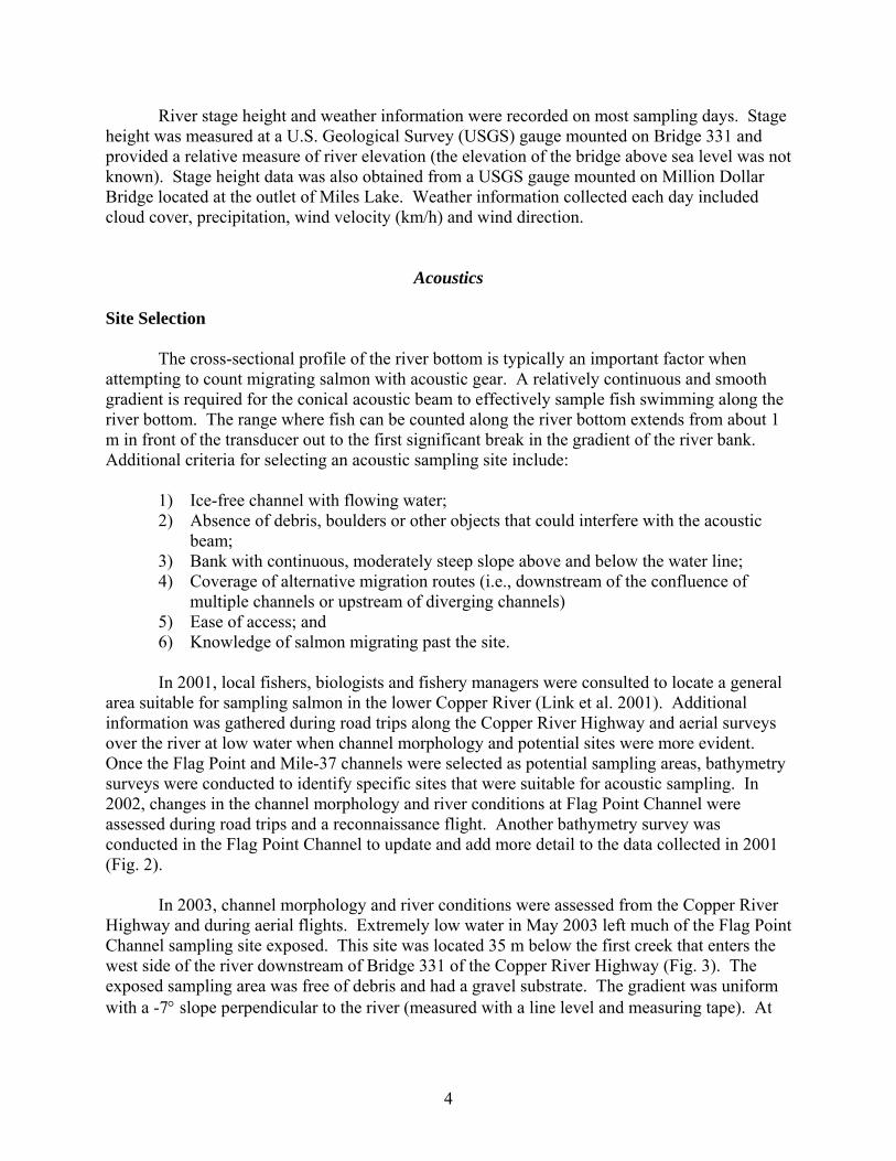
Acoustics Site Selection

The cross-sectional profile of the river bottom is typically an important factor when attempting to count migrating salmon with acoustic gear. A relatively continuous and smooth gradient is required for the conical acoustic beam to effectively sample fish swimming along the river bottom. The range where fish can be counted along the river bottom extends from about 1 m in front of the transducer out to the first significant break in the gradient of the river bank. Additional criteria for selecting an acoustic sampling site include:

1) Ice-free channel with flowing water; 2) Absence of debris, boulders or other objects that could interfere with the acoustic

beam; 3) Bank with continuous, moderately steep slope above and below the water line; 4) Coverage of alternative migration routes (i.e., downstream of the confluence of

multiple channels or upstream of diverging channels) 5) Ease of access; and 6) Knowledge of salmon migrating past the site.

In 2001, local fishers, biologists and fishery managers were consulted to locate a general

area suitable for sampling salmon in the lower Copper River (Link et al. 2001). Additional information was gathered during road trips along the Copper River Highway and aerial surveys over the river at low water when channel morphology and potential sites were more evident. Once the Flag Point and Mile-37 channels were selected as potential sampling areas, bathymetry surveys were conducted to identify specific sites that were suitable for acoustic sampling. In 2002, changes in the channel morphology and river conditions at Flag Point Channel were assessed during road trips and a reconnaissance flight. Another bathymetry survey was conducted in the Flag Point Channel to update and add more detail to the data collected in 2001 (Fig. 2).

In 2003, channel morphology and river conditions were assessed from the Copper River

Highway and during aerial flights. Extremely low water in May 2003 left much of the Flag Point Channel sampling site exposed. This site was located 35 m below the first creek that enters the west side of the river downstream of Bridge 331 of the Copper River Highway (Fig. 3). The exposed sampling area was free of debris and had a gravel substrate. The gradient was uniform with a -7° slope perpendicular to the river (measured with a line level and measuring tape). At

4

higher water levels, the site was well suited for acoustic sampling, so no bathymetry survey was conducted in 2003. Equipment Setup and Operation

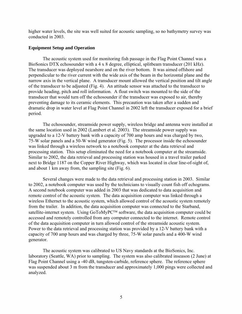
The acoustic system used for monitoring fish passage in the Flag Point Channel was a BioSonics DTX echosounder with a 4 x 8 degree, elliptical, splitbeam transducer (201 kHz). The transducer was deployed nearshore and on the river bottom. It was aimed offshore and perpendicular to the river current with the wide axis of the beam in the horizontal plane and the narrow axis in the vertical plane. A transducer mount allowed the vertical position and tilt angle of the transducer to be adjusted (Fig. 4). An attitude sensor was attached to the transducer to provide heading, pitch and roll information. A float switch was mounted to the side of the transducer that would turn off the echosounder if the transducer was exposed to air, thereby preventing damage to its ceramic elements. This precaution was taken after a sudden and dramatic drop in water level at Flag Point Channel in 2002 left the transducer exposed for a brief period.

The echosounder, streamside power supply, wireless bridge and antenna were installed at the same location used in 2002 (Lambert et al. 2003). The streamside power supply was upgraded to a 12-V battery bank with a capacity of 700 amp hours and was charged by two, 75-W solar panels and a 50-W wind generator (Fig. 5). The processor inside the echosounder was linked through a wireless network to a notebook computer at the data retrieval and processing station. This setup eliminated the need for a notebook computer at the streamside. Similar to 2002, the data retrieval and processing station was housed in a travel trailer parked next to Bridge 1187 on the Copper River Highway, which was located in clear line-of-sight of, and about 1 km away from, the sampling site (Fig. 6).

Several changes were made to the data retrieval and processing station in 2003. Similar to 2002, a notebook computer was used by the technicians to visually count fish off echograms. A second notebook computer was added in 2003 that was dedicated to data acquisition and remote control of the acoustic system. The data acquisition computer was linked through a wireless Ethernet to the acoustic system, which allowed control of the acoustic system remotely from the trailer. In addition, the data acquisition computer was connected to the Starband, satellite-internet system. Using GoToMyPC™ software, the data acquisition computer could be accessed and remotely controlled from any computer connected to the internet. Remote control of the data acquisition computer in turn allowed control of the streamside acoustic system. Power to the data retrieval and processing station was provided by a 12-V battery bank with a capacity of 700 amp hours and was charged by three, 75-W solar panels and a 400-W wind generator.

The acoustic system was calibrated to US Navy standards at the BioSonics, Inc. laboratory (Seattle, WA) prior to sampling. The system was also calibrated inseason (2 June) at Flag Point Channel using a -40 dB, tungsten-carbide, reference sphere. The reference sphere was suspended about 3 m from the transducer and approximately 1,000 pings were collected and analyzed.

5

When sampling fish, the transducer was aimed along the river bottom. The aim of the transducer was verified using a plastic sphere (10-cm dia) with target strength similar to an adult salmon. The sphere was lowered in front of the transducer using a fishing rod, raised 15 cm off the river bottom and then moved in- and offshore as much as water depth and current allowed. The aim of the transducer was confirmed when the target echoes were clearly visible and strong enough to qualify as salmon over at least every 0.5 m of the range. Fish were sampled with a ping rate of 15 pings per second, a pulse length of 0.2 milliseconds and a data collection threshold of -55 dB.

A weir made from rebar and construction fencing was used to keep fish from passing too close to the transducer where the acoustic beam is not coherently formed or too small to efficiently detect fish. Technicians regularly removed debris from the weir and the transducer mount and wiped algae growth off the transducer face.

Data Analysis

Three counting methods (visual, tracked and tracked net upstream) and two sampling schemes (full and subsampled) were used to generate counts from acoustic data (see table on p. 7 for descriptions). Visual counts were based on echo traces seen on echograms and did not account for the direction of target movement (i.e., upstream or downstream). Echograms were displayed in EchoView 3.00 software. Target strength (TS) echograms and predetermined guidelines (Fig. A-1) were used to separate salmon from smaller fish such as eulachon Thaleichthys pacificus. Target-strength echograms were color-coded by target strength where warmer colors indicated stronger targets. With the color display set to a minimum of -55 dB and range of 40 dB, tracks had to include echoes in turquoise or warmer colors to be counted as salmon.

Technicians were shown how to use angle echograms to decide whether tracks were caused by a single fish (disrupted track) or multiple fish (Fig. A-2). The colors in angle echograms indicate the upstream or downstream angle at which the targets are seen. Targets in cool colors are seen on the downstream side of the transducer, while targets in warm colors are seen on the upstream side of the transducer. A fish that is moving upstream will typically be seen as a track that starts in dark blue, changes to light blue and turquoise as it approaches the center line of the beam, and turns green, yellow and eventually red as it leaves the beam on the upstream side of the transducer. The track of a fish that is moving downstream will change colors in reverse order (i.e., from red to yellow, green, turquoise, light blue and then dark blue). To stay consistent with 2002 inseason visual counts, the direction of target movement was ignored despite the fact this color scheme allowed the distinction between upstream and downstream moving fish.

Most visual counts were based on reviewing the first 15-min file of each hour sampled.

If the first file of the hour was less than 15-min long then the second or third file was used instead. Files were 20-min long at the beginning of the season (8-14 May), and intermittently throughout the sampling period some files were 30-min long. Hourly counts were expanded in proportion to the time counted (i.e., 15-min counts were multiplied by 4, 20-min counts by 3, 30-min counts by 2). Daily visual counts were expanded by the proportion of missing hours. This

6

expansion method was used to be consistent with all other counts, including full counts, but differs slightly from the method used inseason. Inseason visual counts were expanded for missing hours by taking the average of the last good hour before the data gap and the first good hour after the gap. Category Description

Counting MethodVisual Fish echo traces were counted directly from the echogramTracked

Tracked netupstream

Sampling SchemeFull Based on sampling complete hoursSubsampled Based on sampling 15 minutes of each hour

Fish echo traces were counted with acoustic, target-tracking software that ignored the direction the target movementFish echo traces were counted with acoustic, target-tracking software that subtracted the number of downstream-moving targets from the number of upstream-moving targets

Tracked counts were generated with EchoView 3.00 software using an alpha-beta track-detection algorithm (Table A-1). Tracked files were reviewed and edited manually by removing obvious non-salmon targets (e.g., rocks and eulachon), merging split tracks and splitting merged tracks. The size distribution of all tracked targets was examined to determine a suitable threshold for separating eulachon, some of which were included in the tracking output, from salmon. Only tracks with average target strengths greater than the threshold value were included in the counts. Daily tracked counts were expanded by the proportion of time not sampled on a given day. Similar to visual counts, tracked counts did not account for the direction of target movement.

Tracked net upstream counts were generated from tracked counts (fully sampled hourly data) by subtracting the number of downstream-moving targets from the number of upstream-moving targets. The direction of target movement was determined from the slope of a linear regression of x-position (i.e., upstream-downstream) and time. Tracks with a positive slope were classified as moving upstream, while tracks with a negative slope were classified as moving downstream.

Drift Gillnetting

As in 2001 and 2002, ADF&G used drift gillnets to index the abundance of sockeye salmon in the lower Copper River in 2003. Most of the net sampling occurred in Flag Point Channel below Bridge 331 on the Copper River Highway and above the fork of the Pete Dahl Slough (Fig. 1).

7

Site Selection Flag Point Channel was selected for drift gillnetting because it was a constriction point where most of the west side of the Copper River was contained within a single channel. The channel reach starts approximately 21.6 km above the Copper River District markers at Castle Island Channel, and there is no apparent tidal influence. Flag Point Channel was the preferred site for drift gillnetting because:

1) It was road accessible most years by early to mid-May; 2) It had a good beach for launching boats; 3) It could be fished on a daily basis without a field camp; and 4) The water velocity was significantly slower than in other channels.

Setup and Operation

The drift gillnets used in 2003 were either 18.3 m (10 fathoms) or 36.6 m (20 fathoms) long and 20 meshes deep with a 13.7 cm (5 3/8 in), stretched-mesh web. In 2001 and 2002 only 18.3 m long drift gillnets were used. Three different stations were sampled on a regular basis by the ADF&G crew in 2003. Most drift gillnet sets were made perpendicular to shore and as close to the bank as possible because most sockeye salmon travel upriver near the bank (Burgner 1991). Tension was placed on the net as required to keep it from bunching up in the current. The starting and stopping points for each drift were marked with surveyors flagging on bank vegetation. Due to the numerous snags embedded in the river bottom along the west bank, each set was limited to approximately 2 min fishing time in 2001 and 2002. In 2003 sets of much longer duration were made prior to 28 May because of the low river levels and slow velocity currents.

For each set, the following data were recorded: set location, distance offshore at the start and end of a drift, time the net started out, time the net was completely out, time the net started in, time the net was completely in and number of fish captured by species. All captured fish were marked by clipping the adipose fin and then released if in good condition. Unreleased fish were sampled for length, weight, sex and age. Test Fishing Index The daily test fishing index for drift gillnetting at Flag Point Channel was calculated as in Gray (2000). Mean fishing time (M, min) was computed for each set:

,2

SI)-(FI + SO)-(FO + FO - SI= MT (1)

where SO was the time the gillnet first entered water, FO the time the gillnet was fully deployed, SI the time gillnet retrieval began, and FI the time gillnet retrieval was completed. Catch-per-unit-effort (CPUE, Cj), or the number of sockeye salmon caught per 100 fathom hours, was computed for set j by the following equation:

8

,MTxG

N6,000 = C j (2)

where N was the number of sockeye salmon caught and G the gillnet length in fathoms. The daily test fishing index at Flag Point Channel, Ii, for day i was computed as the mean of the CPUE values from the number of sets (Si) made on day i:

.

i

C = I

s

j

s

1=ji

∑ (3)

Forecasting Miles Lake Sonar Counts Using Flag Point Channel Indices

The real need on the Copper River is a tool for forecasting inseason escapement levels

between the Copper River District commercial fishery and the Miles Lake sonar site, particularly at the beginning of the fishing season. For this study, the ability of acoustic (subsampled tracked counts) and drift gillnetting data collected at Flag Point Channel to forecast Miles Lake sonar counts was evaluated. Miles Lake sonar counts were lagged to account for the travel time of sockeye salmon from the test fishing sites at Flag Point Channel to the Miles Lake sonar site. Maximum likelihood estimation (MLE) and regression analysis were used to compare both sampling gears for lags of one, two and three days.

To emulate inseason forecasting, only data collected up to the day of the forecast were

used, and the first forecast was made once there were four days of paired test-fish and Miles Lake sonar data. For example, the first opportunity to forecast assuming a 1-day lag was on day 5, when there were 4 days of test-fish and Miles Lake sonar data. Assuming a 2-day lag, the first day a forecast could be made was on day 6. Both MLE and regression models were fit and then used to forecast escapement at the Miles Lake sonar for the next day. Escapement levels for subsequent days were forecast by adding a day of test-fish and escapement data, re-fitting the models and then forecasting the next day’s escapement. Early in the season, a forecast based on relatively few data points may not be reliable. However, an unreliable forecast may be better than none at all to managers who need to make important decisions regarding commercial fishing openings.

For each combination of sampling gear, estimation approach and lag, the inseason forecasts were compared to the observed Miles Lake escapement using the same lag used to generate the forecast. To evaluate bias of the forecasts, both the mean error and mean percent error (MPE) were examined. The mean absolute deviation (MAD), square root of the mean squared error (SE) and mean absolute percent error (MAPE) were used to evaluate precision of the forecasts.

9

For the MLE model, the escapement per index point (EPI) was estimated by minimizing the sums of squares (SS) of the difference between the test fishing index and the observed and predicted escapements:

, where (4) ∑=

− −⋅=t

iidi EIEPISS

1

2)(

1) EPI represents the number of sockeye salmon passing the Miles Lake sonar for each

test fishing index point at Flag Point Channel; 2) Ei represents the number of sockeye salmon passing the Miles Lake sonar on day i; 3) t represents the day of the most recent estimate at the Miles Lake sonar; and 4) d represents the travel time between the Miles Lake sonar and test fishing locations.

If the model errors are assumed to be normally distributed, then minimizing the sums of squares will maximize the following equation, resulting in an MLE of EPI:

∏=

⋅−− −

=n

i

IEPIE

ii

dii

eIEEPIL1

2)(

2 2

2

21),|,( σ

πσσ , where (5)

σ2 is the variance of Ei. This method is the same as fitting a regression line with intercept equal to zero and slope of EPI: ii IEPIE ⋅= . (6) For the regression analysis, a linear regression model was fit both with and without covariates, such as tide and river stage height, to find the best linear relationship between the test fishing index and Miles Lake sonar counts: idii IE εβα ++= − , where (7) α and β were estimates of the intercept and slope, respectively, and εi was the error.

RESULTS Stage height of the Copper River at Flag Point Channel and the Million Dollar Bridge was recorded throughout the sampling period in 2003 (Fig. B-1; Table B-1). Apart from a small peak on 13 May, stage height at Flag Point Channel remained low from 8-23 May, after which water levels increased dramatically through to the end of the sampling period (6 June).

10

Acoustics Equipment Setup and Operation

The acoustic system was operated at Flag Point Channel for a total of 693 h (97% of the time) from 8 May to 6 June 2003 (Table 1). Counts were interrupted for a total of 27 h during the season during the installation of a Starband satellite-internet system (5 h), due to a depleted power supply (4 h) and for transducer-related issues (e.g., moves, re-aiming, calibration, system shutdown and resetting the data-collection parameters; 18 h). Data collection ended at 2116 hours on 6 June, two days prior to the planned termination date. This was due to unexpected network problems that could not be fixed remotely because the Starband system had already been dismantled. Visual counts were made available to ADF&G fishery managers in Cordova by 0930 hours each day.

Low water conditions early in the season made acoustic sampling more susceptible to interference from wind and rain. To avoid this type of surface noise, a transducer pitch of -6.5° was used which limited the counting range to 6 m. On 25 May, the transducer pitch was raised to -4° and the counting range was extended to 8 m. The transducer pitch remained at -4° until the end of data collection. On 31 May, water levels at Flag Point Channel (West Bridge) increased to 2.5 m, so the transducer was moved 2 m inshore and the counting range was increased to 15 m. Target Strength Filter for Salmon and Fish Behavior

A frequency distribution of the average target strength for all tracked targets was examined to find a suitable threshold for separating eulachon (some of which were included in the tracking output) from salmon (Fig. 7). However, unlike in the first two years of the project, this distribution did not show a clear mode for salmon-sized targets. The distribution of a small number of salmon-sized targets was masked by a large number of eulachon-sized targets which peaked at -42 dB. [Since the data collection threshold was set for salmon, the mode at -42 dB represents only the larger-sized eulachon that were tracked.]

Starting on 22 May, schools of fast-swimming fish (10-30 fish each) were observed at Flag Point Channel, which is behavior typical of sockeye salmon. The tracks of individual fish within these schools displayed a random variation of range that is characteristic of sound being reflected off the curved or flexing bodies of salmon-shaped fish. However, the target strength of these fish was in the low -40s (dB) to high -30s (dB), which was much smaller than the target strength expected for salmon (mid to low -30s). It also became apparent that many of these schools of fish were milling in the sample area (i.e., swimming upstream and then turning back downstream). By the beginning of June, salmon tracks appeared much stronger on the echogram with target strengths in the mid to low -30s (dB) and showed very little downstream movement.

An examination of the TS of tracked fish over time revealed that in the period from 25-30 May, the maximum TS gradually increased while the average TS remained relatively constant (Fig. 8). The maximum TS generally corresponds to the largest fish, which, given a mix of salmon and eulachon, are salmon. The average TS reflects the ratio of eulachon and salmon

11

among tracked fish, thus the increase in the average TS in June indicates an increase in the proportion of salmon.

The distribution of x-speed (i.e., upstream or downstream speed) and target strength for

all targets tracked in 2003 showed three different clusters (Fig. 9). Two clusters extend from approximately -50 dB to -37 dB. One of these two clusters consists of targets that were moving upstream at 0.0 to 0.4 m/s, while the second cluster consists of targets that were moving downstream at 0.0 to 0.3 m/s. The majority of targets in these two clusters were probably eulachon. A third cluster was formed by fewer, higher-strength targets that ranged from -40 dB to -26 dB and moved upstream at 0.1 to 0.8 m/s. The targets in this third cluster were assumed to be salmon. However, as already indicated by the frequency distribution of target strengths, the second and third clusters overlap and thus make it difficult to separate eulachon from salmon.

For two reasons, a TS threshold of -40 dB for tracked counts was used in 2003. First, -40 dB proved to be a suitable threshold in the first year of this study, when we tracked a large number of eulachon. Second, -41 dB would decrease the error by not excluding salmon with small TS (false negative) and increase the error by including eulachon (false positive). In 2002, the -41 dB threshold balanced these two types of error. However, this year, given the much higher proportion of tracked eulachon to salmon, the net result would be an overestimate caused by the eulachon included outnumbering the salmon excluded.

Echo traces that were classified as salmon (i.e., TS ≥ -40 dB) were detected throughout the ensonified water column for most of the counting range (Fig. 10). The distribution of targets that were classified as salmon moving upstream and downstream was plotted over range (Fig. 11). About half of the upstream moving fish (716) were detected within the first 7 m of the counting range, while the remainder (704) were detected between 7 and 15 m. About two thirds (251) of the downstream moving targets were seen within the first 7 m of the counting range and only one third (117) were detected in the off-shore half of the counting range. Acoustic Counts

Four sets of acoustic counts for salmon were generated from the data collected at Flag Point Channel in 2003: visual, tracked (full and subsampled hourly data) and tracked net upstream counts (Table 2; Fig. 12). For the subsampled visual method, a total of 6,219 fish were counted inseason. However, on 2 June, it became apparent that a narrow, color-display range had accidentally been used to generate the inseason visual counts. This erroneous display setting made targets appear stronger and thus led to a considerable number of eulachon being included in the salmon counts. As a result, inseason visual counts from 31 May to 2 June were corrected using the proper 40 dB, color-display range. In addition, data collected on four days (23, 27 and 30 May and 2 June) were recounted at the end of the season. However, the majority of inseason visual counts from 8-29 May (excluding 23 and 27 May) were not corrected using the proper color-display range.

For the tracked method, counts were 1,902 fish for fully sampled data and 1,841 fish for subsampled data. A total of 1,109 salmon were counted using the tracked net upstream method (negative counts indicate days when more fish were counted moving downstream than moving upstream). From 8-21 May and 1-6 June, the tracked (full and subsampled data) and tracked net

12

upstream counts were similar. Tracked counts (fully sampled data) increased gradually from 22 May to 2 June, showed several small peaks during this period (23, 27, and 30 May and 5 June) and reached a maximum on 2 June (325 fish). The four days of postseason visual counts showed a similar trend as the tracked counts. Fully sampled and subsampled tracked counts were similar throughout the sampling period (slope of 0.96, R2 = 0.97; Fig. 13). From 22-31 May, a considerable amount of downstream movement was observed, as tracked net upstream counts (267 fish) totaled 521 fish fewer (or 66% less) than the fully sampled tracked counts (788 fish). In comparison, there was less downstream movement observed from 1-6 June; tracked net upstream counts (823 fish) were only 19% less than tracked counts (1,022 fish).

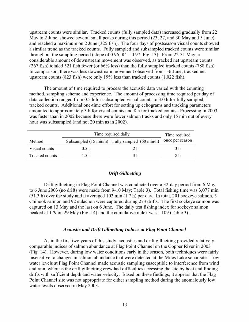
The amount of time required to process the acoustic data varied with the counting method, sampling scheme and experience. The amount of processing time required per day of data collection ranged from 0.5 h for subsampled visual counts to 3.0 h for fully sampled, tracked counts. Additional one-time effort for setting up echograms and tracking parameters amounted to approximately 3 h for visual counts and 8 h for tracked counts. Processing in 2003 was faster than in 2002 because there were fewer salmon tracks and only 15 min out of every hour was subsampled (and not 20 min as in 2002). Time required daily Method Subsampled (15 min/h) Fully sampled (60 min/h)

Time required once per season

Visual counts 0.5 h 2 h 3 h Tracked counts 1.5 h 3 h 8 h

Drift Gillnetting Drift gillnetting in Flag Point Channel was conducted over a 32-day period from 6 May to 6 June 2003 (no drifts were made from 9-10 May; Table 3). Total fishing time was 3,077 min (51.3 h) over the study and it averaged 102 min (1.7 h) per day. In total, 201 sockeye salmon, 5 Chinook salmon and 92 eulachon were captured during 273 drifts. The first sockeye salmon was captured on 13 May and the last on 6 June. The daily test fishing index for sockeye salmon peaked at 179 on 29 May (Fig. 14) and the cumulative index was 1,109 (Table 3).

Acoustic and Drift Gillnetting Indices at Flag Point Channel

As in the first two years of this study, acoustics and drift gillnetting provided relatively comparable indices of salmon abundance at Flag Point Channel on the Copper River in 2003 (Fig. 14). However, during low water conditions early in the season, both techniques were fairly insensitive to changes in salmon abundance that were detected at the Miles Lake sonar site. Low water levels at Flag Point Channel made acoustic sampling susceptible to interference from wind and rain, whereas the drift gillnetting crew had difficulties accessing the site by boat and finding drifts with sufficient depth and water velocity. Based on these findings, it appears that the Flag Point Channel site was not appropriate for either sampling method during the anomalously low water levels observed in May 2003.

13

Relative to the Miles Lake sonar counts (Table C-1) with a 2-day lag, the Flag Point Channel indices showed a less pronounced peak on 22-23 May, and a more pronounced peak on 2 June (Fig. 14). Trends in the acoustic and drift gillnetting indices were similar during these periods suggesting that the differences between the Flag Point Channel and Miles Lake sonar indices were specific to the location rather than to the type of gear used at Flag Point Channel.

Some variation in the Flag Point Channel indices appeared to be related to the length of time the gear types sampled each day. Acoustics sampling occurred 24 hours per day (apart from minor stoppages) for 693 h from 8 May to 6 June. Drift gillnets sampled for 51 h from 6 May to 6 June with sets typically made during daylight hours. From 12 May to 7 June, 203,044 fish were counted at the Miles Lake sonar site. Over the same period (11 May to 6 June to account for 1-d lag), 1,880 fish (0.9% of Miles Lake count) were sampled by the acoustic gear at Flag Point Channel and only 201 fish (0.1% of Miles Lake count) were sampled using drift gillnets. Also, the ratio between acoustic and drift gillnetting indices was three times higher on 2 June than it was on 5 June. A closer inspection of the acoustic counts on these two days revealed that almost half of the fish on 2 June passed the sample site from 0000 to 0600 hours, while fish passage was more evenly distributed throughout the day on 5 June. The fact that no drift gillnetting occurred before 0600 hours on 2 June explains the difference in counts between the sampling methods.

The catch efficiencies (index per 1,000 fish counted at Miles Lake) of acoustics and drift gillnetting were compared by plotting the Flag Point Channel indices as a function of the Miles Lake sonar counts lagged by one day (3-d moving averages; Fig. 15). In the early part of the study period (17-24 May), the catch efficiencies for acoustics (avg. = 2.5) and drift gillnetting (avg. = 4.8) were both relatively low. However, from 25 May to 5 June, the catch efficiency of acoustics (avg. = 11.0) was substantially higher on average than that for drift gillnetting (avg. = 6.2). This latter period coincided with a time of increasing fish passage and stage height. Due to the low and variable fish counts in 2003, the relationship between the catch efficiency of each gear type and stage height was less conclusive than in 2002.

Daily acoustic and drift gillnetting indices at Flag Point Channel decreased 1-2 d after the start of a commercial fishing opening in the Copper River District (Fig. 14), suggesting that salmon migrated from the fishery to Flag Point Channel in about 1-2 d.

Forecasting Miles Lake Sonar Counts Using Flag Point Channel Indices

An examination of the mean percent error revealed a positive bias in the forecasts (i.e., the Flag Point Channel indices overestimated the Miles Lake sonar counts) for both acoustics and drift gillnetting (Fig. 16). In fact, the first 10 to 11 days of forecasts in 2003 were positively biased. Forecasts from drift gillnetting data were slightly more biased than forecasts from acoustic data. The mean error and MPE were smaller for forecasts that used a 2 to 3 day lag instead of a 1 day lag; however, the forecasts appear to be fairly robust to different lag times. The MLE is a special case of regression where the intercept is set equal to zero, and thus the regression produced a better fit model. An examination of the mean absolute percent error showed that forecasts in 2003 were more precise for 2 and 3 day lags than for 1 day lags (Fig. 17). Forecasts from drift gillnetting data were slightly more precise than forecasts from acoustic data.

14

DISCUSSION

Acoustics

Generating salmon counts from acoustic data collected at Flag Point Channel was more difficult in 2003 than in previous years. Unfortunately, the frequency distribution of target strengths did not reveal a clear threshold value that could be used to separate eulachon and salmon. This uncertainty was attributed to two possible factors. First, during the last two weeks in May, the target strength of salmon was lower than expected. This may have been caused by the transducer being aimed too far upstream or downstream, which would have ensonified fish at an oblique angle and thus produce weaker echoes. However, the heading of the transducer was kept constant (± 2°) throughout the entire sampling period. In contrast, the target strength of salmon increased gradually towards the end of May, suggesting it was not caused by any sudden event such as moving or re-aiming the transducer. This change in target strength occurred over roughly the same time period as when the water levels started to increase, so it may have been related to environmental factors. Second, it was also difficult to separate eulachon and salmon because so few salmon were actually sampled in 2003, and there was a high proportion of eulachon tracked relative to salmon. Sensitivity analyses revealed that the acoustic counts were comparable to the test fishing indices despite varying the target strength threshold (-40 and -41 dB).

During the visual review of angle-coded echograms from the second half of May, a considerable number of downstream-moving fish were observed, which suggests there was milling behavior at Flag Point Channel. This was probably due in large part to the extremely low water levels and velocities. This was also reflected in the tracked net upstream counts being significantly lower than the tracked counts. However, tracked counts (i.e., disregarding direction of movement) appeared to be a better predictor of Miles Lake sonar counts than tracked net upstream counts. Fish that returned downstream in Flag Point Channel may have found alternative migration routes.

There was very little difference between fully sampled and subsampled (15 min out of every hour) acoustic counts. Among the sampling schemes and counting methods examined, the subsampled visual and tracked counts were the most cost-effective methods. As in 2002, salmon showed little bottom orientation, but still appeared to be bank oriented despite the low water levels in 2003. Approximately the same number of upstream-moving fish were tracked in the onshore and offshore halves of the counting range. If fish were not bank oriented, more would have been sampled at longer ranges because the sample volume increases geometrically with the spreading beam (and fish showed no vertical preference).

Several new features were added in 2003 to better enable the system to be moved to a new location if the need arises in the future. The Starband internet system allowed Aquacoustics staff elsewhere in Alaska to communicate with the NVE technicians on site and remotely control

15

the acoustic system, access data and fix technical problems. In turn, this significantly reduced the amount of time experienced and highly trained individuals were required on site. The system could be improved in future studies by better aiming the antenna and using a faster modem. The BioSonics DTX acoustics system allowed the data acquisition computer to be moved from the streamside to the trailer, thereby reducing the amount of power required at the streamside by half. Combined with the wind generator and two solar panels added in 2002, the streamside setup was nearly self-sufficient in 2003. The angle of the solar panels should be optimized or a third solar panel should be added in future studies. And lastly, a float switch was mounted on the side of the transducer that turns off the echo sounder when the transducer becomes exposed, thereby preventing damage to its ceramic elements.

NVE staff gained valuable experience in operating and maintaining the acoustic system, which kept the amount of down time to a minimum in 2003. Unfortunately, inseason visual counts were compromised by echogram color settings that were not consistent with the counting rules. This led to a large number of eulachon being included in the salmon counts. Once the error was corrected, visual counts were again similar to tracked counts. This error can be easily avoided in the future by routinely checking the echogram settings. All inseason visual counts were passed on to ADF&G fishery managers in Cordova on time.

Flag Point Channel Indices as a Management Tool

Acoustic and drift gillnetting methods were unable to effectively index the abundance of early-run salmon in the lower Copper River in 2003 or to track the general trends in abundance observed at the Miles Lake sonar site. Unlike the previous two field seasons, anomalously low water levels in May 2003 interfered with all sampling at Flag Point Channel and may have caused fish migration to shift to channels on the east side of the delta. Under these conditions, a fishery manager might interpret a low index value at Flag Point Channel as a sign of low inriver salmon abundance, when in fact a large pulse of fish could be migrating upstream in alternative river channels.

In 2003, the travel time of sockeye salmon from Flag Point Channel to the Miles Lake sonar site appeared to range from 1-3 d (lags of 2-3 d produced the best model fits). These were similar to the travel times observed in 2001 (1-2 d) and 2002 (1-3 d). Again, similar to the previous two years, fish appeared to move quickly (1-2 d) through the 16-km section of the lower Copper River between the Copper River District and Flag Point Channel in 2003. This estimated travel time of salmon migrating from the Copper River District to the Miles Lake sonar site was considerably faster than the 3-9 d travel time believed to occur prior to this study. Clearly, the value of a lower river test fishery as a forecasting tool for fishery managers would be greater in years when the lag time between Flag Point Channel and the Miles Lake sonar site was longer.

Fishery managers recognize two broad but useful levels of precision for escapement data from a lower river test fishery in the Copper River: presence/absence and a more quantitative measure such as “more than a few hundred fish, less than 20,000 fish,” etc. Each year, in the earliest stages of the Copper River District commercial fishery (mid-May), managers simply

16

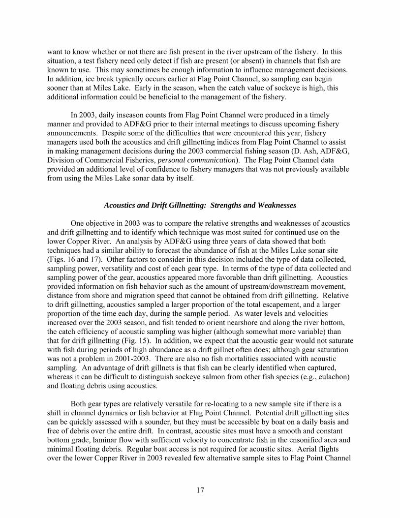
want to know whether or not there are fish present in the river upstream of the fishery. In this situation, a test fishery need only detect if fish are present (or absent) in channels that fish are known to use. This may sometimes be enough information to influence management decisions. In addition, ice break typically occurs earlier at Flag Point Channel, so sampling can begin sooner than at Miles Lake. Early in the season, when the catch value of sockeye is high, this additional information could be beneficial to the management of the fishery.

In 2003, daily inseason counts from Flag Point Channel were produced in a timely

manner and provided to ADF&G prior to their internal meetings to discuss upcoming fishery announcements. Despite some of the difficulties that were encountered this year, fishery managers used both the acoustics and drift gillnetting indices from Flag Point Channel to assist in making management decisions during the 2003 commercial fishing season (D. Ash, ADF&G, Division of Commercial Fisheries, personal communication). The Flag Point Channel data provided an additional level of confidence to fishery managers that was not previously available from using the Miles Lake sonar data by itself.

Acoustics and Drift Gillnetting: Strengths and Weaknesses

One objective in 2003 was to compare the relative strengths and weaknesses of acoustics and drift gillnetting and to identify which technique was most suited for continued use on the lower Copper River. An analysis by ADF&G using three years of data showed that both techniques had a similar ability to forecast the abundance of fish at the Miles Lake sonar site (Figs. 16 and 17). Other factors to consider in this decision included the type of data collected, sampling power, versatility and cost of each gear type. In terms of the type of data collected and sampling power of the gear, acoustics appeared more favorable than drift gillnetting. Acoustics provided information on fish behavior such as the amount of upstream/downstream movement, distance from shore and migration speed that cannot be obtained from drift gillnetting. Relative to drift gillnetting, acoustics sampled a larger proportion of the total escapement, and a larger proportion of the time each day, during the sample period. As water levels and velocities increased over the 2003 season, and fish tended to orient nearshore and along the river bottom, the catch efficiency of acoustic sampling was higher (although somewhat more variable) than that for drift gillnetting (Fig. 15). In addition, we expect that the acoustic gear would not saturate with fish during periods of high abundance as a drift gillnet often does; although gear saturation was not a problem in 2001-2003. There are also no fish mortalities associated with acoustic sampling. An advantage of drift gillnets is that fish can be clearly identified when captured, whereas it can be difficult to distinguish sockeye salmon from other fish species (e.g., eulachon) and floating debris using acoustics.

Both gear types are relatively versatile for re-locating to a new sample site if there is a

shift in channel dynamics or fish behavior at Flag Point Channel. Potential drift gillnetting sites can be quickly assessed with a sounder, but they must be accessible by boat on a daily basis and free of debris over the entire drift. In contrast, acoustic sites must have a smooth and constant bottom grade, laminar flow with sufficient velocity to concentrate fish in the ensonified area and minimal floating debris. Regular boat access is not required for acoustic sites. Aerial flights over the lower Copper River in 2003 revealed few alternative sample sites to Flag Point Channel

17

for either gear type. It appears that finding an alternative sample site (if required) will be more difficult than re-locating the sample gear.

In January 2004, project investigators from NVE, ADF&G, Aquacoustics, Inc. and LGL met in Cordova to discuss the relative merits of both acoustics and drift gillnetting. Based on the information presented at the public workshop (19 January) and contained in this report, acoustics was selected for continued use on the lower Copper River during the 2004 field season.

CONCLUSIONS

1) Anomalously low water conditions in May 2003 interfered with acoustic and drift gillnetting at Flag Point Channel (more so than in previous two seasons);

2) Eulachon were more difficult to distinguish from salmon using acoustics in 2003 than in the previous two seasons;

3) Fish were detected throughout the ensonified water column for most of the counting range, indicating that fish were not bottom-oriented in Flag Point Channel;

4) Lags of 2-3 d between Flag Point Channel and the Miles Lake sonar site produced the best fit models when generating forecasts; and

5) Based on changes in the Flag Point Channel indices, it appeared that fish took 1-2 d to travel the 16-km distance upstream from the Copper River District.

RECOMMENDATIONS It is recommended that the following activities be conducted in 2004:

1) Discontinue drift gillnetting and use acoustics to index salmon abundance at Flag Point Channel; and

2) Continue to monitor the among-year variability of fish behavior at Flag Point Channel and travel times from Flag Point Channel to Miles Lake.

18

ACKNOWLEDGMENTS Special thanks to NVE technicians Rion Schmidt and Joanna Reichhold who conducted the acoustic fieldwork. Iris O’Brien (NVE) provided logistical support that was instrumental to the success of this multi-faceted project. Bruce Cain and Erica McCall Valentine (NVE) also provided valuable project support. We also thank everyone who attended the workshop in Cordova and provided valuable feedback on the project. This project was approved by the Federal Subsistence Board; technical oversight was provided by the USFWS Office of Subsistence Management; and the project was funded by the US Forest Service. The project was a cooperative effort between the US Forest Service (USFS), Native Village of Eyak, Alaska Department of Fish and Game, Aquacoustics, Inc. and LGL Alaska Research Associates, Inc. This annual report partially fulfills contract obligations for USFS Contract #53-0109-2-00593.

19

LITERATURE CITED Brabets, T. P. 1997. Geomorphology of the lower Copper River, Alaska. United States Geological Survey, U.S. Geological Survey Professional Paper 1581, Denver, CO. Burgner, R. L. 1991. Life history of sockeye salmon (Oncorhynchus nerka). p. 1-116 In Pacific salmon life histories. Ed. Groot, C. and Margolis, L. UBC Press, Vancouver. Gray, D., D. Ashe, J. Johnson, R. Merizon, and S. Moffitt. 2002. Prince William Sound Management Area, 2001 Annual Finfish Management Report. Alaska Department of Fish and Game, Commercial Fisheries Division, Regional Information Report No. 2A02-20, Anchorage. Gray, D. C. 2000. Bristol Bay sockeye salmon spawning escapement test fishing, 1999. Alaska Department of Fish and Game, Division of Commercial Fisheries, Regional Information Report No. 2A-00-28, Anchorage. Lambert, M. B., D. Degan, A. M. Mueller, S. Moffitt, B. Marston, N. Gove, and J. J. Smith. 2003. Assessing methods to index inseason salmon abundance in the lower Copper River, 2002 Annual Report. US Fish and Wildlife Service, Office of Subsistence Management, Fisheries Resource Monitoring Program, Annual Report No. FIS 01-021, Anchorage. Link, M. R., B. Haley, D. Degan, A. M. Mueller, S. Moffitt, N. Gove, and R. Henrichs. 2001. Assessing methods to estimate inseason salmon abundance in the lower Copper River. U.S. Fish and Wildlife Service, Office of Subsistence Management, Fisheries Resource Monitoring Program, Annual Report No. FIS01-02101, Anchorage, Alaska. Merritt, M. F., and K. Roberson. 1986. Migratory timing of upper Copper River sockeye salmon stocks and its implications for the regulation of the commercial fishery. N. Amer. J. Fish. Manag. 6: 216-225. Moffitt, S., M. Miller, and B. Mulligan. 2000. Copper River test fishery summary. Alaska Department of Fish and Game, Commercial Fisheries Division, Cordova. Roberson, K., F. H. Bird, K. A. Webster, and P. J. Fridgen. 1980. Copper River-Prince William Sound sockeye salmon catalog and inventory. Anadromous Fish Conservation Act Project No. AFC-61-2. Schaller, H. A. 1984. Determinants for the timing of escapement from the sockeye salmon fishery of the Copper River, Alaska: a simulation model. Department of Oceanography, Old Dominion University, Technical Report No. 84-5, Virginia. Taube, T., and D. Sarafin. 2001. Area management report for the recreational fisheries of the Upper Copper/Upper Susitna River management area, 1999. Alaska Department of Fish and Game, Division of Sport Fish, Fishery Management Report No. 01-7, Anchorage, AK.

20

FIGURES

21

Figure 1. Map of the lower Copper River in Alaska showing the location of Flag Point Channel and the Miles Lake sonar site, 2003.

22

Figure 2. Bathymetry of the acoustic sampling site used in 2002 and 2003 which was located at Flag Point Channel 400 m downstream of Bridge 331 on the Copper River Highway.

23

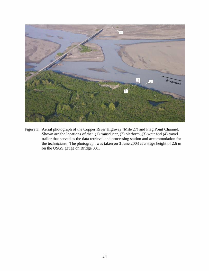
Figure 3. Aerial photograph of the Copper River Highway (Mile 27) and Flag Point Channel. Shown are the locations of the: (1) transducer, (2) platform, (3) weir and (4) travel trailer that served as the data retrieval and processing station and accommodation for the technicians. The photograph was taken on 3 June 2003 at a stage height of 2.6 m on the USGS gauge on Bridge 331.

24

Figure 4. Design of the transducer mount showing the location of the (1) transducer, (2) attitude sensor, (3) float switch, (4) setscrews for adjusting the vertical position and (5) tilt angle of the transducer.

25

Figure 5. Platform for the streamside equipment which consisted of (1) a fish tote that housed the DTX echosounder, wireless Ethernet bridge, fuse bank, battery bank, charger and charge controller, (2) a wireless Ethernet antenna, (3) a wind generator and (4) the solar panels.

26

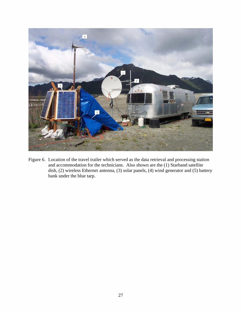
Figure 6. Location of the travel trailer which served as the data retrieval and processing station and accommodation for the technicians. Also shown are the (1) Starband satellite dish, (2) wireless Ethernet antenna, (3) solar panels, (4) wind generator and (5) battery bank under the blue tarp.

27

Figure 7. Frequency distribution of the average target strength of fish tracked at Flag Point Channel on the Copper River, 2003.

0

100

200

300

400

500

-54 -50 -46 -42 -38 -34 -30 -26 -22

Average target strength (dB)

Num

ber o

f tra

cks

Eulachon

Salmon

28

Figure 8. Daily average and daily maximum of the average target strength of fish tracked at Flag Point Channel on the Copper River, 2003.

-50

-40

-30

-20

-10

0

08-May 12-May 16-May 20-May 24-May 28-May 01-Jun 05-Jun

Targ

et st

reng

th (d

B)

Average of average TSMaximum of average TS

29

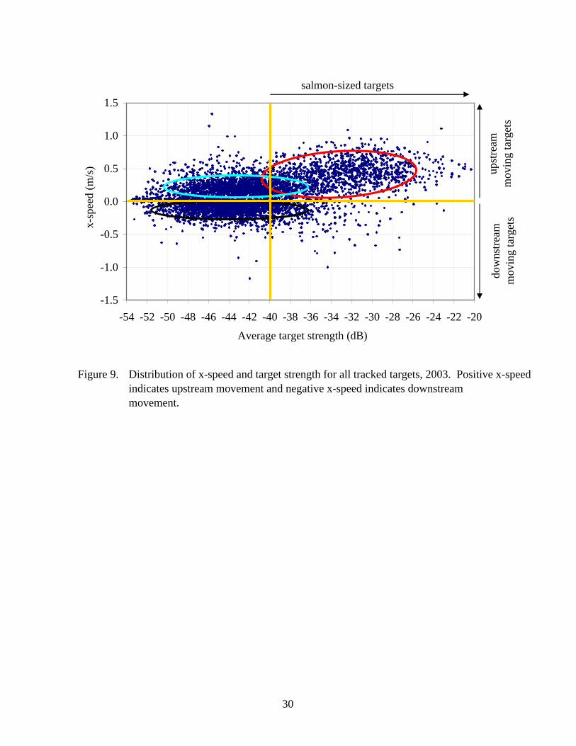
Figure 9. Distribution of x-speed and target strength for all tracked targets, 2003. Positive x-speed indicates upstream movement and negative x-speed indicates downstream movement.

-1.5

-1.0

-0.5

0.0

0.5

1.0

1.5

-54 -52 -50 -48 -46 -44 -42 -40 -38 -36 -34 -32 -30 -28 -26 -24 -22 -20

Average target strength (dB)

x-sp

eed

(m/s

)salmon-sized targets

upst

ream

m

ovin

g ta

rget

sdo

wns

tream

m

ovin

g ta

rget

s

30

Figure 10. Profile of the river bottom and vertical distribution of fish over range at the acoustic sampling site at Flag Point Channel, 2003. All range data is referenced to the transducer position used from May 31 to the end of the season.

16

17

18

19

20

21

22

0 4 8 12 16 20 24 28 32 36

Distance (m)

Elev

atio

n (m

)Right Bank

Profile of river bank (May 2003)Profile of river bottom (May 2002)Vertical position and range of tracked fishTransducer and acoustic beam

31

Figure 11. Direction of movement and range of salmon-sized targets that were tracked at Flag Point Channel on the Copper River, 2003. All range data is referenced to the transducer position used from 31 May to the end of the season.

0

40

80

120

160

200

0 1 2 3 4 5 6 7 8 9 10 11 12 13 14Range (m)

Num

ber o

f fis

hUpstream moving salmonDownstream moving salmon

32

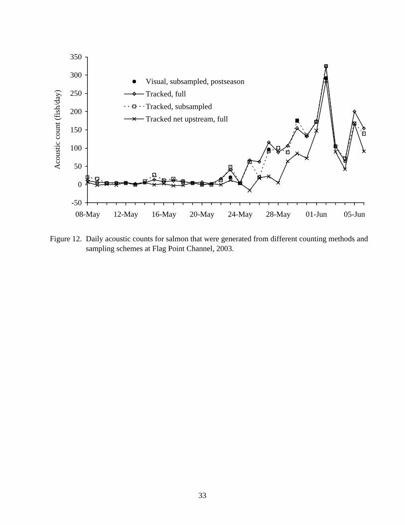
Figure 12. Daily acoustic counts for salmon that were generated from different counting methods and sampling schemes at Flag Point Channel, 2003.

-50

0

50

100

150

200

250

300

350

08-May 12-May 16-May 20-May 24-May 28-May 01-Jun 05-Jun

Aco

ustic

cou

nt (f

ish/

day)

Visual, subsampled, postseasonTracked, fullTracked, subsampledTracked net upstream, full

33

Figure 13. Linear regression of full and subsampled tracked counts for salmon at Flag Point Channel on the Copper River, 2003.

y = 0.96x + 0.48R2 = 0.97

0

50

100

150

200

250

300

350

0 50 100 150 200 250 300 350

Full tracked counts (fish/day)

Subs

ampl

ed tr

acke

d co

unts

(fis

h/da

y)

34

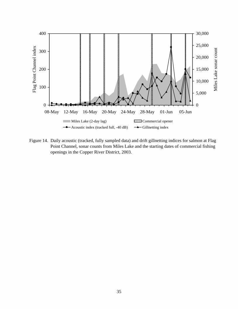
Figure 14. Daily acoustic (tracked, fully sampled data) and drift gillnetting indices for salmon at Flag Point Channel, sonar counts from Miles Lake and the starting dates of commercial fishing openings in the Copper River District, 2003.

0

100

200

300

400

08-May 12-May 16-May 20-May 24-May 28-May 01-Jun 05-Jun

Flag

Poi

nt C

hann

el in

dex

0

5,000

10,000

15,000

20,000

25,000

30,000

Mile

s Lak

e so

nar c

ount

Miles Lake (2-day lag) Commercial openerAcoustic index (tracked full, -40 dB) Gillnetting index

35

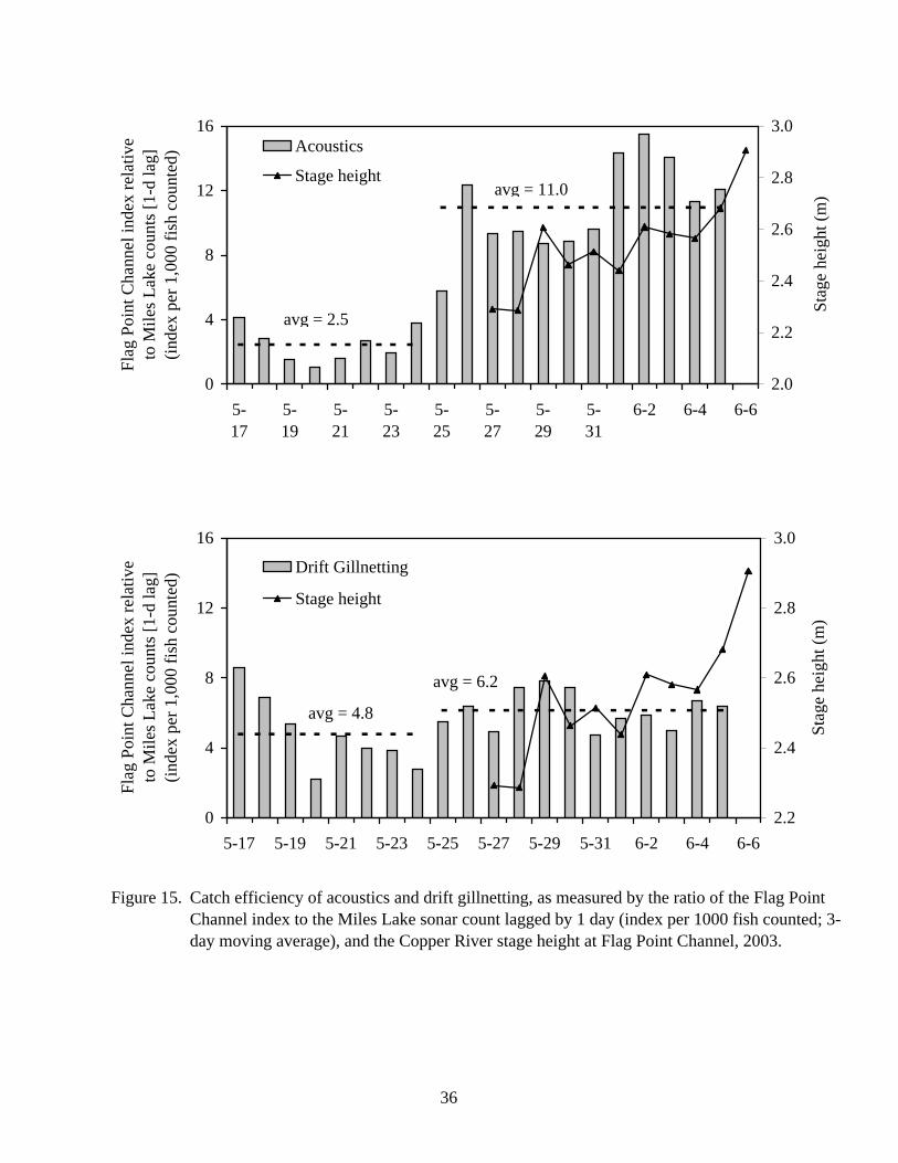
Figure 15. Catch efficiency of acoustics and drift gillnetting, as measured by the ratio of the Flag Point Channel index to the Miles Lake sonar count lagged by 1 day (index per 1000 fish counted; 3-day moving average), and the Copper River stage height at Flag Point Channel, 2003.

0

4

8

12

16

5-17

5-19

5-21

5-23

5-25

5-27

5-29

5-31

6-2 6-4 6-6

Flag

Poi

nt C

hann

el in

dex

rela

tive

to M

iles L

ake

coun

ts [1

-d la

g]

(inde

x pe

r 1,0

00 fi

sh c

ount

ed)

2.0

2.2

2.4

2.6

2.8

3.0

Stag

e he

ight

(m)

Acoustics

Stage height

avg = 2.5

avg = 11.0

0

4

8

12

16

5-17 5-19 5-21 5-23 5-25 5-27 5-29 5-31 6-2 6-4 6-6

Flag

Poi

nt C

hann

el in

dex

rela

tive

to M

iles L

ake

coun

ts [1

-d la

g]

(inde

x pe

r 1,0

00 fi

sh c

ount

ed)

2.2

2.4

2.6

2.8

3.0

Stag

e he

ight

(m)

Drift Gillnetting

Stage height

avg = 4.8

avg = 6.2

36

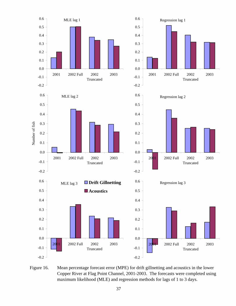
Figure 16. Mean percentage forecast error (MPE) for drift gillnetting and acoustics in the lower Copper River at Flag Point Channel, 2001-2003. The forecasts were completed using maximum likelihood (MLE) and regression methods for lags of 1 to 3 days.

MLE lag 1

-0.2

-0.1

0.0

0.1

0.2

0.3

0.4

0.5

0.6

2001 2002 Full 2002Truncated

2003

Regression lag 1

-0.2

-0.1

0.0

0.1

0.2

0.3

0.4

0.5

0.6

2001 2002 Full 2002Truncated

2003

MLE lag 2

-0.2

-0.1

0.0

0.1

0.2

0.3

0.4

0.5

0.6

2001 2002 Full 2002Truncated

2003

Num

ber o

f fis

h

Regression lag 2

-0.2

-0.1

0.0

0.1

0.2

0.3

0.4

0.5

0.6

2001 2002 Full 2002Truncated

2003

MLE lag 3

-0.2

-0.1

0.0

0.1

0.2

0.3

0.4

0.5

0.6

2001 2002 Full 2002Truncated

2003

Drift Gillnetting

Acoustics

Regression lag 3

-0.2

-0.1

0.0

0.1

0.2

0.3

0.4

0.5

0.6

2001 2002 Full 2002Truncated

2003

37

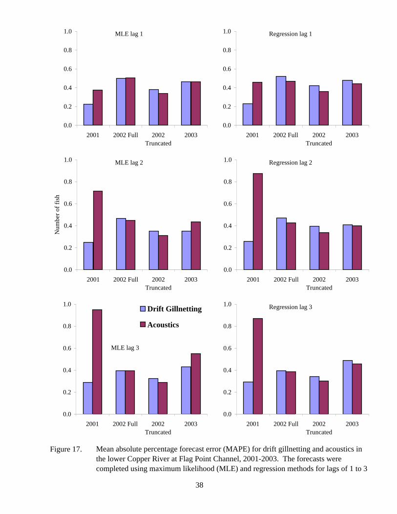
Figure 17. Mean absolute percentage forecast error (MAPE) for drift gillnetting and acoustics in the lower Copper River at Flag Point Channel, 2001-2003. The forecasts were completed using maximum likelihood (MLE) and regression methods for lags of 1 to 3

MLE lag 1

0.0

0.2

0.4

0.6

0.8

1.0

2001 2002 Full 2002Truncated

2003

Regression lag 1

0.0

0.2

0.4

0.6

0.8

1.0

2001 2002 Full 2002Truncated

2003

MLE lag 2

0.0

0.2

0.4

0.6

0.8

1.0

2001 2002 Full 2002Truncated

2003

Num

ber o

f fis

h

Regression lag 2

0.0

0.2

0.4

0.6

0.8

1.0

2001 2002 Full 2002Truncated

2003

MLE lag 3

0.0

0.2

0.4

0.6

0.8

1.0

2001 2002 Full 2002Truncated

2003

Drift Gillnetting

Acoustics

Regression lag 3

0.0

0.2

0.4

0.6

0.8

1.0

2001 2002 Full 2002Truncated

2003

38

APPENDICES

43

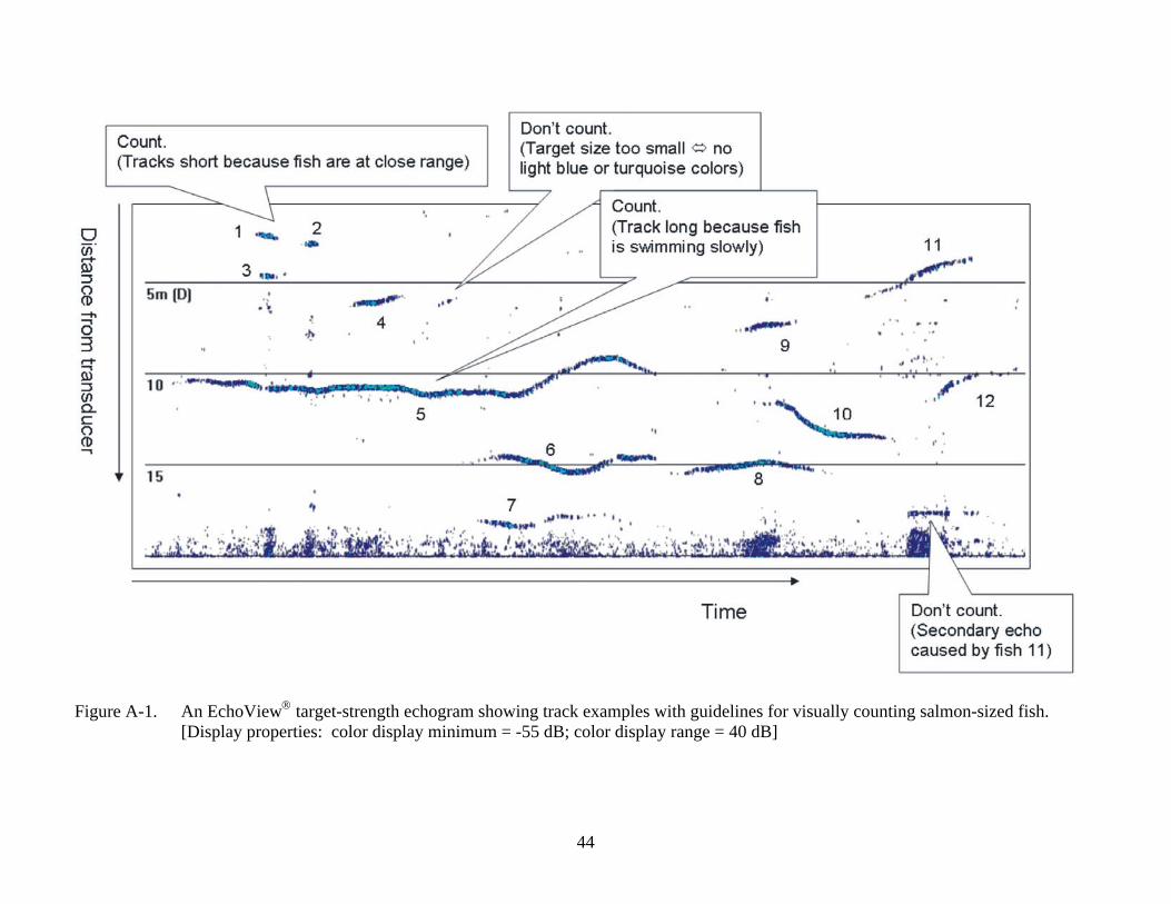
Figure A-1. An EchoView® target-strength echogram showing track examples with guidelines for visually counting salmon-sized fish. [Display properties: color display minimum = -55 dB; color display range = 40 dB]

44

Figure A-2. An EchoView® angle echogram showing track examples with guidelines distinguishing a disrupted track caused by a single fish from tracks caused by multiple fish. Targets in cool colors are on the downstream side of the transducer, targets in warm colors are on the upstream side of the transducer. [Display properties: major axis angle range = ± 8o; major axis color scheme = DT4; minor axis color scheme = none]

45

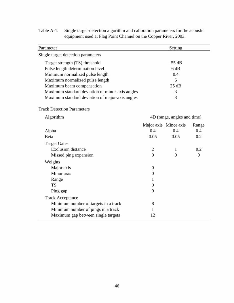
Table A-1. Single target-detection algorithm and calibration parameters for the acoustic equipment used at Flag Point Channel on the Copper River, 2003.

Parameter SettingSingle target detection parameters

Target strength (TS) threshold -55 dBPulse length determination level 6 dBMinimum normalized pulse length 0.4Maximum normalized pulse length 5Maximum beam compensation 25 dBMaximum standard deviation of minor-axis angles 3Maximum standard deviation of major-axis angles 3

Track Detection Parameters

Algorithm 4D (range, angles and time)

Major axis Minor axis RangeAlpha 0.4 0.4 0.4Beta 0.05 0.05 0.2Target Gates

Exclusion distance 2 1 0.2Missed ping expansion 0 0 0

WeightsMajor axis 0Minor axis 0Range 1TS 0Ping gap 0

Track AcceptanceMinimum number of targets in a track 8Minimum number of pings in a track 1Maximum gap between single targets 12

46

Figure B-1. Stage height of the Copper River at Flag Point Channel and the Million Dollar Bridge, 2003.

2.1

2.3

2.5

2.7

2.9

3.1

5-8 5-11 5-14 5-17 5-20 5-23 5-26 5-29 6-1 6-4 6-7

Stag

e he

ight

(m) a

t Fla

g Po

int C

hann

el

39.0

39.5

40.0

40.5

41.0

Stag

e he

ight

(m) a

t the

M

illio

n D

olla

r Brid

ge

Flag Point Channel - West BridgeFlag Point Channel - East BridgeMillion Dollar Bridge

47

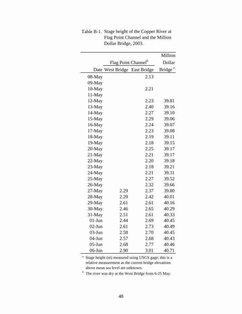
Table B-1.

MillionDollar

Date West Bridge East Bridge Bridge a

08-May 2.1309-May10-May 2.2111-May12-May 2.23 39.8113-May 2.40 39.1614-May 2.27 39.1015-May 2.29 39.0616-May 2.24 39.0717-May 2.23 39.0818-May 2.19 39.1119-May 2.18 39.1520-May 2.25 39.1721-May 2.21 39.1722-May 2.20 39.1823-May 2.18 39.2124-May 2.21 39.3125-May 2.27 39.5226-May 2.32 39.6627-May 2.29 2.37 39.8028-May 2.29 2.42 40.0129-May 2.61 2.61 40.1630-May 2.46 2.65 40.2931-May 2.51 2.61 40.3301-Jun 2.44 2.69 40.4502-Jun 2.61 2.73 40.4903-Jun 2.58 2.70 40.4504-Jun 2.57 2.68 40.4305-Jun 2.68 2.77 40.4606-Jun 2.90 3.01 40.71

a

b The river was dry at the West Bridge from 6-25 May.

Flag Point Channel b

Stage height (m) measured using USGS gage; this is a relative measurement as the current bridge elevations above mean sea level are unknown.

Stage height of the Copper River at Flag Point Channel and the Million Dollar Bridge, 2003.

48

Table C-1. Daily salmon counts and escapement objectives at the Miles Lake sonar, 2003.

Stageheight North South

Date (m) a Bank Bank Daily Cum. Daily Cum.12-May 39.81 0 0 013-May 39.16 81 81 8114-May 39.10 187 250 437 51815-May 39.06 280 381 661 1,179 0 016-May 39.07 304 915 1,219 2,398 17 1717-May 39.08 432 1,163 1,595 3,993 382 39918-May 39.11 272 1,178 1,450 5,443 911 1,31019-May 39.15 960 2,563 3,523 8,966 1,264 2,57420-May 39.17 832 2,604 3,436 12,402 1,415 3,98921-May 39.17 832 4,544 5,376 17,778 1,478 5,46722-May 39.18 672 3,178 3,850 21,628 1,973 7,44023-May 39.21 640 4,849 5,489 27,117 2,823 10,26324-May 39.31 544 11,535 12,079 39,196 4,316 14,57925-May 39.52 1,480 11,621 13,101 52,297 4,397 18,97626-May 39.66 944 3,053 3,997 56,294 4,593 23,56927-May 39.80 1,464 4,421 5,885 62,179 6,589 30,15828-May 40.01 881 9,049 9,930 72,109 8,637 38,79529-May 40.16 816 11,961 12,777 84,886 6,159 44,95430-May 40.29 536 9,502 10,038 94,924 7,330 52,28431-May 40.33 696 16,436 17,132 112,056 9,751 62,03501-Jun 40.45 336 16,942 17,278 129,334 10,138 72,17302-Jun 40.49 288 13,149 13,437 142,771 11,464 83,63703-Jun 40.45 160 13,004 13,164 155,935 11,049 94,68604-Jun 40.43 288 12,083 12,371 168,306 12,535 107,22105-Jun 40.46 184 9,262 9,446 177,752 13,792 121,01306-Jun 40.71 128 10,692 10,820 188,572 12,457 133,47107-Jun 40.98 272 14,200 14,472 203,044 12,236 145,70708-Jun 41.23 648 15,711 16,359 219,403 14,192 159,89909-Jun 41.29 1,112 16,303 17,415 236,818 13,581 173,48010-Jun 41.35 2,088 11,863 13,951 250,769 13,013 186,49311-Jun 41.61 2,264 18,585 20,849 271,618 12,577 199,07012-Jun 41.93 816 18,230 19,046 290,664 11,659 210,72913-Jun 42.25 1,568 10,994 12,562 303,226 10,271 221,00014-Jun 42.53 1,104 11,186 12,290 315,516 9,896 230,89615-Jun 42.67 408 10,459 10,867 326,383 10,615 241,51216-Jun 42.48 496 12,525 13,021 339,404 9,600 251,11217-Jun 42.25 864 12,583 13,447 352,851 9,612 260,724

Estimated daily escapement Escapementobjective

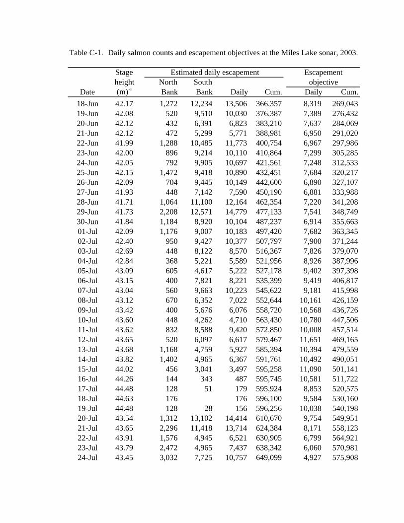
Table C-1. Daily salmon counts and escapement objectives at the Miles Lake sonar, 2003.

Stageheight North South

Date (m) a Bank Bank Daily Cum. Daily Cum.

Estimated daily escapement Escapementobjective

18-Jun 42.17 1,272 12,234 13,506 366,357 8,319 269,04319-Jun 42.08 520 9,510 10,030 376,387 7,389 276,43220-Jun 42.12 432 6,391 6,823 383,210 7,637 284,06921-Jun 42.12 472 5,299 5,771 388,981 6,950 291,02022-Jun 41.99 1,288 10,485 11,773 400,754 6,967 297,98623-Jun 42.00 896 9,214 10,110 410,864 7,299 305,28524-Jun 42.05 792 9,905 10,697 421,561 7,248 312,53325-Jun 42.15 1,472 9,418 10,890 432,451 7,684 320,21726-Jun 42.09 704 9,445 10,149 442,600 6,890 327,10727-Jun 41.93 448 7,142 7,590 450,190 6,881 333,98828-Jun 41.71 1,064 11,100 12,164 462,354 7,220 341,20829-Jun 41.73 2,208 12,571 14,779 477,133 7,541 348,74930-Jun 41.84 1,184 8,920 10,104 487,237 6,914 355,66301-Jul 42.09 1,176 9,007 10,183 497,420 7,682 363,34502-Jul 42.40 950 9,427 10,377 507,797 7,900 371,24403-Jul 42.69 448 8,122 8,570 516,367 7,826 379,07004-Jul 42.84 368 5,221 5,589 521,956 8,926 387,99605-Jul 43.09 605 4,617 5,222 527,178 9,402 397,39806-Jul 43.15 400 7,821 8,221 535,399 9,419 406,81707-Jul 43.04 560 9,663 10,223 545,622 9,181 415,99808-Jul 43.12 670 6,352 7,022 552,644 10,161 426,15909-Jul 43.42 400 5,676 6,076 558,720 10,568 436,72610-Jul 43.60 448 4,262 4,710 563,430 10,780 447,50611-Jul 43.62 832 8,588 9,420 572,850 10,008 457,51412-Jul 43.65 520 6,097 6,617 579,467 11,651 469,16513-Jul 43.68 1,168 4,759 5,927 585,394 10,394 479,55914-Jul 43.82 1,402 4,965 6,367 591,761 10,492 490,05115-Jul 44.02 456 3,041 3,497 595,258 11,090 501,14116-Jul 44.26 144 343 487 595,745 10,581 511,72217-Jul 44.48 128 51 179 595,924 8,853 520,57518-Jul 44.63 176 176 596,100 9,584 530,16019-Jul 44.48 128 28 156 596,256 10,038 540,19820-Jul 43.54 1,312 13,102 14,414 610,670 9,754 549,95121-Jul 43.65 2,296 11,418 13,714 624,384 8,171 558,12322-Jul 43.91 1,576 4,945 6,521 630,905 6,799 564,92123-Jul 43.79 2,472 4,965 7,437 638,342 6,060 570,98124-Jul 43.45 3,032 7,725 10,757 649,099 4,927 575,908

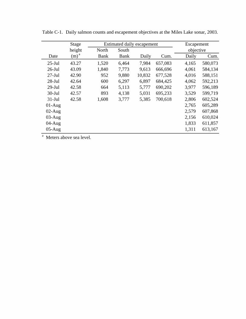
Table C-1. Daily salmon counts and escapement objectives at the Miles Lake sonar, 2003.

Stageheight North South

Date (m) a Bank Bank Daily Cum. Daily Cum.

Estimated daily escapement Escapementobjective

25-Jul 43.27 1,520 6,464 7,984 657,083 4,165 580,07326-Jul 43.09 1,840 7,773 9,613 666,696 4,061 584,13427-Jul 42.90 952 9,880 10,832 677,528 4,016 588,15128-Jul 42.64 600 6,297 6,897 684,425 4,062 592,21329-Jul 42.58 664 5,113 5,777 690,202 3,977 596,18930-Jul 42.57 893 4,138 5,031 695,233 3,529 599,71931-Jul 42.58 1,608 3,777 5,385 700,618 2,806 602,524

01-Aug 2,765 605,28902-Aug 2,579 607,86803-Aug 2,156 610,02404-Aug 1,833 611,85705-Aug 1,311 613,167

a Meters above sea level.

The U.S. Fish and Wildlife Service, Office of Subsistence Management conducts all programs and activities free from discrimination on the basis of sex, color, race, religion, national origin, age, marital status, pregnancy, parenthood or disability. For information on alternative formats available for this publication please contact the office of Subsistence Management to make necessary arrangements. Any person who believes she or he has been discriminated against should write to: Office of Subsistence Management, 3601 C Street, Suite 1030, Anchorage, AK 99503; or O.E.O., U.S. Department of Interior, Washington, D.C. 20240.