assessing gdp and in ation probability forecasts derived

Assessing GDP and Inflation Probability Forecasts

Derived from the Bank of England Fan Charts

John W. GalbraithDepartment of Economics, McGill University

Simon van Norden ∗

Finance, HEC Montreal

June 18, 2012

Abstract

Density forecasts, including the pioneering Bank of England ‘fan charts’, areoften used to produce forecast probabilities of a particular event. We use the Bankof England’s forecast densities to calculate the forecast probability that annual ratesof inflation and output growth exceed given thresholds. We subject these implicitprobability forecasts to a number of graphical and numerical diagnostic checks.We measure both their calibration and their resolution, providing both statisticaland graphical interpretations of the results. The results reinforce earlier evidenceon limitations of these forecasts and provide new evidence on their informationcontent and on the relative performance of inflation and GDP growth forecasts. Inparticular, GDP forecasts show little or no ability to predict periods of low growthbeyond the current quarter, due in part to the important role of data revisions.

Key words: calibration, density forecast, probability forecast, resolution, sharpness

∗We thank Malte Knuppel, Ken Wallis and conference and seminar participants at the Bank ofEngland, Federal Reserve Bank of Philadelphia and the Reserve Bank of New Zealand for valuablecomments. and Rashmi Harimohan of the Bank of England for his technical assistance in repro-ducing the Bank of England’s own probability forecasts. We also thank the Fonds quebecois dela recherche sur la societe et la culture (FQRSC), the Social Sciences and Humanities ResearchCouncil of Canada (SSHRC) and CIRANO (Centre Interuniversitaire de recherche en analyse desorganisations) for support of this research.

1

1. Introduction

Forecasts of the probability that a specific event will occur have attracted increasing

recent interest; see Gneiting (2008) for a discussion and overview. While many series of such

probability forecasts have been subject to careful evaluation (particularly in meteorological

contexts), important economic series have received less precise attention. The present paper

addresses one well known source of economic probability forecasts, arising from the Bank

of England’s fan charts, and subjects them to a number of diagnostic checks. We examine

both inflation and gross domestic product (GDP) growth forecasts; the latter are particularly

important, because much economic behaviour (such as investment, hiring, major purchasing

decisions) is influenced by expectations of near-term growth. One noteworthy finding is that

the GDP growth forecasts have little ability, beyond that of the unconditional distribution

of GDP growth, to distinguish high- and low- probability growth outcomes.

Since their introduction in the 1993 Inflation Report, the Bank of England’s probability

density forecasts (“fan charts”) for inflation, and later output growth, have been studied

by a number of authors. Wallis (2003, 2004) and Clements (2004) studied the inflation

forecasts and concluded that while the current and next-quarter forecast seemed to fit well,

the year-ahead forecasts significantly overestimated the probability of high inflation rates.

Elder, Kapetanios, Taylor and Yates (2005) found similar results for the inflation forecasts,

but also found significant evidence that the GDP growth forecasts do not accurately capture

the true distribution of risks to output growth at very short horizons. Noting the hazards of

drawing firm conclusions from small samples, these authors suggested that “the fan charts

gave a reasonably good guide to the probabilities and risks facing the MPC [monetary policy

committee].” They also explored the role of GDP revisions in accounting for GDP forecast

errors and noted that the dispersion associated with predicted GDP outcomes was increased

as a result of their research. Dowd (2007) concluded that uncertainty in inflation was

substantially overestimated, and Gneiting and Ranjan (2011) reached a similar conclusion

with respect to longer-horizon forecasts in particular. Dowd (2008) examined the GDP fan

charts and found that while short-horizon forecasts appear to capture the risks to output

growth poorly, results for longer horizon forecasts are sensitive to the vintage of data used

to evaluate the forecasts, a point to which we will return below.

Throughout this evaluative work, the focus has been on whether the risks implied by

the Bank’s fan charts are well matched (in a statistical sense) by the frequency of the

various inflation and output growth outcomes. Gneiting, Balabdaoui and Raftery (2007)

refer to this property as ‘probabilistic calibration’. As we will see below, it is well known

that different density functions may satisfy this correct calibration property yet convey

quite different amounts of information; see Corradi and Swanson (2006) and Mitchell and

Wallis (2011) for a discussion. Mitchell and Wallis note that this extra information has

been referred to as ‘sharpness’, ‘refinement’ or ‘resolution’ in various contexts and note its

relationship to the Kullback-Leibler Information Criterion. Although forecast sharpness or

resolution is desirable, no empirical studies of the Bank’s density forecasts have investigated

this property.

Instead of the full forecast density, we work with the implied probabilistic forecasts:

2

we compute the forecast probabilities of failing to achieve the Bank’s inflation target, or

of GDP growth falling below a fixed threshold. (The methods that we use to do so can of

course be applied to probability forecasts for other thresholds simply by integrating under

different regions of the density forecast; different choices of threshold allow one to focus

on different parts of the forecast distribution.) This is similar in spirit to Clements’ (2004)

examination of the fan chart’s implied interval forecasts. The Bank of England also examines

such interval forecasts from time to time; see for example Table 1 (p. 47) of the August

2008 Inflation Report. We investigate both the calibration of the probabilistic forecasts (the

degree to which predicted probabilities correspond with true probabilities of the outcomes),

and their resolution (their ability to discriminate among different outcomes).

In contrast with earlier evaluations, our results provide strong evidence of a mis-calibration

of the inflation forecasts at very short horizons, even though the degree of mis-calibration

appears to be small. Despite the much shorter sample available for the GDP forecasts,

we again find significant evidence of mis-calibration and its magnitude appears to be much

larger than for inflation. Results on the discriminatory power of the forecasts shows that

inflation forecasts appear to have important power to distinguish high- and low- probability

cases up to horizons of about one year. Perhaps most importantly we find that the resolution

of the GDP forecasts, upon which many important decisions are based, is almost negligible

beyond a one-quarter horizon.

2. Data and forecasts

The Bank of England’s Inflation Report provides density forecasts of inflation and,

more recently, output growth in the form of ‘fan charts’. Fan charts for RPIX (retail prices

index excluding mortgage payments) inflation were published from 1993Q1 to 2004Q1, when

they were replaced by CPI (consumer price index) inflation fan charts. Both measure

inflation as the percentage change in the corresponding price index over four quarters. See

Wallis (1999) for a careful discussion of the interpretation of these charts; note in particular

that the different bands do not correspond straightforwardly with quantiles in the general,

asymmetric, case. The GDP fan chart was first published in the 1997Q3 report and also

forecasts the total percentage growth over 4 quarters. In addition to providing forecast

distributions for roughly 0 to 8 quarters into the future, from the 1998Q1 Inflation Report

onwards forecasts are provided conditional on the assumption of either fixed interest rates

or a “market-expectation-based” interest rate profile; the two assumptions typically provide

similar results, and below we will present results for the market interest rate case only

(results for fixed interest rate forecasts are qualitatively very similar). Construction of

probability forecasts from the Bank’s fan charts is described in the Appendix.

For both inflation and GDP growth, we use all available forecasts up to and including

that published in 2010Q1. We measure inflation and output growth outcomes using the

2010Q1 vintage data series, and for GDP we also use the unrevised first estimates of annual

GDP growth.

Taking account of data revision can change materially the apparent performance of GDP

growth forecasts. While inflation (or price level) data are not revised to any substantial

extent, revisions in GDP growth are often comparable in magnitude to GDP growth itself.

3

If our aim in forecasting GDP growth is to predict the actual change in national output (as

opposed to predicting the next initial estimate) then we wish to evaluate performance by the

best estimate of that actual change, i.e. by the latest, last-revised number. Forecasters do

not have the benefit of this latest revision, of course. Working as they do with preliminary

data, they may sometimes produce forecasts which have some predictive power for the next

preliminary data points, but very little for the final estimates of those data points. Below

we present evidence of this phenomenon in the Bank of England (BoE) forecasts.

We report results for nine horizons, zero (the ’nowcast’ for the current quarter) through

eight.

Figure 1 is intended to convey some descriptive information about the probability fore-

cast series with which we work. The left-hand and middle panels of the figure (the right-hand

panels are described below) show the implications of the BoE’s density forecasts for the prob-

abilities that annual real GDP growth is less than the 2.5% threshold mentioned above, and

that annual inflation (based on RPIX or CPI) is less than the Bank’s target value. Note

that the Bank has a scalar target value as well as a band within which inflation outcomes

are considered acceptable; we present results based on each of these indicators below.

Each point in these panels corresponds with the implied forecast probability (on the

vertical axis) that inflation or output growth will be less than the chosen threshold, at the

forecast horizon given on the horizontal axis. The ‘+’ symbols represent cases where the

outcome for which the probability is forecast occurred (e.g. forecast is of probability of

falling below a threshold, and the eventual outcome was below the threshold), while the

circles are cases in which the outcome did not occur. One clearly observable feature is

that the dispersion of these forecasts declines with increasing horizon, as is appropriate; the

declining value of conditioning information with lengthening horizon makes it more difficult

to distinguish high-probability and low-probability states.

Ideal forecasts would have assigned probability one to all the ‘+’s and probability zero

to the circles. Instead, for GDP growth we observe several high probability circles and low

probability ‘+’s (see horizons 2-4 in particular). We also find most outcomes clustered in

the center of the probability range at horizons 4-8. The probabilistic outcomes for inflation

show similar features with respect to changes across horizons, but at the shorter horizons

we see a more marked concentration of ‘+’s at the higher probabilities and of circles at the

lower, suggesting that the inflation forecasts had more discriminatory power than the GDP

forecasts, at least at the short horizons. Below we will present direct evidence on this point.

In the next section, we review some of the literature on density forecast evaluation

before focusing on tests of probabilistic forecasts and properties of forecast calibration and

resolution or sharpness.

4

3. Probability forecast evaluation

3.1 Predictive densities

Let X be a random variable with realizations xt and with probability density and

cumulative distribution functions fX(x) and FX(x) respectively. Then for a given sample

{xt}Tt=1, the corresponding sample of values of the CDF, {FX(xt)}Tt=1, is a U(0,1) sequence.

This well-known result (often termed the probability integral transform of {xt}Tt=1) is the

basis of much predictive density testing, following pioneering work by Diebold, Gunther

and Tay (1998). These authors noted that if the predictive density fX(x) is equal to the

true density, then using the predictive density for the probability integral transform should

produce the same result, i.e. a U(0,1) sequence. This allows us to test whether a given

sequence of forecast densities could be equal to the true sequence by checking whether

{FX(xt)}Tt=1 (i.e. the sequence of CDFs of the realized values using the forecast densities)

is U(0,1).

The right-hand panels of Figure 1 show histograms of the probability integral transforms

(PIT’s) for the Bank’s GDP growth and inflation forecasts. As these are U(0,1) under the

null of correct specification of the conditional density, the histograms should show roughly

the same proportion of observed forecasts in each of the ten cells. In order to represent

compactly the results for nine forecast horizons (0–8 inclusive) in each part of the figure,

we have indicated the outcomes with a colour coding; each row of the figure represents a

different horizon, and each column a particular bin with width 0.1. Uniformly distributed

results would imply a frequency of 0.1 in each bin, and therefore a uniform colour in the

figure. Values well below 0.1 show up as dark blue, and well above 0.1 as red.

While some sampling variation is inevitable, the results are far from uniformity. GDP

growth forecasts often show an excessive number of values in the highest cell (near 1) at

short horizons, an insufficient number at long horizons, and an insufficient number of values

near zero at virtually all horizons. Similar patterns are observable in inflation forecasts,

albeit to a lesser degree.

Note that values of the probability integral transform that are too low (shades of blue in

the right-hand panels of Figure 1) near the extremes are an indication of forecast densities

that are too dispersed: in such cases, actual outcomes do not reach the tails of the forecast

density as often as they would relative to the true conditional density, and so observed

outcomes tend to fall in intermediate regions of the forecast density.

If the sequences represented in the rows are assumed to be independent, the U(0,1)

condition is easily tested with standard tests (such as a Kolmogorov-Smirnov one-sample

test.) The independence is unrealistic in many economic applications, however. In partic-

ular, violation is almost certain for multiple-horizon forecasts as the h − 1 period overlap

in horizon-h forecasts induces an MA(h− 1) process in the forecast errors; see for example

Hansen and Hodrick (1980). The inferential problem is therefore more difficult: test statistic

distributions are affected by the form of dependence.

5

3.2 Probabilistic forecasts

Rather than analyse the entire predictive density, here we examine probabilistic forecasts

implied by the BoE forecasts; e.g., the probability that an outcome (inflation or output

growth) will be below some threshold. This implies a loss of information relative to the full

density forecast. Of course, if the forecasts are of events of particular economic interest, this

loss of efficiency may be inconsequential. Probabilistic forecasts also permit a particularly

simple decomposition that is useful for interpreting forecast behaviour and the sources of

forecast errors.

Following the notation of Murphy and Winkler (1987), let x be a 0/1 binary variable

representing an outcome and let p ∈ [0, 1] be a probability forecast of that outcome. Fore-

casts and outcomes may both be seen as random variables, and therefore as having a joint

distribution; see e.g. Murphy (1973), from which much subsequent work follows.

Numerous summary measures of probabilistic forecast performance have been suggested,

including loss functions such as the Brier score (Brier, 1950, Murphy 1973) which is a mean

squared error (MSE) criterion. Since the variance of the binary outcomes is fixed, it is

useful to condition on the forecasts: in this case we can express the mean squared error

E((p− x)2) of the probabilistic forecast as follows:

E(p− x)2 = E(x− E(x))2 + E(p− E(x|p))2 − E(E(x|p)− E(x))2. (1)

Note that the first right-hand side term, the variance of the binary sequence of outcomes, is

a fixed feature of the problem and does not depend on the forecasts. Hence all information

in the MSE that depends on the forecasts is contained in the second and third terms on the

right-hand side of (1). The MSE is of course only one of many possible loss functions, and

is inappropriate in some circumstances. We focus on it here because there is no consensus

on the precise form of an appropriate loss function for an inflation-targetting central bank

and because we argue that the decomposition it presents is helpful in understanding forecast

performance.

3.3 Calibration and resolution

We will call the first of the terms involving p in (1),

E(p− E(x|p))2, (2)

the (mean squared) calibration error: it measures the squared deviation of the predicted

probability from the true conditional probability of the event. (This quantity is often called

simply the ‘calibration’ or ‘reliability’ of the forecasts. We prefer the term calibration errorto emphasize that this quantity measures deviations from the ideal forecast, and we will

use ‘calibration’ to refer to the general property of conformity between predicted and true

conditional probabilities.) If for any forecast value pi the true probability that the event

will occur is also pi, then the forecasts are perfectly calibrated. If for example we forecast

that the probability of GDP growth below some level g in the next quarter is 50%, and if

over all occasions on which we would make this forecast the proportion in which growth

is below g is indeed 50%, and if this match holds for all other forecast values (of GDP

6

growth below other levels h), then the forecasts are perfectly calibrated. Note that perfect

calibration can be achieved here by setting p = E(x) = 0.5, the unconditional probability,

since the calibration is evaluated at the possible values or over the range of values that the

probability forecast takes on.

Calibration has typically been investigated using histogram-type estimates of the condi-

tional expectation, grouping probabilities into cells. Instead, we use the approach suggested

by Galbraith and van Norden (2011), who show how to use smooth conditional expectation

functions estimated via kernel methods to estimate E(x|p) and test for mis-calibration.

The last term on the right-hand side of (1), E(E(x|p) − E(x))2, is called the fore-

cast resolution, and measures the ability of forecasts to distinguish among relatively high-

probability and relatively low-probability cases. High resolution implies that the condi-

tional expectation of the outcome often differs substantially from its unconditional mean:

the forecasts successfully identify cases in which probability of the event is unusually high

or low. The resolution enters negatively into the MSE decomposition: high resolution

lowers MSE. To return to the previous example, the simple forecast that always predicts

a 50% probability of growth below g, where 50% is the unconditional probability, will

be correctly calibrated but have zero resolution. Consider also two forecasters A and B,

who issue forecasts of GDP growth below g of 0.4, 0.5 or 0.6 each with probability 13

(A) and of 0.1, 0.5 or 0.9 each with probability 13 (B). Assume that each of the sets of

forecasts A and B are correctly calibrated. B’s forecasts are the more useful, suggesting

as they do quite high or quite low probability of growth below g two-thirds of the time,

whereas A only weakly distinguishes cases where growth is likely or unlikely to be below

normal. A’s resolution is 13(0.4 − 0.5)2 + 1

3(0.6 − 0.5)2 = 23(0.01); B’s resolution is

13(0.1− 0.5)2 + 1

3(0.9− 0.5)2 = 23(0.16). Perfect forecasts would have resolution equal to

variance.

The calibration error has a minimum value of zero; its maximum value is 1, where

forecasts and conditional expectations are perfectly opposed. The resolution also has a

minimum value of zero, but its maximum value is equal to the variance of the binary

outcome process. In order to report a more readily interpretable measure, scaled into [0, 1],we divide the resolution by this maximum possible value. The variance of a 0/1 random

variable with mean (proportion of 1’s) µ is µ(1− µ)2 + (1− µ)µ2; therefore we report the

scaled valueE(E(x|p)− µ)2

var(x)=

E(E(x|p)− µ)2

µ(1− µ)2 + (1− µ)µ2∈ [0, 1]. (3)

The information in the resolution is correlated with that in the calibration; the de-

composition just given is not an orthogonal one (see for example Yates and Curley 1985).

However the resolution also has useful interpretive value which we will see below in con-

sidering the empirical results. The calibration and/or resolution of probabilistic economic

forecasts have been investigated by a number of authors, including Diebold and Rudebusch

(1989), Galbraith and van Norden (2011), and Lahiri and Wang (2007). The meteorological

and statistical literatures contain many more examples; some recent contributions include

Hamill et al. (2003), Gneiting et al. (2007), Ranjan and Gneiting (2010) and Thorarinsdottir

7

and Gneiting (2010). We now use these methods to examine the BoE forecasts.

4. Empirical results

Table 1 and Figures 2 and 3 contain sample counterparts of the theoretical quantities

described earlier. We begin by interpreting the graphical diagnostics in Figures 2 and 3.

Figure 2 provides another way of understanding the resolution of the probability fore-

casts that does not require estimation of the conditional expectation. For horizons of zero,

two and four quarters each of the panels presents a pair of empirical CDF’s (broken and

solid lines, in the same colour) of the forecast probabilities that an event will occur: growth

below threshold, or inflation within bands. The solid-line CDF’s apply to cases for which

the event did, in the end, occur (growth below threshold or inflation within given bands),

and the broken-line CDF’s apply to cases for which the event did not occur. In a near-ideal

world, these forecast probabilities should be near one in cases where the predicted event did

occur, and near zero when it did not; correspondingly, the broken-line CDF’s should lie close

to the upper horizontal axis (indicating that the distribution contains mainly values near

zero), and the solid-line CDF’s would lie close to the lower horizontal axis (indicating that

the distribution contains mainly values near one). More generally, good probability fore-

casts will discriminate effectively between the two possible outcomes, and the two empirical

CDF’s of the same colour should be widely separated in each panel. At longer horizons,

the value of conditioning information declines and this separation becomes more difficult

to achieve; we therefore expect to see the pairs of CDF’s less widely separated for longer

horizons.

This pattern of reduced separation with horizon is in fact readily observable; at the

four-quarter horizons, we observe little separation of the CDF’s for either forecast series.

However, at shorter horizons, we observe clear distinctions between cases. Inflation forecasts

show greater separation at low horizons, suggesting greater resolution; note however that

there are few cases in which the inflation outcome failed to lie within bands, so the empirical

CDF’s for the cases of outcome out of the band show very broad steps. GDP forecasts

show substantial separation when evaluated against the preliminary data, but evaluated

against the latest estimates of GDP growth at the relevant period, there is little separation

even at short horizons. The GDP growth results mirror the low ‘content horizon’ on U.S.

and Canadian GDP growth point forecasts reported by, for example, Galbraith (2003) and

Galbraith and Tkacz (2007): that is, forecasts of GDP growth generally do not improve

markedly on the simple unconditional mean beyond about one or two quarters into the

future. Galbraith and van Norden (2011) estimate conditional expectation functions for the

Survey of Professional Forecasters probabilistic forecasts for US real output contractions

using methods very similar to those used here, and find that forecasts appear to be essentially

equivalent to unconditional forecasts at horizons of more than two quarters, which implies

zero forecast resolution.

Figure 3 gives a different perspective on calibration error and resolution by showing their

importance relative to mean squared forecast error (MSFE). Recalling that (1) decomposes

MSFE into mean-squared calibration error, resolution and the variance of outcomes, we can

divide by the unconditional variance of the outcomes, Vx = E(x− E(x))2, and re-arrange

8

to obtainE(p− x)2

Vx− E(p− E(x|p))2

Vx+E(E(x|p)− E(x))2

Vx= 1. (4)

The first term is the scaled MSFE, the second is the scaled calibration error and the third is

the scaled resolution. Figure 3 shows how each of these three terms vary across forecast hori-

zons. Since calibration error enters negatively, the figure shows negative scaled calibration

error; the three components then always sum to one.

Using preliminary data for GDP outcomes, we see that while calibration error is roughly

constant across horizons, resolution decreases steadily as the horizon increases, causing a

roughly equivalent increase in MSFE. Resolution at horizons beyond 4Q is close to zero.

However, using revised data for GDP outcomes, we see much larger calibration error at

horizons up to one year and resolution that is close to zero at all horizons. The result

is an MSFE that exceeds the variance of GDP outcomes at all horizons. (This is not

uncommon with GDP growth forecasts; see for example Galbraith and Tkacz 2007.) This

implies that while the Bank forecasts appear to have some information content at shorter

horizons, this content is an artefact of using unrevised data. Using revised data (so that

we consider forecasting the final estimates of true outcomes), the forecasts contain little

information: this may well be a result of the low information content of the initial-release

GDP information available to economic forecasters.

For inflation, shown in the lower panels, the results are broadly similar regardless of

whether we examine the probability that inflation will be within the target band or that

it will exceed the target level. In both cases, there is substantial resolution at the very

shortest horizons which declines to roughly zero for forecast horizons of four quarters or

more. (Recall that the measure of inflation being forecast is the four-quarter change in the

price level. At forecast horizons of less than four quarters, therefore, some fraction of this

four-quarter change has already been observed.) While there is some variation in calibration

error, MSFE is dominated by the drop in forecast resolution.

To judge whether any of the deviations from perfect calibration or from zero resolu-

tion are statistically significant, we require formal tests of the null hypotheses, respectively

E(x|p) = p (correct calibration) and E(x|p) = E(x) (zero resolution). The results of

these tests are given in Table 1, which contains the decomposition (1) of the variance of

outcomes x into MSFE, squared calibration error and resolution, as well as the results of

formal tests of the null hypotheses that (a) calibration error is zero, and (b) resolution is

zero.

As the decomposition of variance has been described above, consider now the tests of

hypotheses (a) and (b). The tests are based on the facts that E(x|p) = p implies correct

calibration, and that E(x|p) = a, a constant, implies zero resolution. To test calibration,

again as in Galbraith and van Norden (2011), we estimate the model xi = a+bpi+cp2i +εi,

and jointly test H0 : a = 0, b = 1, c = 0 with a χ23− distributed Wald statistic, using

robust (Newey-West) standard errors in the computation. The test of zero resolution is of

H0 : b = 0 and c = 0, and is also computed as a (χ22) Wald statistic using robust standard

errors. The p−values from these Wald tests are reported in Table 1.

9

The results for the GDP forecasts reinforce the graphical analysis. Results using pre-

liminary GDP data are benign, with little or no significant evidence of mis-calibration at

any forecast horizon, and with statistically significant forecast resolution at all horizons up

to and including four quarters. Results using revised GDP data are much less encouraging;

there is strongly significant evidence of mis-calibration at both longer and shorter forecast

horizons, and there is no significant evidence of positive forecast resolution for anything

beyond the current quarter. These observations are consistent with the conditional empiri-

cal CDFs shown in Figure 2 and the decompositions in Figure 3. A natural interpretation

is that Bank of England forecasts of final revision data are mis-calibrated at least in part

because of systematic features of the data revision process. Elder et al. (2005, Appendix

C) note that GDP revisions appeared to explain the bias and much of the forecast error

in the Bank’s short-term forecasts. Starting with the November 2007 Inflation Report, the

Bank of England takes account of data revision in its GDP density forecasts and publishes

density forecasts for data revisions. Because of the small number of sample points, we do

not attempt to assess the impact of this change on the performance of the forecasts.

For the inflation level forecasts, we see that while there is strongly significant evidence

of calibration errors at the longest and shortest horizons, there is no evidence of such errors

for one to four quarter horizons. The resolution tests confirm the analysis presented in

Figures 2 and 3; while there is significant resolution at horizons up to three quarters, there

is no detectable resolution beyond that point. Results for the inflation interval forecasts are

quite similar with respect to forecast resolution. However, there is strong and widespread

evidence of forecast mis-calibration.

To summarize these empirical results: for inflation forecasts, deviations from correct

calibration appear to be small, although nonetheless statistically significant at a number of

forecast horizons. GDP growth forecasts, particularly of revised outcomes, produce much

larger estimated deviations from correct calibration. However, only a subset of the observed

deviations are statistically significant, perhaps because of the limited sample size.

Resolution falls rapidly with forecast horizon, is higher for inflation forecasts, and for

GDP is in most cases difficult to distinguish statistically from zero.

These results, particularly at longer horizons, reflect differences in inflation and GDP

growth forecasts observed in other contexts: the usefulness of conditioning information

allowing us to make forecasts appears to decay much more quickly for GDP growth, and

the persistence in the data is much lower.

5. Discussion

By focusing our attention on the probabilistic forecasts implied by the Bank of England’s

fan charts, we have evaluated their performance on a number of criteria relevant to policy-

makers: do they correctly capture the risk of high or low growth? the risk of high or low

inflation? the risk that inflation will be outside the Bank’s target band? Concentrating on

these probabilistic forecasts uses a subset of the information contained in the complete den-

sity, but allows us to examine the extent to which these forecasts contain useful information

about particular types of outcome.

The resolution of GDP forecasts, in particular, has important public policy implications.

10

Forecasts of the probability that the economy will enter, remain in, or exit a period of slow

growth or recession may have substantial effects on individual and firm behaviour. However,

these forecasts do not appear to be very informative. In the case of the Bank of England

forecasts examined here, the fact that there is some evidence of near-term resolution when

results are evaluated using preliminary data, but almost none using latest-vintage data,

suggests that the problem lies not with forecast methods, but with the high noise content of

initial-release data. This evidence, consistent with that of Elder et al. (2005), underscores

the importance that data revision can play in the design and interpretation of economic

forecasts.

The fact that inflation probability forecasts show more resolution, and that initial price

level data are not substantially revised, is also consistent with this observation. However,

the evidence of resolution in the inflation forecasts may be attributable to the fact that

the Bank is forecasting the four-quarter change in prices; there is no significant evidence of

forecast resolution for inflation at longer horizons.

As in earlier studies, we also find some statistically significant evidence of differences

between the predicted probabilities and the actual probabilities of the subsequent outcomes,

and we are able to relate the degree of this calibration error to overall forecast performance.

For most of the cases that we examine, calibration error plays only a minor role in explaining

changes in MSFE across different forecast horizons; the dominant factor is the fall in forecast

resolution with increasing horizon. The only exception to this result lies in the evaluation of

GDP forecasts with revised data, where again we find low forecast resolution at all forecast

horizons.

A lack of resolution is important for forecast users to understand. For example, in

the past the Bank of England has reacted to its own analysis of forecast performance by

adjusting the dispersion used in its density forecasts; for example, see Elder et al. (2005)

or the Bank’s August 2009 Inflation Report. This does not address the problem of the lack

of forecast resolution. Whether sufficient information exists to produce forecast densities

for GDP growth which have useful resolution at the longer horizons used by the Bank of

England is an open question: low or zero resolution in GDP growth forecasts appears to

be common. This lack of resolution does not imply that Bank of England forecasts use

information less efficiently than competitors, but does imply that these forecasts contain

little information beyond the unconditional distribution of GDP growth. Little reliance,

therefore, should be placed on such forecasts even at quite short horizons.

References

[1] Brier, G.W. (1950) Verification of forecasts expressed in terms of probabilities.

Monthly Weather Review 78, 1-3.

[2] Brittan, E., P. Fisher and J. Whitley (1998) The Inflation Report Projections: Un-

derstanding the Fan Chart. Bank of England Quarterly Bulletin, 30-37.

11

[3] Clements, M.P. (2004) Evaluating the Bank of England density forecasts of inflation.

Economic Journal 114, 844-866.

[4] Corradi, V. and N. Swanson (2006) Predictive density evaluation. in Elliott, G., C.

Granger and A. Timmerman, eds., Handbook of Economic Forecasting, North-

Holland, Amsterdam.

[5] Diebold, F.X., T.A. Gunther and A.S. Tay (1998) Evaluating density forecasts with

applications to financial risk management. International Economic Review 39, 863-

883.

[6] Diebold, F.X. and G.D. Rudebusch (1989) Scoring the leading indicators. Journal ofBusiness 62, 369-391.

[7] Dowd, K. (2007) Too good to be true? The (in)credibility of the UK inflation fan

charts. Journal of Macroeconomics 29, 91-102.

[8] Dowd, K. (2008) The GDP fan charts: an empirical evaluation. National InstituteEconomic Review 203, 59-67.

[9] Elder, R., G. Kapetanios, T. Taylor and T. Yates (2005) Assessing the MPC’s fan

charts. Bank of England Quarterly Bulletin, 326-348.

[10] Galbraith, J.W. (2003) Content horizons for univariate time series forecasts . Inter-national Journal of Forecasting 19, 43-55.

[11] Galbraith, J.W. and G. Tkacz (2007) Forecast content and content horizons for some

important macroeconomic time series. Canadian Journal of Economics 40, 935-953.

[12] Galbraith, J.W. and S. van Norden (2011) Kernel-based calibration diagnostics for

inflation and recession probability forecasts. In press, International Journal of Fore-casting .

[13] Gneiting, T. (2008) Probabilistic forecasting. Journal of the Royal Statistical So-ciety, Ser. A 171, 319-321.

[14] Gneiting, T., F. Balabdaoui and A.E. Raftery (2007) Probabilistic forecasts, calibration

and sharpness. Journal of the Royal Statistical Society, Ser. B 69, 243-268.

[15] Gneiting, T. and R. Ranjan (2011) Comparing density forecasts using threshold- and

quantile-weighted scoring rules. In press, Journal of Business and Economic Statis-tics .

[16] Hamill, T.M., J.S. Whitaker and X. Wei (2003) Ensemble reforecasting: improving

medium- range forecast skill using retrospective forecasts. Monthly Weather Review132, 1434–1447.

12

[17] Hansen, L.P. and R.J. Hodrick (1980) Forward exchange rates as optimal predictors

of future spot rates: an econometric analysis. Journal of Political Economy 88,

829-853.

[18] Lahiri, K. and J.G. Wang (2007) Evaluating probability forecasts for GDP declines.

Working paper, SUNY, Albany.

[19] Mitchell, J. and K. F. Wallis (2011) Evaluating Density Forecasts: Forecast Combi-

nations, Model Mixtures, Calibration and Sharpness. In press, Journal of AppliedEconometrics .

[20] Murphy, A.H. (1973) A new vector partition of the probability score. Journal of Ap-plied Meteorology 12, 595-600.

[21] Murphy, A.H. and R.L. Winkler (1987) A general framework for forecast verification.

Monthly Weather Review 115, 1330-1338.

[22] Ranjan, R. and T. Gneiting (2010) Combining probability forecasts. Journal of theRoyal Statistical Society, Ser. B32, 71-91.

[23] Thorarinsdottir, T.L. and T. Gneiting (2010) Probabilistic forecasts of wind speed:

ensemble model output statistics by using heteroscedastic censored regression. Journalof the Royal Statistical Society, Ser. A 173, 371-388.

[24] Wallis, K.F. (1999) Asymmetric density forecasts of inflation and the Bank of England’s

fan chart. National Institute Economic Review 167, 106-112.

[25] Wallis, K.F. (2003) Chi-squared tests of interval and density forecasts, and the Bank

of England’s fan charts. International Journal of Forecasting 19, 165-175.

[26] Wallis, K.F. (2004) An Assessment of Bank of England and National Institute Inflation

Forecast Uncertainties. National Institute Economic Review 189, 64-71.

[27] Yates, J.F. and S.P. Curley (1985) Conditional distribution analyses of probabilistic

forecasts. Journal of Forecasting 4, 61-73.

13

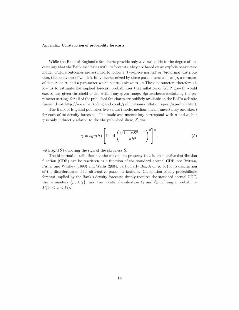
Appendix: Construction of probability forecasts

While the Bank of England’s fan charts provide only a visual guide to the degree of un-

certainty that the Bank associates with its forecasts, they are based on an explicit parametric

model. Future outcomes are assumed to follow a ‘two-piece normal’ or ‘bi-normal’ distribu-

tion, the behaviour of which is fully characterized by three parameters: a mean µ, a measure

of dispersion σ, and a parameter which controls skewness, γ.These parameters therefore al-

low us to estimate the implied forecast probabilities that inflation or GDP growth would

exceed any given threshold or fall within any given range. Spreadsheets containing the pa-

rameter settings for all of the published fan charts are publicly available on the BoE’s web site

(presently at http://www.bankofengland.co.uk/publications/inflationreport/irprobab.htm).

The Bank of England publishes five values (mode, median, mean, uncertainty and skew)

for each of its density forecasts. The mode and uncertainty correspond with µ and σ, but

γ is only indirectly related to the the published skew, S, via

γ = sgn(S)

1− 4

(√1 + πS2 − 1

πS2

)2 1

2

, (5)

with sgn(S) denoting the sign of the skewness S.The bi-normal distribution has the convenient property that its cumulative distribution

function (CDF) can be rewritten as a function of the standard normal CDF; see Brittan,

Fisher and Whitley (1998) and Wallis (2004, particularly Box A on p. 66) for a description

of the distribution and its alternative parameterizations. Calculation of any probabilistic

forecast implied by the Bank’s density forecasts simply requires the standard normal CDF,

the parameters {µ, σ, γ} , and the points of evaluation `1 and `2 defining a probability

P (`1 < x < `2).

14

Notes to Table and Figures

Table 1

Table 1 reports sample estimates of quantities introduced in the text, pertaining to

forecasts for the indicator variable which equals one when either average CPI inflation or

GDP growth exceeds the indicated annual threshold rate over the indicated forecast horizon,

and zero otherwise. MSFE denotes the mean squared forecast error, and ‘MS calibration’

is the sample estimate of the mean squared calibration error, (2). The scaled resolution is

the estimate of the quantity given by equation (3).

Figure 1

Left and middle panels show probability forecasts; ‘+’ represents cases of eventual out-

come below threshold or within bands, circles are cases of outcome above threshold or outside

bands. In right-hand panels each column represents one bin, 0–0.1, 0.1–0.2, ... 0.9–1.0, and

each row one horizon, 0-8. Each square represents, via colour, the height of a histogram

corresponding with the horizon and bin. Ideally, the probability integral transforms would

yield a U(0,1) sequence, so that each row would show uniform values equal to 0.1.

Figure 2

In each panel, lines of the same colour denote the same horizon; for each horizon, the

solid line represents the empirical CDF of probability forecasts for cases in which the event

of interest did occur (e.g., inflation within bands) and the broken line represents cases in

which the event of interest did not occur.

Figure 3

Each panel plots scaled values of mean squared forecast error, -1× calibration error, and

resolution.

15

Table 1: Calibration and resolution of forecastsGDP growth: preliminary release data

Horizon: 0 1 2 3 4 5 6 7 8

Outcome Variance: 0.245 0.243 0.241 0.238 0.240 0.242 0.243 0.245 0.243

MSFE: 0.122 0.158 0.172 0.195 0.217 0.240 0.243 0.263 0.266

Resolution: 0.122 0.084 0.065 0.061 0.049 0.020 0.006 0.007 0.014

MS calibration: 0.002 0.006 0.008 0.019 0.027 0.027 0.015 0.034 0.052

Scaled resolution ∈ [0, 1]: 0.500 0.347 0.268 0.255 0.205 0.081 0.026 0.028 0.056

Calibration p-value 0.747 0.755 0.679 0.561 0.535 0.434 0.554 0.090 0.103

Resolution p-value 0.000 0.000 0.000 0.001 0.033 0.095 0.331 0.904 0.940

GDP growth: 2010Q1 vintage data

Horizon: 0 1 2 3 4 5 6 7 8


MSFE: 0.275 0.292 0.298 0.310 0.281 0.270 0.262 0.264 0.278

Resolution: 0.031 0.021 0.018 0.011 0.016 0.003 0.001 0.006 0.011

MS calibration: 0.065 0.067 0.072 0.070 0.048 0.025 0.015 0.024 0.044




Inflation: target threshold

Horizon: 0 1 2 3 4 5 6 7 8


MSFE: 0.064 0.131 0.171 0.228 0.285 0.291 0.279 0.260 0.267

Resolution: 0.195 0.121 0.080 0.032 0.008 0.008 0.011 0.001 0.003

MS calibration: 0.011 0.006 0.008 0.015 0.047 0.053 0.042 0.010 0.014




Inflation: target band

Horizon: 0 1 2 3 4 5 6 7 8


MSFE: 0.024 0.023 0.058 0.086 0.095 0.093 0.096 0.103 0.116

Resolution: 0.057 0.062 0.042 0.011 0.001 0.001 0.000 0.001 0.002

MS calibration: 0.005 0.008 0.022 0.021 0.016 0.012 0.009 0.013 0.024




16

Figure1

Imp

lied

pro

bab

ilit

yfo

reca

sts

and

pro

bab

ilit

yin

tegr

altr

ansf

orm

s

(i)

GD

Pgr

owth

vs.

thre

shol

d:

2010

Q1

dat

a(l

eft)

;p

reli

min

ary

dat

a(m

idd

le);

PIT

(rig

ht)

Prob

abilit

y

ForecastHorizon

00.2

0.40.6

0.81

02468

0.30

0.26

0.22

0.18

0.14

0.10

0.06

0.02

Figure

2BGD

PFore

cast

Outco

mes

Marke

tInter

estR

ates

(ii)

Infl

atio

nvs.

thre

shol

d:

infl

atio

nw

ith

inb

and

s(l

eft)

orb

elow

targ

et(m

idd

le);

PIT

(rig

ht)

Prob

abilit

y

ForecastHorizon

00.2

0.40.6

0.81

02468

0.18

0.14

0.10

0.06

0.02

Figure

1BInf

lation

Forec

astO

utcom

esMa

rketIn

teres

tRate

s

17

Figure2

Em

pir

ical

CD

F’s

ofim

pli

edp

rob

abil

ity

fore

cast

sfr

omfa

nch

arts

(i)

GD

Pgro

wth

vs.

thre

shol

d;

mar

ket

inte

rest

rate

s,20

10Q

1(l

eft)

and

pre

lim

inar

y(r

ight)

dat

a

(ii)

Infl

ati

on

vs.

thre

shol

d:

mar

ket

inte

rest

rate

s,ca

ses

ofin

flat

ion

wit

hin

ban

ds

(lef

t)an

db

elow

targ

et(r

ight)

18

Figure3

Dec

omp

osit

ion

ofp

rob

abil

ity

fore

cast

MS

E

(i)

GD

Pgr

owth

vs.

thre

shol

d;

mar

ket

inte

rest

rate

s,20

10Q

1(l

eft)

and

pre

lim

inar

y(r

ight)

dat

a

(ii)

Infl

atio

nvs.

thre

shold

:m

arke

tin

tere

stra

tes,

case

sof

infl

atio

nw

ith

inb

and

s(l

eft)

an

db

elow

targ

et(r

ight)

19

assessing gdp and in ation probability forecasts derived

Documents