assessing deterioration of pretimed, actuated- …
TRANSCRIPT
ASSESSING DETERIORATION OF PRETIMED, ACTUATED-
COORDINATED, AND SCOOT CONTROL REGIMES
IN SIMULATION ENVIRONMENT
by
Aleksandar Stevanovic
A dissertation submitted to the faculty of The University of Utah
in partial fulfillment of the requirements for the degree of
Doctor of Philosophy
in
Civil Engineering
Department of Civil and Environmental Engineering
The University of Utah
May 2006

Copyright Aleksandar Stevanovic 2006
All Rights Reserved

THE UNIVERSITY OF UTAH GRADUATE SCHOOL
SUPERVISORY COMMITTEE APPROVAL
of a thesis submitted by
Aleksandar Stevanovic
This thesis has been read by each member of the following supervisory committee and by majority vote has been found to be satisfactory.
_____________________ ___________________________________________
Chair: Peter T. Martin
_____________________ ___________________________________________
Lawrence D. Reaveley
_____________________ ___________________________________________
Pedro Romero
_____________________ ___________________________________________ Philip Emmi
_____________________ ___________________________________________
Larry Head

THE UNIVERSITY OF UTAH GRADUATE SCHOOL
FINAL READING APPROVAL
To the Graduate Council of the University of Utah:
I have read the thesis of Aleksandar Stevanovic in its final form and have found that (1) its format, citations, and bibliographic style are consistent and acceptable; (2) its illustrative materials including figures, tables, and charts are in place; and (3) the final manuscript is satisfactory to the supervisory committee and is ready for submission to The Graduate School.
_____________________ _____________________________________________ Date Peter T. Martin
Chair: Supervisory Committee
Approved for the Major Department
______________________________________________
Lawrence D. Reaveley Chair/Dean
Approved for the Graduate Council
______________________________________________
David S. Chapman Dean of The Graduate School

ABSTRACT
Regular updating of traffic signal timing plans is very important for successful
traffic control. However, many jurisdictions fail to update signal timings because it is
labor intensive and costly. Without updating, signal timings become obsolete as
traffic volumes change. Adaptive traffic control is sometimes perceived as a way to
avoid retiming traffic signals. There are no findings that support this belief.
This research investigates the deterioration of pretimed, actuated-coordinated,
and SCOOT traffic control regimes through the use of microsimulation. Deterioration
of actuated-coordinated and SCOOT adaptive controls have not been investigated
before. Previous attempts to investigate the deterioration of pretimed control did not
use microsimulation. Two major objectives of the study were to develop a
methodology to assess the deterioration of the traffic control regimes through
microsimulation and to evaluate the deterioration of the traffic control regimes with
respect to modeled changes in traffic demand and distribution.
The experimental nine-node grid network is used as a test bed to model
deterministic and stochastic traffic demand and distribution changes in link flows.
Traffic signal plans developed for the base traffic conditions serve as the non-
optimized plans for all other conditions. Optimized plans are developed for each
scenario of changed traffic flows using macroscopic optimization tools.
The results show that all traffic control regimes deteriorate. The results for
pretimed and actuated controls show that there is a benefit of up to 3% for up to 5%

v
of uniform growth in traffic demand for networks with unchanged traffic
distributions. When stochastic variations of traffic demand and distribution are
introduced, the benefits rise to an average of 35% for pretimed control and 27% for
actuated control. Assessment of SCOOT ageing shows that SCOOT performance
highly fluctuates with changes in traffic flows. The SCOOT control performs worse
than optimized pretimed control for most of the scenarios. Had the SCOOT control
been replaced by optimized pretimed plans, benefits of 11 to 16% could be achieved.
The roots of SCOOT ageing have been found in its inability to accurately model
traffic at the intersection approaches for changed traffic flows.

CONTENTS
ABSTRACT................................................................................................................. iv
CONTENTS................................................................................................................. vi
LIST OF FIGURES ................................................................................................... viii
LIST OF TABLES ....................................................................................................... xi
ACRONYMS.............................................................................................................. xii
1. INTRODUCTION .................................................................................................. 1
1.1 Traffic Congestion and Traffic Control .................................................... 1 1.2 Signal Timing Parameters ......................................................................... 3 1.3 Problem Definition.................................................................................... 6 1.4 Research Goal and Objectives .................................................................. 9 1.5 Dissertation Organization ....................................................................... 10
2. LITERATURE REVIEW ..................................................................................... 13
2.1 Traffic Control Systems .......................................................................... 13 2.2 Review of the Studies on Ageing of Traffic Signal Timing Plans ......... 34 2.3 Summary of Literature Review............................................................... 39
3. RESEARCH METHODOLOGY.......................................................................... 41
3.1 The Concept of Ageing of Traffic Control Systems ............................... 41 3.2 Design of the Simulation Experiments ................................................... 55 3.3 Selection of Proper Tools for Assessing the Ageing of Traffic Control. 59 3.4 Major Modeling Process ......................................................................... 90 3.5 Preparing VISSIM-SCOOT Simulations ................................................ 93 3.6 Summary of Research Methodology .................................................... 104
4. RESULTS ........................................................................................................... 106
4.1 Justification of the Adopted Approach for Measuring Ageing............. 106 4.2 Reliability of Bell’s Ageing Measure ................................................... 107 4.3 Ageing of Pretimed and Actuated Traffic Controls .............................. 111 4.4 Ageing of the SCOOT Adaptive Control Regime ................................ 125 4.5 Summary of Results.............................................................................. 135
5. DISCUSSION..................................................................................................... 138
5.1 Methodology for Assessing the Ageing of Traffic Control Regimes ... 138 5.2 Reliability of the Ageing Measure for Changed Traffic Flows ............ 140 5.3 Ageing of Pretimed and Actuated Traffic Control Regimes ................ 141 5.4 Ageing of the SCOOT Control Regime ................................................ 147 5.5 Summary of Discussion........................................................................ 159

vii
6. CONCLUSIONS................................................................................................. 163
6.1 Conclusions ........................................................................................... 163 6.2 Summary of Conclusions ...................................................................... 167 6.3 Future Research..................................................................................... 167
APPENDIX: CORRELATIONS BETWEEN SCOOT AND VISSIM QUEUES ... 170
REFERENCES ......................................................................................................... 183

LIST OF FIGURES
2.1 – Pretimed Signal Timing Plans for Two Adjacent Intersections ......................... 17
2.2 – Actuated Signal Timing Plan for an Intersection............................................... 20
2.3 – SCOOT Adaptive Timing Parameters for an Intersection................................. 21
2.4 – SCOOT Predictions of Downstream Flow ........................................................ 27
3.1 - Impact of the Traffic Changes on the Nonadaptive Traffic Controls ................. 47
3.2 – Ageing of the Traffic Control Regimes with Change in Traffic Flow.............. 50
3.3 - Test Bed Network with Base Traffic Flows (Synchro 6) ................................... 56
3.4 - Method to Assess Reliability of Timing Plans in Simulation Tools .................. 68
3.5 - PI and CL vs. Network Growth for Synchro and Transyt-7F ............................ 73
3.6 - Total Delay vs. Network Growth for Direct CORSIM Optimization ................ 73
3.7 - PI and CL vs. Network Growth for VISSIM and Synchro................................. 74
3.8 – PI and CL vs. Network Growth for VISSIM and Transyt-7F............................ 74
3.9 - PI and CL vs. Network Growth for SimTraffic and Synchro............................. 75
3.10 - PI and CL vs. Network Growth for SimTraffic and Transyt-7F ..................... 75
3.11 - PI and CL vs. Network Growth for Corsim and Synchro ................................ 76
3.12 - PI and CL vs. Network Growth for Corsim and Transyt-7F ............................ 76
3.13 - PI and CL vs. TM Change for Synchro and Transyt-7F .................................. 79
3.14 - Total Delay vs. TM Change for Direct CORSIM Optimization ...................... 79
3.15 - PI and CL vs. TM Change for VISSIM and Synchro....................................... 80
3.16 - PI and CL vs. TM Change for VISSIM and Transyt-7F .................................. 80

ix
3.17 - PI and CL vs. TM Change for SimTraffic and Synchro................................... 81
3.18 - PI and CL vs. TM Change for SimTraffic and Transyt-7F ............................. 81
3.19 - PI and CL vs. TM Change for CORSIM and Synchro ..................................... 82
3.20 - PI and CL vs. TM Change for CORSIM and Transyt-7F ................................ 82
3.21 – Modeling Process for Evaluating Ageing of Traffic Control Regimes ........... 91
3.22 - Internal Structure of VISSIM Simulation Software ......................................... 98
3.23 – VISSIM-SCOOT Simulation Environment .................................................. 100
3.24 – Queue Formation in SCOOT and VISSIM.................................................... 102
3.25 – Correlation between Traffic Queues in SCOOT and VISSIM ...................... 104
4.1 - Modeled Impact of the Uniform Increase in Traffic Demand on PI ................ 107
4.2 - Benefits of Updating vs CF for Decreased Traffic Demand ............................ 108
4.3 - Benefits of Updating vs CF for Increased Traffic Demand .............................. 108
4.4 - Benefits of Updating vs CF for Decreased Turning Movements ..................... 109
4.5 - Benefits of Updating vs CF for Increased Turning Movements ...................... 109
4.6 - Benefits of Updating Timings vs Average Change in Traffic Demand ........... 111
4.7 – PI vs Total Network Growth for Pretimed Traffic Control ............................. 112
4.8 - PI vs Change in Turning Movements for Pretimed Traffic Control................. 113
4.9 - PI vs Total Network Growth for Actuated Traffic Control.............................. 114
4.10 - PI vs Change in Turning Movements for Actuated Traffic Control............... 114
4.11 - Benefits of Updating Timings vs Decrease in Traffic Demand ..................... 121
4.12 - Benefits of Updating Timings vs Increase in Traffic Demand...................... 122
4.13 - Benefits of Updating Timings vs Decrease in Turning Movements ............. 122
4.14 - Benefits of Updating Timings vs Increase in Turning Movements............... 123

x
4.15 - Benefits of Updating Timings vs Change in Traffic Demand ........................ 124
4.16 – PI vs Traffic Growth for SCOOT and Pretimed Traffic Control................... 126
4.17 – PI vs Turning Movements for SCOOT and Pretimed Controls ..................... 132
5.1 – Accuracy of SCOOT Traffic Model vs Traffic Demand ................................. 154
LIST OF TABLES
3.1 – Changes in Traffic Flows and Associated Terms .............................................. 43
3.2 – Calibration of VISSIM Saturation Flow Coefficients ....................................... 96
4.1 – Testing for Pretimed SimTraffic Control – Traffic Demand ........................... 117
4.2 – Testing for Pretimed SimTraffic Control – Traffic Distribution ..................... 118
4.3 – Testing for Actuated SimTraffic Control – Traffic Demand ........................... 119
4.4 – Testing for Actuated SimTraffic Control – Traffic Distribution ..................... 120
4.5 – Testing for Pretimed VISSIM Control – Traffic Demand ............................... 126
4.6 – Testing for SCOOT and Pretimed Control – Traffic Demand......................... 129
4.7 – Testing Ageing of SCOOT Control – Traffic Demand ................................... 132
4.8 – Testing for Pretimed VISSIM Control – Traffic Distribution ......................... 133
4.9 – Testing for SCOOT and Pretimed Control – Traffic Distribution................... 134
4.10 – Testing Ageing for SCOOT – Traffic Distribution........................................ 135
4.11 – Overall SCOOT Performance ........................................................................ 136

ACRONYMS
ATCS Adaptive Traffic Control System
CF Changed Flows
CFP Cyclic Flow Profile
CL Cycle Length
CORSIM CORridor SIMulation
DDE Dynamic Data Exchange
DLL Dynamic Link Library
ELAG End LAG
FHWA Federal HighWay Administration
GA Genetic Algorithms
HCM Highway Capacity Manual
HCS Highway Capacity Software
ITE Institute of Transportation Engineers
JNYT JourNeY Time
LOS Level Of Service
MOE Measures Of Effectiveness
MC3 Managing Congestion, Communications, and Control
NEMA National Electrical Manufacturer Association
NO NonOptimized
NPNT New Plan New Traffic

xiii
OP OPtimized
OPAC Optimized Policies for Adaptive Control
OPNT Old Plan New Traffic
PASSER Progression Analysis and Signal System Evaluation Routine
PI Performance Index
QCMQ Clear time for Maximum Queue
PRIMAVERA PRIority MAnagement for Vehicle efficiency, Environment
Road safety on Arterials
RHODES Real-Time Hierarchical Optimized Distributed and Effective
System
SCATS Sydney Coordinated Adaptive Traffic System
SCJ Signal Control Junction
SCOOT Split Cycle Offset Optimization Technique
SIDRA Signalized Intersection Design and Research Aid
SLAG Start LAG
SOAP Signal Operations Analysis Package
SSD Sum of Squared Differences
STOC SaTuration Occupancy
TCP/IP Transmission Control Protocol / Internet Protocol
TM Turning Movement
TOD Time Of Day
TRANSYT TRAffic Network StudY Tool
TRL Traffic Research Laboratory

xiv
UDOT Utah Department Of Transportation
UTDF Universal Traffic Data Format
UTL Utah Traffic Lab
UTCS Urban Traffic Control System
VAP Vehicle Actuated Programming
V/C Volume/Capacity
VISSIM Verkehr In Stadten SIMulation (Traffic in Towns Simulation)

CHAPTER 1
INTRODUCTION
This chapter addresses the essential background of traffic control systems and
the importance of their maintenance. Signal timing parameters are discussed as one of
the key factors for updating traffic control systems. Then, after a basic literature
review of the most important studies that have been done on the topic, the research
problem is defined. The research goal and objectives are stated in the next part of the
chapter. The final part of the chapter provides an overview to guide readers through
the remainder of the dissertation.
1.1 Traffic Congestion and Traffic Control
The growth in urban traffic congestion has been recognized as a serious
problem in all large metropolitan areas in the country, with significant effects on the
economy, travel behavior and land use, as well as a cause of discomfort for millions
of motorists.
Solutions to the congestion problems are neither simple nor unique. The
traditional approach of simply adding more capacity is often not possible or desirable.
Therefore, improvements are often sought that increase the efficiency of the existing
systems. One of the most important tools to alleviate urban congestion is traffic
control. Maintenance of traffic control systems is as important as their optimizing
methods and initial design.

2
The first traffic signals were installed in the beginning of the 20th century. Their
main objective was to prevent accidents by alternately assigning the right of way. Not
much attention was given to other objectives that are relevant today, such as
minimizing traffic delay and fuel consumption. Over time, however, as traffic
volumes have increased, the objective has broadened to include maximizing the
capacity of the roadway system and improving traffic flow.
The Federal Highway Administration (FHWA) (1995) has reported that there
are more than 300,000 traffic signals in North America. The same study estimated
that two-thirds of all miles driven each year occur on roadways controlled by traffic
signals. Despite their important role in traffic management, after traffic signals are
installed, the timing settings are often not given enough attention. Further, more than
half of the signals in North America are in need of repair (or replacement) of the
traffic signal hardware, or in need of upgrade of the timing plans and traffic control
software (FHWA 1995).
Making improvements to traffic signals can be one of the most cost-effective
tools to increase mobility on arterials. A few simple, low-cost adjustments to a traffic
signal system can often significantly improve traffic flow. In many cases, traffic
signal equipment can be updated. This allows for greater flexibility of timing plans,
including coordination with other nearby signals for progression. In some cases,
existing equipment may be adequate; however, due to changing traffic patterns,
timing plan improvements may be needed to accommodate current traffic flows more
efficiently.
3
Much of the delay experienced by motorists during the day occurs as they wait
for the light to turn green at signalized intersections. Delays can be reduced, however,
by optimizing signal timings. Although more than half of the signalized intersections
in the United States would benefit from equipment upgrades, nearly 1.5 % of the
intersections would benefit from signal timing adjustments alone - without any
hardware changes (FHWA 1995).
Highway agencies are supposed to regularly monitor traffic at intersections and
then update their traffic control strategies, including signal timing plans, to ensure
that a signal system is working properly so that traffic is flowing efficiently and
safely. Unfortunately, this is often not the case (FHWA 2002). Many jurisdictions fail
to update timing control strategies because it is labor intensive and costly. As a result,
the original traffic signal plan for an intersection often continues operating long after
changing traffic volumes have made it outdated.
1.2 Signal Timing Parameters
Federal Highway Administration defines fundamental signal timing variables
as follows (FHWA 1996):
• Cycle Length - the time required to complete one sequence of signal intervals
(phases).
• Phase – the portion of signal cycle allocated to any single combination of one
or more traffic movements simultaneously receiving right-of-way during one
or more intervals.

4
• Interval – a discrete portion of the signal cyc le during which the signal
indications (pedestrian or vehicle) remain unchanged.
• Split – the percentage of a cycle length allocated to each of the various phases
in a signal cycle.
• Offset – the time difference between the start of the green indication at one
intersection as related to the system time reference point.
According to the same handbook (FHWA 1996) cycle length, split and offset are the
three fundamental signal timing variables (also called signal timing parameters). As a
group they are often referred to as ‘signal timings’. The following sentences further
clarify these concepts.
Traffic control and coordination is achieved by applying proper phases, splits,
cycle times, and offsets. The offset is the difference in time between when one
approach (e.g., northbound) on one signal gives green and the time when an adjacent
signal (e.g., also northbound) gives green. The offset is often related to the time it
takes a vehicle to travel between the signals. Coordination is what results from
properly tuned offset values along a corridor.
The cycle time is time from the beginning of green, through amber and red to
the beginning of green on a single signal phase. It is generally more straightforward
to maintain coordination when cycle lengths are equal between adjacent signals. The
split is the proportion of time allotted to each approach (i.e., 20% for the North and
South legs and 80% for the East and West legs).
The three basic types of traffic controls are pretimed control, actuated control,
and adaptive control. These three types represent different approaches to the problem

5
of keeping traffic control up-to-date with changes in traffic conditions. More about
each type will be presented in later chapters. However, all of these traffic control
types have one thing in common: each requires an input to the controller consisting of
initial control settings for the traffic signal timings. Range and depth to which the
traffic control settings (a.k.a. signal timings) are specified in initial timing design
differ significantly among various traffic control types. Hence, the pretimed traffic
control requires that all basic parameters (cycle length, phase splits, intergreen
intervals, and offset) are predetermined. Once these settings are entered, they remain
constant until the next retiming project, which could be years away. The other types
of control (actuated and adaptive) are responsive traffic controls. They respond to
various changes in traffic conditions. While actuated traffic control responds mostly
to changes in traffic distribution (by allocating appropriate amounts of green time to
each traffic movement), adaptive control responds both to changes in traffic demand
and traffic distribution. These control types usually require only broader limits within
which these parameters may vary based on the online variations of traffic conditions.
The initial design for actuated traffic control requires defining parameters, such as
cycle length, offset, minimum green times, maximum green times, passage times,
minimum gaps, etc. An Adaptive Traffic Control System (ATCS) requires either an
extensive library of signal timing parameters or a range within which the system itself
calculates the parameters, depending on the adaptive method used.
It is well known among signal timing practitioners that pretimed traffic control
needs regular updates of the signal timing parameters to cope with changed traffic
conditions (Tarnoff and Ordonez 2004, Sunkari 2004). The other two types of traffic

6
control are known to be effective in coping with changes in traffic demand and/or
traffic distribution. However, the extent and consistency of their effectiveness has not
yet been thoroughly investigated.
Actuated traffic control is generally perceived to need regular updates for some
of the signal timing parameters (cycle length and offsets). However, little is known
about the extensiveness of deterioration of this control type when compared with
pretimed traffic control. On the other hand, most traffic signal practitioners believe
that ATCS do not require any updates. Unlike pretimed and actuated control systems,
which usually change the signal timing plans based on Time-Of-Day (TOD) traffic
patterns prepared off- line, ATCS account for changes in traffic demand (at an
intersection approach). For this reason it is generally believed (and often advertised
by ATCS vendors) that the ATCS do not deteriorate over time (TRL 2003, TYCO
2003). In other words, it is believed that once the signal timings are initially entered
and calibrated, the systems take care of their adjustment regardless of the changes in
traffic. The literature does not provide enough evidence to support or reject these
beliefs. There is no study or article describing the behavior of ATCS when traffic
conditions are changed over the long term. Therefore, either the ageing of ATCS has
not been investigated enough, or the results of such investigations have not been
published.
1.3 Problem Definition
In the last 20 years, investigation of the benefits and disbenefits of the
deterioration of traffic control systems has not drawn a lot of attention from traffic

7
researchers. The first significant attempts to overcome the obsolescence of pretimed
signals were made in the 1970s. The pretimed TOD traffic signals’ inability to
respond to traffic fluctuations led to the development of several ATCS (Hunt et al.
1981, Lowrie 1982, Gartner 1983) in the late 1970s and the early 1980s. The benefits
of ATCS over pretimed signal systems were perceived and quantified right after the
first ATCS were implemented. These benefits were well documented in several
studies (Robertson and Hunt 1982, Luk et al. 1982, 1983, Robertson 1987). However,
most of these benefits are associated with diurnal or weekly changes of traffic
demand and distribution. They are not associated with any long-term changes in
traffic conditions.
The benefits of updating the pretimed control systems (or disbenefits of not
updating, which is an equivalent measure of deterioration) were not investigated until
1986. The key research was conducted by Bell (1985), comprehensively quantifying
the disbenefits of not updating the aged pretimed traffic signal systems. The results
showed that the disbenefits for grid networks were around 3.8% per year, with up to
four years elapsed time between updates. Much later, two additional studies estimated
the disbenefits of traffic signal ageing. The FHWA Primer (FHWA 1995) reports that
improvement of coordinated traffic signal timing plans reduces travel times by 12%
on average. A study from the Institute of Transportation Engineers (ITE) (Sunkari
2004) illustrates that user costs increase substantially if timing plans are not updated
at least every three years. These two studies, however, do not provide details for the
assumptions and methodology used to estimate the costs of not updating timing plans.
So, the Bell and Bretherton study remains the major research. It is frequently cited in

8
reference to the obsoleteness of pretimed signal systems (Luyanda et al. 2003, Fehon
2004). More on the shortcomings of previous research on the deterioration of
pretimed control is given in the Chapter 2 of the dissertation.
There is no investigation on deterioration of performance due to change in
traffic conditions for the other two major types of traffic controls (actuated and
adaptive). There are two major reasons for the lack of research in deterioration of
adaptive control. First, the ATCS are expensive and, therefore, not easily available to
traffic researchers. As such, the systems are usually installed and used by government
agencies for traffic control purposes only. Second, the ATCS developers and vendors
which are able to investigate their systems might be hesitant to publish findings
revealing potential shortcomings of the systems. However, even more surprising is
that there is no published research quantifying the deterioration of actuated traffic
control – the form of control that is currently used at most intersections in the USA.
The purpose of this study is to quantify the level of deterioration for actuated
and adaptive controls and to give an update on the deterioration of pretimed control.
The first contribution of this dissertation to the body of knowledge comes from the
fact that no previous research has assessed the deterioration of actuated and adaptive
traffic controls. The second contribution of this study is the development of the
methodology to quantify this deterioration for adaptive traffic control. More on this
subject is provided in the Chapter 3 of the dissertation.
Pretimed and actuated traffic controls are standard controls that can be found at
most traffic signals throughout the world. Unlike pretimed and actuated controls,
deploying adaptive traffic control means purchasing a license and installing

9
technology, which enables use of real- time detector data to adjust/optimize traffic
flows in the network. Adaptive installations often require even more than that. They
are customized and tailored to satisfy specific requirements considering the
idiosyncrasies of specific road and traffic conditions. More information about various
adaptive controls is given in the Chapter 2 of the dissertation.
SCOOT (Split Cycle Offset Optimization Technique) is selected to be a
representative of adaptive control for this study. There are two reasons for selecting
SCOOT. First, SCOOT is one of the most well-known and widely used adaptive
techniques in the world. Second, the first academic license to use SCOOT was
presented to the University of Utah in Salt Lake City, Utah. By conducting this
research at the Utah Traffic Lab (UTL), the author has the unique opportunity of
using the actual SCOOT control interfaced to the VISSIM traffic simulation software
(Hansen and Martin 1998, Feng and Martin 2002).
The research questions that motivated this study relate unknown impact of
changes in traffic flows on the degradation of the performance of various traffic
control regimes. The first question for each control type is whether the control regime
deteriorates with changes in traffic flows. The second question is whether the
deterioration of each control type is smaller or larger than the deterioration of other
control types.
1.4 Research Goal and Objectives
The goal of the study is to investigate the deterioration of various traffic control
regimes. Three traffic control regimes are selected representing pretimed traffic

10
control, actuated traffic control, and adaptive traffic control. Their performances are
evaluated on the network of urban arterials for various changes in traffic demand and
distribution. The major objectives of the study are:
• Develop methodology to assess deterioration of the traffic control regimes
through microsimulation
• Evaluate deterioration of the traffic control regimes with respect to modeled
changes in traffic demand and distribution
The foundation of this research lies in three major hypotheses. The hypotheses
are based on the case that signal timing parameters are not updated regularly. The
hypotheses are:
1. H0(1) - Pretimed traffic control plans do not deteriorate with changes in
traffic demand and distribution
2. H0(2) - Actuated traffic control plans do not deteriorate with changes in
traffic demand and distribution
3. H0(3) – SCOOT adaptive traffic control does not deteriorate with changes
in traffic demand and distribution
1.5 Dissertation Organization
This dissertation is divided into six chapters. Chapter 1 – Introduction
introduces the reader to the essential background of traffic control systems and the
importance of their maintenance. Signal timing parameters are discussed as one of the
key factors for updating traffic control systems. In the later part of the chapter the

11
research problem was stated and the goal and the objectives of the research were
stated.
Chapter 2 – Literature Review provides a comprehensive overview of the
related research. The literature review concentrates on two topics. The first topic
deals with various types of traffic control used in this study. A short history of traffic
control systems, types of traffic control, and, their most essential features are
presented. Special emphasis is given to the SCOOT system since it is the most
complex and least known control type used in this study.
Chapter 3 – Research Methodology describes the approach to conducting the
research. The first part of the chapter introduces the concept of ageing of traffic
control regimes. A method is proposed to measure the extent of the signal timing
plans’ ageing. The next part of the chapter presents the network and the set of
assumptions used to design simulation experiments. Selection of appropriate tools for
assessing the ageing of signal timing plans follows. This section represents a study
within the main study. It has its own literature review, methodology, results, and
discussion. The next part of the chapter deals with the main modeling process. It
describes modeling experiments for the three types of traffic control and validation of
the SCOOT model. The last part of the chapter summarizes the research methodology
and presents its findings.
Chapter 4 – Results provides the findings of the experiments. The results are
presented in the form of graphs and tables with short discussion of their meanings.
The chapter is divided into four sections. The first part of the chapter presents a
general finding about the methodology used in this study. The second section deals

12
with the reliability of the ageing measure used in Bell’s work. The third part of the
chapter presents the results for ageing of pretimed and actuated-coordinated traffic
control regimes for deterministic and stochastic changes in traffic flows. The final
part of the chapter shows the results of assessing the ageing of SCOOT adaptive
control.
Chapter 5 – Discussion analyzes the results presented in the previous chapter.
First, the general methodology used to assess the ageing of traffic control is
discussed. Next, the ageing measure used by Bell is discussed, along with the reason
for its inability to provide a reliable measure of aged traffic flows. The third part of
this chapter discusses the results of assessed ageing of pretimed and actuated traffic
control regimes. Specific reasons for the particular results are provided. The last part
of the chapter discusses SCOOT performance and the ageing of the SCOOT control.
Chapter 6 – Conclusions provides conclusions of the research and directions for
future research.

CHAPTER 2
LITERATURE REVIEW
This chapter presents the findings of the literature review. A comprehensive
literature search is done and findings are grouped into three subchapters. The first
section reviews the different types of traffic control used in this study. It presents a
short history of traffic control systems, types of traffic control and their most essential
features. Special emphasis is given to the SCOOT system since it is the most complex
and least known control type used in this study. The second part of the chapter
provides a review of a few studies that have investigated the deterioration of traffic
control systems. The final part of the chapter summarizes the literature review.
2.1 Traffic Control Systems
Over the past few decades, traffic signal control systems have evolved along
with technological advancements in electronic, communication, control, and
computer fields. Computers have allowed the development of off- line traffic signal
optimization. One type of optimization philosophy, represented by Traffic Network
Study Tool 7F (TRANSYT 7F) (Robertson 1969) and SYNCHRO (Husch and
Albeck 2003 (I)), models vehicle arrivals at each approach to an intersection and
attempts to minimize delays, stops, and queue lengths. A second type of philosophy
uses bandwidth maximization to determine the number of vehicles that can progress
along a series of signals based on a time-space relationship. Some specific

14
applications of this philosophy are MAXBAND (Little et al. 1981), PASSER-II
(Chang 1988) and REALBAND (Dell'Olmo and Mirchandani 1995). These
optimization techniques are used with historical traffic flows to produce a fixed-time
plan. These plans are typically implemented during times of the day when traffic
flows are distinct, such as during the morning and evening commute hours. Because
these plans are based on historical flows, they require periodic updating. It has been
shown that these plans degrade (deteriorate) by 3-5% per year (Bell and Bretherton
1986). Often, municipalities will update these plans infrequently because of cost
constraints, resulting in an inefficient signal-timing plan.
The FHWA sponsored a research program called the UTCS (Urban Traffic
Control System) in the 1970s as a way to improve performance of traffic signal
systems. The research developed and tested three strategies (or generations) of
adaptive traffic signal control (MacGowan and Fullerton 1979):
Generation 1 (1GC) uses prestored signal timing plans that are calculated off-
line and are based on historical data. These either go into effect at a specific time of
day or by an operator selecting the best-suited plan from an existing library of plans
for the various traffic conditions on that network.
Generation 1.5 (1.5GC) is the same as 1GC, except new timing plans are
generated automatically when traffic conditions warrant them.
Generation 2 (2GC) calculates and implements timing plans based on
surveillance data. This is repeated at 5-minute intervals. To avoid too much change,
the system is not allowed to implement a change at two 5-minute intervals in a row,
or to have varying cycle lengths on signals within a group.

15
Generation 3 (3GC) is similar to 2GC, except it is allowed to change cycle
lengths at 3-5-minute intervals and the cycle length is allowed to vary between
signals as well as during the same control period.
Field tests performed on these control strategies yielded surprising results.
Generation 1 performed the best. Within 1GC, plans selected by an operator
functioned better than the time-of-day plans. Generation 2 had a mix of success and
failure. The average benefit, however, was inferior to 1GC. Generation 3 was
unsuccessful altogether and degraded conditions in almost every case.
Some hypotheses for why the failures occurred are:
• inaccuracies in flow measurement caused 2GC and 3GC to not be able to
respond quickly enough
• inadequate transition logic was used between plans, causing traffic to be
caught in the middle of progression (transients), and
• the benefit of coordination outweighed the benefit of local signal
optimization.
Modern traffic control systems can be divided into three major categories:
pretimed, actuated, and adaptive. Pretimed traffic control and actuated traffic control
are frequently referred to as fixed timing controls.
2.1.1 Pretimed Traffic Control Systems
Pretimed controllers represent traffic control in its most basic form. They
operate on a predetermined and regularly repeated sequence of signal indications. The
pretimed traffic control systems use controllers that require constant cycle time

16
length, split length and split sequence. Signal timing plans are developed off- line and
optimized according to historical traffic flow data. Traffic control systems commonly
have a series of predetermined plans to accommodate variations in traffic volume
during the day, such as peak and off-peak traffic conditions .
Figure 2.1 shows two coordinated intersections with pretimed control and four
phases for traffic movements. Coincidently, these two intersections have the same
splits. In reality, the splits do not have to be equal but if intersections are coordinated
they will always have the same cycle length. Offset between intersections defines
beginning of the coordinated phase at the slave intersection (Phase 4 in Figure 2.1) in
order for traffic to get progression between these two intersections. Progression refers
to the nonstop movement of vehicles along a signalized street system.
Pretimed controllers are best suited for intersections where traffic volumes are
predictable, stable, and fairly constant. Once the timing programs are set, they are
updated to adjust to changes in traffic flow. The frequency of the updating largely
depends on the variation of traffic flow and available resources. Generally, pretimed
controllers are cheaper to purchase, install, and maintain than traffic-actuated
controllers. Their repetitive nature facilitates coordination with adjacent signals, and
they are useful where progression is needed. Properly timed signal systems facilitate
progression.
Many algorithms for developing pretimed signal plans were developed.
Software packages were developed to design isolated- intersection signal times,
including Highway Capacity Software (HCS), Signal Operations Analysis Package

17
I I I I I I I I I I I I I I I I I I I I I I I I I I I I I I I I I I I I I I I I I I I I I I I I I I I I I I I I I I I I I II I I I I I I I I I I I I I I I I I I I I I I I I I I I I I I I I I I I I I I I I I I I I I I I I I I I I I I I I I I I I II I I I I I I I I I I I I I I I I I I I I I I I I I I I I I I I I I I I I I I I I I I I I I I I I I I I I I I I I I I I I II I I I I I I I I I I I I I I I I I I I I I I I I I I I I I I I I I I I I I I I I I I I I I I I I I I I I I I I I I I I I II I I I I I I I I I I I I I I I I I I I I I I I I I I I I I I I I I I I I I I I I I I I I I I I I I I I I I I I I I I I I II I I I I I I I I I I I I I I I I I I I I I I I I I I I I I I I I I I I I I I I I I I I I I I I I I I I I I I I I I I I I II I I I I I I I I I I I I I I I I I I I I I I I I I I I I I I I I I I I I I I I I I I I I I I I I I I I I I I I I I I I I II I I I I I I I I I I I I I I I I I I I I I I I I I I I I I I I I I I I I I I I I I I I I I I I I I I I I I I I I I I I I II I I I I I I I I I I I I I I I I I I I I I I I I I I I I I I I I I I I I I I I I I I I I I I I I I I I I I I I I I I I I II I I I I I I I I I I I I I I I I I I I I I I I I I I I I I I I I I I I I I I I I I I I I I I I I I I I I I I I I I I I I II I I I I I I I I I I I I I I I I I I I I I I I I I I I I I I I I I I I I I I I I I I I I I I I I I I I I I I I I I I I I II I I I I I I I I I I I I I I I I I I I I I I I I I I I I I I I I I I I I I I I I I I I I I I I I I I I I I I I I I I I I II I I I I I I I I I I I I I I I I I I I I I I I I I I I I I I I I I I I I I I I I I I I I I I I I I I I I I I I I I I I I II I I I I I I I I I I I I I I I I I I I I I I I I I I I I I I I I I I I I I I I I I I I I I I I I I I I I I I I I I I I I II I I I I I I I I I I I I I I I I I I I I I I I I I I I I I I I I I I I I I I I I I I I I I I I I I I I I I I I I I I I I II I I I I I I I I I I I I I I I I I I I I I I I I I I I I I I I I I I I I I I I I I I I I I I I I I I I I I I I I I I I I II I I I I I I I I I I I I I I I I I I I I I I I I I I I I I I I I I I I I I I I I I I I I I I I I I I I I I I I I I I I I II I I I I I I I I I I I I I I I I I I I I I I I I I I I I I I I I I I I I I I I I I I I I I I I I I I I I I I I I I I I I II I I I I I I I I I I I I I I I I I I I I I I I I I I I I I I I I I I I I I I I I I I I I I I I I I I I I I I I I I I I I I/ / / / / / / / / / / / / / / / / / / / / / / / / / / / / / / / / / / / / / / / / / / / / / / / / / / / / / / / / / / / / // / / / / / / / / / / / / / / / / / / / / / / / / / / / / / / / / / / / / / / / / / / / / / / / / / / / / / / / / / / / / // / / / / / / / / / / / / / / / / / / / / / / / / / / / / / / / / / / / / / / / / / / / / / / / / / / / / / / / / / / / / /. . . . . . . . . . . . . . . . . . . . . . . . . . . . . . . . . . . . . . . . . . . . . . . . . . . . . . . . . . . . . .I I I I I I I I I I I I I I I I I I I I I I I I I I I I I I I I I I I I I I I I I I I I I I I I I I I I I I I I I I I I I II I I I I I I I I I I I I I I I I I I I I I I I I I I I I I I I I I I I I I I I I I I I I I I I I I I I I I I I I I I I I II I I I I I I I I I I I I I I I I I I I I I I I I I I I I I I I I I I I I I I I I I I I I I I I I I I I I I I I I I I I I II I I I I I I I I I I I I I I I I I I I I I I I I I I I I I I I I I I I I I I I I I I I I I I I I I I I I I I I I I I I I II I I I I I I I I I I I I I I I I I I I I I I I I I I I I I I I I I I I I I I I I I I I I I I I I I I I I I I I I I I I I II I I I I I I I I I I I I I I I I I I I I I I I I I I I I I I I I I I I I I I I I I I I I I I I I I I I I I I I I I I I I I/ / / / / / / / / / / / / / / / / / / / / / / / / / / / / / / / / / / / / / / / / / / / / / / / / / / / / / / / / / / / / // / / / / / / / / / / / / / / / / / / / / / / / / / / / / / / / / / / / / / / / / / / / / / / / / / / / / / / / / / / / / // / / / / / / / / / / / / / / / / / / / / / / / / / / / / / / / / / / / / / / / / / / / / / / / / / / / / / / / / / / / / /. . . . . . . . . . . . . . . . . . . . . . . . . . . . . . . . . . . . . . . . . . . . . . . . . . . . . . . . . . . . . .I I I I I I I I I I I I I I I I I I I I I I I I I I I I I I I I I I I I I I I I I I I I I I I I I I I I I I I I I I I I I II I I I I I I I I I I I I I I I I I I I I I I I I I I I I I I I I I I I I I I I I I I I I I I I I I I I I I I I I I I I I II I I I I I I I I I I I I I I I I I I I I I I I I I I I I I I I I I I I I I I I I I I I I I I I I I I I I I I I I I I I I II I I I I I I I I I I I I I I I I I I I I I I I I I I I I I I I I I I I I I I I I I I I I I I I I I I I I I I I I I I I I II I I I I I I I I I I I I I I I I I I I I I I I I I I I I I I I I I I I I I I I I I I I I I I I I I I I I I I I I I I I I II I I I I I I I I I I I I I I I I I I I I I I I I I I I I I I I I I I I I I I I I I I I I I I I I I I I I I I I I I I I I II I I I I I I I I I I I I I I I I I I I I I I I I I I I I I I I I I I I I I I I I I I I I I I I I I I I I I I I I I I I I II I I I I I I I I I I I I I I I I I I I I I I I I I I I I I I I I I I I I I I I I I I I I I I I I I I I I I I I I I I I I II I I I I I I I I I I I I I I I I I I I I I I I I I I I I I I I I I I I I I I I I I I I I I I I I I I I I I I I I I I I I II I I I I I I I I I I I I I I I I I I I I I I I I I I I I I I I I I I I I I I I I I I I I I I I I I I I I I I I I I I I I II I I I I I I I I I I I I I I I I I I I I I I I I I I I I I I I I I I I I I I I I I I I I I I I I I I I I I I I I I I I I II I I I I I I I I I I I I I I I I I I I I I I I I I I I I I I I I I I I I I I I I I I I I I I I I I I I I I I I I I I I I II I I I I I I I I I I I I I I I I I I I I I I I I I I I I I I I I I I I I I I I I I I I I I I I I I I I I I I I I I I I I II I I I I I I I I I I I I I I I I I I I I I I I I I I I I I I I I I I I I I I I I I I I I I I I I I I I I I I I I I I I I II I I I I I I I I I I I I I I I I I I I I I I I I I I I I I I I I I I I I I I I I I I I I I I I I I I I I I I I I I I I I II I I I I I I I I I I I I I I I I I I I I I I I I I I I I I I I I I I I I I I I I I I I I I I I I I I I I I I I I I I I I II I I I I I I I I I I I I I I I I I I I I I I I I I I I I I I I I I I I I I I I I I I I I I I I I I I I I I I I I I I I I II I I I I I I I I I I I I I I I I I I I I I I I I I I I I I I I I I I I I I I I I I I I I I I I I I I I I I I I I I I I I II I I I I I I I I I I I I I I I I I I I I I I I I I I I I I I I I I I I I I I I I I I I I I I I I I I I I I I I I I I I I I/ / / / / / / / / / / / / / / / / / / / / / / / / / / / / / / / / / / / / / / / / / / / / / / / / / / / / / / / / / / / / // / / / / / / / / / / / / / / / / / / / / / / / / / / / / / / / / / / / / / / / / / / / / / / / / / / / / / / / / / / / / // / / / / / / / / / / / / / / / / / / / / / / / / / / / / / / / / / / / / / / / / / / / / / / / / / / / / / / / / / / / / /. . . . . . . . . . . . . . . . . . . . . . . . . . . . . . . . . . . . . . . . . . . . . . . . . . . . . . . . . . . . . .I I I I I I I I I I I I I I I I I I I I I I I I I I I I I I I I I I I I I I I I I I I I I I I I I I I I I I I I I I I I I II I I I I I I I I I I I I I I I I I I I I I I I I I I I I I I I I I I I I I I I I I I I I I I I I I I I I I I I I I I I I II I I I I I I I I I I I I I I I I I I I I I I I I I I I I I I I I I I I I I I I I I I I I I I I I I I I I I I I I I I I I II I I I I I I I I I I I I I I I I I I I I I I I I I I I I I I I I I I I I I I I I I I I I I I I I I I I I I I I I I I I I II I I I I I I I I I I I I I I I I I I I I I I I I I I I I I I I I I I I I I I I I I I I I I I I I I I I I I I I I I I I I II I I I I I I I I I I I I I I I I I I I I I I I I I I I I I I I I I I I I I I I I I I I I I I I I I I I I I I I I I I I I I/ / / / / / / / / / / / / / / / / / / / / / / / / / / / / / / / / / / / / / / / / / / / / / / / / / / / / / / / / / / / / // / / / / / / / / / / / / / / / / / / / / / / / / / / / / / / / / / / / / / / / / / / / / / / / / / / / / / / / / / / / / // / / / / / / / / / / / / / / / / / / / / / / / / / / / / / / / / / / / / / / / / / / / / / / / / / / / / / / / / / / / / /. . . . . . . . . . . . . . . . . . . . . . . . . . . . . . . . . . . . . . . . . . . . . . . . . . . . . . . . . . . . . .
Phase 2
Phase 3
Phase 4
Phase 1
Cyc
le L
engt
h
Spl
it2
Spl
it3
Spl
it4
Spl
it1
MASTER INTERSECTION
I I I I I I I I I I I I I I I I I I I I I I I I I I I I I I I I I I I I I I I I I I I I I I I I I I I I I I I I I I I I I II I I I I I I I I I I I I I I I I I I I I I I I I I I I I I I I I I I I I I I I I I I I I I I I I I I I I I I I I I I I I II I I I I I I I I I I I I I I I I I I I I I I I I I I I I I I I I I I I I I I I I I I I I I I I I I I I I I I I I I I I I II I I I I I I I I I I I I I I I I I I I I I I I I I I I I I I I I I I I I I I I I I I I I I I I I I I I I I I I I I I I I II I I I I I I I I I I I I I I I I I I I I I I I I I I I I I I I I I I I I I I I I I I I I I I I I I I I I I I I I I I I I II I I I I I I I I I I I I I I I I I I I I I I I I I I I I I I I I I I I I I I I I I I I I I I I I I I I I I I I I I I I I II I I I I I I I I I I I I I I I I I I I I I I I I I I I I I I I I I I I I I I I I I I I I I I I I I I I I I I I I I I I I II I I I I I I I I I I I I I I I I I I I I I I I I I I I I I I I I I I I I I I I I I I I I I I I I I I I I I I I I I I I I II I I I I I I I I I I I I I I I I I I I I I I I I I I I I I I I I I I I I I I I I I I I I I I I I I I I I I I I I I I I I II I I I I I I I I I I I I I I I I I I I I I I I I I I I I I I I I I I I I I I I I I I I I I I I I I I I I I I I I I I I I II I I I I I I I I I I I I I I I I I I I I I I I I I I I I I I I I I I I I I I I I I I I I I I I I I I I I I I I I I I I I II I I I I I I I I I I I I I I I I I I I I I I I I I I I I I I I I I I I I I I I I I I I I I I I I I I I I I I I I I I I I II I I I I I I I I I I I I I I I I I I I I I I I I I I I I I I I I I I I I I I I I I I I I I I I I I I I I I I I I I I I I II I I I I I I I I I I I I I I I I I I I I I I I I I I I I I I I I I I I I I I I I I I I I I I I I I I I I I I I I I I I I II I I I I I I I I I I I I I I I I I I I I I I I I I I I I I I I I I I I I I I I I I I I I I I I I I I I I I I I I I I I I II I I I I I I I I I I I I I I I I I I I I I I I I I I I I I I I I I I I I I I I I I I I I I I I I I I I I I I I I I I I I II I I I I I I I I I I I I I I I I I I I I I I I I I I I I I I I I I I I I I I I I I I I I I I I I I I I I I I I I I I I I II I I I I I I I I I I I I I I I I I I I I I I I I I I I I I I I I I I I I I I I I I I I I I I I I I I I I I I I I I I I I II I I I I I I I I I I I I I I I I I I I I I I I I I I I I I I I I I I I I I I I I I I I I I I I I I I I I I I I I I I I I I/ / / / / / / / / / / / / / / / / / / / / / / / / / / / / / / / / / / / / / / / / / / / / / / / / / / / / / / / / / / / / // / / / / / / / / / / / / / / / / / / / / / / / / / / / / / / / / / / / / / / / / / / / / / / / / / / / / / / / / / / / / // / / / / / / / / / / / / / / / / / / / / / / / / / / / / / / / / / / / / / / / / / / / / / / / / / / / / / / / / / / / / /. . . . . . . . . . . . . . . . . . . . . . . . . . . . . . . . . . . . . . . . . . . . . . . . . . . . . . . . . . . . . .I I I I I I I I I I I I I I I I I I I I I I I I I I I I I I I I I I I I I I I I I I I I I I I I I I I I I I I I I I I I I II I I I I I I I I I I I I I I I I I I I I I I I I I I I I I I I I I I I I I I I I I I I I I I I I I I I I I I I I I I I I II I I I I I I I I I I I I I I I I I I I I I I I I I I I I I I I I I I I I I I I I I I I I I I I I I I I I I I I I I I I I II I I I I I I I I I I I I I I I I I I I I I I I I I I I I I I I I I I I I I I I I I I I I I I I I I I I I I I I I I I I I II I I I I I I I I I I I I I I I I I I I I I I I I I I I I I I I I I I I I I I I I I I I I I I I I I I I I I I I I I I I I II I I I I I I I I I I I I I I I I I I I I I I I I I I I I I I I I I I I I I I I I I I I I I I I I I I I I I I I I I I I I I/ / / / / / / / / / / / / / / / / / / / / / / / / / / / / / / / / / / / / / / / / / / / / / / / / / / / / / / / / / / / / // / / / / / / / / / / / / / / / / / / / / / / / / / / / / / / / / / / / / / / / / / / / / / / / / / / / / / / / / / / / / // / / / / / / / / / / / / / / / / / / / / / / / / / / / / / / / / / / / / / / / / / / / / / / / / / / / / / / / / / / / / /. . . . . . . . . . . . . . . . . . . . . . . . . . . . . . . . . . . . . . . . . . . . . . . . . . . . . . . . . . . . . .I I I I I I I I I I I I I I I I I I I I I I I I I I I I I I I I I I I I I I I I I I I I I I I I I I I I I I I I I I I I I II I I I I I I I I I I I I I I I I I I I I I I I I I I I I I I I I I I I I I I I I I I I I I I I I I I I I I I I I I I I I II I I I I I I I I I I I I I I I I I I I I I I I I I I I I I I I I I I I I I I I I I I I I I I I I I I I I I I I I I I I I II I I I I I I I I I I I I I I I I I I I I I I I I I I I I I I I I I I I I I I I I I I I I I I I I I I I I I I I I I I I I II I I I I I I I I I I I I I I I I I I I I I I I I I I I I I I I I I I I I I I I I I I I I I I I I I I I I I I I I I I I I II I I I I I I I I I I I I I I I I I I I I I I I I I I I I I I I I I I I I I I I I I I I I I I I I I I I I I I I I I I I I II I I I I I I I I I I I I I I I I I I I I I I I I I I I I I I I I I I I I I I I I I I I I I I I I I I I I I I I I I I I I II I I I I I I I I I I I I I I I I I I I I I I I I I I I I I I I I I I I I I I I I I I I I I I I I I I I I I I I I I I I I II I I I I I I I I I I I I I I I I I I I I I I I I I I I I I I I I I I I I I I I I I I I I I I I I I I I I I I I I I I I I II I I I I I I I I I I I I I I I I I I I I I I I I I I I I I I I I I I I I I I I I I I I I I I I I I I I I I I I I I I I I II I I I I I I I I I I I I I I I I I I I I I I I I I I I I I I I I I I I I I I I I I I I I I I I I I I I I I I I I I I I I II I I I I I I I I I I I I I I I I I I I I I I I I I I I I I I I I I I I I I I I I I I I I I I I I I I I I I I I I I I I I II I I I I I I I I I I I I I I I I I I I I I I I I I I I I I I I I I I I I I I I I I I I I I I I I I I I I I I I I I I I I II I I I I I I I I I I I I I I I I I I I I I I I I I I I I I I I I I I I I I I I I I I I I I I I I I I I I I I I I I I I I II I I I I I I I I I I I I I I I I I I I I I I I I I I I I I I I I I I I I I I I I I I I I I I I I I I I I I I I I I I I I II I I I I I I I I I I I I I I I I I I I I I I I I I I I I I I I I I I I I I I I I I I I I I I I I I I I I I I I I I I I I II I I I I I I I I I I I I I I I I I I I I I I I I I I I I I I I I I I I I I I I I I I I I I I I I I I I I I I I I I I I I II I I I I I I I I I I I I I I I I I I I I I I I I I I I I I I I I I I I I I I I I I I I I I I I I I I I I I I I I I I I I II I I I I I I I I I I I I I I I I I I I I I I I I I I I I I I I I I I I I I I I I I I I I I I I I I I I I I I I I I I I I I/ / / / / / / / / / / / / / / / / / / / / / / / / / / / / / / / / / / / / / / / / / / / / / / / / / / / / / / / / / / / / // / / / / / / / / / / / / / / / / / / / / / / / / / / / / / / / / / / / / / / / / / / / / / / / / / / / / / / / / / / / / // / / / / / / / / / / / / / / / / / / / / / / / / / / / / / / / / / / / / / / / / / / / / / / / / / / / / / / / / / / / / /. . . . . . . . . . . . . . . . . . . . . . . . . . . . . . . . . . . . . . . . . . . . . . . . . . . . . . . . . . . . . .I I I I I I I I I I I I I I I I I I I I I I I I I I I I I I I I I I I I I I I I I I I I I I I I I I I I I I I I I I I I I II I I I I I I I I I I I I I I I I I I I I I I I I I I I I I I I I I I I I I I I I I I I I I I I I I I I I I I I I I I I I II I I I I I I I I I I I I I I I I I I I I I I I I I I I I I I I I I I I I I I I I I I I I I I I I I I I I I I I I I I I I II I I I I I I I I I I I I I I I I I I I I I I I I I I I I I I I I I I I I I I I I I I I I I I I I I I I I I I I I I I I I II I I I I I I I I I I I I I I I I I I I I I I I I I I I I I I I I I I I I I I I I I I I I I I I I I I I I I I I I I I I I II I I I I I I I I I I I I I I I I I I I I I I I I I I I I I I I I I I I I I I I I I I I I I I I I I I I I I I I I I I I I I/ / / / / / / / / / / / / / / / / / / / / / / / / / / / / / / / / / / / / / / / / / / / / / / / / / / / / / / / / / / / / // / / / / / / / / / / / / / / / / / / / / / / / / / / / / / / / / / / / / / / / / / / / / / / / / / / / / / / / / / / / / // / / / / / / / / / / / / / / / / / / / / / / / / / / / / / / / / / / / / / / / / / / / / / / / / / / / / / / / / / / / / /. . . . . . . . . . . . . . . . . . . . . . . . . . . . . . . . . . . . . . . . . . . . . . . . . . . . . . . . . . . . . .
Phase 2
Phase 3
Phase 4
Phase 1
Offs
et
SLAVE INTERSECTION
Figure 2.1 – Pretimed Signal Timing Plans for Two Adjacent Intersections

18
(SOAP) (Courage et al. 1979), SIGNAL94 (Strong Concepts 1995), and Signalized
Intersection Design and Research Aid (SIDRA) (Akcelik and Besley 1998). Some
packages, such as HCS, Progression Analysis and Signal System Evaluation Routine
(PASSER III), MAXBAND, TRANSYT-7F, and SYNCHRO, are for arterial signal
timing design. TRANSYT-7F, SYNCHRO, and PASSER IV can also design signal-
timing plans on networks. A report (Sabra et al. 2000) compared several factors of
these signal-timing packages, including applications, animation, measures of
effectiveness, data input requirements, operating system, and minimum hardware
requirements.
2.1.2 Actuated Traffic Control System
A simple traffic-actuated signal installation consists of four basic components:
detectors, the controller unit, signal heads (the traffic lights), and communications.
Traffic-actuated control systems differ from pretimed control systems. Their signal
indications are not of fixed duration, but rather change in response to variations in the
traffic volumes. Traffic-actuated controllers are typically used where traffic volumes
fluctuate irregularly or where it is necessary to minimize interruptions to traffic flow
on the street carrying the greater volume of traffic.
There are two major types of actuated signal control systems: semi-actuated
and fully-actuated. Semi-actuated systems give green time to minor streets only when
a vehicle is detected. These systems are most appropriate for locations with a low
volume of minor street traffic. Fully-actuated control systems detect vehicles for all
approaches and serve phases as demand on all approaches. Both semi-actuated and

19
fully-actuated signal control systems can be uncoordinated or coordinated. Some
systems can select the best signal- timing plan from a library according to recent ly
measured traffic conditions (called Traffic Responsive Pattern Selection).
This research investigates only coordinated actuated systems. Uncoordinated
actuated control is good only for individual intersections where coordination of green
times at adjacent intersections is not important for progression of vehicles. A grid
network of relatively closely spaced intersections is used for the experiments
conducted in this research. Coordinated actuated traffic control is the only method
that makes sense in the study network, due to the geometric conditions of the
network. Uncoordinated actuated control would not be able to yield performance
comparable to any type of coordinated traffic control.
Actuated signal timing plans are also predesigned by off- line signal timing
design packages, including SOAP, SIGNAL94, TRANSYT-7F, SIDRA, and
SYNCHRO. The cycle time lengths and offsets remain constant. However, actuated
signal control systems can adjust the lengths of phases between minimum and
maximum thresholds in response to vehicle actuations, or they can skip phases. The
systems do not predict traffic flow.
Figure 2.2 shows a timing plan for a single intersection with coordinated
actuated control. Unlike pretimed control, this timing plan has eight phases. Four of
the eight phases (left turn phases) can be skipped if there is no demand for them. The
length of a cycle can be extended only if the previous cycle was shortened due to lack
of demand at certain phases. Phase splits change in order to respond to variable
demands of turning movements. The coordinated phase (Phase 2 in Figure 2.2)

20
I II I I I I I I I I I I I I I I II I I I I I I I I I I I I I I I I I I I I II I I I I I I I I I I I I I I I I I I I I I I II I I I I I I / I I I I I I I I I I I I I I I II I I I I I I I I I I / I I I I / / I I I I I I I I / I/ I I I I I / I I I I I / / I I I I / / I I I I I I I I / I I I/ I I I I I I / I I / I I I I I I I I I / . / / I I / / I I I / / / I I I I / / I I/ I I I I I I / I I / / I I I I I I I I / I / / I / . . I / I / / / I I I I . / I I I I I I. I I I I I I I I / I I . / I I / I I I I I I I I I I I . I / / I I I / I I I / I / I I / / I / I I I / I I I I I I I I I II I I I I I I I I I I . I I I / I I / I I I I I I I I I I I I I . . I I I I I / I I I / I I I . I I . . I / I I I I I . I I I I I I I I I II I / I / / I I I I I I I I I I / I I . I I / / I I I I I I I I I I I I I I I / I I I I I I I I I I I I I I I I I I I I I I I I I . I I I I I . I I I I I I I I I I I I I I I I I I I I I I I I I I I I I I I I I I I / / I I I I I I I I I I I I I I I I I I I I I I I I II I / I / / I I I I I I I I I I / / I I / / . / I I I I I I I I I I I I I I I / I I I I I I I I I I I I I I I I I I I I I I I I I I I I I I I I I I I I I I I I I I I I I I I I I I I I I I I I I I I I I I I I I I I . / I I I I I I I I I I I / / I I I I I I I I I I I II I / I / / / I I I I I I I I I / / I I / / I / I I I I I I I I I I / / I / I / I I I I I I I I I I I I I I I I I I I I I I I I I I I I I I I I I I I I I I I I I I I I I I I I I I I I I I I I I I I I I I I I I I I I / / I I I I I I I I I I / / I I I I I I I I / I I II I . I . . / I / / I I I I I I . / I I / / I . I I I I I I I I I I / / I / I . I I I I I I I I I I I I I I I I I I / I I I I I I I I I I I I I I I I I I I I I I I I I I I I I I I I I I I I I I I I I I I I I I I I I . / / I I I I I I I I I / / I I / / / / I I / I I II I I I I I / I / / I I I I / I I . I I . . I I I I / I I I / / I I / / I / I I I I / / / I / I / I / I I I I I I I / I / I / I I I I I / I I I / I / I I / / I / I / I I I I I / I I / I I I I / / I / I I I I I I I I I / / I I I I I I I / I . . I I / / / / / / / / I /I I I I I I . I / / I I I I / I I I I I I I I I I I / I I I / / I I . . I . I I I I / / / I / I / I / I I I / I I I / / / I / I I I I I / I I I / / / I I / / I / I / I I I I I / I I / I I I I / / I / I I / I I I I I I . / / I I I I I I / I I I I I / / / / / / . / I /I I I I I I I I . . / / I I / / I I I I I I I I / / / / I / / / / / I I I I I I I / / / / / / / / / / / I I / / I I . / / / / I I I I I / / I I / / / / I / / / / / / / I I I / / / I / / / / / / / I / I / / I I I I I I I . / I / I I / / / I I I / / . . . . / / I / / /I I I I I I I I I I / / I I . / I I I I I I I I / / . / I / . . / / I I I I I I I / . . . / . / . / . / I I / / I I I / . / . I I I I I . / I I . / . / I . . / . / . / I I I / . / I . / / / / . . I . I / / I I I I I I I I / I / I I / / . I I I / / I I I I . . I . / .I I I I I I I I I I / / I I I / I I I I I I I I / / I / I / I I / / I I I I I I I / I I I / I / I / I / I I . / I I I . I / I I I I I I I / I I I . I / I I I / I / I / I I I / I / I I / / / / I I I I I / . I I I I I I I I . I / I I / / I I I I / / I I I I I I I I / II I I I I I I I I I . . I I I . I I I I I I I I . . I . I . I I . . I I I I I I I . I I I . I . I . I . I I I . I I I I I . I I I I I I I . I I I I I . I I I . I . I . I I I . I . I I . . . . I I I I I . I I I I I I I I I I I . I I . . I I I I . . I I I I I I I I . II I I I I I I I I I I I I I I I I I I I I I I I I I I I I I I I I I I I I I I I I I I I I I I I I I I I I I I I I I I I I I I I I I I I I I I I I I I I I I I I I I I I I I I I I I I I I I I I I I I I I I I I I I I I I I I I I I I I I I I I I I I I I I I I I I I I I II I I I I I I I I I I I I I I I I I I I I I I I I I I I I I I I I I I I I I I I I I I I I I I I I I I I I I I I I I I I I I I I I I I I I I I I I I I I I I I I I I I I I I I I I I I I I I I I I I I I I I I I I I I I I I I I I I I I I I I I I I I I I I I I I I I I I II I I I I I I I I I I I I I I I I I I I I I I I I I I I I I I I I I I I I I I I I I I I I I I I I I I I I I I I I I I I I I I I I I I I I I I I I I I I I I I I I I I I I I I I I I I I I I I I I I I I I I I I I I I I I I I I I I I I I I I I I I I I I I I I I I I I I II I I I I I I I I I I I I I I I I I I I I I I I I I I I I I I I I I I I I I I I I I I I I I I I I I I I I I I I I I I I I I I I I I I I I I I I I I I I I I I I I I I I I I I I I I I I I I I I I I I I I I I I I I I I I I I I I I I I I I I I I I I I I I I I I I I I I II I I I I I I I I I I I I I I I I I I I I I I I I I I I I I I I I I I I I I I I I I I I I I I I I I I I I I I I I I I I I I I I I I I I I I I I I I I I I I I I I I I I I I I I I I I I I I I I I I I I I I I I I I I I I I I I I I I I I I I I I I I I I I I I I I I I I II I I I I I I I I I I I I I I I I I I I I I I I I I I I I I I I I I I I I I I I I I I I I I I I I I I I I I I I I I I I I I I I I I I I I I I I I I I I I I I I I I I I I I I I I I I I I I I I I I I I I I I I I I I I I I I I I I I I I I I I I I I I I I I I I I I I I II I I I I I I I I I I I I I I I I I I I I I I I I I I I I I I I I I I I I I I I I I I I I I I I I I I I I I I I I I I I I I I I I I I I I I I I I I I I I I I I I I I I I I I I I I I I I I I I I I I I I I I I I I I I I I I I I I I I I I I I I I I I I I I I I I I I I II I I I I I I I I I I I I I I I I I I I I I I I I I I I I I I I I I I I I I I I I I I I I I I I I I I I I I I I I I I I I I I I I I I I I I I I I I I I I I I I I I I I I I I I I I I I I I I I I I I I I I I I I I I I I I I I I I I I I I I I I I I I I I I I I I I I I II I I I I I I I I I I I I I I I I I I I I I I I I I I I I I I I I I I I I I I I I I I I I I I I I I I I I I I I I I I I I I I I I I I I I I I I I I I I I I I I I I I I I I I I I I I I I I I I I I I I I I I I I I I I I I I I I I I I I I I I I I I I I I I I I I I I I II I I I I I I I I I I I I I I I I I I I I I I I I I I I I I I I I I I I I I I I I I I I I I I I I I I I I I I I I I I I I I I I I I I I I I I I I I I I I I I I I I I I I I I I I I I I I I I I I I I I I I I I I I I I I I I I I I I I I I I I I I I I I I I I I I I I I II I I I I I I I I I I I I I I I I I I I I I I I I I I I I I I I I I I I I I I I I I I I I I I I I I I I I I I I I I I I I I I I I I I I I I I I I I I I I I I I I I I I I I I I I I I I I I I I I I I I I I I I I I I I I I I I I I I I I I I I I I I I I I I I I I I I I II I I I I I I I I I I I I I I I I I I I I I I I I I I I I I I I I I I I I I I I I I I I I I I I I I I I I I I I I I I I I I I I I I I I I I I I I I I I I I I I I I I I I I I I I I I I I I I I I I I I I I I I I I I I I I I I I I I I I I I I I I I I I I I I I I I I I II I I I I I I I I I I I I I I I I I I I I I I I I I I I I I I I I I I I I I I I I I I I I I I I I I I I I I I I I I I I I I I I I I I I I I I I I I I I I I I I I I I I I I I I I I I I I I I I I I I I I I I I I I I I I I I I I I I I I I I I I I I I I I I I I I I I I II I I I I I I I I I I I I I I I I I I I I I I I I I I I I I I I I I I I I I I I I I I I I I I I I I I I I I I I I I I I I I I I I I I I I I I I I I I I I I I I I I I I I I I I I I I I I I I I I I I I I I I I I I I I I I I I I I I I I I I I I I I I I I I I I I I I I II I I I I I I I I I I I I I I I I I I I I I I I I I I I I I I I I I I I I I I I I I I I I I I I I I I I I I I I I I I I I I I I I I I I I I I I I I I I I I I I I I I I I I I I I I I I I I I I I I I I I I I I I I I I I I I I I I I I I I I I I I I I I I I I I I I I I II I I I I I I I I I I I I I I I I I I I I I I I I I I I I I I I I I I I I I I I I I I I I I I I I I I I I I I I I I I I I I I I I I I I I I I I I I I I I I I I I I I I I I I I I I I I I I I I I I I I I I I I I I I I I I I I I I I I I I I I I I I I I I I I I I I I I II I I I I I I I I I I I I I I I I I I I I I I I I I I I I I I I I I I I I I I I I I I I I I I I I I I I I I I I I I I I I I I I I I I I I I I I I I I I I I I I I I I I I I I I I I I I I I I I I I I I I I I I I I I I I I I I I I I I I I I I I I I I I I I I I I I I I II I I I I I I I I I I I I I I I I I I I I I I I I I I I I I I I I I I I I I I I I I I I I I I I I I I I I I I I I I I I I I I I I I I I I I I I I I I I I I I I I I I I I I I I I I I I I I I I I I I I I I I I I I I I I I I I I I I I I I I I I I I I I I I I I I I I I II I I I I I I I I I I I I I I I I I I I I I I I I I I I I I I I I I I I I I I I I I I I I I I I I I I I I I I I I I I I I I I I I I I I I I I I I I I I I I I I I I I I I I I I I I I I I I I I I I I I I I I I I I I I I I I I I I I I I I I I I I I I I I I I I I I I I I/ / / / / / / / / / / / / / / / / / / / / / / / / / / / / / / / / / / / / / / / / / / / / / / / / / / / / / / / / / / / / / / / / / / / / / / / / / / / / / / / / / / / / / / / / / / / / / / / / / / / / / / / / / / / / / / / / / / / / / / / / / / / / / / / / / / / / // / / / / / / / / / / / / / / / / / / / / / / / / / / / / / / / / / / / / / / / / / / / / / / / / / / / / / / / / / / / / / / / / / / / / / / / / / / / / / / / / / / / / / / / / / / / / / / / / / / / / / / / / / / / / / / / / / / / / / / / / / / / / / / / / / / / / // / / / / / / / / / / / / / / / / / / / / / / / / / / / / / / / / / / / / / / / / / / / / / / / / / / / / / / / / / / / / / / / / / / / / / / / / / / / / / / / / / / / / / / / / / / / / / / / / / / / / / / / / / / / / / / / / / / / / / / / / / / / / / / / / / / / / /. . . . . . . . . . . . . . . . . . . . . . . . . . . . . . . . . . . . . . . . . . . . . . . . . . . . . . . . . . . . . . . . . . . . . . . . . . . . . . . . . . . . . . . . . . . . . . . . . . . . . . . . . . . . . . . . . . . . . . . . . . . . . . . . . . . . . .I I I I I I I I I I I I I I I I I I I I I I I I I I I I I I I I I I I I I I I I I I I I I I I I I I I I I I I I I I I I I I I I I I I I I I I I I I I I I I I I I I I I I I I I I I I I I I I I I I I I I I I I I I I I I I I I I I I I I I I I I I I I I I I I I I I I I II I I I I I I I I I I I I I I I I I I I I I I I I I I I I I I I I I I I I I I I I I I I I I I I I I I I I I I I I I I I I I I I I I I I I I I I I I I I I I I I I I I I I I I I I I I I I I I I I I I I I I I I I I I I I I I I I I I I I I I I I I I I I I I I I I I I I II I I I I I I I I I I I I I I I I I I I I I I I I I I I I I I I I I I I I I I I I I I I I I I I I I I I I I I I I I I I I I I I I I I I I I I I I I I I I I I I I I I I I I I I I I I I I I I I I I I I I I I I I I I I I I I I I I I I I I I I I I I I I I I I I I I I I II I I I I I I I I I I I I I I I I I I I I I I I I I I I I I I I I I I I I I I I I I I I I I I I I I I I I I I I I I I I I I I I I I I I I I I I I I I I I I I I I I I I I I I I I I I I I I I I I I I I I I I I I I I I I I I I I I I I I I I I I I I I I I I I I I I I I II I / I I I / I I I I / I I I I I I I I I I I I I I I I I I I I / I / I I I I I I I / I I I I I I I I / I / I I / I I I / I I I I I I I I I I I I I / I / I I / I I I I I I I I / I I I I I I I I I I I / I I I I I I I I I I I I I I I I I I I I I I I I I / I / I I I I II I / I I I / I I I I / I I I I I I I I I I I I I I / I I I I I / I / I I I I I I I / I I I I I I I I / I / I I / I I I / I I I I I I I I I / I I I / I / I I / I I I I I / I I / I I I I I I I I I I I / I I I I I I I I I / I I I I I I I I I I I I I I I / I / I I I I II / / / / / / / / / I / / / / / I / I / I / / / / / / / / / / / / / / / I / / / / I / / / / / I / / / / / / I I / / / / / I / I I / / / I / / / / / / / / / / / / / I I / / / / / / / / / / / / I / / / / / I / I / I / I / / / I I / / / / I / / / / / / / / / / / I / I /I / . / / / . / / / I . / / / / I / I / I / / / / / / / / / / / . / . / I / / / / I . / / / / I / / / . / . I I . / / / . I / I I / / / I / / / / / . / . / / . / / I I / / / / . / / / / / / / I / / / . / I / I / I / I / / / I I / / / / I / / / / / / / . / . / I / I /I / I / / / I / / / I I / / / / I / I / I / / / / / . / / / / / I / I / I / / / / I I / / / / I / / / I / I I I I / / / I I / I I / / / I / . / / / I / I / / I / / I I / . / / I / / / / / / / I / / / I / I / I / I / I / . / I I / / / / I / / / / / / / I / I / I / I /I . I . . . I . . . I I . . . . I . I . I . . . . . I . . . . . I . I . I . . . . I I . . . . I . . . I . I I I I . . . I I . I I . . . I . I . . . I . I . . I . . I I . I . . I . . . . . . . I . . . I . I . I . I . I . I . I I . . . . I . . . . . . . I . I . I . I .I I I I I I I I I I I I I I I I I I I I I I I I I I I I I I I I I I I I I I I I I I I I I I I I I I I I I I I I I I I I I I I I I I I I I I I I I I I I I I I I I I I I I I I I I I I I I I I I I I I I I I I I I I I I I I I I I I I I I I I I I I I I I I I I I I I I I II I I I I I I I I I I I I I I I I I I I I I I I I I I I I I I I I I I I I I I I I I I I I I I I I I I I I I I I I I I I I I I I I I I I I I I I I I I I I I I I I I I I I I I I I I I I I I I I I I I I I I I I I I I I I I I I I I I I I I I I I I I I I I I I I I I I I II I I I I I I I I I I I I I I I I I I I I I I I I I I I I I I I I I I I I I I I I I I I I I I I I I I I I I I I I I I I I I I I I I I I I I I I I I I I I I I I I I I I I I I I I I I I I I I I I I I I I I I I I I I I I I I I I I I I I I I I I I I I I I I I I I I I I II I I I I I I I I I I I I I I I I I I I I I I I I I I I I I I I I I I I I I I I I I I I I I I I I I I I I I I I I I I I I I I I I I I I I I I I I I I I I I I I I I I I I I I I I I I I I I I I I I I I I I I I I I I I I I I I I I I I I I I I I I I I I I I I I I I I I II I I I I I I I I I I I I I I I I I I I I I I I I I I I I I I I I I I I I I I I I I I I I I I I I I I I I I I I I I I I I I I I I I I I I I I I I I I I I I I I I I I I I I I I I I I I I I I I I I I I I I I I I I I I I I I I I I I I I I I I I I I I I I I I I I I I I II I I I I I I I I I I I I I I I I I I I I I I I I I I I I I I I I I I I I I I I I I I I I I I I I I I I I I I I I I I I I I I I I I I I I I I I I I I I I I I I I I I I I I I I I I I I I I I I I I I I I I I I I I I I I I I I I I I I I I I I I I I I I I I I I I I I I II I I I I I I I I I I I I I I I I I I I I I I I I I I I I I I I I I I I I I I I I I I I I I I I I I I I I I I I I I I I I I I I I I I I I I I I I I I I I I I I I I I I I I I I I I I I I I I I I I I I I I I I I I I I I I I I I I I I I I I I I I I I I I I I I I I I I II I I I I I I I I I I I I I I I I I I I I I I I I I I I I I I I I I I I I I I I I I I I I I I I I I I I I I I I I I I I I I I I I I I I I I I I I I I I I I I I I I I I I I I I I I I I I I I I I I I I I I I I I I I I I I I I I I I I I I I I I I I I I I I I I I I I I II I I I I I I I I I I I I I I I I I I I I I I I I I I I I I I I I I I I I I I I I I I I I I I I I I / / I I I I I I I I I I I I I I I I I I I I I I I I I I I I I I I I I I I I I I I I I I I I I I I I I I I I I I I I I I I I I I I I I I I I I I I I I I I I I I I I I II I I I I I I I I I / / I I I I I I I I I I I I I I I I I I I I I I I I I I I I I I I I I I I I I I / / I I / / I I I I I I I I / / I I I I I I I I I I I I I I I I / / I I I I I I I I I I I I I I I I I I / / I I I I I I I I / / I I I I I I I I I I I I I I I I I I I II I I I I I I I I I / / I I I I / / I I I I I I I I I I I I I I I I I I I I I I I I I I I I I I I I / / I I / / I I I I I I / / / / I I / / I I I I I I I I I I I I / / I I I I I I I I I I I I I I I I I I / / I I I I I I I I / / I I I I I I I I I I I I I I I I I I I II I I I I I I I I I / / I I I I / / I I I I I I I I I I I I I I I I I I I I I I I I I I I I I I I I . . I I / / I I I I I I / / / / I I / / I I I I I I I I I I I I / / I I I I I I I I I I I I I I I I I I / / / / I I I I I I / / I I I I I I I I I I I I I I I I I I I II I I I I I I I I I . . I I I I / / I I I I I I I I I I I I I I I I I I I I I I I I I I I I I I I I I I . . I I I I I I / / . . I I / / I I I I I I I I I I I I . . I I I I I I I I I I I I I I I I I I . . / / I I I I I I . . I I I I I I I I I I I I I I I I I I I I/ / I I I I I I I I I I I I . . I I / / I I I I I I I I I I I I I I I I I I I I I I I I I I I I I I I I I I I I . . I I . . I I I I I I I I I I I I I I I I I I I I I I I I I I I I I I / / I I I I I I I I I I I I I I I I I I I I I I I I I I/ / I I I I I I I I I I I I / / / / I I I I I I I I I I I I I I I I I I I I I I I I I I I I I I I I I I I I I I I I I I I I I I I I I I I I I I I I I I I I I I I I I I I I . . I I I I I I I I I I / / I I I I I I I I I I I I / // / / / I I I I I I I I / / / / / / I I I I I I I I I I / / I I / / I I I I I I I I I I I I I I I I I I I I I I I I I I I I I I I I I I I I I I I I I I I I I I I I I I I I / / I I I I I I I I / / I I I I I I I I I I I I / /. . / / I I I I I I I I / / / / . . I I I I I I I I I I / / I I / / I I I I I I I I I I I I I I I I I I I I I I I I I I I I I I I I I I I I I I I I I I I I I I I I I I I I / / I I I I I I I I / / I I / / / / I I I I I I / /
/ / / / I I I I I I / / . . I I I I I I / / I I / / / / / / I I / / I I I I I I I I I I I I I I / / I I I I I I I I I I I I I I I I I I / / I I I I I I I I I I I I / / I I I I I I I I . . I I / / / / / / / / I I . .. . / / / / I I I I . . I I I I I I / / I I . . / / . . I I / / I I I I I I I I I I / / I I / / I I / / I I I I I I I I I I I I I I / / I I I I I I I I I I I I . . / / I I I I I I I I / / / / / / / / I I
/ / / / / / / / / / / / / / / / / / / / / / / / / / / / / / / / / / / / / / / / / / / / / / / / / / / / / / / / / / / / / / / / / / / / / / / / / / / / / / / / / / . . . . / / / / / /. . / / / / / / / / / / / / . . / / . . / / . . / / / / / / / / / / / / / / . . / / / / / / / / / / / / / / / / / / . . / / / / / / / / / / / / / / / / / / / / / / . . . . / /
. . / / / / / / / / / / / / / / / / / / / / / / / / . . / / / / . . / / / / / / / / / / / / / / / / / / / / / / / / / / . . / / / / / / / / / /. . . . . . . . . . . . . . . . . . . . . . . . . . . . . . . . . . . . . . . . . . . . . . . . . . . . . . . . . . . . . . . .
Cyc
le L
engt
h Spl
it 2
(6)
Spl
it 3
(7)
Spl
it 4
(8)
Spl
it 1
(5)
Phase 2
Phase 3
Phase 4
Phase 1
Figure 2.2 – Actuated Signal Timing Plan for an Intersection
always ends at the same time as the defined cycle length. This is necessary to provide
progression at the adjacent intersections.
2.1.3 Adaptive Traffic Control Systems
ATCSs optimize signal timings on- line. They adjust traffic signal timings in
response to variations in traffic flow. Systems use upstream and/or stop line detectors
to measure real- time traffic flow information, usually consisting of volume and
occupancy. They use this information to predict traffic flow conditions, such as
vehicle arrivals, queues and turning percentages. Systems optimize traffic signals to
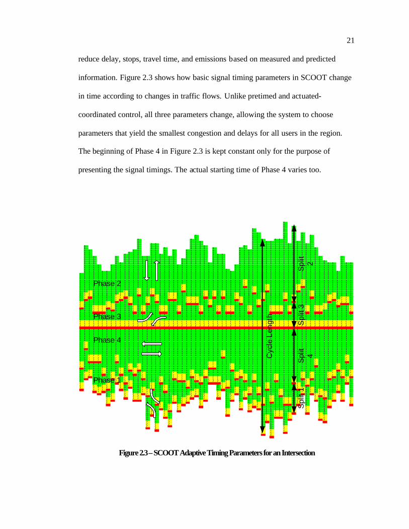
21
reduce delay, stops, travel time, and emissions based on measured and predicted
information. Figure 2.3 shows how basic signal timing parameters in SCOOT change
in time according to changes in traffic flows. Unlike pretimed and actuated-
coordinated control, all three parameters change, allowing the system to choose
parameters that yield the smallest congestion and delays for all users in the region.
The beginning of Phase 4 in Figure 2.3 is kept constant only for the purpose of
presenting the signal timings. The actual starting time of Phase 4 varies too.
III II I II I I
I I I I II I I I I I II I I I I I II I I I I I I I I I I II I I I I I I I I I I I I I I II I I I I I I I I I I I I I I I I I I II I I I I I I I I I I I I I I I I I I I I I I
I I I I I I I I I I I I I I I I I I I I I I I I I I II I I I I I I I I I I I I I I I I I I I I I I I I I I I I I I II I I I I I I I I I I I I I I I I I I I I I I I I I I I I I I I II I I I I I I I I I I I I I I I I I I I I I I I I I I I I I I I I I I I II I I I I I I I I I I I I I I I I I I I I I I I I I I I I I I I I I I I I I I I I I I II I I I I I I I I I I I I I I I I I I I I I I I I I I I I I I I I I I I I I I I I I I I II I I I I I I I I I I I I I I I I I I I I I I I I I I I I I I I I I I I I I I I I I I I I II I I I I I I I I I I I I I I I I I I I I I I I I I I I I I I I I I I I I I I I I I I I I I I I I I I II I I I I I I I I I I I I I I I I I I I I I I I I I I I I I I I I I I I I I I I I I I I I I I I I I I I I I I II I I I I I I I I I I I I I I I I I I I I I I I I I I I I I I I I I I I I I I I I I I I I I I I I I I I I I I II I I I I I I I I I I I I I I I I I I I I I I I I I I I I I I I I I I I I I I I I I I I I I I I I I I I I I I I II I I I I I I I I I I I I I I I I I I I I I I I I I I I I I I I I I I I I I I I I I I I I I I I I I I I I I I I I I I I II I I I I I I I I I I I I I I I I I I I I I I I I I I I I I I I I I I I I I I I I I I I I I I I I I I I I I I I I I I I I II I I I I I I I I I I I I I I I I I I I I I I I I I I I I I I I I I I I I I I I I I I I I I I I I I I I I I I I I I I I I II I I I I I I I I I I I I I I I I I I I I I I I I I I I I I I I I I I I I I I I I I I I I I I I I I I I I I I I I I I I I I
I I I I I I I I I I I I I I I I I I I I I I I I I I I I I I I I I I I I I / I I I I I I I I I I I I / I I I I I I I I I I II I I I I I I I I I I I I I I I I I I I I I I I I I I I I I I I I I I I I / I I I I I I I I I I I I / I I I I I I I I I I II I I I I I I I I I I I I I I I I I I I I I I / I I I I I I I I I I I I I / I I I I / I I I I I I / / I I I I I I I I I I II I I I I I I I I I I I I I I I I I I I I I I / I I I I I I I I I I I I I . I / I I / I I I I I I / . I I I I I I I I I I II I I I I I I I I I I I I / I I / I I I I I I / I I I I I I I I I I I I I I I / I I / I I I I I I / I I I I I I I I I I I II I / I I I I I I I / I I / I I / I I I I I I . I I I I / I / I / I I I I I I / I I . I I I I I I . I I / I I I I I I I I II / / I I I I I I / / I I / I I / I I I / / I I I I I I / I / I / I I / I I I . I / I I I I / I I I I I / I I I I / I I I II / / I I I I I / / / I I . I I . / I I / / I I I I I I / I / I / I I / I I I I I / I I I I / I / I I I / I I I / / I I I II / . I I I I I / / . / I I I / I / I I / / I I / / / I . I . I . I I / / I I I I / I I I I / I / I I I . I I I / / I / / II . I I I I I I / . I / I I I / I / I I . . I I / / / I I / I I I I I . / I I I / . I I I I . I / I I I I I I I / . / / / I/ I I I I I / I . I I / I I I / I . I I I I I I / / / I I / I I I I I I / I I I / I I I I I I I . I I I I I I I . I / / / I/ I I I I I / / I I I . I I I . I I I I I I I I . . . I I / I I I I I I . I I I / I I I I I I I I I I I I I I / I I / . . I/ I I / / / / / I I I I / I / I I I / / I I / I I I I / I . I / I / / I I I / I . I I / / / I / I I I / I / / / I I . I I /. I I / / / . / I I I I / I / I I I / / I I / I I I I / I I I / I / / I I I / I I I I / / / I / I I I / I / / / I I I I I /I I I / / / I . I I I I / I / I I I / / I I / I I I I / I I I / I / / I I I / I I I I / / / I / I I I / I / / I I I I I I /I I I . . . I I I I I I . I . I I I . . I I . I I I I . I I I . I . . I I I . I I I I . . . I . I I I . I . . I I I I I I .I I I I I I I I I I I I I I I I I I I I I I I I I I I I I I I I I I I I I I I I I I I I I I I I I I I I I I I I I I I I I II I I I I I I I I I I I I I I I I I I I I I I I I I I I I I I I I I I I I I I I I I I I I I I I I I I I I I I I I I I I I II I I I I I I I I I I I I I I I I I I I I I I I I I I I I I I I I I I I I I I I I I I I I I I I I I I I I I I I I I I I I I/ / / / / / / / / / / / / / / / / / / / / / / / / / / / / / / / / / / / / / / / / / / / / / / / / / / / / / / / / / / / / // / / / / / / / / / / / / / / / / / / / / / / / / / / / / / / / / / / / / / / / / / / / / / / / / / / / / / / / / / / / / // / / / / / / / / / / / / / / / / / / / / / / / / / / / / / / / / / / / / / / / / / / / / / / / / / / / / / / / / / / / / /. . . . . . . . . . . . . . . . . . . . . . . . . . . . . . . . . . . . . . . . . . . . . . . . . . . . . . . . . . . . . .I I I I I I I I I I I I I I I I I I I I I I I I I I I I I I I I I I I I I I I I I I I I I I I I I I I I I I I I I I I I I II I I I I I I I I I I I I I I I I I I I I I I I I I I I I I I I I I I I I I I I I I I I I I I I I I I I I I I I I I I I I II I I I I I I I I I I I I I I I I I I I I I I I I I I I I I I I I I I I I I I I I I I I I I I I I I I I I I I I I I I I I II I I I I I I I I I I I I I I I I I I I I I I I I I I I I I I I I I I I I I I I I I I I I I I I I I I I I I I I I I I I I II I I I I I I I I I I I I I I I I I I I I I I I I I I I I I I I I I I I I I I I I I I I I I I I I I I I I I I I I I I I I II I I I I I I I I I I I I I I I I I I I I I I I I I I I I I I I I I I I I I I I I I I I I I I I I I I I I I I I I I I I I II / I I I I I I I I I I I I I I I I I I I I I I I I I I I I I I I I I I I I I I I I I I I I I I I I I I I I I I I I I I I II / I I I I I I I I I I I I I I I I I I I I I I I I I I I I I I I I I I I I I I I I I I I I I I I I I I I I I I I I I I I II / I I I I I I I I I I I I I I I I I I I I I I I I I I I I I I I I I I I I I I I I I I I I I I I I I I I I I I I I I I I II . I I I I I I I I I I I I I I I I I I I I I I I I I I I I I I I I I I I I I I I I I I I I I I I I I I I I I I I I I I I II I I I I I I I I I I I I I I I I I I I I I I I I I I I I I I I / I I I I I I I I I I I I I I I I I I I I I I I I I I I I II I I I I I I I I I I I I I I I I I I I I I I I I I I I I I I I / I I I I I I I I I I I I I I I I I I I I I I I I I I I I II I / / / I I I / I I I I I I I I I I I I I I I I I I I I I I I / I I I I I I I I I I I I I I I I I I I I I I I I I I I / II I / / / I I I / I I I I I I I I I I I I I I I I I I I I I I I . I I I I I I I I I I I I I I I I I I I I I I I I I I I / II I / / / I I I / I I I I I I I I I I I I I I I I I I I I I I I I I I I I I I I I I I I I I I I I I I I I / I I I I I I / I/ I . . . I I I . I I I I I I I I I I I I I I I I I I I I / / I I I I I I I I I I I I I I I I I I I I I I / I I I I I I . I/ I I I I I I I I I I / I / I I I I I I I I I I I I I I I / / I I I / I I I I I I I I I I I I I I I I I I / I I I I / I I I/ I I I I I I I I I I / I / I I I I I I I I I I I I I I I / / I I I / I I I I I I I I I I I I I I I I I I . I I I I / I I I. I I I I / I I I / I / / / I I I I I I I I I I I I I I I . . I I I / I I I I I I I I I I I I I I I I I I I I I I I / I I II I / I I / I I I / I . / . I I I I I I I I I I I / I I / I I I I I . I / I I I I I I I I I I I I I I I I I I I I / . / I /I / / I I / I / I / I I / I / I I I I I I / I I I / I I / I I I I I I / / I I I I I I I I I I I I I / I / I I I / / I / I /I / / I I . I / I . I I . I / I I I I I I / / / I / / I / I I I I I I / / / I / I I I I / I I I I I / I / I I I / / I / I /I / . I I I I / / I / I I I / I I I / I I / / / I . / / . / / / I I I / . / I / I I I I / I I I / I / I / I I I / . I . / .I . I I I I . / I / I I I . I I I / I I . / / I I / / I / / / I I I . I / I / I I I I / I I I / I . / . I I I . I I I / II I I I I I / I / / I I I I I I / I I I . . / I . / I / / / I / I I I . I . I I I I . I I I / I I / I I I I I I I I / I/ I I I / I . / . / I I I I / I . I I I I I / I I . I . . . / / I I I I I I I I / I I I I I . / I / I I I I I I I I . I/ / I / / I / I / I I I I / I I / I I I I / I I I I I / / I I I I I I I I / I I I I I I / I . I I I I I I / I I/ / / / / I / I . I I / I / I I / I I I I . I I I I I / . I / I I / I / I / I I I I I I / / I / I I I I I / I I. / / / . I . I I I / / . I I / I I I I I I / I I I . I I / I I / I / I . I I / I I I . / I / I / I I I / I I. / . I I / I I / / I I I . I I I I I / / I I / I I / I / / I / I I I I / I I I I / I / I / / I I . I I. I / / / / . / I I I I I I I I I / / I / / I / . I / . I . I I I I / I I I I . I . / / / I / / I
I / / / / . I I I I I / I I / / . I / / I / I / I I I I I / I . I I I I I / . / I / / I/ / . / / I I / I I I / I / / . I / . I / I . I I I / I / I I / / I / I / I . I / / // . . . I I / I I I / I / / / . I . I I / I / I / I I / / I / I . I I / . . // I I / / I I . I / . / I / I / / / I . I I / / I / I I I / /. I I . / I / / . / I / / / / . I I I I . . I . I I I / .I I I / I / / . I / / . / I I I I I I I / / I I .I / I . I / / / . / . I I I I I I I / / I I
I / I / . . / . I I I / / I I / / I II / I / I / I I I / / I / . . / II . I / I . I / I / / I / / /I I . I I / I . . I / / /I I / I / I I . . // I / I . I I ./ / / I I I/ / . I I /. / / I /. / / // / .
. /.
Cyc
le L
engt
h
Spl
it2
Spl
it 3
Spl
it4
Spl
it 1
Phase 2
Phase 3
Phase 4
Phase 1
Figure 2.3 – SCOOT Adaptive Timing Parameters for an Intersection

22
The most widely deployed adaptive signal control systems in North America
are SCATS (developed in Australia) (Lowrie 1982), SCOOT (developed in the U.K.)
(Hunt et al. 1981), RHODES (Head et al. 1992) and OPAC (Gartner 1983)
(developed in the U.S.).
Other adaptive signal control systems include LA-ATCS (developed in the
U.S.) (Hu 2000), UTOPIA (developed in Italy) (Mauro and Di Taranto 1990),
PRODYN and CRONOS (developed in France) (Khoudour et al. 1991, and Boillot et
al. 1992). All of these adaptive signal control algorithms can be classified as either
2GC or 3GC. Essential operations and philosophies of the major systems deployed in
the U.S. are described below. The SCOOT system represents adaptive traffic control
in this research. For this reason, SCOOT is described in a separate section to provide
more details about its philosophy and operations.
2.1.3.1 SCATS
SCATS stands for Sydney Coordinated Adaptive Traffic System. SCATS is a
hierarchical adaptive signal control system installed in over 50 locations worldwide.
SCATS was originally developed for the New South Wales Roads and Traffic
Authority for application in Sydney and other Australian cities. In this system, signal
timings are adjusted in response to traffic data measured by stop line detectors.
SCATS minimizes travel time, stops (for light traffic), and delays (for heavy traffic).
Cycle length optimization aims to keep the degree of saturation below the target and
split optimization aims to minimize delay at intersections. Offset plans are selected
from a predetermined library based on traffic flow on the links. The system does not

23
determine signal timings in advance but it reacts to changes in traffic flows that
occurred in the previous cycle. The system can be loosely described as a feedback
control system (Lowrie 1982).
SCATS has a hierarchical control architecture consisting of two levels, strategic
and tactical (Lowrie 1992). At the strategic level, a ‘subsystem’ or a network of up to
10 intersections is controlled by a regional computer to coordinate signal timings.
These subsystems can link together to form a larger ‘system’ operating on a common
cycle time. At the tactical level, optimization occurs at the intersection level within
the constraints imposed by the regional computer’s strategic control. Tactical control
allows early termination of green phases when the demand is less than average and
for phases to be omitted entirely when there is no demand. All the extra green time is
added to the main phase or can be used by subsequent phases.
Field tests conducted in the U.S. showed that SCATS was efficient in
improving network performance. In Troy, Michigan the SCATS system reduced
travel time by 20% in the AM peak period and by 32% in the nonpeak period. The
system also reduced delays by 20% (Abraham 2000). In Oakland County, Michigan,
a 3.1-mile corridor was controlled by SCATS. The test results indicated that travel
time was decreased by 8.6% in the AM peak, by 7% in the PM peak, and by 6.6%-
31.8% in the nonpeak periods (Abdel-Rahim et al. 1998).
2.1.3.2 RHODES
RHODES (Real-Time Hierarchical Optimized Distributed and Effective
System) prototype was developed at the University of Arizona. As a hierarchical

24
system, RHODES has three levels, including dynamic network loading, network flow
control, and intersection control. RHODES proactively responds to stochastic
variations in traffic flow by explicitly predicting individual vehicle arrivals, platoon
arrivals, and traffic flow rates for the three levels. The optimization objectives can
minimize average vehicle delay, average queues, and number of stops (Head et al.
1992).
At the intersection control level, RHODES uses a dynamic programming-based
algorithm to make decisions on signal stages based on predicted vehicle arrivals,
coordination constraints, flow predictions, and operational constraints. At the
network flow control level, a model called REALBAND optimizes the coordination
of observed and predicted platoons in the sub-network. At the dynamic network
loading level, the slowly-varying characteristics of traffic flow are controlled. The
five core- logics in the RHODES prototype are intersection optimization logic, link
flow prediction logic, network flow optimization logic, platoon flow prediction logic,
and parameter and state estimation logic (Mirchandani and Head 2001).
RHODES has also been linked to the CORSIM traffic simulation software. A
simulation experiment was taken on an arterial with nine intersections in Atlanta,
Georgia. Compared to semi-actuated timing plans generated by PASSER and
TRANSYT-7F, RHODES reduced average vehicle delays by 50% (for low traffic)
and 30% (for high traffic) (Mirchandani and Head 2001).
RHODES has been implemented in several locations, including Tempe and
Tucson (Arizona), Santa Clara County (Sunnyvale, California), Seattle (Washington)
and Oakville (Canada). Field test results from Seattle, WA showed that RHODES

25
performed generally better or the same as optimized fixed-time plans in terms of
arterial travel times (ITT Industries 2002).
2.1.3.3 OPAC
Parsons Brinkerhoff Farradyne Inc., and the University of Massachusetts at
Lowell jointly developed OPAC (Optimized Polic ies for Adaptive Control Strategy)
(Gartner 1983). For optimization, the network is divided into subnetworks, which are
considered independently. OPAC transitions between two models: one for congested
networks and the other for uncongested networks.
In the uncongested model, the signal timings are determined one of two ways:
Fixed-time plans are obtained off- line, or a “virtual cycle” is calculated dynamically.
The level of local to network control can be configured by the user. The local signal
timings are based both on detected data (15 seconds) and predicted data (60 seconds).
These are implemented for a time-step (roll period) of 2-5 seconds. In the congested
model, OPAC considers the saturation flows and maximizes the number of vehicles
that can pass through an intersection. It also considers the critical links as those that
are on the verge of spillback. Except for the computation of cycle length, OPAC is
not controlled by a central computer. Hence, it can run autonomously if
communications to the central server fail.
In the late 1990s and early 2000, OPAC was deployed on Route 18 in New
Jersey, Reston Parkway, VA, and Vancouver, WA. Some of the tests done in the
simulation environment showed the benefits of deploying OPAC over existing
pretimed plans (Stallard and Owen 1998). Unpublished literature (Ghaman Undated)

26
reported that results from the field tests on the Reston Parkway in VA showed that
OPAC could improve traffic performance by 5 to 6%. Currently, OPAC is not fully
operational anywhere (Fehon 2005).
2.1.4 SCOOT
SCOOT (Split Cycle Offset Optimization Technique) is a centralized traffic
adaptive signal control system. SCOOT was developed in the UK in the early 1980s
by the Transport Research Lab (Hunt et al. 1981). SCOOT continuously measures
traffic volumes on all approaches to intersections in the network and changes the
signal timings to minimize a Performance Index (PI). This PI is a composite measure
of delay, queue length and stops in the network. These changes in signal timings are
small enough to avoid major disruptions in traffic flow, but frequent enough to allow
quick response to changing traffic conditions.
2.1.4.1 Working Principles
The principal publication on SCOOT is the original report presented by the
Transport Research Laboratory (Hunt et al. 1981). It describes the details of the
SCOOT philosophy. The system has been modified and enhanced several times since
then (Bretherton and Bowen 1990, Bretherton 1996, Bretherton and Bowen 1998).
The most recently developed version is called SCOOT MC3 (which stands for
Managing Congestion, Communications and Control). The traffic lab at the
University of Utah currently uses an older version, 4.2 (versions 4.5 and MC3 were
developed after version 4.2).

27
SCOOT’s most fundamental goal is to minimize a measure of effectiveness
called the PI (Performance Index) (Hunt 1981). The PI is a composite measure of the
average queue lengths and the number of stops at all approaches. To this end, real-
time traffic flow data must be obtained from detectors in the street. These data are fed
into a model that develops a Cyclic Flow Profile (CFP). It then projects platoon
movement and dispersion downstream. Figure 2.4 shows this prediction process
along a 300-meter road segment. In this way, SCOOT’s traffic model estimates the
accumulation of queues at each approach of an intersection. The model then estimates
the queue discharge when the signal allows traffic to proceed.
Several parameters are needed to allow SCOOT to model these activities with
sufficient accuracy to create an optimum signal timing plan. These model parameters
Measured arrival patterns Predicted arrival patterns
0 10 20 30 40 50 600 10 20 30 40 50 600 10 20 30 40 50 60
0 10 20 30 40 50 600 10 20 30 40 50 600 10 20 30 40 50 60 0 10 20 30 40 50 600 10 20 30 40 50 60
0 10 20 30 40 50 600 10 20 30 40 50 60
0 10 20 30 40 50 600 10 20 30 40 50 600 10 20 30 40 50 60
1800
1800
1800
0 10 20 30 40 50 600 10 20 30 40 50 600 10 20 30 40 50 60
0 10 20 30 40 50 600 10 20 30 40 50 600 10 20 30 40 50 60
Flo
w (p
cu/h
)
1800
1800
1800
1800
1800
1800
1800
0 m
30 m
120 m
210 m
300 m
0
0
0
0
0
0
0
Figure 2.4 – SCOOT Predictions of Downstream Flow

28
are start-up delay (SLAG), journey time (the average travel time from the detector to
the stop bar) (JNYT), saturation occupancy (a measure of the flow capacity through
the intersection) (STOC), and Maximum Queue Clear Time (the time it takes for a
link to discharge a queue reaching from the stop line to the upstream detector)
(QCMQ).
All of this information is used to develop optimum coordination plans, much in
the same way as the TRANSYT-7F software. SCOOT is often referred to as an “on-
line TRANSYT” because of this (Martin and Hockaday 1995). The signal timings
that are sent to the system reflect movement toward an optimum timing plan by
increasing or decreasing the cycle time, offsets, and cycles. When implementing these
timings, it is unwise to change the cycle lengths and offsets dramatically. Doing so
can have adverse affects on the behavior of drivers because the changes are
unexpected. The system therefore changes the offsets and cycle lengths by 4, 8, or 16
seconds. SCOOT allows faster change rates at higher cycle times.
SCOOT has three optimizers - one for cycle time, one for offsets between
intersections, and one for splits at each intersection. The split optimizer adjusts the
green split between the various legs of an intersection. A few seconds before the end
of each phase change, the optimizer is run to see whether early termination or an
extension of the phase would improve traffic. The optimizer makes two classes of
changes: temporary changes that are likely due to random variation in traffic flow,
and long term changes that are smaller and accumulate over time to accommodate
true traffic flow variations. The splits are also optimized to work within the offsets
determined by the offset optimizer.

29
The offset optimizer recalculates the offsets for each intersection at a
predetermined point in the cycle. The process involves a calculation to see if the
offset can be adjusted to improve progression between it and all adjacent
intersections. The accumulation of all of these changes occurs over time to
accommodate longer-term changes. The offsets are optimized to function within the
cycle time determined by the cycle time optimizer.
The cycle time optimizer recalculates the optimum cycle time according to a
critical node in the region. A region is a set of adjacent signals that operate at the
same cycle time to allow for maximum progression. A critical node is selected in
each region. This is generally the node that requires the maximum cycle time.
Once SCOOT is installed on a network, each link must be validated. The
validation process entails going out onto the street and making sure that SCOOT is
modeling the queues as closely as possible to the way they actually occur on the
street. Doing this ensures a proper signal timing plan and the best results. In the
SCOOT-simulation environment, validation requires many observations of simulated
traffic and relevant SCOOT outputs. SCOOT parameters are adjusted in an iterative
process so that SCOOT queues are as close as possible to queues from simulated
traffic.
SCOOT has several other features that give the system more flexibility. Similar
to fixed-time plans, which require adjustments to get it tuned on the street, SCOOT
needs fine-tuning during the initial setup.

30
2.1.4.2 Evaluation Studies
Several agencies have compared SCOOT’s performance to previous signal
control strategies. The benefits realized from SCOOT depend on the prior control
strategy and how well it was optimized.
The most recently published evaluation was performed by Companhia de
Engenharia de Trafego, the traffic engineering company responsible for managing
traffic in Sao Paulo, Brazil (Mazzamatti et al. 1998). The evaluation done in
Nijmegen, Netherlands compared SCOOT to fixed-time plans (Taale et al. 1998).
Before and after studies in Toronto, Canada also compared SCOOT’s performance to
coordinated fixed-time plans (Quan et al. 1993). Benefits in Beijing, China were
higher than the most of the others as SCOOT was compared to uncoordinated fixed-
time control (Peck et al. 1990). SCOOT benefits were higher when compared to
isolated vehicle actuation than coordinated fixed-time plans in Worcester, UK
(Hereford Department of Transport et al. 1986). Evaluations in London (Chandler
and Cook 1985), Southampton (Powell 1985) and Coventry in the UK also showed
significant benefits from SCOOT in the early 1980s. It should be noted, however, that
most of these results were not reported to be significant at a 95% confidence level.
Evaluations were also done in Santiago, Chile but were not expressed as percent
benefit and hence were not comparable to the other results.
Comparison with fixed-time control showed that SCOOT reduced delay and
travel time, thereby improving traffic network performance. Early evaluations in the
UK showed that SCOOT typically reduced delay by up to 33% and travel time by up
to 8%. The literature also indicated that validating SCOOT during installation is

31
extremely important. A nonvalidated SCOOT system in Nijmegen worsened system
performance, but when properly validated, it improved delay by 25% and travel time
by 11%.
However, some exceptions to SCOOT performance exist. A report
(Jayakrishnan et al. 2001) evaluated the SCOOT system in Anaheim, California using
“non- idealized” detectors which were placed 250 feet ahead of the intersection
approach stop line and only partially met the requirements of SCOOT. The field test
results showed that in some cases SCOOT performed worse than the baseline system
and in other cases SCOOT performed better. The variation range was within 10%.
Overall, the test did not show significant SCOOT benefits. The author indicated that
SCOOT was not beneficial due to the nonidealized detectors. Another reason may be
that minimal time was spent fine-tuning SCOOT’s parameters.
In addition to the field tests, SCOOT has been evaluated many times in the
simulation environment. Some researchers emulated SCOOT performance through a
continual time-sliced application of TRANSYT, an offline optimization program on
which the initial SCOOT program was based (Rakha and Van Aerde 1995, Liu and
Cheu 2004). These attempts, however, provide questionable findings because
SCOOT not only applies TRANSYT optimizations in real time, but also decides
when to apply these optimizations to minimize possible transients.
Real SCOOT-simulation modeling started in 1998 when the first SCOOT-
CORSIM interface was developed by Hansen and Martin at the University of Utah
Traffic Lab (UTL) (Hansen and Martin 1999). The authors compared SCOOT and

32
TRANSYT-7F performance on a small, 6- intersection network in an urban area. The
results showed that SCOOT can reduce delay and stops by up to 30%.
Research in the UTL continued with evaluations of SCOOT control in various
traffic conditions. One of the studies (Jhaveri et al. 2001) compared SCOOT
performance with fixed-time plans for a range of congestion intensities on a four-
intersection corridor. The results showed that most of SCOOT’s benefits (8 -13%)
come for volume/capacity (v/c) ratios between 0.7 and 0.9. The research showed that
SCOOT operates much like a fixed-time control once traffic becomes saturated.
Another study (Chilukuri et al. 2004) investigated the benefits of SCOOT
control during incidents. SCOOT performance was again compared to fixed-time
control. Incidents with durations of 15, 30, and 45 minutes were modeled in one
experimental and two real-world networks. The results showed that SCOOT
outperformed fixed-time control with benefits of up to 40% in total network delay,
travel time, and intersection delay.
In 2002 another interface between SCOOT and a micro simulation model was
developed. Feng and Martin (2002) developed a SCOOT-VISSIM interface on the
same basis as the previous SCOOT-CORSIM interface. The SCOOT-VISSIM
interface was used to evaluate SCOOT performance and the impacts of SCOOT bus
priority on buses and private vehicles under varying traffic conditions. These
conditions included three corridor congestion scenarios, three bus frequency
scenarios and two bus location scenarios. The study compared SCOOT control with
bus priority, SCOOT control without bus priority, and optimized pretimed signal
timings. A real-world corridor with nine intersections was also modeled to validate

33
the findings. The research found that SCOOT controls performed better than pretimed
control under noncongested conditions. All of the SCOOT controls reduced nonbus
traffic delay by 1.5 – 3 seconds (7% - 13%) per person per intersection and bus-
person delay by 1 – 9 seconds (3% - 33%). SCOOT control with bus priority was
slightly better then SCOOT control without bus priority.
Although most of the SCOOT-simulation research was done in the UTL, there
were a few outside studies that investigated SCOOT performance with other
simulation tools. Two of those studies were done as part of the PRIMAVERA project
(PRIority MAnagement for Vehicle efficiency, Environment & Road safety on
Arterials). In the first study (Fox et al. 1994), SCOOT was connected to AIMSUN2
(a traffic microsimulation program) and CLAIRE (an expert system for congestion
management). The idea was to pass detector data from AIMSUN2 to SCOOT, which
would return signal timings to the simulated traffic network. At the same time, link
congestion information from SCOOT was sent to CLAIRE. The CLAIRE program
was then used to recommend interventions via link control actions if necessary. The
interventions had to be translated into appropriate SCOOT parameter changes. There
was no publication available on the field tests of this method.
The second study (Fox et al. 1995) developed an interface program to link the
Italian simulation model NEMIS to the UK SCOOT system, allowing them to
interact. This interaction was part of the wider project’s goal in which co-operative
strategies that combine queue management, public transport priority and traffic
calming methods on urban arterial roads were developed. Traffic flows on the arterial
and surrounding network were collected automatically and passed to computers,

34
which rapidly calculated signal plans to minimize the overall travel time. Public
transport vehicle location systems were used to send data to these computers to let
them adjust the signal plans to ensure that public transport vehicles got priority when
they passed through intersections. The major benefits due to adoption of the
PRIMAVERA strategies in Leeds were a 10% reduction in travel time for buses and
improvements in safety due to ‘removal’ of the speeding vehicles on entry points to
the network.
Another SCOOT-simulation interface was developed in 1998 by Kosonen and
Bargiela (1999). This interface connected SCOOT control with HUTSIM
microscopic simulation model. The authors described a framework for a connection
between SCOOT and HUTSIM, but they did not conduct any comparison between
SCOOT and other traffic control systems. They reported that simulation somewhat
matched observed vehicle counts, but they did not perform any validity tests.
2.2 Review of the Studies on Ageing of Traffic Signal Timing Plans
Investigation of the deterioration of traffic control systems has drawn little
attention from traffic researchers over the last 20 years. Although embedded into few
research projects on traffic signal optimization (Park et al. 2000, Sunkari 2004,
Swayampakala and Graham 2005), deterioration of signal timings has not been
explicitly investigated.
2.2.1 Bell’s Research on Ageing of Fixed-Time Traffic Signal Plans
The key research conducted by Bell and Bretherton (Bell 1985, Bell and
Bretherton 1986) comprehensively quantified the disbenefits of aged pretimed traffic

35
signal systems. The authors used TRANSYT 8 (UK version) to simulate the
performance index (a composite measure representing the costs of traffic
performance) for deterministic traffic flows. The disbenefits of not updating pretimed
signal plans were calculated for various traffic networks. Traffic variability was
modeled with the Monte Carlo method through a series of random and uniform
changes to link flows.
The ageing disbenefits were estimated for both experimental and real networks.
The experimental results showed that the disbenefits of not updating grid networks
were one tenth of the average difference between base and aged link flows over the
entire network. The results from the real world showed that the disbenefits for grid
networks were around 3.8% per year, with up to four years between updates.
The study broke new ground, but was constrained by the computational
constraints of the mid-1980s. There are four major limitations of the study:
• Small traffic flow variations
• Unbalanced traffic flows between intersections
• No testing through microsimulation
• Unreliable ageing measure
Each of these limitations is commented on separately in the following
paragraphs.
Small traffic flow variations – Bell used coefficients from -10% to 10% to
represent uniform decreases/increases in background traffic demand for the whole
network. Similarly, coefficients from 5% to 25% were used as random fluctuations of
the turning movement proportions for each link. When experimental estimations were

36
compared to real traffic data, the author concluded that the range of the variations in
simulated flows was smaller than the range from real traffic. To avoid this mistake,
this study encompasses a wider range of the similarly constructed coefficients for
traffic demand and distribution.
Unbalanced traffic flows between intersections – The version of TRANSYT
used in the mid-1980s in the UK did not provide a tool for balancing traffic flows in
the network. For this reason, the conservation rule of traffic flows (analogue to the
first Kirchhoff's law - conservation of electric charge) was not satisfied. This means
that traffic flow on each link was separately changed (increased or decreased),
regardless of the changes in traffic flows on the upstream links. This approach could
potentially impact the final results of the disbenefits of aged signal timings. All traffic
flows in the network used in this study were balanced automatically after any change
in the flows.
No testing through microsimulation - The third limitation of Be ll's study is that
the results were evaluated with the model used to predict the differences. Ideally, if
the deterioration is evaluated properly, the differences between optimized and non-
optimized performances should be validated with separate simulations or an
analytical tool. In this research, microsimulation is selected to check the validity of
the differences obtained from macroscopic optimization models.
Unreliable ageing measure – The previous three limitations were either
obvious from Bell’s research scope (TRANSYT use only) or recognized by the
author (unbalanced flows and too small traffic variations applied). The fourth
limitation is implied in Bell’s research paper (1985), but is not recognized. However,

37
the author of this dissertation believes that this ageing measure is the reason for the
inconsistency between the results from the experimental study and the real-world data
from Bell’s study.
Bell developed two ageing measures (A and B) to express changes in traffic
flows on the network over the years. These measures are very similar. Measure A
considered total flows on the links between any two nodes in the network. Measure B
dealt with three link flows (left, through, and right) from the same link used for A
(one for each turning movement at the intersection). Consequently, the number of
links on the network is three times greater for Measure B than for Measure A.
The concept behind Measure B is denoted CF (Changed Flows) and explained
here. This measure was supposed to be a universal measure that shows how much
traffic in the network has changed since the last optimization of traffic signals. Bell
(1985) calculated Measure B (CF) as an average absolute difference between traffic
flows for aged traffic conditions and base traffic conditions, whereby:
N
FFCF
N
iab∑
=
−= 1 [2.1]
Where:
CF = Ageing measure of changed link flows
Fb = Base link flow (for all turning movement links) [veh/hour]
Fa = Aged link flow (for all turning movement links) [veh/hour]
N = Total number of links in the network (all turning movement links)
However, this measure by definition seems to be an unreliable indicator of link
flow changes. The measure might work for one type of change in link flows (increase
38
or decrease). However, when changes in link flows are triggered by simultaneous
changes in traffic demand and turning movement proportions, Measure B would not
be a reliable indication of the aged traffic conditions. One of the secondary objectives
of this research is to investigate the reliability of this measure.
2.2.2 Other Studies
The FHWA Primer (FHWA 1995) reported that improvement of coordinated
traffic signal timing plans reduces travel times by an average of 12%. This study also
gave an estimation of the benefits for several improvements in traffic signal
operations. The benefits range from 12% to 25%, depending on the traffic signal
operation conditions before and after improvement. However, in general this report is
more of a qualitative assessment than quantitative evaluation of the achieved benefits.
In 2000, Park et al. (2000) provided a more comprehensive assessment of the
direct Genetic Algorithm (GA) optimization within the CORSIM micro simulation
program. Two types of traffic demand changes were investigated. First, the mean
rates of demand for the network entry points were changed randomly to ±15% from
the base demand to account for changes in mean demand rates since CORSIM always
produces demand distribution around predetermined mean rates of demand. Second, a
10% increase over the entire network was modeled to account for systematic changes
in travel demand. This approach emulated the ageing of traffic signals. No explicit
modeling beyond CORSIM’s own stochastic variability was made to simulate
changes in turning movement proportions at the intersections. The study found that
optimizing timing plans for a 10% higher traffic demand on the network yields better

39
performance than optimizing for the current demand, if demand is expected to grow.
In other words, if demand is expected to grow, signal timings should be optimized for
higher demand and the benefits will increase over the long term. The benefits of
optimizing the timings for 10% higher demand surpass the cost of not optimizing the
timings for higher demand while the demand is still low.
An ITE study (Sunkari 2004) illustrated that user costs increase substantially if
timing plans are not updated at least every three years. This study also represents
qualitative assessment of benefits of retiming traffic signals without details for the
assumptions and methodology used to estimate these benefits.
Swayampakala and Graham (2005) investigated the optimal time between
traffic signal retiming. They analyzed more than 6,400 Synchro files representing
existing and future conditions at 13 signalized intersections. They concluded that
signals should be retimed every 18 to 30 months depending on the variability of
traffic volumes at the intersections. Microscopic simulation was not used in this
study.
2.3 Summary of Literature Review
The first section of the literature review introduces basic concepts of the three
most common types of traffic control. Pretimed, actuated, and adaptive controls are
described, with the most emphasis given to adaptive control. Four major types of
adaptive traffic controls deployed in the U.S. are described. Special emphasis among
adaptive controls is given to the SCOOT – the adaptive control used in this research.

40
SCOOT’s major working principles are described, along with a review of both field
and simulation tests of SCOOT installations.
The second part of the literature review presents summaries from a few studies
on the ageing of traffic signal systems. Special attention is given to Bell’s study (Bell
1985, Bell and Bretherton 1986) because this study has been the only study that has
explicitly investigated the ageing of traffic signals for the last 20 years. The major
limitations of Bell’s study have been listed along with proposed approaches to avoid
the same limitations in this research. Finally, a few other studies that have touched on
the same topic have been reviewed.
Summarizing the literature review on ageing of traffic signals, there is no
comprehensive study that investigates the ageing of signal timing plans using
macrosimulation and microsimulation analysis tools. Further, the last attempts to
investigate the reliability of macro optimization plans did not include variations in
turning movements. The methodology used 20 years ago to assess the ageing of
pretimed traffic signal plans was limited by the processing power available at the
time.

CHAPTER 3
RESEARCH METHODOLOGY
The first part of this chapter describes the concept of ageing (deterioration) of
signal timing plans. A method is proposed to measure the extent of the signal timing
plans’ ageing. The next part of the chapter presents the network and the set of
assumptions used to design simulation experiments. Selection of appropriate tools for
assessing the ageing of signal timing plans follows. This section represents a study
within the main research. It has its own literature review, methodology, results, and
discussion. The next part of the chapter deals with the main modeling process. It
describes modeling experiments for the three types of traffic control and validation of
the SCOOT model. The last part of the chapter summarizes the research methodology
and presents its findings.
3.1 The Concept of Ageing of Traffic Control Systems
The deterioration of traffic signal systems is a complex process. The two major
factors that influence the traffic signal systems’ deterioration over time are:
1. A traffic control regime does not have information about the current
traffic in the network that it is supposed to control
2. The traffic control system is unable to find the optimal control for traffic
in the network.

42
The first reason for poor traffic control is associated with the traffic control
system’s inability to gather updated traffic flow information from the road network.
Situations that keep the traffic control system from having sufficient information
about traffic conditions are: no detectors, too few detectors, faulty detectors, detector
data that is insufficient for good control, poor detector locations, etc. The second
reason is associated with the traffic control system’s inability to find the optimal
control based on the gathered information.
This research deals with both factors that influence the quality of a traffic
control regime. In the case of pretimed and actuated control, deterioration of control
regimes is mostly associated with the limited amount of traffic data available to these
systems. In the case of SCOOT, adaptive control deterioration might be associated
with both a lack of information from the detectors and the inability of the system’s
algorithm to cope with changed traffic flows. However, timeliness and accuracy of
traffic information fed into the system is crucial for all traffic control regimes.
Information on traffic flows and how closely they compare with estimated traffic
flows has a huge impact on the performance of traffic flows. In other words, the less
traffic flows deviate from the expected flows, the better the traffic control.
3.1.1 Variability of Traffic Flows
In general, a traffic control regime can perform suboptimally due to three basic
types of changes in traffic flows:
1. Short term changes result from sudden fluctuations in travel demand and
distribution lasting from several minutes to an hour (for example, a 15-minute

43
event-driven increase in traffic). They are stochastic and not recursive with
any recognizable pattern.
2. Medium term changes are mostly associated with diurnal or seasonal
changes in traffic flows resulting from various trip purposes, such as increase
in traffic demand during a peak period. They are a combination of stochastic
and deterministic factors in traffic demand.
3. Long term changes depict permanent changes in traffic demand, and
distribution and can be modeled as deterministic growth factors applied to
base traffic volumes.
These changes, along with their temporal natures, modeling approaches and coping
mechanisms, are summarized in Table 3.1.
We can distinguish between the performance losses in traffic control due to
traffic fluctuations, diurnal/seasonal traffic variations, and traffic growth based on the
classification of traffic flow changes. For each type of traffic change, there is a term
representing the ability of a traffic control regime to cope with the changes.
Flexibility, responsiveness, and adaptability refer to the system’s ability to cope with
traffic fluctuations, diurnal/seasonal traffic variations, and growth in traffic,
Table 3.1 – Changes in Traffic Flows and Associated Terms
Term Traffic Demand Coping Mechanism
Temporal Nature
Modeling Approach
Short Fluctuation Flexibility Temporary Stochastic
Medium Diurnal/Seasonal Change
Responsiveness Cyclical Stochastic & Deterministic
Long Growth Adaptability Permanent Deterministic

44
respectively. Although these three words can sometimes be used synonymously, there
is a bit of logic in associating each term with each type of traffic change.
1. Flexibility represents the ability of the system to cope with short term
changes. Although often used synonymously with adaptability, this term
assumes a short time in responding to changes and the ability to quickly
recover to the previous state.
2. Responsiveness, in this case, represents the ability of the system to cope
with diurnal and seasonal traffic variations. When variation occurs, the system
is supposed to adjust itself to the new conditions. This adjustment does not
have to be as fast as the one associated with the traffic fluctuations. A
responsive system should be able to recover to the previous conditions with
the same slower speed. The term “responsiveness” is used for medium term
changes because of the traffic-responsive signal systems that choose plans
based on pattern matching.
3. Adaptability represents the system’s ability to adjust to long term traffic
changes. This term is often used as a synonym for flexibility but it does not
involve any underlying meaning of the quickness of this process.
Ageing in this study is defined as the inability of a traffic control regime to
adapt to long term changes. Similarly, a traffic control system is inflexible if it does
not adjust to traffic fluctuations. Finally, a traffic control system is irresponsive if it
does not respond to medium term traffic variations. It seems that flexibility and
responsiveness can accommodate for some portion of ageing, but not all of it.

45
The term “ageing” is synonymous with deterioration or degradation over time.
However, ageing does not assume any reversibility. For example, a traffic signal
system can fail to perform optimally the day after it is installed because of high traffic
fluctuations. However, this does not mean the system has aged. If the system were
again able to perform optimally, then the earlier performance loss would be attributed
to the system’s unresponsiveness to varying traffic. However, if volumes were to
increase so that, regardless of traffic fluctuations and variations, two years later the
system never again reached optimal performance, then the system would have aged.
The ageing concept presented here considers only long term changes in traffic flows.
3.1.2 Measuring the Ageing of Traffic Signal Timing Plans
There are various ways to measure the success of traffic control. The major role
of traffic control, other than providing safe movement for conflicting traffic streams,
is to make the movements as efficient as possible. The number of stops, travel time,
delay time, pollutant emissions, and fuel consumption are all measures of the success
of the traffic control regime. In general, the goal is to keep all these measures as low
as possible. An increase in any of these factors represents a cost to society.
When traffic conditions change, signal timing plans (once optimized to yield to
the smallest impedance on traffic) need retiming or updating. Retiming of signal
timing plans represents a process in which signal timing parameters are chosen to
minimize costs for new traffic conditions. When this process is performed, signal
timing plans again become efficient and they improve the performance of the traffic
control regime. By measuring the differences in performance of a traffic control

46
regime before and after retiming, one can find the extent of deterioration of the traffic
control regime, or, more accurately, the deterioration of the signal timing plan. When
this process is performed in the field, it requires measuring or expert judgment of
vehicle delays, stops and queues before and after retiming takes place. In this
research, performance measures of control regimes are taken from simulation outputs.
The following subchapters describe how we deduce deterioration for pretimed,
actuated and adaptive traffic regimes.
3.1.2.1 Ageing of Pretimed and Actuated Traffic Control Regimes
Figure 3.1 shows a theoretical representation of the hypothetical relationship
between traffic control performance and change in traffic flows. Its purpose is to
represent the relationship between the set of factors that influence deterioration of
traffic signal regimes. It does not show actual results. This relationship can be applied
to single intersections and urban arterials, or networks. The X and Y axes represent
changes in traffic flows and a traffic control Performance Index (PI), respectively.
Point A in the figure represents the PI associated with an optimal timing plan during a
peak traffic period for base traffic conditions (Base Flows). If the traffic flows
increase or decrease, the PI, which is used as an objective function in the optimization
process, is supposed to increase or remain unchanged (if there is more than one
optimal PI).
If the traffic flows increase from the base traffic flows to the traffic flows
shown as ?8, the PI changes for two reasons. First, the existing timing plan becomes
obsolete and the PI increases by amount D2. Second, the ability of the road network

47
BaseFlows
∆1 ∆3 ∆4 ∆5
Base PI
NpNt
∆2
OpNt
D3
PerformanceIndex
Change in Traffic Flows∆6 ∆7
A
TimingPlan 1
∆8 ∆9 ∆10 ∆11 ∆12
TimingPlan 2
OptimizedPerformance
A’
TimingPlan 3
D2
A’’D1
D1'
NonoptimizedPerformance
D2'
D3'
C’
C’’
Figure 3.1 - Impact of the Traffic Changes on the Nonadaptive Traffic Controls
and traffic control system to cope with traffic demands decreases with the increase in
traffic flows by amount D3. These two processes work in the same direction when
traffic flows increase. However, if the traffic flows decrease, then the increase in PI
due to a suboptimal timing plan could be countered by the positive effects of the
decrease in traffic demand. Point C’ represents the PI with existing timing plans and
increased traffic flow. The PI produced for these conditions is labeled OpNt – Old
Plan New Traffic. Had the timing plan been optimized for new traffic, its PI would be
called NpNt – New Plan New Traffic. These conditions are represented by point A’.
The difference between OpNt and NpNt is labeled D2 and represents an
increase in PI, after a certain change in traffic flow, due to “suboptimal” signal
performance. Similarly, the difference between NpNt and Base PI (D3) represents an
increase in PI due to limitations in intersection (or network) capacity. This portion of

48
PI increase will exist, with an increase in traffic flows, regardless of whether the
timing plan is optimal. Finally, the total increase in PI (or total system degradation
after the change in traffic flow ?8) is represented as D1, which is the difference
between OpNt and Base PI.
The difference D2 can be interpreted as a benefit of updating the old timing
plan after a certain change in traffic conditions. Therefore, the percentage benefit of
updating a timing plan (ß) can be shown by:
%1002
×=OpNtD
β [3.1]
Where:
D2 = Measure of the benefits (reduction in PI) obtained by updating the timing
plan
OpNt = The PI of the old timing plan after a certain change in traffic flow (?8)
Similarly, the percentage disbenefit of not updating a timing plan (d) can be
calculated as:
%1002
×=NpNtD
δ [3.2]
where NpNt represents the PI of the new timing plan after a certain change in traffic
flow. These disbenefits, or opportunity costs, represent the loss associated with not
updating signal timing plans.

49
3.1.2.2 Ageing of Adaptive Traffic Control Systems
Figure 3.2 shows a hypothetical prediction of the ageing process for both
pretimed and adaptive traffic controls. Pretimed traffic and actuated control timing
plans are optimized in such a way that the optimal PI is achieved for the base traffic
state (Base Flow). If the traffic flow increases or decreases, the PI may increase.
Point B in Figure 3.2 represents the PI for the same traffic characteristics when an
adaptive control regime controls the traffic. The notation “Base ATCS PI” represents
ATCS performance (PI) for base traffic flow. Point B can be either below or above
point A.
The previous section shows how to assess the measure of the ageing of
pretimed and actuated traffic control regimes (D2). The system performance is
measured both before and after updating the signal timing plan to estimate the
decrease in system performance due to the obsolescence of the timing plan.
A similar procedure cannot be used to assess the ageing of an ATCS when the
ageing results from any type of traffic flow changes. This is because the ATCS
gradually changes signal timing plans by responding to changes in traffic flow. In
other words, there is only a single curve for ATCS performance in Figure 3.2. For
this reason, it is not possible, as with pretimed and actuated controls, to measure D2
after introducing a new timing plan. Instead, one can measure only the total
deterioration of the traffic control regime expressed as D1a.
D1a (total increase in PI for ATCS) includes both the potential deterioration of
the ATCS control regime and the road network’s inability to cope with changes in

50
Bas
eFl
ow∆1
∆3
∆4
∆5
Base
Pre
-Ti
med
PI
NpN
t
∆2
OpN
t
D3
Per
form
ance
Inde
x
Traf
fic F
low
∆6
∆7
A
Tim
ing
Pla
n 1
D2
D1a
B
∆8∆9
∆10
∆11
∆12
Tim
ing
Pla
n 2
A’’
B’
Bas
e A
TC
SP
I
D1
D1'
ATC
SP
erfo
rman
ce
Opt
imiz
edP
retim
edP
erfo
rman
ce
Non
optim
ized
Pre
timed
Perfo
rman
ceD2'
D1a’
D3'
ATC
S
B’’
A’C’
C’’
Tim
ing
Pla
n 3
Sub
optim
al T
imin
gs
Net
wor
k C
apac
ity
Figure 3.2 – Ageing of the Traffic Control Regimes with Change in Traffic Flow
Figu
re 3
.2 – A
gein
g of t
he T
raffi
c Con
trol
Reg
imes
with
Cha
nge i
n Tr
affic
Flo
w

51
traffic. For the sake of presenting the concept, the ATCS performance curve is placed
between optimized and nonoptimized pretimed performance curves (points B, B’, and
B’’). To assess the ageing of an ATCS, one would have to analyze the difference
between D1a and D3.
Ideally, the ATCS performance curve should overlie the optimized pretimed
performance curve and the difference between D1a and D3 should be zero. However,
this is not likely to be the case for actual ATCS implementations. Optimized pretimed
(or actuated) timing plans are likely to perform better than any ATCS for projected
constant traffic demand and distribution. In other words, if traffic demand and
distribution do not vary from the values used to optimize signal timing plans,
optimized pretimed or actuated timing plans will likely perform better than any
adaptive traffic control. Therefore, ATCS performance is likely to be represented by a
curve (in Figure 3.2), which is above the hypothetical optimized performance curve
for pretimed signals. An assumption used here is that traffic flows remain constant
throughout the period of analysis.
The major challenge is to recognize a trend in ATCS performance which would
imply an influence of changes in traffic flow on ATCS performance. The general idea
is to look for differences between D1a and D3 to detect any deterioration trend in
ATCS performance.
The difference between ATCS PI and PI of pretimed control is equal to B-A for
base traffic flows. If ATCS does not deteriorate at all, this difference should remain
constant or decrease for any further change in traffic flow. One should not forget that
performance of any of the traffic control regimes will worsen with an increase in

52
traffic flow. However, even if the ATCS is worse than pretimed performance for all
ranges in traffic flows, it should keep pace with optimized pretimed signal timing
plans.
Therefore, if the difference between ATCS performance and pretimed
performance does not increase with changes in traffic flows, one can say that the
ATCS does not deteriorate. Otherwise, it can be said that ATCS ages with changes in
traffic flows. Mathematically, if we assume that D1a is greater than D3, the following
inequality shows a condition for the existence of the ATCS ageing:
[3.3]
Or
[3.4]
In other words, if the difference between these two measures increases over
time, we can say that an ATCS deteriorates or ages. If the ratio between (D1a-D3)
and (D1a’-D3’) is one, then the ATCS does not age. However, this ratio should never
be greater than one because that would mean that ATCS improve performance with
increase in traffic flow. In Figure 3.2, D1a’ – D3’ = B’’ – A’’ represents the difference
for changed traffic flows for ∆10, while D1a – D3 = B’ – A’ is the difference for ∆8.
Since the former term is greater than the latter, we could say, if the results were
obtained from the simulation, that the ATCS ages. If there is ageing of ATCS, the
percentage of ATCS ageing (?) can be expressed as:
( ) ( )'' 3131 DDDD aa −<−
( )( ) 1
'' 31
31 <−−
DDDD
a
a

53
[3.5]
In general, the entire process of determining ? requires many traffic simulations
with controlled traffic flow inputs. This enables estimation of the aforementioned
measures D1, D2, D3, and D1a. The analysis of the measures requires statistical
testing for the difference between the measures. Once these measures are estimated, it
is possible to assess the potential deterioration of ATCS. The situation presented here
is the simplest case. If the differences between ATCS and pretimed PIs vary,
additional tools can be necessary to characterize the ageing process. The
methodology for estimating the ageing of ATCS presented in this section is original
and represents one of the contributions of the dissertation.
3.1.3 Selecting a Performance Measure
There are various ways to measure the performance of traffic control regimes.
The number of stops, travel time, delay time, pollutant emissions, and fuel
consumption are all traffic control regime measures. In general, the goal is to
minimize these measures. An increase in any of these measures represents a cost to
society. The PI from Synchro optimization software serves as the performance
measure. The PI is a composite measure of delay time and stops, which are two of the
most important MOEs for undersaturated traffic conditions (Husch and Albeck 2003
(I)). It represents the objective function in Synchro optimization and takes the form:
360010
SDPI ⋅+= [3.6]
( )( ) %100
''1
31
31 ×
−−
−=DDDD
a
aγ

54
Where:
D = Total delay (hours) per hour
S = Total number of stops per hour
10 = Weighting factor for stops
In order to make sure that the pretimed curves in Figures 3.1 and 3.2 represents
the best timing plans possible, the performance measure used as an objective during
the optimization of the timing plans must also be used to assess deterioration of those
plans. Any other measure would introduce uncertainty about the quality of the
optimized timing plans.
However, the PI used in SYNCHRO (a similar PI is used in TRANSYT-7F)
has some weaknesses. One of the major weaknesses results from the inability of some
simulation programs to account for delay and stops of those vehicles that did not
leave the network by the end of a simulation run. Another similar problem comes
from the fact that most types of simulation software do not account for the delays
experienced by vehicles that are not able to enter the network (due to congested
traffic conditions at the entry point). For this purpose, two additional measures of
effectiveness (MOEs) are gathered for each simulation run. The first measure is
network throughput. This measure represents a ratio between the number of exited
vehicles and the number of entered vehicles. The second measure is input ratio. This
measure is a ratio between the actual number of entering vehicles and the number of
vehicles intended to enter. These two ratios are usually around 99-100% percent.
However, when traffic conditions are saturated, more vehicles are locked in the

55
network by the end of the simulation and these ratios drop by a few percentages. In
such situations, these ratios are reported and the reliability of the PI is questioned.
3.2 Design of the Simulation Experiments
3.2.1 Experimental Grid Network
The design of the experiments was motivated by a need to set up a highly
experimental approach. There were several requirements that had to be satisfied for
the experimental network:
• The network was supposed to be like a real-world network with a complex
geometrical layout. A single arterial with 4-5 intersections would not
challenge optimization from any optimization software. Deterioration of one
(critical) signal at such a network would possibly cause more harm to the
performance of the whole system than if the network were simple.
• Traffic flows were supposed to be high enough that the benefits of
optimization would be gained either for an increase or a decrease in traffic
demand. The same applies for turning movement proportions.
• Traffic flows and turning movement proportions were supposed to be equal
(for most of the links) and symmetrical. As such, they represent controllable
variables that enable the development of a cause-effect relationship in the
postexperimental analysis.
• When selecting a test network for assessing the ageing of signal timing plans,
findings are needed that are not associated with particular road and traffic
conditions. Case studies can be difficult to generalize.

56
A grid urban network (the kind found in most urban districts) represents a
experimental grid network. Figure 3.3 shows a nine-node experimental grid network
with base traffic volumes. All links in the network are between 800 and 1000 feet
long, representing intersection spacing common for some urban districts (e.g., Salt
Lake City, UT). Two central arterials have three lanes in each direction, while four
peripheral arterials have two lanes in each direction. All intersection approaches have
250-foot left turn pockets and 150-foot right turn pockets.
Figure 3.3 - Test Bed Network with Base Traffic Flows (Synchro 6)

57
Pretimed and actuated coordinated controls are modeled separately. There was
no need to model actuated uncoordinated control considering the short spacing
between intersections and high coordinatability factors (Husch and Albeck 2003 (I)).
For pretimed and SCOOT controls, all intersections have signals with four major
phases: two for leading left turn movements and two for major through movements.
Actuated-coordinated control deploys eight phases instead of four. Operations of
actuated control with only four phases would limit performance of this control type.
The phases allow no permitted left turns. Right turns on red are available for all right
turn movements.
Base flows at the network entry points are 700 veh/hour for 2- lane arterials
and 800 veh/hour for 3-lane arterials. These flows are multiplied by 1.7 for all
northbound and eastbound approaches to model directional peak traffic demand. Free
flow speeds are 35 mph for 2-lane arterials and 45 mph for 3-lane arterials. Heavy
vehicles contribute 2% of the total traffic demand. There are no peaks in demand
flows and peak demand is constant during the peak hour. All turning movement
proportions in the network are equal for the base traffic conditions. All approaches
have 78% through traffic and 11% left and right traffic. This enables the modeling to
capture the relationship between changes in turning proportions and ageing of timing
plans.
All intersections are assumed to be fully coordinated within the network. The
intersection of two 3- lane arterials has a zero offset. However, the base traffic
conditions governed one of the peripheral intersections (intersection of 1011 and
58
1301 arterials in Figure 3.3) to become the critical intersection. There is no pedestrian
or transit traffic.
3.2.2 Traffic Demand and Distribution Scenarios
There were two aspects of assessing the ageing of timing plans through
simulation: deterministic and stochastic. The deterministic aspect is used for both
selection of appropriate simulation tools and assessment of the ageing of traffic
control regimes. The stochastic aspect is used only for the latter. The deterministic
aspect is introduced here. The stochastic aspect is introduced later in this chapter in
the section that describes the major modeling process.
Uniform deterministic traffic demand and distribution used 21 scenarios to
emulate the ageing of the link traffic flows. This approach was used to constrain the
number of controlled variables and provide explainable relationships between
changes in link flows and performance of traffic control regimes.
Two major aspects of changes in link traffic flows are assessed: total traffic
demand in the network (traffic flows at the entry points) and distribution (turning
movements at the intersections). Twenty-one scenarios were developed to emulate
variation in the link traffic flows. The first scenario represents the base traffic
conditions. Volumes and Levels Of Service (LOS) are shown in Figure 3.3.
Scenarios 2 to 11 represent changes in traffic demand. Traffic flows at the
entry points were decreased and increased by 5, 10, 15, 20, and 25% with respect to
base input flows. The turning movements for these 10 scenarios remain unchanged.
These scenarios emulate the increase or decrease in total network traffic growth. The

59
same increase and decrease factors are applied to all entry flows in order to capture
the influence of deterministic change in traffic demand on the ageing of signal timing
plans.
Scenarios 12 to 21 represent the change in distribution of the base traffic
flows. The traffic demand for these scenarios remained unchanged. These scenarios
were selected to emulate long term changes in turning movement flows at the
intersections. All turning movements (left and right) at each intersection were
decreased and increased by 10, 20, 40, 60, and 80% with respect to base turning
movements.
3.3 Selection of Proper Tools for Assessing the Ageing of Traffic Control
The concept of ageing of pretimed and actuated traffic control regimes is
presented in the first part of this chapter. Figure 3.1 illustrates the concept. A crucial
assumption is that optimized signal timing plans perform better than old outdated
timing plans. However, this is not always the case. Optimized timing plans that are
applied in the field or within simulation sometimes perform worse than non-
optimized timing plans. A major reason for this contradiction is the inability of the
macroscopic optimization tools to model traffic conditions properly. This inability is
largely impacted by two factors. The first factor is the quality of the underlying traffic
model (or, more precisely, the set of models) used by a macroscopic optimization tool
to emulate real-world traffic conditions. The second factor is adjustments to this tool
that have to be made to model field traffic conditions as closely as possible.
Adjustments of parameters that influence performance of the traffic model are made

60
through calibration and validation. Park et al. (2001) have shown that timings
optimized by an optimization tool based on a macroscopic model (TRANSYT-7F)
give inconsistent results when tested through micro simulation (CORSIM).
The following chapters introduce the definitions of different traffic analysis
tools, their differences and reasons for inconsistencies. A short review of previous
studies about microscopic and macroscopic simulation tools is given. Finally, the
reliability of macroscopically optimized timing plans used in microscopic simulation
models is assessed.
3.3.1 Traffic Analysis Models
The major difference between microscopic and macroscopic traffic models lies
in the different approaches they use to model traffic behavior in the real world. The
following definitions describe macroscopic, microscopic, and optimization tools.
Macroscopic simulation models are based on the deterministic relationships of
flow, speed, and density of the traffic stream. Simulation in these models is done
section-by-section rather than for trajectories of individual vehicles. The advantage of
macroscopic tools is that they are simpler and require less time to obtain the results of
the simulation.
Microscopic simulation models simulate the movement of individual vehicles
based on car- following and lane-changing theories. Each vehicle, with pre-
determined destination, vehicle type and driver characteristics, is tracked through the
network over small time intervals (1 second or less). Simulation results are much
more realistic than those from macroscopic models. However, computer time and

61
storage requirements for these models are large, usually limiting the network size and
the number of simulations that can be completed.
Traffic signal optimization tools are tools designed to develop optimal signal-
phasing and timing plans for isolated intersections, arterial streets, or networks. These
tools usually calculate capacity and optimize cycle lengths, splits, offsets, and phase
orders for traffic signals.
Optimization processes are complex and involve several parameters. Cycle
lengths, splits and offsets are all interconnected and they all have to be considered
during the optimization. This increases the number of possible alternatives to test for
given traffic conditions. This largely increases the time necessary to perform
optimization. The time necessary to test one signal timing alternative (cycle length,
splits, offsets) is a critical component of the optimization process. For this reason,
optimization tools use macroscopic models to evaluate the effectiveness of various
signal timing alternatives. When there is a trade-off between accuracy (microscopic
models) and efficiency (macroscopic models), optimization tools generally choose
the latter.
3.3.2 Review of Past Research
Investigation of the reliability of macroscopically optimized timing plans in
microscopic environments has drawn little attention. Park et al. (2001) evaluated the
reliability of TRANSYT-7F optimization schemes for both uncongested and
congested conditions. They compared TRANSYT-7F’s MOEs to those resulting from
CORSIM’s output using the same TRANSYT-7F timing plans. This is the first

62
explicit approach of assessing macroscopically optimized timing plans within a
microsimulation environment. Comparing the performance measures from
TRANSYT-7F and CORSIM, they reported a high correlation of MOEs for the
uncongested condition and a low correla tion for the congested condition. In both
cases, the performance measures for the macroscopic and microscopic models were
quite different. They associated these differences to a low fidelity traffic model
within TRANSYT-7F.
Rouphail et al. (2004) recognized the need for a better optimization tool to
evaluate performance measures for microscopic simulations. They developed direct
CORSIM optimization, a type of stochastic optimization, using the Genetic
Algorithm (GA) method for optimization of performance measures. The findings
showed that direct optimization consistently provided better MOEs than TRANSYT-
7F strategies, even though the best TRANSYT-7F strategies were selected based on
their performance in CORSIM, not in TRANSYT-7F.
Park et al. (2004) provided a more comprehensive assessment of the direct GA
optimization within the CORSIM micro simulation program. This time not only
TRANSYT-7F optimization schemes were compared with GA optimization, but the
performance of the GA was investigated for changes in traffic demand. Two types of
change were investigated. First, the mean rates of demand for the network entry
points were changed randomly to ±15% from the base demand. This approach was
used to account for changes in mean demand rates since CORSIM always produces
demand distributions around predetermined mean rates of demand. Second, a 10%
increase over the entire network was modeled to account for systematic changes in

63
travel demand. This approach emulated the ageing of traffic signals. No explicit
modeling beyond CORSIM’s own stochastic variability was made to simulate
changes in turning movement proportions at the intersections. This study also found
that GA optimization is better than TRANSYT-7F in the CORSIM environment and
performs similarly to TRANSYT-7F in the TRANSYT-7F environment. The results
showed that GA plans are more reliable for the changes in mean rates of traffic
demand.
Lee et al. (2004) investigated the performance of CORSIM, SimTraffic, and
Synchro 4 for application to diamond interchanges for three performance measures:
cycle length, average delay, and total stops. The research showed that the two
microscopic models performed similarly, but were different from the macroscopic
program Synchro. The study also found that SimTraffic modeled conditions more
restrictively than the other two tools in some situations.
In summary, studies have compared the performance of micro- and macro-
simulation tools. Discrepancies between micro- and macrosimulation tools for the
same timing plans have been recognized. There follows a comprehensive evaluation
of the reliability of the most popular signal optimization tools using the most popular
micro simulation tools. The objective of this portion of the research is to investigate
the reliability of timing plans optimized by Synchro and TRANSYT-7F in the micro-
simulation environments of CORSIM, SimTraffic, and VISSIM.

64
3.3.3 Basic Review of the Macro- and Microsimulation Tools Used
According to Tarnoff and Ordonez (2004), TRANSYT-7F and Synchro are the
most popular traffic control optimization tools among traffic signal practitioners in
the U.S. For this research, the author investigated the reliability of timing plans
derived by Synchro and TRANSYT-7F, which are tested by their implementation in
stochastic microsimulation.
The same survey (Tarnoff and Ordonez 2004) recognized SimTraffic and
CORSIM as two of the most popular micro simulation tools. Tian et al. (2002)
acknowledged CORSIM, SimTraffic and VISSIM as three of the most popular types
of microsimulation software in the U.S.
There have been numerous studies comparing the performance outputs from
various macro and micro simulation tools (Park et al. 2001, Lee et al. 2004, Tian et
al. 2002, Bloomberg and Dale 2000, Mystkowski and Khan 1999, and Trueblood
2005). Various micro- and macrosimulation tools rely on different traffic behavioral
models. They also use different ways to report MOEs from their models.
Consequently, they also report delays and stops in different ways. The following
paragraphs provide the most essential descriptions for each traffic simulation model.
The focus is on delays and stops produced by each tool as the major elements of the
PI.
Synchro (Version 6) is a macroscopic, deterministic simulation and
optimization model used mostly for the optimization of coordinated and
uncoordinated traffic signals. Synchro computes total delay (used as part of the
optimization objective) as a sum of the traditional control delay and blocking delay

65
(Husch and Albeck 2003 (I)). The delay is estimated based on queue polygon with
multiple percentile volume scenarios. Synchro calculates the percentage of stopped
vehicles based on TRANSYT-7F’s relationship between vehicle delays and percent
of stops (Husch and Albeck 2003 (I)). Lee et al. (2004) state that Synchro considers a
vehicle stopped when its speed is less than 3 m/s (10 ft/s).
TRANSYT-7F (Version 10) is also a macroscopic, deterministic simulation and
optimization model. Version 7F is an American version based on the original British
software. The TRANSYT traffic model is known as one of the best macroscopic
traffic models (Hale 2005). TRANSYT-7F computes total delay as a sum of total
uniform and random delays, well-known concepts of delay from analytical models.
Total number of stops in TRANSYT-7F is calculated as a sum of the stops for
different delay types. Number of stops for each delay type is based on the delay-stop
look up table.
Delay is usually defined as the entire amount of time spent not traveling at the
prevailing cruise speed. Although Synchro and TRANSYT-7F can estimate these
delays, they cannot explicitly trace the trajectories of individual vehicles to obtain
accurate delays. Similarly, the numbers of stops they estimate are only an
approximation of the “real” number of stops.
CORSIM (Version 5.0) is a stochastic microscopic simulation program
for urban traffic developed by the FHWA (1999). CORSIM reports delays and stops
by link. Delay time per vehicle is defined as an average delay on a link for each
vehicle, calculated by taking the total delay of all vehicles that have traversed the link
and dividing it by the number of vehicles. Stop percentage is defined as a ratio of the

66
number of vehicles that have stopped at least once on a link to the total number of
vehicles on the link. A vehic le is considered to be stopped when its speed is less than
3 feet/second (FHWA 1999).
SimTraffic (Version 6) is a stochastic and microscopic simulation program that
is closely tied to Synchro. SimTraffic incorporates the vehicle and driver parameters
developed by the FHWA for use in traffic modeling (Husch and Albeck 2003 (II)).
These parameters are basically the same as CORSIM’s parameters, with a few
exceptions (Husch and Albeck 2003 (II)). SimTraffic calculates total delay as the sum
of the ratios between actual vehicle slowdown (the difference between maximum link
speed and actual speed) and maximum link speed for all time slices of 0.1 sec. Total
delay also includes all time spent by denied entry vehicles while they are waiting to
enter the network. SimTraffic adds a stop to the total number of stops whenever a
vehicle's speed drops below 10 ft/s (3 m/s). Several studies (Lee et al. 2004,
Trueblood 2005, Husch and Albeck 2003 (II)) have found that CORSIM and
SimTraffic produce comparable performance outputs when calibrated properly.
VISSIM (Version 4.10) is another stochastic and microscopic simulation that
has recently been widely accepted in the U.S. Delay is measured in VISSIM as the
difference between free flow travel time and actual travel time on the user-defined
segments. These segments can be automatically created for the intersection delay
statistics or for delay on the entire network. VISSIM defines the number of stops
within the queue as the total number of events when a vehicle enters the queue
condition. The queue conditions are adjustable and the default value is 4.55 ft/s (1.4
m/s) (PTV AG 2005).

67
3.3.4 Optimization and Simulation in Macro- and
Microsimulation Tools
Figure 3.4 shows a simplified flowchart of major objects and processes for the
evaluation of optimization schemes in a microsimulation environment. Two different
approaches are examined in this research. In the first, the reliability of timing plans
from two macroscopic optimization tools is examined within three microscopic
simulations. This type of optimization is termed Indirect Optimization. In the second
approach, candidate plans from TRANSYT-7F’s GA optimization procedure are
evaluated through Direct CORSIM optimization.
First, the same 21 link flow scenarios, designed for assessing the ageing of
traffic control regimes, are used to evaluate the performance of the optimized timing
plans within micro and macro simulation tools. These scenarios are modeled in MS
Excel and account for various traffic demands and distributions. An Excel file is
designed to enable the selection of traffic demand and distribution, balancing of link
flows, and preprocessing output for peak hour volume data in a “*.csv” file with the
Universal Traffic Data Format (UTDF). The UTDF is a standard specification for
transferring data between various software packages (Husch and Albeck 2003(I)).
In the next step, the preprocessed volume data were imported into the base
Synchro file. When new volumes are imported into the old Synchro file (timings are
not changed), this corresponds to a situation in which signal timings are not adjusted
to the volumes: namely, the ageing of the timing plans. This type of Synchro file was
saved for further analysis as a Non Optimized (NO) file. Then, the optimization
process within Synchro was executed.
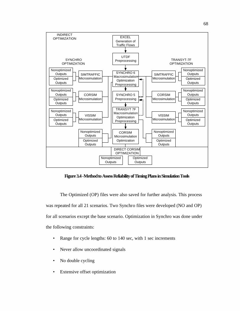
68
SYNCHRO 5Preprocessing
CORSIMMicrosimulation
EXCELGeneration ofTraffic Flows
SYNCHRO 6Macrosimulation
OptimizationPreprocessing
VISSIMMicrosimulation
TRANSYT 7FMacrosimulation
OptimizationPreprocessing
UTDFPreprocessing
SIMTRAFFICMicrosimulation
CORSIMMicrosimulation
VISSIMMicrosimulation
SIMTRAFFICMicrosimulation
CORSIMMicrosimulation
Optimization
NonoptimizedOutputs
OptimizedOutputs
NonoptimizedOutputs
OptimizedOutputs
NonoptimizedOutputs
OptimizedOutputs
NonoptimizedOutputs
OptimizedOutputs
NonoptimizedOutputs
OptimizedOutputs
NonoptimizedOutputs
OptimizedOutputs
SYNCHROOPTIMIZATION
TRANSYT-7FOPTIMIZATION
DIRECT CORSIMOPTIMIZATION
NonoptimizedOutputs
OptimizedOutputs
NonoptimizedOutputs
OptimizedOutputs
NonoptimizedOutputs
OptimizedOutputs
INDIRECTOPTIMIZATION
Figure 3.4 - Method to Assess Reliability of Timing Plans in Simulation Tools
The Optimized (OP) files were also saved for further analysis. This process
was repeated for all 21 scenarios. Two Synchro files were developed (NO and OP)
for all scenarios except the base scenario. Optimization in Synchro was done under
the following constraints:
• Range for cycle lengths: 60 to 140 sec, with 1 sec increments
• Never allow uncoordinated signals
• No double cycling
• Extensive offset optimization

69
• No lead/lag phasing optimization
• Search for the best timing plans
• 60-minute analysis period
The next step was to export the OP and NO Synchro files into micro-
simulation tools. Powerful Synchro transfer features were used to accomplish this.
Synchro 6 has a direct connection to SimTraffic 6, its microsimulation counterpart.
Synchro 6 also offers simple data transfer to CORSIM software. The transfer of data
to VISSIM had to go through a series of UTDF files (volume, timings, phasing, lanes,
layout). VISSIM uses a TEAPAC preprocessing tool called PRESYNCHRO to read
the UTDF files and to build its own network with all relevant volumes, timings, and
phasing data.
Although Synchro 6 was used as a major transfer tool between macro- and
microsimulation tools, its previous version, Synchro 5, was used to export- import to
TRANSYT-7F. Synchro 6 does not support export to TRANSYT-7F. Therefore, NO
Synchro files were first saved as Synchro 5 files and then exported to TRANSYT-7F.
These files were then used for macroscopic TRANSYT-7F analysis and optimization.
The first new set of OP files was generated from the TRANSYT-7F optimization.
Then these files with TRANSYT-7F signal timings were imported back into Synchro
5. Once again, the new Synchro 5 (TRANSYT-7F optimized) files were saved as
Synchro 6 files and they were ready for new transfers to the three micro simulation
tools. The TRANSYT-7F optimization was done based on input parameters from the
Synchro 5 files, so its limitations were inherently the same as the listed Synchro 6
optimization constraints.

70
For the evaluation of the Direct CORSIM optimization, the GA procedure
within TRANSYT-7F provides candidate plans to CORSIM. CORSIM executes runs
with the GA plans and delivers performance measures. These, in turn, are used to
generate new timing plan candidates through the GA procedure (Hale 2005). The
entire optimization process continues until convergence, or until a defined number of
iterations is complete. This is a new feature of TRANSYT-7F and its authors claim
that it is the best way to optimize timings for CORSIM performance. This
optimization is used in this study to investigate and compare its performance with a
traditional indirect-optimization approach.
For the Direct CORSIM optimization, the base-case timings for two initial
optimizations were imported into the other 20 CORSIM files describing 20 scenarios.
These files were saved as NO CORSIM files. Each of the 20 files was then optimized
twice using Direct CORSIM optimization. GA optimization performance largely
depends on the initial timing plans (Hale 2005). For this reason, the authors have
executed optimization for two initial timing plans. The first was the TRANSYT-7F
macroscopically optimized timing plan through the Hill Climbing procedure. The
second was the optimized timing plan through the Direct CORSIM optimization.
3.3.5 Simulation Runs
Ten simulations were performed for OP and NO Synchro 6 files within each
microsimulation software for each scenario. The same was repeated for OP and NO
TRANSYT-7F files. Each microsimulation was an hour long with 5 minutes of
seeding time. The 10 runs for each scenario used the same starting random seed

71
numbers for the corresponding microsimulations. Ten runs have been shown to be
enough for any of the microsimulation tools if the traffic demand (based on the HCM
V/C ratio) does not exceed or come close to 1.0 (Tian et al. 2002). Since all three
simulation tools had V/C ratios of less than one for most scenarios, they capture
reliable performance measures from the microsimulation outputs. In total, more than
2460 one-hour simulation runs were accomplished for the evaluation of indirect
optimization.
Forty optimization runs were conducted for the Direct CORSIM optimization:
two for each scenario based on two initial timing plans. Each run took about 6-7
hours. The parameters used in the GA optimizations were:
• Cycle length, splits and offsets were optimized (no phasing optimization)
• Lower cycle length was 60 sec, upper cycle length was 90 sec, original cycle
length was either 60 sec (optimal base cycle length from Direct CORSIM
optimization) or 66 sec (optimal base cycle length from TRANSYT-7F Hill
Climbing optimization)
• The Optimization objective function was Total Delay
• All default values were used for GA parameters, except for maximum number
of generation which was increased from 20 to 100 and population size, which
was increased from 10 to 20
The next step was to check the reliability of timing plans optimized through
Direct CORSIM optimization. This was necessary because Direct CORSIM
optimization evaluated alternative signal timings for only one simulation random seed

72
number. However, simulation results are valid only if they hold for several random
seed numbers of the same simulation.
For each scenario, 100 one-hour CORSIM runs were performed for three cases:
NO timing plans and two sets of OP timing plans with different initial timings. In
total, 6,100 one-hour CORSIM runs were performed.
3.3.6 Results of the Assessment of Simulation Tools
The following subsections present the results of the evaluation of
macroscopically and microscopically (Direct CORSIM) optimized timing plans when
used in microsimulation. The results are divided into two sections: uniform changes
in traffic demand and uniform changes in traffic distribution.
3.3.6.1 Uniform Changes in Traffic Demand
Figures 3.5 – 3.12 show changes in PI impacted by uniform changes in traffic
demand. Each of the macro- and microsimulation outputs are presented for OP and
NO signal timings for all 10 scenarios. In addition to PI, optimized and non-
optimized Cycle Lengths (CL) are shown. Cycle lengths are optimized, along with
other signal timing parameters, either in Synchro or in Transyt-7F. Although these
two optimization tools produce similar cycle lengths most of the time, sometimes
these cycle lengths differ significantly. Figure 3.5 compares the changes in PI for
Synchro and TRANSYT-7F. Figure 3.6 shows OP and NO PIs for Direct CORSIM
optimization. The next six figures (Figure 3.7 to Figure 3.12) show the changes in PIs
for the microsimulation runs and the macro optimization tool used to optimize signal
timings for those simulation runs.

73
100
200
300
400
500
600
700
800
900
1000
1100
1200
-25% -20% -15% -10% -5% 0% 5% 10% 15% 20% 25%Total network growth (%)
Per
form
ance
Inde
x -
PI
20
30
40
50
60
70
80
90
100
110
120
130
Cyc
le L
eng
th -
CL
(sec
)
SYNCHRO OP PI
SYNCHRO NO PI
TRANSYT-7F OP PI
TRANSYT-7F NO PI
SYNCHRO OP CL
NO CL
TRANSYT-7F OP CL
B B B B C C C D D D E
Figure 3.5 - PI and CL vs. Network Growth for Synchro and Transyt-7F
100
150
200
250
300
350
400
450
500
-25% -20% -15% -10% -5% 0% 5% 10% 15% 20% 25%
Total network growth (%)
Tota
l Del
ay (
hour
s)
50
54
58
62
66
70
74
78
Cyc
le L
eng
th -
CL
(se
c)
Direct CORSIM NO PI
Reported CORSIM OP PI
Average CORSIM OP PI
Direct CORSIM OP CL
Direct CORSIM NO CL
Figure 3.6 - Total Delay vs. Network Growth for Direct CORSIM Optimization
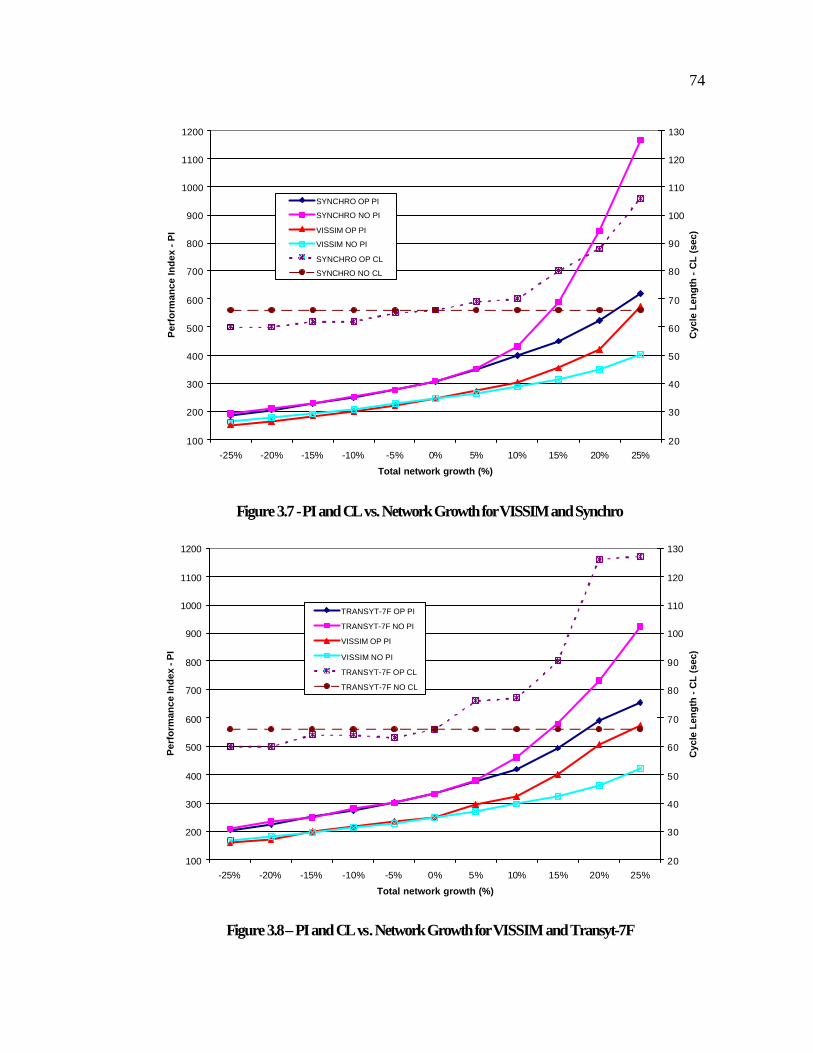
74
100
200
300
400
500
600
700
800
900
1000
1100
1200
-25% -20% -15% -10% -5% 0% 5% 10% 15% 20% 25%
Total network growth (%)
Per
form
ance
Ind
ex -
PI
20
30
40
50
60
70
80
90
100
110
120
130
Cyc
le L
eng
th -
CL
(se
c)
SYNCHRO OP PI
SYNCHRO NO PI
VISSIM OP PI
VISSIM NO PI
SYNCHRO OP CL
SYNCHRO NO CL
Figure 3.7 - PI and CL vs. Network Growth for VISSIM and Synchro
100
200
300
400
500
600
700
800
900
1000
1100
1200
-25% -20% -15% -10% -5% 0% 5% 10% 15% 20% 25%
Total network growth (%)
Per
form
ance
Ind
ex -
PI
20
30
40
50
60
70
80
90
100
110
120
130
Cyc
le L
eng
th -
CL
(se
c)
TRANSYT-7F OP PI
TRANSYT-7F NO PI
VISSIM OP PI
VISSIM NO PI
TRANSYT-7F OP CL
TRANSYT-7F NO CL
Figure 3.8 – PI and CL vs. Network Growth for VISSIM and Transyt-7F

75
100
200
300
400
500
600
700
800
900
1000
1100
1200
-25% -20% -15% -10% -5% 0% 5% 10% 15% 20% 25%
Total network growth (%)
Per
form
ance
Ind
ex -
PI
20
30
40
50
60
70
80
90
100
110
120
130
Cyc
le L
eng
th -
CL
(sec
)
SYNCHRO OP PI
SYNCHRO NO PI
SIMTRAFFIC OP PI
SIMTRAFFIC NO PI
SYNCHRO OP CL
SYNCHRO NO CL
Figure 3.9 - PI and CL vs. Network Growth for SimTraffic and Synchro
100
200
300
400
500
600
700
800
900
1000
1100
1200
-25% -20% -15% -10% -5% 0% 5% 10% 15% 20% 25%Total network growth (%)
Per
form
ance
Inde
x -
PI
20
30
40
50
60
70
80
90
100
110
120
130
Cyc
le L
engt
h -
CL
(sec
)
TRANSYT-7F OP PI
TRANSYT-7F NO PI
SIMTRAFFIC OP PI
SIMTRAFFIC NO PI
TRANSYT-7F OP CL
TRANSYT-7F NO CL
Figure 3.10 - PI and CL vs. Network Growth for SimTraffic and Transyt-7F

76
100
200
300
400
500
600
700
800
900
1000
1100
1200
-25% -20% -15% -10% -5% 0% 5% 10% 15% 20% 25%
Total network growth (%)
Per
form
ance
Ind
ex -
PI
20
30
40
50
60
70
80
90
100
110
120
130
Cyc
le L
eng
th -
CL
(sec
)
SYNCHRO OP PI
SYNCHRO NO PI
CORSIM OP PI
CORSIM NO PI
SYNCHRO OP CL
SYNCHRO NO CL
Figure 3.11 - PI and CL vs. Network Growth for Corsim and Synchro
100
200
300
400
500
600
700
800
900
1000
1100
1200
-25% -20% -15% -10% -5% 0% 5% 10% 15% 20% 25%
Total network growth (%)
Per
form
ance
Ind
ex -
PI
20
30
40
50
60
70
80
90
100
110
120
130
Cyc
le L
eng
th -
CL
(sec
)
TRANSYT-7F OP PI
TRANSYT-7F NO PI
CORSIM OP PI
CORSIM NO PI
TRANSYT-7F OP CL
TRANSYT-7F NO CL
Figure 3.12 - PI and CL vs. Network Growth for Corsim and Transyt-7F

77
The macroscopically obtained PIs from Figure 3.5 are similar. Both Synchro
and TRANSYT-7F OP timings yield lower PIs than the base NO timings. However,
the difference between OP and NO timings is much higher as demand grows.
There is a correlation between traffic demand and cycle length. This is because
the cycle length is a timing parameter that is used to increase throughput in the
network. When traffic demand increases, increasing the throughput is often the only
way to deal with congestion.
The results of the Direct CORSIM optimization are shown in Figure 3.6. The
optimal solutions are based on total delay (hours) because the PI is not available as an
objective function in the GA optimization. However, since total delay is a major
contributor of the PI, as defined in this study, it can be considered an equivalent
performance measure. For most of the scenarios, the signal timings optimized
through Direct CORSIM optimization do not yield lower PIs than the NO timings.
Figure 3.6 also shows that reported total delays for the OP timing plans (based on a
single simulation run) are lower than the average total delays obtained through 100
simulation runs with an OP timing plan.
The Figure 3.7 – Figure 3.12 show various trends in PIs for the microsimulation
tools. The OP and NO PI values represent averages from 10 simulation runs. In
general, VISSIM and CORSIM simulation tools do not justify use of the optimized
signal timings (NO timings are better). These microsimulation models, when used
with default parameters, report increased PIs for signal timings optimized by any of
the macroscopic tools. PIs from SimTraffic justify use of the optimized signal timings
from any of the two macroscopic optimization tools.

78
3.3.6.2 Uniform Changes in Traffic Distribution
Figures 3.13-3.20 show changes in PI impacted by the changes in turning
movement proportions. Both the left and right turning movement proportions were
changed at the same time. This approach had the opposite effect on the degree of
optimization. Increase in left turns is a limiting factor for the capacity of left turn
phases, which, if not satisfied, causes additional delays. At the same time, an increase
in right turns is a relaxing factor because the capacity of right turns is not limited due
to right-turns-on red. The proportion of through movement increases and the through
phase is under pressure when both turning movements decrease since the total traffic
demand is kept constant.
Each of the macro- and microsimulation outputs are presented for OP and NO
signal timings for all 10 scenarios. Figure 3.13 compares the PI changes for Synchro
and TRANSYT-7F. The PIs from both optimization tools show that they can find
better OP timings than the base NO timings. For the NO timing plans, TRANSYT-7F
better handles increases in through movements (turning movements are reduced) than
Synchro 6. However, when turning movements increase, Synchro 6 yields lower PIs
than TRANSYT-7F. The only case where the OP PI is not lower than the NO PI is for
the 20% decrease in turning proportions with TRANSYT-7F. For this scenario,
TRANSYT-7F’s PI (excessive fuel consumption) is minimal, although the PI used in
the study (Delays + 10 x Stops) is not. This inconsistency is the reason for the
discrepancy in microsimulation outputs based on TRANSYT-7F optimized signal
timings for this scenario.
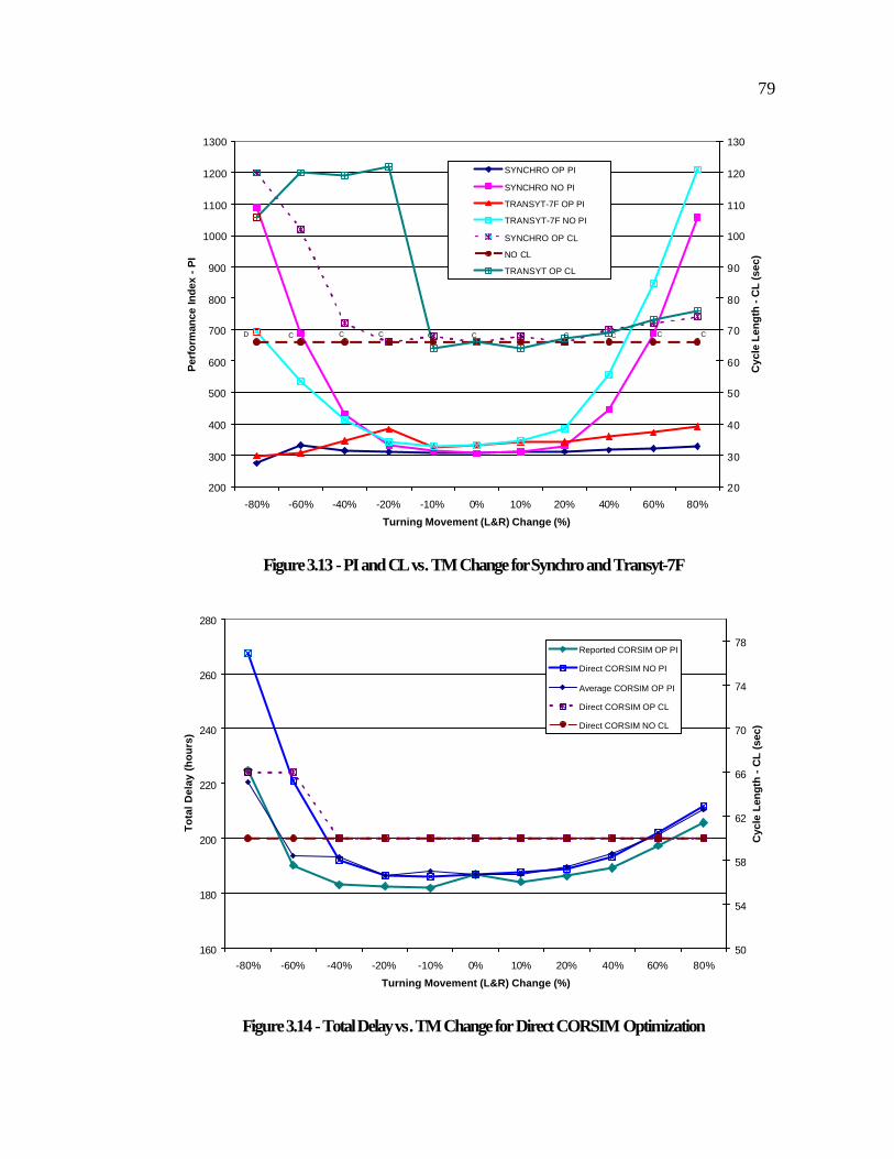
79
200
300
400
500
600
700
800
900
1000
1100
1200
1300
-80% -60% -40% -20% -10% 0% 10% 20% 40% 60% 80%
Turning Movement (L&R) Change (%)
Per
form
ance
Inde
x -
PI
20
30
40
50
60
70
80
90
100
110
120
130
Cyc
le L
eng
th -
CL
(sec
)
SYNCHRO OP PI
SYNCHRO NO PI
TRANSYT-7F OP PI
TRANSYT-7F NO PI
SYNCHRO OP CL
NO CL
TRANSYT OP CL
CD C C C CC C C C C
Figure 3.13 - PI and CL vs. TM Change for Synchro and Transyt-7F
160
180
200
220
240
260
280
-80% -60% -40% -20% -10% 0% 10% 20% 40% 60% 80%
Turning Movement (L&R) Change (%)
To
tal D
elay
(h
ou
rs)
50
54
58
62
66
70
74
78
Cyc
le L
engt
h -
CL
(sec
)
Reported CORSIM OP PI
Direct CORSIM NO PI
Average CORSIM OP PI
Direct CORSIM OP CL
Direct CORSIM NO CL
Figure 3.14 - Total Delay vs. TM Change for Direct CORSIM Optimization
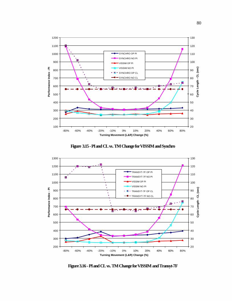
80
100
200
300
400
500
600
700
800
900
1000
1100
1200
-80% -60% -40% -20% -10% 0% 10% 20% 40% 60% 80%
Turning Movement (L&R) Change (%)
Per
form
ance
Ind
ex -
PI
20
30
40
50
60
70
80
90
100
110
120
130
Cyc
le L
eng
th -
CL
(se
c)
SYNCHRO OP PI
SYNCHRO NO PI
VISSIM OP PI
VISSIM NO PI
SYNCHRO OP CL
SYNCHRO NO CL
Figure 3.15 - PI and CL vs. TM Change for VISSIM and Synchro
200
300
400
500
600
700
800
900
1000
1100
1200
1300
-80% -60% -40% -20% -10% 0% 10% 20% 40% 60% 80%
Turning Movement (L&R) Change (%)
Per
form
ance
Inde
x -
PI
20
30
40
50
60
70
80
90
100
110
120
130
Cyc
le L
eng
th -
CL
(sec
)
TRANSYT-7F OP PI
TRANSYT-7F NO PI
VISSIM OP PI
VISSIM NO PI
TRANSYT-7F OP CL
TRANSYT-7F NO CL
Figure 3.16 - PI and CL vs. TM Change for VISSIM and Transyt-7F

81
200
300
400
500
600
700
800
900
1000
1100
1200
1300
1400
-80% -60% -40% -20% -10% 0% 10% 20% 40% 60% 80%Turning Movement (L&R) Change (%)
Per
form
ance
Inde
x -
PI
20
30
40
50
60
70
80
90
100
110
120
130
Cyc
le L
eng
th -
CL
(sec
)
SYNCHRO OP PI
SYNCHRO NO PI
SIMTRAFFIC OP PI
SIMTRAFFIC NO PI
SYNCHRO OP CL
SYNCHRO NO CL
Figure 3.17 - PI and CL vs. TM Change for SimTraffic and Synchro
200
300
400
500
600
700
800
900
1000
1100
1200
1300
1400
-80% -60% -40% -20% -10% 0% 10% 20% 40% 60% 80%
Turning Movement (L&R) Change (%)
Per
form
ance
Ind
ex -
PI
20
30
40
50
60
70
80
90
100
110
120
130
Cyc
le L
engt
h -
CL
(sec
)
TRANSYT-7F OP PI
TRANSYT-7F NO PI
SIMTRAFFIC OP PI
SIMTRAFFIC NO PI
TRANSYT-7F OP CL
TRANSYT-7F NO CL
Figure 3.18 - PI and CL vs. TM Change for SimTraffic and Transyt-7F

82
100
200
300
400
500
600
700
800
900
1000
1100
1200
-80% -60% -40% -20% -10% 0% 10% 20% 40% 60% 80%Turning Movement (L&R) Change (%)
Per
form
ance
Ind
ex -
PI
20
30
40
50
60
70
80
90
100
110
120
130
Cyc
le L
eng
th -
CL
(se
c)
SYNCHRO OP PI
SYNCHRO NO PI
CORSIM OP PI
CORSIM NO PI
SYNCHRO OP CL
SYNCHRO NO CL
Figure 3.19 - PI and CL vs. TM Change for CORSIM and Synchro
200
300
400
500
600
700
800
900
1000
1100
1200
1300
-80% -60% -40% -20% -10% 0% 10% 20% 40% 60% 80%Turning Movement (L&R) Change (%)
Per
form
ance
Inde
x -
PI
20
30
40
50
60
70
80
90
100
110
120
130
Cyc
le L
eng
th -
CL
(sec
)
TRANSYT-7F OP PI
TRANSYT-7F NO PI
CORSIM OP PI
CORSIM NO PI
TRANSYT-7F OP CL
TRANSYT-7F NO CL
Figure 3.20 - PI and CL vs. TM Change for CORSIM and Transyt-7F

83
Figure 3.14 shows the results for Direct CORSIM optimization timing plans for
changes in turning movements. The GA optimization procedure failed to produce
reliable OP timing plans. The reported optimized total delays are lower than the
averaged ones, showing the benefits of optimization where there are none. Except for
the scenarios of 80% and 60% decrease in turning movements, the average delays of
OP signal timings are not significantly different (at a 95% level of confidence) from
the NO delays.
The Figure 3.15 to Figure 3.20 show changes in PI from the microsimulation
outputs and macro optimization software used to optimize signal timings for the
simulation runs. Once again, the microsimulation tools behave quite differently. In
general, the PI results for each of the microsimulation tools are similar, regardless of
which macro optimization tool is used. Among the microsimulation tools, CORSIM
is the one that, when used with its default parameters, yielded to PIs that did not
justify use of the optimized signal timings. Results from VISSIM justified
optimization only when turning movements are increased. SimTraffic’s results
always justified the optimization. Use of an OP timing plan is justified when the
simulation PI generated by this plan is smaller than the simulation PI generated by
NO timing plans.
3.3.7 Discussion
The following paragraphs discuss the results of the evaluation of
macroscopically optimized timing plans in micro simulation tools.

84
3.3.7.1 Uniform Changes in Traffic Demand
PI results for OP timing plans from VISSIM (Figures 3.7 and 3.8) and
CORSIM (Figures 3.11 and 3.12) did not justify Synchro and TRANSYT-7F
optimizations when they were compared to NO timing plans. These findings are a
consequence of the fact that VISSIM and CORSIM have much higher vehicle
throughputs than those used by Synchro 6 or TRANSYT-7F in their analytical traffic
models. When demand increases, both Synchro 6 and TRANSYT-7F require an
increase in cycle length to increase throughput. However, the throughput is not
critical for the same link flows in VISSIM or CORSIM, so increasing cycle length is
unnecessary and increases delay. Therefore, the PI for OP signal timings is worse
than the PI for NO signal timings.
The differences between the capacities of SimTraffic, CORSIM, VISSIM and
the HCM method are described by Tian et al. (2002). A set of similar experiments is
conducted in this study for a single intersection approach to estimate the maximum
throughputs for all three types of simulation software. The results show that
maximum throughput rates for the three micro simulations are 0.52, 0.53, and 0.37
veh/sec/lane for VISSIM, CORSIM, and SimTraffic, respectively. For the sake of
comparison, the adjusted saturation flow rate from Synchro 6 (based on 1900
veh/hour/lane HCM ideal saturation flow rate) of 1770 veh/hour/lane is equivalent to
0.49 veh/sec/lane. These findings explain the behavior of VISSIM and CORSIM
outputs. They also explain why SimTraffic is sometimes more conservative than
macrosimulation tools (Figure 3.9 and 3.10).

85
Although throughput rate may be the most important reason for discrepancies
between macro- and microsimulations, it is not the only reason. Adjustment of
saturation flow rates in Synchro and TRANSYT-7F is tried in order to reduce the
discrepancies. The saturation flow rate in Synchro was adjusted to replicate
empirically measured VISSIM and CORSIM throughput rates. Although this action
reduced the optimal cycle length, the optimized timings still yielded a higher (worse)
PI than NO timings.
3.3.7.2 Uniform Changes in Traffic Distribution
The turning movement changes modeled in this study impact the cycle lengths
from the macro optimization in two ways. When turning proportions decrease,
optimized cycle length increases to provide enough capacity for a higher number of
through movements. Conversely, when turning proportions increase, the cycle length
maintains an almost constant value (with only a slight increase). The major benefits
of the OP timing plans in these cases come from optimizing phase splits.
When turning movement proportions decrease, through traffic at the
intersections increases. These cases are equivalent to an increase in traffic demand
only for the selected through movements. The explanation of the results in Figures
3.5-3.12 already shed some light on this problem. The throughput rates for VISSIM
and CORSIM are much higher than the adjusted saturated flow rates for Synchro and
TRANSYT-7F. Therefore, the increase in cycle length suggested by the macro
optimization tools is not justified for these two microsimulations. On the other hand,

86
the outputs for SimTraffic, whose throughput rate is lower, justify changes in cycle
lengths due to the increase in through demand.
The results are quite different among microsimulation tools for an increase in
turning movements. While SimTraffic and VISSIM outputs justify optimization of
signal timings, CORSIM does not. VISSIM results report lower benefits from the
optimization than Synchro or TRANSYT-7F. SimTraffic’s results in both cases show
higher benefits of optimization. Besides the differences in throughput rates for micro
simulations, these differences in results should also be associated with default lengths
of various vehicle types in each microsimulation.
It was observed that various microsimulations can handle different numbers of
vehicles for the same left turn storage lengths. For example, while SimTraffic and
VISSIM cannot handle more than 12 vehicles, CORSIM handles 14. For low turning
movements these differences are not essential. However, when left turn demand
approaches capacity, even one extra vehicle becomes critical. Since the traffic
demand is kept continuous throughout the analyzed peak hour, the oversaturated left
turn movements propagate queues and blockage of through lanes. This explains why
CORSIM simulation did not justify use of the optimized timing plans. Its left-turn
capacity was higher than those of other simulation tools.
3.3.7.3 Direct CORSIM Optimization
Although total delays (Figures 3.6 and 3.14) on optimized curves are either the
same or lower than nonoptimized delays, better timing plans could have been found if

87
more attention were given to Direct CORSIM optimization. There are three factors
that account for this.
First, it seems that 100 generations were not enough to reach optimal solution
for such a complex optimization. The timing plans might be better if the authors
divided the optimization process into a few steps, e.g., first optimizing the cycle
length, then optimizing splits and offsets (Hale 2005).
Second, in order to get the optimal solution, the initial solution should be as
close as possible to the sought optimal solution. This is a paradox of the Direct
CORSIM GA optimization. The optimization process is supposed to find the optimal
solution; it is not meant to be a procedure to fine-tune the optimal solution. The way
it is designed in the Direct CORSIM procedure, GA optimization becomes more of a
fine-tuning tool than a procedure for finding an optimal solution from a wide range of
possible solutions. Therefore, better signal timings may be found if the many signal
timing sets were tried as the initial points in the optimization procedure. However,
even if this were the case, there is no guarantee that a global optimum would have
been reached.
Third, even when TRANSYT-7F (Direct CORSIM optimization through
TRANSYT-7F) reported a better (than initial) solution, it is not always better when
the stochastic nature of microscopic simulation runs is considered. The TRANSYT-
7F manual (Hale 2005) does not explain the process of checking the quality of the
optimal solution. It seems that the performance of each timing plan is evaluated only
for one simulation run. The optimal timing plan is often slightly better than the
original timing plan. However, when the performance of the OP timing plan is

88
evaluated for many simulations runs (various random seeds), it may not be better than
the original timing plan. An illustration of this discrepancy can be seen in Figure 3.6
for the scenario of a 10% increase in traffic demand. In this case, the optimal solution
reported a decrease in delay for about ten hours while the average delay, obtained
from 100 runs, was higher than the delay for NO signal timings.
3.3.8 Summary of Selection of Appropriate Simulation Tools
The reliability of signal timing optimizations for two types of macroscopic
optimization software, Synchro and TRANSYT-7F 10, was evaluated in the three
most popular microsimulations in the U.S.: SimTraffic, CORSIM and VISSIM.
Default simulation parameters were used to perform the evaluations. In addition,
Direct CORSIM optimization, a new feature of the TRANSYT-7F software, was used
to perform a GA stochastic optimization within CORSIM. The following conclusions
are reached in this part of the study.
The results show that OP signal timings for various changes in traffic flows can
be justified in microsimulation software (SimTraffic). However, this justification
highly depends on the adjustments of the microsimulation parameters. It seems that
SimTraffic is calibrated in such a way to justify optimization schemes from
macroscopic optimization tools. The other two microsimulations need proper
calibration before they can be used for assessment of various signal timing plans.
However, the real question is whether macroscopic optimization and simulation
software can be adjusted to field-calibrated microsimulations. The answer to this

89
question will have to wait for the findings from the ageing of timing plans on real
world arterials.
The reliability of the stochastically optimized signal timings was evaluated
through hundreds of CORSIM runs. The GA optimization process is very slow and
highly dependant on the timing plan used as a starting point for the optimization.
Above all, the GA optimization generates timing plans that are not reliable when
evaluated through many CORSIM simulation runs. Except for a few extreme changes
in traffic flows, the results showed that for the examined traffic conditions, Direct
CORSIM optimization did not generate significantly better timing plans than the
existing plans. GA seems to be a powerful but unexplored optimization tool. If the
GA optimization is to be used as an everyday tool to optimize signal timings, more
guidance on how to use the optimization is needed. The areas where this procedure
lacks explanation are: design of the optimization process (multilevel versus all- in-
one), sensitivities of both parameters and results.
The findings from the evaluation of macroscopically optimized timing plans in
microscopic simulation tools can be summarized as:
• Only SimTraffic simulation is calibrated in such a way that justifies use of the
macroscopically developed optimized timing plans.
• Other microsimulation tools (VISSIM and CORSIM) need a comprehensive
calibration and validation of the underlying traffic models that are running
under these simulators.
• Calibration and validation of these microsimulators should be conducted with
a clear objective to justify use of the microscopically optimized timing plans.

90
Based on these results, Synchro and SimTraffic are selected to be used for
evaluating the deterioration of pretimed and actuated-coordinated control regimes.
However, SimTraffic simulation cannot be used for evaluating the deterioration of the
SCOOT adaptive control regime. This is because there is not an interface that
connects SCOOT and SimTraffic. For this reason, the deterioration of the SCOOT
control has to be done with VISSIM, the software that interfaces SCOOT. As
described in previous parts of this chapter, the method for determining the
deterioration of adaptive control relies on the deterioration of pretimed signals.
Therefore, VISSIM settings need to be calibrated in such a way to justify the use of
optimized timing plans from SYNCHRO. In short, a combination of Synchro and
SimTraffic tools is used to estimate the ageing of pretimed and actuated traffic
control while a combination of VISSIM, Synchro and SCOOT is used to estimate the
ageing of SCOOT adaptive control.
3.4 Major Modeling Process
Figure 3.21 shows a flowchart describing the modeling efforts for assessment
of deterioration of the three traffic control regimes. There were two aspects of
assessing the ageing of timing plans : deterministic and stochastic.
The deterministic aspect was described in the subsection of this chapter titled
“Traffic Demand and Distribution Scenarios.” Essentially, one base scenario and 20
various deterministic changes of traffic flows were modeled in Excel. Optimized
timing plans were then developed in Synchro for these traffic flows. Ten simulations
were run for both optimized and nonoptimized (base) timing plans. The whole
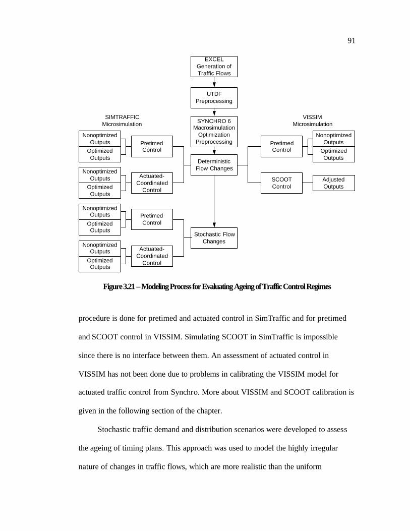
91
Actuated-Coordinated
Control
EXCELGeneration ofTraffic Flows
SYNCHRO 6Macrosimulation
OptimizationPreprocessing
PretimedControl
UTDFPreprocessing
PretimedControl
SCOOTControl
PretimedControl
NonoptimizedOutputs
OptimizedOutputs
AdjustedOutputs
NonoptimizedOutputs
OptimizedOutputs
NonoptimizedOutputs
OptimizedOutputs
NonoptimizedOutputs
OptimizedOutputs
SIMTRAFFICMicrosimulation
VISSIMMicrosimulation
DeterministicFlow Changes
Actuated-Coordinated
Control
NonoptimizedOutputs
OptimizedOutputs
Stochastic FlowChanges
Figure 3.21 – Modeling Process for Evaluating Ageing of Traffic Control Regimes
procedure is done for pretimed and actuated control in SimTraffic and for pretimed
and SCOOT control in VISSIM. Simulating SCOOT in SimTraffic is impossible
since there is no interface between them. An assessment of actuated control in
VISSIM has not been done due to problems in calibrating the VISSIM model for
actuated traffic control from Synchro. More about VISSIM and SCOOT calibration is
given in the following section of the chapter.
Stochastic traffic demand and distribution scenarios were developed to assess
the ageing of timing plans. This approach was used to model the highly irregular
nature of changes in traffic flows, which are more realistic than the uniform

92
deterministic changes applied in the first approach. For this purpose, 100 link flow
scenarios were generated in the Excel worksheet. Stochastic traffic demand was
modeled through Monte Carlo simulation with uniform distribution of network entry
input flows. Similarly, stochastic traffic distribution was modeled through Monte
Carlo simulation with uniform distribution of turning movement proportions.
However, unlike the deterministic scenarios, each entry point flow and turning
movement proportion was allowed to have a different value. Also differing from the
deterministic scenarios, the upper and lower limits were in percentages from the
mean values, ± 20% for entry input demand and ± 60% for turning movement
proportions. Uniform distribution was selected over normal distribution to model the
change of mean values and not around the mean value.
Stochastic experiments were done only for SimTraffic simulations. The reason
for this is the amount of computer time necessary to perform VISSIM simulations for
SCOOT control. SCOOT is a real-time traffic control system and its process of
optimizing signal timings cannot be speeded up. This obstacle prevents VISSIM from
running faster than real time. For 21 deterministic scenarios, it was necessary to
perform 210 VISSIM-SCOOT simulations. Considering that only one simulation can
be run at a time (only one SCOOT computer was available), it took 21 12-hour
working days to run these 210 simulations (10 1-hour simulations each day).
Stochastic simulations with SCOOT would require half the time and would not be
essential in determining the potential ageing of the SCOOT control.

93
3.5 Preparing VISSIM-SCOOT Simulations
The reliability of Synchro timing plans in SimTraffic has been checked. It was
found that the change in SimTraffic performance measures justify use of Synchro’s
optimizations. Simulation runs for the Synchro-SimTraffic combination could be run
without any further adjustments. However, before VISSIM simulations could be run,
it was important to calibrate VISSIM to support use of the optimized pretimed plans
from Synchro. In addition, SCOOT settings based on incoming traffic from VISSIM
had to be calibrated. The following subsections describe validation efforts for
VISSIM with pretimed control, the SCOOT-VISSIM connection, and validation of
SCOOT settings.
3.5.1 VISSIM Calibration for Pretimed Traffic Control
Data between Synchro and VISSIM are shared through the UTDF format.
Saving data from Synchro in the UTDF format is one of Synchro’s standard features.
Link traffic flows, signal phasing and timing data, network layout and lanes are
transferred by TEAPAC’s pre-processor “Pre-Synchro” from the UTDF files to
VISSIM. As a result, links, connectors and nodes are built in the VISSIM
environment. Traffic flows are converted into VISSIM’s traffic inputs and routing
decisions automatically. Also, signal timing and phasing data from Synchro are saved
as separate NEMA files for each signal in the network. In short, all basic data are
accurately transferred to VISSIM.
However, underlying car-following and driver behavior models in VISSIM are
not adjusted to Synchro’s model. It is a question of whether they can be properly

94
adjusted at all. Preliminary runs (described in previous sections of this chapter)
showed that the major problem is throughput. Throughput is largely influenced by
adjusted saturation flow rate at the intersections.
Saturation flow rate is one of the most important parameters in the field of
traffic control. Basically, this parameter represents a service rate at the queue channel
which, in this case, is an approach to the signalized intersection. By adjusting
saturation flow rate, we effectively adjust the service rate of the signal’s phase. When
signal timings are calibrated in the field, the values for this parameter are collected by
observing how many vehicles pass the stop line during a given green interval.
Saturation flow rate depends on driving habits of the local population, geometry of
the intersection, grade of the terrain, weather, pavement conditions, etc. The Highway
Capacity Manual (HCM) (HCM 2000) defines ideal saturation flow rates for certain
road types. These rates are then adjusted for the aforementioned factors to get actua l
saturation flow rates at the intersection approaches.
Synchro complies with the HCM and uses the same approach to calculate
adjusted saturation flow rates. Default VISSIM parameters are, however, set in such a
way that saturation flow rates measured from its simulations are much higher than
those from Synchro. As a consequence, “VISSIM’s traffic control,” with the same
parameters as “Synchro’s traffic control,” serves more vehicles in the same amount of
time.
This difference has a crucial impact when the optimization is performed. Since
it has smaller saturation flow rates, Synchro assumes that larger cycle lengths are
needed to increase vehicle throughput. It is well known (Tarnoff and Ordonez 2004)

95
that larger cycle lengths increase delays. Consequently, with optimized timings from
Synchro, additional cycle length and increase of delays is transferred to VISSIM.
VISSIM’s traffic, on the other hand, does not see any benefits from the longer cycle
length. Instead, it sees all the delays caused by the longer cycle length. For this
reason, VISSIM’s performance under optimized timing plans from Synchro is often
worse than with non-optimized plans. As a rule, these nonoptimized timing plans
usually have shorter cycle lengths.
VISSIM’s saturation flow rate can be changed by adjusting the parameters
Additive Part of Desired Safety Distance (BX_ADD) and Multiplicative Part of
Desired Safety Distance (BX_MULT) contained within the Wiedemann 74 car
Following Model (PTV AG 2005). The VISSIM Manual provides a lookup table that
lists saturation flow rate values for major combinations of BX_ADD and BX_MULT.
However, it is not possible to properly calibrate VISSIM by simply adjusting these
parameters to match Synchro's saturation flow rate from VISSIM’s lookup table. The
approach that gives results is comparison of PIs from VISSIM and Synchro. This
means adjusting BX_ADD and BX_MULT in such a way to make the PI from
VISSIM’s simulation output as close as possible to Synchro’s output (for base traffic
conditions). If these two PIs are similar, it is expected that total performance of traffic
models contained in these two simulation tools will be similar. This means that the
models would yield similar results for any traffic conditions. Table 3.2 provides
values for Delay, # of Stops, and # of vehicles that have exited network for various
values of BX_ADD and BX_MULT. The last column in Table 3.2 represents the
Sum of Squared Differences (SSD). The differences between Delay, Stops, and

96
Table 3.2 – Calibration of VISSIM Saturation Flow Coefficients
BX_ADD BX_MULT Delay (Hours) Stops Vehicles SSD 3 3.5 194.4 26810 11889 3687544 3 4 201.7 27060 11883 2789549 3 4.5 211.3 28167 11878 317219
3.2 4 213.5 28465 11841 71928 3.2 4.5 218.6 29152 11890 178255 3.3 3.9 216.4 29008 11862 77720 3.3 4 219.4 29675 11857 893612 3.3 4.1 218.5 29143 11862 170965 3.3 4.2 219.1 29149 11870 175723 3.4 3.8 214.6 27930 11874 640190 3.4 3.9 215.1 29017 11870 82611 3.4 4 222.2 29263 11854 284788 3.4 4.1 218.4 28639 11865 8580 3.4 4.2 224.7 30528 11851 3233650 3.5 3.5 213.4 28393 11857 114283 3.5 3.7 218.8 28929 11868 39812 3.5 3.8 217.5 28695 11881 1316 3.5 3.9 221 29208 11869 228641 3.5 4 219.9 29174 11873 197235 3.5 4.1 224 29858 11872 1272457 3.5 4.2 231.4 31449 11843 7394349 3.5 4.5 244.5 34418 11835 32355675 3.6 3.8 225.5 30634 11872 3625282 3.6 3.9 227.3 29817 11856 1182145 3.6 4 232.4 31284 11865 6523170 3.6 4.1 239.7 34966 11836 38889793 3.7 3.7 226.7 30264 11873 2353205 3.7 4.2 242.1 33098 11851 19080493 3.8 3.5 228.3 30515 11852 3187011 4 3.5 236.1 31987 11845 10609357 4 4 253.5 36249 11828 56538767 4 4.5 275.1 41396 11804 160435646
SYNCHRO 227 28730 11880 0

97
Vehicles values and corresponding Synchro values are taken, squared, and summed.
The minimal SSD means that VISSIM’s PI for corresponding BX_ADD and
BX_MULT is the closest to Synchro’s PI.
Therefore, the values 3.5 and 3.8 are chosen for BX_ADD and BX_MULT,
respectively. VISSIM’s results for pretimed traffic control, presented in the next
chapter, validate selection of these values.
3.5.2 SCOOT – VISSIM Connection
The SCOOT-VISSIM interface is developed to evaluate an integrated traffic
system including vehicle traffic, bus, rail transit, pedestrian and bicyclists controlled
by SCOOT in the VISSIM simulation environment. This section describes the major
elements and data flows of the SCOOT-VISSIM interface.
VISSIM consists of two parts: traffic simulator and signal state generator. The
former simulates traffic flow, while the latter determines signal phases and timings.
The traffic simulator sends detector values to the signal state generator each second.
Based on received detector data, the signal state generator determines optimal signal
timing parameters and sends them back to the traffic simulator. Figure 3.22 shows the
internal structure of VISSIM’s simulation system.
Signal Controller Junction (SCJ) defines the signal controller that controls the
signal phases of the junction (intersection) during the simulation. SCJ also allows the
external signal control system to supplement its own signal generator. This is done by
setting the optional Vehicle Actuated Programming (VAP) module to model detector-
based signal control. Each signal controller has its own individual VAP module. This

98
Iterationeach
Second
Detector Values
Traffic Simulation
Microscopic traffic flowmodel moving cars, trucks,LRT, buses andpedestrians in the network
Signal Values
Controller 1
Online Analysis
- Animation of vehicles- Vehicle data- Dynamic signal settings- Detector values- Travel times
Offline Analysis
- Travel times on segments- Delay at junctions- Queues at junctions- Cross section data- Time-space diagram- Acceleration statistics- Dynamic signal timing
Controller 2
Controller 3
Controller 12
Signal Control
VAP (VehicleActuated Phasing)models one SCATSSystem with same cyclelength at each controller
VISSIM Verkehr In Stadten - SIMulation (Traffic in Towns - Simulation)
Figure 3.22 - Internal Structure of VISSIM Simulation Software
characteristic makes SCOOT-VISSIM interface different from the Dynamic Link
Library (DLL) of the SCOOT-CORSIM interface (Hansen and Martin 1998). The
SCOOT-VISSIM interface includes two parts: the VAP modules for signa l
controllers, and the communication module, both developed in VISUAL C++ (Feng
and Martin 2003). The functions of the VAP module are:
• Get detector data from the SCJs
• Exchange virtual detector data and new SCOOT signal timings between the
SCJs and the communication module
• Implement new traffic signal lights

99
The functions of the communication module are:
• Exchange detector data between each VAP and SCOOT
• Retrieve new SCOOT signal timings
• Distribute SCOOT signal timings to the corresponding VAP
Every SCJ in the VISSIM network has one VAP module to control the
exchange. Figure 3.23 shows the architecture and data flow of the SCOOT-VISSIM
simulation environment.
3.5.3 SCOOT Validation
SCOOT’s working principles were described in the previous chapter. Basically,
the quality of SCOOT’s performance is mostly affected by its ability to model
arrivals and service rate at each intersection approach. If these two variables are
known, SCOOT can be adjusted to perform efficiently.
The arrival of vehicles at a stop bar is estimated by the SCOOT traffic model.
This model estimates when vehicles detected upstream will arrive at the stop bar. The
model takes into account the journey time necessary to travel from the detectors to
the stop bar and dispersion of the vehicles in the platoon. SCOOT does not allow
adjustment of the platoon dispersion model. The only parameter that can be changed
to adjust the accuracy of vehicle arrivals is Journey Time – JNYT.
Service rate at the signal approach is represented by saturation flow rate or
SCOOT’s equivalent saturation occupancy. This parameter is the most important
parameter for SCOOT validation. It impacts both the platoon of vehicles that will
depart from the approach, as well as the number of vehicles that will potentially

100
SCOOT 4.2
COMMUNICATIONMODULE
...... ......VAP MODULE 1 VAP MODULE i VAP MODULE n
SCJ i......
SIGNAL STATE GENERATOR
......
VISSIM
Virt
ual D
etec
tor S
tatu
s an
dS
igna
l Pha
ses
of th
e W
hole
Net
wor
kN
ew S
CO
OT
Signal P
hasesof the W
hole Netw
ork
TRAFFIC SIMULATOR
SCOOT-VISSIMINTERFACE
TCP/IP
DDE
DDE
Alphastation 255/300OpenVMS 7.1
Pentium 4 2.8 GHzWindows XP
SCOOT SYSTEM
VAP: Vehicle Actuated ProgrammingSCJ: Signal Controller JunctionDDE: Dynamic Data ExchangeTCP/IP: Transmission Control Protocol / Internet Protocol
Virtual Detector Status and Signal Phase of the Corresponding Controller
New SCOOT Signal Phase of the Corresponding Controller
SCJ 1 SCJ n
Figure 3.23 – VISSIM-SCOOT Simulation Environment

101
remain in the queue. Saturation Occupancy - STOC is a SCOOT parameter that is
used to adjust this service rate.
There are a few other parameters important for SCOOT validation. Start Lag
Time (SLAG) represents the time from the appearance of green on the street to the
time when the traffic queue effectively starts moving. Similarly, End Lag Time
(ELAG) is the time from the appearance of amber on the street to the time of
effective cessation of traffic movements. Maximum queue clear time (QCMQ)
represents the time necessary for the maximum traffic queue to clear the intersection.
This parameter helps SCOOT to recognize when traffic queues are causing
congestion upstream of the detectors.
All of these parameters help traffic engineers to adjust SCOOT to best
represent real traffic conditions. If, for example, the STOC is too small or the JNYT
is too short, SCOOT’s model will estimate vehicles in queue when there are none.
Similarly, if the STOC is too high or the JNYT is too long, SCOOT’s model will not
be able to estimate vehicles in queue when they are there.
Validation of SCOOT is the process in which vehicle estimates from SCOOT’s
models are compared with real-world vehicles. This process follows calibration of
SCOOT parameters in which all of the aforementioned parameters are adjusted.
SCOOT validation in this study was done by comparing the number of vehicles in
queue from the SCOOT model with the number of vehicles in queue from the traffic
simulation. Traffic simulation here plays the role of real-world traffic conditions.
Figure 3.24 shows screenshots from both SCOOT and VISSIM. The upper part
of Figure 3.24 shows SCOOT’s link validation facility, which reports the number of
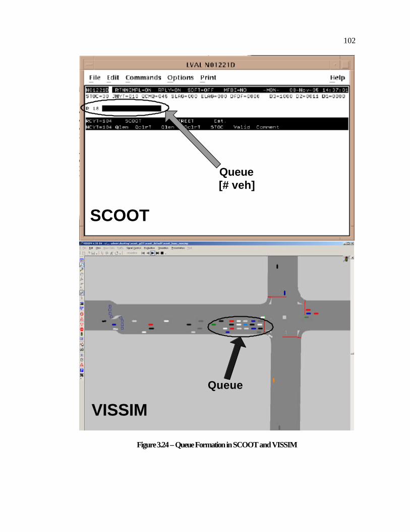
102
SCOOT
VISSIM
Queue[# veh]
Queue
Figure 3.24 – Queue Formation in SCOOT and VISSIM
103
vehicles in queue. The black bar in the upper left corner varies as vehicles join or
leave the queue. R stands for red light and the number 18 represents the current
number of vehicles in queue. The lower part of the figure shows queue formation at
an intersection approach from VISSIM. At the time instance shown in Figure 3.24,
the number of vehicles in queue from VISSIM (16 vehicles standing and two just
about to join the queue) closely matches SCOOT’s queue estimation.
Figure 3.25 shows the coefficient of determination between queues in SCOOT
and VISSIM at the end of the red light intervals. The data consists of parallel queue
measures taken at the two busiest approaches for each of the nine intersections in the
network. Traffic conditions during the data collection were the same as for the base
scenario in modeling the deterioration of traffic control regimes. The coefficient of
determination (R2) shows that there is a high correlation between number of vehicles
in queue for SCOOT and VISSIM. An underlying least square model shows that
SCOOT estimates around 18 vehicles when 20 vehicles are standing in real queue.
The results of the validation show that, in general, SCOOT has been validated
properly.
The SCOOT estimation error is most likely result of imperfections in modeling
the dispersion of the traffic platoon and imperfections in converting the SCOOT’s
LPUs into the actual number of vehicles. A coefficient of determination of 0.84 is
pretty high. The results from real-world SCOOT installations rarely have such high
correlations between real queues and queues from the SCOOT model (Jayakrishnan
et al. 2001).

104
y = 1.0234x + 1.2714R2 = 0.8396
0
5
10
15
20
25
30
0 5 10 15 20 25 30
SCOOT Queue [veh]
VIS
SIM
Que
ue [v
eh]
Figure 3.25 – Correlation between Traffic Queues in SCOOT and VISSIM
3.6 Summary of Research Methodology
The first part of this chapter defined ageing (deterioration) of traffic control
regimes. It is important to understand that ageing in this study means the process of
deterioration of a traffic control regime due to long and steady changes in underlying
traffic conditions (demand and distribution). All common cyclical (diurnal and
weekly) traffic fluctuations and variations are not considered by this approach.
A method is proposed to measure the extent of the signal timing plans’ ageing.
This method relies on the existence of optimized pretimed traffic plans for any
experienced change in traffic flows. Existence of these plans is a crucial factor in
determining ageing of adaptive traffic controls.

105
The second part of the chapter discussed design of simulation experiments. An
arterial network with basic features of modeled traffic controls are introduced in this
section. A scenario of base traffic conditions is presented, along with 20 other
scenarios for various traffic demands and distributions. Experiments with these
variations were done both for selection of appropriate simulation tools and
assessment of deterioration of traffic control regimes.
The third part of the chapter is very important. It describes efforts to select
proper simulation tools for assessing the deterioration of traffic control regimes.
Thousands of simulations are performed to find the best combination of macro- and
microsimulation tools. Finally, the results showed that Synchro-SimTraffic is the best
combination. However, it was also concluded that VISSIM simulation has to be
calibrated for pretimed traffic control. VISSIM is the only simulator that is connected
to SCOOT and that can be used to assess the ageing of the SCOOT control.
The fourth part of the chapter describes the major modeling process. Pretimed
and actuated controls are modeled (using the Synchro-SimTraffic combination) for
both deterministic and stochastic changes in traffic flows. Pretimed and SCOOT
adaptive controls are modeled only for deterministic changes in traffic flows.
The last part of the chapter describes tasks for preparing for the VISSIM and
SCOOT simulations. First, VISSIM is calibrated in such a way to justify use of
optimized timing plans from Synchro. The basic features of VISSIM- SCOOT
connection are then presented. Finally, SCOOT validation is performed. The results
confirmed that SCOOT settings are fairly calibrated to represent ‘real’ conditions
from the VISSIM simulation.

CHAPTER 4
RESULTS
This chapter presents the results of the modeling. The results are presented in
the form of graphs and tables with minimal discussion of their meanings. A major
discussion of the findings is given in the next chapter. The chapter is divided into four
sections. The first part of the chapter presents a general finding about the
methodology used in this study. The second section deals with the reliability of the
ageing measure used in Bell’s work (Bell 1985). The third part of the chapter presents
the results for ageing of pretimed and actuated-coordinated traffic control regimes for
deterministic and stochastic changes in traffic flows. The final part of the chapter
shows the results of assessing the ageing of SCOOT adaptive control.
4.1 Justification of the Adopted Approach for Measuring Ageing
Figure 4.1 shows the relationship between the PI and uniform increase in traffic
demand over the entire network. The purpose of Figure 4.1 is to validate the assumed
idealized concept of ageing shown in Figure 3.1. The findings show almost no
difference in PI for optimized and non optimized traffic control for a 5% increase in
traffic demand. As traffic demand grows, the difference in PI becomes greater.

107
0
200
400
600
800
1000
1200
0 5 10 15 20 25
Increase in Traffic Demand [%]
Per
form
ance
In
dex
Non Optimized
Optimized
Figure 4.1 - Modeled Impact of the Uniform Increase in Traffic Demand on PI
4.2 Reliability of Bell’s Ageing Measure
Figures 4.2 – 4.5 show the relationship between the benefits of updating signal
timings and CF – Average Absolute Difference in Link Flows. The figures show this
relationship for a pretimed traffic control regime for four different types of changes in
link flows. The CF parameter is calculated using Equation [2.1]. The benefits of
updating signal timings are calculated according to Equation [3.1]. Figures 4.2-4.5
show a high coefficient of determination (R2) between the CF parameter and the
benefits of updating signal timing plans.

108
TRAFFIC DEMAND DECREASED
-3
-2
-1
0
1
2
3
4
5
6
7
8
20 40 60 80 100 120
CF - Average Absolute Difference in Link Flow (veh)
Ben
efit
of
Up
dat
ing
Sig
nal
Tim
ing
s (%
) -25%-20%-15%-10%-5%Base
R2=0.794
Outliers
Figure 4.2 - Benefits of Updating vs CF for Decreased Traffic Demand
TRAFFIC DEMAND INCREASED
-10
-5
0
5
10
15
20
25
30
35
20 30 40 50 60 70
CF - Average Absolute Difference in Link Flow (veh)
Ben
efit
of
Up
dat
ing
Sig
nal
Tim
ing
s (%
) Base5%10%15%20%25%
R2=0.80
Figure 4.3 - Benefits of Updating vs CF for Increased Traffic Demand

109
TURNING MOVEMENTS DECREASED
-10
0
10
20
30
40
50
60
20 40 60 80 100 120
CF - Average Absolute Difference in Link Flow
Ben
efit
of
Up
dat
ing
Sig
nal
Tim
ing
s (%
)
-80%-60%-40%-20%-10%Base
R2=0.895
Figure 4.4 - Benefits of Updating vs CF for Decreased Turning Movements
TURNING MOVEMENTS INCREASED
-10
0
10
20
30
40
50
60
70
80
20 40 60 80 100 120 140
CF- Average Absolute Difference in Link Flow (veh)
Ben
efit
of U
pd
atin
g S
ign
al T
imin
gs
(%)
Base10%20%40%60%80%
R2=0.94
Figure 4.5 - Benefits of Updating vs CF for Increased Turning Movements

110
Figure 4.2 shows how the benefits of updating timing plans are related to a
decrease in traffic demand. For an average decrease of 20 vehicles per link, around
2% of delay and stops could be saved by retiming traffic signal timing plans.
Figure 4.3 shows the impact of the increase in traffic demand on the benefits of
updating signal timings. The figure shows that the benefits increase up to a certain
point. On the section where benefits increase, around 10% benefits are estimated fo r
an average increase of 10 vehicles per link.
Figure 4.4 shows the relationship between the benefits of updating and the
decrease in turning movement proportions. A decrease in turning movements (and
increase in through movements) equivalent to the CF ageing measure of 10 yield
around a 5% increase in benefits of retiming traffic signal timing plans. The results
show that the benefits could reach 50%.
The relationship between the benefits of updating signal timings and the
uniform increase in turning movements is shown in Figure 4.5. An increase in turning
movements (and decrease in through movements) equivalent to the CF ageing
measure of 10 yields around a 10% increase in the benefits of retiming traffic signal
timing plans. The results show that the benefits of updating can be as high as 75%.
Figure 4.6 shows the same relationship between the benefits of updating and
the average change in network traffic demand. The average change in network traffic
demand represents a measure used to express random changes in traffic demand and
turning movements which occur at each link, independently of other links (traffic
flows are still balanced). In other words, Figure 4.6 represents all of the changes
randomly applied in the network from the previous four figures. Unlike Figures 4.2 –

111
0
10
20
30
40
50
60
-10 -5 0 5 10Average Change in Network Traffic Demand (%)
Ben
efit
s o
f Up
dat
ing
Sig
nal
Tim
ing
s (%
)
CF<= 50
50 < CF < 55
CF => 55
R2=0.01
Figure 4.6 - Benefits of Updating Timings vs Average Change in Traffic Demand
4.5, Figure 4.6 shows no correlation between the benefits of signal timings and the
CF measure.
4.3 Ageing of Pretimed and Actuated Traffic Controls
This section is divided into two parts. The first part deals with changes in traffic
control performance as a result of deterministic changes in traffic demand and
distribution. The second subsection deals with stochastic or random changes and their
impact on traffic control.
4.3.1 Deterministic Traffic Demand and Distribution Inputs
The first part of this section show the performances of optimized and non-
optimized timing plans for various changes in traffic flows. Figure 4.7 shows the

112
100.00
300.00
500.00
700.00
900.00
1100.00
1300.00
-25% -20% -15% -10% -5% 0% 5% 10% 15% 20% 25%
Total Network Growth (%)
Per
form
ance
Inde
x -
PI
SIM TRAFFIC UPPER OPTSIM TRAFFIC OPTSIM TRAFFIC LOWER OPTSIM TRAFFIC UPPER NOSIM TRAFFIC NOSIM TRAFFIC LOWER NO
Figure 4.7 – PI vs Total Network Growth for Pretimed Traffic Control
performance index of optimized and nonoptimized timing plans for scenarios
representing various levels of traffic demand. For most of the scenarios, optimized
timing plans generate smaller a PI (fewer delays and stops) than nonoptimized timing
plans. The difference between plans is more accentuated for an increase in traffic
demand.
Figure 4.8 shows the performance of optimized and nonoptimized timing plans
for scenarios representing various proportions of turning movements at intersection
approaches. Optimized timing plans are better (smaller PIs) than nonoptimized timing
plans for almost all scenarios. The only exception is a 10% reduction in turning
movements where optimized and nonoptimized timings do not yield to statistically
different PIs.

113
200.00
400.00
600.00
800.00
1000.00
1200.00
1400.00
1600.00
-80% -60% -40% -20% -10% 0% 10% 20% 40% 60% 80%
Turning Movement (L&R) Change (%)
Per
form
ance
Inde
x - P
I
SIM TRAFFIC UPPER OPTSIM TRAFFIC OPTSIM TRAFFIC LOWER OPTSIM TRAFFIC UPPER NOSIM TRAFFIC NOSIM TRAFFIC LOWER NO
Figure 4.8 - PI vs Change in Turning Movements for Pretimed Traffic Control
Figures 4.9 and 4.10 show the performances of optimized and nonoptimized
timing plans for actuated-coordinated traffic control. Figure 4.9 shows the PI’s
dependence on changes in traffic demand. Much like the results for pretimed traffic
control, these results prove the supremacy of optimized plans over nonoptimized
plans. The optimized timing plans are not better only for scenarios with a ± 5%
change in traffic demand (Table 4.3). In these cases, changes in traffic volumes are so
small that they canno t impact the performance of nonoptimized timing plans.
Figure 4.10 shows that optimized timing plans are not better than non-
optimized plans for all scenarios where turning movement proportions are reduced.
This inconsistency does not come from the fact that optimized timing plans do not

114
100.00
200.00
300.00
400.00
500.00
600.00
700.00
800.00
900.00
1000.00
1100.00
-25% -20% -15% -10% -5% 0% 5% 10% 15% 20% 25%
Total Network Growth (%)
Per
form
ance
Inde
x -
PI
SIM TRAFFIC UPPER OPTSIM TRAFFIC OPTSIM TRAFFIC LOWER OPTSIM TRAFFIC UPPER NOSIM TRAFFIC NOSIM TRAFFIC LOWER NO
Figure 4.9 - PI vs Total Network Growth for Actuated Traffic Control
100.00
200.00
300.00
400.00
500.00
600.00
700.00
800.00
900.00
1000.00
1100.00
-80% -60% -40% -20% -10% 0% 10% 20% 40% 60% 80%
Turning Movement (L&R) Change (%)
Per
form
ance
Inde
x -
PI
SIM TRAFFIC UPPER OPTSIM TRAFFIC OPTSIM TRAFFIC LOWER OPTSIM TRAFFIC UPPER NOSIM TRAFFIC NOSIM TRAFFIC LOWER NO
Figure 4.10 - PI vs Change in Turning Movements for Actuated Traffic Control

115
work well. It comes from the fact that nonoptimized timing plans for actuated control
can perform very well for these scenarios.
Statistical testing is necessary to investigate the validity of the differences
between optimized and nonoptimized plans. For this purpose, hypothesis tests about
the difference between the means of two populations with independent samples are
used. Two populations represent all possible PI values from simulation runs for non-
optimized (first population) and optimized (second population) signal timing plans.
The objective is to test whether the mean of the PIs from the nonoptimized simulation
runs is higher than the mean of the PIs from optimized simulation runs.
We set up the null hypothesis mathematically as:
H0: µ1 - µ2 = 0 [4.1]
With an alternative hypothesis as:
Ha: µ1 - µ2 > 0 [4.2]
Where
µ1 – Mean PI for population of non-optimized PIs
µ2 – Mean PI for population of optimized PIs
The tests statistic for the small-sample case (n1 = n2 = 10) is:
+
−−−=
21
2
2121
11
)()(
nns
xxt
µµ [4.3]
Where:
x1 – Mean PI for sample from population of non-optimized PIs
x2 – Mean PI for sample from population of optimized PIs

116
s2 – Estimate of common variance σ2
In the case of two independent random samples of sizes n1 and n2, the t
distribution will have degrees of freedom:
221 −+= nndf [4.4]
However, the variances of the two populations are not equal (σ12 ≠ σ2
2). If we
assume that the populations are normally distributed (which is mostly true), we
estimate the standard deviation of the sampling distribution (sx1-x2 - estimate of σx1 -
σx2) as:
2
22
1
21
21 ns
ns
sxx
+=−
[4.5]
In this case, the t distribution is still used but with degrees of freedom
calculated as:
)]1(/)/[()]1(/1[]/)/(/1[
222
221
221
21
22
21
221
−+−+
=nnssnn
nssndf [4.6]
Where:
n1 – sample size of the first population (population consists of PIs for non-
optimized signal timings)
n2 – sample size of the second population (population consists of PIs for
optimized signal timings)
Tables 4.1- 4.4 show the results of hypothesis testing for pretimed traffic
control and changes in traffic demand for a 95% level of confidence. The results
show that nonoptimized signal timings are greater than optimized for most traffic
demand scenarios. If traffic demand changes by ± 5%, this change will not have a

117
Table 4.1 – Testing for Pretimed SimTraffic Control – Traffic Demand
Scenario Control Mean PI St. Dev S12 Tstatistic Df Ttable H0 NO 168.87 2.76
-25% OP 168.88 3.08
1.31 -0.03 17.78 1.73 UPHOLD
NO 200.62 5.00 -20%
OP 187.70 5.40 2.33 18.93 17.89 1.73 REJECT
NO 221.00 4.83 -15%
OP 214.01 2.51 1.72 11.93 13.54 1.76 REJECT
NO 240.79 5.35 -10%
OP 238.89 5.21 2.36 2.75 17.99 1.73 REJECT
NO 273.47 7.52 -5%
OP 272.58 6.97 3.24 1.10 17.90 1.73 UPHOLD
Base NO 305.37 10.07 NO 384.88 39.51
5% OP 387.89 31.84
16.05 -1.68 17.22 1.74 UPHOLD
NO 486.89 52.60 10%
OP 458.87 30.63 19.25 14.28 14.48 1.75 REJECT
NO 630.39 63.18 15%
OP 507.81 40.69 23.76 56.23 15.37 1.75 REJECT
NO 817.20 83.19 20%
OP 623.47 61.03 32.63 75.84 16.51 1.74 REJECT
NO 1022.98 72.23 25%
OP 841.79 64.37 30.60 73.25 17.77 1.73 REJECT

118
Table 4.2 – Testing for Pretimed SimTraffic Control – Traffic Distribution
Scenario Control Mean PI St. Dev S12 Tstatistic Df Ttable H0 NO 616.91 51.59
-80% OP 336.46 6.22
16.43 154.70 9.26 1.83 REJECT
NO 490.38 66.85 -60%
OP 355.94 6.93 21.25 65.20 9.19 1.83 REJECT
NO 385.97 20.86 -40%
OP 293.94 7.38 7.00 77.81 11.22 1.80 REJECT
NO 330.50 18.58 -20%
OP 304.29 16.20 7.79 20.99 17.67 1.73 REJECT
NO 314.70 10.76 -10%
OP 307.56 7.40 4.13 7.86 15.96 1.75 REJECT
Base NO 305.37 10.07 NO 316.01 9.79
10% OP 318.01 7.56
3.91 -2.26 16.92 1.74 UPHOLD
NO 369.08 27.77 20%
OP 329.20 20.35 10.89 27.03 16.50 1.74 REJECT
NO 566.37 57.01 40%
OP 345.57 16.17 18.74 114.06 10.44 1.81 REJECT
NO 926.37 96.07 60%
OP 352.44 9.69 30.53 232.25 9.18 1.83 REJECT
NO 1361.55 131.23 80%
OP 376.94 16.37 41.82 340.45 9.28 1.83 REJECT

119
Table 4.3 – Testing for Actuated SimTraffic Control – Traffic Demand
Scenario Control Mean PI St. Dev S12 Tstatistic Df Ttable H0 NO 181.42 3.19
-25% OP 171.58 2.85
1.35 18.92 17.78 1.73 REJECT
NO 199.24 6.15 -20%
OP 192.84 5.31 2.57 8.92 17.63 1.73 REJECT
NO 218.52 5.68 -15%
OP 211.80 5.05 2.40 9.69 17.76 1.73 REJECT
NO 240.87 5.00 -10%
OP 228.74 4.37 2.10 18.72 17.68 1.73 REJECT
NO 266.23 6.62 -5%
OP 265.99 6.00 2.82 0.32 17.83 1.73 UPHOLD
Base NO 294.29 6.81 NO 354.09 27.90
5% OP 353.65 13.68
9.83 0.32 13.09 1.77 UPHOLD
NO 427.70 37.52 10%
OP 402.64 23.72 14.04 14.96 15.20 1.75 REJECT
NO 548.24 37.40 15%
OP 470.39 27.29 14.64 45.49 16.47 1.75 REJECT
NO 701.12 65.40 20%
OP 579.47 47.61 25.58 53.78 16.45 1.75 REJECT
NO 901.02 66.93 25%
OP 725.89 58.93 28.20 73.74 17.72 1.73 REJECT

120
Table 4.4 – Testing for Actuated SimTraffic Control – Traffic Distribution
Scenario Control Mean PI St. Dev S12 Tstatistic Df Ttable H0 NO 248.55 9.24
-80% OP 253.24 10.22
4.36 -5.03 17.82 1.73 UPHOLD
NO 281.44 16.63 -60%
OP 294.27 16.18 7.34 -10.59 17.99 1.73 UPHOLD
NO 282.65 9.74 -40%
OP 283.44 10.52 4.54 -0.82 17.89 1.73 UPHOLD
NO 290.28 8.77 -20%
OP 288.79 11.11 4.48 1.58 17.08 1.74 UPHOLD
NO 293.32 7.76 -10%
OP 292.91 8.00 3.52 0.49 17.98 1.73 UPHOLD
Base NO 294.29 6.81 NO 308.33 8.82
10% OP 301.39 5.36
3.26 8.59 14.85 1.75 REJECT
NO 347.41 22.72 20%
OP 315.82 14.35 8.50 24.23 15.20 1.75 REJECT
NO 468.29 55.52 40%
OP 327.84 12.66 18.01 74.01 9.93 1.81 REJECT
NO 682.20 84.91 60%
OP 343.76 5.25 26.90 145.90 9.07 1.83 REJECT
NO 953.07 62.42 80%
OP 368.61 10.28 20.01 292.19 9.49 1.83 REJECT

121
significant impact on the performance of the traffic control. This is also the case for
low levels of traffic demand (-25%). In this case, traffic volumes are so low that the
benefits of retiming signals are negligible.
Figures 4.11 – 4.14 show the relationship between the benefits of updating
timing plans and four different types of changes in link flows for pretimed and
actuated-coordinated control regimes. These benefits are calculated according to
Equation [3.1].
Figure 4.11 shows how the benefits of updating timing plans are related to a
decrease in traffic demand. The benefits are higher for actuated traffic control than
for pretimed control. For both of these control regimes, one could save around 2% in
delay and stops by retiming traffic signals for every 10% decrease in traffic demand.
Figure 4.12 shows the impact of the increase in traffic demand on the benefits of
y = 0.197x + 0.3344R
2 = 0.4904
y = 0.1184x + 0.2992R
2 = 0.1641
-4
-2
0
2
4
6
8
0 5 10 15 20 25
Decrease in Traffic Demand (%)
Ben
efit
of
Up
dat
ing
Sig
nal
Tim
ing
s (%
) Pre-Timed
Actuated
Linear (Actuated)
Linear (Pre-Timed)
Figure 4.11 - Benefits of Updating Timings vs Decrease in Traffic Demand

122
y = 0.9042x - 1.9679R2 = 0.7553
y = 1.0056x - 1.7627R2 = 0.6963
-20
-10
0
10
20
30
40
0 5 10 15 20 25
Increase in Traffic Demand (%)
Ben
efit
of
Up
dat
ing
Sig
nal
Tim
ing
s (%
) Pre-Timed
Actuated
Linear (Actuated)
Linear (Pre-Timed)
Figure 4.12 - Benefits of Updating Timings vs Increase in Traffic Demand
y = -0.0454x + 0.5307R2 = 0.1186
y = 0.554x - 1.8552R2 = 0.8957
-20
-10
0
10
20
30
40
50
60
0 10 20 30 40 50 60 70 80
Decrease in Turning Movements (%)
Ben
efit
of
Up
dat
ing
Sig
nal
Tim
ing
s (%
)
Pre-Timed
Actuated
Linear (Actuated)
Linear (Pre-Timed)
Figure 4.13 - Benefits of Updating Timings vs Decrease in Turning Movements
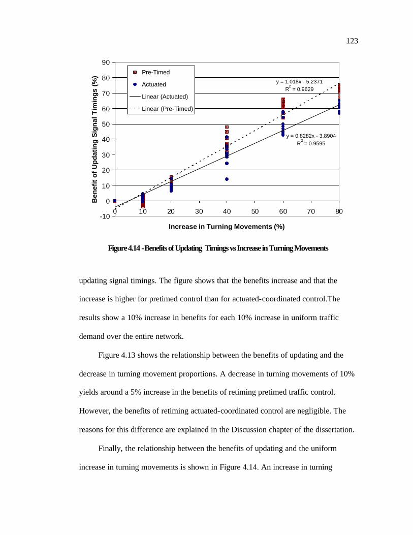
123
y = 0.8282x - 3.8904R
2 = 0.9595
y = 1.018x - 5.2371R
2 = 0.9629
-10
0
10
20
30
40
50
60
70
80
90
0 10 20 30 40 50 60 70 80
Increase in Turning Movements (%)
Ben
efit
of
Up
dat
ing
Sig
nal
Tim
ing
s (%
) Pre-Timed
Actuated
Linear (Actuated)
Linear (Pre-Timed)
Figure 4.14 - Benefits of Updating Timings vs Increase in Turning Movements
updating signal timings. The figure shows that the benefits increase and that the
increase is higher for pretimed control than for actuated-coordinated control.The
results show a 10% increase in benefits for each 10% increase in uniform traffic
demand over the entire network.
Figure 4.13 shows the relationship between the benefits of updating and the
decrease in turning movement proportions. A decrease in turning movements of 10%
yields around a 5% increase in the benefits of retiming pretimed traffic control.
However, the benefits of retiming actuated-coordinated control are negligible. The
reasons for this difference are explained in the Discussion chapter of the dissertation.
Finally, the relationship between the benefits of updating and the uniform
increase in turning movements is shown in Figure 4.14. An increase in turning

124
movements of 10% yields around an 8% increase in the benefits of retiming traffic
signals. The results show that the benefits of updating can be as high as 75%. The
benefits obtained after updating pretimed control are again higher than those of
actuated-coordinated control.
4.3.2 Stochastic Traffic Demand and Distribution Inputs
Figure 4.15 shows the results from the experiments with stochastic changes both in
traffic demand and turning movements. The results from the stochastic experiments
have shown that, regardless of the average change in network traffic demand, there is
an average benefit of 35% in terms of delay and number of stops from updating
pretimed signal timing plans. Similarly, the average benefit of retiming actuated-
coordinated signal timing plans is around 27%.
y = -0.3492x + 27.121R2 = 0.009
y = -0.7069x + 34.61R2 = 0.0434
-10
0
10
20
30
40
50
60
-10 -5 0 5 10
Average Change in Network Traffic Demand (%)
Ben
efit
s o
f Up
dat
ing
Sig
nal
Tim
ing
s (%
)
Actuated-Coordinated Pre-TimedLinear (Actuated-Coordinated) Linear (Pre-Timed)
Figure 4.15 - Benefits of Updating Timings vs Change in Traffic Demand

125
4.4 Ageing of the SCOOT Adaptive Control Regime
The results for the ageing of SCOOT adaptive control are divided into two
subsections. The first presents the results for ageing when only traffic demand has
been changed (scenarios 1 to 11). The second part presents the findings when traffic
demand is constant and the proportions of turning movements are changed. Both
subsections first present the results for pretimed control in VISSIM, which is a “base
case” used to compute the ageing of the SCOOT control.
4.4.1 Ageing of the SCOOT Control Regime for
Changes in Traffic Demand
Figure 4.16 presents performance indexes from VISSIM for SCOOT-derived
and pretimed signal timings. The results for two types of pretimed plans are presented
in Figure 4.16: optimized and nonoptimized. VISSIM calibration in Chapter 3
explains how VISSIM’s settings were adjusted to endorse signal timings developed in
Synchro. The results presented in Figure 4.16 (curves VISSIM NO and VISSIM OP)
show that optimized plans perform better than nonoptimized for the changed VISSIM
settings.
The results from Figure 4.16 need formal statistical evaluation. The hypotheses
presented in section 4.3.1 are used to test whether optimized performance is better
than nonoptimized performance. The null hypothesis, stating that the mean of non-
optimized PIs is smaller or equal to the mean of optimized PIs, is tested, as described
earlier in 4.3.1. Table 4.5 shows the results of the hypothesis testing. One can see that

126
100
200
300
400
500
600
700
800
900
-25% -20% -15% -10% -5% 0% 5% 10% 15% 20% 25%
Total network growth (%)
Per
form
ance
Inde
x -
PI
VISSIM NOVISSIM OPTVISSIM NO UPPERVISSIM NO LOWERVISSIM OPT UPPERVISSIM OPT LOWERUPPER SCOOTSCOOTLOWER SCOOT
Figure 4.16 – PI vs Traffic Growth for SCOOT and Pretimed Traffic Control
Table 4.5 – Testing for Pretimed VISSIM Control – Traffic Demand
Scenario Control Mean PI St. Dev S12 Tstatistic Df Ttable H0 NO 168.65 2.88
-25% OP 168.00 2.67
1.24 1.30 17.90 1.734 UPHOLD
NO 165.38 2.62 -20%
OP 185.18 1.70 0.99 -44.55 15.46 1.753 UPHOLD
NO 205.39 2.96 -15%
OP 200.38 5.06 1.85 8.23 14.50 1.761 REJECT
NO 225.90 2.74 -10%
OP 231.42 4.90 1.77 -9.28 14.12 1.761 UPHOLD
NO 256.07 4.08 -5%
OP 258.25 10.33 3.51 -2.60 11.74 1.782 UPHOLD
Base NO 300.34 15.47 NO 382.17 32.05
5% OP 371.98 23.24
12.52 6.44 16.41 1.746 REJECT
NO 503.98 30.75 10%
OP 446.13 19.57 11.53 38.10 15.26 1.753 REJECT
NO 609.42 36.72 15%
OP 564.04 35.10 16.06 25.32 17.96 1.734 REJECT
NO 693.51 35.95 20%
OP 626.16 31.33 15.08 38.78 17.67 1.734 REJECT
NO 764.34 42.36 25%
OP 744.18 27.46 15.96 11.28 15.43 1.753 REJECT

127
for the lower changes in traffic demand, optimized timing plans are not better than
nonoptimized timing plans (scenarios of 25, 20, 10, and 5 % of decrease in traffic
demand). However, when demand grows, it becomes clear that optimized plans
outperform nonoptimized plans.
The signal timings imported from Synchro to VISSIM do not represent the best
timing plans for VISSIM simulations. However, for lack of a better way to find
optimal timing plans for VISSIM simulations, these plans are adopted to evaluate the
ageing of SCOOT traffic control. The next sections will show that the quality of these
plans does not play a crucial role in judging SCOOT’s ageing.
The performance of SCOOT control in VISSIM is shown by the “SCOOT”
curve in Figure 4.16. The SCOOT control performs worse than any pretimed controls
for most of the traffic demand scenarios.
The validity of the differences between SCOOT and optimized signal timing
plans is tested. For this purpose, hypothesis tests about the difference between the
means of two populations with independent samples are used. Two populations
represent all possible PI values from simulation runs for SCOOT (first population)
and optimized (second population) traffic control regimes. There are two objectives.
The first objective is to test whether SCOOT control performs worse than optimized
pretimed control. Mathematically, we set up the null hypothesis as:
H0: µ1 - µ2 = 0 [4.7]
With an alternative hypothesis as:
Ha: µ1 - µ2 > 0 [4.8]

128
Where
µ1 – Mean PI for population of SCOOT PIs
µ2 – Mean PI for population of optimized PIs
The tests statistic for the small-sample case (n1 = n2 = 10) is:
+
−−−=
21
2
2121
11
)()(
nns
xxt
µµ [4.9]
Where:
x1 – Mean PI for sample from population of SCOOT PIs
x2 – Mean PI for sample from population of optimized PIs
s2 – Estimate of common variance σ2
and 021 =− µµ [4.10]
Similar to previous tests:
2
22
1
212
21 ns
ns
ssxx
+==−
[4.11]
and
)]1(/)/[()]1(/1[]/)/(/1[
222
221
221
21
22
21
221
−+−+
=nnssnn
nssndf [4.12]
Table 4.6 shows the results of testing this hypothesis for 11 scenarios of
changes in traffic demand. SCOOT performs better than optimized pretimed control
only for the scenario of a 5% increase in traffic demand.

129
Table 4.6 – Testing for SCOOT and Pretimed Control – Traffic Demand
Scenario Control Mean PI St. Dev S12 Tstatistic Df Ttable H0 PT_OP 168.00 2.67
-25% SCOOT 209.86 10.04
3.28 -51.65 10.27 1.81 UPHOLD
PT_OP 165.38 2.62 -20%
SCOOT 229.55 13.06 4.21 -69.89 9.72 1.81 UPHOLD
PT_OP 200.38 5.06 -15%
SCOOT 241.82 9.71 3.46 -49.80 13.56 1.76 UPHOLD
PT_OP 231.42 4.90 -10%
SCOOT 262.18 8.77 3.18 -38.59 14.12 1.76 UPHOLD
PT_OP 258.25 10.33 -5%
SCOOT 283.16 11.96 5.00 -24.92 17.63 1.73 UPHOLD
PT_OP 300.34 15.47 Base
SCOOT 363.45 25.07 9.31 -46.24 14.98 1.75 UPHOLD
PT_OP 371.98 23.24 5%
SCOOT 361.95 25.20 10.84 6.81 17.88 1.73 REJECT
PT_OP 446.13 19.57 10%
SCOOT 523.19 36.34 13.05 -47.69 13.82 1.76 UPHOLD
PT_OP 564.04 35.10 15%
SCOOT 629.49 36.30 15.97 -36.62 17.98 1.73 UPHOLD
PT_OP 626.16 31.33 20%
SCOOT 748.35 20.22 11.79 -79.56 15.39 1.75 UPHOLD
PT_OP 744.18 27.46 25%
SCOOT 840.88 19.97 10.74 -66.00 16.44 1.75 UPHOLD
However, the results of Table 4.6 still do not prove that SCOOT is ageing. In
order to show the existence of ageing, another test was performed. The objective of
the second test is to show how SCOOT performance degrades when compared with
SCOOT performance for the base traffic condition. For the base conditions, SCOOT
is worse than optimized pretimed control. The difference in mean PIs for SCOOT and
optimized pretimed control is equal (Figure 4.16 and Table 4.6):
11.6334.30045.36321 =−=− µµ [4.13]

130
If SCOOT does not age, this difference should remain the same or become
smaller. Therefore, a null hypothesis is set up so that rejecting the hypothesis means
that SCOOT ages.
Mathematically, we set up the null hypothesis as:
H0: µ1 - µ2 = 63.11 [4.14]
With an alternative hypothesis as:
Ha: µ1 - µ2 > 63.11 [4.15]
Where
µ1 – Mean PI for population of SCOOT PIs
µ2 – Mean PI for population of optimized PIs
The tests statistic for the small-sample case (n1 = n2 = 10) is:
+
−−−=
21
2
2121
11
)()(
nns
xxt
µµ [4.16]
Where:
x1 – Mean PI for sample from population of SCOOT PIs
x2 – Mean PI for sample from population of optimized PIs
s2 – Estimate of common variance σ2
and 11.6321 =− µµ [4.17]

131
Similar to previous tests:
2
22
1
212
21 ns
ns
ssxx
+==−
[4.18]
and
)]1(/)/[()]1(/1[]/)/(/1[
222
221
221
21
22
21
221
−+−+
=nnssnn
nssndf [4.19]
Table 4.7 shows the results of testing the hypothesis that SCOOT does not age.
The results show that SCOOT ages for only a few scenarios representing increases in
traffic demand (10, 20, and 25%). However, upholding the hypothesis for other
scenarios does not mean that SCOOT’s performance is not changing unpredictably.
The results are more a consequence of the way the hypothesis is set up than of the
SCOOT’s ability to provide changed but steady traffic performance. More discussion
on these results is given in the Discussion chapter of the dissertation.
4.4.2 Ageing of SCOOT Control Regime for Changes
in Traffic Distribution
Figure 4.17 shows the results of the experiments in which traffic distribution
has been changed. First, the outputs from pretimed control are discussed. Optimized
timing plans yield a lower performance index than nonoptimized timing plans. Again,
the hypothesis that nonoptimized plans are better than optimized plans is tested. The
results of the tests are shown in Table 4.8. Except for a 10% increase in left and right

132
Table 4.7 – Testing Ageing of SCOOT Control – Traffic Demand
Scenario Control Mean PI St. Dev S12 Tstatistic Df Ttable H0 PT_OP 168.00 2.67
-25% SCOOT 209.86 10.04
3.28 -26.22 10.27 1.81 UPHOLD
PT_OP 165.38 2.62 -20%
SCOOT 229.55 13.06 4.21 1.15 9.72 1.81 UPHOLD
PT_OP 200.38 5.06 -15%
SCOOT 241.82 9.71 3.46 -26.04 13.56 1.76 UPHOLD
PT_OP 231.42 4.90 -10%
SCOOT 262.18 8.77 3.18 -40.59 14.12 1.76 UPHOLD
PT_OP 258.25 10.33 -5%
SCOOT 283.16 11.96 5.00 -38.21 17.63 1.73 UPHOLD
PT_OP 300.34 15.47 Base
SCOOT 363.45 25.07 9.31 0.00 14.98 1.76 UPHOLD
PT_OP 371.98 23.24 5%
SCOOT 361.95 25.20 10.84 -49.67 17.88 1.73 UPHOLD
PT_OP 446.13 19.57 10%
SCOOT 523.19 36.34 13.05 8.63 13.82 1.76 REJECT
PT_OP 564.04 35.10 15%
SCOOT 629.49 36.30 15.97 1.31 17.98 1.73 UPHOLD
PT_OP 626.16 31.33 20%
SCOOT 748.35 20.22 11.79 38.47 15.39 1.75 REJECT
PT_OP 744.18 27.46 25%
SCOOT 840.88 19.97 10.74 22.93 16.44 1.75 REJECT
200.00
300.00
400.00
500.00
600.00
700.00
800.00
900.00
1000.00
-80% -60% -40% -20% -10% 0% 10% 20% 40% 60% 80%Turning Movement (L&R) Change (%)
Per
form
ance
Inde
x -
PI
VISSIM NO
VISSIM OPT
VISSIM NO LOWER
VISSIM NO UPPER
VISSIM OPT LOWER
VISSIM OPT UPPER
SCOOT
UPPER SCOOT
LOWER SCOOT
Figure 4.17 – PI vs Turning Movements for SCOOT and Pretimed Controls

133
Table 4.8 – Testing for Pretimed VISSIM Control – Traffic Distribution
Scenario Control Mean PI St. Dev S12 Tstatistic Df Ttable H0 NO 704.90 37.56
-80% OP 301.85 5.85
12.02 259.95 9.44 1.833 REJECT
NO 622.34 42.36 -60%
OP 333.47 4.87 13.48 175.91 9.24 1.833 REJECT
NO 472.25 36.16 -40%
OP 298.39 13.39 12.19 111.33 11.42 1.796 REJECT
NO 360.69 37.23 -20%
OP 327.21 31.16 15.35 19.11 17.46 1.74 REJECT
NO 316.36 19.01 -10%
OP 300.43 15.56 7.77 12.78 17.32 1.74 REJECT
Base NO 300.34 15.47 NO 303.20 12.00
10% OP 319.07 22.15
7.97 -12.57 13.86 1.761 UPHOLD
NO 328.95 15.48 20%
OP 323.54 16.09 7.06 4.55 17.97 1.734 REJECT
NO 458.74 18.35 40%
OP 327.64 13.43 7.19 109.33 16.49 1.746 REJECT
NO 694.58 56.63 60%
OP 338.13 13.77 18.43 185.66 10.06 1.812 REJECT
NO 804.61 64.84 80%
OP 350.67 11.54 20.83 222.42 9.57 1.812 REJECT
turning movements, the optimized timing plans always yield a smaller performance
index to the nonoptimized timing plans.
In general, the SCOOT control is worse than optimized pretimed control when
turning movements are decreased (and through movements are increased). On the
other hand, for increased turning movements, the SCOOT control yields PIs that are
comparable to the ones from optimized pretimed control.
The hypothesis that SCOOT performance is worse than optimized performance
is set as a null hypothesis. Table 4.9 shows the results of testing this hypothesis. The
hypothesis is rejected (which means SCOOT is better than optimized control) for

134
Table 4.9 – Testing for SCOOT and Pretimed Control – Traffic Distribution
Scenario Control Mean PI St. Dev S12 Tstatistic Df Ttable H0 PT_OP 301.85 5.85
-80% SCOOT 393.20 27.43
8.87 -68.59 9.82 1.81 UPHOLD
PT_OP 333.47 4.87 -60%
SCOOT 377.60 22.51 7.28 -36.57 9.84 1.81 UPHOLD
PT_OP 298.39 13.39 -40%
SCOOT 359.24 27.59 9.70 -43.69 13.02 1.77 UPHOLD
PT_OP 327.21 31.16 -20%
SCOOT 320.78 20.75 11.84 4.18 15.67 1.75 REJECT
PT_OP 300.43 15.56 -10%
SCOOT 325.52 30.69 10.88 -17.00 13.34 1.77 UPHOLD
PT_OP 300.34 15.47 Base
SCOOT 363.45 25.07 9.31 -46.24 14.98 1.75 UPHOLD
PT_OP 319.07 22.15 10%
SCOOT 308.56 11.23 7.85 8.39 13.34 1.77 REJECT
PT_OP 323.54 16.09 20%
SCOOT 311.83 13.30 6.60 10.19 17.38 1.74 REJECT
PT_OP 327.64 13.43 40%
SCOOT 322.76 9.61 5.22 4.77 16.30 1.75 REJECT
PT_OP 338.13 13.77 60%
SCOOT 340.52 17.79 7.11 -2.00 16.94 1.74 UPHOLD
PT_OP 350.67 11.54 80%
SCOOT 361.45 20.16 7.35 -8.89 14.33 1.76 UPHOLD
scenarios with a 20% decrease in turning movements and 10%, 20%, and 40%
increase in turning movements.
As for changes in traffic demands, the ageing of SCOOT is tested based on
SCOOT performance for base traffic conditions. The same difference in mean PIs for
SCOOT and optimized pretimed control ( 11.6321 =− µµ ) is used to test the ageing
of SCOOT control. Table 4.10 shows the results of testing the null hypothesis, which
is set up in such a way that rejecting the hypothesis means that SCOOT ages. The
results show that SCOOT ages only for the highest decrease in turning movements
(80%).
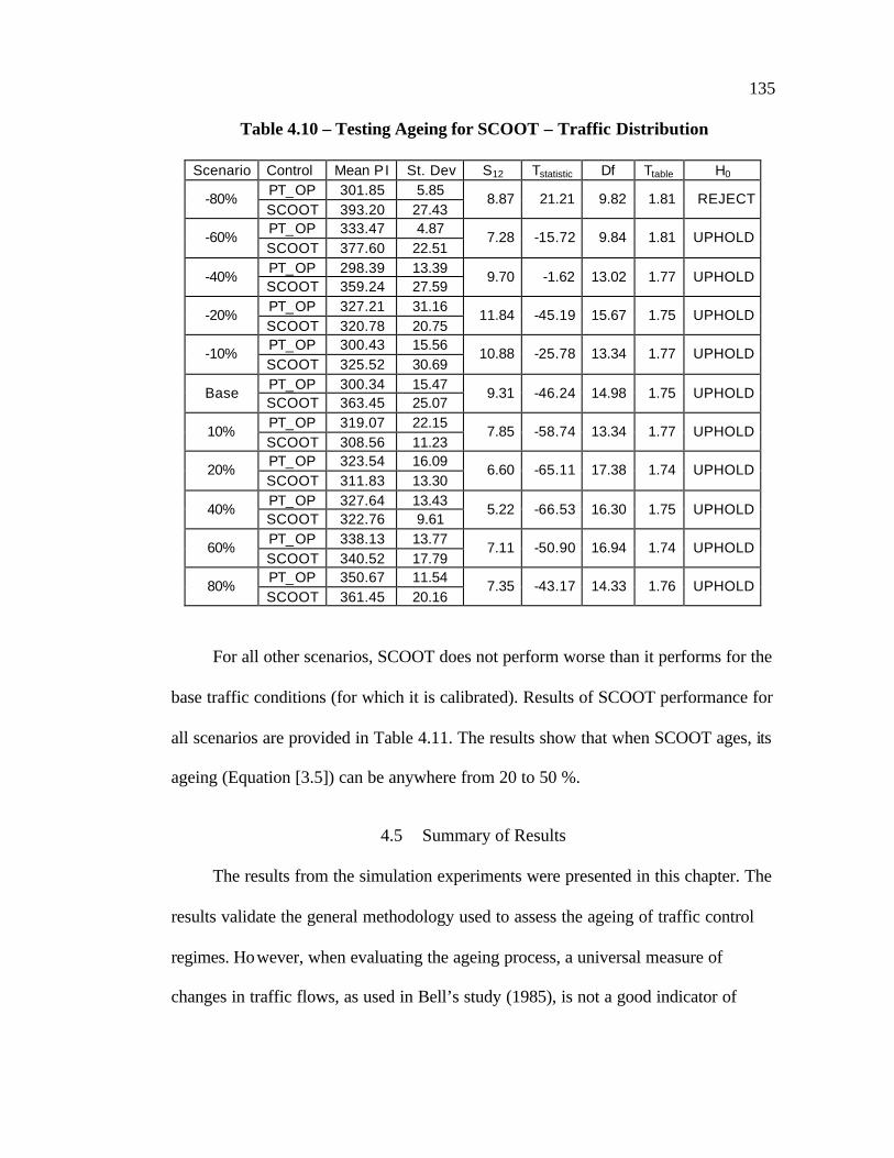
135
Table 4.10 – Testing Ageing for SCOOT – Traffic Distribution
Scenario Control Mean PI St. Dev S12 Tstatistic Df Ttable H0 PT_OP 301.85 5.85
-80% SCOOT 393.20 27.43
8.87 21.21 9.82 1.81 REJECT
PT_OP 333.47 4.87 -60%
SCOOT 377.60 22.51 7.28 -15.72 9.84 1.81 UPHOLD
PT_OP 298.39 13.39 -40%
SCOOT 359.24 27.59 9.70 -1.62 13.02 1.77 UPHOLD
PT_OP 327.21 31.16 -20%
SCOOT 320.78 20.75 11.84 -45.19 15.67 1.75 UPHOLD
PT_OP 300.43 15.56 -10%
SCOOT 325.52 30.69 10.88 -25.78 13.34 1.77 UPHOLD
PT_OP 300.34 15.47 Base
SCOOT 363.45 25.07 9.31 -46.24 14.98 1.75 UPHOLD
PT_OP 319.07 22.15 10%
SCOOT 308.56 11.23 7.85 -58.74 13.34 1.77 UPHOLD
PT_OP 323.54 16.09 20%
SCOOT 311.83 13.30 6.60 -65.11 17.38 1.74 UPHOLD
PT_OP 327.64 13.43 40%
SCOOT 322.76 9.61 5.22 -66.53 16.30 1.75 UPHOLD
PT_OP 338.13 13.77 60%
SCOOT 340.52 17.79 7.11 -50.90 16.94 1.74 UPHOLD
PT_OP 350.67 11.54 80%
SCOOT 361.45 20.16 7.35 -43.17 14.33 1.76 UPHOLD
For all other scenarios, SCOOT does not perform worse than it performs for the
base traffic conditions (for which it is calibrated). Results of SCOOT performance for
all scenarios are provided in Table 4.11. The results show that when SCOOT ages, its
ageing (Equation [3.5]) can be anywhere from 20 to 50 %.
4.5 Summary of Results
The results from the simulation experiments were presented in this chapter. The
results validate the general methodology used to assess the ageing of traffic control
regimes. However, when evaluating the ageing process, a universal measure of
changes in traffic flows, as used in Bell’s study (1985), is not a good indicator of

136
Table 4.11 – Overall SCOOT Performance
Scenario Control Mean PI Difference SCOOT vs. PT_OP Ageing γ
(% Ageing) PT_OP 300.34 Base SCOOT 363.45
63.11 NA NA NA
PT_OP 168 -25% TD SCOOT 209.86
41.86 Worse No Ageing NA
PT_OP 165.38 -20% TD SCOOT 229.55
64.17 Worse No Ageing NA
PT_OP 200.38 -15% TD SCOOT 241.82
41.44 Worse No Ageing NA
PT_OP 231.42 -10% TD SCOOT 262.18
30.76 Worse No Ageing NA
PT_OP 258.25 -5% TD SCOOT 283.16
24.91 Worse No Ageing NA
PT_OP 371.98 5% TD SCOOT 361.95
-10.03 Better No Ageing NA
PT_OP 446.13 10% TD SCOOT 523.19
77.06 Worse Ageing 18.1
PT_OP 564.04 15% TD SCOOT 629.49
65.45 Worse No Ageing NA
PT_OP 626.16 20% TD SCOOT 748.35
122.19 Worse Ageing 48.35
PT_OP 744.18 25% TD SCOOT 840.88
96.7 Worse Ageing 34.73
PT_OP 301.85 -80% TM SCOOT 393.2
91.35 Worse Ageing 30.91
PT_OP 333.47 -60% TM SCOOT 377.6
44.13 Worse No Ageing NA
PT_OP 298.39 -40% TM SCOOT 359.24
60.85 Worse No Ageing NA
PT_OP 327.21 -20% TM SCOOT 320.78
-6.43 Better No Ageing NA
PT_OP 300.43 -10% TM SCOOT 325.52
25.09 Worse No Ageing NA
PT_OP 319.07 10% TM SCOOT 308.56
-10.51 Better No Ageing NA
PT_OP 323.54 20% TM SCOOT 311.83
-11.71 Better No Ageing NA
PT_OP 327.64 40% TM SCOOT 322.76
-4.88 Better No Ageing NA
PT_OP 338.13 60% TM SCOOT 340.52
2.39 Worse No Ageing NA
PT_OP 350.67 80% TM SCOOT 361.45
10.78 Worse No Ageing NA

137
changes in traffic flows.
Evaluation of ageing for pretimed and actuated traffic control regimes show
that both of these regimes deteriorate with changes in traffic flows. The benefits of
retiming signal timing plans, which come as a consequence of the deterioration
process, show that updating pretimed traffic control is more beneficial than updating
actuated traffic control. Assessment of SCOOT ageing shows that performance of this
control regime highly fluctuates with changes in traffic flows. The ageing process is
recognized and quantified based on performance for the initial condition. The
SCOOT control performs worse than optimized pretimed control for most of the
scenarios but it ages only for few extreme scenarios.

CHAPTER 5
DISCUSSION
This chapter discusses the results presented in the previous chapter. First, the
general methodology used to assess the ageing of traffic control is discussed. Next,
the ageing measure used by Bell is discussed, along with the reason for its failure to
provide a reliable measure of aged traffic flows. The third part of this chapter
discusses the results of assessed ageing of pretimed and actuated traffic control
regimes. Specific reasons for the particular results are provided. The last part of the
chapter discusses the ageing of the SCOOT control regimes.
5.1 Methodology for Assessing the Ageing of Traffic Control Regimes
The methodology developed to assess the ageing of different traffic control
regimes for various changes in traffic flows works well for most cases. Figure 4.1
proves the idealized concept of ageing which was introduced at the beginning of the
Methodology chapter (Figure 3.1). However, selection of appropriate tools for
assessing ageing reveals some deficiencies in the concept. In order to have a clear
distinction between performance of optimized and nonoptimized timing plans, one
should use a microsimulation software that endorses use of these plans. This is often
not the case. Only a few microsimulators endorse optimized timing plans from
macroscopic optimization tools like Synchro and TRANSYT-7F.
139
Although adjustment of microsimulators to endorse the use of macroscopically
optimized timing plans seems like the only feasible approach, this is not the case.
Adjustment of the microsimulation is a tedious and complex process which, in the
end, might not give good results. There are two reasons for this. First, traffic models
embedded into microsimulations are much more complex and are founded on
stochasticity of traffic flows. Therefore, it is a question of whether they can be
properly adjusted at all. Second, the MOEs used to express the performance of macro
and micro simulators are often not in accordance. If the macroscopically optimized
timing plans were going to be endorsed by microsimulation tools, the MOEs should
be adjusted as well.
The particular difficulties of this study are associated with an inability to
validate use of Synchro’s actuated-coordinated timing plans in VISSIM. Once
validated to endorse pretimed plans for assessing the ageing of the SCOOT control,
VISSIM could not be adjusted to endorse actuated-coordinated timing plans. Future
research should go in the direction of developing VISSIM microscopic optimization
(similar to Direct CORSIM optimization). If the microscopic VISSIM optimization
had been available, it would be possible to compare pretimed, actuated, and SCOOT
control with more accuracy.
Another deficiency in the methodology is associated with the SCOOT ageing
concept. The ageing of SCOOT is based on the difference between SCOOT control
and pretimed control for a base traffic condition. In this particular study, the
difference for the base condition was quite high. The ageing of SCOOT was defined
as a situation where the difference (between SCOOT and pretimed control) for some

140
new traffic conditions exceeds the base difference. This did not occur many times for
the given traffic conditions, making SCOOT look good. If this difference had been
smaller for the base traffic conditions (which might happen for other network and
traffic configurations), then SCOOT would age more.
5.2 Reliability of the Ageing Measure for Changed Traffic Flows
The concept of the CF ageing measure is proven to be an unreliable indicator of
the possible benefits of updating signal timings. The CF concept used in Bell’s study
(1985) and in this research is based on the absolute differences in link flows for
existing and aged traffic flows.
When used to identify the relationship between deterministic changes in traffic
flows and the benefits of updating timing plans, the CF correlates well with the
benefits of retiming (Figures 4.2 to 4.5). However, deterministic changes in traffic
flows are very rare on real road networks. When several simultaneous random
variations are introduced in traffic flows, the CF fails to correlate the benefits of
retiming signal plans. One can clearly see from Figure 4.6 that various CF measures
are scattered all over the graph, covering various ranges of signal retiming benefits.
Figures 4.2 to 4.5 show that the same CF values for various deterministic experiments
yielded different benefits of signal retiming. This finding shows that the CF, as a
unique measure of changes in traffic flows, cannot be used to correlate these changes
with the benefits of signal retiming as in Bell’s study (1985).
The major reason for the CF’s inability to reflect ageing of traffic signal timing
plans lies in its definition. By definition, CF equally accounts for changes in left,

141
through and right movements. In reality, however, an additional vehicle in the left
turn lane could cause much more congestion than the through or right moving
vehicle. Therefore, the benefits of updating signals for the additional left turn vehicle
could be much higher than for the other two cases.
5.3 Ageing of Pretimed and Actuated Traffic Control Regimes
The next subsections discuss the results of the ageing of pretimed and actuated
traffic controls presented in section 4.3 of the previous chapter.
5.3.1 Deterministic Traffic Demand and Distribution Scenarios
5.3.1.1 Decrease in Traffic Demand
5.3.1.1.1 Pretimed Traffic Control. The results for the impact of a decrease
in traffic demand on the pretimed traffic control regime are shown in Figures 4.7, and
4.11 and Table 4.1. These results were also previously shown in Figure 4.2. The
results show that optimized timing plans yield a smaller PI than nonoptimized timing
plans. The exceptions to this are reductions in traffic demand by 5% and 25%. For a
5% reduction in traffic demand, nonoptimized timing plans are probably good enough
so that no benefits are achieved by optimization. For a decrease of 25%, different
underlying reasons cause no benefits of updating signal timings. The outliers shown
in Figure 4.2 coincide with no benefits of updating pretimed control regimes for a
25% decrease in traffic demand. These outliers represent a case where traffic demand
decreases further, but there are no benefits of retiming pretimed signals. This is
because of the limitations of the optimization set by the lowest possible cycle length.

142
In other words, the benefits of optimizing will be zero if the demand falls so low that
it requires an optimal cycle length that is lower than the minimum cycle length.
5.3.1.1.2 Actuated-Coordinated Traffic Control. The results for the impact of
a decrease in traffic demand on the actuated traffic control regime are shown in
Figures 4.9 and 4.11 and Table 4.3. For this traffic control regime, there are benefits
of updating signal timings for any scenario except for a 5% decrease in traffic
demand. Unlike pretimed traffic control, this control regime still yields benefit from
retiming their settings for a 25% decrease in traffic demand. This comes from the fact
that during some cycles, green splits will be utilized better with a lower traffic
demand. Pretimed traffic control has no such flexibility, so it cannot adjust further
unless the cycle length is reduced.
5.3.1.2 Increase in Traffic Demand
5.3.1.2.1 Pretimed Traffic Control. The impacts of an increase in traffic
demand on the pretimed traffic control regime are shown in Figures 4.7, and 4.12 and
Table 4.1. The results show that optimized timing plans yield a smaller PI than the
nonoptimized timing plans for all scenarios but the one where the traffic demand
increases by 5%. This result for the 5% scenario is again a consequence of the fact
that the changes in traffic flows are so small that no benefits are achieved by
optimization. Table 4.1 and Figure 4.12 support such findings. Figure 4.12 also
shows that the benefits of updating signal timings do not grow after a certain point (in
this case, after a 25% increase in traffic demand). This finding is simply a
consequence of the fact that once the saturation point in the network is reached, the

143
benefits of retiming signals will no longer increase. Still, major attention should be
given to the part of the graph where the relationship between the benefits and demand
is linear. This addresses ageing pretty well for most traffic systems because the traffic
demand does not increase more than 20% over 3 to 5 years.
5.3.1.2.2 Actuated-Coordinated Traffic Control. The impacts of an increase
in traffic demand on the actuated traffic control regime are shown in Figures 4.9, and
4.12 and Table 4.3. The results are very similar to those of pretimed traffic control.
Both pretimed and actuated traffic control regimes are incapable of coping with
increased traffic demand without increasing cycle lengths.
5.3.1.3 Decrease in Turning Movements
5.3.1.3.1 Pretimed Traffic Control. Figures 4.8 and 4.13 and Table 4.2 show
the impacts of a decrease in turning movement proportions on the performance of the
pretimed traffic control regime. The benefits of retiming traffic signals for these
changes come from reallocation of the green splits. More green time is needed for
through movements to compensate for the increase in traffic resulting from the
decrease in left and right turning movements. Table 4.2 shows that all decreases in
turning movement proportions endorse updates of signal timings. According to Table
4.2, updating signal timings for all scenarios of decrease in turning movements yield
significant benefits.
5.3.1.3.2 Actuated-Coordinated Traffic Control. Figures 4.10 and 4.13 and
Table 4.4 show the impacts of a decrease in turning movement proportions on the
performance of the actuated traffic control regime. Figure 4.10 shows no difference

144
between optimized and nonoptimized actuated signal timings when turning
movement proportions are decreased. Table 4.4 formally shows that the differences
are not significant. Similarly, Figure 4.13 shows no benefits of optimization of signal
timing plans for these scenarios. One could conclude that the traffic control does not
perform well for these changes in traffic flows. However, the opposite is true. For the
pretimed control (Figures 4.8 and Table 4.2), the benefits of retiming traffic signals
come from reallocation of green splits and the increase in cycle length for the heavy
through movements (80% decrease in turning movements). However, actuated-
coordinated traffic control does not need retiming of splits and cycle length. The
benefits of retiming actuated control are negligible because, with very low traffic
demand for left turns during certain cycles, left phases are skipped and all green time
is used for heavy through movements. For pretimed control, left phases cannot be
skipped and an increase in cycle lengths is required to accommodate those through
movements.
5.3.1.4 Increase in Turning Movements
5.3.1.4.1 Pretimed Traffic Control. Figures 4.8 and 4.14 and Table 4.2 show
the impacts of an increase in turning movement proportions on the performance of
the pretimed traffic control regime. The benefits of retiming traffic signals for these
changes also come from reallocation of the green splits. More green time is needed
for left turns (right turns on red are allowed) to compensate for an increase in traffic
for the left turn movements. Table 4.2 shows that a small increase of 10% in turning
145
movement proportions produces no benefits of updating signal timings. Updating
signal timings for other scenarios yield significant benefits.
5.3.1.4.2 Actuated-Coordinated Traffic Control. Figures 4.10 and 4.14 and
Table 4.4 show the impacts of an increase in turning movement proportions on the
performance of the actuated traffic control regime. Table 4.4 shows that all increases
in turning movement proportions endorse updates of signal timings. Figure 4.14
shows that the benefits of updating are smaller for actuated-coordinated control than
for pretimed traffic control. The reason for this difference is that the actuated-
coordinated control performs better for higher increases in turning proportions.
Actuated traffic control will use all gaps in through traffic to pass more left-turning
vehicles more, if possible. The pretimed control has no such flexibility. Therefore,
once the signal timings are updated, the benefits of updating are higher for pretimed
control. In general, whenever flexibility of actuated traffic control can be used to
cope with changes in traffic conditions, the benefits of updating settings for this
control are lower than for pretimed control.
5.3.1.5 Discussion on Other Findings for Deterministic Scenarios
Two other major findings can be taken from the results presented in Figures
4.2 – 4.14. First, the benefits of updating are higher for optimization of traffic flows
with increased demand than for optimizing the traffic flows with decreased demand.
This means that it is better to optimize signal timings for a traffic demand that is
higher than the current traffic demand. The disbenefits of such an optimization are

146
smaller than the disbenefits of having outdated signal timing plans when the traffic
demand increases. This finding confirms the findings of Park et al. (2000).
Second, it seems that the benefits of updating timing plans when only turning
movements have been changed (split optimization) are higher than the benefits of
updating timing plans when only traffic demand has been changed (cycle length
optimization). This finding emphasizes the importance of actuated traffic control.
Actuated traffic signals account fo r the majority of changes in turning movement
proportions by adjusting phase splits according to turning movement demand during
each cycle. According to the results of this study, if updating of splits is unnecessary
and traffic demand at the links is uniformly increased, the benefits of updating signal
timings are limited to no more than 2-3% per year for up to a 5% increase in overall
traffic demand.
5.3.2 Stochastic Traffic Demand and Distribution Scenarios
The results for stochastic changes in traffic demand and turning movements
presented in Figure 4.15 are quite different from those for uniform deterministic
changes. For example, for a 0 to 5% increase in traffic demand, the minimum benefits
of updating the timing plans are around 15% for pretimed control, or 5% for actuated-
coordinated control. These benefits are much higher than the benefits for a
deterministic increase in traffic demand (Figures 4.7 and 4.9). This difference is
associated with the different natures of deterministic and stochastic experiments.
While all traffic demand inputs are equal and turning proportions do not change in the
deterministic approach, all of these factors are changed randomly in the stochastic

147
approach. So, while the stochastic experiments require optimization of all signal
timing parameters (splits, offsets, and cycle length), the deterministic experiments,
whose results are presented in Figure 4.7 and 4.9, require mostly optimization of
cycle length. Therefore, the benefits of updating signal timings for stochastic
experiments are consequently higher.
Surprisingly, the results from 14 examples of successful retiming projects
(ITE 2005) show approximately 30-40% of average benefits in delay and stops when
timing plans are updated. Although this is merely a coincidence, these results prove
that the estimations of the benefits from this study are within the range of what others
found in the field.
5.4 Ageing of the SCOOT Control Regime
5.4.1 General Discussion of SCOOT Performance
In general, SCOOT performs worse than optimized pretimed plans for almost
all scenarios of changed traffic demand and distribution. Moreover, SCOOT often
performs worse than nonoptimized pretimed plans.
Before discussing possible reasons for SCOOT performing worse than pretimed
plans, here are some of the assumptions that might affect SCOOT’s performance:
• The peak-hour traffic demands used in this research were all constant during
the peak hour. SCOOT is known as a signal optimization strategy that delays
the onset of congestion and recovery from congestion. Most of SCOOT’s
SCOOT benefits likely come from these two (prepeak and postpeak) periods.
However, since traffic demand was kept constant, there were no opportunities

148
for SCOOT to benefit from these two common peak periods. Alternatively,
well prepared pretimed plans are an ideal traffic control for constant and
heavy traffic demand.
• SCOOT version 4.2 is used in this study. Version 4.5 and especially version
MC3 are likely to enable better SCOOT performance than the old version.
Newnew features (added to with version 4.5 and version MC3) that can make
a strong impact on SCOOT performance are complex links (with
supplementary detectors) and the ability to estimate saturation occupancy
online (SOFT). Had these features been used in this study, SCOOT might
have performed better.
• The SCOOT network has been validated and calibrated to the best of the
author’s knowledge. However, SCOOT is a complex system. Many years of
expertise are needed before one can get the most out of SCOOT. The purpose
of this study was not to adjust SCOOT in such a way to get the best results.
That was beyond the scope. The purpose was to build and validate SCOOT
configurations and evaluate their performance under various traffic changes
without adjusting SCOOT at all. Therefore, due to the experimental design of
this study, the results and findings of SCOOT performance should not be used
to qualify the general performance of SCOOT or compare SCOOT
performance with any traffic condition or and network different from those
used in this study.
There are several other possible reasons for the fact that SCOOT performs
worse than nonoptimized pretimed plans:

149
• SCOOT control settings perform worse than nonoptimized timing plans
• The PIs of pretimed control in VISSIM could be overestimated. Therefore,
SCOOT could have been better than nonoptimized timing plans if VISSIM
had been adjusted to endorse timing plans from Synchro in the same way that
SimTraffic is adjusted
However, one should not focus on the fact that SCOOT is sometimes worse
than nonoptimized performance of pretimed control. Comparison of SCOOT
performance and performance of optimized pretimed plans is essential for
determining the ageing of the SCOOT control. However, before discussing the ageing
of SCOOT, it is necessary to discuss the fact that SCOOT performs worse than
optimized pretimed control (Figure 4.16 and Figure 4.7).
There are two major reasons that cause SCOOT to perform worse than
optimized pretimed control. Each of these reasons can be divided further. The reasons
are:
• SCOOT signal optimization strategies are not the best for current traffic
conditions
• SCOOT does not model traffic properly and, therefore, signal timing
adjustments are inadequate
The next subsections describe the failures of SCOOT optimization strategies
and SCOOT’s inability to model traffic properly.

150
5.4.1.1 Failures of SCOOT Optimization Strategies
There are two reasons why the SCOOT optimization strategies might not be the
best for traffic changes modeled in this study. The first reason is associated with
small unnecessary fluctuations of SCOOT signal timings. The second reason is
related to selection of the best cycle lengths, which provide good traffic progression
in the network.
5.4.1.1.1 Fluctuations of SCOOT Signal Timings. SCOOT is an adaptive
traffic control system that adjusts to changes in traffic demand and distribution in real
time. Over years, a time span characteristic for any ageing process, this system should
not have problems in adjusting to traffic changes. In fact, SCOOT usually needs just
15 – 20 minutes (the time which was used for VISSIM simulation warm-ups) to
adjust from initial timing settings to the timing settings “appropriate” for surrounding
traffic conditions. The approach that SCOOT uses to determine the “appropriate”
timing settings is another issue.
The simulation experiments have shown that SCOOT has no problem in
adjusting to existing traffic conditions in the way the SCOOT model finds it is the
best. However, SCOOT control will not remain constant after timings are adjusted to
surrounding traffic conditions. The SCOOT control will continue to fluctuate by
changing cycle lengths, offsets and splits to respond to short time variations in traffic.
These fluctuations of SCOOT signal timings are counter effective over a longer time
period (1 or 2 hours) with constant traffic demand. They yield more costs than
benefits. All experiments conducted in this research assume constant traffic demand
over a 1-hour peak period (different levels, but always constant along the time

151
period). However, even the constant traffic demand is modeled with some variations
in micro simulators. These variations will cause 5-minute hourly traffic rates to not be
constant during the whole hour. These various 5-minute hourly traffic rates are large
enough to trigger a fluctuation in SCOOT control. SCOOT changes its cycle lengths
every 2.5 to 5 minutes. Other timing settings are changed even more frequently. In
this way, SCOOT timings oscillate around their mean values, which are close to the
ones defined by pretimed optimized traffic control.
These fluctuations in SCOOT’s signal timings, although small, affect the
smoothness of existing traffic progression by causing additional delays and stops. The
consequences of such changes are termed “transients”. When changes in SCOOT’s
signal timing settings are triggered by small and negligible changes in traffic flows,
the transients mean more delays and stops than benefits. The increase in stops and
delays during each cycle might be negligible, but their accumulation at the end of the
simulation period is large enough to overcome delays and stops produced by
optimized pretimed plans.
5.4.1.1.2 Selection of Cycle Lengths. Shelby et al. (2005) investigated the
impact of selection of cycle lengths on traffic performance on arterial streets. The
authors compared “system friendly” cycle lengths with strictly flow proportionate
approaches in selecting cycle length referred to as the “90% rule”. The “90% rule”
represents a way of selecting cycle lengths used by most of the existing adaptive
control systems in the USA. Systems like SCOOT (Hunt et al., 1981), SCATS
(Lowrie, 1982) and OPAC (Gartner, 1983) all use the “90% rule” when selecting
cycle lengths for multi- intersection network configurations. The rule means that a

152
critical intersection will govern the cycle length of the whole network by keeping the
degree of saturation at 90%. If an intersection becomes more than 90% saturated (and
reallocation of splits cannot reduce this value), then the common cycle length for the
whole network is increased by a few seconds. Similarly, the cycle length decreases if
saturation falls below 90%. Although this follows the trends in traffic demand, it does
not always yield the best cycle lengths. For certain network configurations, only a
few cycle lengths provide good progression for both directions of major network
arterials. If the selected cycle length is different from the cycle lengths which give the
best progression, the traffic performance is suboptimal.
Shelby et al. (2005) used the notion of a “resonant cycle” for those cycle
lengths that accommodate good two-way arterial progression. They found that the
“resonant cycles” yield benefits of up to 40% fewer delays when compared with the
cycles selected by the “90% rule”. The authors also found that, even if resonant
cycles are not present (no cycles which provide good two-way progression), well-
chosen cycle lengths may still outperform the cycles chosen by using the “90% rule”.
These findings seriously question SCOOT’s strategy for optimizing network cycle
length.
It has been noted in this study that the SCOOT cycle lengths are greater, on
average, than the cycle length used in optimized pretimed plans. Larger cycle lengths
increase the capacity of the network (only up to a certain point), but they also
increase delay for all vehicles in the network. The almost constant difference between
SCOOT’s performance and the performance of optimized pretimed control, shown in

153
Figure 4.16, shows that SCOOT’s inadequate selection of cycle lengths could be one
of the reasons for this discrepancy.
5.4.1.2 Failures of SCOOT Traffic Modeling
The section “SCOOT Validation” describes the fundamentals of SCOOT traffic
modeling and the necessary adjustments that need to be made for SCOOT to
accurately estimate vehicles at intersection approaches. It has been noted during the
simulations that SCOOT keeps some green times longer or shorter than necessary.
Green times for each phase depend on cycle length, but they are mostly adjusted
based on cyclical demand for each phase.
Initial validation efforts have shown that SCOOT has been properly validated
(Figure 3.25). Several experiments were done to check SCOOT’s accuracy in
estimating approaching vehicles at the intersections for changed traffic conditions.
SCOOT estimates approaching vehicle s based on average travel time (from detector
to stop line), the assumed platoon progression factor, etc. All these factors are
dependant on the intensity of traffic flows, which can be represented by the scenarios
of changes in traffic demand used in this study. Scenarios representing changes in
traffic distribution are not essential for checking SCOOT’s ability to accurately
estimate approaching vehicles. Therefore, 11 scenarios of changes in traffic demand
are used to model traffic. Queue measures for both SCOOT (modeled) and VISSIM
(“real”) are taken. For each of nine intersections, SCOOT and VISSIM queues are
measured during 10 minutes for each of 11 scenarios. The same 10-minute intervals

154
are used to measure queues for each intersection, keeping the measurements
consistent.
Similar results to those presented in Figure 3.25 are obtained for all 11 traffic
demand levels. After the data reduction, a set of the least square models are
developed for the 11 scenarios to represent correlation between modeled and actual
number of vehicles in queues (see APPENDIX). Figure 5.1 shows the results from
these experiments. The base traffic demand is represented by the zero point on the X
axis. The least square model for this traffic demand is developed from experiments
done for initial validation of the SCOOT model. Figure 5.1 shows the number of
vehicles estimated by the SCOOT model for 100 actual vehicles (VISSIM). SCOOT
50
60
70
80
90
100
110
120
130
140
150
-25 -20 -15 -10 -5 0 5 10 15 20 25Change in Traffic Demand (%)
Num
ber
of V
ehic
les
from
SC
OO
T M
odel
0
0.1
0.2
0.3
0.4
0.5
0.6
0.7
0.8
0.9
1
Coe
ffici
ent o
f Det
erm
inat
ion
SCOOT Vehicles
Actual Vehicles
Coefficient of Determination
Figure 5.1 – Accuracy of SCOOT Traffic Model vs Traffic Demand

155
estimation for base traffic conditions is close to the actual number of vehicles.
SCOOT estimates around 97 vehicles for every 100 actual vehicles. However, as
traffic demand changes, the least square models become less accurate. When traffic
demand increases, SCOOT tends to overestimate the number of vehicles. For
example, for a 15% increase in traffic demand, SCOOT will estimate 145 vehicles for
every 100 actual vehicles. For scenarios of decreased traffic demands, the error will
be smaller. However, Figure 5.1 clearly shows that SCOOT’s ability to model the
approaching vehicles at the intersections degrades with changes in traffic demand. All
of the least square models that have been developed from the queue observations are
quite reliable, having coefficients of determination between 0.73 and 0.85.
The findings from these experiments show that SCOOT’s traffic model mostly
overestimates the number of approaching vehicles. The consequences of this
overestimation are improper green splits and a tendency to increase cycle length in
the region. When SCOOT overestimates the number of vehicles approaching the
intersection during one phase, this information is conveyed to the SCOOT optimizers,
which will consequently impose an unnecessary, longer green time for the phase. If a
similar situation occurs for each phase, the cycle length will be increased. So,
accuracy of the SCOOT model highly impacts the efficiency of the SCOOT traffic
signal control. With that in mind, the results presented in Figure 5.1 prove the
existence of SCOOT ageing, which has its roots not in traffic control, but in SCOOT
modeling of traffic flows.

156
5.4.2 SCOOT Ageing for Changes in Traffic Demand
Figure 4.16 and Tables 4.6 and 4.7 show the impacts of changes in traffic
demand on the performance of SCOOT and pretimed traffic control regimes. Table
4.6 shows that SCOOT is coincidentally better than optimized pretimed control only
for the scenario of a 5% increase in traffic demand. For all other scenarios, SCOOT is
significantly worse than the pretimed traffic control.
Table 4.7 shows that SCOOT does not age for most of the scenarios.
However, these findings are more an indication of the difference between SCOOT
and pretimed performance for base traffic conditions than a proof that SCOOT does
not age. In fact, the difference between PIs for SCOOT and pretimed control is pretty
high for base traffic conditions. Since the difference is so high, it is only exceeded a
few times for increases in traffic demand of 10, 20, and 25% (for 15%, the amount
that the difference is exceeded is not significant). However, when the difference is
exceeded, it contributes to high coefficients of SCOOT ageing of 18, 48, and 35% for
respective increases in traffic demand (Table 4.11).
5.4.3 SCOOT Ageing for Changes in Traffic Distribution
Figure 4.17 and Tables 4.9 and 4.10 show the impacts of changes in traffic
distribution on the performance of SCOOT and pretimed traffic control regimes.
Table 4.9 shows that for several changes in turning movement percentages (-20, 10,
20, and 40%), the SCOOT control is better than optimized pretimed control. This is
not a coincidence. SCOOT shows quite consistent performance for most of the traffic

157
distribution scenarios. This consistency and the fact that for these scenarios SCOOT
control is often better than pretimed control are the consequences of two factors.
First, when total traffic demand in the network is kept constant, all increases
in turning movements cause decreases in through movements. When through traffic is
decreased, this is equivalent to a decrease in traffic demand for only the through
movements. Figure 5.1 already showed that SCOOT accuracy is better for reduced
traffic demand than for increased traffic demand. Therefore, SCOOT performs better
for increased turning movements. Prove of this statement is visib le in the left part of
Figure 4.17. For high decreases in turning movements, the through traffic is increased
so much that SCOOT again starts producing unreliable estimates of the traffic and
consequently leads to poorer performance (Figure 4.17 – Scenarios -40, -60, -80%).
The second reason for improved SCOOT performance is that SCOOT behaves
in a certain way as an actuated traffic control. The phases cannot be skipped
(although the real SCOOT can make some phases demand-dependent), but left turn
greens can be extended to satisfy varying traffic demand. This fact represents a
benefit over pretimed control, which cannot vary green times for various left turn
demand levels.
Unlike for changes in traffic demand, SCOOT is always better than
nonoptimized pretimed timing plans for any change in turning movement
proportions. This proves that the SCOOT control regime can respond very
successfully to long term changes in turning movements.
Figure 4.8 shows that SCOOT does not age for most of the changes in turning
movement proportions. The fact that SCOOT ages for a 80% decrease in turning

158
movements is not surprising. A reduction of 80% in left and right turns for the base
network traffic demand is equivalent to an increase of 22% for through traffic
demand at each intersection approach. Figure 4.16 and Table 4.7 show that for such
high increases in traffic demand, SCOOT does age. The ageing coefficient for this
scenario is around 30%, which is comparable to previous results (Table 4.11).
One important issue has to be mentioned when discussing SCOOT ageing for
changes in turning movements. Idealized detector placements are used to configure
left turns in the SCOOT system. Usually, SCOOT uses filter links to determine green
times necessary for left turns. This concept retrieves information on the number of
left turning vehicles during the previous cycle when determining the duration of the
left turn green time for the current cycle. Detectors are placed on the filter links,
which are usually downstream links that the left-turn vehicles turn onto (Siemens
2003). When this concept is used, SCOOT does not provide proactive green time for
left turn movements, but the green time is based on the demand from the previous
cycle.
The SCOOT system configured in this study treats left turn movements as all
other (through) movements. This means that the detectors are placed in the left turn
pockets, well ahead of the stop line. This concept enhances split optimization of the
left turns. However, placement of the detectors is more important from another
aspect. SCOOT detectors, which are placed close to the upstream intersections,
usually detect all vehicles approaching the intersection. When these vehicles come
closer to the intersection, they split entering turning movement pockets (left and
right). Therefore, the actual number of through vehicles that arrive at the intersection

159
could be considerably lower than the number of detected vehicles. This inconsistency
negatively impacts the accuracy of the SCOOT traffic model. The new SCOOT
version MC3 allows installation of additional detectors to deduct turning vehicles.
For older SCOOT versions (SCOOT 4.2 is used for this study), this problem is
supposed to be solved by adjusting the saturation occupancy parameter STOC. STOC
is supposed to be increased enough so that it accounts for vehicles that turn left and
right at the intersection. However, a regular STOC validation is complex enough that
this additional adjustment brings a higher potential for error. Often, validation of
STOC for such conditions is almost impossible. Even when possible, such validation
is highly dependent on the variability of turning movement proportions.
In order to avoid such problems, the SCOOT detectors in this study are placed
unconventionally. Both left turn and through detectors are placed at the entrances to
the left and right turning pockets (Figure 3.24). This distance is approximately 450 ft
from the stop bars. The through detectors are placed after the entering points into left-
turn pockets. In this way, only through vehicles are detected by “through” detectors
and validation of STOC can be completed with higher accuracy. Description of this
concept is important because, if the detectors had not been placed this way, SCOOT
would not show such good results when assessing SCOOT ageing for the traffic
distribution scenarios.
5.5 Summary of Discussion
Discussion of the results was presented in this chapter. The general
methodology used to measure the ageing of various traffic control regimes is viable.

160
However, there are a few deficiencies. First, the results of the ageing process are
quite dependent on adjustments of traffic model parameters and MOEs from macro
and microsimulation tools. Second, the ageing of SCOOT is assessed in a way that
largely depends on the difference between SCOOT and pretimed performance for the
base traffic conditions. This approach shows that SCOOT performs better than it
really does.
Further, the ageing measure introduced by Bell (1985) is discussed. This
measure does not uniquely correlate changes in traffic flows with changes in
performance of a traffic control regime. Therefore, the experimental results reported
in Bell’s study should be taken with reserve.
The ageing of pretimed and actuated controls is discussed in the next section of
the chapter. In general, actuated-coordinated control always performs better than
pretimed control. Therefore, the benefits of retiming actuated-coordinated control are
always smaller than for pretimed control.
SCOOT performance is discussed in the last part of the chapter. Several reasons
are discussed for SCOOT performance being worse than the pretimed performance.
The reasons are associated with deficiencies in both SCOOT optimization strategies
and the way SCOOT models traffic at the intersection approaches. The results show
that accuracy of the SCOOT traffic model degrades with changes in traffic demand.
Bell’s ageing results (Bell, 1985) from real networks (around 3% per year,
with up to four years between updates) are frequently used when the disbenefits of
not optimizing signal timings need to be estimated. The results from this research

161
show that Bell’s estimate should not be used for any situation. There are two reasons
why the estimate of 3% should not be used anywhere.
First, the disbenefits of deterioration of traffic signal timings should not be
associated with the time elapsed from the last retiming process. Time itself is not a
factor that influences deterioration of traffic control. Instead, the disbenefits of
deterioration of traffic signal timings should be associated with changes in traffic
demand and distribution. Neither Bell’s research nor this study has found a single
measure of changes in traffic flows which could successfully correlate the disbenefits
of deterioration. However, an increase or decrease in background traffic demand can
be a simple qualifier of changes in traffic flows. The results from this study show that
for every 5% increase in background traffic demand, the benefits of updating signal
timings are 3%. These results coincide with Bell’s results only if traffic demand
increases 5% per annum.
Second, the results of from this study show that the benefits of updating signal
timings can be much higher if the distribution of traffic within the network is
significantly changed. The benefits of updating signal timings when left and right
turning movements are increased can reach 50%. These distribution changes in traffic
flows are not common for most urban networks, but they are not impossible. For such
cases, Bell’s results underestimate the benefits of updating traffic signal timings.
The highly stochastic results of the research presented in the dissertation have
shown that the benefits of updating signal timings can be 35 – 45 %. Experiments that
yielded to these results were random and not common for regular road networks.
However, these results show that the ageing of timing plans can produce disbenefits

162
that are much higher than 3% per year, depending on how much traffic distribution
has changed (permanently) from the last retiming process.

CHAPTER 6
CONCLUSIONS
This chapter consists of two sections. In the first section, the conclusions of the
research are presented. The second section provides the limitations of the research, as
well as direction for future research.
6.1 Conclusions
This section presents the conclusions of an investigation on the ageing of
pretimed, actuated-coordinated, and SCOOT traffic control regimes through the use
of simulation. The research had two objectives. The first was to introduce and
validate the theoretical concept of ageing of traffic control. The second objective was
to estimate the ageing of the three traffic control regimes for a variety of deterministic
and stochastic changes in traffic demand and distribution. The following conclusions
are reached in this study.
6.1.1 Methodology for Assessing Ageing of Signal Timing Plans
The PI difference between updated (optimized) and not updated (non-
optimized) timing plans is proven to be a reliable measure of change in traffic
performance for aged traffic conditions. However, there were two problems
associated with use of the PI measure:
• It does not work very well when traffic in the network is saturated or close to
saturated. However, when traffic is saturated most traffic agencies,

164
responsible for maintenance of traffic signals, act. The real benefits of
retiming traffic signals come from conditions where ageing is unnoticed, with
small and gradual changes in traffic conditions.
• In order to have a clear distinction between PI for optimized and
nonoptimized timing plans, one should use a type of microsimulation software
that endorses use of these plans. Only the Synchro-SimTraffic combination
works fine. Other macro-micro combinations need adjustment of both traffic
model settings and MOEs.
In addition to these problems, the CF ageing measure (used by Bell) is not
proven to be a good measure of changes in traffic flows. The same CF value can yield
several different benefits of updating timing plans. This measure can be used to
assess the impact of a single deterministic change in traffic flow on traffic
performance in the network. However, the CF ageing measure fails to correlate well
with the benefits of updating timing plans if several traffic changes (stochastic
variations of demand and distribution) are combined.
6.1.2 Ageing of Pretimed and Actuated-Coordinated
Signal Timing Plans
Two different sets of experiments were conducted to estimate the benefits of
updating signal timing plans. In the first, traffic demands and distributions were
deterministically changed from the base conditions. The results show that:

165
• The impact of the turning movement changes on the ageing of the
performance of traffic signals (up to 70%) is much higher than the impact of
the traffic demand changes (up to 30%).
• Optimizing traffic signals for higher than existing traffic demand brings more
benefits than costs, if the demand is expected to grow in future years.
• In a small coordinated grid network with constant turning movement
proportions (average values), the annual benefits of retiming traffic signals are
up to 3% for traffic growth of up to 5% uniformly over the entire network.
These benefits are negligibly smaller for the actuated traffic control than for
the pretimed traffic control.
The second set of experiments introduced the stochastic nature of ageing
through the random changes of traffic demands and turning movement proportions.
The results show that:
• The average benefits of retiming signal plans are around 35% for pretimed
control and 27% for actuated control, when traffic inputs at the network and
turning proportions are randomly changed.
• The results show that these benefits do not depend on average change in
network traffic demand, due to the highly stochastic nature of the
experiments.
• The benefits of retiming estimated in this study are in accordance with
reported benefits from the field (ITE 2005).

166
6.1.3 Ageing of the SCOOT Traffic Control Regime
SCOOT ageing was evaluated only through deterministic changes in traffic
demand and distribution. Around 210 hours of SCOOT simulations were performed.
The results show that:
• SCOOT performs worse than pretimed control for most of the changes in
traffic demand. This performance has roots in deficiencies of both
optimization strategies and traffic modeling in SCOOT.
• When idealized detector placements are used, the SCOOT control performs
better or equal to pretimed control for most of the changes in traffic
distribution. Older SCOOT versions are not likely to outperform pretimed
control if detectors are placed in traditional SCOOT positions.
• The traffic model within SCOOT fails to accurately estimate approaching
vehicles for any change in traffic demand. The accuracy is weakened more by
an increase in traffic demand than by a decrease in traffic demand.
• The ageing concept for SCOOT, which is based on the difference between
SCOOT control and pretimed control for the base traffic condition, may
underestimate the ageing of SCOOT.
• SCOOT performance varies - sometimes showing that SCOOT ages, and
sometimes showing that it does not. However, in most of these cases, SCOOT
is significantly worse than optimized pretimed plans.
• When SCOOT does age, the disbenefits of ageing are moderate. For high
traffic demand growths of 20 and 25%, the results show that if the SCOOT

167
control had been replaced by optimized pretimed timing plans, delays and
stops would be reduced by 11 to 16%.
6.2 Summary of Conclusions
The foundation of this research was set with three major hypotheses stating
that each of the traffic control regimes does not age (deteriorate). The hypotheses
were based on the case that signal timing parameters are not updated regularly. Based
on the research findings, the hypotheses are:
1. H0(1) - Pretimed traffic control plans do not deteriorate with changes in
traffic demand and distribution - REJECTED
2. H0(2) - Actuated traffic control plans do not deteriorate with changes in
traffic demand and distribution - REJECTED
3. H0(3) - SCOOT adaptive traffic control does not deteriorate with changes
in traffic demand and distribution - REJECTED
6.3 Future Research
There are several directions in which the future research on ageing of traffic
control regimes should go. More investigation is needed on the real variations in
traffic demand and distribution over several years. This would help to develop more
realistic scenarios for modeling changes in traffic demand and distribution.
In addition, there is a need to investigate the possibility of developing a single
ageing measure that would depend on changes in link flows and would be able to
correlate the benefits of updating signal timing plans.

168
Major research efforts should be made in developing a stochastic optimization
tool that would use outputs from the microsimulation to optimize signal timings.
Such a tool, which uses the Genetic Algorithm (GA) approach, exists for CORSIM
microsimulation (Direct CORSIM optimization). However, preliminary results from
this study show that the GA needs more improvement before it can be used as an
everyday tool to optimize signal timings. The areas where this procedure lacks
explanation are design of the optimization process (multilevel versus all in one) and
sensitivities of both parameters and results.
A similar stochastic optimization could be developed for VISSIM. The
stochastic optimization in VISSIM would generate signal timing plans (pretimed or
actuated) which are based on VISSIM performance outputs. This process would make
performances of optimized and nonoptimized timings much more consistent.
Development of such stochastic optimization in VISSIM would enable evaluation of
all three control types (pretimed, actuated, and SCOOT) within a single
microsimulation tool. Moreover, such stochastic optimization in VISSIM could allow
use of custom-made performance indexes, which would include not only delays and
stops, but also throughputs, queue lengths, etc.
Another direction in researching the ageing of signal timing plans is associated
with prioritizing retiming of traffic signals in the network. If signal timings are
supposed to be retimed on several corridors in the network – which corridor gets
priority? The issue becomes more complex when different facilities are compared
(e.g., 6- lane arterial versus 2-lane arterial). It would be interesting to research the
trade-off between traffic demand (6 lanes have more traffic than 2) and the time that

169
has elapsed since the last retiming process (e.g., the last retiming for the 6- lane road
was 3 years ago, while the last retiming for the 2-lane road was 7 years ago).
Regarding the accuracy of the SCOOT traffic model, this research provides
results that are difficult to correlate with the underlying dynamics of traffic flows.
Such correlation was unnecessary for this research and was beyond the research
scope. More investigation is needed to thoroughly assess the accuracy of the SCOOT
traffic model. A single intersection approach should be modeled with controlled
changes in traffic speed, vehicle mix, platoon progression, link travel time, and other
factors to investigate how each of these factors affects SCOOT accuracy to predict
the number of vehicles in queue.

APPENDIX
CORRELATIONS BETWEEN SCOOT AND VISSIM QUEUES

171
Cor
rela
tion
betw
een
SCO
OT
queu
e an
d VI
SSIM
que
ue (-
25%
Tra
ffic
Dem
and)
y =
0.90
07x
+ 1.
1173
R2 =
0.7
823
05101520
05
1015
20
SCO
OT
Que
ue [v
eh]
VISSIM Queue [veh]

172
Cor
rela
tion
betw
een
SCO
OT
queu
e an
d VI
SSIM
que
ue (-
20%
Tra
ffic
Dem
and)
y =
0.87
73x
+ 0.
9528
R2 =
0.7
655
05101520
05
1015
20
SCO
OT
Que
ue [v
eh]
VISSIM Queue [veh]

173
Cor
rela
tion
betw
een
SCO
OT
queu
e an
d VI
SSIM
que
ue (-
15%
Tra
ffic
Dem
and)
y =
0.95
47x
+ 0.
6515
R2 =
0.7
452
0510152025
05
1015
2025
SCO
OT
Que
ue [v
eh]
VISSIM Queue [veh]

174
Cor
rela
tion
betw
een
SCO
OT
queu
e an
d VI
SSIM
que
ue (-
10%
Tra
ffic
Dem
and)
y =
0.88
34x
+ 0.
9846
R2 =
0.7
483
0510152025
05
1015
2025
SCO
OT
Que
ue [v
eh]
VISSIM Queue [veh]

175
Cor
rela
tion
betw
een
SCO
OT
queu
e an
d VI
SSIM
que
ue (-
5% T
raffi
c D
eman
d)
y =
0.90
66x
+ 0.
2515
R2 =
0.8
307
0510152025
05
1015
2025
SCO
OT
Que
ue [v
eh]
VISSIM Queue [veh]

176
Cor
rela
tion
betw
een
SCO
OT
queu
e an
d VI
SSIM
que
ue (B
ase
Traf
fic D
eman
d)
y =
1.02
34x
+ 1.
2714
R2 =
0.8
396
051015202530
05
1015
2025
30
SCO
OT
Que
ue [v
eh]
VISSIM Queue [veh]
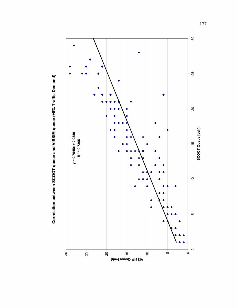
177
Cor
rela
tion
betw
een
SCO
OT
queu
e an
d VI
SSIM
que
ue (+
5% T
raffi
c D
eman
d)
y =
0.70
45x
+ 2.
0889
R2 =
0.7
365
051015202530
05
1015
2025
30
SCO
OT
Que
ue [v
eh]
VISSIM Queue [veh]

178
Cor
rela
tion
betw
een
SCO
OT
Que
ue v
s VI
SSIM
que
ue (+
10%
Tra
ffic
Dem
and)
y =
0.74
42x
+ 1.
7881
R2 =
0.8
461
0102030405060
010
2030
4050
60
SCO
OT
Que
ue [v
eh]
VISSIM Queue [veh]
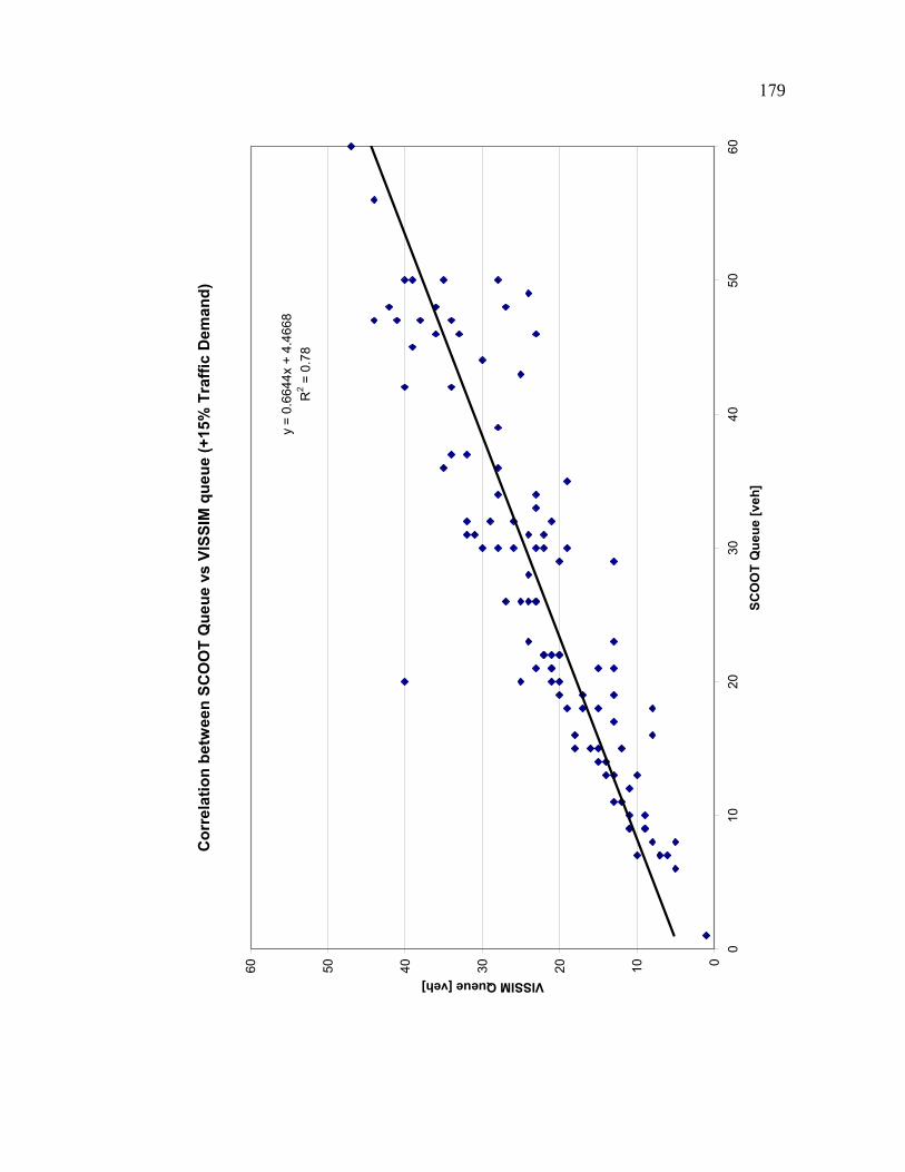
179
Cor
rela
tion
betw
een
SCO
OT
Que
ue v
s VI
SSIM
que
ue (+
15%
Tra
ffic
Dem
and)
y =
0.66
44x
+ 4.
4668
R2 =
0.7
8
0102030405060
010
2030
4050
60
SCO
OT
Que
ue [v
eh]
VISSIM Queue [veh]

180
Cor
rela
tion
betw
een
SCO
OT
Que
ue v
s VI
SSIM
que
ue (+
20%
Tra
ffic
Dem
and)
y =
0.66
16x
+ 3.
1133
R2 =
0.8
506
010203040506070
010
2030
4050
6070
SCO
OT
Que
ue [v
eh]
VISSIM Queue [veh]

181
Cor
rela
tion
betw
een
SCO
OT
Que
ue v
s VI
SSIM
que
ue (+
25%
Tra
ffic
Dem
and)
y =
0.66
16x
+ 3.
1133
R2 =
0.8
506
010203040506070
010
2030
4050
6070
SCO
OT
Que
ue [v
eh]
VISSIM Queue [veh]

182
Cor
rela
tion
betw
een
SCO
OT
Que
ue v
s VI
SSIM
que
ue (+
25%
Tra
ffic
Dem
and)
y =
0.67
82x
+ 3.
2897
R2 =
0.7
749
0102030405060
010
2030
4050
60
SCO
OT
Que
ue [v
eh]
VISSIM Queue [veh]

REFERENCES
1. Abdel-Rahim, A., Taylor, W.C., and Bangia, A. (1998). “The Impact of SCATS on Travel Time and Delay.” Paper prepared for the 8th ITS America Annual Meeting, Detroit Michigan. 2. Abraham, J. K. (2000). “SCATS Traffic Signal System.” http://www.ci.troy.mi.us/TrafficEngineering/sindex.htm. Accessed in June, 2003. 3. Akcelik, R., and Besley, M. (1998). SIDRA 5 - User Guide.
4. Bell, M.C. (1985). “Ageing of Fixed-Time Traffic Signal Plans.” Report to Transport and Road Research Laboratory. Department of Engineering, University Durham, UK.
5. Bell, M.C., and Bretherton, R.D. (1986). “Ageing of Fixed-Time Traffic Signal Plans.” In Proceedings of the Second International Conference on Road Traffic Control, Institution of Electrical Engineers, London, U.K., 77-80.
6. Bloomberg, L., and Dale, J. (2000). “A Comparison of the VISSIM and CORSIM Traffic Simulation Models.” Presented at the Annual Meeting of the Institute of Transportation Engineers, Washington, DC.
7. Boillot, F., Blossville, J. M., Lesory, J. B., Motyka, V., Papageorgiou, M., and Sellam, S. (1992). “Optimal signal control of urban traffic networks.” Paper presented at the IEE Conference on Road Traffic Monitoring and Control at Stevenage, England, 75-79.
8. Bretherton, R.D., and Bowen, G.T. (1990). “Recent enhancements to SCOOT - SCOOT version 2.4.” In Proceedings for the 3rd IEE International Conference on Road Traffic Control, London, UK, 95-98.
9. Bretherton, R. D. (1996). “Current Development in SCOOT: Version 3.” Transportation Research Record 1554, Transportation Research Board, National Research Council, Washington, D.C., 48-52.
10. Bretherton, R. D., Wood, K., and Bowen, G. T. (1998). “SCOOT Version 4.” Traffic Engineering and Control, Vol. 39, No. 7, 425-427.

184
11. Chandler, M.J.H., and Cook, D.J. (1985). “Traffic control studies in London: SCOOT and bus detection.” In Proceedings for the PTRC Annual Summer Meeting at Seminar M, P269, 111-128.
12. Chang, E. C. P., Lei, J.C., and Messer, C. J. (1988). Arterial Signal Timing Optimization Using PASSER II-87 Microcomputer User's Guide. TTI Research Report 467-1.
13. Chilukuri, B.R., Perrin, J., and Martin, P. T. (2004). “SCOOT and Incidents: Performance Evaluation in Simulated Environment.” Transportation Research Record 1867, Transportation Research Board, National Research Council, Washington, D.C., 224-232.
14. Courage, K.G., Landman, M., Wallace, C.E., and Jacks, C. (1979). Signal Operations Analysis Package (SOAP). 15. Dell'Olmo, P., and Mirchandani, P. B. (1995). “REALBAND: An approach for real-time co-ordination of traffic flows on networks.” Transportation Research Record 1494, Transportation Research Board, National Research Council, Washington, D.C., 106-116.
16. Federal Highway Administration (FHWA). (1995). “Improving Traffic Signal Operations - A Primer.” http://www.itsdocs.fhwa.dot.gov//JPODOCS/REPTS_TE/13466.pdf. Accessed February, 17, 2004.
17. Federal Highway Administration (FHWA). (1996). Traffic Control System Handbook. U.S. Department of Transportation.
18. Federal Highway Administration (FHWA). (1999). CORSIM User’s Manual, Version 4.32. Office of Safety and Traffic Operations R&D, Intelligent Systems and Technology Division, McLean, Virginia.
19. Federal Highway Administration (FHWA). (2002). “Guidelines for Transportation Management Systems Maintenance Concept and Plans.” FHWA-OP-04-011. http://www.itsdocs.fhwa.dot.gov//JPODOCS/REPTS_TE/13882.html. Accessed March 20, 2004.
20. Fehon, K. (2004). “Adaptive Traffic Signals – Are we missing the boat?” Paper presented at the ITE District 6 2004 Annual Meeting. Institute of Transportation Engineers, Washington, DC.
21. Fehon, K. (2005). “North American Development of Adaptive Traffic Control Signal System.” Paper presented at Annual ITE Meeting, Melbourne,

185
Australia, 2005. Web site: http://www.dksassociates.com/papers/AB05H13.pdf Accessed: October, 2005.
22. Feng, Y., and Martin, P. (2002). “SCOOT Bus Priority Evaluation in VISSIM Simulation Environment.” Report UTL-0802-017/1. University of Utah Traffic Laboratory, Salt Lake City, Utah.
23. Fox, K., Clarke, R., and Kirby, H. (1994). “Using Artificial Intelligence to Reduce High Fuel Consumption in Congested Cities.” Website: http://www.its.leeds.ac.uk/projects/primavera/capri.html Accessed October, 2005.
24. Fox, K., Franklin, P., and Montgomery, F. (1995). “PRIMAVERA Final Report.” Website: http://www.its.leeds.ac.uk/projects/primavera/finrep.html Accessed October, 2005.
25. Gartner, N. H. (1983). “OPAC: A Demand Responsive Strategy for Traffic Signal Control. ” Transportation Research Record 906, Transportation research Board, National Research Council, Washington, D.C., 75-81.
26. Ghaman, R. (Undated). Quoted in “Newsletter of the ITS Cooperative Deployment Network” Website: http://www.nawgits.com/icdn/rt-tracs.html Accessed May, 2004.
27. Hale, D. (2005). Traffic Network Study Tool, TRANSYT-7F, United States Version T7F10. McTrans Center, University of Florida, Gainesville, FL.
28. Hansen, B. G. and Martin, P.T. (1999). “Online Testing of SCOOT Using CORSIM: Development of a CORSIM Run-Time Extension.” Report No. UTL-1198-017, University of Utah Traffic Laboratory, Salt Lake City, Utah.
29. Head, K.L., Mirchandani, P. B., and Shepherd, D. (1992). “A hierarchical framework for real- time traffic control. ” Transportation Research Record 1360, Transportation research Board, National Research Council, Washington, D.C., 82-88.
30. Hereford Department of Transport, Worcester County Council, and Transportation Planning Associates. (1986). “Evaluation of Urban Traffic Control in Worcester.” TCC division, Tollgate House, Bristol, UK.
31. Hu, K. (2000). “LADOT's adaptive traffic control system.” Paper presented at the Workshop on Adaptive Signal Control Systems, 79th Annual Meeting, Transportation Research Board, Washington D. C.

186
32. Hunt, P.B., Robertson, D. I., Bretherton, R.D., and Winton, R.I. (1981). “SCOOT – a Traffic Responsive Method of Coordinating Signals.” Laboratory Report 1014, Transport and Road Research Lab, Crowthorne, Berkshire, U.K.
33. Husch, D., and Albeck, J. (2003) (I). Synchro 6, Traffic Signal Software – User Guide. Trafficware Corporation, Albany, CA.
34. Husch, D., and Albeck, J. (2003). (II) SimTraffic 6, Traffic Simulation Software – User Guide. Trafficware Corporation, Albany, CA.
35. Institute of Transportation Engineers (ITE). (2005). Benefits of Retiming Traffic Signals. Institute of Transportation Engineers, Washington, D.C., 2005.
36. ITT Industries. (2002). Evaluation of the SR-522 Seattle, Washington ACS Field Test. US Department of Transportation, FHWA, Travel Management R&D, September 30, 2002.
37. Jayakrishnan, R., Mattingly, S. P., and McNally, M. G. (2001). “Performance Study of SCOOT Traffic Control System with Non-ideal Detectorization: Field Operational Test in the City of Anaheim.” Paper presented at the 80th Annual Meeting of the Transportation Research Board, National Research Council, Washington D.C.
38. Jhaveri, C. H., Perrin, J., and Martin, P. T. (2003). “SCOOT Adaptive Signal Control: Evaluation of Its Effectiveness over a Range of Congestion Intensities.” Preprint CD-ROM of 82nd TRB Annual Meeting. TRB, National Research Council, Washington, D.C.
39. Khoudour, L., Lesort, J.B., and Farges, J.L. (1991). “PRODYN - Three years of trials in the ZELT Experimental Zone.” Recherché - Transports - Securite, English Issue, No. 6. Special Traffic Management, 89-98.
40. Kosonen, I., and Bargiela, A. (1999). “A Distributed Traffic Monitoring and Information System.” Journal of Geographic Information and Decision Analysis. Vol. 3. No. 1. 31-40.
41. Lee, S., Messer, C.J., Oh, Y., and Lee, C. (2004). “Assessment of Three Simulation Models for Diamond Interchange Analysis.” Journal of Transportation Engineering Vol. 130, No. 3. American Society of Civil Engineers, Reston, VA, 304-312.
42. Little, J. D. C., Kelson, M. D., and Gartner, N. H. (1981). “MAXBAND: A program for setting signals on arteries and triangular networks.”

187
Transportation Research Record 795, Transportation Research Board, National Research Council, Washington, D.C., 40-46.
43. Liu, D., and Cheu, R.L. (2004). “Comparative Evaluation of Dynamic TRANSYT and SCATS-Based Signal Control Logic using Microscopic Traffic Simulations.” Preprint CD-ROM of 83rd TRB Annual Meeting. TRB, National Research Council, Washington, D.C.
44. Lowrie, P.R. (1982). “The Sydney Coordinated Adaptive Traffic System – Principles, Methodology, Algorithms.” In Proceedings of International Conference on Road Traffic Signaling, Institution of Electrical Engineers, London, U.K., 67-70.
45. Lowrie, P. R. (1992). SCATS: A Traffic Responsive Method of Controlling Urban Traffic Control. Roads and Traffic Authority, Sydney, New South Wales, Australia.
46. Luk, J.Y.K., Sims, A.G., and Lowrie, P.R. (1982). “SCATS – Application and Field Comparison with a TRANSYT Optimised Fixed Time System.” In Proceedings of International Conference on Road Traffic Signaling, Institution of Electrical Engineers, London, U.K., 71-74.
47. Luk, J., Sims, A., and Lowrie, P. (1983). “Evaluating Four Methods of Area Traffic Control – The Parramatta Experiment.” Australian Journal of Instrumentation & Control, Vol. 39, No. 4, Australian Road Research Board, Vermont South, Australia, 75-77.
48. Luyanda, F., Gettman, D., Head, L., Shelby, S., Bullock, D., and Mirchandani, P. (2003). “ACS-Lite Algorithmic Architecture – Applying Adaptive Control System Technology to Closed-Loop Traffic Signal Control Systems.” Transportation Research Record 1856, Transportation research Board, National Research Council, Washington, D.C., 175-184.
49. MacGowan, J., and Fullerton, I. J. (1979). “Development and testing of advanced control strategies in the urban traffic control system.” Public Roads, Vol. 43, No. 2, 3, and 4.
50. Martin, P.T., and Hockaday, L. M. (1995). “SCOOT - an update.” ITE Journal Vol. 65, Institute of Transportation Engineers, 44-48. 51. Mauro, V., and DiTaranto, C. (1990). “UTOPIA.” Control, Computers, Communications in Transportation: Selected Papers from the IFAC Symposium, Pergamon Press, 245 – 252.

188
52. Mazzamatti, M.V., Netto, D. V. V. F., Villanova, L. M., and Ming, S. H. (1998). “Benefits gained by responsive and adaptive systems in São Paulo.” Presented at the IEE Road Transport and Information Control Conference, Publication No. 454. 21-23 April, London, UK.
53. Mirchandani, P.B. and Head, K. L. (2001). “RHODES: A Real-Time Traffic Signal Control System: Architecture, Algorithms and Analysis.” Transportation Research. Part C: Emerging Technologies Vol. 9 No: 6.
54. Mystkowski, C. and Khan, S. (1999). “Estimating Queue Lengths Using SIGNAL94, Synchro3, TRANSYT-7F, PASSER II_90, and CORSIM.” Presented at the 78th Annual Meeting of the Transportation Research Board, Washington, D.C.
55. Park, B.B., Rouphail, N.M., and Sacks, J. (2000). “Assessment of a Stochastic Signal optimization Method Using Microsimulation. ” Technical Report No 110, National Institute of Statistical Sciences, Research Triangle Park, NC, 2000. Website: http://www.niss.org/technicalreports/tr110.pdf. Accessed April, 2004.
56. Park, B.B., Rouphail, N. M., Hochanadel, J.P., and Sacks, J. (2001). “Evaluating Reliability of TRANSYT-7F Optimization Schemes.” Journal of Transportation Engineering Vol. 127, No. 4. American Society of Civil Engineers, Reston, VA, 319-326.
57. Peck, C., Gorton, P.T.W., Liren, D. (1990). “The application of SCOOT in developing countries.” In Proceedings for the 3rd International IEE Conference on Road Traffic Control, London, U.K., 104-109.
58. Powell, R. J. (1985). “SCOOT in Southampton.” In Proceedings for the the PTRC Annual Summer Meeting at Seminar M, P269, 97-110.
59. Planung Transport Verkehr (PTV) AG. (2005). VISSIM 4.10 User Manual. Stumpfstraße 1, D-76131 Karlsruhe, Germany.
60. Quan, B.Y., Greenough, J.C., and Kelman, W.L. (1993). “The Metropolitan Toronto SCOOT demonstration project.” Paper presented at the 72nd Annual Meeting of the Transportation Research Board at Washington, D.C.
61. Rakha, H., and Van Aerde, M. (1995). “REALTRAN: An Off-Line Emulator for Estimating the Effects of SCOOT.” Transportation Research Record 1494, Transportation Research Board, National Research Council, Washington, D.C., 124-128.

189
62. Robertson, D.I. (1969). “TRANSYT: A traffic network study tool. ” Laboratory Report 1014. Transport and Road Research Lab, Crowthorne, Berkshire, U.K.
63. Robertson, D.I., and Hunt, P.B. (1982). “Method of estimating the benefits of coordinating signals by TRANSYT and SCOOT.” Traffic Engineering & Control Vol. 23, No.11, Printerhall Limited, London, U.K., 527-531.
64. Robertson, G.D. (1987). “Handling congestion with SCOOT.” Traffic Engineering & Control Vol. 28, No.4, Printerhall Limited, London, U.K., 228-230.
65. Rouphail, N. M., Park, B.B., and Sacks, J. (2000). Direct Signal Timing Optimization: Strategy Development and Results. Technical Report No 109, National Institute of Statistical Sciences, Research Triangle Park, NC. http://www.niss.org/technicalreports/tr109.pdf. Accessed April, 2004.
66. Sabra, Z., Wallace, C. E., and Lin, F. (2000). “Traffic Analysis Software Tools.” Circular Number E-CO14. Transportation Research Board, National Research Council, Washington D.C.
67. Shelby, S. G., Bullock, D., and Gettman, D. (2005). Resonant Cycles in Traffic Signal Control. Preprint CD-ROM of 84th TRB Annual Meeting. TRB, National Research Council, Washington, D.C.
68. Siemens Traffic Controls Ltd. (2003). SCOOT User Guide. Version 4.2.
69. Stallard, C., and Owen, L. E. (1998). “Evaluating adaptive signal control using CORSIM.” In Proceedings of the 1998 Winter Simulation Conference, 1147-1153.
70. Strong Concepts. (1995). SIGNAL94 Tutorial/Reference Manual.
71. Sunkari, S. (2004). “The Benefits of Retiming Traffic Signals.” ITE journal, Vol. 74, No.4, Institute of Transportation Engineers, 26-30.
72. Swayampakala, R. K., and Graham, J.R. (2005). “Optimum Time Intervals for the Traffic Signal Re-Timing Process.” Preprint CD-ROM of 84th TRB Annual Meeting. TRB, National Research Council, Washington, D.C.
73. Taale, H., Fransen, W. C. M., and Dibbits, J. (1998). The second assessment of the SCOOT system in Nijmegen. Presented at the IEE Road Transportation Information and Control Conference, Publication No. 454. 21-23 April, London, UK.
190
74. Tarnoff, P.J., and Ordonez, J. (2004). “Signal Timing Practices and Procedures – State of the Practice.” Publication FHWA-HOP-05-015. Institute of Transportation Engineers.
75. Tian, Z.Z., Urbanik, T., Engelbrecht, R., and Balke, K. (2002). “Variations in Capacity and Delay Estimates from Microscopic Traffic Simulation Models.” Transportation Research Record 1802, Transportation Research Board, National Research Council, Washington, D.C., 23-31.
76. Transport Research Laboratory (TRL). (2003). SCOOT Workshop. Material from the SCOOT Workshop held on 14th – 15th May 2003. Transport Research Laboratory, Crowthorne, United Kingdom.
77. Trueblood, M. (2005). “Should I Use CORSIM or SimTraffic?” HDR Engineering, Inc. Omaha, Nebraska. www.trafficware.com/downloads/crsmvst.pdf. Accessed May, 2005.
78. TYCO International Ltd. (2003). “SCATS Version 6 Booklet.” http://www.traffic-tech.com/pdf/scatsbooklet.pdf. Accessed December 2003.