aspects of the biology of sea turtles in … table of contents approval ii dedication iii table of...

ASPECTS OF THE BIOLOGY OF SEA TURTLES IN THEMID-ATLANTIC BIGHT.

_____________________

A Dissertation

Presented to

The Faculty of the School of Marine Science

The College of William and Mary in Virginia

In Partial Fulfillment

Of the Requirements for the Degree of

Doctor of Philosophy

_____________________

by

William C. Coles

1999

http://www.wm.edu

http://www.vims.edu

Linking Conventions

All references in the text to figures and tables are links, even though the words are not high-lighted. In the Tables of Contents to the left, click on the section to go there. Click on the small triangle to see sub-headings. This box can be removed by clicking on its top bar, then clicking on the box at the left end of the bar. It can also be moved by clicking and dragging on the bar.

ii

APPROVAL SHEET

This dissertation is submitted in partial fulfillment ofthe requirements for the degree of

Doctor of Philosophy

_______________________William C. Coles

Approved, January 1999

_______________________John A. Musick, Ph.D.

Committee Chairman/Advisor

_______________________Herbert M. Austin, Ph.D.

_______________________David A. Evans, Ph.D.

_______________________Mark R. Patterson, Ph.D.

_______________________Kenneth J. Lohmann, Ph.D.

University of North Carolina, Chappel Hill

iii

DEDICATION

To my family.

iv

TABLE OF CONTENTSAPPROVAL iiDEDICATION iiiTABLE OF CONTENTS ivACKNOWLEDGEMENTS viLIST OF FIGURES viiLIST OF TABLES ixABSTRACT x

I. Aspects of the Biology of Sea Turtles in the Mid-Atlantic Bight.

Introduction 2Literature Cited 6

II. Trends of Sea Turtle Strandings in the Chesapeake Bayand Surrounding Waters.

Introduction 10Materials and Methods 12Results 15Discussion 37Literature Cited 51

III. Morphometrics of Sea Turtles in Virginia.

Introduction 55Materials and Methods 56Results and Discussion 61Acknowledgements 69Literature Cited 76

IV. Sea Surface Temperature Preferences of Sea Turtles offNorth Carolina.

Introduction 79Materials and Methods 81Results and Discussion 85Literature Cited 92

v

V. Using Magnetic Resonance Imaging to Locate MagneticParticles in Sea Turtle Heads.


VI. Skeletochronology, Validation in a Long Term RecapturedAdult Loggerhead (Caretta caretta).


VII. Aspects of the Biology of Sea Turtles in the Mid-Atlantic Bight.

Conclusion 144Literature Cited 150Appendix 152

vi

ACKNOWLEDGEMENTS

I would like to acknowledge everyone who providedadvise, encouragement and support. Many thanks to mymajor advisor Jack Musick and committee members, HerbAustin, David Evans, Mark Patterson, and Ken Lohmann forthe time, patience and effort they gave to thecompletion of this manuscript.

I would also like to thank all the ITNS faculty whogave assistance and allowed me, sometimes without theirknowledge, access to computer services, without none ofthis would have been possible. Gloria Rowe, LouiseLawson and Jim Duggan are among the numerous VIMS staff,faculty and students who offered their help andencouragement. Thanks to my office mates Heidi Banford,Geoff White and Anne Sipe had to put up with all sortsof quirks. Thanks to my brother, Roy (Riox) Pemberton,in mind and spirit, if not genetics.

I owe a lot of thanks to Scott Kennedy for hisenormous help in designing data acquisition routines forthe Magnetic Resonance Imaging, which frequently pushedthe instruments to their mechanical limit. Katya Princefor assistance in developing programs for numericallysolving several problems. The Abingdon Volunteer FireCompany members, who had to learn to deal with aCalifornian, helped keep me sane.

I owe my success to my parents William A. and AlmaColes for the many days and nights they spent helping mebegin my career in science. My spouse MaryJane Coleswho put up with some of the darkest moments, andrejoiced in the lightest. Lastly I need to acknowledgemy sons Duncan and Morgan who make this all worth while.

http://www.vims.edu/fish/faculty/musick_ja.html

http://www.vims.edu/fish/faculty/austin_hm.html

http://www.vims.edu/fish/faculty/austin_hm.html

http://www.vims.edu/physical/faculty/evans_da.html

http://www.vims.edu/bio/faculty/patterson_mr.html

http://www.unc.edu/depts/geomag/

vii

LIST OF FIGURES

II. Trends of Sea Turtle Strandings in the Chesapeake Bayand Surrounding Waters.

1. Map of Chesapeake Bay 142. Loggerheads, by year 163. Kemp’s ridley, by year 174. Leatherbacks by year 185. Mean loggerhead deaths and temp. 196. Mean Kemp’s ridley deaths and temp. 207. Leatherback deaths and temp. 218. Water temp. 1st & last, Kemp’s ridley 239. Water temp. 1st & last, loggerhead 2410. Water temp. 1st & last, leatherback 2511. Length freq., loggerheads, by month 2712. Length freq., loggerheads, by year 2813. Length freq., Kemp’s ridley, by month 2914. Length freq., Kemp’s ridley, by year 3015. Loggerhead locations by year 3216. Kemp’s ridley locations by year 3317. Loggerheads by location and month 3418. Kemp’s ridleys by location and month 3519. Leatherback by location 36

III. Morphometrics of Sea Turtles in Virginia.

1. Line drawing of carapace 572. Line drawing of plastron 583. Scatter plot – Curvature vs. Weight 644. Scatter plot – Length vs. Curvature 655. Scatter plot – Length vs. Weight 66


1. Mercator projection 832. Temperature frequency plot (cold) 863. Temperature frequency plot (hot) 87

viii


1. MRI of ethmoid 1042. Magnetic anomalies 105


1. Figure of humerus 1252. Magnified visual image of bone slice 1263. Magnified image with growth marks traced 1284. Magnified UV image of bone slice 1295. Overlaid Visual and UV images 1306. Magnified UV image with ring traced 1317. Traces of visual and UV rings 1328. UV image of whole cross section 1349. Von Bertalanffy growth curve 137

ix

LIST OF TABLES

II. Trends in Sea Turtle Strandings in the Chesapeake Bayand Surrounding Waters.

1. Kemp’s ridley temp. stats. 462. Loggerhead temp. stats. 473. Leatherback temp. stats. 484. Green temp. stats. 495. Causes of mortality 50

VII. Morphometrics of Sea Turtles in Virginia.

1. Linear regressions for Kemp’s ridley 702. Linear regressions for loggerhead 73


1. Sea surface temperature summary (cold) 902. Sea surface temperature summary (hot) 91


1. Image sequence parameters 1112. Anomaly statistics 112


1. Statistics and calculated values 1392. Growth rates 140

x

ABSTRACTI present here an investigation of several aspects of

the biology of sea turtles in the mid-Atlantic Bight. During19 years of data collection, included in this study,strandings have increased for all species of sea turtles inVirginia. Most sea turtle strandings occurred during thespring when juvenile turtles migrate into the Bay (Kemp’sridleys had a second significant stranding peak, during fallmigration) along the Southern Bay and Virginia BeachOceanfront. Sea turtles utilize the Chesapeake Bay as afeeding area when the water temperature approaches 20oC, andthey leave after the water temperature drops below 20oC.Although some turtles have stranded at much lowertemperatures.

The number of possible anthropomorphic interactions withturtles has increased as recreational boating & fishing hasincreased in popularity. The cause of death attributed tothe largest number of strandings is boat and propellerdamage. Commercial fishery interactions (entanglement) weresecond in importance, but such interactions, while usuallyresulting in turtles drowning, were less easily detected.The vast number of the strandings having an unknown cause ofdeath maybe attributed to carcass decomposition and lack ofobserver training.

The VIMS data set provided the basis for morphometricanalysis. Regressions calculated from the data often explainmore than 90% of the variation in the measurements. Theseregressions may be used to estimate missing values requiredby State and Federal management agencies. The carapacemorphology of loggerheads and Kemp’s ridleys changes as theygrow. The carapace flattens out in larger individuals,presumably to maintain a relatively constant amount of liftwhile swimming at higher cruising velocities. The extra liftmay be needed by hatchlings because of their low swimmingspeed.

Using satellite imaging technology and sea turtleabundance and distribution data from coastal aerial surveys,off North Carolina, I confirmed a behavioral temperaturerange of 13oC to 29oC, which is well within previouslyestablished physiological limits and also encompass valuesrecorded in the Chesapeake Bay.

Magnetic resonance imaging techniques, were used toimage juvenile Kemp’s ridley and loggerhead sea turtle heads.The location of magnetic particles in the sea turtle headsappears to be in the ethmoid, in the same region as in birdsand fishes. The anomalies were bilaterally paired suggestinga possible use as a sensory system.

Results from an oxytetracycline injected adultloggerhead sea turtle show that bone rings are laid down onan annual basis. Examination of whole cross sections of thehumerus suggests that the dorsal and ventral regions used fortaking bone cores used in previous studies is inappropriate.The failure in other studies to detect growth rings may havebeen due to samples being taken from the dorsal surface of

xi

the bone. The lateral edges of the humerus should be usedfor future oxytetracycline studies. Growth rates and ringdeposition support previous data, supporting the notion thatsexual maturity may occur over a very large size range.

Aspects of the Biology of Sea Turtles in the

Mid-Atlantic Bight.

2

INTRODUCTION

Sea turtles spend nearly all of their lives in the ocean

making their study logistically difficult. After leaving the

beach as hatchlings, turtles’ return only for nesting, and on

occasion for basking (Musick & Limpus 1997, Spotila et al.

1997). This life history makes basic life science studies

difficult. Much of the turtles’ biology is inferred from

these brief terrestrial periods. I present here an

investigation of several aspects of sea turtle biology from

the Mid-Atlantic Bight.

Juveniles of Eretmochelys imbricata (hawksbill),

Chelonia mydas (green), Dermochelys coriacea (leatherback),

Lepidochelys kempii (Kemp’s ridley), and Caretta caretta

(loggerhead) sea turtles have been recorded in the Chesapeake

Bay and coastal waters of Virginia (Musick 1988).

Hawksbill, green, and leatherback turtles are uncommon

in the Bay. Neither hawksbill or green sea turtles have a

significant impact on the ecology of the Chesapeake Bay nor

does the Bay influence their ecology, due to their rarity.

The leatherback may have a larger influence on food chain

dynamics than is currently understood (Hood, R. 1997.

Personal Communication. Biomass of primary consumers in the

Chesapeake Bay. Horn Point, MD) because of its dietary

preference for primary consumers (jellyfish, salps, and other

gelatinous organisms (Bjorndal 1997), which seasonally can

make up a significant proportion of the biomass in the Bay

(Personal Observation, VIMS: Trawl Survey).

3

Kemp’s ridleys are the second most abundant sea turtle

in the Bay and are generally recorded as stranded during

migration (Lutcavage & Musick 1985). Ridleys utilize shallow

habitats around the margins of the Bay, foraging almost

exclusively on blue crabs (Callinectes sapidus)(Musick 1988)

adjacent to the deeper loggerhead habitat.

The most common turtle in the Chesapeake Bay is the

loggerhead sea turtle. It is estimated, from aerial surveys

that between 3,000 and 10,000 loggerheads inhabit the Bay

during the summer, feeding on benthic invertebrates,

primarily horseshoe crabs (Limulus polyphemus) (Byles, 1988;

Musick, 1988; Lutcavage & Musick, 1985). These turtles come

from two populations, as determined by mitochondrial DNA

analysis, 58% from the Georgia/South Carolina populations and

42% from the Florida population (Norrgard, 1995).

The Virginia Institute of Marine Science (VIMS) started

collecting data on sea turtles in Virginian waters in 1979.

VIMS collects and maintains several different types of sea

turtle data: stranding records, aerial surveys, satellite

telemetry, nesting, and diving behavior. Using these data,

long term (>5 years, the life of a Ph.D. Student) trends

(size classes of juveniles, numbers of dead (spatial and

temporal distributions), growth rates of recaptured turtles,

correlations with other data sets (e.g. water temperature,

satellite derived sea surface temperatures) can be

identified, and generalizations of the biology of the

juveniles can be inferred.

4

Adult and juvenile loggerhead turtles migrate along the

east coast of North America from summer feeding grounds in

and around the Chesapeake and Delaware Bays to wintering

areas off the Florida coast (Keinath & Musick 1991 a,b; Byles

1988; Keinath et al. 1987). Loggerheads caught in pound nets

at the mouth of the Potomac River, on the Chesapeake Bay, and

transported to Back Bay National Wildlife Refuge (BBNWR) (on

the VA-NC border) have been caught in the same pound net,

just weeks later (Jett, F. 1995. Personal Communication.

Recapture of flipper tagged sea turtles. Ophelia, VA). The

turtles’ mechanism of navigation required for migration and

homing is unknown. Loggerhead eye morphology indicates that

turtles are myopic when not in direct contact with water

(Ehrenfeld 1966), suggesting that stellar, or visual cues are

not important for navigation. Hatchling loggerheads appear

to orient with respect to magnetic fields (Lohmann & Lohmann

1996a,b, 1994a,b, 1993, 1992; Light et al. 1993; Lohmann

1991; Lohmann et al. 1990). Magnetite, a naturally occurring

biomineral may be used as part of a neural transducer and has

been identified in the green sea turtle dura (Perry et al.

1981). New non-invasive magnetic resonance imaging

techniques that have identified magnetic particles in tissue

(Coles 1994) can be used to localize particles in sea

turtles.

The analyses presented in this study will feature: 1)

Distributions of stranded sea turtles, and correlations with

water temperature, using the VIMS pier data as surrogate data

5

for Chesapeake Bay water temperature, 2) Descriptive

morphology of sea turtles’ including estimates for missing

measurements, weight estimates from carapace curvature, and

Reynolds numbers of sea turtles, 3) Analysis of satellite sea

surface temperatures and sea turtle location (from aerial

surveys), 4) Magnetic resonance imaging to locate magnetite

particles in sea turtle heads, 5) Further validation of

skeletochronology as an important tool in studies of sea

turtle age and growth.

6

Literature Cited

Bjorndal, K.A. 1997. Foraging Ecology and Nutrition of Sea

Turtles. IN: The Biology of Sea Turtles. Lutz, P.L. &

J.A. Musick., Eds., CRC press, Boca Raton, FL.

pp. 199–232.

Byles, R.A. 1988. The behavior and ecology of sea turtles in

Virginia. Unpublished Ph.D. Dissertation. VA Inst. Mar.

Sci., College of William and Mary, Gloucester Point, VA,

112 pp.

Coles, W. 1994. Localization of magnetic particles in animal

tissues with magnetic resonance imaging. Masters Thesis,

State University of New York, Geneseo, NY.

Ehrenfeld, D.W. 1966. The sea-finding orientation of the

green turtle (Chelonia mydas). Unpublished Ph.D.

Dissertation. University of Florida.

Keinath, J.A., J.A. Musick. 1991a. Atlantic loggerhead

turtle. In: K. Terwilliger (Coordinator), Virginia's

Endangered Species. McDondald Woodward Pub. Co.

Blacksburg, Va. pp. 445-448.

Keinath, J.A., J.A. Musick. 1991b. Kemp's ridley turtle.

In: K. Terwilliger (Coordinator), Virginia's Endangered

Species. McDondald Woodward Pub. Co. Blacksburg, Va.

pp. 451-453

Keinath, J.A., J.A. Musick, R.A. Byles. 1987. Aspects of

the biology of Virginia's sea turtles: 1979-1986. Virginia

Journal of Science, vol 38:4, pp 329-336.

7

Light, P., M. Salmon and K. Lohmann. 1993. Geomagnetic

orientation of loggerhead sea turtles: evidence for an

inclination compass. J. Exp. Biol. 182:1-10.

Lohmann, K. 1991. Magnetic orientation by hatchling

loggerhead sea turtles (Caretta caretta). J. Exp. Biol.

155:37-49.

Lohmann, K., C. Lohmann. 1996a. Detection of magnetic field

intensity by sea turtles. Nature 380:59-61.

Lohmann, K., C. Lohmann. 1996b. Orientation and open-sea

navigation in sea turtles. J. Exp. Biol. 199:73-81.

Lohmann, K., C. Lohmann. 1994a. Acquisition of magnetic

directional preference in hatchling loggerhead sea turtles.

J. Exp. Biol. 190:1-8.

Lohmann, K., C. Lohmann. 1994b. Detection of magnetic

inclination angle by sea turtles: A possible mechanism for

determining latitude. J. Exp. Biol. 194:23-32.

Lohmann, K., C. Lohmann. 1993. A light-independent magnetic

compass in the leatherback sea turtle. Biol. Bull.

185:149-151.

Lohmann, K., C. Lohmann. 1992. Orientation to oceanic waves

by green turtle hatchlings. J. Exp. Biol. 171:1-13.

Lohmann, K., M. Salmon, J. Wyneken. 1990. Functional autonomy

of land and sea orientation systems in sea turtles

hatchlings. Biol. Bull. 179:214–218.

Musick, J.A. & C.J. Limpus. 1997. Habitat Utilization and

Migration in Juvenile Sea Turtles. IN: The Biology of Sea

8

Turtles. Lutz, P.L. & J.A. Musick, Eds., CRC press, Boca

Raton, FL. pp.137-164.

Musick, J.A. 1988. The Sea Turtles of Virginia. Educational

Series Number 24. Sea Grant Communications Office,

Virginia Institute of Marine Science, Gloucester Point, VA

Perry, A., G.B. Bauer and A.E.Dizon. 1981. Magnetite in the

green turtle. EOS Trans., Am. Geophy. Union. 62(45):439-

453.

Spotila, J.R., M.P. O’Connor, & F.V. Paladino. 1997. Thermal

Biology. IN: The Biology of Sea Turtles. Lutz, P.L. &

J.A. Musick., Eds., CRC press, Boca Raton, FL.

9

Trends of Sea Turtle Strandings in the Chesapeake Bay

and Surrounding Waters.

10

Introduction

Loggerhead, Kemp’s ridley and leatherback sea turtles

are frequently seen in the Chesapeake Bay during the summer

(Byles 1988, Musick 1988, Lutcavage & Musick 1985). The

Virginia Institute of Marine Science (VIMS) started

collecting data on sea turtles in Virginian waters in 1979.

There is now a continuous eighteen year sea turtle stranding

data set of Virginian marine turtles, from which long term

trends may be determined. A network of trained volunteers

from state, federal, local and private organizations collect

data from stranded and incidentally captured sea turtles.

VIMS is the central repository for all Virginian sea turtle

data, which is distributed to the National Marine Fisheries

Service (NMFS). These data are archived and maintained at

VIMS, currently in a Microsoft Access format; the raw data

are also archived.

A host of water parameters are monitored at the VIMS,

Gloucester Point campus. A sampling station was first

established in the 1940s, on the VIMS Ferry Pier, when daily

water temperature maxima and minima were recorded. In early

1985 six minute recordings of temperature and salinity were

begun. Average values were computed from 240 daily points.

The six minute data monitoring has been continuous, except

for sensor failure, from 1985 to present (Anderson, G. 1998.

Personal Communication, History of the VIMS pier sampling

station. Gloucester Point, VA). VIMS pier water temperatures

will be used as a surrogate for Bay temperatures.

11

The purpose of this study is to investigate patterns

relating sea turtle stranding records to water temperature,

spatial and temporal trends and population structure of

marine turtles in the Chesapeake Bay and nearby coastal

waters.

12

Materials & Methods

All sea turtles, either live (sick, injured, or

incidentally captured by fishermen) or stranded dead

documented by the VIMS program, were assigned an

identification number based on the date the turtle was

discovered or captured (a turtle receives a new

identification number each time it is captured, or

recaptured). The identification number assigned to the

turtle is recorded as “MT-YYMMDD##” where “MT-” signifies

that it is from the VIMS marine turtle data collection, (YY)

the year of capture, (MM) the month, (DD) the day of

discovery and (##) the number of the turtle caught that day.

For example, identification number MT-98061203, indicates the

turtle was the third turtle recovered on the 12th of June,

1998. Data in the Microsoft Access database was checked for

errors against the original data sheets. Weekly, monthly and

yearly average numbers of sea turtle strandings were

calculated by species.

Water temperature data recorded from the VIMS pier was

used as surrogate data for Bay temperature (VIMS: Temperature

Data, 1997). The VIMS data are the only continuous water

temperature data set available for the 1979 to 1997 period.

Temperatures were compiled and checked to remove sensor and

recording errors. Daily, weekly, monthly and yearly averages

were computed from recorded temperature values.

Temperature interactions were determined for loggerhead,

Kemp’s ridley, and leatherback sea turtles. Weekly

13

temperature means and variance, for weeks with and without

sea turtles, and weekly mean temperatures of first and last

stranding were compared by Students t- and F- test’s

(Zar 1984).

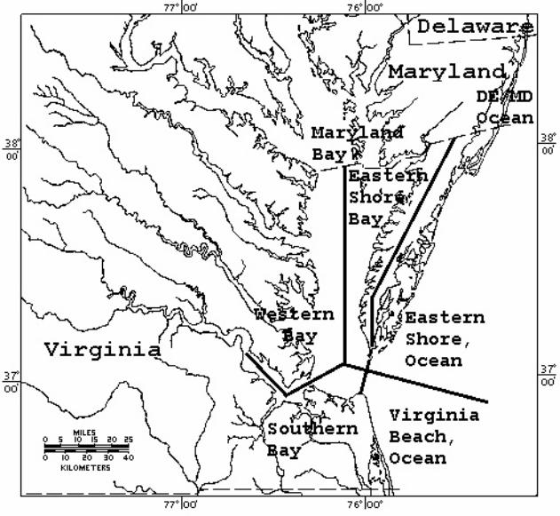
Locations of recorded strandings were grouped into 7

regions: Maryland/Delaware Ocean, Maryland Bay, Eastern Shore

Bay, Western Bay, Southern Bay, Eastern Shore Ocean and

Virginia Beach Ocean (Figure 1). Stranding frequencies were

plotted and analyzed by month and year.

14

Figure 1. Map (Mercator projection) of the lower Chesapeake

Bay and Mid-Atlantic bight, broken into 7 stranding regions:

Western Bay, Southern Bay, Virginia Beach Ocean, Eastern

Shore Ocean, Eastern Shore Bay, Maryland/Delaware Ocean and

Maryland Bay.

15

Results

The yearly number of loggerhead (Figure 2), Kemp’s

ridley (Figure 3) and leatherback (Figure 4) strandings were

plotted by year from 1979 to 1997. A simple linear

regression was computed for each species and the slope of the

regression is presented on the graphs. The slope indicates

the general state of turtle strandings (increasing,

decreasing, or constant) on a yearly basis. The graphs show

that leatherback strandings occur at a low relatively

constant rate (Figure 4) and numbers of Kemp’s ridley

strandings have been slowly increasing at a rate of about 1

turtle a year (Figure 3) since 1979. In contrast the number

of stranded loggerheads has been increasing at a rate of 3

turtles/year (Figure 2).

The bulk of the yearly loggerhead, Kemp’s ridley and

leatherback sea turtle deaths occurs in the spring of the

year (Figures 5, 6, 7) (Coles & Musick 1998). Graphs of

Kemp’s ridley (Lk) (Figure 6), loggerhead (Cc) (Figure 5)

strandings and mean water temperatures distinctly show a

primary stranding period occurring in the spring when the

water temperature approaches 21°C (Lk: s2 = 1.6) and 19°C

(Cc: s2 = 1.9) which usually occurs sometime in May. Kemp’s

ridley deaths drop to a near zero value during the middle

16

Figure 2. The number of loggerhead (Caretta caretta)

strandings in the Mid-Atlantic Bight and Chesapeake Bay by

year, from 1979 to 1997 and a simple linear regression are

plotted. The slope of the regression line is provided, and

represents a change in strandings per year. The slope

identifies an increasing trend in the state of loggerhead

deaths.

Number of Loggerhead (Caretta caretta) Deaths by Year, from 1970 to 1997.

Slope = 3.2912

70

80

90

100

110

120

130

140

150

160

170

180

190

200

210

220

230

240

250

260

79 80 81 82 83 84 85 86 87 88 89 90 91 92 93 94 95 96 97

Year

17

Figure 3. The number of Kemp’s ridley (Lepidochelys kempii)




represents a change in turtle strandings per year. The slope

identifies a general increasing trend in the state of Kemp’s

ridley deaths.

Number of Kemp's Ridley (Lepidochelys kempii) Strandings by Year, from 1979 to 1997.

Slope = 0.72R2 = 0.3753

0

5

10

15

20

25

30

35

79 80 81 82 83 84 85 86 87 88 89 90 91 92 93 94 95 96 97

Year

18

Figure 4. The number of leatherback (Dermochelys coriacea)




represents a change in turtle strandings per year. The slope

identifies a steady but slightly increasing trend in the

state of leatherback deaths.

Number of Leatherback Sea Turtle (Dermochelys coriacea) Strandings by Year,

from 1970 to 1997.

Slope = 0.45R2 = 0.61

0

2

4

6

8

10

12

14

Year

19

Figure 5. Mean number of loggerhead (Caretta caretta)

strandings (bars) and mean water temperature (oC) (line) by

week from 1979 to 1997.

Mean Number of Caretta caretta Strandings and Mean Water Temperature by Week.

0

5

10

15

20

25

0 2 4 6 8 10 12 14 16 18 20 22 24 26 28 30 32 34 36 38 40 42 44 46 48 50 52

Week

0

5

10

15

20

25

30

20

Figure 6. Mean number of Kemp’s ridley (Lepidochelys kempii)



Mean Weekly Deaths of Kemp's Ridley Sea Turtles (Lepidochelys kempii) and Mean Weekly Temperature for the Period 1979 to 1997

0

0.2

0.4

0.6

0.8

1

1.2

1.4

1.6

1.8

2

0 2 4 6 8 10 12 14 16 18 20 22 24 26 28 30 32 34 36 38 40 42 44 46 48 50 52

Week

0

5

10

15

20

25

30

21

Figure 7. Number of leatherback (Dermochelys coriacea)



Number of Leatherback Sea Turtle (Dermochelys coriacea) Strandings and Mean Water Temperature for

the Period 1979 to 1997.

0

1

2

3

4

5

6

7

8

9

1 3 5 7 9 11 13 15 17 19 21 23 25 27 29 31 33 35 37 39 41 43 45 47 49 51

Week

0

5

10

15

20

25

30

22

of the summer (Figure 6), while loggerheads maintain a low

level of strandings throughout the summer (Figure 5).

The mean water temperature for the last recorded

stranding of the year for a Kemp’s ridley is 19°C (s2 = 5.7;

Table 1, Figure 8) and for a loggerhead is 16°C (s2 = 4.4;

Table 2, Figure 9). The lag between the time turtles die and

the time they strand on the beach increases variance seen in

the estimated autumn exiting (fall, southerly migration)

water temperature. These stranding temperatures agree with

satellite sea surface temperature preferences (Coles 1998).

Leatherbacks (Figure 7) and green turtles do not occur

in sufficient numbers to determine if there are multiple

stranding peaks throughout a single season. Mean water

temperatures of first, last stranding and mean water

temperature for weeks with presence, and absence of both

leatherback (Figure 10, Table 3) and green (Table 4) turtles

were calculated. The small numbers of strandings precluded

additional analysis, because there are many years with no

strandings of either species.

VIMS sea turtle stranding data records information from

both live (usually detailed) and dead turtles. Dead turtles

were necropsied whenever possible to determine the state of

health (parasites, fat content, etc.) and the

23

Figure 8. Plot of water temperature (oC) of first (blue line)

and last (red line) stranding of Kemp’s ridley (Lepidochelys

kempii) from 1979 to 1997.

Water Temperature of First and Last Stranding Dates by Year, for Kemp's Ridley Sea Turtles

(Lepidochelys kempii).

0

2

4

6

8

10

12

14

16

18

20

22

24

26

28

30

Year

Enter Bay

Exit Bay

24

Figure 9. Plot of water temperature (oC) of first (blue line)

and last (red line) stranding of loggerhead (Caretta caretta)

from 1979 to 1997.

Water Temperature of First and Last Stranding Dates by Year, for Loggerhead Sea Turtles (Caretta caretta).

0

5

10

15

20

25

30

Year

Enter Bay

Exit Bay

25

Figure 10. Plot of water temperature (oC) of first (blue

line) and last (red line) stranding of leatherback

(Dermochelys coriacea) from 1979 to 1997.

Water Temperatures of First and Last Stranding Dates by Year, for Leatherback Sea Turtles

(Dermochelys coriacea).

0

5

10

15

20

25

30

Year

Enter Bay

Exit Bay

26

cause of death. Despite the attempts to determine the cause

of death, the cause could not be determined in a majority of

stranded turtles because of the advanced state of

decomposition (Table 5). A significant number of the total

records came from live turtles that were recovered from pound

nets. There are no identifiable trends in the cause of death

data for loggerheads, Kemp’s ridleys or leatherbacks, in part

due to the lack of detailed cause of death data.

Almost all the turtles recovered (live or dead) were

juveniles, determined by carapace length and/or internal

exam. There was no size frequency shift in loggerhead

strandings between months (Figure 11) or years (Figure 12).

Each month and year had a similar distribution of stranding

lengths. Kemp’s ridleys on the other hand showed a length

frequency shift from small to large turtles as the season

progressed (Figure 13), although there was no pattern of

length frequency changes between years (Figure 14). There

was insufficient data to draw any conclusions for green or

leatherback turtles.

All the verified strandings in the VIMS data base were

grouped into 7 regions: Maryland & Delaware Ocean (MDO),

Maryland Bay (MB), Eastern Shore Bay (ESB), Western Bay (WB),

Southern Bay (SB), Eastern Shore Ocean (ESO) and

27

Figure 11. Tip to Tip (T-T) length frequency graph of

loggerhead sea turtles (Caretta caretta) by month for the

years 1979, 1980, 1987-1997.

Frequency of Loggerhead (Caretta caretta) Strandings by Size Class and Month.

0

25

50

75

100

125

150

175

200

225

250

275

300

Curved Carapace (T-T) Length (cm)

Jan

Feb

Mar

Apr

May

Jun

Jul

Aug

Sep

Oct

Nov

Dec

28

Figure 12. Tip to Tip (T-T) length frequency graph of

loggerhead sea turtles (Caretta caretta) by year.

Frequency of Loggerhead (Caretta caretta) Strandings by Size Class and Year

0

10

20

30

40

50

60

70

80

90


79

80

87

88

89

90

91

92

93

94

95

96

97

29

Figure 13. Tip to Tip (T-T) length frequency graph of Kemp’s

ridley sea turtles (Lepidochelys kempii) by month for the

years 1979, 1980, 1987-1997.

Frequency of Kemp's Ridley (Lepidochelys kempii) Strandings by Size Class and Month.

0

5

10

15

20

25

30

0-10 10.1-20 20.1-30 30.1-40 40.1-50 50.1-60 60.1-70 >70.1


Jan

Feb

Mar

Apr

May

Jun

Jul

Aug

Sep

Oct

Nov

Dec

30

Figure 14. Tip to Tip (T-T) length frequency graph of Kemp’s

ridley sea turtles (Lepidochelys kempii) by year.

Frequency of Kemp's Ridley (Lepidochelys kempii) Strandings by Size Class and Year.

0

1

2

3

4

5

6

7

8

9

10

11

0-10 10.1-20 20.1-30 30.1-40 40.1-50 50.1-60 60.1-70 >70.1


79

80

87

88

90

91

92

93

94

95

96

97

31

Virginia Beach Ocean (VBO) (Figure 1). The trends in

loggerhead stranding location viewed by year (Figure 15) show

a steadily increasing number of deaths in all areas in recent

years. Similar trends are seen for Kemp’s ridleys

(Figure 16). Loggerhead and Kemp’s ridley data show

particularly high yearly stranding numbers in the SB and VBO

regions. Stranding frequencies by month clearly show that

strandings peak in all regions in June, and that VBO also has

a fall (October) peak (Figures 17, 18) (large for Kemp’s

ridleys, and small for loggerheads). The large June peak

corresponds to the water temperature increase that occurs as

the turtles migrate into the Bay. The fall VBO peaks

correspond to times the turtles are migrating out of the Bay.

Leatherback and green turtle deaths do not occur in

sufficient numbers to determine yearly or monthly trends.

They tend to strand in the same areas, SB, WB and VBO, as the

loggerheads and Kemp’s ridleys (Figure 19). The lack of

Kemp’s ridley turtles in the MDB and MD/DE regions is due to

the lack of awareness and any semblance of a sea turtle

stranding program until the mid 90’s.

32

Figure 15. Frequency of loggerhead sea turtle (Caretta

caretta) strandings by location and year.

Stranding Locations of Loggerhead Sea Turtles (Caretta caretta) by Year

0

10

20

30

40

50

60

70

MD/DE Ocean MD Bay Eastern Shore,Bay

Western Bay Southern Bay Eastern Shore,Ocean

VA BeachOcean

Stranding Location by Year

798087889091929394959697

33

Figure 16. Frequency of Kemp’s ridley sea turtle

(Lepidochelys kempii) strandings by location and year.

Stranding Locations of Kemp's Ridley Sea Turtles (Lepidochelys kempii) by Year.

0

2

4

6

8

10

12

14

MD/DE, Ocean MD, Bay Eastern Shore,Bay


VA Beach, Ocean

Stranding Location by Year

79

80

87

88

90

91

92

93

94

95

96

97

34

Figure 17. Frequency of loggerhead sea turtle (Caretta

caretta) strandings by location and month for the years 1979,

1980, 1987-1997.

Stranding Locations of Loggerhead Sea Turtles (Caretta caretta) by Month.

0

50

100

150

200

250

300

MD/DE Ocean MD Bay Eastern Shore,Bay


VA Beach Ocean

Location of Stranding by Month

Jan

Feb

Mar

Apr

May

Jun

Jul

Aug

Sep

Oct

Nov

Dec

35

Figure 18. Frequency of Kemp’s ridley sea turtle

(Lepidochelys kempii) strandings by location and month for

the years 1979, 1980, 1987-1997.

Stranding Locations of Kemp's Ridley Sea Turtles (Lepidochelys kempii) by Month

0

2

4

6

8

10

12

14

16

18

20

22

24

26

28



VA Beach, Ocean

Stranding Location by Month

Jan

Feb

Mar

Apr

May

Jun

Jul

Aug

Sep

Oct

Nov

Dec

36

Figure 19. Frequency of leatherback sea turtle (Dermochelys

coriacea) strandings by location for the years 1979, 1980,

1987-1997.

Frequency of Leatherback (Dermochelys coriacea) Strandings by Location.

0

5

10

15

20

25



VA Beach, Ocean

Stranding Location

37

Discussion

Due to the nature of the data collected, we can only

make broad generalizations about many of the trends

identified. One problem with the data set is spatial

discrepancies of effort in reporting turtle strandings

because beaches are not equally patrolled (marshy areas

receive less coverage than broad sandy beaches).

Additionally stranding coverage was more complete in some

years than others because of fluctuations in the availability

of resources and funds (low funds or resources makes for low

numbers of records). In many cases the only information

recorded was the date that a dead turtle was reported, unless

there was a good chance the turtle was a Kemp’s ridley or

leatherback, species were not determined. As a result some

general trends may be identified, but specific nuances may

remain hidden.

The identification number assigned to stranded turtles

represents the discovery date, not the date of death. Death

may have occurred days or even weeks prior to discovery (a

newly dead turtle will tend to sink; as it decomposes the gas

produced will cause the turtle to float; floating turtles are

then blown ashore). This accounts for the spurious sightings

of turtles during the fall and winter, when water

temperatures are well below that of the lethal minimum

temperature (decomposition takes longer).

The driving force behind the large yearly fluctuations

in stranding numbers (Figures 2, 3, 4) make the trend line at

38

best a simple first order approximation. The fluctuations

may be driven by multiple factors including fishing

mortality, recreational boat interactions, water temperature,

or other unidentified environmental factors and stranding

coverage.

One of the major factors determining the presence of sea

turtles in the Bay is water temperature. As the water

temperature approaches 20oC turtles start to enter the Bay.

The mean weekly stranding numbers of loggerhead (Figure 5),

Kemp’s ridley (Figure 6) and leatherback (Figure 7) sea

turtles show that most of the years’ strandings come in the

spring, when the turtles first enter the Bay. It is not

surprising that the weekly water temperature means with

turtles (loggerhead, t0.05(1)941 = 12.14; Kemp’s ridley,

t0.05(1)941 = 2.33; where nomenclature for t is probability of a

Type 1 error, 1 or 2 tailed test, degrees of freedom n-2) are

significantly higher than those weekly means without turtles

(Tables 1, 2, 3). Although the magnitude of the water

temperature doesn’t correlate with the total numbers of

turtles in the Bay there is a threshold temperature, 20oC,

which is a signal that can be easily monitored. The plots of

water temperature for first and last strandings of the year

(Figures 10, 11, 12) clearly supports our temperature

findings.

Many sea turtles entering the Bay early in the spring

are in poor health, emaciated and heavily encrusted with

Chelonibia barnacles (Belmund 1988, Bellmund et al. 1987,

39

Lutcavage & Musick 1985). These compromised turtles enter

the Chesapeake Bay early in the season and in a

physiologically weakened state. A sharp thermal lens exists

in the Bay until late spring, which keep the turtles in the

upper water column, away from benthic food sources. The

delay in feeding further depletes the turtle’s energy

reserves. In this weakened state, turtles may confine their

activities to the warm surface water until the thermal lens

has broken down, making benthic food sources available.

In the 1870’s, fishing techniques significantly changed

as pound nets were introduced to the Chesapeake Bay (Reid

1955). The pound and other nets can entangle and drown

physiologically weakened turtles (later in the year when

turtles have replenished their energy reserves, they are

better able to avoid pound nets) (Bellmund et al. 1987, Byles

1988, Musick 1995, Musick et al. 1985, Lutcavage & Musick

1985). More recently, recreational fishing and boating has

increased. The increase of boat traffic and recreational

fishing in the spring (fish, as well as turtles, migrate into

the bay) increases the number of interactions with turtles.

The turtles’ natural avoidance response to aerial or surface

stimulus is to dive (Wyneken et al. 1994). If a thermal lens

is present, turtles maybe forced through it, cooling the

body. Reducing the body core temperature further

physiologically compromises the turtle. These cold turtles

which are less active may drift into nets, become entangled

and drown. Turtles that arrive later in the spring enter an

40

environment where food is immediately available (thermal lens

has dissipated). They can quickly replenish their energy

reserves and are able to avoid nets (Bellmund et al. 1987).

Loggerheads and Kemp’s ridleys have different stranding

patterns (Figures 5, 6). This difference is reflected in the

different habitat types the turtles use during the summer.

Kemp’s ridleys are generally found in shallow, less than 5

meters depth, protected grass beds, and are removed from most

commercial fishing activities. Loggerheads utilize the edges

of channels in water depths of 5 to 13 meters (Byles 1988,

Musick 1988, Musick & Limpus 1997). The loggerheads are

exposed to more anthropogenic interactions than Kemp’s

ridleys, which account for the larger number of loggerhead

strandings during the midsummer.

In the fall as the Kemp’s ridleys start to migrate out

of the Bay there is a second, smaller stranding peak

(Figure 6) presumably due to the turtles reentering areas

where the number of human interactions increases. It is

clear that to reduce Kemp’s ridley mortality in Virginia,

efforts should focus on the spring and fall migration

periods. The Kemp’s ridleys do not seem to be particularly

susceptible to fishing or other stresses while feeding in the

Bay. Loggerhead strandings do not exhibit this secondary

peak; stranding numbers just dwindle to zero as the water

temperature drops. Leatherback stranding numbers exhibit a

large spring peak, with a fall peak as well, although the

41

numbers are too small to draw definitive conclusions

(Figure 7).

The causes of sea turtle mortality previously identified

by Lutcavage (1981) are: Pound net entanglement, boat or

propeller damage, haul seine, long line, rod and reel,

mutilation, crab pot entanglement and natural predation. The

present data set lumped these into commercial fishing

(Net/crab line entanglement), boat/propeller, hook & line

fishing, malicious mutilation, and natural causes (predation

& illness) (Table 5). In 1980 at least 30% of the stranded

turtles died due to pound net hedging entanglement, and it is

likely that more turtles were tangled and drowned than were

reported (Lutcavage 1981). However the percentage of net

related deaths for the period 1979-1983 was only 18.6

(Bellmund et al. 1987). In contrast there are only 2.4%

confirmed entanglements of loggerhead turtles throughout the

whole period (Table 5). This suggests that there was a

change in techniques used to identify entangled turtles. It

is likely that entanglement deaths are and have been vastly

underreported, in part because the turtles have decomposed

beyond the point that a cause of death can be determined at

the time of discovery and regular surveys of sea turtles

entangled in nets have been discontinued. The general

consensus remains that commercial fishing has a great

influence on the numbers of sea turtle deaths (Coles & Musick

1998, Terwilliger & Musick 1995), although the cause of death

for the vast majority of strandings is unknown.

42

Previous studies have shown that sub adult turtles are

the preponderant size class in the Bay (Lutcavage 1981,

Byles 1988). If we make the assumption that turtle strandings

represent a random sample of the population, then these

stranding results support those conclusions,

(Figures 14, 16). The loggerhead population structure of the

is uniform both annually and inter-annually (Figure 13, 14)

with a majority of the loggerheads being in the 50-80 cm

range. The Kemp’s ridley population does not show the same

pattern. The monthly standing data show unexplained shifts

in the turtle’s population structure as the year progresses

(June-Sept.) (Figure 15). It is possible that this pattern

is due to random perturbations in the total number because of

the small number of Kemp’s ridleys recorded on a yearly basis

(Figure 16). Therefore the strandings in an individual year

can have a large influence on monthly trends. Chesapeake Bay

loggerheads come from multiple nesting populations

(Norrgard 1995). These nesting areas cover a vast geographic

region along the Atlantic coast, from Virginia to Florida.

The large numbers and distribution of loggerheads decreases

the effects of random perturbations, or the lack of hatchling

success from a single local event on an individual beach.

All the verified strandings in the VIMS data base were

grouped into 7 regions: Maryland & Delaware Ocean (MDO),

Maryland Bay (MB), Eastern Shore Bay (ESB), Western Bay (WB),

Southern Bay (SB), Eastern Shore Ocean (ESO) and Virginia

Beach Ocean (VBO) (Figure 1). Loggerhead and Kemp’s ridley

43

data show high yearly stranding numbers in the SB and VBO

regions. The higher stranding numbers from SB and VBO

possibly represent spatial discrepancies in reporting effort,

because all beaches are not patrolled equally. The SB and

VBO are primarily areas with wide sandy beaches, heavily used

by both local residence and tourists (especially when turtles

are present). Other areas of the coast are not uniformly

covered. Large areas are not easily accessible, even by boat

(mud flat and marsh), and so are not regularly patrolled, if

at all. The Eastern Shore has the least consistent coverage

of any region, which is reflected in the low stranding

numbers. Maryland numbers are low because they do not have

the same number of turtles in their region as is seen in the

lower Bay, and their coverage is sporadic like most of the

marshy areas in the Bay.

Recently there has been a large increase in the number

of strandings in the SB, the beaches of Fisherman’s Island,

Kiptopeke State Park and Sunset Beach areas of Northampton

County. It is likely that this increase is due to an

increase in commercial fishing, particularly the spring gill

net fisheries, where large meshed gill nets are used

(Terwilliger and Musick 1995). Although since 1995 there has

been a dramatic increase in boat traffic due to the

construction of the new Chesapeake Bay Bridge Tunnel (CBBT)

span from Fisherman’s Island to the north (CBBT) tunnel

island.

44

This study of sea turtle stranding data demonstrates

several major points. 1) Juvenile sea turtles enter and

utilize the Chesapeake Bay as a feeding area when the water

temperature approaches 20oC, and they leave after the water

temperature drops below 20oC. 2) The cause of death

attributed to the largest number of strandings is boat and

propeller damage because such damage is easy to recognize.

Interactions (entanglement) with commercial fishing gear were

second in importance, but such interactions, while usually

resulting in turtles drowning, may be less apparent. The

vast bulk of the strandings are of unknown cause of death due

to decomposition and lack of observer training. 3) The size

composition of loggerheads in the Bay is uniform both between

and within years. Kemp’s ridleys show a lot more variation

in their size composition within and between years. Analysis

of this data has re-enforced the importance of uninterrupted

support for long-term monitoring projects. In addition,

detailed data on the location of fishing effort and

seasonality is needed to test for correlations between

fishing activities and sea turtle strandings.

45

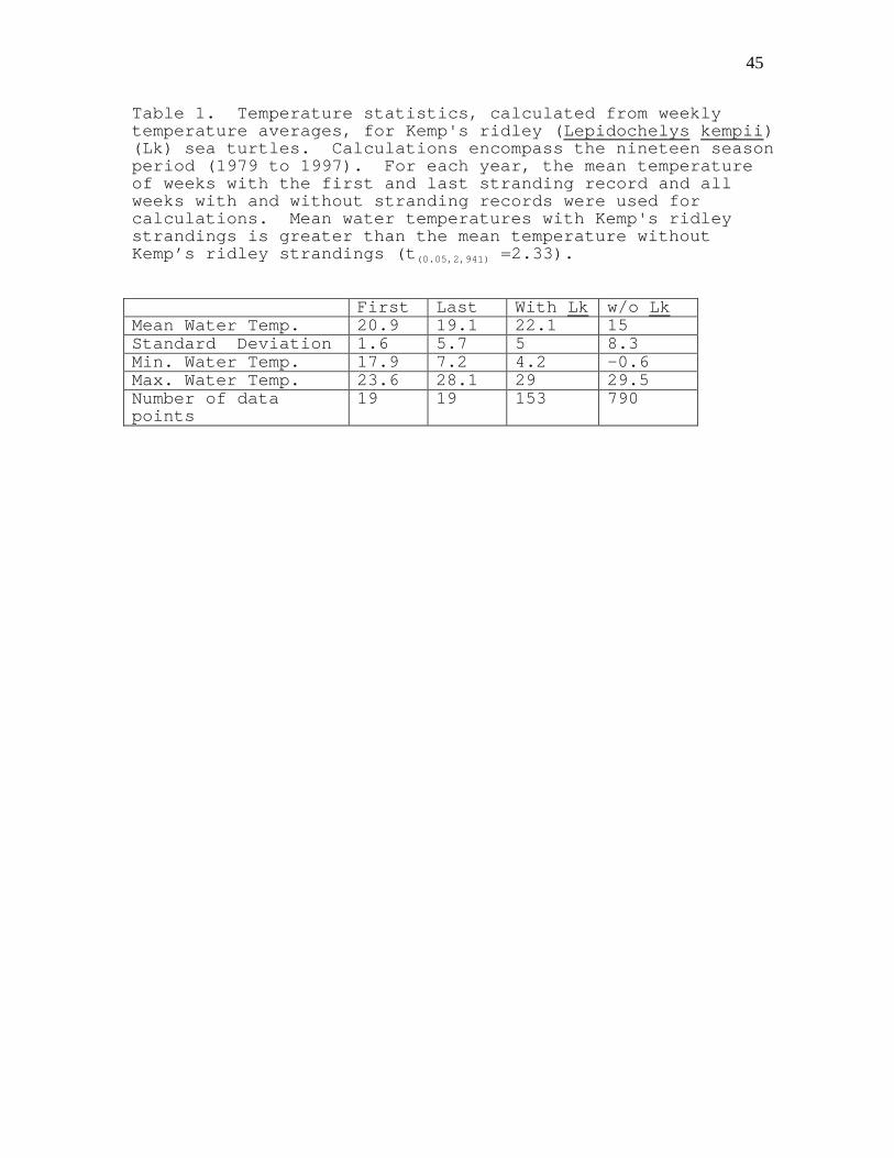
Table 1. Temperature statistics, calculated from weeklytemperature averages, for Kemp's ridley (Lepidochelys kempii)(Lk) sea turtles. Calculations encompass the nineteen seasonperiod (1979 to 1997). For each year, the mean temperatureof weeks with the first and last stranding record and allweeks with and without stranding records were used forcalculations. Mean water temperatures with Kemp's ridleystrandings is greater than the mean temperature withoutKemp’s ridley strandings (t(0.05,2,941) =2.33).

First Last With Lk w/o LkMean Water Temp. 20.9 19.1 22.1 15Standard Deviation 1.6 5.7 5 8.3Min. Water Temp. 17.9 7.2 4.2 -0.6Max. Water Temp. 23.6 28.1 29 29.5Number of datapoints

19 19 153 790

46

Table 2. Temperature statistics, calculated from weeklytemperature averages, for loggerhead (Caretta caretta) seaturtles (Cc). Calculations encompass the nineteen seasonperiod (1979 to 1997). For each year, the mean temperatureof weeks of the first and last stranding record and all weekswith and without stranding records were used forcalculations. The mean water temperature with Loggerheads issignificantly higher than the water temperature withoutloggerheads (t0.05,(1),941 = 12.14).

First Last With Cc w/o CcMean Water Temp. 18.7 15.7 21.5 10.5Standard Deviation 1.9 4.4 6.2 6.2Min. Water Temp. 15.3 10.8 -0.6 0.5Max. Water Temp. 22.5 26.9 29.5 28.5Number of datapoints

19 19 483 460

47

Table 3. Temperature statistics, calculated from weeklytemperature averages, for leatherback (Dermochelys coriacea)sea turtles (Dc). Calculations encompass the nineteen seasonperiod (1979 to 1997). For each year, the mean temperatureof weeks of the first and last stranding record and all weekswith and without stranding records were used forcalculations. There was insufficient data to meaningfullycompare temperatures.

First Last With Dc w/o DcMean Water Temp. 22.9 21.6 23.6 15.6Standard Deviation 2.6 6.1 3.99 8.3Min. Water Temp. 18.4 10.7 10.7 -0.6Max. Water Temp. 27.4 27.6 28.6 29.5Number of datapoints

17 16 66 877

48

Table 4. Temperature statistics, calculated from weeklytemperature averages, for green (Chelonia mydas) sea turtles(Cm). Calculations encompass the nineteen season period(1979 to 1997). For each year, the mean temperature of weeksof the first and last stranding record and all weeks withgreen turtle and without green turtle stranding records wereused for calculations. There was insufficient data tomeaningfully compare temperatures.

First Last With Cm w/o CmMean Water Temp. 23.5 13.3 19.5 15.3Standard Deviation 3.4 5.2 5.5 8.8Min. Water Temp. 18.1 6.4 6.4 -0.6Max. Water Temp. 27.3 20.9 27.3 29.5Number of datapoints

9 6 22 966

49

Table 5. Frequency of sea turtle strandings lumped by causeof mortality. The data represents a total for years 1979,1980, 1987, 1988, and 1990-1997. Loggerhead (Carettacaretta) (Cc), Kemp’s ridley (Lepidochelys kempii) (Lk), andleatherback (Dermochelys coriacea) (Dc) data are presented.With the exception of live and sick turtles recovered(primarily from pound nets) the data represents turtlemortality. The causes of sea turtle mortality identified byLutcavage (1981) were lumped into commercial fishing(net/crab line entanglement), boat/ propeller, hook & linefishing, malicious mutilation (hammer, knife, gunshot) andillness or natural causes.

Cc Lk DcMissing/Unknown 1443 111 34Boat/Propeller 157 5 13Entanglement 49 6 5Hook & Line 3 0 0Malicious 27 0 0Illness/Natural 41 3 0Live, IncidentalCapture

358 57 2

50

Literature Cited

Bellmund, S.A., J.A. Musick, R.E.C. Klinger, R.A. Byles, J.A.

Keinath, D.E. Barnard. 1987. Ecology of Sea Turtles in

Virginia, Special Scientific Report No. 119, Virginia

Institute of Marine Science, College of William and Mary,

Gloucester Point, VA, 23062. 48p.

Byles, R.A. 1988. Behavior and ecology of sea turtles from

Chesapeake Bay, Virginia. Unpublished Dissertation. School

of Marine Science, Virginia Institute of Marine Science,

College of William & Mary, Gloucester Point, VA.

Coles, W.C. & J.A. Musick. 1998. Record numbers of sea

turtle strandings in Virginia in May and June 1998.

Virginia Marine Resource Report Number 98-4. Virginia

Institute of Marine Science, Gloucester Point, VA.

Lutcavage, M. 1981. The status of marine turtles in

Chesapeake Bay and Virginia coastal waters. Unpublished

Thesis. School of Marine Science, Virginia Institute of

Marine Science, College of William & Mary, Gloucester

Point, VA.

Lutcavage, M. & J.A. Musick. 1985. Aspects of the Biology of

Sea Turtles in Virginia. Copiea 2:449-456.

Musick , J.A. & C.J. Limpus. 1997. Habitat utilization in

Juvenile Sea Turtles. IN Lutz, P.L. and J.A. Musick.

1997. The Biology of Sea Turtles. CRC Press, New York,

NY.

Musick, J.A. 1995. Interactions of Fisheries with Sea

Turtles and Marine Mammals in Virginia. Proceedings of the

51

Workshop on the Management of Protected Species/Fisheries

Interactions in State Waters. Atlantic States Marine

Fisheries Commission Spec. Rept. 54:74-83.

Musick, J.A. 1988. The Sea Turtles of Virginia. Virginia

Sea Grant Communications Office, Virginia Institute of

Marine Science, Gloucester Point, VA. 22pp.

Norrgard, J. 1995. Determination of stock composition and

natal origin of a juvenile loggerhead turtle population

(Caretta caretta) in Chesapeake Bay using mitochondrial DNA

analysis. . Unpublished Thesis. School of Marine Science,

Virginia Institute of Marine Science, College of William &

Mary, Gloucester Point, VA.

Reid, George K., Jr. 1955. The Pound net fishery in

Virginia. Part 1 - History, Gear Description, and Catch.

Commercial Fisheries Review 17(5):1-15.

Terwilliger, K. and J.A. Musick (co-chairs), Virginia Sea

Turtle and Marine Mammal Conservation Team. 1995.

Management Plan for Sea Turtles and Marine Mammals in

Virginia, Final Report to the National Oceanic and

Atmospheric Administration. 56pp.

Virginia Institute of Marine Science 1997. Marine Turtle Data

Data. Scientific Data Archive, Va. Institute of Marine

Science, School of Marine Science, College of William &

Mary. Gloucester Pt., VA 23062

Virginia Institute of Marine Science. current_month, 1995.

York River Ambient Monitoring Data. VIMS Scientific Data

Archive (http://www.vims.edu/data_archive). Va. Institute

52

of Marine Science, School of Marine Science, College of

William & Mary. Gloucester Pt., VA 23062

Virginia Marine Resources Commission 1996. Yearly Commercial

Fishing Landings Data.

Virginia Marine Resources Commission 1996. Yearly Commercial

Fishing License Data.

Wyneken, J., M. Goff, L. Glenn. 1994. The trials and

tribulations of swimming in the near-shore environment.

IN: Bjorndal, K.A., A.B. Bolten, D.A. Johnson, and P.J.

Eliazar (Compilers). Proceedings of the Fourteenth Annual

Symposium on Sea Turtle Biology and Conservation. NOAA

Technical Memorandum NMFS-SEFSC-351, pp169-171.

Zar, J.H. 1984. Biostatistical Analysis. Prentice-Hall,

Inc. Englewood Cliffs, NJ.

53

Morphometrics of Sea Turtles in Virginia.

54

Introduction

Anatomical measurements have been made on stranded and

live Kemp’s ridley (Lepidochelys kempii) and loggerhead

(Caretta caretta) sea turtles in the Commonwealth of Virginia

since 1979. Often stranded turtles are disarticulated,

pieces are missing, or the turtle’s position, condition,

location make measurements unreliable or impossible.

Occasionally the only piece of the turtle that can be

reliably measured is the head. Often there is a need to

accurately convert between one or more measurements for

various biological and physical analyses.

The objective of this study is to provide a morphometric

analysis of loggerhead and Kemp’s ridley sea turtles from

Virginia and provide regression equations to allow for

conversion from one kind of measurement to another.

55

Materials and Methods

Since 1979, measurements of stranded sea turtles found

in Virginian waters, have been made by members of the

Virginian sea turtle stranding network. Straight

measurements (S) were made with either one or two meter

calipers, curved measurements (C) were made with fibrous

measuring tapes. All measurements were made by trained

volunteers and recorded on the Virginia Institute of Marine

Science (VIMS) sea turtle stranding forms.

Carapace measurements taken are: Notch to Notch (NN),

Tip to Tip (TT), Width (CW) and Notch to Tip (NT). The NT

measurement was only recently added to fulfill a National

Marine Fisheries Service (NMFS) sea turtle stranding network

requirement. Head length (HL) and head width (HW)

measurements are also made (Figure 1). Plastron measurements

are taken when available (width without bridge (PW), width

with bridge (PWB), and length (PL)) (Figure 2). Carapace

lengths and widths are made to the marginal edge of the

carapace and recorded as both curved (C) and straight (S)

measurements. Straight measurements require that observers

have calipers, which are not available to all volunteer

observers, and are frequently not recorded. All plastron and

head measurements are made with calipers making them the

least

56

Figure 1. Line drawing of the carapace of a marine turtle,

showing the location of carapace and head measurements made.

The measurements are: (TT) - Tip to Tip, (NT) - Notch to Tip,

(NN) - Notch to Notch, (HL) - Head Length, (HW) - Head Width

and W - Carapace Width.

57

Figure 2. Line drawing of the plastron of a marine turtle,

showing the location of plastron measurements made. The

measurements are: (PW) - Plastron width, without Bridge,

(PWB) - Plastron Width with Bridge and (PL) - Plastron

Length.

58

frequent measurements recorded. Curved measurements are

simply made with a tape measure and are the most frequent

measurements recorded. These data were entered into a

Microsoft Access™ database and all data used for analysis

were checked with original data sheets. Forty-eight

loggerhead hatchling measurements were provided from a study

of loggerhead nesting parameters (Jones, W. 1997. Personal

Communication. Hatchling sea turtle data. Virginia Institute

of Marine Science, Gloucester Point, VA).

Weight estimates are generally derived from a

corresponding volume measure, generalized as length cubed,

(l3), of the organism (Schmidt-Nielsen 1985, Calder 1984).

Turtle lengths and widths are reliable measurements. Turtle

depth (dorso-ventral length) is not recorded. Rapid

decomposition after death and bloating also make turtle

height an unreliable measurement. This makes the l3 estimate

for weight inappropriate.

The shape, curvature, of the carapace (how domed it is)

should be a good indicator of the weight of the turtle.

Curvature (k) is generally defined as ∂θ/∂s (change of angle

(θ) divided by the change of arc length (s)). By observation

of the cross section shape of the carapace we assume that the

first order curvature of the sea turtles carapace can be

approximated as a circle. That circle can be defined by the

arc (curved carapace width) and chord (straight carapace

width). The radius (r) of the circle and angle (described by

the arc and chord) can be numerically solved from the

59

relationship arc/chord = (r*θ)/(r*sin(θ)). Conveniently,

circles have constant curvature, which simplifies the

equation for curvature to k = 1/r (Shenk, 1984). The

curvature was regressed against weight and curved notch to

notch carapace length for loggerheads and Kemp’s ridleys.

For each regression, the original data set was sorted

and filtered to eliminate unknown, unreliable species

identification and unpaired data. Simple linear regressions

for lengths and widths for loggerheads and Kemp’s ridley sea

turtles were calculated for all measurement combinations.

The significance of regression coefficients were tested with

F-tests (α = 0.05) (Zar 1984).

60

Results and Discussion

Morphological measurements made on vertebrates generally

involve measurements along the long and occasionally the

short axis of the structure (Hall 1962). By consistently

taking these measurements we are able to provide estimates

and corrections for missing and suspicious data.

Linear regression equations, coefficient of

determination (r2) sample sizes, and F-test are shown for

Kemp’s ridleys (Table 1) and loggerhead (Table 2). The high

coefficient of determination (r2, an indication of the

accuracy of the predictions) shows that most of the variation

in turtle measurements is dependent on the size of the

turtle. This makes these regression equations excellent

estimators for erroneous and missing measurements. The high

coefficient of determination of these regressions is similar

to those presented for green turtles (Chelonia mydas)

(Bjorndal and Bolten 1989).

All linear regressions were found to be significant

(α = 0.05). From scatter plots and regression equations of

Kemp’s ridley or loggerhead sea turtles (Table 1, 2), there

is only one morphological population, of each species,

present in Virginian waters. This is expected for Kemp’s

ridleys because they all come from the same breeding

population (The entire population of Kemp’s ridleys nest in

one restricted area (Rancho Nuevo) in Tamaulipas, Mexico),

making them a truly panmictic species.

61

Virginian loggerhead sea turtles come from two

populations, as determined by mitochondrial DNA analysis

(Norrgard 1995), 58% from the Georgia/South Carolina nesting

populations and 42% from the Florida nesting population.

There are no distinguishing morphological features seen in

our data set.

The greatest variability (lowest r2) occurred for the

linear regressions involving head measurements. Allometric

equations (y = a * xb, or log(y) = log(a) + b*log(x)) have two

important terms, a- the intercept at unity, and b- slope of

the regression line. Customarily the original data is log

transformed to handle biological scaling problems (Schmidt-

Nielsen 1985, Calder 1984, Vogel 1988). In most cases the r2

accounted for over 90% of the variability. The cases of

lower r2 the power transformation did not appreciably improve

the values. Although this wasn’t unexpected for the carapace

and plastron comparisons, the carapace head measurements were

also linear. Most of the variation may be explained by

differences in individual measurer’s techniques. Carapace

measurements are explicit, because measurements are made to

the marginal edge of the shell. Head measurements are more

subjective, requiring a familiarity of cranial anatomy, and

experience, making cranial measurements more subject to

observer bias.

Curvature of the carapace was calculated for loggerheads

and Kemp’s ridleys. The curvature was plotted against weight

(Figure 3), and the curved carapace length (notch to notch)

62

was plotted against curvature (Figure 4). These plots all

exhibited significant power relationships for the

loggerheads, and highly significant for the Kemp’s ridleys.

The high r2 for the curvature-weight estimates show that using

curvature to estimate weight (Figure 3) is as good as

carapace length (Figure 5).

A turtle’s carapace changes shape as it grows; which is

seen as a decrease in the curvature of the carapace as the

length increases (Figure 4). The decrease in curvature may

be correlated to the increase in swimming speed as the turtle

grows (Wyneken 1997). The faster the turtle swims, the

greater the lift created by a highly domed carapace.

Therefore the turtles carapace likely changes shape in order

to optimize lift and drag for the turtle’s “cruising”

velocity. Wind tunnel/flow tank studies of the lift and drag

of different carapace shapes will validate these preliminary

numbers.

63

Figure 3. Scatter plot, trendline and allometric scaling

equations of curvature and weight for loggerhead (Caretta

caretta) (a) and Kemp’s ridley (Lepidochelys kempii) (b) sea

turtles. The coefficient of determination (r2) for the

equations and number of data points are also presented.

Kemp's Ridley (Lepidochelys kempii), Curvature vs. Weight.

y = 0.0009x-2.3579

R2 = 0.9094N = 81

0

5

10

15

20

25

30

35

40

45

50

0.00 0.01 0.02 0.03 0.04 0.05

Curvature

Loggerhead (Caretta caretta), Curvature vs. Weight.

y = 0.0002x-2.9283R2 = 0.8319N = 415

0

20

40

60

80

100

120

140

160

0 0.005 0.01 0.015 0.02 0.025 0.03

Curvature

64


equations of carapace length (notch to notch) and curvature

for loggerhead (Caretta caretta) (a) and Kemp’s ridley

(Lepidochelys kempii) (b) sea turtles. The coefficient of

determination (r2) for the equations and number of data points

are also presented.

Loggerhead (Caretta caretta), Carapace Length vs Curvature

y = 0.5469x-0.8273R2 = 0.71N = 624

0

0.005

0.01

0.015

0.02

0.025

0.03

0.035

0.04

0.045

0.05

0 10 20 30 40 50 60 70 80 90 100 110 120 130

Curved Carapace (N-N) Length (cm)

Kemp's Ridley (Lepidochelys kempii), Carapace Length vs. Curvature.

y = 1.9949x-1.2278

R2 = 0.9274N = 102

0.00

0.01

0.02

0.03

0.04

0.05

0.06

0 20 40 60 80


65


equations of carapace length (notch to notch) and weight for

loggerhead (Caretta caretta) (a) and Kemp’s ridley

(Lepidochelys kempii) (b) sea turtles. The coefficient of

determination (r2) for the equations and number of data points

are also presented.

Kemp's Ridley (Lepidochelys kempii), Carapace Length vs. Weight.

y = 9E-05x3.0786

R2 = 0.9525N = 79

0

5

10

15

20

25

30

35

40

45

50

0 10 20 30 40 50 60 70 80


Loggerhead (Caretta caretta), Carapace Length vs. Weight.

y = 0.0004x2.7108R2 = 0.9136N = 415

0

20

40

60

80

100

120

140

160

180

0 20 40 60 80 100 120


66

Without data from lift and drag experiments we can

identify certain traits of the turtle as it moves through the

water. These can be determined by looking at the Reynolds

number (Re), which is “the nearest thing to a completely

general guide to what is likely to happen when a solid and a

fluid encounter each other” (Vogel 1989). The Reynolds number

is a non-dimensional number representing the ratio of

inertial and viscous forces and is the index from which

different flows can be compared.

Hatchling and juvenile sea turtles live in a world of

moderate Re, ranging from 1.1 x 104 to 4.6 x 104 (Wyneken

1988, 1997). Reynolds numbers were calculated from mean sea

water density and viscosity values, Virginian loggerhead

turtle lengths and swimming speeds from Wyneken (1997).

These values ranged from (1.17 x 104 to 1.57 x 104) for

hatchlings to (1.9 x 104 to 3 x 105) for migrating adults.

The turtle’s operate at a lower Re than calculated for many

other migratory species (Wyneken 1997, Vogel 1981). This low

number may be a result of the turtle’s ectothermic

physiology, not being able to maintain elevated metabolic

rates. The turtles may compromise for the low efficiency by

increasing their apparent lift by the curvature of the

carapace.

It is apparent that the analyses provided herein may

provide a useful tool for the study of physical and

mechanical aspects of sea turtle biology. The regression

67

equations may be used to accurately estimate measurements

that are missing or to check for errors in data sets.

68

Acknowledgments

This project was funded, in part, by the Virginia

Coastal Resources Management Program of the Department of

Environmental Quality through Grant # NA37O00287-01 of the

National Oceanic and Atmospheric Administration, Office of

Ocean and Coastal Resource Management, under the Coastal Zone

Management Act of 1972, as amended. Parts of this project

were funded by Virginia Game and Inland Fish-Non Game

Program. Thanks are due to all the past and present

volunteers who assisted in collecting and maintaining the

Virginia sea turtle stranding data.

69

Table 1. Linear regressions of Kemp’s ridley (Lepidochelyskempi) sea turtle measurements, from VIMS stranding data.Comparisons of; straight (S) and curved (C) carapace [notchto notch (NN), tip to tip (TT), notch to tip (NT) and width(W)] plastron [width (PW), width with bridge (PWB) and length(PL)] and head [length (HL) and Width (HW)], measurements areshown with the respective r2, N and F values.

Equation r2 N FS:NT = (1.0114 * S:NN) + 0.1091 0.9995 33 64901.9S:NT = (0.9894 * S:TT) - 0.0853 0.9994 33 50483.5S:NT = (1.0548 * S:W) + 0.885 0.9794 33 1475.8S:NT = (1.7944 * PW) - 0.7996 0.9560 30 608.3S:NT = (1.2971 * PWB) 1.8584 0.9603 31 701.9S:NT = (1.3485 * PL) - 1.4587 0.9929 31 4078.4S:NT = (0.9645 * C:NT) - 0.6732 0.9964 29 7577.4S:NT = (0.9723 * C:NN) - 0.6629 0.9965 31 8160.2S:NT = (0.9333 * C:TT) + 0.1921 0.9983 32 18003.9S:NT = (0.9757 * C:W) - 0.9297 0.9868 32 2244.8S:NT = (3.7484 * HL) + 2.6424 0.8626 31 182.1S:NT = (5.2462 * HW) - 5.5652 0.9748 30 1082.0S:NN = (0.9744 * S:TT) + 0.0182 0.9985 107 69971.5S:NN = (1.0095 * S:W) + 2.0497 0.9740 107 3931.8S:NN = (1.5999 * PW) + 2.8336 0.9755 91 3550.9S:NN = (1.2404 * PWB) + 2.3647 0.9589 98 2241.2S:NN = (1.3084 * PL) - 1.1344 0.9843 98 6018.7S:NN = (0.9539 * C:NT) - 0.7591 0.9963 30 7638.9S:NN = (0.9395 * C:NN) + 0.1749 0.9884 102 8520.8S:NN = (0.9203 * C:TT) + 0.2497 0.9971 102 34785.5S:NN = (0.9456 * C:W) - 0.4784 0.9852 101 6594.7S:NN = (4.04057 * HL) - 1.8933 0.8961 93 785.2S:NN = (5.1518 * HW) - 6.2388 0.9367 95 1377.2S:TT = (1.0473 * S:W) + 1.6005 0.9841 115 7011.5S:TT = (1.6434 * PW) + 2.8298 0.9756 90 3519.3S:TT = (1.2627 * PWB) + 2.6965 0.9558 98 2077.4S:TT = (1.3351 * PL) - 0.9583 0.9844 98 6038.7S:TT = (0.9763 * C:NT) - 0.6351 0.9951 30 5685.7S:TT = (0.9646 * C:NN) + 0.1189 0.9882 103 8477.2S:TT = (0.9467 * C:TT) + 0.1710 0.9946 110 19831.6S:TT = (0.9732 * C:W) - 0.6606 0.9830 109 6171.6S:TT = (4.1740 * HL) - 2.2045 0.9010 94 836.8S:TT = (5.2428 * HW) - 6.0491 0.9102 101 1004.0

70

Table 1. Cont.Equation r^2 N FS:W = (1.6114 * PW) + 0.4235 0.9854 92 6056.9S:W = (1.2197 * PWB) + 0.7102 0.9654 99 2707.7S:W = (1.2791 * PL) - 2.4885 0.9765 99 4022.8S:W = (0.8881 * C:NT) - 0.2669 0.9629 30 727.1S:W = (0.9148 * C:NN) - 1.1002 0.9781 103 4501.2S:W = (0.8929 * C:TT) - 0.8779 0.9860 110 7631.6S:W = (0.9261 * C:W) - 1.9901 0.9902 110 10886.0S:W = (3.9855 * HL) - 3.5264 0.8992 94 820.6S:W = (5.2043 * HW) - 8.6776 0.9461 98 1684.7PW = (0.7339 * PWB) + 0.7122 0.9705 96 3090.4PW = (0.8008 * PL) - 1.9357 0.9627 95 2400.4PW = (0.5456 * C:NT) - 0.1231 0.9717 29 925.8PW = (0.539 * C:NN) + 0.1981 0.9531 94 1868.6PW = (0.5261 * C:TT) + 0.3249 0.9587 94 2134.9PW = (0.5455 * C:W) - 0.3402 0.9622 93 2319.1PW = (2.5456 * HL) - 3.1271 0.8894 89 699.9PW = (3.0601 * HW) - 4.1417 0.9162 92 983.7PWB = (1.037 * PL) - 2.1966 0.9726 100 3476.0PWB = (0.7489 * C:NT) - 1.9566 0.9561 30 609.5PWB = (0.7317 * C:NN) - 0.6591 0.9490 98 1788.0PWB = (0.7215 * C:TT) - 0.7232 0.9813 96 4938.0PWB = (0.7498 * C:W) - 1.7232 0.9818 96 5072.7PWB = (3.1181 * HL) - 1.9205 0.8644 94 586.3PWB = (4.1600 * HW) - 6.5932 0.9371 93 1356.7PL = (0.7178 * C:NT) + 0.5441 0.9898 30 2717.9PL = (0.7248 * C:NN) + 0.7531 0.9820 97 5174.3PL = (0.6968 * C:TT) + 1.2659 0.9879 99 7907.2PL = (0.7148 * C:W) + 0.8015 0.9754 99 3839.7PL = (3.0103 * HL) + 0.1450 0.8825 94 690.9PL = (3.9067 * HW) - 3.4840 0.9293 96 1235.9C:NT = (1.0197 * C:NN) - 0.4582 0.9990 38 36300.3C:NT = (0.9683 * C:TT) + 0.7832 0.9973 39 13821.7C:NT = (1.0347 * C:W) - 1.4689 0.9799 39 1807.4C:NT = (4.0122* HL) + 0.8863 0.9195 27 285.4C:NT = (5.3311 * HW) - 4.2515 0.9544 29 565.0C:NN = (0.9541 * C:TT) + 0.9754 0.9968 144 44761.6C:NN = (0.9978 * C:W) - 0.3205 0.9820 149 8000.8C:NN = (4.2114 * HL) - 1.3080 0.8979 93 800.5C:NN = (5.4299 * HW) - 6.2595 0.9184 96 1058.0

71

Table 1. Cont.Equation r^2 N FC:TT = (1.0357 * C:W) - 1.0623 0.9813 155 8012.4C:TT = (4.4261 * HL) - 2.6348 0.9115 95 957.9C:TT = (5.0631 * HW) - 2.1138 0.9190 104 1157.4C:W = (4.2013 * HL) - 0.4133 0.8969 95 808.7C:W = (5.2919 * HW) - 4.4371 0.9412 103 1617.7HW = (0.7512 * HL) + 1.1749 0.8883 88 683.6

72

Table 2. Linear regressions of loggerhead (Caretta caretta)sea turtle measurements, from VIMS stranding data.Comparisons of; straight (S) and curved (C) carapace [notchto notch (NN), tip to tip (TT), notch to tip (NT) and width(W)] plastron [width (PW), width with bridge (PWB) and length(PL)] and head [length (HL) and Width (HW)], measurements areshown with the respective r2, N and F values.Equation r2 N FS:NT = (1.0015 * S:NN) + 1.0292 0.9904 137 13859.9S:NT = (0.9724 * S:TT) + 0.8243 0.9964 135 36513.2S:NT = (1.3028 * S:W) - 4.9568 0.9474 142 2522.6S:NT = (1.3028 * S:W) - 4.9568 0.9474 142 2522.6S:NT = (2.0222 * PW) - 2.8684 0.9091 107 1049.6S:NT = (1.3674 * PWB) + 0.8718 0.9330 108 1475.4S:NT = (1.3078 * PL) - 0.6725 0.9718 110 3719.6S:NT = (0.9427 * C:NT) - 1.4867 0.9815 125 6509.7S:NT = (0.9583 * C:NN) - 1.6041 0.9749 125 4778.9S:NT = (0.9106 * C:TT) + 0.0072 0.9818 124 6597.7S:NT = (1.0123 * C:W) - 2.0314 0.9611 127 3089.8S:NT = (3.9176 * HL) + 4.7321 0.7801 123 429.3S:NT = (4.5714 * HW) + 4.5690 0.8333 125 614.8S:NN = (0.9537 * S:TT) + 0.8376 0.9944 729 128427.7S:NN = (1.282 * S:W) - 5.1640 0.9291 746 9747.1S:NN = (2.0411 * PW) - 5.0732 0.9264 561 7039.6S:NN = (1.4031 * PWB) - 2.3775 0.9447 569 9693.4S:NN = (1.2884 * PL) - 0.7228 0.9576 607 13648.1S:NN = (0.9447 * C:NT) - 2.7372 0.9808 120 6014.2S:NN = (0.9440 * C:NN) - 1.7551 0.9844 623 39187.0S:NN = (0.8964 * C:TT) - 0.2891 0.9867 615 45373.0S:NN = (0.9810 * C:W) - 1.4943 0.9422 621 10081.9S:NN = (4.0851 * HL) + 1.4958 0.8090 644 2718.7S:NN = (4.515 * HW) + 2.7783 0.8818 653 4855.6S:TT = (1.2579 * S:W) - 1.6522 0.9523 861 17160.3S:TT = (2.0553 * PW) - 3.1383 0.9723 604 21107.5S:TT = (1.5059 * PWB) - 4.7664 0.9558 565 12171.1S:TT = (1.3391 * PL) - 0.9875 0.9890 658 58862.4S:TT = (0.9812 * C:NT) - 3.1977 0.9785 120 5359.9S:TT = (0.9834 * C:NN) - 2.3128 0.9810 617 31817.8S:TT = (0.9385 * C:TT) - 1.0703 0.9882 674 56261.2S:TT = (1.0491 * C:W) - 3.6637 0.9414 676 10828.8S:TT = (4.257 * HL) + 1.1280 0.8151 658 2892.1S:TT = (4.6421 * HW) + 3.3347 0.8624 696 4350.9

73

Table 2. Cont.Equation r^2 N FS:W = (1.6003 * PW) - 0.2057 0.9758 616 24793.1S:W = (1.052 * PWB) + 4.1898 0.9645 571 15460.8S:W = (1.0329 * PL) + 2.0646 0.9627 672 17298.5S:W = (0.6888 * C:NT) + 5.1722 0.9345 126 1769.9S:W = (0.6766 * C:NN) + 6.7057 0.9348 625 8926.2S:W = (0.6409 * C:TT) + 8.0865 0.9221 673 7945.0S:W = (0.7429 * C:W) + 4.5269 0.9425 694 11352.1S:W = (2.9975 * HL) + 8.1742 0.7798 664 2344.3S:W = (3.3832 * HW) + 8.4473 0.8247 701 3288.5PW = (0.6749 * PWB) + 1.8802 0.9370 613 9092.5PW = (0.6368 * PL) + 1.7793 0.9693 662 20867.0PW = (0.4186 * C:NT) + 4.1176 0.8593 126 757.1PW = (0.4336 * C:NN) + 3.5152 0.9227 551 6553.2PW = (0.4144 * C:TT) + 4.0314 0.9290 553 7204.8PW = (0.467 * C:W) + 2.7114 0.9158 564 6110.5PW = (1.8635 * HL) + 5.0699 0.7622 591 1887.9PW = (2.0827 * HW) + 5.4327 0.8081 597 2505.9PWB = (0.8757 * PL) + 3.3611 0.9310 640 8613.2PWB = (0.592 * C:NT) + 5.3357 0.8744 124 849.7PWB = (0.6181 * C:NN) + 4.2277 0.9285 562 7269.9PWB = (0.5941 * C:TT) + 4.9201 0.9167 583 6393.6PWB = (0.6734 * C:W) + 2.4488 0.9451 574 9842.9PWB = (2.6779 * HL) + 5.5512 0.7009 626 1462.4PWB = (2.9209 * HW) + 6.6250 0.7224 649 1684.0PL = (0.7066 * C:NT) + 0.6502 0.9574 127 2810.4PL = (0.7010 * C:NN) + 1.3794 0.9637 598 15803.2PL = (0.6687 * C:TT) + 2.3884 0.9458 640 11142.3PL = (0.7487 * C:W) + 0.42 0.9317 644 8764.5PL = (3.0214 * HL) + 3.7566 0.7710 643 2157.9PL = (3.3763 * HW) + 4.0988 0.8282 668 3209.5C:NT = (1.0163 * C:NN) - 0.0476 0.9927 273 36627.4C:NT = (0.9832 * C:TT) + 0.3518 0.9937 273 42540.9C:NT = (1.1012 * C:W) - 2.0372 0.9673 284 8350.3C:NT = (4.0252 * HL) + 7.6576 0.7203 140 355.4C:NT = (4.4788 * HW) + 9.7739 0.6925 142 315.3C:NN = (0.9537 * C:TT) + 1.0795 0.9922 1347 171339.8C:NN = (1.0475 * C:W) + 0.1857 0.9570 1400 31122.1C:NN = (4.1048 * HL) + 6.2790 0.7606 639 2024.3C:NN = (4.5783 * HW) + 7.0042 0.8369 655 3350.0

74

Table 2. Cont.Equation r^2 N FC:TT = (1.0712 * C:W) + 0.6252 0.9660 1590 45057.4C:TT = (4.3443 * HL) + 4.6388 0.7570 671 2083.9C:TT = (4.9638 * HW) + 3.7465 0.8837 657 12315.5C:W = (3.8533 * HL) + 7.2637 0.7782 671 2347.6C:W = (4.6592 * HW) + 2.9498 0.8926 828 6868.3HW = (0.7166 * HL) + 2.394 0.7260 760 2008.7

75

Literature Cited

Bjorndal, K.A. and A.B. Bolten. 1989. Comparison of

straight-line and over-the-curve measurements for growth

rates of green turtles Chelonia mydas. Bulletin of Marine

Science 45(1):189-192.

Byles, R.A. 1988. Behavior and ecology of sea turtles from the

Chesapeake Bay, Virginia. Unpublished Dissertation, Virginia

Institute of Marine Science, Gloucester Point, VA:112 pp.

Calder, W.A. III. 1984. Size, Function and Life History.

Harvard University Press, Cambridge, MA.431 pp.

Hall, R.E. 1962. Collecting and Preparing Study Specimens and

Vertebrates. University of Kansas, Lawrence, Kansas. 46 pp.

Schmidt-Nielsen, K. 1985. Scaling: Why is animal size so

important? Cambridge University Press, New York, NY. 241 pp.

Shenk, A. 1984. Calculus and Analytic Geometry. Scott,

Foresman and Company, Palo Alto, CA. 1131 pp.

Vogel, S. 1981. Life in Moving Fluids. Princeton University

Press, Princeton, NJ. 352 pp.

Wyneken, J. 1988. Comparative and Functional Considerations of

Locomotion in Turtles. Doctoral Dissertation, University of

Illinois, Champaign-Urbana, IL, 151 pp.

Wyneken, J. 1997. Sea Turtle Locomotion: Mechanisms, Behavior

and Energetics. IN Lutz, P.L. and J.A. Musick, 1997. The

Biology of Sea Turtles. CRC Press. New York, NY, USA. 165-

198 pp.

Zar, J.H. 1984. Biostatistical analysis. Prentice Hall,

Englewood Cliffs, New Jersey. 718 pp.

77

Sea Surface Temperature Preferences of Sea Turtles off

North Carolina

78

Introduction

Juvenile Loggerhead (Caretta caretta) and Kemp's ridley

(Lepidochelys kempii) sea turtles use the Middle Atlantic

Bight as an important foraging area (Byles 1988, Keinath et

al. 1987, Lutcavage & Musick 1985). Sea turtles enter the

Middle Atlantic Bight during the spring and migrate out of

the Bight in the fall after the first winter storms, and move

to the south of Cape Hatteras along the North Carolina coast

(Byles 1988, Keinath 1993, Musick & Limpus 1997). The

zeitgebers (cue for beginning migration) for sea turtle

migration are poorly understood, although temperature may

have the greatest influence.

Aerial surveys of turtle distribution in the southern

the Middle Atlantic Bight over North Carolina waters indicate

that sea turtles may not be randomly distributed. Their

positions may be restricted by water temperature (Epperly et

al. 1995, Lutcavage & Musick 1985). Lutcavage & Musick

(1985) noted that most loggerhead sea turtles entered the

Chesapeake Bay in the spring when temperatures rose to 18°C

and departed in the fall when temperatures fell below 18°C.

Some cold stunned turtles were found in the Bay at

temperatures as low as 8°C (Musick unpublished data).

Epperly et al. (1995) noted that sea turtles in the ocean off

North Carolina occurred mostly at temperatures above 11°C.

But, the correlation between the location of sea turtles and

sea surface temperatures or fronts is poorly understood.

79

The objective of the present paper was to determine

whether a correlation existed between temperatures and turtle

locations, utilizing archived satellite derived images of sea

surface temperatures (SST) and historical VIMS aerial survey

data, which determined positions of sea turtles.

80

Materials & Methods

Sea turtle abundance and distribution data from 10

aerial surveys, performed for the U.S. Department of the

Interior, Minerals Management Service (OCS Study MMS 95-0024)

was collected between 8 May 1991 and 17 Sept. 1992. The

surveys were flown in a DeHavilland U-6A Beaver at an

altitude of 152 m at a velocity of 128 km/hr (Byles 1988,

Keinath 1993). Surveys were flown in a saw-toothed pattern

along the Outer Banks of North Carolina with individual

flight lines being approximately 28 km long, extending at

least to the thermal edge of the Gulf Stream, south of Cape

Hatteras (Figure 1). All transects in a survey were flown

the same day.

Survey data included: the flight transect location

(North, Middle, South), time of turtle sighting, beginning

and ending transect positions (determined by LORAN) and times

of each flight line (Keinath et al. 1987). These data were

initially used to determine population densities and provide

a quantitative assessment of the standing stock of sea

turtles along the North Carolina Coastline.

Each sea turtle position along the transect was

calculated from the airplane's mean velocity along the flight

line and the difference between the sighting time and

transect start time. The turtles positions and transect

lines were overlaid on the satellite images for temperature

analysis (Figure 1).

81

The sea surface temperatures (SST) were measured by the

Advanced Very High Resolution Radiometer (AVHRR), mounted on

the NOAA-11 polar orbiting weather satellite. Only images

acquired within 12 hours of the respective aerial survey were

used for analysis. Multichannel atmospheric correction

algorithms, capable of producing SST estimates accurate to

1°C in cloud free images, are used to process the raw

satellite data (Epperly et al. 1995, Cornillon et al. 1987,

Maul 1985, Robinson 1985). The digital images were mapped on

Mercator projections with 1.47 km/pixel resolution at 35°N

latitude. Processed images were obtained through the

National Oceanic and Atmospheric Administration (NOAA)

Computer-based Coastal Observation and Analysis of Sea

Temperatures (CCOAST) project.

Flight lines were digitally reconstructed using

latitudes and longitudes of each transect as endpoints, with

NOAA's Interactive Digital Image Display Analysis System

(IDIDAS) imaging software (NOAA 1991). The turtle positions

along the flight lines were calculated and also plotted

(Figure 1).

82

Figure 1. Mercator projection of a satellite image of Cape

Hatteras North Carolina for 7 April 1992. An overlay of the

eighteen flight transects (white lines) are grouped (six

lines per group) into north, middle and south groups. Each

group was continuously flown, with observing breaks between

groups. The turtle locations are shown as black points along

the flight lines. The large white and black regions,

temperature discontinuities, are caused by cloud cover and

depend on the thickness of cloud. Turtles along the northern

transects (influenced by cloud cover) were not included in

the calculations. The color bar at the top shows

temperatures in degrees Celsius.

83

The SST for each pixel along the flight lines was

recorded from the image. A 3x3 pixel average of SST’s was

also made for each pixel on the flight line. Comparisons

between the flight line SST and the averaged SST were used to

filter SST affected by the edges of clouds and clouds with an

area smaller than 1.5 km2. If by, paired t-test, the flight

line temperature was significantly different from the 3x3

average the flight line data was discarded. Satellite images

that did not cover the entire sampling area were also

discarded. The means and variances of flight line and sea

turtle SST's were graphed and analyzed.

84

Results and Discussion

Initial image analysis showed that cloud bands in the

images had large temperature changes across their boundaries.

Image pixels that lay on the boundary of or inside a cloud

did not accurately portray the real SST. The effect of cloud

cover was to artificially lower the temperature in the image,

often to sub-zero temperatures. Flight data sets were

eliminated if any transect in that set was obscured by cloud

cover. Therefore, for the data used in our analysis, there

was no difference between the averaged and non-averaged

flight temperature means (Paired t-test: t = 1, DF = 1,000,

a = 0.05). The similarity between the two temperature groups

indicate that there was very little, if any influence of

cloud cover in the images analyzed.

Data were analyzed in two groups, cold (winter; 15 Nov,

7 Apr.92 and 21 Jan.92) (Figure 2) and warm (summer; 6

Aug.91, and 13 Sep.91 and 17 Sep.92) (Figure 3). The limited

data is an artifact of the limited number of aerial surveys

and availability of adequate (cloud free and complete)

satellite images.

We identified an upper thermal limit as well as a lower

limit to preferred turtle temperatures. The minimum SST

where sea turtles were found was 13.3°C (also the mean

85

Figure 2. Temperature vs. frequency of temperature “pixels”

plot of satellite image pixels along flight line transects,

for 15 Nov. 1991, 7 Apr. 1992 and 21 Jan. 1992. The number

above each bar represents the number of turtles seen at that

temperature. The asterisk indicates the mean flight

temperature. Percentages indicate the percent of the

temperatures above or below that point. It is clear that the

turtles prefer water temperatures above 13°C.

86

Figure 3. Temperature vs. frequency of temperature “pixels”

plot of satellite image pixels along flight line transects,

for 6 Aug. 1991, 13 Sep. 1991 and 17 Sep. 1992. The number

above each bar represents the number of turtles seen at that

temperature. The asterisk indicates the mean flight

temperature. Percentages indicate the percent of the

temperatures above or below that point. It is clear that the

turtles prefer water temperatures below 29°C.

87

of all observations), where the lowest observed SST was 4.9°C

(Figure 2, Table 1). The warm temperature data suggest that

turtles preferred temperatures below 29°C (Figure 3, Table

2), This difference suggests that sea turtles were not

geographically randomly distributed, but stayed within a

preferred temperature range.

The ability to sample all water temperatures available

to turtles along transects allows for a rigorous

determination of a preferred temperature range. The

available temperature range for the turtles to occupy, during

this study (May 1991 to September 1992), was 4.9°C to 32.2°C,

but turtles were only observed in water from 13.3°C to 28°C.

The lower limit we observed is higher than the low

temperature (11°C) determined by Epperly et al.(1995) and is

higher than the lower exposure limit (10°C, when cold

stunning occurs) (Schwartz, 1978). Our observed upper limit

is well below the lethal limit for hatchlings (33°C) and

below the upper lethal limit for turtles’ (37.5°C) (Faulkner

and Binger 1927).

This study also suggests that the turtles’ preferred

temperature range is seasonally variable. During the summer

turtles were all found in water warmer than the maximum

winter turtle temperature, even though cooler waters were

available. There was, during each sampling day, a wide range

of water temperatures available but the turtles were only

found in small portions of the range. The turtles

undoubtedly have the ability to move into regions of

88

preferred temperature. It is not unreasonable to assume that

they would move to cooler or warmer water if the temperature

approaches their thermal limits. This shift of preferred

temperature ranges could be better understood with more

intensive aerial surveys during the turtles’ migration

periods.

89

Table 1. Summary of Sea Surface Temperatures (SST) observedby satellite image overlay of aerial transects off CapeHatteras, North Carolina. SST along the flight lines wererecorded. The percentage of SST above, below and within therange of SST that sea turtles were observed are alsosummarized. These flight dates (15 Nov.91, 7 Apr.92 and 21Jan.92) were considered “winter” flights.

Observed SST(°C)

SST withTurtles

Mean SST 13.3 15.9Standard Deviation 3.3 1.4Minimum SST 4.9 13.3Maximum SST 21.4 21.1Number of Observations 1121 25

SST Range(°C)

% of ObservedSST in range

Below Turtle Presence 4.5-13.2 39.6Turtles Present 13.3-21.1 60Above Turtle Presence 21.2-21.4 0.4

90

Table 2. Summary of Sea Surface Temperatures (SST) observedby satellite image overlay of aerial transects off CapeHatteras, North Carolina. SST along the flight lines wererecorded. The percentage of SST above, below and within therange of SST that sea turtles were observed are alsosummarized. These flight dates (6 Aug.91, 13 Sep.92 and 17Sep.92) were considered “summer” flights.

Observed SST(°C)

SST withTurtles

Mean SST 26.5 26.7Standard Deviation 2.5 1.4Minimum SST 9 21.9Maximum SST 32.2 28Number of Observations 1120 17

SST Range(°C)

% of ObservedSST in range

Below Turtle Presence 9-21.8 3.1Turtles Present 21.9-28 84.7Above Turtle Presence 28.1-32.2 12.2

91

Literature Cited



Sci., College of William and Mary, Gloucester Point, VA:112

pp.

Cornillon, P., C. Gilman, L. Stramma, O. Brown, R Evans, and

J. Brown. 1987. Processing and analysis of large volumes

of satellite-derived thermal infrared data. J. Geophys.

Res. 92(C12):12,993-13,002.

Epperly, S.P., J. Braun, A.J. Chester, F.A. Cross, J.V.

Merriner, and P.A. Tester. 1995. The winter distribution

of sea turtles in the vicinity of Cape Hatteras and their

interactions with the summer flounder trawl fishery. Bull.

Mar. Sci. 56:547-568.

Faulkner, J.M. and C.A.L. Binger 1927. Oxygen poisoning in

cold blooded animals. J. Exp. Med. 45(5):865-871.

Keinath, J.A. 1993. Movements and behavior of wild and head

started sea turtles. Unpublished Ph.D. Dissertation.

Virginia Inst. Mar. Sci., College of William and Mary,

Gloucester Point, VA:206 pp.

Keinath, J.A., J.A. Musick, and R.A. Byles. 1987. Aspects

of the biology of Virginia's sea turtles: 1979-1986.

Virginia Journal of Science, vol 38(4):329-336.

Lutcavage, M., J.A. Musick. 1985. Aspects of the biology of

sea turtles in Virginia. Copeia, 2:449-456.

Maul, G.A. 1985. Introduction to satellite oceanography.

Martinus Nijhoff Publishers, Dordrecht, The Netherlands.

92

Musick, J.A. And C. Limpus. 1997. Migration and Habitat

Utilization in juvenile sea turtles. pp. 139-165. In:

P. Lutz & J.A. Musick (eds). The biology of sea turtles.

C.R.C. Press, Boca Raton, Florida.

Robinson, I.S. 1985. Satellite oceanography: An

introduction for oceanographers and remote-sensing

scientists. Ellis Horwood Limited Publishers, Chichester,

England.

Schwartz, F.J. 1978. Behavioral and tolerance responses to

cold water temperatures by three species of sea turtles

(Reptilia, Chelonidae) in North America. p.16-18. In:

G.E.Henderson (ed). Proceedings of the Florida and

Interregional Conference on Sea Turtles, 24-25 July 1976,

Jensen Beach Florida.

National Environmental Satellite Data Information Service.

1991. IDIDAS Online User's Guide. NOAA Technical Report.

Washington D.C. U.S. Department of Commerce-NOAA.

93

Using Magnetic Resonance Imaging to Locate Magnetic

Particles in Sea Turtle Heads.

94

Introduction

Many organisms have the ability to detect and use the

earth's ambient magnetic field (Blakemore 1982, Light et al.

1993, Lohmann 1991, Wiltschko & Wiltschko 1988, Beason & Semm

1991), although the mechanism is understood only for

bacteria, which possess a form of passive orientation called

magnetotaxis. The chains of magnetite in bacteria orient

parallel to the magnetic lines of flux, passively orienting

the cells in fields as small as 50 micro Tesla (20% of the

earth's field) (Frankel & Blakemore 1981). When disturbed

the bacteria orient along the magnetic isocontours and swim

to the bottom of ponds and bays where optimal living

conditions exist. Because bacteria lack a nervous system,

magnetotaxis contributes little to our understanding of the

perception and utilization of magnetic information by

multicellular organisms.

Magnetite is an inorganic iron-oxide that has the

strongest magnetic field of any naturally occurring material

(Kirschvink 1983) and may be involved in magnetic field

transduction to the nervous system (Beason et al. 1990, Perry

et al. 1985, Kirschvink 1983). Magnetite has been localized

to the ethmoid region in bobolinks (Beason 1989b, Beason &

Brennan 1985) and salmoniformes (Walker et al. 1988) and to

the anterior of the dura mater in green sea turtles (Perry et

al. 1981, 1985). The magnetite concentrations are large

enough to theoretically detect changes of less than 200 nanno

95

Tesla (0.5% the magnitude of the earth's field) (Beason &

Semm 1987, Yorke 1981).

Behavioral experiments have shown that salmon

(Oncorhynchus spp.) (Chew & Brown 1989, Quinn et al. 1981),

alligators (Alligator mississipiensis) (Rodda 1984),

hatchling loggerhead sea turtles (Caretta caretta) (Light et

al. 1993, Lohmann & Lohmann 1994, Lohmann 1991), homing

pigeons (Columba livia) (Keeton 1974, Walcott & Green 1974),

and bobolinks (Dolichonyx oryzivorus) (Beason 1989a, Beason &

Nichols 1984) all respond predictably to changes in the

magnetic field, indicating that they are using the magnetic

field for navigation. The mechanism responsible for this

behavior is unknown.

Sea turtles on land appear to use visual cues to find

the sea (Ehrenfeld, 1968, 1966; Mrosovsky & Kingsmill 1985;

Mrosovsky 1970; Witherington 1991). In contrast hatchlings

in shallow water near shore orient seaward by swimming into

oncoming waves (Lohmann & Lohmann 1992, Lohmann et al. 1990,

Wyneken et al. 1990). Hatchling sea turtles also appear to

orient themselves with respect to the earth's magnetic field.

Hatchling turtles react to both the inclination angle and

magnitude of the earth’s magnetic field (Light et al. 1993,

Lohmann 1991, Lohmann & Lohmann 1993, 1994a,b, 1996a,b,c).

An inclination angle of 60° caused the hatchlings to swim in

a southerly direction and an angle of 30° caused the

hatchlings to swim northeasterly (Lohmann & Lohmann

1996 a,b). These inclination angles correspond to the

96

northern and southern edges of the North Atlantic gyre. It

is unknown if post-neonate loggerhead sea turtles retain the

ability to utilize magnetic fields.

Adult and juvenile loggerhead turtles migrate along the

east coast of North America from summer feeding grounds in

the Chesapeake and Delaware Bays to wintering areas off the

Florida coast (Byles 1988, Keinath et al. 1987, Keinath &

Musick 1991 a,b, Musick & Limpus 1997). The turtles' eye

morphology suggests they are myopic when not in direct

contact with water (Ehrenfeld 1966), which indicates that

stellar, or visual cues are not important for navigation.

Loggerheads caught in pound nets in the Potomac River,

on the Chesapeake Bay, and transported to Back Bay National

Wildlife Refuge (BBNWR) (on the VA-NC border) have been

recaptured in the same pound nets weeks later (Jett, F.,

1995, Personal Communication, Recapture of flipper tagged sea

turtles. Ophelia, VA). The magnetic navigating ability of

the hatchling sea turtles may be responsible for the homing

ability of the juveniles and adults. Oceanic behavior has

been studied in large juvenile and adult sea turtles using

doppler shift based satellite telemetry (ARGOS, 1996).

Doppler shift tracking technology is limited in its use for

tracking marine animals, due to the narrow time windows that

data can be recovered by the satellite, and the general lack

of precision in determining position (Personal Observation),

which creates a lot of variability.

97

Whether juvenile and adult turtles can use the earth’s

magnetic field for orientation and navigation is unknown.

The location of the mechanism allowing sea turtle hatchlings

to navigate using the earth's magnetic field is also unknown,

although the ethmoidal region is thought to contain a

transducer (Beason 1989b, Beason & Semm 1987, Walker et al.

1988, Yorke 1981).

Historically methods for determining the presence of

magnetite in tissue required digestion of tissue,

concentration of remaining particulate by centrifugation, and

use of electron or X-ray diffraction analysis for

identification. Location of iron particles can be

established with a series of histological procedures. These

procedures have major drawbacks: 1) diffraction analysis

results in the destruction of surrounding tissue so locations

cannot be determined, and 2) histological techniques are not

specific to magnetite. These problems can be solved with

Magnetic Resonance Imaging (MRI).

Internal imaging with MRI started in 1973; since then,

medical imaging applications have blossomed. Soft tissue

anatomy has been studied with MRI, because it is a

noninvasive and nonionizing modality (Bradley and Tosteson

1981). Current MRI techniques can determine the presence and

location of magnetic anomalies without tissue damage (Coles

1994, 1990).

Magnetic Resonance Imaging (MRI) can locate magnetic

particles within tissue, non-intrusively (Coles 1994).

98

Although sea turtle adults are too large to image even in

whole body MRI machines, preserved heads from collections can

be used to determine magnetite locations, without using the

invasive techniques used for identifying magnetite in green

turtle heads (Perry et al. 1981). MRI information can be

used in conjunction with more traditional techniques to

determine the location of a mechanism for magnetic

transduction in sea turtles.

99

Materials & Methods

Kemp’s ridley, Lepidochelys kempii, (Lk) and loggerhead,

Caretta caretta, (Cc) sea turtle heads were obtained from

euthanised animals. The heads were preserved in 10% formalin

(made with glass distilled deionized water). Prior to both

fixation and imaging the heads were rinsed with deionized

water and 10M HCL in an attempt to remove magnetic and other

contaminants.

The size of the head and ethmoid volumes precluded the

use of the 9.4 T General Electric (GE) Omega 400WB NMR

Imaging Spectrometer (the maximum sample size for the magnet

is 4 cm diameter), used for previous bird head experiments

(Coles 1994). The turtle heads were sealed in plastic bags

filled with enough formalin, to fill voids, and retain

moisture. Each head was arranged within an 8 cm diameter

"bird cage" coil and placed in the bore of a GE CSI-II NMR

imaging spectrometer, operating at 2 T. This spectrometer

had been used to identify biogenic magnetite in magnetotactic

bacteria (Aquaspirilum magnetotactum, MS-1), suspended in

gelatin samples (Coles 1994).

For each echo time (TE) (the time between the initial rf

excitation of the sample and the recording of the signal

“echo” from the sample) used (15, 17 and 25 ms), two gradient

recalled image sequences (a sequence is composed of 2

interleaved 8-image series) were made to locate anomalies

(Table 1). Each image slice in a series was either 1 mm (Lk)

or 1.5 mm (Cc) thick with a field of view of either 70 mm

100

(Lk) or 100 mm (Cc) and was separated from adjacent slices by

1 mm (Lk) or 1.5 mm (Cc), allowing for the interleaving. The

variation in slice thickness and separation was due to the

difference in the size of the turtle heads used; the smaller

head allowed us to cover the same regions as the large head

with thinner slices. The heads were imaged, covering the

ethmoidal region of the head from the nasal openings to

posterior of the orbits. A spin echo image sequence with TE

= 25 ms was created to help identify internal structures of

the heads.

The spin echo sequence has a refocusing pulse, at a

pulse time (Θ), which is dependant on the resonance frequency

(ω), where Θ = ω(TE/2), giving the image better detail, but

less susceptibility to magnetic gradients (Coles 1994). The

gradient recalled sequence does not have a refocusing pulse,

which makes it susceptible to magnetic inhomogeneity within

the sample.

GE Omega software was used to acquire, sum acquisitions

and save the images to disk. Separate routines were used to

convert the image data from the proprietary GE format to a

raw data format on a Sun Sparc 2 workstation. The raw 256 X

256 data was downloaded via the Internet to a Apple Power

Macintosh 6100/60 where the images were converted to Tag

Image File Format (TIFF) and analyzed using the public domain

NIH Image program (Version 1.61) (developed at the U.S.

National Institutes of Health and available on the Internet

at http://rsb.info.nih.gov/nih-image/).

101

Only anomalies that met the criteria established by

Coles (1994) were recorded and measured: (1) the anomaly size

increased between gradient recalled TE values; (2) the

boundaries of the anomaly were distinct and well defined; (3)

the anomaly was either not present in the spin echo images or

was smaller in the spin echo than in the short echo time

gradient recalled images (Coles 1994).

Anomaly sizes were measured by counting the pixels along

both x- and y-axes of each anomaly (each pixel represents a

312.5 µm x 312.5 µm x 1 (or 1.5) mm volume of the sample).

The mean of the x- and y-values was used for analyses. The

sizes of individual anomalies were compared between echo

times by Analysis of Variance (ANOVA) (Zar 1984).

102

Results

The Kemp’s ridley and loggerhead samples contained

anomalies in the ethmoid region. The ethmoidal anomalies

were found in the same region (posterior half of the

turbinate) in both Kemp’s ridley and loggerhead heads. In

many cases pairing (left and right) of anomalies was apparent

(Figure 1). Many anomalies were not analyzed because they

did not meet the criteria. Most frequently the boundary was

indistinct or occurred outside the sample, making it an

indeterminate size.

Anomalies were also observed in other regions of the

head (eye socket, oral cavity and externally). These were

caused by external contamination prior to fixation.

Additional magnetic artifacts were apparent in the gradient

recalled images. The anomalous effect was minimal in the

spin echo images. This indicates that the anomalies were not

caused by biological or physical structures (Figure 2).

Statistics of the mean anomaly diameter measurements in

pixels were calculated as a function of acquisition sequence

(spin echo (SE) and gradient recalled echo time’s (TE) 15 ms

or 17 ms and 25 ms). The mean anomaly sizes in the samples

increased significantly between spin echo and

103

Figure 1. Biomagnetic anomalies identified in Magnetic

Resonance Images occurred in the ethmoid region of sea turtle

head. Gradient recalled 15 ms (A), 25 ms (B) and Spin echo

(C) sections from the head of a Kemp’s ridley are shown.

104

Figure 2. Magnetic artifacts were apparent in several

images. These anomalies were not recorded. This clearly

shows the importance of magnetic cleanliness for magnetic

resonance imaging. Gradient recalled 15 ms (A), 25 ms (B)

and Spin echo (C) sections are shown.

105

gradient recalled echo (15/17 and 25 ms TE’s) (single factor

repeated measures ANOVA: F = 25.61, (k-1) = 2, (N−k) = 78,

p < 0.05.

106

Discussion

These results show that loggerhead and Kemp’s ridley

heads contain magnetite. Many of the anomalies seen were

probably due to biogenic magnetite and not contamination.

Changes in intensity, and therefore contrast, are

normally caused by non-uniform densities of hydrogen protons

in the sample. Contrast can also be caused by magnetic

heterogeneity in the sample (Heiken et al. 1986, Saini &

Ferrucci 1988, Stark et al. 1988), in this case the magnetic

particles. The magnetic fields surrounding magnetite

particles result in anomalies in the image that are greater

than the size of the magnetite particles. Magnetite

particles affect the phase relationship of neighboring

protons. The protons near particles have different Larmor

frequencies than protons farther away. During the 90o

excitation pulse, hydrogen protons near the particle are not

excited by the radio frequency pulse because they are at a

different Larmor frequency than the protons farther away.

The protons that are within the region of influence of the

magnetite particle dephase at different rates depending on

the distance from the particle. Those farther away would

take longer to lose their phase relationship because the

influence of the magnetite particles on the surrounding

protons decreases as 1/r3, the decay rate of the magnetic

field. The anomalies appear to grow in size as echo times

increase because the precessions take longer to dephase

farther from the particle (Coles 1994).

107

Black regions in the images are frequently correlated

with structures such as bone or cartilage that contain little

water and consequently produce little, or no, signal. These

types of anomalies can be distinguished from anomalies caused

by magnetite particles by several criteria. First, the

location, size and shape of these structures are known and

identifiable in the images. Secondly, their sizes do not

significantly increase in size as echo times increase.

Increase of anomaly sizes with increasing echo times is a

characteristic of magnetic anomalies (Coles 1994). Air

bubbles can also produce anomalies because they do not

contain water and therefore produce no signal in NMR images.

The bubble anomalies can be identified because they have

distinct physical boundaries that are not affected by

altering the echo time (Coles 1994).

Anomalies identified in the images are not correlated

with known physical structures in the ethmoid. All anomalies

were circular in shape and increased in size with longer echo

times, an indication that they are caused by magnetic

particles. Many of the anomalies I measured are paired in

the left and right turbinates, indicating that bilateral

symmetry of the anomalies exists in loggerheads and Kemp’s

ridleys. It is unlikely that bubbles or other artifacts in a

sample would be consistently paired. Bilateral symmetry of

sensory organs is common in vertebrates, suggesting that a

relationship exists between magnetite and the sensory system.

Some anomalies were unpaired because one of the pair may have

108

occurred in large regions of reduced, or no signal. This was

especially noticeable in images with longer echo times

(25 ms) where image heterogeneity was more pronounced.

Spin echo images (Coles 1994) were created to give

better detail of the tissue structure surrounding the

anomaly. Images produced with spin echo sequences either did

not contain magnetic anomalies or they were much smaller than

the same anomalies in gradient recalled (15 or 17 ms) images.

In conclusion, it is possible to visualize both

geological (contaminants) and biogenic magnetite using MRI

technology. The noninvasive nature of NMR imaging

potentially can allow live animals to be used for both

magnetite location (with NMR) and behavioral or physiological

experiments. The short length of time it takes to make a

sequence of images (less than 20 min to acquire each

sequence) makes this technique very attractive for future

experiments. These results support the hypothesis that

magnetite is present in the ethmoid regions in loggerhead and

Kemp’s ridley sea turtles, and that the location and

arrangement (laterally paired) of magnetite suggest it could

be involved with magnetic detection. It is also critical

that samples be handled with care to prevent contamination.

109

Table 1. Spin-echo (EZ8VC, MS16V1) and gradient recalledecho (EZQ8V3) image sequence parameters used to create seaturtle head images.

Sequence EZQ8V3 EZ8VC MS16V1Relaxation Time (ms) 600* 1800 1800-1400Echo Time (ms) 15-25* 25 25Field of View (mm) 70 70 100Image Resolution (pixels) 256 256 256Slice Thickness (mm) 1 1 1.5NEX 128 64 32Plane 1 1 1Slice Offset (mm) 0 0 0Slice Separation (mm) 2 2 3Set Gain 0 0 0Spec. Width "12,000" "12,000" "12,000"Trigger 0 0 0Tip Angle (°) 70Pulse Duration (ms) 3.33Cycles 1Gphi 10# of Sinc 1 1180 Thickness 2 2Number of Slices 8 8 16

110

Table 2. Statistics of the mean anomaly diametermeasurements in pixels as a function of spin echo (SE) andgradient recalled echo time’s (TE) 15, 17 and 25 ms.. Themean anomaly sizes in the samples increased significantlybetween spin echo and gradient recalled echo (15/17 and 25 msTE’s) (single factor repeated measures ANOVA: F = 25.61,(k−1) = 2, (N-k) = 78, p < 0.05).

Loggerhead SE TE=15 ms TE=25 msMean (pixels) 2.8 5.7 6Variance 1.08 3.07 8.04Range 0-4 0-8 3-10.1Number 3 6 7

Kemp’s ridley SE TE=15 ms TE=25 msMean (pixels) 1.9 6.7 9.3Variance 1.06 12.6 27.6Range 0-3 2.5-13.5 4-19.5Number 4 11 9

Kemp’s ridley SE TE=17 ms TE=25 msMean (pixels) 4.5 9.5 10.4Variance 6.5 8.45 14.7Range 0-8 4.5-14 5-17Number 10 11 11

111

Literature Cited

Argos 1996. Argos user manual 1.0. Service Argos, Landover,

MD.

Avise, J.C. 1986. Mitochondrial DNA and the evolutionary

genetics of higher animals. Phil. Trans. R. Soc. Lond. B

312:325-342.

Batschelet, E. 1981. Circular statistics in biology.

Academic Press, London.

Beason, R.C. and P. Semm. 1991. Neuroethological aspects of

avian orientation. IN E. Gwinner, ed. Orientation in

birds. Springer-verlag, Berlin.

Beason, R.C. and P. Semm. 1987. Magnetic responses of the

trigeminal nerve system of the bobolink (Dolichonyx

oryzivorus). Neuroscience Letters 80:229-234.

Beason, R.C. and J.E. Nichols. 1984. Magnetic orientation

and magnetically sensitive material in the bobolink

(Dolichonyx oryzivorus), a transequatorial migrant. Nature

309:151-153.

Beason, R.C., M.E. Deutschlander, K. Williams and K.E. Fagan.

1990. Orientation of magnetized bobolinks (Dolichonyx

oryzivorus). Abstr. Anim. Behav. Soc. 26:177.

Beason, R.C. 1989b. Magnetic sensitivity and orientation in

the bobolink. IN Orientation and Navigation. Royal

Institute of Navigation, London.

Beason, R.C. and W.E. Brennan. 1985. Natural and induced

magnetization in the bobolink (Icteridae: Dolichonyx

oryzivorus). J. Exp. Biol. 125:49-56.

112

Beason, R.C. 1989a. Use of an inclination compass during

migratory orientation by the bobolink (Dolichonyx

oryzivorus). Ethology 81:291-299.

Blakemore, R.P. 1982. Magnetotactic bacteria. Ann. Rev.

Microbiol. 36:217-238.

Bowen, B.W., A.B. Meylan, J.C. Avise. 1989. An odyssey of

the green sea turtle: Ascension Island revisited. Proc.

Natl. Acad. Sci. USA. 86:1-4.

Bradley, W and H. Tosteson. 1981. Basic Physics of NMR. IN

L. Kaufman, L.E.Crooks and A. R. Margulis, eds. Nuclear

Magnetic Resonance Imaging in Medicine. IGAKU-SHOIN, New

York, NY.



Sci., College of William and Mary, Gloucester Point, VA,

112 pp.

Carr, A., P. Ross, S. Carr. 1974. Internesting behavior of

the green turtle, Chelonia mydas, at a mid-ocean island

breeding ground. Copeia 3:703-706.

Chew, G.L. and G.E. Brown. 1989. Orientation of rainbow

trout (Salmo gairdneri) in normal and null magnetic fields.

Can. J. Zool. 67:641-643.

Coles, W.C., J.A. Musick. (IN Press). Satellite Sea Surface

Temperature Analysis and Correlation with Sea Turtle

Distribution off North Carolina. (IN Press)

113

Coles, W. 1994. Localization of magnetic particles in animal


State University of New York, Geneseo.

Coles, W. 1990. Development of proton nuclear magnetic

resonance imaging techniques to find magnetite in tissues

of elasmobranchs. Wildlife and Fisheries Biology Report.

Bodega Bay Marine Station, Univ. California, Davis.

Ehrenfeld, D.W. 1968. The role of vision in the sea-finding

orientation of the green turtle (Chelonia mydas). 2.

Orientation mechanism and range of spectral sensitivity.

Anim. Behav. 16:281- 287.

Ehrenfeld, D.W. 1966. The sea-finding orientation of the

green turtle (Chelonia mydas). Unpublished Ph.D.

Dissertation. University of Florida.

Frankel & Blakemore. 1981. Study of iron in magnetotactic

bacteria. Naval Research Review. pp. 20-23.

Hall, R.E. 1962. Collecting and Preparing Study Specimens

and Vertebrates. University of Kansas, Lawrence, Kansas.

Keeton, W.T. 1974. The mystery of pigeon homing. Sci.

Amer. 231:96-170.

Keinath, J.A. 1993. Movements and behavior of wild and head

started sea turtles. Unpublished Ph.D. Diss. Virginia

Inst. Mar. Sci., College of William and Mary, Gloucester

Point, VA, 206 pp.

Keinath, J.A., J.A. Musick. 1991b. Kemp's ridley turtle.

In: K.Terwilliger (Coordinator), Virginia's Endangered

Species. McDondald Woodward Pub. Co. Blacksburg, Va.

114

Keinath, J.A. 1991. State of the art sea turtle tracking.

Proc. 11th Ann. Gulf of Mexico Infor. Transfer Meeting.

Keinath, J.A., J.A. Musick, R.A. Byles. 1987. Aspects of

the biology of Virginia's sea turtles: 1979-1986. Virginia

Journal of Science, vol. 38:4, pp 329-336.

Keinath, J.A., J.A. Musick. 1991a. Atlantic loggerhead

turtle. In: K. Terwilliger (Coordinator), Virginia's

Endangered Species. McDondald Woodward Pub. Co.

Blacksburg, Va.

Kirschvink, J. 1983. Biomagnetic geomagnetism. Rev.

Geophys. and Space Phys. 21:672-675.

Light, P., M. Salmon and K. Lohmann. 1993. Geomagnetic

orientation of loggerhead sea turtles: evidence for an

inclination compass. J. Exp. Biol. 182:1-10.

Lins de Barros, J.G.P. 1985. Magnetotactic microorganisms

found in muds from Rio de Janerio. IN J.L. Kirschvink,

D.S.Jones and B.J. MacFadden, eds. Magnetite

Biomineralization and Magnetoreception in Organisms.

Plenum, NY.

Lohmann, K. 1991. Magnetic orientation by hatchling

loggerhead sea turtles (Caretta caretta). J. Exp. Biol.

155:37-49.

Lohmann, K., C. Lohmann. 1994a. Detection of magnetic

inclination angle by sea turtles: A possible mechanism for

determining latitude. J. Exp. Biol. 194:23-32.

115

Lohmann, K., C. Lohmann. 1994c. Acquisition of magnetic

directional preference in hatchling loggerhead sea turtles.

J. Exp. Biol. 190:1-8.

Lohmann, K., C. Lohmann. 1996a. Detection of magnetic field

intensity by sea turtles. Nature 380:59-61.

Lohmann, K., C. Lohmann. 1996b. Orientation and open-sea

navigation in sea turtles. J. Exp. Biol. 199:73-81.

Lohmann, K., C. Lohmann. 1993a. A light-independent

magnetic compass in the leatherback sea turtle. Biol.

Bull. 185:149-151.

Lohmann, K., C. Lohmann. 1992. Orientation to oceanic waves

by green turtle hatchlings. J. Exp. Biol. 171:1-13.

Lohmann, K., M. Salmon, J. Wyneken. 1990. Functional Autonomy

of land and sea orientation systems in sea turtles

hatchlings. Biol. Bull. 179:214–218.

Mather, J.G. 1985. Magnetoreception and the search for

magnetic material in rodents. IN J.L. Kirschvink, D.S.Jones

and B.J. MacFadden, eds. Magnetite Biomineralization and

Magnetoreception in Organisms. Plenum, NY.

Moein, S. 1994. Auditory evoked potentials of the

loggerhead sea turtle (Caretta caretta). Unpublished

Masters Thesis. VA Inst. Mar. Sci., College of William and

Mary, Gloucester Point, VA, 66 pp.

Mrosovsky, N. and S.F. Kingsmill. 1985. How turtles find

the sea. Z. Tierpsychol. 67:237-256.

116

Mrosovsky, N. 1970. The influence of the sun's position and

elevated cues on the orientation of hatchling sea turtles.

Anim. Behav. 18:648-651.

Musick, J.A. & C.J. Limpus. 1997. Habitat Utilization and

Migration in Juvenile Sea Turtles. IN: P.L. Lutz and J.A.

Musick (eds.). The Biology of Sea Turtles. CRC Press. New

York, NY, USA.

Perry, A., G.B. Bauer and A.E.Dizon. 1985. Magnetoreception

and Biomineralization of magnetite in amphibians and

reptiles. IN J.L. Kirschvink, D.S.Jones and B.J. MacFadden,

eds. Magnetite Biomineralization and Magnetoreception in

Organisms. Plenum, NY.

Perry, A., G.B. Bauer and A.E.Dizon. 1981. Magnetite in the

green turtle. EOS Trans., Am. Geophy. Union. 62(45):439-

453.

Quinn, T.P., R.T. Merrill and I.L. Brannon. 1981. Magnetic

field detection in sockeye salmon. J. Exp. Zool. 217:137-

142.

Rodda, G.H. 1984. The orientation and navigation of

juvenile alligators: evidence of magnetic sensitivity. J.

Comp. Physiol. A. 154:649-658.

Semm, P. and R.C. Beason. 1990. Responses to small magnetic

variations by the trigeminal system in the bobolink. Brain

Res. Bull. 25:735-740.

Shaver, D.J. 1996. Head-started Kemp’s ridley turtles nest

in Texas. Marine Turtle Newsletter. 74:5-7.

117

Vawter, L. and W.M. Brown. 1986. Nuclear and mitochondrial

DNA comparisons reveal extreme rate variation in the

molecular clock. Science 234:194-196.

Walcott, C. R.P.Green. 1974. Orientation of homing pigeons

altered by a change in the direction of an applied magnetic

field. Science 184:180-181.

Walker, M.M., T.P. Quinn, J.L. Kirschvink and C. Groot.

1988. Productions of single-domain magnetite throughout

life by sockeye salmon, Oncorhychus nerka. J. Exp. Biol.

140:51-63.

Wiltschko, W. and R. Wiltschko. 1988. Magnetic orientation

in birds. Curr. Ornith. 5:67-121.

Withington, B. 1991. Orientation of hatchling loggerhead

turtles at sea off artificially lighted and dark beaches.

J. Exp. Mar. Biol. Ecol. 149:1-11.

Wyneken, J., M. Salmon, K. Lohmann. 1990. Orientation by

hatchling loggerhead sea turtles Caretta caretta L. In a

wave tank. J. Exp. Mar. Biol. Ecol. 139:43-50

Yorke, E. 1981. Sensitivity of pigeons to small magnetic

field variations. J. Theor. Biol. 89:533-537.

Zar, J.H. 1984. Biostatistical analysis. Prentice Hall,

Englewood Cliffs, New Jersey.

118

Skeletochronology: Validation in a Long Term

Recaptured Adult Loggerhead, Caretta caretta.

119

Introduction

Ectothermic vertebrates have cyclic growth rates with

predominantly annual cycles (Chaloupka & Musick 1997). The

cycle follows seasonal changes in temperature, reproduction

and food availability, all of which affect growth rates.

Skeletochronology has proven to be a reliable technique to

determine age in a number of ectothermic vertebrates (fishes,

amphibians and reptiles) (See; Zug et al. 1986). In sea

turtles the long bones (humerus, radius, etc.) have growth

patterns (rings) similar to what is seen in trees. These

rings are compact (dark) during periods of slow growth

(winter) and broader (lighter) during faster growing (summer)

seasons. Ectotherms continue to grow throughout their lives,

and the rate of growth is influenced by temperature, food

availability, and age (Hainsworth 1981).

Oxytetracycline has been proven effective for time

labeling bone in juvenile loggerheads (Klinger et al., 1997;

Klinger & Musick, 1992; Klinger, 1988; Zug et al. 1984). The

oxytetracycline is deposited in all calcifying structures at

the time of injection into muscle tissue. This deposit,

within the calcium matrix of the bone, fluoresces when

exposed to ultraviolet light (Frost et al. 1961; Harris 1960;

from Klinger et al. 1997).

Klinger & Musick (1992) found that juvenile loggerheads

deposited annular growth rings. However, the longest

recapture interval in the study was 2.94 years (a

“tetracyclined” juvenile loggerhead from the Chesapeake Bay).

120

We report here evidence from a sexually mature female

loggerhead sea turtle, initially measured and injected with

oxytetracycline in 1989 and recovered in 1997, that shows

that loggerheads continue to lay down annual growth rings

after maturity.

121

Methods and Materials

On June 20, 1989 a loggerhead sea turtle, incidentally

captured on the Potomac River, Saint Mary’s County, MD (Lat.

37° 58´, Long. 76° 20´), was measured, flipper-tagged and

injected with 11 cc of oxytetracycline (LA-200 Liquamyacin,

Pfizer). The turtle was released the same day in the York

River, Gloucester County, VA (Lat. 37° 14´ 47¨,

Long. 76° 30´ 23¨) (VIMS: sea turtle database). The

intramuscular oxytetracycline injection was administered on

the ventral shoulder of a foreflipper (Klinger 1988).

On September 22, 1997 a stranded tagged turtle was

recovered dead from Grandview Nature Preserve, Hampton, VA

(Lat. 37° 06´, Long. 76° 16´ 30¨). The turtle was measured,

necropsied and buried on the beach. The fore flippers (and

tags), head, stomach contents and ovaries were removed for

laboratory analysis.

Humeri were dissected, fleshed and air dried before

sectioning. The right humerus was sectioned (bone slices

ranged from 0.2-0.5 mm thick) distal to the deltopectoral

crest (Figure 1) with a diamond head saw. Lateral views of

the bone slices were photographed under dissecting

microscopes. Each view was photographed with both visible

“white” (WL) and ultraviolet (UV) light.

122

Figure 1. Dorsal and ventral drawing of the right humerus of

a loggerhead sea turtle (from Zug, et. al, 1984). The bone

was sectioned distal to the deltopectoral crest.

123

Figure 2. Magnified white light (visible) image of a

loggerhead sea turtle humerus. The tetracycline mark is not

visible in this image. Growth rings are visible on the white

light image, and can easily be counted.

124

Slides were digitized using a UMAX color scanner (Astra

1200s, H750) with Transparency Adapter (UTA-2A, H760) and

analyzed with Adobe® PhotoDelux™ (Version 1.1) on an Apple

Power Macintosh® 6100/60. From the WL slides (Figure 2),

growth rings were outlined as a separate “layer”

(layer 2)(Figure 3). The UV slides (Figure 4) were then

overlaid (layer 3), on the WL image and drawing and the edge

of the bone and physical markers were aligned (Figure 5).

The tetracycline mark was then traced as a 4th layer

(Figure 6). The two image layers (layers 1,3) were then

removed (opacity set to 0). The number of growth rings

distal and proximal to the tetracycline mark were counted

(Figure 7).

The Von Bertalanffy growth equation and curve, recreated

from Klinger (1988), were compared to the age and

measurements from this recapture.

125

Figure 3. Magnified white light (visible) image of a

loggerhead sea turtle humerus. Growth rings are visible and

are traced as a separate overlaying layer.

126

Figure 4. Magnified ultraviolet light image of a loggerhead

sea turtle humerus. The tetracycline mark is easily

identifiable on the lateral edges of the bone. Dorsal and

ventral surfaces of the humerus showed no evidence of a

tetracycline mark.

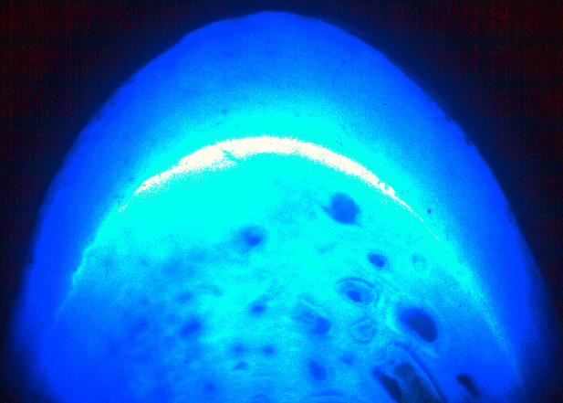
127

Figure 5. Overlaid magnified white light (visible)

(layer 1) and ultraviolet light image (layer 3) of a

loggerhead sea turtle humerus. The opacity of both image

layers was reduced to increase transparacy for aligning

physical markers and the edge of the bone. The opacity of the

growth ring traces (layer 2) was set to zero.

128

Figure 6. Magnified ultraviolet light image (layer 3) of a

loggerhead sea turtle humerus. Opacity of the magnified

white light (visible) and growth ring traces (layers 1 and 2)

were set to zero. The tetracycline mark was traced as a

separate overlaying layer (layer 4).

129

Figure 7. Growth and Tetracycline (layers 2 and 4) traces of

a magnified loggerhead sea turtle humerus. Opacity of the

magnified white light (visible) and ultraviolet light image

(layers 1 and 3) were set to zero. The number of growth

marks both distal and proximal to the tetracycline mark can

easily be counted.

130

Results

A tetracycline mark was easily identifiable on the

lateral edges of the bone (Figure 8). Dorsal and ventral

surfaces of the bone displayed highly compressed growth rings

and no evidence of a tetracycline mark, even under

magnification (Figure 2,4).

Identification of the growth rings surrounding the

tetracycline mark determined that externally there were seven

(dense) arrested growth rings; internally 2 rings were

identified (Figure 7). This indicates that there were eight

growing seasons, which correspond to the eight years between

the time the animal was marked and released and the time it

was recovered. The presence of a fluorescing growth mark,

8.3 years after the time of injection, and growth rings

prior to the mark, shows that tetracycline can be used in

long term growth studies in sea turtles and that growth rings

continue to be deposited on an annual basis.

131

Figure 8. Ultraviolet light lateral view of a loggerhead sea

turtle humerus. The tetracycline mark is easily identifiable

on the lateral edges of the bone. Dorsal and ventral

surfaces have compressed rings and are not visible.

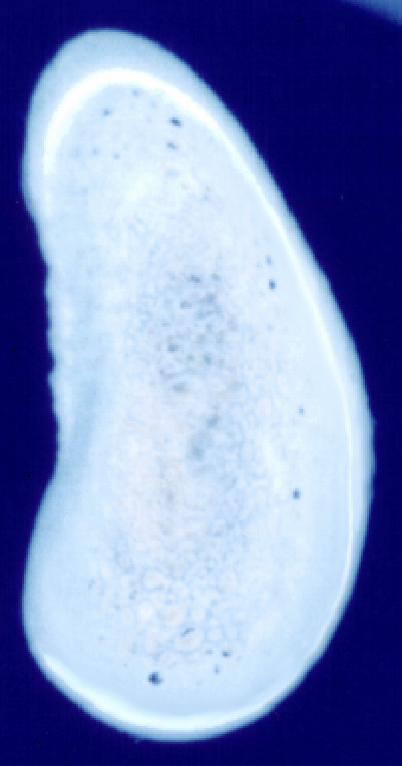
132

Discussion

Some studies indicated that tetracycline might not be

appropriate for long term studies because some recaptured

turtles showed no fluorescing ring (Klinger & Musick 1992),

or growth marks (Bjorndal et al. 1998). Many studies have

taken bone cores from the ventral surface of the humerus,

through the same region as our cross sections. These short

axis rings are compressed and often unreadable. The long

axis rings are more reliable and should be used for analysis

(Klinger 1988). Our study supports this opinion and suggests

that a better location to take bone cores is along the

sagittal axis of the bone.

One of the primary criteria for skeletochronology

studies is that physiologically important environmental

conditions (diet, food availability [feeding rates],

temperture, etc.) are not constant (Bjorndal et al. 1998, Zug

et al. 1986). It is the change in the conditions that cause

a corresponding change in growth rate, and rate of bone

deposition. It is important that validation studies not

violate the criteria for its use.

The Von Bertalanffy growth curve (Klinger 1988) roughly

fits the data recorded from this turtle (Figure 9, Table 1).

The age at first capture, calculated from the Von Bertalanffy

equation from a straight carapace length

133

Figure 9. A Von Bertalanffy growth curve (straight carapace

length) for loggerhead sea turtles, calculated by Klinger

(1988). Straight tip to tip measurements for the turtle are

plotted along the curve. For these comparisons the

measurements and corresponding age of first capture are

presumed correct. It is clear that the curve roughly fits

the data recorded from this turtle. The Von Bertalanffy

equation Lt = 111.9*(1-e(-0.076*(t+1.16))) calculates length from

age in years.

134

(SCL) of 91.2 cm, was 21.08 years old. The SCL at recapture

was 99.4 cm, for a growth rate of 0.99 cm/yr. This growth

rate is significantly lower than the range of 1.86-4.02 cm/yr

for turtles in the 90 cm class, and higher than the 1 meter

size class (0.64-0.67 cm/yr), discussed by Klinger (1988,

Klinger & Musick 1995) (Table 2). The turtles’ intermediate

growth rate suggests that it may have become sexually mature

and started nesting earlier than predicted by the age growth

curve. Miller (1997) cautions that size alone can not be

used to determine the maturity of the turtle. The allocation

of resources from growth to reproduction would account for

the differences (Hainsworth 1981).

Some sea turtle measurements increase in size over 25

times from hatchling to adult; the humerus, for example,

increases over tenfold in cross-section diameter (Zug et

al. 1986). This means there is extensive resorption and

deposition of the periosteal layers as the turtle grows

(Klinger 1988, Zug et al. 1986).

In conclusion, long term tetracycline studies of sea

turtles should not be dismissed. We have shown that clear,

distinctive growth marks can be identified after 8 years in

the wild, and growth marks continue to be deposited in

large mature sea turtles. Location of bone plug samples isa

critical part of the success of using tetracycline as a

skeletal marker. Bone plugs should be taken along the long

axis of the humerus. Additional studies to determine optimal

concentrations of oxytetracycline markers should continue.

135

This study clearly shows the viability of oxytetracycline use

as a skeletal marker for skeletochronology studies.

136

Table 1. Statistics and calculated values (age, straightcarapace length and growth rates) from the Von Bertalanffygrowth curve for loggerhead sea turtles, calculated byKlinger (1988). For these calculations the measurements andcorresponding age of first capture are presumed correct.(* indicates known values)

Date 20 Jun 1989 22 Sep 1997Time (yr) 8.255*Length (cm) 91.2* 99.4*Growth (cm) 8.2*Growth Rate (cm/yr) 0.99*Age from Curve (yr)based on Length

21.08 27.67

Predicted Length (cm)based on (Age1+Time)

100.88

Time (yr) based onGrowth and Age1

6.59

137

Table 2. Growth rate(s) from our tetracycline recapture andcalculated mean growth rates, standard deviation and rangefor two size classes of loggerhead sea turtles, from Klinger(1988).

Size (class) SampleSize

Mean GrowthRate(cm/yr)

StandardDeviation

Range

90.0-99.9 7 2.87 0.85 1.86-4.02

Recapture 1 0.99 0.99

100.0-110.0 2 0.66 0.02 0.64-0.67

138

Literature Cited

Bjorndal, K.A., A.B. Bolten, R.A.Bennett, E.R. Jacobson, T.J.

Wronski, J.J. Valeski, & P.J. Eliazar. 1988. Age and

Growth in Sea Turtles: Limitations of Skeletochronology for

Demographic Studies. Copeia (1):23-30.

Chaloupka, M.Y. & J.A. Musick. 1997. Age, Growth and

Population Dynamics. IN: P.L. Lutz and J.A. Musick (eds.).

The Biology of Sea Turtles. CRC Press. New York, NY, USA.

pp. 233-276.

Frost, H.M., A.R. Villanueva, H. Roth & S. Stanisavijevic.

1961. Tetracycline Bone Labeling. J. New Drugs. 1(5):206-

216.

Hainsworth, F.R. 1981. Animal Physiology Adaptations in

Functions. Addison-Wesley Publishing Company, Inc.,

Reading MA. pp. 669.

Harris, W.H. 1960. A Microscopic Method of Determining

Rates of Bone Growth. Nature. 188(4755):1038-1039.

Klinger, R.C., 1988. Age and Growth of Juvenile Loggerheads,

(Caretta caretta), from Chesapeake Bay. Unpublished

Master's Thesis. School of Marine Science, VIMS, College of

William and Mary, Gloucester Pt., VA. pp.89.

Klinger, R.C., R.H. George, J.A. Musick, 1997. A Bone Biopsy

Technique for Determining Age and Growth in Sea Turtles.

Herpetological Review. 28(1):31-32p.

Klinger, R.C., J.A. Musick, 1995. Age and Growth of

Loggerhead Turtles (Caretta caretta) from Chesapeake Bay.

Copeia 1995(1):204-209.

139

Klinger, R.C., J.A. Musick, 1992. Annular Growth Layers in

Juvenile Loggerhead Sea Turtles (Caretta caretta).

Bulletin of Marine Science 51(2):224-230.

Meylan, A.B., 1982. Sea turtles migration-evidence from tag

returns. In K. Bjorndal (ed.), Biology and conservation of

sea turtles. Smithsonian Institution Press, Washington,

D.C. pp.91-100.

Zug, G.R., A.H. Wynn, and C. Ruckdeschel. 1986. Age

determination of loggerhead sea turtles, Caretta caretta,

by incremental growth marks in the skeleton. Smithsonian

Contributions to Zoology. #427. pp. 34.

140

Aspects of the Biology of Sea Turtles in the

Mid-Atlantic Bight.

141

CONCLUSION

The objectives of this dissertation were to compile,

review and analyze several different aspects of the biology

of sea turtles that utilize the Chesapeake Bay as a seasonal

foraging habitat. Many of these results substantiate,

collaborate and refine previous research. I summarize the

results from each study here:

Several trends in turtle stranding data were

established. There were gross increases in numbers of

stranded turtles for loggerheads (3 turtles/year), Kemp’s

ridleys (0.7 turtles/year) and leatherbacks (0.5

turtles/year). The cause of death for most (84%) of these

turtles was either undetermined or unrecorded. Of the

turtles with recorded causes of death the most significant

interaction appeared to be with boats. Understandably this

cause of turtle mortality is very hard to monitor and

quantify. Over half of the turtle deaths each year occur in

the spring when turtles migrate into the Bay (Kemp’s ridleys

have a second significant stranding peak during the fall

migration). The number of possible anthropomorphic

interactions with turtles has increased as recreational

boating & fishing has increased in popularity. Future cause

of mortality data may be enhanced by increasing volunteer

training and network diligence.

The turtles that strand in the Bay are primarily

juveniles of each species; reproductive adults rarely strand.

Among loggerheads, stranded turtles’ appear to be normally

142

distributed, in terms of size, whereas the Kemp’s ridleys

have an erratic pattern. The difference may be explained by

yearly hatchling success of the ridleys because of their

panmictic evolution. Loggerheads are much less susceptible

to localized stresses (beach erosion, storms, human and

animal interactions) because they nest throughout the

southern coastal United States.

During migration periods, sea turtle strandings occur

most commonly on the Southern Bay and Virginia Beach, Ocean

regions; at other times strandings are spread throughout the

Bay. The spatial trends probably do not represent true

stranding patterns for several reasons. First the beaches

are not uniformly sampled. Many beaches are inaccessible,

even by boat, because of marsh boundaries, bars and islands.

Other beaches (Southern Bay and Virginia Beach areas) are

wide sandy beaches that are used daily by thousands of people

and so are extensively monitored.

Sea turtle morphology data from the VIMS data set

provides a solid base for future studies. Regressions

calculated from the morphology data often explain more than

90% of the variation in the measurements. The remaining 10%

of variance can easily be explained by such factors as: (1)

poor condition of the turtle when measured; (2) inexperience

of measurers and procedural variations (hundreds of

volunteers made measurements); (3) location and accessibility

of animal when measured. There were no morphologic

differences identified between the two genetic populations of

143

juvenile loggerheads found in the Bay. The regression

equations can serve as excellent estimators for missing and

suspect data. Many missing values are required for State and

Federal management agencies and future research.

The carapace morphology of loggerheads and Kemp’s

ridleys changes as the turtles grow. The carapace flattens

out in larger individuals, presumably to maintain a

relatively constant amount of lift while swimming. The

velocity of hatchling turtles is much less than the adults

(Wyneken 1997). To maintain the same lift the carapace would

need to have a higher dome. The larger (faster) turtles are

flatter, and so maintain a relative (constant) amount of

lift. Extra lift may be needed in hatchlings because of

their swimming inefficiency; their Reynolds numbers (1.2E4 to

3E5) are much lower than other aquatic migrants (Wyneken

1997, Vogel 1981). This might also explain the domed shape

of the hatchling carapace.

The Magnetic Resonance Imaging (MRI) techniques

developed by Coles (1994) were used to image juvenile Kemp’s

ridley and loggerhead sea turtle heads. The location of

magnetic particles in the sea turtle heads appears in the

same region as birds and fish. The anomalies appeared to be

paired (left and right). This bilateral symmetry suggests a

possible use as a sensory system. This suggests that the MRI

can be used for determining positions of electromagnetic

stimulus in neurological studies. Unfortunately we have also

verified the sensitivity of the MRI to magnetic

144

contamination. Future studies must take extra precautions

against contamination.

There have been no studies on the natural preferred

behavioral temperature preferences of marine turtles. Using

satellite imaging technology we were able to confirm the

temperature limits determined by others (Epperly et al. 1995,

Schwartz 1978, Faulkner & Binger 1927). The turtles observed

were within a range of 13oC to 29oC, well within the

previously established physiological limits and the entrance

and exit temperatures of turtles during migration into and

out of the Bay.

There have been many studies of age and growth in

ectothermic vertebrates using oxytetracycline as a

skeletochronological marker (Zug et al. 1986), but these

studies have usually been of short (1-2 year) duration. As a

result, questions have been raised as to whether

oxytetracycline will stay in the bone matrix for longer

periods and whether growth marks are deposited annually in

older turtles (Bjorndal et al. 1998, Klinger & Musick 1992).

The results from a turtle injected with oxytetracycline eight

years before recapture suggest otherwise. Sampling whole

cross sections of the humerous suggest that the area

frequently used for taking bone cores (used in previous

studies) is inappropriate, and that the lateral edges of the

humerous, or perhaps other bones, should be used for long

term studies. The growth rates and ring deposition support

Klinger’s (1988) data, although it suggests that sexual

145

maturity may be occurring at an earlier age (smaller size)

than previously believed.

There is a need for long term continuous monitoring of

populations of threatened and endangered species,

particularly in areas that concentrate animals such as;

nesting beaches, juvenile nursery habitats. For example, for

three weeks in the spring of 1998 a major stranding event,

possibly precipitated by a spring fishery near the mouth of

the Bay, went unnoticed (Coles & Musick 1998). By the time

fishery managers (NMFS, VMRC) discovered what was happening

the cause of the event had disappeared. During this period

100’s of loggerheads and Kemp’s ridleys had stranded. The

lapse in monitoring is a conservation catastrophe and

emphasizes the need for continuous data collection and

monitoring. It is also important for these monitoring

databases to have good and consistent data management.

Fisheries and resource managers should recognize these issues

and take steps to alleviate the problems, by providing

adequate resources to manage and maintain these types of

valuable monitoring data.

146

Literature Cited

Bjorndal, K.A., A.B. Bolten, R.A. Bennett, E.R. Jacobson,

T.J.Wronshi, J.J. Valeshi, and P.J. Eliazar. 1998. Age and

growth in sea turtles: Limitations of skeletochronology for

demographic studies. Copeia. 1:23-30.

Coles, W.C. 1994. Localization of magnetic particles in animal


State University of New York, Geneseo. pp. 39.

Coles, W.C. an J.A. Musick. 1998. Record numbers of sea turtle

strandings in Virginia in May and June 1998. Virginia

Institute of Marine Science, Gloucester Pt., VA, Marine

Resource Report Number 98-4. pp.8.

Epperly, S.P., J. Braun, A.J. Chester, F.A. Cross, J.V.

Merriner, and P.A. Tester. 1995. The winter distribution of

sea turtles in the vicinity of Cape Hatteras and their

interactions with the summer flounder trawl fishery. Bull.

Mar. Sci. 56:547-568.

Faulkner, J.M. and C.A.L. Binger 1927. Oxygen poisoning in cold

blooded animals. J. Exp. Med. 45(5):865-871.

Klinger, R.C., 1988. Age and Growth of Juvenile Loggerheads,

(Caretta caretta), from Chesapeake Bay. Unpublished Master's

Thesis. School of Marine Science, VIMS, College of William

and Mary, Gloucester Pt., VA pp. 89.

Klinger, R.C., J.A. Musick, 1992. Annular Growth Layers in

Juvenile Loggerhead Sea Turtles (Caretta caretta). Bulletin

of Marine Science 51(2):224-230.

147

Schwartz, F.J. 1978. Behavioral and tolerance responses to cold

water temperatures by three species of sea turtles (Reptilia,

Chelonidae) in North America. p.16-18. In: G.E.Henderson

(ed). Proceedings of the Florida and Interregional

Conference on Sea Turtles, 24-25 July 1976, Jensen Beach

Florida.

Vogel, S. 1981. Life in Moving Fluids. Princeton University

Press, Princeton, NJ. pp. 352.

Wyneken, J. 1997. Sea Turtle Locomotion: Mechanisms, Behavior

and Energetics. IN Lutz, P.L. and J.A. Musick, 1997. The

Biology of Sea Turtles. CRC Press. New York, NY, USA. 165-

198 pp.

Zug, G.R., A.H. Wynn, and C. Ruckdeschel. 1986. Age

determination of loggerhead sea turtles, Caretta caretta, by

incremental growth marks in the skeleton. Smithsonian

Contributions to Zoology. #427 pp. 34.

148

Appendix 1. Recipes

Roix Sea Turtle Deluxe.

2 Onions salt brown flourParsley pepper butterThyme cloves Allspiceglass of Claret or Madeira Wine 1 Sea Turtle

Kill the turtle at Daylight in the Summer (the nightbefore in the Winter), and hang it up to bleed. Afterbreakfast, scald it well and scrape the outer skin off theshell. Open it carefully, so as not to break the Gall.Break both shells to pieces and put them into the pot. Laythe fins, the eggs and some of the more delicate parts by.Put the rest into the pot with a quantity of water to suitthe size of your family. Add 2 onions, parsley, thyme, salt,pepper, cloves, and allspice to suit your taste.

Simmer turtle fins in boiling water until tender andthen skinned. Dip the fins in brown flour and fry them inbutter. When they are nicely browned, add a little whitewine. Simmer until tender.

About half an hour before dinner thicken the soup withbrown flour and butter rubbed together. An hour beforedinner, take the parts laid by, roll them in brown flour, frythem in butter, put them and the eggs in the soup; justbefore dinner add a glass of Claret or Madeira Wine.

Adapted from: A Herpetological Cookbook. Ed. Ernest A. Liner, 310Malibou Blvd. Houma, Louisiana 70360, and The Williamsburg art ofcookery, or Accomplished gentle-womans companion: Being a collection ofupwards of 500 of the most ancient and approved recipes of Virginiacookery. Ed. Helen Bullock, Deets Press, Richmond, VA.

149

St. cRoix Turtle Extravaganza.

Sea Turtle meat Can Ro-Tel tomatoes4 hardboiled eggs 2 minced bell peppers1/2 cup flour 4 large minced onions1/2 cup oil Can tomatoes #26 cloves garlic Thyme4 stalks minced celery Sweet basil1/4 cup Parsley waterCayenne 3/4 cup scallion tops

Season turtle meat with salt and cayenne, brown thoroughly inhot oil. Remove meat and add the onions, stirring until deepbrown and all pan drippings are absorbed. Add the tomatoesand cook down until browned, also. Add bell pepper, celery,garlic, thyme, sweet basil and water. Let simmer about 1hour until vegetables are done. Add turtle meat and boiledeggs and cook slowly until turtle is done, about 2 hours.Add sherry, parsley and scallions last 5 minutes. Serve overrice.

Modified from: A Herpetological Cookbook. Ed. Ernest A. Liner, 310Malibou Blvd. Houma, Louisiana 70360.

aspects of the biology of sea turtles in … table of contents approval ii dedication iii table of...

Documents