asian economic and social society - government bond market integration in asean3)-289-312.pdf ·...

289

© 2020 AESS Publications. All Rights Reserved.

GOVERNMENT BOND MARKET INTEGRATION IN ASEAN COUNTRIES

Masao Kumamoto1+

Juanjuan Zhuo2

1Graduate School of Business Administration, Hitotsubashi University, Tokyo, Japan.

2Faculty of Humanities and Social Sciences, Kochi University, Kochi, Japan.

(+ Corresponding author)

ABSTRACT Article History Received: 25 November 2019 Revised: 9 January 2020 Accepted: 12 February 2020 Published: 24 March 2020

Keywords Government bond market integration ASEAN Dynamic factor model Dynamic conditional correlation (DCC) Pooled mean estimation (PMG)

Threshold analysis.

JEL Classification: E43; G12; G15.

The development and the integration of the bond market is becoming an important policy issue in ASEAN countries. We investigate government bond market integration in four ASEAN countries. We first decompose yields in ASEAN countries and the United States into global and regional factors using the approximate dynamic factor model. Next, we employ the dynamic conditional correlation method to find that regional markets have been integrated in the sense that their yields are highly and positively correlated with the common regional factor. We also find that the correlation between the global factor and the yield has different signs in different countries. Therefore, we use the pooled mean estimation method to investigate the determinants that make the correlation positive in some countries and negative in others. We find that public interest payments is an important determinant and discover a threshold that depends on public interest payments. The global factor has a significantly negative effect on the yield spread when public interest payments are above the threshold value. From above results, we can conclude that market discipline has been operating in the four ASEAN government bond markets in the sense that investors discriminate between the creditworthiness of the governments’ bonds by focusing on the public interest payments.

Contribution/ Originality: This study is one of very few studies which have investigated the government bond

market integration by considering the correlation between the yield in each country and the regional or the global

factor. We also investigate the determinants of the correlation between the yield and the global factor.

1. INTRODUCTION

Regional economic integration among Association of South East Asian Nations (ASEAN) countries has

progressed steadily on the real economic side. Since the ASEAN Free Trade Area (AFTA) was signed in 1992, a

Common Effective Preferential Tariff (CEPT) Scheme and its successor, the ASEAN Trade in Goods Agreement

(ATIGA), have played a main role in intra-ASEAN free trade in goods. In addition to trade in goods, the 1995

ASEAN Framework Agreement on Services (AFAS) liberalized intra-ASEAN trade in services, and the 1998

ASEAN Investment Area (AIA) created a liberal, transparent environment for investment in the ASEAN region.

The establishment of the ASEAN Economic Community (AEC) in 2015 is a symbolic milestone in ASEAN regional

economic integration on the real economic side.

Asian Economic and Financial Review ISSN(e): 2222-6737 ISSN(p): 2305-2147 DOI: 10.18488/journal.aefr.2020.103.289.312 Vol. 10, No. 3, 289-312. © 2020 AESS Publications. All Rights Reserved. URL: www.aessweb.com

http://crossmark.crossref.org/dialog/?doi=10.18488/journal.aefr.2020.103.289.312&domain=pdf&date_stamp=2017-01-14

https://orcid.org/0000-0003-2839-7874

https://orcid.org/0000-0002-5287-6368

http://www.aessweb.com/

http://www.aessweb.com/journals/March2020/5002/4906

Asian Economic and Financial Review, 2020, 10(3): 289-312

290


Unlike on the real economic side, however, the ASEAN economy is still fragile on the financial side. The

―double mismatch in currency and maturity‖ in financing are recognized has having been among the main causes of

the 1997 Asian currency crisis. ASEAN countries depended on short-term foreign currency-denominated bank

loans from foreign banks to finance longer-term domestic investment. ASEAN countries have accumulated

domestic savings since the crisis. However, much of those savings flowed overseas, especially to the United States,

before flowing back into Asian countries. As a result, ASEAN countries have accumulated huge foreign reserves, a

large portion of which is in the form of US Treasury securities, while receiving foreign direct and portfolio

investments to finance domestic firms. This means that ASEAN’s large intraregional savings have not been utilized

to finance intraregional investment.

Therefore, the development of the financial intermediary function, especially regional bond markets, is

becoming an important policy issue in Asia. It is necessary to reform and harmonize regulations in accordance with

international standards and then facilitate regional bond market integration. Accordingly, the Asian Bond Markets

Initiative (ABMI) was launched by the ASEAN+3 Finance Ministers’ and Central Bank Governors’ Meeting in

August 2003. The Executives’ Meetings of East Asia and Pacific Central Banks (EMEAP) also launched the Asian

Bond Fund (ABF) in June 2003. Through these domestic and regional efforts, Asian bond markets have grown

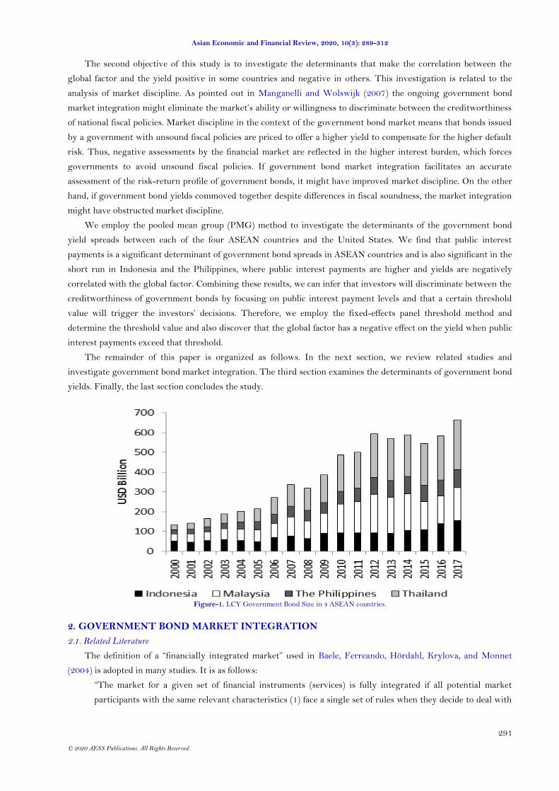
rapidly and are considered to be undergoing regional integration. Figure 1 shows the amount of outstanding local

currency-denominated government bonds in four ASEAN countries: Indonesia, Malaysia, the Philippines, and

Thailand. We can see that the government bond markets in the region have grown rapidly, from about 130 billion

US dollars in 2000 to about 570 billion US dollars in 2017.

Bond market integration among Asian countries facilitates greater capital mobility, which can improve the

efficiency of capital allocation and hence enhance financial development and economic growth in the region. It also

enables investors to diversify their portfolios at a low cost, which can eliminate country-specific risks.

The first objective of this study is to investigate whether the government bond markets are integrated in the

four ASEAN countries listed above: Indonesia, Malaysia, the Philippines, and Thailand. We investigate only four

countries due to data availability issues. We focus on government bond market integration because integration is a

pre-requisite for the development of regional bond markets, including corporate bond markets. Government bond

markets provide a risk-free benchmark yield curve for corporate bonds and also support the derivatives market.

As the first step in our analysis, we will employ an approximate dynamic factor model to decompose yields in

the four ASEAN countries and the United States into three factors. The first is a global factor that is highly and

positively related to the yield in the United States but also affects the yields in ASEAN countries. The second is a

regional factor that affects the yields in ASEAN countries highly and positively but is not explained by the global

factor. The last is an idiosyncratic shock, based on the idea that idiosyncratic shock can be diversified away via

international investment in the integrated market, so that the yield should be influenced only by common factors.

This means that, if the government bond market in one country is integrated with the regional (global) government

bond market, then the yield in this country might be correlated positively and highly with the regional (global)

factor. Therefore, in the second step, we will employ a dynamic conditional correlation (DCC) model to calculate the

time-varying conditional correlation between each factor and the yield in each country. The results show that the

correlations between the regional factor and the yield in each ASEAN country are significantly positive and high,

implying that government bond yields in ASEAN countries are driven by the common regional factor and thus that

regional government bond markets are integrated. On the other hand, the correlations between the global factor

and the yield in each country have different signs, showing a positive correlation in Malaysia and Thailand and a

negative correlation in Indonesia and the Philippines. This means that the effects of the global factor across

countries are asymmetric. This leads to a question: Why are the effects of the global factor asymmetric among the

four ASEAN countries, and which variables indicate the creditworthiness of government bonds?


291


The second objective of this study is to investigate the determinants that make the correlation between the

global factor and the yield positive in some countries and negative in others. This investigation is related to the

analysis of market discipline. As pointed out in Manganelli and Wolswijk (2007) the ongoing government bond

market integration might eliminate the market’s ability or willingness to discriminate between the creditworthiness

of national fiscal policies. Market discipline in the context of the government bond market means that bonds issued

by a government with unsound fiscal policies are priced to offer a higher yield to compensate for the higher default

risk. Thus, negative assessments by the financial market are reflected in the higher interest burden, which forces

governments to avoid unsound fiscal policies. If government bond market integration facilitates an accurate

assessment of the risk-return profile of government bonds, it might have improved market discipline. On the other

hand, if government bond yields commoved together despite differences in fiscal soundness, the market integration

might have obstructed market discipline.

We employ the pooled mean group (PMG) method to investigate the determinants of the government bond

yield spreads between each of the four ASEAN countries and the United States. We find that public interest

payments is a significant determinant of government bond spreads in ASEAN countries and is also significant in the

short run in Indonesia and the Philippines, where public interest payments are higher and yields are negatively

correlated with the global factor. Combining these results, we can infer that investors will discriminate between the

creditworthiness of government bonds by focusing on public interest payment levels and that a certain threshold

value will trigger the investors’ decisions. Therefore, we employ the fixed-effects panel threshold method and

determine the threshold value and also discover that the global factor has a negative effect on the yield when public

interest payments exceed that threshold.

The remainder of this paper is organized as follows. In the next section, we review related studies and

investigate government bond market integration. The third section examines the determinants of government bond

yields. Finally, the last section concludes the study.

Figure-1. LCY Government Bond Size in 4 ASEAN countries.

2. GOVERNMENT BOND MARKET INTEGRATION

2.1. Related Literature

The definition of a ―financially integrated market‖ used in Baele, Ferreando, Hördahl, Krylova, and Monnet

(2004) is adopted in many studies. It is as follows:

―The market for a given set of financial instruments (services) is fully integrated if all potential market

participants with the same relevant characteristics (1) face a single set of rules when they decide to deal with


292


those financial instruments (services); (2) have equal access to the above-mentioned set of financial

instruments and/or services; (3) are treated equally when they are active in the market.‖

The direct implication of this definition of financial integration is that assets with the same risk level should

have the same expected returns; thus, the law of one price must hold because all agents will be free to exploit any

arbitrage opportunities. The indicator considered as evidence of the law of one price varies depending on the focus

of the study. Some studies focus on price convergence, while others focus on sensitivity, mutual causality,

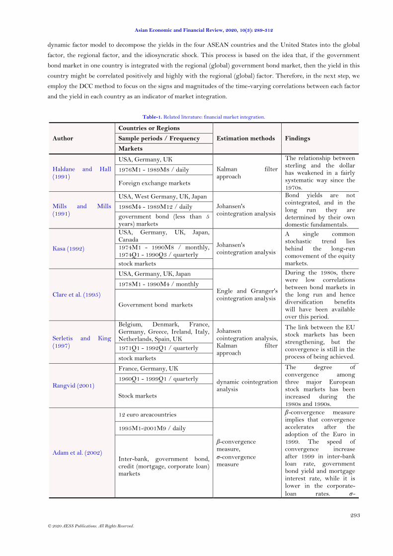
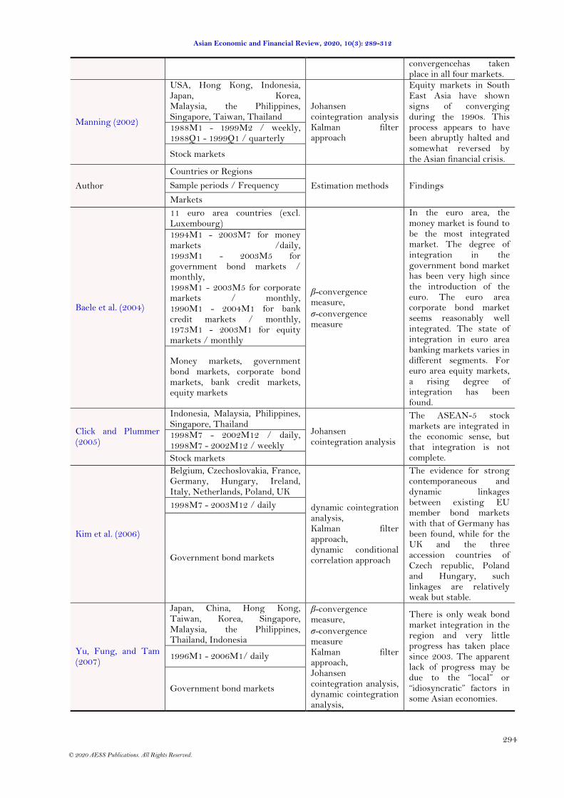
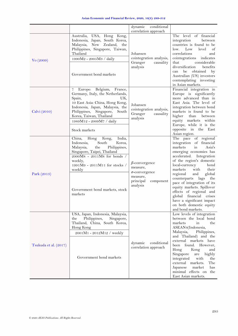
cointegration relationship, market cycle synchronization, and correlation. Table 1 summarizes the approaches to

estimation methods in the related literature.

Adam, Jappeli, Menichini, Padula, and Pagano (2002); Baele et al. (2004) and Park (2013) employed -

convergence and -convergence measures, which are borrowed from the economic growth literature. -

convergence is based on the idea that higher yields tend to decrease more rapidly, and it examines convergence

speed. On the other hand, -convergence examines the cross-sectional dispersion in yields to measure the financial

integration level at any point in time.

Serletis and King (1997) and Kim, Lucey, and Wu (2006) employed Haldane and Hall (1991) approach. This is

based on the Kalman filter method and regresses the yield spread between one country and the internal regional

benchmark country (, ,i t rb ti i ) against the yield spread between the internal benchmark country and the external

global benchmark country (, ,rb t gb ti i )1 . If convergence with the internal (external) benchmark country has

occurred, the time-varying coefficient will converge toward zero (one) over time.

Mills and Mills (1991); Kasa (1992); Clare, Maras, and Thomas (1995); Serletis and King (1997); Manning

(2002); Click and Plummer (2005); Vo (2009) and Calvi (2010) employed the cointegration method. Yields in

integrated financial markets cannot diverge arbitrarily from each other; therefore, there must be a stable long-run

relationship among yields across countries. Moreover, the number of common stochastic trends will equal the

dimension of the system (n) minus the number of linear independent cointegrating vectors—namely, the

cointegration rank (r). Therefore, if the cointegration rank is n-1, there is a single common stochastic trend, which

provides evidence of a fully integrated financial market. This means that the yields in the process of integration are

expected to increase the number of cointegrations. Based on this idea, Rangvid (2001) and Kim et al. (2006)

employed the dynamic cointegration method to detect the time-varying number of cointegration ranks by rolling

the estimation window.

Kim et al. (2006) and Tsukuda, Shimada, and Miyakoshi (2017) employed the DCC method proposed by Engle

(2002). This method is based on the idea that higher correlation between markets indicates greater return

comovement and thus greater market integration.

We will develop the DCC method by employing the approximate dynamic factor model proposed by Stock and

Mark (1998); Stock and Mark (2002a); Stock. and Mark (2002b). The - and -convergence measures and Haldane

and Hall (1991) approach cannot be applied directly to our study since the regional and global benchmark countries

to which the yields in the four ASEAN countries converge cannot be chosen a priori and arbitrarily.2 In addition,

the cointegration method is limited in the sense that the existence of a cointegration relationship does not

necessarily imply that their yields comove. For example, if the yields in two countries are perfectly negatively

correlated, the cointegration vector [1, -1] might be detected. Instead, we will first employ the approximate

1 For example, Germany can be regarded as an internal regional benchmark country, while the United States can be regarded as an external global benchmark

country for euro nations.

2 This problem holds for the DCC method. For example, Kim et al. (2006) used the DCC method to investigate government bond market integration in EU countries.

For such countries, Germany seems to be the preferred benchmark country.


293


dynamic factor model to decompose the yields in the four ASEAN countries and the United States into the global

factor, the regional factor, and the idiosyncratic shock. This process is based on the idea that, if the government

bond market in one country is integrated with the regional (global) government bond market, then the yield in this

country might be correlated positively and highly with the regional (global) factor. Therefore, in the next step, we

employ the DCC method to focus on the signs and magnitudes of the time-varying correlations between each factor

and the yield in each country as an indicator of market integration.

Table-1. Related literature: financial market integration.

Author

Countries or Regions

Estimation methods Findings Sample periods / Frequency

Markets

Haldane and Hall (1991)

USA, Germany, UK

Kalman filter approach

The relationship between sterling and the dollar has weakened in a fairly systematic way since the 1970s.

1976M1 - 1989M8 / daily

Foreign exchange markets

Mills and Mills (1991)

USA, West Germany, UK, Japan

Johansen's cointegration analysis

Bond yields are not cointegrated, and in the long run they are determined by their own domestic fundamentals.

1986M4 - 1989M12 / daily

government bond (less than 5 years) markets

Kasa (1992)

USA, Germany, UK, Japan, Canada

Johansen's cointegration analysis

A single common stochastic trend lies behind the long-run comovement of the equity markets.

1974M1 - 1990M8 / monthly, 1974Q1 - 1990Q3 / quarterly

stock markets

Clare et al. (1995)

USA, Germany, UK, Japan

Engle and Granger's cointegration analysis

During the 1980s, there were low correlations between bond markets in the long run and hence diversification benefits will have been available over this period.

1978M1 - 1990M4 / monthly

Government bond markets

Serletis and King (1997)

Belgium, Denmark, France, Germany, Greece, Ireland, Italy, Netherlands, Spain, UK

Johansen cointegration analysis, Kalman filter approach

The link between the EU stock markets has been strengthening, but the convergence is still in the process of being achieved.

1971Q1 - 1992Q1 / quarterly

stock markets

Rangvid (2001)

France, Germany, UK

dynamic cointegration analysis

The degree of convergence among three major European stock markets has been increased during the 1980s and 1990s.

1960Q1 - 1999Q1 / quarterly

Stock markets

Adam et al. (2002)

12 euro areacountries

β-convergence measure,

σ-convergence measure

β-convergence measure implies that convergence accelerates after the adoption of the Euro in 1999. The speed of convergence increase after 1999 in inter-bank loan rate, government bond yield and mortgage interest rate, while it is lower in the corporate-

loan rates. σ-

1995M1-2001M9 / daily

Inter-bank, government bond, credit (mortgage, corporate loan) markets


294


convergencehas taken place in all four markets.

Manning (2002)

USA, Hong Kong, Indonesia, Japan, Korea, Malaysia, the Philippines, Singapore, Taiwan, Thailand

Johansen cointegration analysis Kalman filter approach

Equity markets in South East Asia have shown signs of converging during the 1990s. This process appears to have been abruptly halted and somewhat reversed by the Asian financial crisis.

1988M1 - 1999M2 / weekly, 1988Q1 - 1999Q1 / quarterly

Stock markets

Author

Countries or Regions

Estimation methods Findings Sample periods / Frequency

Markets

Baele et al. (2004)

11 euro area countries (excl. Luxembourg)


σ-convergence measure

In the euro area, the money market is found to be the most integrated market. The degree of integration in the government bond market has been very high since the introduction of the euro. The euro area corporate bond market seems reasonably well integrated. The state of integration in euro area banking markets varies in different segments. For euro area equity markets, a rising degree of integration has been found.

1994M1 - 2003M7 for money markets /daily, 1993M1 - 2003M5 for government bond markets / monthly, 1998M1 - 2003M5 for corporate markets / monthly, 1990M1 - 2004M1 for bank credit markets / monthly, 1973M1 - 2003M1 for equity markets / monthly

Money markets, government bond markets, corporate bond markets, bank credit markets, equity markets

Click and Plummer (2005)

Indonesia, Malaysia, Philippines, Singapore, Thailand

Johansen cointegration analysis

The ASEAN-5 stock markets are integrated in the economic sense, but that integration is not complete.

1998M7 - 2002M12 / daily, 1998M7 - 2002M12 / weekly

Stock markets

Kim et al. (2006)

Belgium, Czechoslovakia, France, Germany, Hungary, Ireland, Italy, Netherlands, Poland, UK

dynamic cointegration analysis, Kalman filter approach, dynamic conditional correlation approach

The evidence for strong contemporaneous and dynamic linkages between existing EU member bond markets with that of Germany has been found, while for the UK and the three accession countries of Czech republic, Poland and Hungary, such linkages are relatively weak but stable.

1998M7 - 2003M12 / daily


Yu, Fung, and Tam (2007)

Japan, China, Hong Kong, Taiwan, Korea, Singapore, Malaysia, the Philippines, Thailand, Indonesia


σ-convergence measure Kalman filter approach, Johansen cointegration analysis, dynamic cointegration analysis,

There is only weak bond market integration in the region and very little progress has taken place since 2003. The apparent lack of progress may be due to the ―local‖ or ―idiosyncratic‖ factors in some Asian economies.

1996M1 - 2006M1/ daily



295


dynamic conditional correlation approach

Vo (2009)

Australia, USA, Hong Kong, Indonesia, Japan, South Korea, Malaysia, New Zealand, the Philippines, Singapore, Taiwan, Thailand Johansen

cointegration analysis, Granger causality analysis

The level of financial integration between countries is found to be low. Low level of correlations and cointegrations indicates that considerable diversification benefits can be obtained by Australian (US) investors contemplating investing in Asian markets.

1990M2 - 2005M3 / daily


Calvi (2010)

7 Europe: Belgium, France, Germany, Italy, the Netherlands, Spain, UK, 10 East Asia: China, Hong Kong, Indonesia, Japan, Malaysia, the Philippines, Singapore, South Korea, Taiwan, Thailand

Johansen cointegration analysis, Granger causality analysis

Financial integration in Europe is significantly more advanced than in East Asia. The level of integration between bond markets is found to be higher than between equity markets within Europe, while it is the opposite in the East Asian region.

1989M12 - 2009M7 / daily

Stock markets

Park (2013)

China, Hong Kong, India, Indonesia, South Korea, Malaysia, the Philippines, Singapore, Taipei, Thailand


σ-convergence measure, principal component analysis

The pace of regional integration of financial markets in Asia's emerging economies has accelerated. Integration of the region's domestic local-currency bond markets with their regional and global counterparts lags the pace of integration of its equity markets. Spillover effects of regional and global financial crises have a significant impact on both domestic equity and bond markets.

2000M8 - 2011M8 for bonds / weekly, 1991M9 - 2011M11 for stocks / weekly

Government bond markets, stock markets

Tsukuda et al. (2017)

USA, Japan, Indonesia, Malaysia, the Philippines, Singapore, Thailand, China, South Korea, Hong Kong

dynamic conditional correlation approach

Low levels of integration between the local bond markets in the ASEAN4(Indonesia, Malaysia, Philippines, and Thailand) and the external markets have been found. However, Hong Kong and Singapore are highly integrated with the external markets. The Japanese market has minimal effects on the East Asian markets.

2001M1 - 2012M12 / weekly



296


2.2. Methodology

Let , , , , , ,[ , , , ]t id t my t ph t th t us tX i i i i i be a 5 1 vector composed of the standardized government bond yields in

Indonesia, Malaysia, the Philippines, Thailand, and the United States. Using an approximate dynamic factor model,

we decompose the vector as:

g g g g g gid my ph th us t

t t t tr r r r g rid my ph th us t

fX f

f

, (1)

where g

tf is the global factor, which is highly and positively related to the yield in the United States but also

affects the yields in ASEAN countries. r

tf is a regional factor, which is highly and positively related to the yields in

ASEAN countries but is not explained by the global factor. t is a 5 1 vector of idiosyncratic shock, and is a

5 2 factor loading matrix.

Next, we assume that the 3 1 vector ,[ ]g r

t i t t tY i f f follows the VAR(p) model,

0

1

p

t i t i t

i

Y A AY

,

1

2t t tH , 1 (0, )t t tI N H , (2)

where tH is a 3 3 conditional covariance matrix, and

t is an 3 1 innovation vector following an i.i.d.

standard normal distribution.

We can decompose the conditional covariance matrix tH as

1 1

2 2t t t tH D R D , (3)

where tD is a 3 3 diagonal matrix of time-varying standard deviations with

,ii th ( 1, ,3i ) as the ith

element of the diagonal，and tR is a 3 3 symmetric time-varying correlation matrix,

11,

22,

33,

0 0

0 0

0 0

t

t t

t

h

D h

h

,

12, 11, 22, 13, 11, 33,

12, 11, 22, 23, 22, 33,

13, 11, 33, 23, 22, 33,

1 / /

/ 1 /

/ / 1

t t t t t t

t t t t t t t

t t t t t t

h h h h h h

R h h h h h h

h h h h h h

.

The DCC model is estimated through a two-step procedure. In the first step, we obtain tD by assuming that

,ii th follows a GARCH (1, 1) process:

2

, 1 , 1 1 , 1ii t i i i t i ii th h . (4)

The specification of Equation 4 can be justified by the well-known results that GARCH(1,1) model can provide

a better fit and exhibit a more reasonable lag structure than the other specification.


297


In the second step, we standardize the residuals as

1

2t t tD

, namely as , ,i t it ii th , and use them to

estimate dynamic correlation. From Equation 3 we can see that

1 1

2 21 ( ) ( )t t t t t t tE D H D R

. (5)

The correlation matrix tR in Equation 5 can be estimated by specifying matrix tQ as the following

exponential smoother equation:

1 2 1 1 1 2 1(1 )t t t tQ R Q

. (6)

tQ is a 3 3 symmetric positive definite matrix, [ ]t tR E is the unconditional covariance matrix of the

standardized residuals (unconditional correlation), and 1

2 are non-negative parameters that satisfy

1 20 1 . Note that Equation 6 is used solely to provide tR.

The conditional correlation matrix tR is

obtained by

1 1

2 2( ) ( )t t t tR diag Q Q diag Q

, (7)

where 1/ 2( )tdiag Q is a diagonal matrix of the square root of the diagonal element of tQ . For

tR in Equation

7 to be positive definite, the only condition that needs to be satisfied is that tQ is positive definite.

2.3. Empirical results

2.3.1. Data

Our sample comprises Indonesia, Malaysia, the Philippines, and Thailand. As mentioned, we exclude the other

ASEAN countries (including Singapore) from our sample due to data availability issues.

Our sample period runs from January 2, 2001 to June 30, 2018, and we use daily data. We calculate the

government bond yields from the 10-year government bond total index data denominated in local currency (LCY).

The data for ASEAN countries are sourced from AsiaBondsOnline, and the US data come from Datastream.

2.3.2. Empirical Results

As the first step, we decompose the yields in ASEAN countries and the United States into the global factor, the

regional factor, and idiosyncratic shocks using the approximate dynamic factor model. The model can be estimated

easily using the principal component method.

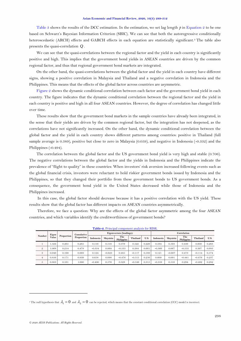
Table 2 shows the results of Equation 1. We extract the first two principal components whose eigenvalues are

greater than one. The correlation coefficient between the second principal component and the US government bond

yield (0.683) is higher than that between the first principal component and the US government bond yield (0.263).

The eigenvectors (loading coefficient) of the first principal component in all countries have positive values,

indicating that the first principal component has a symmetric effect among ASEAN countries. Moreover, the

eigenvector (loading coefficient) of the second principal component on the US government bond yield (0.661) is

higher than that of the first principal component (0.229). Thus, we identify the first principal component as regional

factor r

tf and the second principal component as global factor g

tf .


298


Table 3 shows the results of the DCC estimation. In the estimation, we set lag length p in Equation 2 to be one

based on Schwarz’s Bayesian Information Criterion (SBIC). We can see that both the autoregressive conditionally

heteroscedastic (ARCH) effects and GARCH effects in each equation are statistically significant.3 The table also

presents the quasi-correlation Q .

We can see that the quasi-correlations between the regional factor and the yield in each country is significantly

positive and high. This implies that the government bond yields in ASEAN countries are driven by the common

regional factor, and thus that regional government bond markets are integrated.

On the other hand, the quasi-correlations between the global factor and the yield in each country have different

signs, showing a positive correlation in Malaysia and Thailand and a negative correlation in Indonesia and the

Philippines. This means that the effects of the global factor across countries are asymmetric.

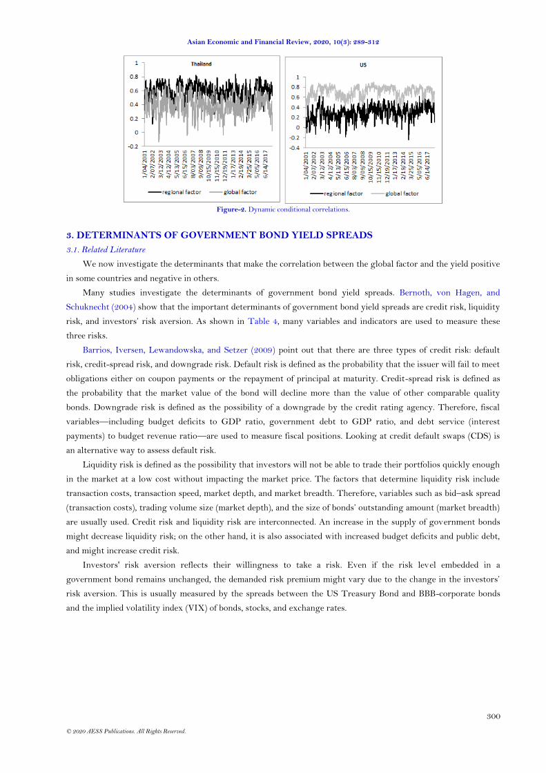
Figure 2 shows the dynamic conditional correlation between each factor and the government bond yield in each

country. The figure indicates that the dynamic conditional correlation between the regional factor and the yield in

each country is positive and high in all four ASEAN countries. However, the degree of correlation has changed little

over time.

These results show that the government bond markets in the sample countries have already been integrated, in

the sense that their yields are driven by the common regional factor, but the integration has not deepened, as the

correlations have not significantly increased. On the other hand, the dynamic conditional correlation between the

global factor and the yield in each country shows different patterns among countries: positive in Thailand (full

sample average is 0.389), positive but close to zero in Malaysia (0.059), and negative in Indonesia (-0.332) and the

Philippines (-0.494).

The correlation between the global factor and the US government bond yield is very high and stable (0.706).

The negative correlations between the global factor and the yields in Indonesia and the Philippines indicate the

prevalence of ―flight to quality‖ in these countries: When investors’ risk aversion increased following events such as

the global financial crisis, investors were reluctant to hold riskier government bonds issued by Indonesia and the

Philippines, so that they changed their portfolio from these government bonds to US government bonds. As a

consequence, the government bond yield in the United States decreased while those of Indonesia and the

Philippines increased.

In this case, the global factor should decrease because it has a positive correlation with the US yield. These

results show that the global factor has different impacts on ASEAN countries asymmetrically.

Therefore, we face a question: Why are the effects of the global factor asymmetric among the four ASEAN

countries, and which variables identify the creditworthiness of government bonds?

Table-2. Principal component analysis for RISK.

Number Eigen Value

Proportion Cumulative Proportion

Eigenvectors (loadings): Correlation

Indonesia Mayaisia The

Philippins Thailand U.S. Indonesia Mayaisia

The Philippins

Thailand U.S.

1 1.324 0.265 0.265 0.516 0.516 0.379 0.522 0.229 0.594 0.593 0.436 0.600 0.263

2 1.068 0.214 0.478 -0.354 0.064 -0.535 0.384 0.661 -0.366 0.067 -0.553 0.397 0.683

3 0.949 0.190 0.668 0.124 -0.623 0.485 -0.117 0.589 0.121 -0.607 0.473 -0.114 0.574

4 0.856 0.171 0.839 0.658 0.098 -0.476 -0.515 0.256 0.609 0.091 -0.441 -0.476 0.237

5 0.803 0.161 1.000 -0.400 0.576 0.328 -0.549 0.315 -0.359 0.516 0.294 -0.492 0.282

3 The null hypothesis that 1 0 and

2 0 can be rejected, which means that the constant conditional correlation (CCC) model is incorrect.


299


Table-3. Dynamic conditional correlation.

Indonesia Malaysia The Philippines Thailand

i ARCH (β1) 0.124*** 0.135*** 0.184*** 0.082***

(0.012) (0.010) (0.015) (0.005)

GARCH

(γ1) 0.870*** 0.876*** 0.831*** 0.916***

(0.013) (0.008) (0.013) (0.005)

fg ARCH (β1) 0.076*** 0.067*** 0.073*** 0.063***

(0.008) (0.007) (0.006) (0.006)

GARCH

(γ1) 0.907*** 0.917*** 0.912*** 0.921***

(0.009) (0.009) (0.008) (0.008)

fr ARCH (β1) 0.139*** 0.112*** 0.156*** 0.093***

(0.010) (0.008) (0.013) (0.007)

GARCH

(γ1) 0.858*** 0.881*** 0.844*** 0.900***

(0.009) (0.008) (0.012) (0.007)

Corr(i, fg) -0.311*** 0.047 -0.495*** 0.405***

(0.028) (0.034) (0.024) (0.027)

Corr(i, fr) 0.588*** 0.618*** 0.442*** 0.618***

(0.021) (0.022) (0.025) (0.020)

λ1 0.044*** 0.047*** 0.048*** 0.045***

(0.004) (0.003) (0.003) (0.003)

λ2 0.924*** 0.924*** 0.918*** 0.923***

(0.007) (0.006) (0.006) (0.005)

Note: † Standard errors are in parentheses. ‡ The asterisks *** denote significance at the 1% level.


300


Figure-2. Dynamic conditional correlations.

3. DETERMINANTS OF GOVERNMENT BOND YIELD SPREADS

3.1. Related Literature

We now investigate the determinants that make the correlation between the global factor and the yield positive

in some countries and negative in others.

Many studies investigate the determinants of government bond yield spreads. Bernoth, von Hagen, and

Schuknecht (2004) show that the important determinants of government bond yield spreads are credit risk, liquidity

risk, and investors’ risk aversion. As shown in Table 4, many variables and indicators are used to measure these

three risks.

Barrios, Iversen, Lewandowska, and Setzer (2009) point out that there are three types of credit risk: default

risk, credit-spread risk, and downgrade risk. Default risk is defined as the probability that the issuer will fail to meet

obligations either on coupon payments or the repayment of principal at maturity. Credit-spread risk is defined as

the probability that the market value of the bond will decline more than the value of other comparable quality

bonds. Downgrade risk is defined as the possibility of a downgrade by the credit rating agency. Therefore, fiscal

variables—including budget deficits to GDP ratio, government debt to GDP ratio, and debt service (interest

payments) to budget revenue ratio—are used to measure fiscal positions. Looking at credit default swaps (CDS) is

an alternative way to assess default risk.

Liquidity risk is defined as the possibility that investors will not be able to trade their portfolios quickly enough

in the market at a low cost without impacting the market price. The factors that determine liquidity risk include

transaction costs, transaction speed, market depth, and market breadth. Therefore, variables such as bid–ask spread

(transaction costs), trading volume size (market depth), and the size of bonds’ outstanding amount (market breadth)

are usually used. Credit risk and liquidity risk are interconnected. An increase in the supply of government bonds

might decrease liquidity risk; on the other hand, it is also associated with increased budget deficits and public debt,

and might increase credit risk.

Investors' risk aversion reflects their willingness to take a risk. Even if the risk level embedded in a

government bond remains unchanged, the demanded risk premium might vary due to the change in the investors’

risk aversion. This is usually measured by the spreads between the US Treasury Bond and BBB-corporate bonds

and the implied volatility index (VIX) of bonds, stocks, and exchange rates.


301


Table-4. Related literature: determinants of government bond spreads.

Author

Countries / Bench mark countries Variables Findings

Sample periods / Frequency

Bernoth et al. (2004)

13 EU countries/Germany, U.S.

(i) debt/GDP, (ii) fiscal balance/GDP (iii), debt service payments to total revenue ratios, (iv) corporate bond spread, (v)time to maturity of the government bond, (vi)country’s outstanding of government bonds/EU outstanding of government bonds, (vii) business cycle variable

Yield spreads of EU countries reflect positive default and liquidity risk premia. The default risk premium is positively affected by the debt and debt service ratios of the issuer country. Liquidity risk premia are reduced with EMU membership, which points to an increase in financial market integration.

1991-2002/annual

Manganelli and Wolswijk (2007)

10 euroa area countries (excl. Luxembourg)/Germany

(i) interaction term between main refinancing operations minimum bid rate and rating dummies(AA+, AA, AA-, A+ and A), (ii) AAA rating (liquidity premiums), (iii) country’s outstanding/euro area outstanding of government bonds

Spreads tend to be driven by the level of short-term interest rates. Sovereigns with lower credit ratings are forced to pay a higher credit risk premium, which means that market discipline still operating in EMU.

1999M1-2006M5/monthly

Barrios et al. (2009)

Austria, Belgium, Spain, France, Germany, Greece, Italy, Portugal

(i) CDS spread, (ii)bid-ask spread, (iii)risk aversion indicator, (iv) global financial crisis dummy

Euro area sovereign bond interest rates are strongly influenced by conditions in global financial markets. Domestic factors like liquidity and credit risk have become more important in the financial crisis to explain yield differentials.

2003M3 - 2009M4 / weekly

Haugh, Ollivaud, and Turner (2009)

Austria, Belgium, Finland, France, Greece, Italy, Netherlands, Portugal, Spain / Germany

(i) gross and net debt/GDP, (ii) debt service ratio, (iii) expected future fiscal deficits, (iv) corporate bond spread, (v) expected future public pension expenditures, (vi) country’s outstanding government bonds/euro-area total outstanding government bonds

Fiscal policies, particularly their effect on future deficits, and the debt service ratiohave an important role in explaining bond yield spreads.

2005Q4-2009Q2/semi-annual

Barbosa and Costa (2010)

10 euro area countries (excl. Luxembourg)/Germany

(i) CDS spread, (ii) fiscal balance/GDP, (iii) public debt /GDP, (iv)international invest position, (v) bid-ask spread, (vi) volumes available for trade, (vii)trading volume, (viii)first principal component of BBB corporate bond spreads, CDS indices and stock and bond markets implied

Government bond spreads can largely be explained by differences betweencreditworthiness of national governments, liquidity in domestic bond markets, as well as by the risk premium in international financial markets.

2007M1-2009M12 or 2010M5


302


volatilities

Author Countries / Bench mark countries Variables Findings Sample periods / Frequency

Bellas, Papaioannou, and Petrova (2010)

14 emerging market economies/U.S.

(i) external debt/GDP, (ii) interest payments on external debt/reserves, (iii) short-term debt/reserves, (iv) external debt amortization/reserves, (v) fiscal balance/GDP, (vi) current account/GDP, (vi)trade openness, (vii) financial stress index, (viii) U.S. 3-month Treasury bill rate and 10-year government bond yield, (ix) VIX, (x) political risk

Financial fragility is a more important determinant of spreads than fundamental indicators in the short run. On the other hand, fundamentals are significant determinants in the long run. In addition, other factors, such as political instability, corruption, and asymmetry of information may also affect the spread.

1997Q1-2009Q2/quarterly

Schuknecht, von Hagen, and Wolswijk (2010)

15 EU countries/Germany U.S.

(i) debt to GDP, (ii) fiscal balance/GDP, (iii), time to maturity, (iv) size of bond issue, (v) corporate bond spreads, (vi) short-time interest rate, (vii) interaction term between fiscal variables and turmoil and crisis dummy, (viii) country’s outstanding of government bonds/EU outstanding of government bonds, (ix) business cycle variable

Bond yield spreads can still largely be explained on the basis of economic principles during the crisis. Markets penalise fiscal imbalances much more strongly since the Lehman default in September 2008. In addition to fiscal deficits and debt,there is also a significant increase in the spread due to general risk aversion.

1999M1-2007M6

Belhocine and Dell’Erba (2013)

26 emerging market economies (i) VIX, (ii) international

reserves/GDP, (iii) CPI inflation, (iv)real GDP growth, (v)primary balance/GDP, (vi)public debt/GDP, (vii) money market interest rate, (viii) difference between the debt stabilizing primary balance and actual primart balance

Debt sustainability measured by the difference between the debt stabilizing primary balance and actual primary balance is a major determinant of spreads. Spreads become significantly more sensitive to debt sustainability as public debt increases.

1994-2011/semi-annual

Csonto and Ivaschenko (2013)

18 emerging market economies

(i) Economic Risk Rating, (ii) Financial Risk Rating, (iii) Political Risk Rating (from International Country Risk Guide), (iv)VIX, (v) U.S. Federal Funds rate

In the periods of severe market stress, such as during the intensive phase of the Eurozone debt crisis, global factors tend to drive changes in the spreads and the misalignment tends to increase in magnitude and its relative share in actual spreads.



303


Afonso, Arghyrou, and Kontonikas (2015)

10 euro area countries (excl. Luxembourg)/Germany

(i)lagged spreads, (ii) VIX, (iii) bid-ask spread, (iv)expected fiscal balance /GDP, (v) expected debt/GDP, (vi) real effective exchange, (vii) annual growth rate of industrial production, (viii) potential heterogeneity between periphery and core countries (principal components ob government bond yields spreads)

The determinants have changed significantly over time, and changes in the sensitivity of bond prices to fundamentals are also relevant to explain yields over the crisis period. More specifically, during the pre-crisis period macro- and fiscal-fundamentals are generally not significant in explaining spreads. By contrast, since summer 2007 the movements of macro- and fiscal- fundamentals explain spread movements well.


3.2. Empirical Methods

We employ the PMG method proposed by Pesaran, Shin, and Smith (1999). This model has several advantages

because it allows the short-run parameters to vary across countries while restricting long-run parameters to be

identical across countries. First, it assumes a dynamic model, which can capture the nature of the data. Second, it

imposes homogeneity among long-run coefficients, which leads to more stable estimates. Third, it allows the

separation of short-term dynamics and adjustment toward long-run equilibrium so that it can consider the

heterogeneity in short-run responses across countries.

We start with the ARDL (p, q, …, q) model:

, , , 1 , , 2 , ,

1 0 0

p q q

i t i i j i t j i j i t j i j t j i t

j j j

s s X Z

, (8)

where ,i ts denotes the government bond yield spread of country i, ,i tX and

tZ , 1 1k is the vector of the

country-specific variables expected to affect credit risk and liquidity risk, and 2 1k is the vector of the global

variables that are expected to reflect investors’ risk aversion, respectively. 1 ,i j and 2 ,i j are 1 1k and

2 1k

vector of coefficients. Equation 8 can be arranged to obtain the error correction equation:

1 1 1

* * * *

, , 1 1 , 2 , , 1 , , 2 ,

0 0 0

p q q

i t i i t i i i t i t i j i t j i j i t j i j t j it

j j j

s s X Z s X Z

, (9)

where

,

1

1p

i i j

j

,

*

1

1

ii p

ij

j

,

1 ,

1

1

,

1

1

q

i j

j

i p

i j

j

,

2 ,

1

2

,

1

1

q

i j

j

i p

i j

j

,

*

, ,

1

p

i j i m

m j

( 1, 1j p ), *

1 , 1 ,

1

q

i j i m

m j

and *

2 , 2 ,

1

q

i j i m

m j

( 1, 1j q )


304


By imposing homogeneity restrictions on the long-run coefficients (1 1i ,

2 2i ), Equation 9 can be

rewritten as

1 1 1

* * * *

, , 1 1 , 2 , , 1 , , 2 ,

0 0 0

p q q

i t i i t i i t t i j i t j i j i t j i j t j it

j j j

s s X Z s X Z

.(10)

In the analysis, we set lag length 1p q based on the SBIC. Thus, we estimate the following equation from

Equation 10,

* * *

, , 1 1 , 2 1 , 2i t i i t i i t t i i t i t its s X Z X Z

. (11)

First, we assume that the US government bond is risk-free, so we calculate the government bond yield spreads

as the premium paid by ASEAN countries over a US government bond with comparable maturities (10 years).

We adopt explanatory variables following the literature. We use the following country-specific variables as

,i tX : (i) government budget balance to GDP ratio (BB), (ii) public debt to GDP ratio (PD), (iii) government interest

payments on public debt to budget revenue ratio (PIP), and (iv) the expected depreciation rates of the exchange rate

in terms of local currency per US dollars (EX). The expected depreciation rates of the exchange rate are employed

to control for the effects of exchange rate fluctuations, approximated by ex-ante realized values.

For liquidity risk, we cannot obtain relevant variables such as bid–ask spread, the size of trading volumes, or

turnover rates. Therefore, we use the public debt to GDP ratio (PD) to measure not only credit risk but also

liquidity risk. If the coefficient on PD is estimated to be positive and significant, this will indicate that the effects of

credit risk dominate those of liquidity risk and vice versa.

For global variables tZ , which are expected to reflect investors’ risk aversion, we will extract the first principle

component of the following three variables: (i) the spreads between US Treasury Bonds and BBB-corporate bonds,

(ii) the implied volatility index (VIX) for US stocks, and (iii) the implied volatility index for yen–euro exchange

rates. We will call the first principal component ―RISK.‖

Note that we do not employ CDS data as credit risk variables because they would reflect the investors’

subjective assessment of credit risk. However, one of the aims of this study is to investigate whether bond market

integration would advance or obstruct investors’ ability or willingness to discriminate between the creditworthiness

of national fiscal policies. We will thus examine whether investors’ subjective assessment of credit risk reflects the

relevant fiscal fundamental variables precisely. Therefore, using CDS data would be tautological.

3.3. Empirical Results

3.3.1. Data

Our sample covers 2001Q1 to 2017Q4 with quarterly data.4

As explained above, we construct a variable for investors’ risk aversion by extracting the first principle

component of (i) the spreads between US Treasury Bonds and BBB-corporate bonds, (ii) the implied volatility index

of US stocks, and (iii) the implied volatility index of yen–euro exchange rates. We use daily data and then convert

them to quarterly data by taking the averages over each quarterly period. The cumulative contribution rate of the

first principal component is above 80%, and three eigenvectors (factor-loadings) are about 0.6. Figure 3 displays the

4 In some countries, fiscal variables are available only from annual data. In those cases, we follow the Chow and Lin (1971) method of interpolating from annual to

quarterly data. For example, the annual public debt is interpolated to a quarterly series by using the quarterly budget balance as the related variable.


305


annual data for BB, PD, and PIP and quarterly data for RISK. The data are from International Financial Statistics

(IMF) and Economic Intelligence Unit.

Figure-3. Explanatory variables.

Source: International Financial Statistics (IMF) and Economic Intelligence Unit.

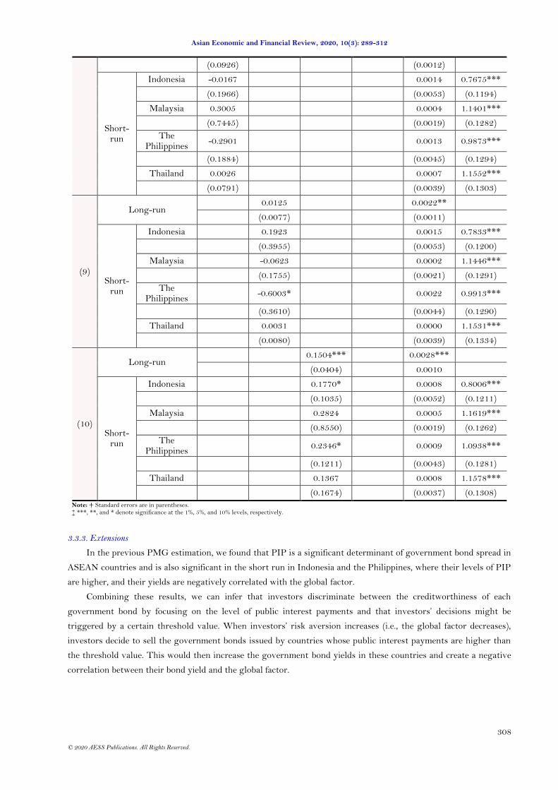
3.3.2. Empirical Results

Table 5 shows the results of the PMG estimation of Equation 11. The table shows that BB is not a significant

determinant in all specifications and that PD is also not significant except for specification (2) in the long-run.


306


Contrariwise, PIP has positive and significant effects on government bond yield in the long-run. This means that

PIP is an important determinant of government bond spreads in the four ASEAN countries. These results are

consistent with Bernoth et al. (2004) who find that fiscal imbalances are better captured by a measure of debt

service than either the deficit to GDP ratio or the debt to GDP ratio. Moreover, PIP is positive and significant in

Indonesia and the Philippines in the short run (in specifications [4] and [10]). As shown in Figure 3, PIP levels are

higher in Indonesia and the Philippines than in the other two countries. Therefore, the government bond markets

in the sample countries have maintained market discipline in the sense that investors discriminate between the

creditworthiness of each country by focusing on the public interest payments. These results might offer insights

into why the effects of the global factor are asymmetric among the ASEAN countries and why the correlation

between the global factor and the government bond yield are negative in Indonesia and the Philippines. The

investors’ risk aversion (RISK) is positive and significant for all specifications, indicating that, following events that

increased investors’ risk aversion, investors were reluctant to hold more risky assets and thus changed their

portfolios from ASEAN countries’ government bonds to those of advanced countries such as the United States. This

is known as ―flight to quality.‖

Table-5. Pooled mean group estimation.

BB PD PIP EXD RISK EC

(1)

Long-run 0.0631 0.0080 0.1332*** 0.0029 0.0023*

(0.1016) (0.0089) (0.0506) (0.0541) (0.0012)

Short-run

Indonesia -0.0497 0.0089 0.1808* 0.0332 0.0005 0.7811***

(0.2724) (0.5472) (0.1074) (0.0773) (0.0053) (0.1283)

Malaysia 0.3558 -0.1062 0.4729 -0.0469 -0.0002 1.2244***

(0.7440) (0.1810) (0.9186) (0.0568) (0.0022) (0.1379)

The Philippines

-0.2296 -0.6394* 0.1076 0.2702* 0.0005 0.8685***

(0.2802) (0.3656) (0.1953) (0.1381) (0.0041) (0.1453)

Thailand -0.1012 -0.0336 0.6090* 0.0312 -0.0004 1.0980***

(0.2920) (0.0323) (0.3643) (0.0915) (0.0039) (0.1340)

(2)

Long-run 0.0559 0.0150*

0.0082 0.0021*

(0.1027) (0.0083) (0.0553) (0.0013)

Short-run

Indonesia -0.1114 0.3475 0.0325 0.0014 0.7813***

(0.2755) (0.5571)

(0.0788) (0.0054) (0.1277)

Malaysia 0.2611 -0.0685

-0.0393 -0.0001 1.1916

(0.7609) (0.1795)

(0.0565) (0.0022) (0.1394)

The Philippines

-0.3459* -0.7886**

0.3247** 0.0009 0.7709***

(0.1834) (0.3596)

(0.1353) (0.0042) (0.1362）

Thailand -0.2421 -0.0265

0.0674 0.0003 1.1329***

(0.2906) (0.0329) (0.0917) (0.0040) (0.1333)

(3)

Long-run 0.0179

0.1518*** 0.0136 0.0024**

(0.0944) (0.0449) (0.0539) (0.0012)

Short-run

Indonesia -0.0660 0.1879* 0.0363 0.0006 0.7834***

(0.1976)

(0.1065) (0.0771) (0.0052) (0.1264)

Malaysia 0.3805

0.2274 -0.0423 0.0001 1.2151***

(0.7376)

(0.8695) (0.0562) (0.0021) (0.1368)

The Philippines

-0.1727

0.0861 0.2952** 0.0009 0.9359***

(0.2834)

(0.1982) (0.1400) (0.0042) (0.1439)


307


Thailand 0.1713

0.5458 0.0457 0.0002 1.1108***

(0.1304)

(0.3580) (0.0910) (0.0039) (0.1322)

(4)

Long-run 0.0050 0.1422*** 0.0102 0.0026**

(0.0085) (0.0486) (0.0540) (0.0010)

Short-run

Indonesia -0.0845 0.1795* 0.0319 0.0006 0.7796***

(0.3972) (0.1064) (0.0768) (0.0052) (0.1279)

Malaysia -0.0734 0.4463 -0.0457 -0.0002 1.2188***

(0.1777) (0.9191) (0.0559) (0.0022) (0.1369)

The Philippines

-0.5588 0.2498** 0.2619* 0.0004 0.8942***

0.3639 (0.1244) (0.1383) (0.0041) (0.1447)

Thailand -0.0212 0.6594* 0.0365 -0.0005 1.1018***

(0.0142) (0.3496) (0.0908) (0.0038) (0.1330)

(5)

Long-run -0.0307

0.0249 0.0020*

(0.0948) (0.0553) (0.0012)

Short-run

Indonesia -0.0295 0.0432 0.0014 0.7467***

(0.1984)

(0.0787) (0.0054) (0.1234)

Malaysia 0.1902

-0.0290 0.0002 1.1769***

(0.7540)

(0.0558) (0.0020) (0.1371)

The Philippines

-0.2469

0.3739*** 0.0013 0.8178***

(0.1788)

(0.1378) (0.0043) (0.1375)

Thailand 0.0034

0.0786 0.0011 1.1433***

(0.0797) (0.0909) (0.0039) (0.1304)

BB PD PIP EXD RISK EC

(6)

Long-run 0.0123 0.0144 0.0023**

(0.0077) (0.0552) (0.0011)

Short-run

Indonesia 0.1736 0.0311 0.0014 0.7673***

(0.3994)

(0.0786) (0.0054) (0.1255)

Malaysia -0.0399

-0.0377 0.0000 1.1850***

(0.1764)

(0.0556) (0.0022) (0.1383)

The Philippines

-0.5146

0.3580** 0.0020 0.8260***

(0.3466)

(0.1381) (0.0042) (0.1383)

Thailand 0.0034

0.0775 0.0004 1.1452***

(0.0080) (0.0913) (0.0039) (0.1331)

(7)

Long-run 0.1537*** 0.0181 0.0027***

(0.0436) (0.0536) (0.0009)

Short-run

Indonesia 0.1788* 0.0321 0.0008 0.7842***

(0.1036) (0.0760) (0.0052) (0.1266)

Malaysia 0.2731 -0.0428 0.0001 1.2139***

(0.8686) (0.0553) (0.0020) (0.1361)

The Philippines

0.1903 0.2865** 0.0010 0.9487***

(0.1197) (0.1397) (0.0042) (0.1429)

Thailand 0.1297 0.0761 0.0011 1.1476***

(0.1673) (0.0890) (0.0037) (0.1308)

(8) Long-run -0.0356 0.0020*


308


(0.0926) (0.0012)

Short-run

Indonesia -0.0167

0.0014 0.7675***

(0.1966)

(0.0053) (0.1194)

Malaysia 0.3005

0.0004 1.1401***

(0.7445)

(0.0019) (0.1282)

The Philippines

-0.2901

0.0013 0.9873***

(0.1884)

(0.0045) (0.1294)

Thailand 0.0026

0.0007 1.1552***

(0.0791) (0.0039) (0.1303)

(9)

Long-run 0.0125

0.0022**

(0.0077) (0.0011)

Short-run

Indonesia 0.1923 0.0015 0.7833***

(0.3955)

(0.0053) (0.1200)

Malaysia

-0.0623

0.0002 1.1446***

(0.1755)

(0.0021) (0.1291)

The Philippines

-0.6003*

0.0022 0.9913***

(0.3610)

(0.0044) (0.1290)

Thailand

0.0031

0.0000 1.1531***

(0.0080) (0.0039) (0.1334)

(10)

Long-run 0.1504***

0.0028***

(0.0404) 0.0010

Short-run

Indonesia 0.1770* 0.0008 0.8006***

(0.1035)

(0.0052) (0.1211)

Malaysia

0.2824

0.0005 1.1619***

(0.8550)

(0.0019) (0.1262)

The Philippines

0.2346*

0.0009 1.0938***

(0.1211)

(0.0043) (0.1281)

Thailand

0.1367

0.0008 1.1578***

(0.1674) (0.0037) (0.1308)

Note: † Standard errors are in parentheses. ‡ ***, **, and * denote significance at the 1%, 5%, and 10% levels, respectively.

3.3.3. Extensions

In the previous PMG estimation, we found that PIP is a significant determinant of government bond spread in

ASEAN countries and is also significant in the short run in Indonesia and the Philippines, where their levels of PIP

are higher, and their yields are negatively correlated with the global factor.

Combining these results, we can infer that investors discriminate between the creditworthiness of each

government bond by focusing on the level of public interest payments and that investors’ decisions might be

triggered by a certain threshold value. When investors’ risk aversion increases (i.e., the global factor decreases),

investors decide to sell the government bonds issued by countries whose public interest payments are higher than

the threshold value. This would then increase the government bond yields in these countries and create a negative

correlation between their bond yield and the global factor.


309


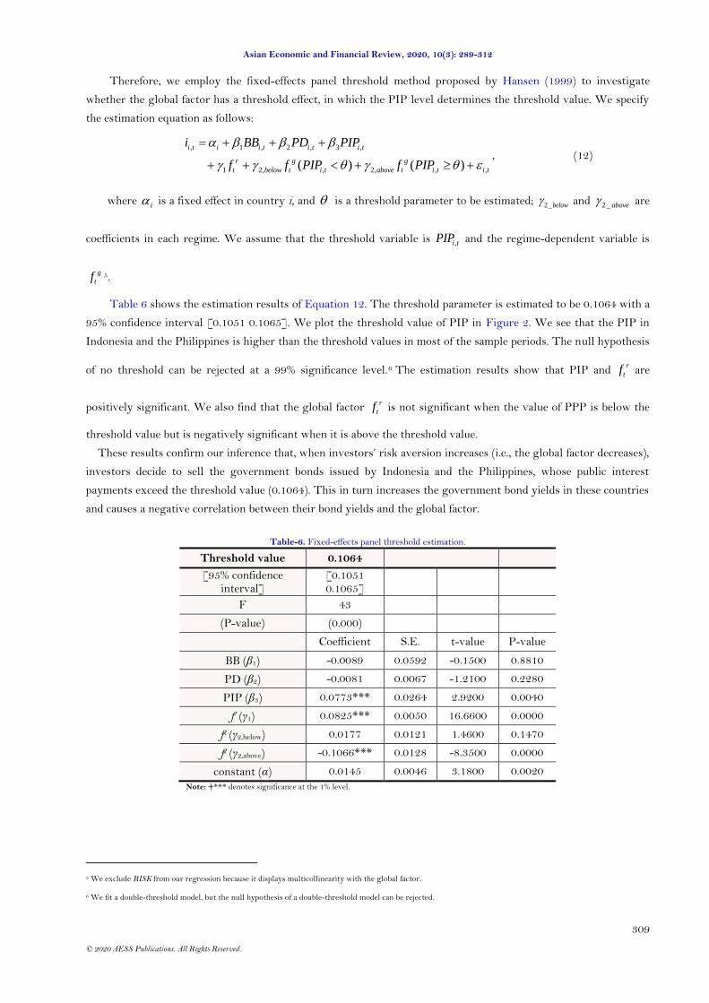
Therefore, we employ the fixed-effects panel threshold method proposed by Hansen (1999) to investigate

whether the global factor has a threshold effect, in which the PIP level determines the threshold value. We specify

the estimation equation as follows:

, 1 , 2 , 3 ,

1 2, , 2, , ,( ) ( )

i t i i t i t i t

r g g

t below t i t above t i t i t

i BB PD PIP

f f PIP f PIP

, (12)

where i is a fixed effect in country i, and is a threshold parameter to be estimated; 2 _ below and 2 _ above are

coefficients in each regime. We assume that the threshold variable is ,i tPIP and the regime-dependent variable is

g

tf5.

Table 6 shows the estimation results of Equation 12. The threshold parameter is estimated to be 0.1064 with a

95% confidence interval [0.1051 0.1065]. We plot the threshold value of PIP in Figure 2. We see that the PIP in

Indonesia and the Philippines is higher than the threshold values in most of the sample periods. The null hypothesis

of no threshold can be rejected at a 99% significance level.6 The estimation results show that PIP and r

tf are

positively significant. We also find that the global factor r

tf is not significant when the value of PPP is below the

threshold value but is negatively significant when it is above the threshold value.

These results confirm our inference that, when investors’ risk aversion increases (i.e., the global factor decreases),

investors decide to sell the government bonds issued by Indonesia and the Philippines, whose public interest

payments exceed the threshold value (0.1064). This in turn increases the government bond yields in these countries

and causes a negative correlation between their bond yields and the global factor.

Table-6. Fixed-effects panel threshold estimation.

Threshold value 0.1064

[95% confidence interval]

[0.1051 0.1065]

F 43

(P-value) (0.000)

Coefficient S.E. t-value P-value

BB (β1) -0.0089 0.0592 -0.1500 0.8810

PD (β2) -0.0081 0.0067 -1.2100 0.2280

PIP (β3) 0.0773*** 0.0264 2.9200 0.0040

fr (γ1) 0.0825*** 0.0050 16.6600 0.0000

fg (γ2,below) 0.0177 0.0121 1.4600 0.1470

fg (γ2,above) -0.1066*** 0.0128 -8.3500 0.0000

constant (α) 0.0145 0.0046 3.1800 0.0020

Note: †*** denotes significance at the 1% level.

5 We exclude RISK from our regression because it displays multicollinearity with the global factor.

6 We fit a double-threshold model, but the null hypothesis of a double-threshold model can be rejected.


310


4. CONCLUSIONS

We examined whether the government bond markets in four ASEAN countries are integrated. We employed

the approximate dynamic factor model to decompose the yields in four ASEAN countries and the United States into

the global factor, the regional factor, and the idiosyncratic shock and then investigated the time-varying

correlations between each factor and the yield in each country using the DCC method. Our results show that the

government bond markets in the sample countries are integrated in the sense that their yields are driven by a

common regional factor, but the integration has not intensified, as the correlations have not increased. We also find

that the global factor has asymmetric effects on government bond yields in the four ASEAN countries: The

correlation between the global factor and the government bond yields is positive in Malaysia and Thailand but

negative in Indonesia and the Philippines.

Based on these results, we next investigate the determinants of government bond spreads using PMG

estimation methods, which allow heterogeneity in the short-run responses across countries. We find that public

interest payments are the most important determinant and have positive and significant effects on government

bond yields in the long run. They also have positive and significant effects in the short run in Indonesia and the

Philippines, where public interest payments are higher and their yields are negatively correlated with the global

factor. We also find that investors’ risk aversion has positive and significant effects, indicating flight to quality.

We then use the fixed-effects panel threshold method to investigate whether there exists a threshold that

depends on public interest payments. We find that the global factor is not significant when public interest payments

are below the threshold value but is negatively significant when they are above the threshold.

Combining these results, we can conclude that market discipline has been operating in the four ASEAN

government bond markets in the sense that investors discriminate between the creditworthiness of the

governments’ bonds by focusing on the public interest payments.

Funding: This study received no specific financial support. Competing Interests: The authors declare that they have no competing interests. Acknowledgement: Both authors contributed equally to the conception and design of the study.

REFERENCES

Adam, K., Jappeli, T., Menichini, A., Padula, M., & Pagano, M. (2002). Analyse, compare, and apply alternative indicators and

monitoring methodologies to measure the evolution of capital market integration in the European Union. Report to

European Commissions.

Afonso, A., Arghyrou, M. G., & Kontonikas, A. (2015). The determinants of sovereign bond yield spreads in the EMU. ECB

Working Paper No.1781.

Baele, L., Ferreando, A., Hördahl, P., Krylova, E., & Monnet, C. (2004). Measuring financial integration in the Euro area. ECB

Occasional Paper Series No.14. European Central Bank.

Barbosa, L., & Costa, S. (2010). Determinants of sovereign bond yield spreads in the Euro area in the context of the economic

and financial crisis. Banco de Portugal Working Paper 22/2010.

Barrios, S., Iversen, P., Lewandowska, M., & Setzer, R. (2009). Determinants of intra-Euro area government bond spreads

during the financial crisis. European Economy, Economic Papers No. 388.

Belhocine, N., & Dell’Erba, S. (2013). The impact of debt sustainability and the level of debt on emerging markets spreads. IMF

Working Paper 2013/93. Retrieved from: https://doi.org/10.5089/9781484382769.001.

Bellas, D., Papaioannou, M. G., & Petrova, I. (2010). Determinants of emerging market sovereign bond spreads: Fundamentals

vs financial stress. IMF Working Paper 2010/281. Retrieved from: https://doi.org/10.5089/9781455210886.001.

Bernoth, K., von Hagen, J., & Schuknecht, L. (2004). Sovereign risk premia in the European government bond market. ECB

Working Paper No. 369.


311


Calvi, R. (2010). Assessing financial integration: A comparison between Europe and East Asia. European Economy, Economic

Papers 423.

Chow, G. C., & Lin, A. (1971). Best linear unbiased distribution and extrapolation of economic time series by related series.

Review of Economic and Statistics, 53(4), 372-375. Available at: https://doi.org/10.2307/1928739.

Clare, A. D., Maras, M., & Thomas, S. H. (1995). The integration and efficiency of international bond markets. Journal of Business

Finance & Accounting, 22(2), 313-322. Available at: https://doi.org/10.1111/j.1468-5957.1995.tb00687.x.

Click, R. W., & Plummer, M. G. (2005). Stock market integration in ASEAN after the Asian financial crisis. Journal of Asian

Economics, 16(1), 5-28. Available at: https://doi.org/10.1016/j.asieco.2004.11.018.

Csonto, B., & Ivaschenko, I. (2013). Determinants of sovereign bond spreads in emerging markets: Local fundamentals and

global factors vs. ever-changing misalignments. IMF Working Paper 2013/164. Retriieved from:

https://doi.org/10.5089/9781475573206.001.

Engle, R. F. (2002). Dynamic conditional correlation: A simple class of multivariate GARCH Models. Journal of Business and

Economic Statistics, 20(3), 339–350. Available at: https://doi.org/10.1198/073500102288618487.

Haldane, A. G., & Hall, S. G. (1991). Sterling's relationship with the dollar and the deutschemark: 1976-89. The Economic Journal,

101(406), 436-443. Available at: https://doi.org/10.2307/2233550.

Hansen, B. E. (1999). Threshold effects in non-dynamic panels: Estimation, testing, and inference. Journal of Econometrics, 93(2),

345-368. Available at: https://doi.org/10.1016/s0304-4076(99)00025-1.

Haugh, D., Ollivaud, P., & Turner, D. (2009). What drives sovereign risk premiums? An analysis of recent evidence from the

Euro area. OECD Economic Development Working Papers No.718.

Kasa, K. (1992). Common stochastic trends in international stock markets. Journal of monetary Economics, 29(1), 95-124. Available

at: https://doi.org/10.1016/0304-3932(92)90025-w.

Kim, S.-J., Lucey, B. M., & Wu, E. (2006). Dynamics of bond market integration between established and accession European

Union countries. Journal of International Financial Markets, Institutions and Money, 16(1), 41-56. Available at:

https://doi.org/10.1016/j.intfin.2004.12.004.

Manganelli, S., & Wolswijk, G. (2007). Market discipline, financial integration and fiscal rules: What drives spreads in the Euro

areas government bond market? ECB Working Paper No.745. Manning, Neil. 2002. ―Common trends and

convergence? South East Asia equity markets, 1988–1999. Journal of International Money and Finance, 21(2), 183–202.

Manning, N. (2002). Common trends and convergence? South East Asian equity markets, 1988–1999. Journal of International

Money and Finance, 21(2), 183-202. Available at: https://doi.org/10.1016/s0261-5606(01)00038-9.

Mills, T. C., & Mills, A. G. (1991). The international transmission of bond market movements. Bulletin of Economic Research,

43(3), 273-281. Available at: https://doi.org/10.1111/j.1467-8586.1991.tb00496.x.

Park, C. (2013). Asian capital market integration: Theory and evidence. ADB Economics Working Paper Series 351. Asian

Development Bank.

Pesaran, M., Shin, H., & Smith, Y. R. P. (1999). Pooled mean group estimation of dynamic heterogeneous panels. Journal of the

American Statistical Association, 94(446), 621–634.

Rangvid, J. (2001). Increasing convergence among European stock markets? A recursive common stochastic trends analysis.

Economics Letters, 71(3), 383-389. Available at: https://doi.org/10.1016/s0165-1765(01)00361-5.

Schuknecht, L., von Hagen, J., & Wolswijk, G. (2010). Government bond risk premiums in the EU revisited: The impact of the

financial crisis. ECB Working Paper No.1152.

Serletis, A., & King, M. (1997). Common stochastic trends and convergence of European Union stock markets. The Manchester

School, 65(1), 44-57. Available at: https://doi.org/10.1111/1467-9957.00042.

Stock, J. H., & Mark, W. W. (1998). Diffusion indexes. NBER Working Paper, No. 6702.

Stock, J. H., & Mark, W. W. (2002a). Forecasting using principal components from a large number of predictors. Journal of

American Statistical Association, 97(460), 1167–1179.


312


Stock., J. H., & Mark, W. W. (2002b). Macroeconomic forecasting using diffusion Indexes. Journal of Business & Economic

Statistics, 20(2), 147–162.

Tsukuda, Y., Shimada, J., & Miyakoshi, T. (2017). Bond market integration in East Asia: Multivariate GARCH with dynamic

conditional correlations approach. International Review of Economics & Finance, 51, 193-213. Available at:

https://doi.org/10.1016/j.iref.2017.05.013.

Vo, X. V. (2009). International financial integration in Asian bond markets. Research in International Business and Finance, 23(1),

90-106.

Yu, I., Fung, L., & Tam, C. (2007). Assessing bond market integration in Asia. Working Paper 10/2007, Hong Kong Monetary

Authority.

Views and opinions expressed in this article are the views and opinions of the author(s), Asian Economic and Financial Review shall not be responsible or answerable for any loss, damage or liability etc. caused in relation to/arising out of the use of the content.

asian economic and social society - government bond market integration in asean3)-289-312.pdf ·...

Documents