asafes2: a novel, neuro-fuzzy architecture for fuzzy computing, based on functional reasoning

E L S E V I E R Fuzzy Sets and Systems 83 (1996) 63-84

ZZ'¥ sets and systems

ASAFES2: a novel, neuro-fuzzy architecture for fuzzy computing, based on functional reasoning

Konstantinos C. Zikidis, Athanasios V. Vasilakos* Department of Computer Science. Hellenic Air Force Academy, Dekelia TGA 1010, Athens, Greece

Received January 1995

Abstract

The functional reasoning or Takagi-Sugeno fuzzy reasoning method is a very promising approach to the task of multi-variable, non-linear function approximation, and the design of a fuzzy model and fuzzy controller. The proposed architecture, ASAFES2, is a neuro-fuzzy function approximator, and is the first attempt to combine this reasoning method with stochastic reinforcement learning. It can "learn" a function to a high degree of accuracy, at a very great speed, and furthermore, expresses it in a set of linear relations. The main ideas are the fuzzy partitioning of the input space into fuzzy subspaces (each corresponding to a possible fuzzy rule), and the use of a separate neural unit for every fuzzy subspace, in order to calculate the optimum consequence parameters. Simulation results prove its superiority over back-propagation in simple non-linear function approximation tasks, and over all previous approaches to the Box and Jenkins gas furnace modelling. Comparisons are also made with Generalized Radial Basis Function Networks. Finally, ASAFES2, as a building block in a learning fuzzy logic controller, is applied to the well-known cart-pole stabilization problem, with satisfactory results. A new, flexible membership function is also presented.

Keywords: Functional reasoning; Stochastic reinforcement learning; Function approximation; Fuzzy modelling; Gener- alized Radial Basis Function Networks; Delayed reinforcement; Temporal difference methods

I. Introduction

Fuzzy logic and neural networks are mathemat - ical approaches towards the human way of think-

*Corresponding author. Address: Computer Science Insti- tute, Foundation of Research and Technology - Hellas (FORTH), University of Crete, P.O. Box 1385, Heraklion, Crete, Greece.

~5 ASAFES stands for Adaptive Stochastic Algorithm for Fuzzy computing/function EStimation. "Asafes" means "fuzzy'" in Greek

ing and learning. Man does not simply tolerate the vagueness and imprecision of the facts and (generally) the data he uses in his decision making, but he subconsciously exploits them. He keeps in mind, along with his data, their importance, randomness and fuzziness, and, using his massively parallel distributed processing brain, he spontaneously comes to a result. The microstructure the h a r d w a r e - of the human brain inspired the neural network re- searchers and led them to the design of algori thms employing many, simple processing units, which have the ability to learn from examples. On the

0165-0114/96/$15.00 Copyright ~ 1996 Elsevier Science B.V. All rights reserved SSDI 0165-01 14 (95 )00296-0

64 K.C. Zikid&, A.V. Vasilakos / Fuzz)' Sets" and Systems 83 (1996) 63-84

other hand, the effectiveness and simplicity of the higher level thinking, which is always based on more or less fuzzy data, also stimulated the research community and led to the development of a theory which could deal with fuzziness: the fuzzy set theory.

Since Zadeh established a new direction in mathematical reasoning [34, 35], a great number of studies on fuzzy logic have been reported. Mam- dani was the first who applied fuzzy set theory to control [15], possibly the most important application of fuzzy logic. Various fuzzy reasoning methods have also been proposed [16]. Most of them are based on the classical min-max-centroidal method or a simplified version of it [37]. This reasoning is very similar to the human inference and can be expressed with the use of linguistic variables. However, when applied to multi-dimensional reasoning, it often leads to rule explosion, since, in most of the cases, at least 5 linguistic values have to be assigned to each linguistic variable. To reduce the number of implications, Takagi and Sugeno proposed the functional reasoning [24]. The main difference between this method and the min-max-centroidal method lies in the consequence part, where there is a linear input/output relation instead of a fuzzy set. A simple weighted average is used for the calculation of the output, instead of the compositional rule of inference.

In this paper the authors propose the architecture ASAFES2, a fuzzy neural network, integrating Sugeno's fuzzy reasoning method with the learning ability of neural networks. In a few words, the operation of ASAFES2 comprises the following steps: In the beginning of training, the input space is partitioned into fuzzy subspaces. On the way, ASAFES2 forms a fuzzy rule for every fuzzy subspace (if encountered), consisting of a premise part using Larsen's method [16], and a consequence part, which is a linear input/output relation. The coefficients of this linear relation can be calculated with a variety of neural net training algorithms. Finally, the output value is a weighted average of the outputs produced by the activated fuzzy rules.

ASAFES2 is based on the simple idea that "if a problem is too large to be solved, cut it into smaller ones". If a single or multi-variable function cannot be approximated satisfactorily with one

linear input/output equation, then its input variable space has to be divided in smaller, overlapping fuzzy subspaces, where a learning unit tries to establish an appropriate linear relation. In this way, the problem of learning is simplified: since linear units are employed, any simple algorithm can be used e.g. the Least Mean Square algorithm (LMS), with no need for calculating and propagating deriv- atives (as with back-prop) and only a linear approximation has to be learned for each region of the input space, which enables quite fast convergence. The final output is calculated by averaging the outputs produced from these relations. ASAFES2 may seem similar to the Generalized Radial Basis Function Networks (GRBFN) [9], even though their approach is from a different perspective. Their main differences are in the output function of the hidden neurons (in the GRBFN it is a constant, in ASAFES2 an input/output relation) and in the input space transformation (in the GRBFN it is usually a set of Gaussian functions while in ASAFES2 it is a set of fuzzy implications).

So, ASAFES2 can primarily be used for real- valued function approximation. It can learn a non- linear, multi-variable function through a set of input patterns. Furthermore, ASAFES2 expresses the learned function in an understandable and workable form of linear relations, enabling us to intervene, knowing "what is happening" into the net. For example, we can easily incorporate prior knowledge. Generally, this is one of the main advantages of fuzzy systems over neural networks: neural nets are treated as black boxes and the learned function cannot be expressed in a useful way, while fuzzy systems were built to express and exploit human knowledge.

Seeing ASAFES2 from another point of view, it appears to be a very powerful tool for fuzzy modelling. System modelling may be considered as a task of function approximation: the function that esti- mates the output of a system from its inputs (and previous inputs/outputs if it is a dynamical system) has to be learned from numerical input/output data. In general, fuzzy modelling can be defined as an approach to build the model of a system using fuzzy implications, and it is one of the most important applications of fuzzy set theory. It is a simple and efficient way to state mathematically the

K.C Zikidis, A.V. Vasilakos /Fuzzy Sets and Systems 83 (1996) 63-84 65

behaviour of a system, and, if the reasoning method allows it, express it also in a linguistic form.

However, ASAFES2 is intended to be used in control tasks; therefore reinforcement learning was chosen as the kind of training for testing, even in the function approximation tasks. Algorithms of this kind conduct a stochastic search of the output space, using only an approximate indication of the "correctness" of the output value they produced in ever iteration, which is a scalar called reinforcement [1-4, 11, 14, 28]. In the general case, this indication might be only a "good"/"bad" signal. Even worse, a "bad" signal might come after a sequence of actions, making impossible the direct assessment of each separate action (credit assignment problem). Reinforcement learning algorithms require less information compared to the supervised learning ones, e.g., LMS, back-prop [19], which are given with every input pattern the desired output pattern. In some tasks, where it is hard or expensive to obtain a priori information, reinforcement learning is more suitable than supervised learning. The training algorithm used in the function approximation tasks is the ANASA II algorithm [28,29]. ANASA stands for Adaptive Neural Algorithm of Stochastic Activation and is a simple, quite fast and reliable reinforcement learning algorithm.

A scheme like the Adaptive Heuristic Critic [3, 23], employing ASAFES2 as a building block, can be used to deal with control tasks where min- imal reinforcement is available [3]. A "critic" element, taking into consideration the state of the system under control, transforms the external, "raw" reinforcement signal, supplied by the environment, into a heuristic reinforcement of higher-level information. This internal reinforcement is used by the "actor" element, which shares the same inputs with the "critic" and is the one actually controlling the system. The idea of reinforcement learning in fuzzy logic control systems is not new [4, 14].

The performance of ASAFES2 is validated through simulation. It is trained with ANASA II through noise-free and noisy data to approximate a static non-linear function. It is compared with a feedforward neural network with one or two hidden layers, trained by a classic algorithm (back- prop with momentum), and found to be un-

doubtedly superior in every aspect. Preliminary results for this task appeared in [32]. It is also compared with Generalized Radial Basis Function Networks [9], with 16, 25 and 36 hidden units, with fixed centres, exhibiting very good performance, especially in terms of computational effort. Another task is presented, which uses the data from the Box and Jenkins gas furnace [6], a famous dynamical system example. Comparisons are made with earlier approaches, and again ASAFES2 is proved to be superior and more practical. Finally, ASAFES2 in an actor-critic configuration, using only a failure information, learns to stabilize the well-known cart-pole system, an inherently un- stable system.

ASAFES2 is an extension of our previous work ASAFES [31]. ASAFES is also a reinforcement learning algorithm, but is based on the classical fuzzy reasoning method (min-max-centroidal). Each possible fuzzy rule employs a separate Stochastic Estimator Learning Automaton (SELA [30]), to determine its consequence fuzzy set and regression analysis is used for the calculation of the corresponding rule weight (significance).

The rest of the paper is organized as follows: in the next two sections, the Sugeno reasoning method and the operation of a single neuron, along with the ANASA II algorithm, are presented. In Section 4 is the analytical presentation of ASAFES2 and in Section 5 is a brief presentation of the AHC scheme. In Section 6 is the simulation procedure and results. Section 7 is the conclusion.

2. The Takagi-Sugeno fuzzy reasoning method

The membership function of a fuzzy set A is denoted/~a(x) • The term "fuzzy rule" will be used throughout the paper, instead of "fuzzy process law" or "fuzzy implication". The functional reasoning method will be described here as it was originally presented by Takagi and Sugeno in [24].

Let #A(X) be the membership function or com- patibility degree of x in the fuzzy set A. The truth value of the proposition "Xl is A and xz is B" was expressed by:

Ixx is A and x2 is B[ = #a(Xa)ApB(X2).

6 6 K.C. Zikidis, A. IC Vasilakos / Fuzz ' Sets" and Systems 83 (1996) 63 84

The format of a fuzzy rule was:

R: if xl is A~ and ... and Xk is Ak

t h e n y = p 0 + p x . x l + ... + p k ' X k ,

where x l . . . . . Xk are the input variables and appear in the premise part and also in the consequence part, y is the output variable whose value is to be inferred and A1 . . . . . Ak the fuzzy sets defining the fuzzy subspace in which the fuzzy rule R is activated and produces an output. If a fuzzy set Ai in the premise is equal to the universe of discourse of xi, then this term is omitted.

If there is a knowledge base of N fuzzy rules R~, i = 1 . . . . . N, and we are given the input values:

X 1 : X'(, X 2 = X22, . . . , X k = Xk ,

then the output of every fuzzy rule Ri is calculated from the equation:

• " ' i . a . Y' = P'o + p'lx~ + "" + pkXk.

The truth value of the proposition y = y~ (or the firing strength of the rule R~) is:

lY = yi[ = Ix~ is A1 and ... and x~' is Akl

= ~ ,A, (x~) / , . . . ~ , ~,A~(x~).

The final value of the output variable, inferred from the N fuzzy rules, is the average of all yi weighted by the corresponding firing strengths l Y = Yil:

ou tpu t = ly = y i [ . yi 2 ly = yi l . i = 1 i 1

It has been proved in [7] that controllers using Sugeno's inference method, under certain modifications (Sugeno-type controllers), are universal approximators. This means that they can approximate any given function to any degree of accuracy. (The same author argues that regular fuzzy neural nets are not universal approximators, while neural networks are [8]. Also see [27].) However, the main advantage of this method is that the number of the fuzzy rules required is drastically reduced - a very important fact in multi-dimensional reasoning. Furthermore, the division of the input space into fuzzy subspaces makes feasible the application of a linear I/O relation. This enables us to exploit the advantages of linearity. The optimum parameter

identification can be made with a variety of methods, e.g. LMS, as was originally proposed, or with the use of reinforcement learning, as in the proposed scheme. In addition, it simplifies the design of a controller: a control rule can be easily derived with the aid of linear systems theory, for each subsystem, and the combination of the fuzzy control rules will form the fuzzy controller [21, 25].

3. The operation of a single neuron in ASAFES2 and the modified ANASA II updating rule

3.1. General description o f a s ingle neuron

Each neural unit has k + 1 input variables: x0, xl . . . . . Xk, and the corresponding k + 1 weights: w0, wl . . . . . wk. The input Xo is by default set to 1 and, in this way, the weight w0 acts as a threshold (bias) weight. In the beginning of training, the weights are set to or near zero. Suppose that at time step n (or iteration n), the input pattern x;" is presented to the neuron input. It is reminded that Xo = 1, so

x (n ) = [1, x~, x2, "~ . . . , x~] .

The neuron output y(n) is the inner product of the input and weight vectors:

k

y(n) = x(n)" w(n) = ~" x i (n) 'wi(n) . i -O

After the calculation of the network output and the reception of feedback, the weights are updated according to a certain learning rule.

3.2. The modif ied ANASA I I learning rule

ANASA II is a fast, stochastic, real-valued, reinforcement learning algorithm, applicable when the set of input patterns is standard. With the aid of computer simulation, it was proved to be faster (sometimes an order of magnitude) than the SRV (Stochastic Real Valued [ l l , 12]) algorithm [28, 29]. To simplify and optimize the performance of the ASAFES2 algorithm, some modifications of ANASA II were considered necessary, and are in- corporated here.

K.(Z Zikidis, A.V. Vasilakos / Fuzzy Sets and Systems 83 (1996) 63 84 67

nt

After the reception of the reinforcement signal, the ANASA II unit recalls the corresponding stored output sy~ and stored reinforcement sr~ (of the last time the same input pattern was presented to the unit). Then it updates its weights, in order to expect a higher reinforcement the next time the same pattern is presented to its input, according to the following equation:

w~(n + 1)

Fig. 1. A single A N A S A II unit. = wi(n) + ~ [ 1.1 - RE(n)] I dr] F(dr)xi(n) + 6 dwi(n),

In Fig. 1, an ANASA II unit with k + 1 inputs is depicted. Before proceeding to the description of the learning rule we will refer to a special variable employed in ANASA II, which is the estimation of the average reinforcement (irrespective of the current input/output values) or Reinforcement Es- timator, and is denoted by RE. If the reinforcement signal r is confined in [0, 1], then R E ~ [0, 1]. This variable can be used as a performance index and to adjust the learning parameters. The updating of RE takes place in the end of each iteration, and so it will be discussed later.

In order to explore the output space, in every time step a zero-mean Gaussian random variable (white noise) is added to the neuron output. So, the output becomes a stochastic function of the weight vector w(n) and the input x(n):

output(n) = N[y(n), tyZ(n)].

The mean y(n) is the inner product of the input and weight vectors, and the standard deviation a(n) determines the width of the stochastic search in the output space. It has to decrease as RE(n) increases, to reduce the exploration when the algorithm is getting "near" the optimum performance. The function used in the simulations was

t r (n) = ~[-1 - - RE(n)] ,

where ~ is a small positive coefficient, depending on the task.

The environment evaluates the output(n) and returns a scalar, the reinforcement r(n). The range of r(n) depends on the task. Usually it lies in I-0, 1].

for i = 0, 1 . . . . . k, (1)

where • fill.1 - RE(n)] is the learning rate. The learning

rate should be adequate but not too large, because it might drive the weights to abnormally large values, and should decrease as learning evolves.

• I drl is the absolute value of the difference between the current and stored (last) reinforcement, r(n) and sr~, for the input pattern x ~. In other words

[dr] = Ir(n) - sr~[.

• F(dr) leads the weight change to the direction of the greatest reinforcement. The weights change "towards" the current output y(n) if r(n) is greater than sra, or in the opposite case, change "towards" the stored output sya.

output(n) - y(n) if dr ~> 0,

~(n) F(dr) =

sy~ - y(n) if dr < 0. tr(n) '

• 6 dwi(n) is the well-known momentum term. 6 is a coefficient and dwi(n) = wi(n) - wi(n - 1). Em- pirical results indicate that in some tasks learning is accelerated with the use of the momentum term. After the weight updating, the memory is up-

dated and r(n), output(n) are stored in the place of sr~ and syz. Finally, the reinforcement estimator is updated, concluding the learning cycle. The new R E is the weighted average of the current R E and

68 K.C. Zikidis, A.V. Vasilakos / F u z ~ Sets and Systems 83 (1996) 63 84

the received r:

RE(n + 1) = (1 - 6)RE(n) + 6r(n)

where ~ ~ (0, 1). (2)

If we set 6 = 1/W the above equation becomes

RE(n + 1) = [(W - 1)RE(n) + r(n)]/W

where 0 < W < ~ . (3)

This equation acts as a digital, low-pass filter. In this way, reinforcements received in the past are gradually "forgotten" as time goes by, but are never completely lost. The more recently a reinforcement is received, the more it affects the value of RE. The initial value RE(l) is critical, and was set equal to 0.5 (and not equal to 0), to prevent RE(n) from delaying to reach high values (close to 1). The most crucial is the parameter W in (3), which controls the overall behaviour of RE. A small value of W (e.g. 10 to 100) makes RE "forget" and adapt very rapidly. A large value (100 to 1000) makes RE more stable in a noisy environment. This is a quite practical and reliable approach to the estimation of the average reinforcement, and requires very little memory and computational effort, compared to the moving average method.

A question may arise concerning the mechanism of storing and recalling the output sy~ and reinforcement sr~ for every input pattern, especially if the input pattern set is not known in advance. This can be achieved with the use of an associative memory, if hardware implementation is considered. The software approach is a simple subroutine that identifies every input pattern. It is assumed that there is enough memory space for every input pattern.

The convergence theorem and the proof are beyond the scope of this paper, they are omitted and can be found in [28].

4. Analytical presentation of ASAFES2 architecture

ASAFES2 is an efficient and easy-to-use mathematical tool that performs primarily parameter identification of a model. It also helps, in some ways, in structure identification. Nevertheless, it is assumed that the input and output variables have

been identified, and the number of rules as well as the partition of input space have been set. For the structure identification issue see [22].

For the sake of simplicity, the presentation will be made through a close examination of an example: an approximation of a non-linear function with two input variables y = f (x~ , X2) , using a set of input patterns (x], x~), i = 1, 2 . . . . . N. We assume that the input variables are normalized in the interval [ - l, + 1]. It is reminded that a priori knowledge of the output value oi, corresponding to the input pattern (x], x~) is not required. The algorithm needs, in every iteration, only an evaluative reinforcement and not the desired output.

4.1. Initial partitioning of the input space

ASAFES2 assumes that structure identification has been made. So let L and M be the numbers of fuzzy sets in which the ranges of the variables xt and x× are divided, respectively. (Actually, very often, L and M do not need to be more than 2 or 3.) The range of the variable xt is divided into the L convex fuzzy sets Ai, i = 1 . . . . . L with membership functions l~A,(Xl). Respectively, the range of the variable x2 is divided into the M convex fuzzy sets Bi, i = 1 . . . . . M, with membership functions ~B,(X2).

In this way, the input space of x~ and x2 is partitioned into L × M fuzzy subspaces. In each of these subspaces the algorithm is trying to establish a linear relation of the form:

Y = W0 -~- W1 " X I -]- ~J2 ' X2 where W 0 , W 1 , W 2 E ~ .

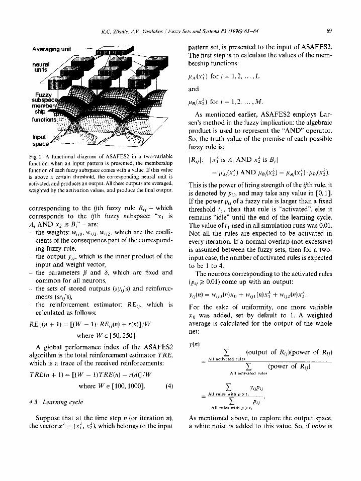
The estimation of Wo, wl, w2 in each subspace, is made with the aid of the ANASA II updating rule. The outputs produced from every neuron are combined to approximate the function f i n the whole of its domain. So each of the L x M subspaces is associated with one possible fuzzy rule and a neural unit, respectively (see Fig. 2).

4.2. Description of the variables used in ASAFES2

There are L × M neutral units, running separately. All the variables used by a single unit are used by ASAFES2 in this case as L × M matrices. The parameters and variables of the neural unit

K.C. Zikidis, A.V. Vasilakos / Fuzzy Sets and Systems 83 (1996) 63-84 69

Fig. 2. A functional diagram of ASAFES2 in a two-variable

function: when an input pattern is presented, the membership

function of each fuzzy subspace comes with a value. If this value is above a certain threshold, the corresponding neural unit is

activated, and produces an output. All these outputs are averaged,

weighted by the activation values, and produce the final output.

corresponding to the ijth fuzzy rule Ri~ which corresponds to the ijth fuzzy subspace: "X 1 is A~ AND x2 is Bf' - are: - the weights: W~jo, wij~, wij2, which are the coeffi-

cients of the consequence part of the corresponding fuzzy rule,

- the output y~, which is the inner product of the input and weight vector,

- the parameters fl and ~, which are fixed and common for all neurons,

- the sets of stored outputs (syifs) and reinforcements (stirs),

- t h e reinforcement estimator: REi~, which is calculated as follows:

REij(n + 1) = [(W - 1). RE~j(n) + r(n)]/W

where W e [50, 250].

A global performance index of the ASAFES2 algorithm is the total reinforcement estimator TRE, which is a trace of the received reinforcements:

TRE(n + 1) = [(W -- 1)TRE(n) + r(n)]/W

where W e [-100, 1000]. (4)

4.3. Learning cycle

Suppose that at the time step n (or iteration n), the vector x ~ = (x~, XzZ), which belongs to the input

pattern set, is presented to the input of ASAFES2. The first step is to calculate the values of the membership functions:

~A,(X~') for i -- 1,2 . . . . . L

and

pB,(x~t for i = 1,2 . . . . . M.

As mentioned earlier, ASAFES2 employs Lar- sen's method in the fuzzy implication: the algebraic product is used to represent the "AND" operator. So, the truth value of the premise of each possible fuzzy rule is:

IRi~l: Ix~ is Ai AND x2 ~ is Bj[

X 2 X 2 =/~A,(X~) AND #sj(x~) = PA,( 1)'~B,(2).

This is the power of firing strength of the/j th rule, it is denoted by p~j, and may take any value in [0, 1]. If the power p~j of a fuzzy rule is larger than a fixed threshold tl, then that rule is "activated", else it remains "idle" until the end of the learning cycle. The value of tl used in all simulation runs was 0.01. Not all the rules are expected to be activated in every iteration. If a normal overlap (not excessive) is assumed between the fuzzy sets, then for a two- input case, the number of activated rules is expected to be 1 to 4.

The neurons corresponding to the activated rules (Pij >~ 0.01) come up with an output:

y~An) = W~jo(n)xo + wij~(n)x~ + w~j2(n)x~.

For the sake of uniformity, one more variable x0 was added, set by default to 1. A weighted average is calculated for the output of the whole net:

y(n) (output of Rij)(power of Rij)

~--- All activated rules

(power of Rij) All activated rules

YijPij All rules with p ~> t I

2 Pij All rules with p/> t t

As mentioned above, to explore the output space, a white noise is added to this value. So, if noise is

70 K.C. Zikidis, A.V. Vasilakos / Fuz~ Sets and Systems 83 (1996) 63-84

a value taken from a standard Gaussian distribution N[0, 1], with mean 0 and standard deviation 1, the output value of the net is

output(n) = y(n) + a(n)noise

where a(n) = a l l - TRE(n)].

The output is properly scaled, according to the problem, and is offered to the environment, which evaluates it and returns a reinforcement signal r(n). In the general case, r is a random variable, R(x,y) , with probability distribution function P[R(x , y) <~ r] and its expected value shows how good was the output y, for the given input pattern X 2"

The neural units of the activated fuzzy rules receive this reinforcement and proceed to the updating of their weights, as described in the previous section. After the weight updating, they store the output y~j(n) and reinforcement r(n) in the place of the old output sy~ and reinforcement sr~, regis- tered the last time the same input pattern was presented. Finally, they update their reinforcement estimators.

This was the description of a complete learning cycle, for the case of a two-variable function or a system with two inputs and one output. Gener- ally, the dimension of the matrices is equal to the number of inputs. On the other hand, if a multi- output model is considered, then the number of separate ASAFES2 schemes required will be equal to the number of outputs.

4.4. Some notes and discussion

To reduce computational burden and memory requirements, a second threshold t2 is introduced, which determines when a neural unit should update and when it should not. In most simulation runs t2 was set to 0.5. In this way, if the power p~j of the rule R~j, is above tx but below t2, then the corresponding unit simply produces an output but does not make any kind of updating (weights or memory). If pij is above t 2 then the unit produces an output and carries on the updating procedure. In this way, multiple registrations of input patterns which may belong to more than one fuzzy sets are limited.

The firing strength Pij determines how much the fuzzy rule Rij affects the output. Therefore, it should also determine how much the rule Rij changes. This observation leads to the introduction of one more coefficient in the weight updating equation (1): p~j. In this way, the weight updating of the ijth neural unit is made according to the following equation:

w~jk(n + 1)

= Wjk(n) + pij[3 [ 1.1 -- RE(n)] ]drij(n)]F [drii(n)] Xk(n)

+ 6 dWi~k(n) for k = 0, 1, 2. (5)

The same applies to the calculation of RE~(n) of the /jth neuron, which becomes

REij(n + 1) = E(W - pij)REij(n) + piT(n)]/W,

W > 0. (6)

Considerable effort has been made in the design of the algorithm to reduce the need for memory stor- age and computational power. Of course, the matrices with the stored reinforcements and output values cannot be characterized negligible, but this is the price we have to pay when speed is an essential factor and the available information is not "instructive" but "evaluative". Each neuron has to keep records of previous actions (sy~)) and reinforcements (sr~) to make comparisons and decide about the updating. This algorithm was designed for use as software in a serial, digital computer. The fact that a number of separate units are running together should not be disappointing, because, in every iteration, only the units corresponding to activated rules (p~j/> tl) take part in the output calculation, and from these units, only the "considerably activated" (p~ ~> t2) update their regis- ters. For example, even if5 x 5 x 5 = 125 units were required to approximate adequately a 3-input function, only a maximum of 8 units could be activated at the same time. However, a special hardware implementation would naturally increase the speed considerably.

As mentioned in the beginning of this section ASAFES2 performs parameter identification and assumes that structure identification is already made. However, it helps in some ways in structure identification:

K.C Zikidis, A. IL Vasilakos /Fuzzy Sets and Systems 83 (1996) 63 84 71

First, the number of the fuzzy rules required is much less than the number required by the classical fuzzy reasoning method. In other words, while the min-max-centroidal method needs 5 or 7 or 9 fuzzy sets in each dimension, ASAFES2 (which employs the Sugeno fuzzy reasoning method) can reach a better performance index using fewer fuzzy sets. Second, the premise parameter identification is not very critical, since the weights in the consequence part can compensate (up to a limit) for the choice of not optimal premise parameters. Third, the use of a separate performance index, REij, for each fuzzy subspace enables the discovery of "problematic" regions in the input space. This, if a certain RE is lower than the neighbouring ones, then the function cannot be approximated adequately in this fuzzy subspace, and further segmentation should be considered, for this supspace at least. Furthermore, ASAFES2 helps in selecting the input variables from the input candidates: first, all candidates are employed and then, if relatively very small coefficients (weights) are assigned to one of them this candidate does not possibly affect the output and can be totally eliminated. Then, the sets of consequence relations corresponding to every fuzzy set of this variable are compared. If they are found similar, that candidate is excluded. Concluding, speed and ease of use of ASAFES2 allow identification using trial and error.

5. Delayed reinforcement and ASAFES2 in the adaptive heuristic critic

Associative reinforcement learning was introduced by Barto and colleagues [1-3], as an approximation method combining optimization under uncertainty, learning automata and supervised classification. It provides the theoretical and practical background for approaching problems difficult to solve with supervised learning, e.g., tasks where information is poor, noisy, and is available on the way or delayed (not a priori) [3, 4, 12, 14].

In the last case, where the reinforcement signal comes after a series of actions, the kind of algorithms as ANASA II (which require the reinforcement signal to evaluate the last action taken) would perform very poorly. To deal with delayed or generally poor

quality reinforcement tasks, the Temporal Differ- ence Methods were introduced [23], where an evaluation function characterizes the different states. Updating is made whenever there is a change in the evaluation function, i.e. whenever the system under control moves to a state with different evaluation than the previous one. To estimate the evaluation function an auxiliary neural network was used [3]. This net was the Adaptive Critic Element or simply critic. The critic receives system state information from the input vector, and predicts (in most cases) the infinite discounted cumulative outcomes:

~ 7kr(n+k), 7~[0,1). k=O

This is a natural quality measure of each state, containing time information, and implies that reinforcements coming within the immediately following time steps "count" more in the evaluation of this state than reinforcements which will come later on. 7 is the discount rate parameter, which controls the extent to which a reinforcement would affect the evaluation as a function of the reception time. If r(n + 1) is the reinforcement received after execut- ing an action at time step n, then the evaluation function of state x(n) = x is

J(x)=~I~=oTkr(n+l+k)'x(n)=xl'k

where ~ [ ] is the expectation operator, with re- spect to the action taking policy of the learning scheme. Suppose that the system is in state x and p(n) is the estimation of J(x). After the execution of an action, the system will enter state y where the estimation of J(y) is p(n + 1). p(n), trying to learn to estimate J(x) as described in the previous equation, has to predict:

g[r(n+ 1)+ k=l~ 7kr(n+l +k)[x(n+ 1 ) = y 1

= r(n + 1)

+g 7k+lr(n +1 + k + 1)[x(n +1) = y k

=r(n +1) + 7 ' N 7kr(n +2 +k)lx(n+l) =y I_k=O

-- r(n + 1) + ,/.J(y).

72 K.C. Zikidis, A.V. Vasilakos / Fuzzy Sets and Systems 83 (1996) 63 84

Namely, in every time step p(n) tries to predict r(n + 1) + 7 "p(n + 1). Therefore, the learning error is

error(n) = r(n + 1) + 7 . p(n + 1 ) - p(n)

ASAFES2 can be used to learn the evaluation function. The learning rule is

w(n + 1) = w(n) + p'fl 'error(n)'x(n) + ~dw(n). (7)

On the other hand, the controller network (actor) receives the input pattern and comes up with an output (the action to be taken). A noise, which is a quite essential element in reinforcement learning theory, is added, resulting in a perturbation of the actual output and a possible difference in the expected evaluation value, which, in turn, results in learning. Noise is a way of exploring the action space, searching for the direction of higher reinforcement. If a(n) is the standard deviation of noise, output(n) is the actual output and y(n) the output without noise, then the quantity corresponding to the "learning error" in time step n is

output(n) - y(n) [r(n + 1) + 7"p(n + 1 ) - p(n)]

o'(n)

The term ( o u t p u t - y ) / a is the normalized perturbation [11, 12], and if there are no limits for output, it is actually the noise added to y. The underlying idea of the equation above is that if the "actual" outcome r(n + 1) + 7"p(n + 1) is better than what was expected, i.e p(n), then the change should be proportional to and in the same direction as the noise, which is supposed to have caused this difference. Otherwise, the change should be to the opposite direction. If an ASAFES2 scheme was used as the actor network, the learning rule would be

w(n + 1) = w(n) + p'f l error(n)

output(n) × - y(n) x(n) + a dw(n). (8)

~(n)

In the simulation section, the cart-pole stabilization problem will be solved with a configuration like the one described above, where the ASAFES2 architecture is used both for the actor and the critic net. The steps of an actor-crit ic configuration algorithm, based on ASAFES2, in a few words, are:

1. Initialize weights in both actor and critic net, setting them to zero.

2. Present input pattern (state vector) to both nets.

3. Calculate output of critic ASAFES2 (estimated evaluation of current state): p(n).

4. Calculate output of actor ASAFES2 (expected action): y(n).

5. Add a noise with zero mean and standard deviation a(n) to y(n).

6. Scale and limit properly the obtained value, according to the specific problem.

7. Apply control action according to the actual output value calculated in Step 6.

8. Receive reinforcement r(n + 1). 9. Obtain the new state vector (input variables

normalized in [ - 1, + 1]. 10. Calculate new membership function values. 11. Calculate new output of critic net (estimated

evaluation of this state): p(n + 1). 12. Calculate learning error: error(n) = r(n + 1)

+ 7"p(n + 1) - p(n). 13. Update actor and critic network weights,

according to (7) and (8), with the old state vector and membership function values.

14. With the new state vector and membership function values, go to step 2.

6. Simulation

In this section, the shape of the membership function curves will be discussed in detail and then some illustrative examples will be presented: a static function approximation, using noise-free and noisy information; the modelling of the Box-Jenkins gas furnace, and the cart-pole stabilization task. All runs were made on a 486/80 MHz PC in C + +.

6.1. The double logistic membership function

The particular membership function used in the simulation was neither triangular, nor trapezoidal. It was a double logistic function: two symmetric logistic functions concatenated (see Fig. 3). The resulting function has a smooth, bell-shaped curve, and can be safely considered as convex. Compared

K.C. Zikidis, A.V. Vasilakos / Fuzzy Sets and Systems 83 (1996) 63-84 73

slope at I c-l.zs.h , , , , ~

!

/ o / c-1.75.h c

Fig. 3. The double logistic function.

\ threshok \

t c+1.75.h

to the Gaussian function, it is r~ore "flexible", offer- ing more parameters to tune, with the same computational cost. It seems similar to the /7 function curve [-36]. The authors found this function efficient and easy to handle.

The subroutine, which was used to divide an interval [LO, HI], LO, HI e 9~ into L fuzzy sets A~, i = 1, . . . , L, is depicted in the following lines:

Let h = (HI - LO)/(L - 1). This gives the length of the (L - 1) intervals, in which the initial interval is divided, by the centres of the L fuzzy sets. So, the centre c~ of the fuzzy set A1 is in LO, the centre c 2 of A 2 is in LO + h, the centre c3 of A3 is in LO + 2h, etc. The points where I~A,(x)= 0.5 are: c ~ - 1.75h and ci + 1.75h. The coefficient of h is a parameter that affects the overlap. The value 1.75 was found adequate in most cases. Now we can define the membership function of the fuzzy set A~ with centre ci:

1 if x >~ ci,

1 + exp{sl[x - (ci + 1.75h)]}

1 if x < c~.

1 + exp{ - sl[x - (ci - 1.75h)]} (9)

sl determines the slope of the logistic functions at the points ci - 1.75h and ci + 1.75h. It is calculated as a function of h, as follows:

s l = d / h , w i t h 5 ~ d ~ 15.

The membership curves of the fuzzy sets, into which the input variable ranges are divided, do not have to be similar. However, in the simulation of the algorithm, the parameter d and the coefficient of h were common for all membership functions employed in an input space partitioning. It should also be noted that ]~A,(X) n e v e r reaches 1 or 0. That is why the threshold t~ was set to 0.01 (and not to 0).

6.2. First example

The first example is the approximation of a non- linear, static function with two input variables (see Fig. 4(a)):

f ( x 1, x2 ) = - 90' exp( - 0.0002 x 2) sin(Tr x 1/90),

with domain - l l 0 < x a < + l l 0 a n d - 120< x 2 < +120, and range - 9 0 < f ( x a , x 2 ) < +90 . The function was learned through a set of 100 input patterns, which were randomly selected but repre- sented the function adequately. These input patterns were presented with a random order to the algorithm, not sequentially. To restrict the reinforcement in [0, 1], for the input pattern x ~ = (x~, x2~), the following function was used:

r (n )= exp [ - f ( x ~ ' x ~ ) - Y ( n ) 1 1 - 8 - 0 - (10)

i.e.

desired o u t p u t - actual output r, ,exp( ut ar ab e an ) (11)

Of course, in a single-output case like this, the reinforcement given in (11) is a measure of the learning error, and we cannot claim that the information is simply evaluative. However, still ASAFES2 receives less information, since it is a function of the absolute value of the error.

Each variable range was divided into 3 fuzzy sets, with membership functions defined in (9), where d = 10. If AI, A2, A3, are the 3 fuzzy sets dividing the range of variable x~, then h = 110, and ci = - 110 + (i - 1)h, i = 1, 2, 3. In the same way, the range of the variables x2 is divided into the fuzzy sets BI, B2, B3. The values of the thresholds were t~ = 0.01, t2 = 0.5. The value of W of Eq. (4)

74 K.C. Zikidis, A.V. Vasilakos /Fuzm, Sets and Systems 83 (1996) 63-84

100 --

80- -

60 - -

40- -

20 - -

0 - -

-20 --

-40--

-60 --

- 8 0 -

-1 O0 ~ o

(a)

100--

80--

60- -

40 - -

20 - -

0 - -

-20- -

-40- -

-60- -

- 8 0 -

-100- ~ ~ - - - - - - ~ 7 - ~ ~ ~

(b) Fig. 4. (a) The original funct ion surface. (b) The funct ion learned at TRE = 0.9.

K.C. Zikidis, A.K Vasilakos / Fuzzy Sets and Systems 83 (1996) 63 84 75

100 - -

8 0

6 0

40

-40

-8o ~

100

' ~

,oo~ ~ 8O

60

40

-20

-40

-ii

-100

(c)

Id) ~ x Fig. 4. (c) The function learned at T R E = 0.95. (d) The function learned at T R E = 0.98.

76 K.C. ZiMdis, A.K Vasilakos / Fuzzy Sets and Systems 83 (1996) 63 84

Table 1 Funct ion approximat ion compar i son results: ASAFES2 and back-propagat ion

ASAFES2 trained by ANASA II Trained by LMS B A C K - P R O P

Average Average Average Task: i terations/ Parameter i terations/ Parameter iterations/ Parameter function Successful average values average values Successful average values f (x~ ,x: ) runs time (in s) used time (in s) used runs time (in s) used

No noise 100% 2979/0.6 ~ = 0.75 2074/0.34 fl = 0.5 13 = 0.25 6 = 0 ,5 = 0.9

Noise 1% 100% 3300/0.74 x = 1.0 2146/0.39 fl = 0.4 /~ = o.3 ~ = o

6 = 0.9

Noise 10% 100% 28455/6.26 c~ = 1.25 5156/0.98 fl = 0.04 fl = 0.016 fi = 0.5 ~ = 0.975

85% 22 769/7.88 q = 0 . 7 a = 0.9

96% 31 810/10.13 r / = 0.6 a = 0.9

60% 46400./28.7 See text

was set to 500. Initially the weights are set to zero. All parameters affecting the fuzzy partition can be altered on line, enabling location of the optimal values. Especially, the centres (cl, c2, c3), d (it is reminded that sl = d/h), and the coefficient of h (which was set to 1.75) if changed on the way, result in different fuzzy sets of the input variables and thus affect the overall performance.

ASAFES2 showed a very smooth performance, converged very fast until T R E = 0.98 and then fine tuned to reach T R E > 0.99. In Fig. 4(a) is the graph of the original function. In Figs. 4(b)-(d), there are three consecutive learning phases of a single run of the algorithm, at T R E = 0.9, 0.95 and 0.98, respectively.

ASAFES2 was also trained with noisy information. White noise is added to the feedback:

r, t (n) = r(n) + 0.01-noise,

where noise has a standard Gaussian distribution (mean 0, standard deviation 1). In this way, the feedback is corrupted with 1% noise. A "worse" feedback, corrupted with 10% noise was also used. It was obtained from the above equation, except for the coefficient of noise, which was 0.1. However, T R E was evaluated directly from the noise-free reinforcement, giving a more accurate performance measure. The noisy reinforcement was used only in the updating procedure, to deteriorate learning.

1.00

095

0.90

1

iterations x 1000 12 24 3.6 4.8 6.0 7.2 8 4 96 11.8 12

TRE (Total Reinforcement Estimator.)

Fig. 5. Plot of TRE (Total Reinforcement Estimator) over time, for ten individual runs of ASAFES2 for the first learning task.

Results are shown in Table 1. As a stopping criterion the inequality T R E > 0.98 was used. In Fig. 5 are the plots of T R E ' s of 10 individual runs, as functions of time, for the noise-free case. It should be pointed out that ASAFES2 always learned the function, unless the learning rate was quite high and one or more neurons were driven into saturation (the weights reached very high values and learning was disabled).

The values of ~, [3, and 6 generally depend on the task. A large value for the parameter ~ gives too much exploration, and, although it initially gives a fast convergence rate, it prevents the algorithm

K.C. Zikidis, A.K Vasilakos / Fuzzy Sets and Systems 83 (1996) 63 84 77

from reaching a very high TRE. A small value for leads to slow convergence. On the other hand,/3 is

a very critical parameter, because if it takes a large value, will probably lead the weights to saturation and stop learning completely. 6 usually takes a high value: 0.5 to 0.975.

Even though our primary intention was to explore the behaviour of ASAFES2 trained by reinforcement learning, for reasons of completeness, it was also trained by a supervised algorithm, the well-known LMS. In this case, the learning rule is:

1.00

0,9. ~

1 PI

i terat ions x 1 0 0 0 - - - 6 12 18 24 30 36 42 48 54 60

" i ' i ~ ' ~ . . . . . . i ~

;)? , i " ~" : '

' P e r f o r m a n c e I n d e x . )

w(n + 1)

= w(n) + pfl [normalised error (n)]x(n) + 6 dw(n),

Fig. 6. Plot of PI (Performance Index) over time, for ten individual runs of back-propagation for the first learning task.

where the error is normalised in [ - 1, 1]. The re- suits are shown in Table 1.

Multi-layer perceptron topologies, with two input units, one output unit, and one or two hidden layers with up to 30 units, were also trained, with the back-propagation algorithm (generalized delta rule [19]), from the same 100 examples. Several combinations of values for the parameters (learning rate and momentum term coefficient) were used, to achieve the best results.

The back-propagation algorithm was found to be slower, and unreliable in many cases. The time needed (both in terms of real time and number of iterations) was greater than the time ASAFES2 needed to reach the same stopping criterion. Many times it got "stuck" unable to learn the function properly. The best performance was achieved with one hidden layer with 8 or 10 units, learning rate 0.7 and momentum coefficient 0.9. The convergence rate was not stable, and was slower than ASAFES2, on the average. Larger networks converged in a more "smooth" way, but they were really slow. In Fig. 6 are the plots of the performance indices for ten individual runs as functions of time, for the noise-free case.

The input patterns were also presented randomly and the initial weight values were in [ - 0 . 5 , 0.5]. A relation similar to (11) was used to give a "reinforcement", in order to use Eq. (4) with W = 500 to obtain a reliable performance index PI, equivalent to TRE. The back-prop networks were trained with simulated noisy data, as well. A zero-mean Gaus- sian noise was added everytime to the learning

error. The standard deviation was again 1% of the output range in one case and 10% in the other. The learning rate ~/ and the momentum coefficient a could not remain constant and had to be sub- stituted with appropriate functions in the 10% noise case, or else back-prop could not learn beyond a limit. These functions were heuristically found and allowed the algorithm to reach PI > 0.98:

q = min(0.7, 1.1 - PI 6)

and

a = rain(0.9, 1.3 - pI6).

Results are also shown in Table 1. Generalized Radial Basis Function Networks

(GRBFNs) [9, 13] are a class of fast learning neural networks. In GRBFN the input space is trans- formed non-linearly into a high-dimensional space, where the task of classification or function approximation is more likely to be linearly solved. They are three-layer networks, with non-linear hidden units and a linear output unit. They have many similari- ties with the Sugeno fuzzy reasoning method, which reduces to the GRBFN if Gaussian membership functions are used and the consequence of a fuzzy rule is a single number and not a linear input- output relation. The functions most commonly used in the hidden layer are Gaussian functions of the form:

~pi(x) = exp I1 x - xc, II 2 width > 0

78 K.C Zikidis, A. td Vasilakos / Fuzz), Sets" and ,~vstems 83 (1996) 63 84

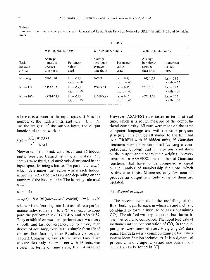
Table 2 Function approximation comparison results: Generalized Radial Basis Function Networks (GRBFNs) with 16, 25 and 36 hidden units

G R B F N

W i t h 16 h i d d e n u n i t s W i t h 25 h i d d e n un i t s W i t h 36 h i d d e n u n i t s

Average Average Average Task: iterations." Parameter i t e ra t ions / ' Parameter iterations/ Parameter function average values average values average values

,/'(XI, A72} time (in s) used time (in s) used time (in s) used

N o n o i s e 5880/1.91 l.r. = 0.95 2608 /1 .4 1.r. = 0.95 1945/1.35 1.r. = 0.95

w i d t h = 50 w i d t h - 45 w i d t h - 35

N o i s e 1 % 6522/2 .17 l.r. = 0.85 2788/1 .57 l.r. = 0.85 2010/1 .4 l.r. - 0.85

w i d t h = 50 w i d t h = 45 w i d t h = 35

N o i s e 1 0 % 45 714/15.41 l.r. = 0.15 15760 /8 .88 l.r. = 0.15 4670 /3 .68 l.r. - 0.15

w i d t h - 50 w i d t h - 45 w i d t h = 35

where ci is a point in the input space. If N is the number of the hidden units, and wi, i = l . . . . . N, are the weights of the output layer, the output function of the network is

f ( x ) - - 2iN- 1 Wi~Oi(X)

Networks of this kind, with 16.25 and 36 hidden units, were also trained with the same data. The centres were fixed, and uniformly distributed in the input space, forming a lattice. The parameter width ,

which determines the region where each hidden neuron is "activated", was chosen depending on the number of the hidden units. The learning rule used was:

w~(n + 1)

= wi(n) + lr ~pi (x)[normal ised error(n)] , i = 1 . . . . . N,

where lr is the learning rate. Just as before, a performance index equivalent to T R E was used, to com- pare the performance of G R B F N and ASAFES2. They exhibited an excellent performance, with very smooth and fast convergence, up to a very high degree of accuracy, even in this simple form (fixed centres, fixed learning rate). Results are shown in Table 2. Compar ing results from Tables 1 and 2, we can see that only the small net with 16 units was slower, in terms of time steps, than ASAFES2,

However, ASAFES2 runs faster in terms of real time, which is a rough measure of the computational complexity. All runs were made on the same computer , language, and with the same program structure. This can be attr ibuted to the fact that in a G R B F N with N hidden units, N Gaussian functions have to be computed (causing a com- putat ional burden) and all neurons contribute to the output and update their weights, in every iteration. In ASAFES2, the number of Gaussian functions that have to be computed is equal to the number of membership functions, which in this case is six. Moreover , only few neurons produce an output and only some of them are updated.

6.3. S e c o n d e x a m p l e

The second example is the modelling of the Box-Jenkins gas furnace, in which air and methane combined to form a mixture of gases containing CO2. The air feed was kept constant but the methane flow could be controlled. The input feed rate of methane and the concentra t ion of CO2 in the output gases were sampled every 9 s, giving 296 data pairs. This data set is a c o m m o n example for testing system identification techniques. It is a dynamical process with one input x (n ) and one output y(n).

The data can be found in [6].

K.C Zikidis, A. ~ Vasilakos /Fuzzv Sets and Systems 83 (1996) 63-84 79

To m a k e compar i sons with previous approaches , instead of T R E , ano ther per formance index will be employed here, the wel l -known mean square error:

(actual o u t p u t - model output ) 2 P I

,=IZ" (~umb~r ~(tr~llnT~ng e x ~ "

Previous approaches were made by Tong [26], Pedrycz [18], Xu [33], Takagi and Sugeno, and Sugeno and Yasukawa (posi t ion-gradient model) [22]. The best (lowest) P I achieved was 0.068 by the model of Takagi and Sugeno. Tha t model used only 2 rules with inputs:

y(n - 1), y(n - 2), y(n - 3), x (n - 1), x(n - 2), x (n - 3).

The p roposed scheme, t rained by ANASA II and using the same inputs, achieved a mean square error near 0.064 (after an extended run); the best per formance repor ted up to now. The two rules that comprise the model are:

R1: If y(n - 1) is L O W then y(n)

= 0.899y(n - 1) - 0.306y(n - 2) + 0.053y(n - 3)

- 0.01x(n - 1} + 0.013x(n - 2)

- 0.225x(n - 3) - 0.095.

R2: I f y ( n - 1) is H I G H then y(n)

= 1.442y(n - 1) - 0.528y(n - 2) - 0.086y(n - 3)

+ 0.047x(n - 1) - 0.122x(n - 2)

+ 0.032x(n - 3) + 0.066.

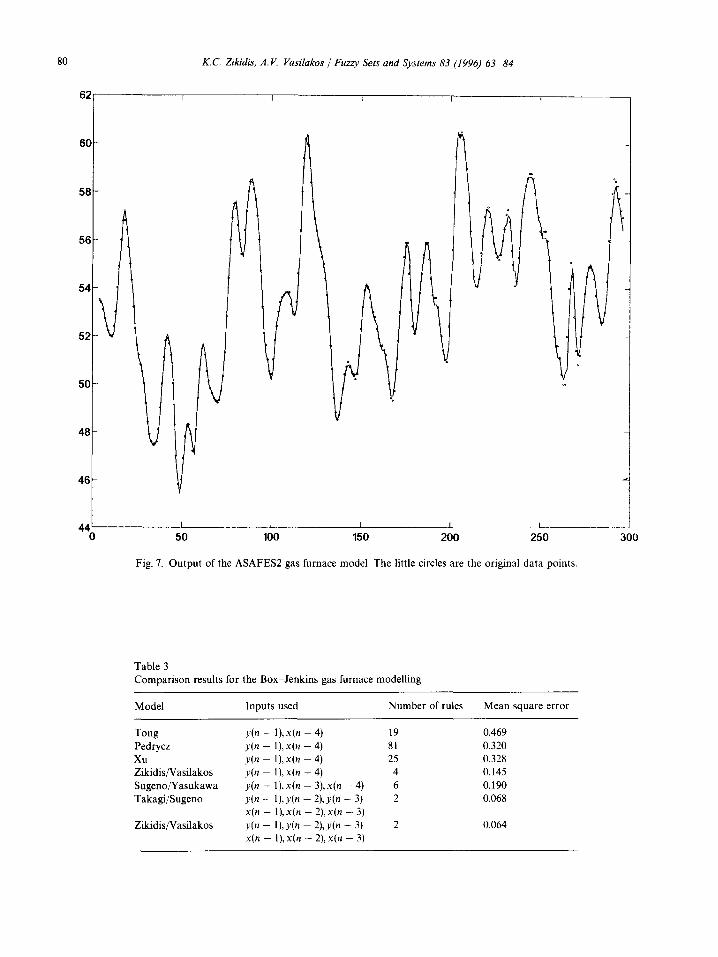
The membersh ip functions for L O W and H 1 G H are defined with the use of double logistic function presented earlier, considering that the range of y(n) is [49, 59] and d = 8. In Fig. 7 is the model output , where the little circles are the real gas furnace data.

Using these input variables, ASAFES2 reached a P I below 0.2 in 3318 iterations/0.45 s on average (e = 0.5,/~ = 0.75, (~ = 0.8). However, using y(n - 1), x(n - 4) as inputs (as in the first 3 approachest , it achieved a P I lower than 0.2 with only 4 rules in less than 2973 i terat ions/0.6s on the average (d = 8, :~ = 0.75,/~ = 0.25, 6 = 0.9). Compar i son results with previous approaches are shown in Table 3.

6.4. Third example

In the third example, an actor critic scheme, like that described in the previous section, with ASAFES2 used for both the actor and the critic, will balance the inverted pendulum. In this task, the control a lgor i thm has to learn to balance an upright pole (see Fig. 8), whose bo t tom is a t tached by a pivot to a cart, moving on a finite t rack in one dimension, by exerting right or left forces of limited magnitude. Movemen t of both cart and pole are allowed only in the vertical plane. The variables describing the state of the system, which will be the input variables to the controll ing a lgor i thm are: • 0 the angle of pole from the upright position

(degrees), • 0 the angular velocity of pole (degree/s), • x the horizontal posit ion of the cart 's centre (m), • "~? the velocity of cart (m/s). The only control action al lowed is a f o r c e r exerted on the cart (in N). The objective is to keep the pole as long as it is possible within the limits:

{ - 1 2 : ~ < 0 ~ < + 1 2 ~

2.4m ~< x ~< + 2.4m

using a force, whose magni tude satisfies - 10N ~<f~< + 10N. The equat ions of mot ion are ad-

opted f rom [14], including friction effects. The same model and parameters were used in [3]. Of course, the mot ion equat ions are assumed to be unknown to the controller. The parameters used are: gravity = 9.8 m/s 2, mass of pole and cart = 1.1 kg, mass of pole = 0.1 kg, half-pole length = 0.5 m, friction coefficient of the cart on the cart = 0.0005, friction coefficient of the pole on the cart = 0.000002. The equat ions of mot ion were simulated by the Eyler method, for a sampling interval of 0.02 s.

The controll ing a lgor i thm begins with naive knowledge, and makes some trials to learn to keep the pole up. A trial begins with the system in the initial state, in which all variables are zero, and ends when a failure occurs, that is x or 0 exceeded the limits. The reinforcement given to the a lgor i thm is

- 1 , if a failure has occurred, r ( n ) = 0, otherwise.

80

62

K . C . Z ik id i s , A . V . V a s i l a k o s / F u z z y S e t s a n d S y s t e m s 8 3 ( 1 9 9 6 ) 63 8 4

60

58

56

54

52

50

48!

46

44' 0

le

4

* °

I I I t I

50 100 150 200 250

Fig. 7. O u t p u t of the A S A F E S 2 gas furnace model. The little circles are the original da ta points.

300

Table 3 C o m p a r i s o n results for the B o x - J e n k i n s gas furnace model l ing

Model Inpu t s used N u m b e r of rules M e a n square error

T o n g y ( n - 1),x(n - 4) 19 0.469 Pedrycz y ( n - 1),x(n - 4) 81 0.320 Xu y ( n - 1),x(n - 4) 25 0.328 Zikidis /Vasi lakos y ( n - 1),x(n - 4) 4 0.145 S u g e n o / Y a s u k a w a y ( n - 1), x ( n - 3), x ( n - 4) 6 0.190 Takag i /Sugeno y ( n - 1), y ( n - 2), y ( n - 3) 2 0.068

x ( n - - l ) ,x(n - 2),x(n - 3) Zikidis /Vasi lakos y ( n - 1), y ( n - 2), y ( n - 3) 2 0.064

x ( n - l ) ,x(n - 2) ,x(n - 3)

I !

f3 ' f , . ) i i

! i

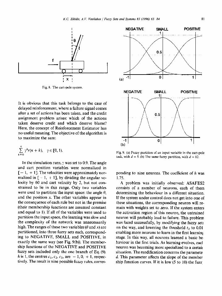
Fig. 8. The cart-pole system. NEGATIVE SMALL POSITIVE

It is obvious that this task belongs to the case of delayed reinforcement, where a failure signal comes after a set of actions has been taken, and the credit assignment problem arises: which of the actions taken deserve credit and which deserve blame? Here, the concept of Reinforcement Estimator has no useful meaning. The objective of the algorithm is to maximize the sum:

~, Tkr(n + k), 7~ [0, 1). k = O

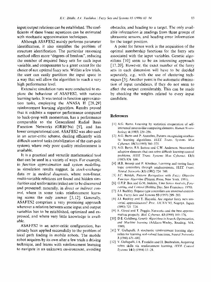
In the simulation runs, ? was set to 0.9. The angle and cart position variables were normalized in [ - 1, + 1]. The velocities were approximately normalized in [ - 1, + 1], by dividing the angular velocity by 60 and cart velocity by 2, but not con- strained to lie in this range. Only two variables were used to partition the input space: the angle 0, and the position x. The other variables appear in the consequence of each rule but not in the premise (their membership functions are assumed constant and equal to i). If all of the variables were used to partition the input space, the learning was slow and the complexity of the network was unnecessarily high. The ranges of these two variables (0 and x) are partitioned, into three fuzzy sets each, corresponding to NEGATIVE, SMALL and POSITIVE, in exactly the same way (see Fig. 9(b)). The membership functions of the NEGATIVE and POSITIVE fuzzy sets included only the one branch of Eq. (9). h is 1, the centres cl, c2, c3, are - 1, 0, + 1, respectively. The result is nine possible fuzzy rules, corres-

NEGATIVE SMALL POSITIVE

/x\ / \ / \

-1 0 1 (a)

m

K.C. Zikidis, A.F. Vasilakos / Fuzzy Sets and Systems 83 (1996) 63-84 81

-11 0 (b)

Fig. 9. (a) Fuzzy partition of an input variable in the cart-pole task, with d = 5. (b) The same fuzzy partition, with d = 12.

ponding to nine neurons. The coefficient of h was 1.75.

A problem was initially observed: ASAFES2 consists of a number of neurons, each of them determining the behaviour in a different situation. If the system under control does not get into one of these situations, the corresponding neuron will remain with weights set to zero. If the system enters the activation region of this neuron, the untrained neuron will probably lead to failure. This problem was faced successfully, by modifying the fuzzy set, on the way, and lowering the threshold t2 to 0.01 enabling more neurons to learn in the first learnin~ stage. In this way, all neurons learned a basic be haviour in the first trials. As learning evolves, eact neuron was becoming more specialized to a certail situation. The modification concerns the paramete d. This parameter affects the slope of the member ship function curves. If it is low (5 to 10) the fuzz

82 K.C. Zikidis. A. K Vasilakos / Fuzz), Sets and Systems 83 (1996) 63 84

IO000G

1 time steps

0 100 L ~u_t,I l,/x _

number of trials -~,

Fig. 10. Plot of 50 individual runs of ASAFES2 for the cart-pole problem: only 2 did not succeed in learning the task within the 100 trials. 35 out of 50 learned in 25 trials.

sets expand and appear more "fuzzy". In Fig. 9(a), is the fuzzy partition of a variable with d = 5. While it increases, the fuzziness is reduced. In Fig. 9(b) is the same partition with d = 12. So, d was replaced by d* (a function of the number of trials so far):

d* = d number of trials with d = 12. number of trials + 3

The inputs and the input partition were common to the two ASAFES2 nets, implementing the actor and the critic. The updating rule for the ASAFES2 used for the critic net, was Eq. (7), with [3 = 0.5 and b = 0. Eq.(8) was the updating rule for the ASAFES2 implementing the actor net, with fl = 0.075, 6 = 0.5, and a(n) was a function of the output of the critic net p(n):

a(n) = ~lp(n)l + 0.001 with ~ = 2.5.

This increases the stochastic search when p(n) is going to predict a failure, i.e. when it is near - 1. An important simplification allowed by the nature and the formulation of the task is the omission of the bias weights, in both nets. The learning error was [4]:

error(n) =

r(n + 1) - p(n) if failure has occurred,

r(n + l) + 7p(n + 1) - p(n), otherwise.

The algorithm was supposed to have learned when it exceeded 100 000 time steps, corresponding to more than half an hour of simulated time. In Fig. 10 there is a typical plot of the time steps until

failure for 50 different runs. A run is a set of trials, where the algorithm tries to learn to keep the cart- pole system balanced as long as possible (there is no exact success in finite time). A run is considered to be successful if the algorithm has learned the task in less than 100 trials. Almost all runs were successful, and in 35 runs the algorithm learned in less than 25 trials. Only 2 out of 50 runs were unsuccessful. If the runs appear to be less than 100, this is because many runs ended before the 25th trial and cannot be distinguished.

Tests to explore the robustness of the algorithm were also performed. A well-trained ASAFES2 was successfully used to balance cart-pole systems with different parameters than the ones mentioned above, without further training. In the first test, the mass of the pole was increased by 10 times. In the second test, the mass of the cart was increased by 10 times. The length of the pole was increased (doubled) and then shortened (by a factor of 5). In the last tests the length of the pole was shortened (by a factor of 5) and the pole weight was simulta- neously reduced by a factor of 10. Finally, the pole length was doubled and its weight was increased 10 times. In all these cases ASAFES2 could balance the system. The results obtained are better than the ones in [3], and comparable to these reported in [-4, 14].

7. Conclusion-future work

A new architecture for fuzzy computing was presented which exploits the advantages of fuzzy logic and especially the Sugeno's reasoning, and the learning ability of reinforcement neural algorithms. ASAFES2 is a novel, integrated approach to the function approximation task, being a simple and reliable algorithm with fast and smooth convergence, which can "discover" and learn a function by interacting with a noisy environment. Besides, it states the learned function in an understandable form: a set of fuzzy implications and linear relations. This is very important in a real application: it enables the incorporation of prior knowledge into an ASAFES2 net. Its learning capability and performance are based on the idea of segmenting the input space into smaller fuzzy parts; where linear

K.C Zikidis, A.V. Vasilakos / Fuzo' Sets and Systems 83 f1996) 63 84 83

input/output relations can be established. The coefficients of these linear equations can be estimated with stochastic approximation techniques.

Although ASAFES2 mainly performs parameter identification, it also simplifies the problem of structure identification. The particular reasoning method offers more "degrees of freedom", reducing the number of required fuzzy sets for each input variable, and compensates to a great extent for the choice of not optimal fuzzy sets. Within a few trials, the user can easily partition the input space in a way that will allow the algorithm to reach a very high performance level.

Extensive simulation runs were conducted to explore the behaviour of ASAFES2, with various learning tasks. It was tested in function approximation tasks, employing the ANASA II [28,29] reinforcement learning algorithm. Results proved that it exhibits a superior performance compared to back-prop with momentum, has a performance comparable to the Generalized Radial Basis Function Networks (GRBFNs) [9], and has lower computational cost. ASAFES2 was also used in an actor-critic scheme, dealing efficiently with difficult control tasks (stabilization of the cart-pole system), where only poor quality reinforcement is available.

It is a practical and versatile mathematical tool that can be used in a variety of ways. For example, in function approximation and system modelling, as simulation results suggest. In stock-exchange data or in medical diagnosis, where non-linear, multi-variable relations are found and hidden sim- ilarities and uniformities (rules) are to be discovered and presented; naturally, in direct or indirect control, where in some tasks reinforcement learning seems the only answer [3,12]. Generally, ASAFES2 comprises a very promising approach wherever a relation between some input and output variables has to be established, optimized and expressed, and where very little knowledge is available.

ASAFES2 in an actor-critic configuration, has already been applied successfully to the problem of local path finding in mobile robots. The mobile robot acquires by its own after a few trials a driving technique, and learns with reinforcement learning to navigate in an unknown environment, avoiding

obstacles, and heading to a target. The only available information is readings from three groups of ultrasonic sensors, and heading error information for the target position.

A point for future work is the acquisition of the optimal membership functions for the fuzzy sets associated with the input variables. Genetic algorithms [10] seem to be an interesting approach [17,20]. However, the exact number of the fuzzy sets in each dimension will have to be decided separately, e.g., with the use of clustering techniques [5]. Another point is the automatic elimina- tion of input candidates, if they do not seem to affect the output considerably. This can be made by checking the weights related to every input candidate.

References

[I] A.G. Barto, Learning by statistical cooperation of self- interested neuron-like computing elements. Human Neuro- biology 4 (1985) 229 256.

[2] A.G. Barto and P. Anandan, Pattern recognizing stochastic learning algorithms, IEEE Trans. Systems Man Cybernet. 15(3) (1985) 360-375.

[3] A.G. Barto, R.S, Sutton and C.W. Anderson, Neurontike adaptive elements that can solve difficult learning control problems, IEEE Trans. Systems Man Cybernet. 13(5) (1983) 834 846.

[4] H.R. Berenji and P. Khedkar, Learning and tuning fuzzy logic controllers through reinforcements, IEEE Trans. Neural Networks 3(5) (1992) 724-740.

[5] J.C. Bezdek, Pattern Recognition with Fuzzy Ol?jeeti~,e Function Algorithm (Plenum Press, New York, 1981).

[6] G.E.P. Box and G.M. Jenkins, Time Series Analysis, Fore- casting, and Control (Holden Day, San Francisco. 1970).

[7] J.J. Buckley, Sugeno type controllers are universal controllers, Fuzzy Sets and Systems 53 (1993) 299-303.

[8] J.J. Buckley and Y. Hayashi, Are regular fuzzy nets universal approximators? Proc. lJCNN'93, Nagoya, Japan (1993) 721 724.

[9] F. Girosi and T. Poggio, Networks and the best approximation property, Biol. Cybernet. 63 (1990) 169 176.

[ 10] D.E. Goldberg, Genetic Algorithms in Search, Optimization, and Maehine learning (Addison-Wesley, Reading, MA, 1989).

[11] V. Gullapalli, A stochastic reinforcement learning algorithm for learning real-valued functions, Neural Networks 3 (1990) 671 692.

[12] V. Gullapalli, J.A. Franklin and H. Benbrahim, Acquiring robot skills via reinforcement learning, IEEE Control Systems 14(1) (1994) 13 24.

84 K.C. Zikidis, A.I~ Vasilakos / Fuzzy Sets and Systems 83 (1996) 63-84

[13] S. Haykin, Neural Networks, a Comprehensive Foundation (Macmillan, New York, 1994).

[14] C.-T. Lin and C.S.G. Lee, Reinforcement structure/parameter learning for neural-network-based fuzzy logic con- t rol systems, IEEE Trans. Fuzzy Systems 2(1) (1994) 46-63.

[15] E.H. Mamdani and S. Assilian, Applications of fuzzy algorithms for control of simple dynamic plant, Proc. Inst. Elec. Eng. 121 (1974) 1585-1588.

[16] M. Mizumoto, Fuzzy controls under various fuzzy reasoning methods, Inform. Sci. 45 (1988) 129 151.

[17] D. Park, A. Kandel and G. Langholz, Genetic-based new fuzzy reasoning models with application to fuzzy control, IEEE Trans. Systems Man Cybernet. 24(1) (1994) 39-47.

[18] W. Pedrycz, An identification algorithm in fuzzy relational systems, Fuzzy Sets and Systems 13 (1984) 153 167.

[19] D. Rumelhart et al., Parallel distributed processing: explo- rations in the microstructure of cognition, Vol. 1 (MIT Press, Cambridge, MA, 1986).

[20] K. Shimojima, T. Fukuda and Y. Hasegawa, Self-tuning fuzzy modeling with adaptive membership function, rules, and hierarchical structure based on genetic algorithm, Fuzzy Sets and Systems 71 (1995) 295 309.

[21] M. Sugeno and G.T. Kang, Fuzzy modelling and control of a multilayer incinerator, Fuzzy Sets and Systems 18 (1986) 329-346.

[22] M. Sugeno and T. Yasukawa, A fuzzy-logic-based approach to qualitative modelling, IEEE Trans. Fuzzy Systems 1(1) (1993) 7 31.

[23] R.S. Sutton, Learning to predict by the methods of temporal differences, Machine Learning 3 (1988) 9 44.

[24] T. Takagi and M. Sugeno, Fuzzy identification of systems and its application to modelling and control, IEEE Trans. Systems Man Cybernet. 15 (1985) 116 132.

[25] K. Tanaka and M. Sugeno, Stability analysis and design of fuzzy control systems, Fuzzy Sets and Systems 45 (1992) 135-156.

[26] R.M. Tong, The evaluation of fuzzy models derived from experimental data, Fuzzy Sets and Systems 4 (1980) 1 12.

[27] S.G. Tzafestas, G.B. Stamou and K. Watanabe, Fuzzy reasoning through a general neural network model, in: S.G. Tzafestas and A.N. Venetsanopoulos, Ed., Fuzzy Reasoning in Information, Decision and Control Systems (Kluwer, Boston, 1994) 145 160.

[28] A.V. Vasilakos and N.H. Loukas, ANASA: a reinforcement learning algorithm in the field of real-valued neural computation, IEEE Trans. on Neural Networks, accepted.

[29] A.V. Vasilakos, N.H. Loukas and K.C. Zikidis, A.N.A.S.A. II: A novel, real-valued, reinforcement algorithm for neural unit/network, Proc. IJCNN'93 (Nagoya, Japan, 1993) 1417 1420.

[30] A.V. Vasilakos and G.I. Papadimitriou, A new approach to the design of reinforcement scheme for learning automata: stochastic estimator learning algorithms, Neurocom- puting 7 (1975) 275-297.

[31] A.V. Vasilakos and K.C. Zikidis, A.S.A.F.ES.: Adaptive Stochastic Algorithm for Fuzzy computing/function ES- timation, Proc. IEEE Internat. Conf. on Fuzzy Systems (FUZZ-IEEE'94) (Orlando, FL, 1994) 1087-1092.

[32] A.V. Vasilakos and K.C. Zikidis, A.S.A.F.ES.2: a novel, neuro-fuzzy architecture for fuzzy computing, based on functional reasoning, Proc. 4th IEEE Internat. Conf. on Fuzzy Systems FUZZ-IEEE/IFES'95, (Yokohama, Japan, 1995) 671-678.

[33] C.W. Xu and Z. Yong, Fuzzy model identification and self-learning for dynamic systems, IEEE Trans. Systems Man Cybernet. 17(4) (1987) 683-689.

[34] L.A. Zadeh, Fuzzy sets, Inform. and Control g (1965) 338-352.

[35] L.A. Zadeh, Outline of a new approach to the analysis of complex systems and decision processes, IEEE Trans. Systems Man Cybernet. 3 (1973) 28-44.

[36] L.A. Zadeh, A fuzzy-algorithmic approach to the defini- tion of complex or imprecise concepts, Internat. J. Man- Machine Studies g (1976) 249-291.

[37] H.-J. Zimmermann, Fuzzy Set Theory and Its Applications (Kluwer, Boston, 2nd rev. edn., 1991).

asafes2: a novel, neuro-fuzzy architecture for fuzzy computing, based on functional reasoning

Documents