arX

iv:a

stro

-ph/

0601

242v

1 1

1 Ja

n 20

06DRAFT VERSIONOCTOBER7, 2018Preprint typeset using LATEX style emulateapj v. 11/26/03

INTERSTELLAR PLASMA WEATHER EFFECTS IN LONG-TERM MULTI-FREQUENCYTIMING OF PULSAR B1937+21

R. RAMACHANDRAN , P. DEMOREST, D. C. BACKERDepartment of Astronomy and Radio Astronomy Laboratory, University of California, Berkeley, CA 94720-3411, USA;

e-mail: ramach, demorest, dbacker@astro.berkeley.edu

I. COGNARDLaboratoire de Physique et Chimie de l’Environnement, CNRS, 3A avenue de la Recherche Scientifique, F-45071 Orleans, France

A. L OMMENDepartment of Physics and Astronomy, Franklin and MarshallCollege, P.O.Box 3003, Lancaster, PA 17604, USA

Draft version October 7, 2018

ABSTRACTWe report here on variable propagation effects in over twenty years of multi-frequency timing analysis of pulsarPSR B1937+21 that determine small-scale properties of the intervening plasma as it drifts through the sightline. The phase structure function derived from the dispersion measure variations is in remarkable agreementwith that expected from the Kolmogorov spectrum, with a power law index of 3.66± 0.04, valid over aninferred scale range of 0.2—50 A.U. The observed flux variation time scale and the modulation index, alongwith their frequency dependence, are discrepant with the values expected from a Kolmogorov spectrum withinfinitismally small inner scale cutoff, suggesting a caustic-dominated regime of interstellar optics. This impliesan inner scale cutoff to the spectrum of∼ 1.3×109 meters. Our timing solutions indicate a transverse velocityof 9 km sec−1 with respect to the solar system barycenter, and 80 km sec−1 with respect to the pulsar’s LSR.We interpret the frequency dependent variations of DM as a result of the apparent angular broadening of thesource, which is a sensitive function of frequency (∝ ν−2.2). The error introduced by this in timing this pulsaris ∼2.2µs at 1 GHz. The timing error introduced by “image wandering” from the slow, nominally refractivescintillation effects is about 125 nanosec at 1 GHz. The error accumulated due to positional error (due to imagewandering) in solar system barycentric corrections is about 85 nanosec at 1 GHz.Subject headings:ISM: general — pulsars: general — radio continuum: general —scattering — turbulence

1. INTRODUCTION

The dispersion measure (DM) of a pulsar probes the col-umn density of free electrons along the line of sight (LOS).Observed DM variations over time scales of several weeksto years sample structures in the electron plasma over lengthscales of 1010 m to 1012 m. Diffraction of pulsar signals is theresult of scattering by structures on scales below the Fresnelradius, 108 m or so. The DM as well as the scattering mea-sure (SM) variability along the LOS to the Crab pulsar wasfirst reported by Rankin & Isaacman (1977), who reportedthat the DM variability poorly correlated with the SM vari-ability. Helfand et al. (1980) inferred an upper limit for DMvariations of a few parts in a thousand for several pulsars. Inan earlier study of PSR B1937+21 Cordes et al. (1990) mea-sured a DM change of∆DM ∼ 0.003 pc cm−3 over a periodof a thousand days. The work of Phillips & Wolszczan (1991)presented the variations of DM observed along the LOS toa few pulsars. They connected these variations to those ondiffractive scales, and derived an electron density fluctuationspectrum slope of 3.85±0.04 over a scale range of 107 − 1013

meters. Backer et al. (1993) report on further DM variabilityand show that the amplitude of the variations known at thattime are consistent with a scaling by the square root of DM.Another important investigation by Kaspi et al. (1994) stud-ied DM variations of the millisecond pulsars PSR B1937+21and B1855+09 over a time interval of calendar years 1984to 1993. In addition to establishing a secular variation in DMover this time interval, they also show that the underlying den-

FIG. 1.— Summary of our data sample. See text for details.

sity power spectrum has an index of 3.874±0.011, which isclose to what we would expect if the density fluctuations aredescribed by Kolmogorov spectrum. An anomalous disper-sion event towards the Crab pulsar was reported by Backer etal. (2000), where they report a DM “jump” as large as 0.1 pccm−3.

2 R. Ramachandran et al.

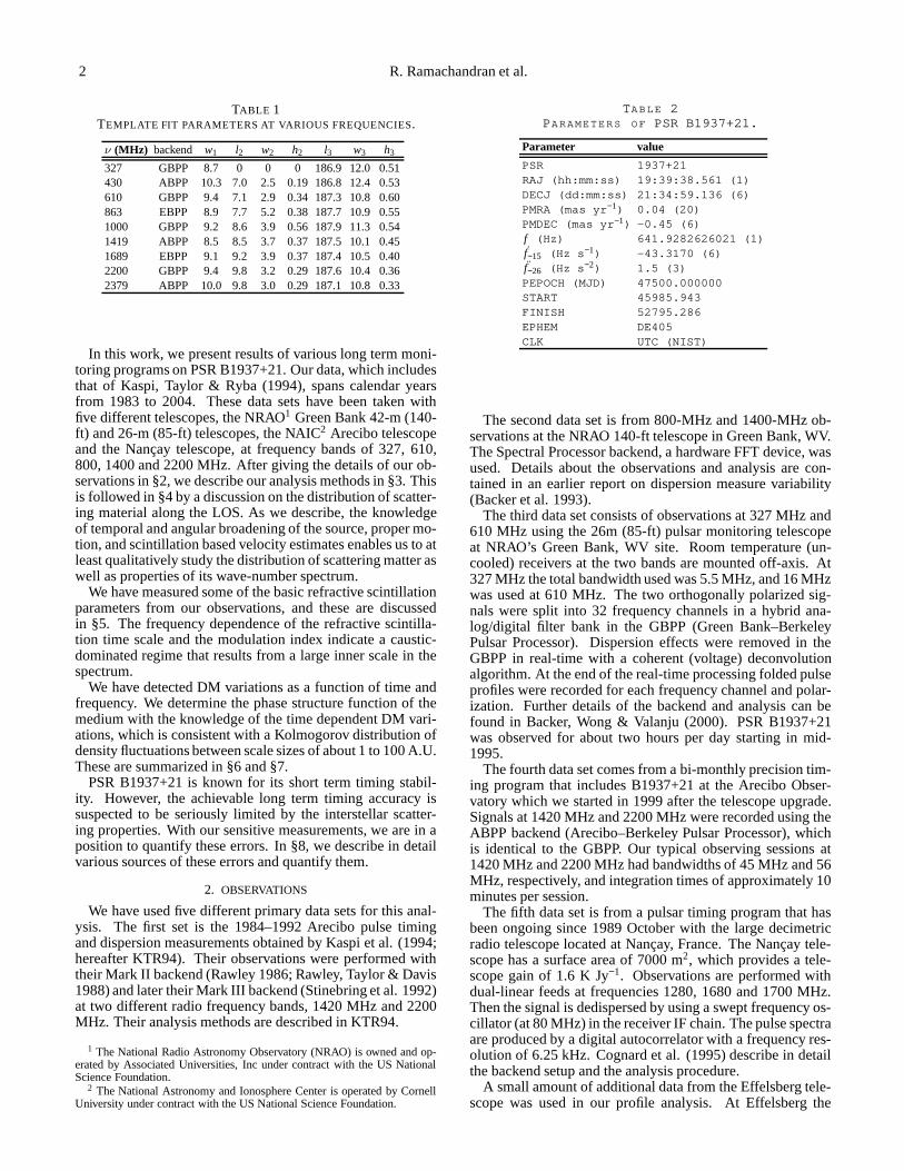
TABLE 1TEMPLATE FIT PARAMETERS AT VARIOUS FREQUENCIES.

ν (MHz) backend w1 l2 w2 h2 l3 w3 h3

327 GBPP 8.7 0 0 0 186.9 12.0 0.51430 ABPP 10.3 7.0 2.5 0.19 186.8 12.4 0.53610 GBPP 9.4 7.1 2.9 0.34 187.3 10.8 0.60863 EBPP 8.9 7.7 5.2 0.38 187.7 10.9 0.551000 GBPP 9.2 8.6 3.9 0.56 187.9 11.3 0.541419 ABPP 8.5 8.5 3.7 0.37 187.5 10.1 0.451689 EBPP 9.1 9.2 3.9 0.37 187.4 10.5 0.402200 GBPP 9.4 9.8 3.2 0.29 187.6 10.4 0.362379 ABPP 10.0 9.8 3.0 0.29 187.1 10.8 0.33

In this work, we present results of various long term moni-toring programs on PSR B1937+21. Our data, which includesthat of Kaspi, Taylor & Ryba (1994), spans calendar yearsfrom 1983 to 2004. These data sets have been taken withfive different telescopes, the NRAO1 Green Bank 42-m (140-ft) and 26-m (85-ft) telescopes, the NAIC2 Arecibo telescopeand the Nançay telescope, at frequency bands of 327, 610,800, 1400 and 2200 MHz. After giving the details of our ob-servations in §2, we describe our analysis methods in §3. Thisis followed in §4 by a discussion on the distribution of scatter-ing material along the LOS. As we describe, the knowledgeof temporal and angular broadening of the source, proper mo-tion, and scintillation based velocity estimates enables us to atleast qualitatively study the distribution of scattering matter aswell as properties of its wave-number spectrum.

We have measured some of the basic refractive scintillationparameters from our observations, and these are discussedin §5. The frequency dependence of the refractive scintilla-tion time scale and the modulation index indicate a caustic-dominated regime that results from a large inner scale in thespectrum.

We have detected DM variations as a function of time andfrequency. We determine the phase structure function of themedium with the knowledge of the time dependent DM vari-ations, which is consistent with a Kolmogorov distributionofdensity fluctuations between scale sizes of about 1 to 100 A.U.These are summarized in §6 and §7.

PSR B1937+21 is known for its short term timing stabil-ity. However, the achievable long term timing accuracy issuspected to be seriously limited by the interstellar scatter-ing properties. With our sensitive measurements, we are in aposition to quantify these errors. In §8, we describe in detailvarious sources of these errors and quantify them.

2. OBSERVATIONS

We have used five different primary data sets for this anal-ysis. The first set is the 1984–1992 Arecibo pulse timingand dispersion measurements obtained by Kaspi et al. (1994;hereafter KTR94). Their observations were performed withtheir Mark II backend (Rawley 1986; Rawley, Taylor & Davis1988) and later their Mark III backend (Stinebring et al. 1992)at two different radio frequency bands, 1420 MHz and 2200MHz. Their analysis methods are described in KTR94.

1 The National Radio Astronomy Observatory (NRAO) is owned and op-erated by Associated Universities, Inc under contract withthe US NationalScience Foundation.

2 The National Astronomy and Ionosphere Center is operated byCornellUniversity under contract with the US National Science Foundation.

TABLE 2

PARAMETERS OF PSR B1937+21.

Parameter value

PSR 1937+21

RAJ (hh:mm:ss) 19:39:38.561 (1)

DECJ (dd:mm:ss) 21:34:59.136 (6)

PMRA (mas yr−1) 0.04 (20)

PMDEC (mas yr−1) -0.45 (6)

f (Hz) 641.9282626021 (1)

f−15 (Hz s−1) -43.3170 (6)

f−26 (Hz s−2) 1.5 (3)

PEPOCH (MJD) 47500.000000

START 45985.943

FINISH 52795.286

EPHEM DE405

CLK UTC (NIST)

The second data set is from 800-MHz and 1400-MHz ob-servations at the NRAO 140-ft telescope in Green Bank, WV.The Spectral Processor backend, a hardware FFT device, wasused. Details about the observations and analysis are con-tained in an earlier report on dispersion measure variability(Backer et al. 1993).

The third data set consists of observations at 327 MHz and610 MHz using the 26m (85-ft) pulsar monitoring telescopeat NRAO’s Green Bank, WV site. Room temperature (un-cooled) receivers at the two bands are mounted off-axis. At327 MHz the total bandwidth used was 5.5 MHz, and 16 MHzwas used at 610 MHz. The two orthogonally polarized sig-nals were split into 32 frequency channels in a hybrid ana-log/digital filter bank in the GBPP (Green Bank–BerkeleyPulsar Processor). Dispersion effects were removed in theGBPP in real-time with a coherent (voltage) deconvolutionalgorithm. At the end of the real-time processing folded pulseprofiles were recorded for each frequency channel and polar-ization. Further details of the backend and analysis can befound in Backer, Wong & Valanju (2000). PSR B1937+21was observed for about two hours per day starting in mid-1995.

The fourth data set comes from a bi-monthly precision tim-ing program that includes B1937+21 at the Arecibo Obser-vatory which we started in 1999 after the telescope upgrade.Signals at 1420 MHz and 2200 MHz were recorded using theABPP backend (Arecibo–Berkeley Pulsar Processor), whichis identical to the GBPP. Our typical observing sessions at1420 MHz and 2200 MHz had bandwidths of 45 MHz and 56MHz, respectively, and integration times of approximately10minutes per session.

The fifth data set is from a pulsar timing program that hasbeen ongoing since 1989 October with the large decimetricradio telescope located at Nançay, France. The Nançay tele-scope has a surface area of 7000 m2, which provides a tele-scope gain of 1.6 K Jy−1. Observations are performed withdual-linear feeds at frequencies 1280, 1680 and 1700 MHz.Then the signal is dedispersed by using a swept frequency os-cillator (at 80 MHz) in the receiver IF chain. The pulse spectraare produced by a digital autocorrelator with a frequency res-olution of 6.25 kHz. Cognard et al. (1995) describe in detailthe backend setup and the analysis procedure.

A small amount of additional data from the Effelsberg tele-scope was used in our profile analysis. At Effelsberg the

Timing PSR B1937+21 – Interstellar Plasma Weather 3

EBPP backend, a copy of the GBPP/ABPP, was used.

3. BASIC ANALYSIS

We first present several results from the analysis of thesedata sets: a description of the frequency-dependent profiletemplate used for timing; spin and astrometric timing param-eters from high frequency data; pulse broadening, flux den-sities and dispersion measure as functions of time. In §4 weproceed to interpret these results and return to finer detailsregarding dispersion measure variations in §6.

Our basic data set consists of average pulse profiles ob-tained approximately every 5 minutes in each of the radiofrequency bands – 327, 610, 800, 1420 and 2200 MHz. Fig-ure 1 provides a graphical summary of observation epochsvs date. For data sets corresponding to all frequencies ex-cept 327 MHz,Times of Arrival(TOAs) were computed bycross correlating these average profiles with a template pro-file. The template profile at a given frequency was made byusing multiple Gaussian fits to very high signal to noise ra-tio average profiles at that frequency; the interactive programbfit, which is based on M. Kramer’s original programfit wasused. These fit parameters are listed in Table 1. Col. 1 in theTable gives the radio frequency and the backend name is incol. 2. Col. 3 gives the width of component 1 (w1; its loca-tion is taken to be 0 degrees and its amplitude is set to 1.0);cols. 4-6 and cols. 7-9 give the location (l ), width (w) and am-plitude (h) values for components 2 and 3, respectively. Thelocation and width are given in units of longitudinal degrees,where 360◦ indicates one full rotation cycle. The results ofthis analysis can be compared with that of Foster et al. (1991)which are given on the line at 1000 MHz3. There is reason-able agreement for all values excepth2 which must have beenerroneously entered in Table 4 of Foster et al. In our analysistemplates corresponding to arbitrary frequencies are producedby spline-interpolation of the component parameters.

We used the Arecibo (1420 MHz and 2200 MHz) TOAs,and the GBT 140-ft (800 MHz and 1420 MHz) TOAs to fitfor pulsar spin (rotation frequency (f ), first time derivative( f ), and second time derivative (f )) and astrometric (position(RAJ, DECJ), proper motion (PMRA, µα, along right acen-sion, andPMDEC, µδ, along declination) parameters. AllTOAs were referred to the UTC time scale kept by the Na-tional Institute of Standards and Technology (NIST) via GPSsatellite comparison. We removed the effects of variable dis-persion from this fitting procedure with weekly estimation ofDMs and subsequent extrapolation of the dual frequency datato infinite frequency prior to parameter estimation. The na-ture of achromatic timing noise makes it particularly diffi-cult to determine a precise timing model. As one adds ad-ditional higher derivatives of rotation frequency (e.g., athirdderivative), the best fit parameters change by amounts muchlarger than the nominal errors reported by the package thatwe used, TEMPO. The results are listed in Table 2. The er-rors presented in the table incorporates the range of variationof each parameter, as additional derivative terms are included.In comparison to Kaspi, Taylor & Ryba (1994), the derivedproper motion values are marginally different. We attributethis difference to the variable influence of timing noise. Animportant point that needs to be stressed here is that there isno reason for us to assume that the higher derivative termsof rotation period (e.g.,f or higher) has anything to do withthe radiative braking index. They are most likely dominated

3 The widthsw1 andw3 are inverted in Table 4 of Foster et al.

FIG. 2.— Measured temporal pulse broadening timescale (τsc) as a functionof time at 327 MHz.

by some intrinsic instabilities of the star itself, or some otherperturbation on the star.

Extension of dispersion measurement to 327 MHz requiresremoval of the time-variable broadening of the intrinsic pulseprofile owing to multipath propagation in the interstellarmedium. We deconvolved the effect of interstellar scatteringfollowing precepts first introduced by Rankin et al. (1970).We assume that the interstellar temporal broadening is quan-tified in terms of convolution of a Gaussian function and atruncated exponential function. If there is only one scatter-ing screen along the LOS, the assumption of a truncated ex-ponential function will suffice to represent the scatter broad-ening. However, since the scattering may arise from mate-rial distributed all along the LOS, a more realistic represen-tation is approximated by a truncated exponential function“smoothed” (convolved) with a Gaussian function. The in-trinsic pulse profile was estimated by extrapolation of param-eters from the higher frequency profiles. In the deconvolutionprocedure, we minimized the normalizedχ2 value by vary-ing the width of the Gaussianwg and the decay time scale ofthe truncated exponentialτe, while keeping the intrinsic pulseprofile fixed. The pulse scatter broadening is quantified asτsc = (w2

g + τ2e )1/2. We repeated this for average profiles ob-

tained at every epoch to obtain theτsc measurement. In ourfits, the average value ofwg came to about 74µsec, whereasthe corresponding value forτe was about 85µsec. The mea-surement ofτsc versus time at 327 MHz is plotted in the Figure2. This quantity has a mean value of 120µs, an RMS varia-tion of 20µs, and a fluctuation timescale of∼ 60 days. Weexplain these variations as the result of refractive modulationof this inherently diffractive parameter in discussion below.The estimated RMS variation at the next higher frequency inour data set, 610 MHz, is∼2.5µs, using a frequency depen-dence ofτsc ∝ ν−4.4. This is too small to allow fitting at thisfrequency band.

In the strong scintillation regime, time dependent variationsin the observed flux occur in two distinct regimes —diffrac-tive andrefractive. The diffractive effects are dominated bystructures smaller than the Fresnel scale, and appear on shorttime scales and over narrow bandwidths. In our observationsdiffractive modulations are strongly suppressed. On the other

4 R. Ramachandran et al.

hand refractive effects occur on days time scales and are cor-related over wide bandwidths. We have analyzed our best datasets – the densely sampled data at 327 MHz and 610 MHzfrom Green Bank and at 1410 MHz from Nançay – for fluxdensity variations as a function of time. The data are pre-sented in Figure 3.

In analyzing the low frequency flux data from Green Bank,we have not adopted a rigorous flux calibration procedure.While there is a pulsed calibration noise source installed inthis system, equipment changes and the nature of the au-tomated observing have led to large gaps in the calibrationrecord. Rather than dealing with a mix of calibrated and un-calibrated data, or lose a large fraction of the data, we decidednot to apply any calibration. Instead, we normalize our databy assuming the system temperature is constant. In order tosee what effect this has on our results, we did two tests.

First, we analyzed observations of PSR B1641−45, takenwith the same system, over a similar time range. This pul-sar is known to have a very long refractive timescale,Tref >1800 days (Kaspi & Stinebring, 1992), so it can be used as aflux calibrator. In our data, we find it to have a modulationindex,m= 0.10. This immediately puts a upper limit of 10%on any systematic gain and/or system temperature variations.Since modulation adds in quadrature, and we observe modula-tion indeces ofm∼ 0.4 for PSR B1937+21, gain fluctuationsrepresent at most a small fraction of the observed modulation.

We also considered the possibility that gain variations couldinfluence our measurement ofTref. This might happen ifthey occur with a characteristic timescale longer than 1 day.In order to test this, we analyzed observations of the Crabpulsar, PSR B0531+21, again taken with the same systemover the same time range. The refractive parameters of thispulsar were studied in detail by Rickett & Lyne (1990). Itmakes a good comparison since it has modulation index ofm= 0.4 at 610 MHz, very similar to PSR B1937+21. Apply-ing the structure function analysis (see §5) to this data givesTref = 11 days at 610 MHz, andTref = 63 days at 327 MHz,consistent with the previously published results and a scalinglaw of Tref ∝ ν−2.2.

The procedure that we have adopted to calibrate our dataset from Nançay telescope is described in detail in Cognardet al. (1995).

4. DISTRIBUTION OF SCATTERING MATERIAL ALONG THE LINEOF SIGHT

Several authors have shown how the scattering parametersof a pulsar can be used to assess the distribution of scatter-ing material along the LOS (Gwinn et al. 1993; Deshpande& Ramachandran 1998; Cordes & Rickett 1998). This re-sults from the varied dependences of the scattering parame-ters on the fractional distance of scattering material along theLOS. PSR B1937+21 is viewed through the local spiral armas well as the Sagittarius arm which are both potential sitesof strong scattering. The parameters employed in this analy-sis are: the temporal pulse broadening by scattering (τsc; orits conjugate parameter∆ν, the diffractive scintillation band-width), the diffractive scintillation time scale (Tdiff ), the angu-lar broadening from scattering (θH), the proper motion of thepulsar (µα, µδ), and a distance estimate of the pulsar (D).

Let us first compareθH andτsc that are the result of multiplescattering along the LOS, and express them as (Blandford &Narayan 1985)

τsc=1

2cD

∫ D

0x(D − x) ψ(x) dx (1)

θ2H =

4ln2D2

∫ D

0x2ψ(x) dx. (2)

In these equations,x is the coordinate along the LOS, withthe pulsar atx = 0 and the observer atx = D. ψ(x) is themean scattering rate. If the scattering material is uniformlydistributed along the LOS, then the relation between the twoquantities can be expressed asθ2

H = 16ln2(

cτsc/D)

. With thedistance to the pulsar of 3.6 kpc to the pulsar (according tothe distance model of Cordes & Lazio 2002), and the aver-age pulse broadening time scale of 120µs (from the presentwork), we obtain an estimate of the angular broadening,θτ , of12 mas. This is in modest agreement with the measured valueof 14.6±1.8 mas (Gwinn et al. 1993), given the uncertainty inthe distance to the pulsar and the simple assumption that thescattering material is uniformly distributed along the LOS.

Next, we formulate two approaches to estimation of thevelocity of the LOS with respect to the scattering medium,and use these approaches to assess the location and extent ofthe medium. The transverse velocity of the pulsar based onthe measured proper motion (Table 2) an assumed distance ofD = 3.6 kpc (Cordes & Lazio 2002) is 9 km s−1. This valueis the velocity of the pulsar with respect to the solar systembarycenter. With the assumed “Flat Rotation Curve” linearvelocity of the Galaxy of 225 km s−1, and the Sun’s peculiarvelocity of 15.6 km s−1 in the Galactic coordinate direction of(l ,b) = (48.8◦,26.3◦) (Murray 1986), the transverse velocityof the pulsar in its LSR (Vp) is 80 km s−1.

Thescintillation velocity(Viss), which is an estimate of thevelocity of thediffraction patternat the location of the Earth,is estimated from the decorrelation bandwidth (∆ν) and thediffractive scintillation time scale (Tdiff ). Gupta et al. (1994)conclude that

Viss = 3.85×104

√

D z∆ν(1− z)

1Tdiff νGHz

km s−1 (3)

whereνGHz is the observing frequency in GHz,D is in kpc,∆ν is in MHz, andTdiff is in seconds. The variablez givesthe fractional distance to the scattering screen, wherez = 0gives the observer’s position, andz= 1 gives the pulsar’s po-sition. The value of decorrelation bandwidth is computed bythe relation∆ν = 1/(2πτsc). When the effective scatteringscreen is midway along the LOS (z= 0.5),Viss = Vp, and whenthe screen is at the location of the pulsar (z= 1.0), Viss = ∞.While doing this, an important assumption is that the pulsarproper motion is dominant over contributions from differen-tial Galactic motion, solar peculiar velocity, and the Earth’sannual orbital modulation. In the case of PSR B1937+21, thisassumption is not justified. The effective scattering screen,which is located somewhere along the LOS, has a Galacticmotion whose component along the LOS direction is differentfrom that of the pulsar or the Sun. In order to correct for thiseffect, let us calculate the LOS velocity across the effectivescattering screen at a fractional distancez from the observer:

V⊥ = 3.85×104

√D z (1− z) ∆νTdiff νGHz

km s−1 (4)

Then, let us assume that the scattering along the LOS canbe adequately expressed by having a thin screen alone, at a

Timing PSR B1937+21 – Interstellar Plasma Weather 5

FIG. 3.— Measured flux density as a function of time. The top panelcorresponds to the radio frequency of 1410 MHz with the data obtained from Nançay tele-scope, the middle and the bottom panel to 610 and 327 MHz with the data obtained from the Green Bank 85-ft telescope.

distance ofDs = zD from the observer. Then, Equation 2 canbe expressed as

τsc=ψ◦

2cD z (1− z) (5)

θ2H = 4 ln2 (1− z)2ψ◦ (6)

Here,ψ◦ gives the mean scattering rate corresponding to theeffective thin screen. Then, let us express independently thetransverse velocity of the LOS across the scattering screenas

~V′

⊥= (1− z) ~Ve + z~Vp − ~VG(zDn)

= ~VE + zD~µ− ~VG(zDn), (7)whereVe is Earth’s orbital velocity,Vp is the pulsar transversevelocity in its LSR, andVG is the transverse velocity contri-bution from the Galactic differential motion to the screen.VEgives the contribution of the Earth’s motion on the LOS ve-locity across the screen.

Equations 4 and 7 give two independent estimates of theline of sight velocity across the effective scattering screen andtherefore allow us to solve for the value ofz givenD. WithD = 3.6 kpc (Cordes & Lazio 2002), we findz= 0.7. The LOSvelocity is 51 km s−1. The assumed value ofTdiff is 78 secondsat 327 MHz (scaled from 444 seconds at 1400 MHz of Cordeset al. 1991), and the value of∆ν is 0.0013 MHz calculatedfrom τsc = 120µs.

To summarize, the measured value ofθH = 14.6±1.8 masand the estimated value ofθτ are consistent with each other,

suggesting a uniformly distributed scattering medium. On theother hand, comparison of velocity components,Vp, V⊥ andV′

los suggest a thin-screen atz∼ 2/3. As Deshpande & Ra-machandran (1998) demonstrate, this solution is equivalentto having a uniformly distributed scattering medium! There-fore, we conclude that the line of sight to PSR B1937+21 canbe described adequately by a uniformly distributed scatteringmatter.

The Earth’s orbital velocity around the Sun will modulatethe observed scintillation speed, and therefore the diffractivescintillation time scale, with a one-year time scale. The am-plitude of this modulation will depend on the effectivezof thediffracting material, and so monitoring could provide an esti-mate of the effective screen location. If the effective screenis close to the Earth, then the modulation is strong, and if itis located close to the pulsar, then it is negligible. Figure5demonstrates this effect. The ordinate and abscissa give theLOS velocity across the effective scattering screen along thegalactic longitude and latitude, respectively. For an assumeddistance of 3.6 kpc, the straight line shows the expected cen-troid velocity ofV⊥

′. The left most end of the line (origin ofthe plot) corresponds toz = 0, and the right most end corre-sponds toz= 1. The annual modulation ofV⊥

′, shown as thetwo ellipses, correspond to z=0.5 andz = 2/3. We have noway of identifying this annual modulation in our data, as weare insensitive to diffractive effects in our data set.

6 R. Ramachandran et al.

0.01

0.1

1

0.1 1 10 100 1000 10000

Time (d)

327 MHz

0.01

0.1

1

0.1 1 10 100 1000 10000Nor

mal

ized

Flu

x S

truc

ture

Fun

ctio

n, D F

610 MHz

0.01

0.1

1

0.1 1 10 100 1000 10000

1410 MHz

FIG. 4.— Structure function of normalized flux variations at 1410 MHz(Top), 610 MHz (middle), and 327 MHz (bottom). The 1410 MHz data wasobtained from Nançaytelescope. The saturation value of thestructure func-tion at larger lag values indicates the observed modulationindex. Error barsare shown on only a few points, to preserve clarity. See text for details.

Another measurement that could help us is the direct mea-surement of distance to this object by parallax measurements.Chatterjee et al. (2005, private communication), from theirpreliminary Very Long Baseline Array (VLBA) based paral-lax measurements, report that the distance to PSR B1937+21is 2.3+0.8

−0.5 kpc, if they force the proper motion value to be thesame as that of our timing based measurements (Table 2). Inthe coming year, accuracy of their measurements will improvewith further sensitive observations.

5. REFRACTIVE SCINTILLATION

5.1. Parameter estimation

We determine refractive scintillation parameters from thedata presented in Figure 3 following the structure functionapproach in previous studies (Stinebring et al 2000; Kaspi &Stinebring; Rickett & Lyne 1990). We define the structurefunctionDF for flux time seriesF(t) as

DF (δt) =〈[F(t) − F(t + δt)]2〉

〈F(t)〉2, (8)

whereδt is a time delay. Since our flux measurments occurat discrete and unevenly spaced time interals, we compute theflux difference for all possible lags, then average results intologarithmically spaced bins.

The flux structure function typically has a form describedby Kaspi & Stinebring et al. (1992) - a flat, noise dominatedsection at small lags, then a power-law increase which finallysaturates at a valueDs at large lags. In practice, the satura-tion regime may have large ripples in it, an effect of the finitelength of any data set. In addition, the measured flux structurefunction is offset from the “true” flux structure function dueto a contribution from uncorrelated measurement errors. At327 MHz and 610 MHz, we estimate this noise term from theshort-lag (noise regime) values. At 1410 MHz (from Nançay),we use the individual flux error bars to get the noise level. Af-ter subtracting the noise value, we fit the result to a functionof the form

DF (δt) =

{

Ds(δt/Ts)α, [0< δt < Ts]Ds, [δt > Ts]

(9)

In this fit, the power law slopeα, the saturation timescaleTs,and the saturation valueDs are all free parameters. The fluxstructure function data and fits are shown in Figure 4.

As shown in Rickett & Lyne (1990), the refractive param-eters can be measured from the flux structure function usingthe following relationships: The modulation indexm is givenby m =

√

Ds/2, and the refractive scintillation timescaleTrefis given byDF (Tref) = Ds/2. All the measured parameters,including those measured by earlier investigators are summa-rized in Table 3.

Based on a propagation model through a simple power-law density fluctuation spectrum, we expect to see refrac-tive variations in the flux measurements on a timescaleTref ∼0.5θHD/V⊥, whereV⊥ is the line of sight velocity across theeffective scattering screen. For the argument sake, if we as-sume an effective scattering screen atz = 0.5, thenV⊥ ∼ 40km sec−1. With θH = 14.6 mas, the expected refractive scintil-lation time scale is∼3 years at 327 MHz. This is more than anorder of magnitude in excess of the measured value. Further-more, if the density fluctuations in the medium are distributedaccording to the Kolmogorov power law distribution, then theexpected frequency scaling law isTref ∝ λ2.2. Our measuredvalues indicate a significantly different scaling. Although it isconsistent withTref ∝ λ2.2 between 610 and 1420 MHz, it isnot so between 327 and 610 MHz, where it is consistent withbeing directly proportional toλ. Our observed modulation in-dex (m) values are also considerably larger than predicted, andshow a “flatter” wavelength dependence, as listed in Table 3.We will address this issue in detail in the following section.

5.2. Nature of the spectrum – inner scale cutoff

The three disagreements with a simple model summarizedin §5.1 force us to explore a few aspects of the electron densitypower spectrum that may possibly explain what we observe.The effects ofcausticson the observed scintillations havebeen explored by several earlier investigators, most notablyGoodman et al. (1987) and Blandford & Narayan (1985). Inparticular, if the power law scale distribution in the mediumis truncated at an inner scale that is considerably larger thanthe diffractive scale, as they show, the observed flux variationsare dominated by caustics. This is of great interest to us, asthis seems to explain all the discrepancies that we note in ourobserved refractive parameters. For instance, as Goodman et

Timing PSR B1937+21 – Interstellar Plasma Weather 7

-40

-20

0

20

40

0 20 40 60 80

Vb

(km

/s)

V l (km/s)

FIG. 5.— Estimated line of sight transverse velocity across theeffectivescattering screen at a distance ofzD from the Sun. The velocity is resolvedinto the components along galactic longitude (Vl ) and latitude (Vb). We haveassumed a distance of 3.6 kpc to the pulsar from the Sun. Any point on theline indicates a combination ofVl andVb corresponding to a value ofz, withthe left most end forz= 0 and the right most end forz= 1. The line itself doesnot include the Earth’s orbital velocity contribution. Theannual modulationdue to Earth’s motion in its orbit is shown as the ellipses. The two ellipsescorrespond to the scenarios ofz= 0.5 andz= 2/3.

al. (1987) show that if the inner scale cutoff is a consider-able fraction of the Fresnel scale, then the observed fluctu-ation spectrum of flux is dominated by fluctuation frequen-cies that are lower than the diffractive frequencies, but signif-icantly higher than that expected from refractive scintillation.This is what we observe. Moreover, as they note, the observedwavelength dependence of the refractive time scale, as wellasthe modulation index is expected to be “shallower” than theexpected values ofλ2.2 andλ−0.57, respectively.

A “shallow” frequency dependence of the modulation in-dex has been reported by others (Coles et al. 1987; Kaspi &Stinebring 1992; Gupta et al. 1993; Stinebring et al. 2000).While Kaspi & Stinebring (1992) find that the observed re-fractive quantities matched well with the predicted valuesforfive objects, three other objects, especially PSR B0833–45,has a significantly shorter measuredTref and greater modula-tion index than expected. This is very similar to our situationhere with PSR B1937+21.

Stinebring et al. (2000) concluded that the 21 objects thatthey analysed fell into two groups. The first group followedthe frequency dependence predicted by a Kolmogorov spec-trum with the inner cutoff scale far less than the diffractivescales (Kolmogorov-consistent group). The second group,which is thesuper-Kolmogorov group, is consistent with aKolmogorov spectrum with an inner scale cutoff at∼ 108

meters. The observed modulation indices were consistentlygreater than that of the Kolmogorov predictions, as we haveseen in our measurements of PSR B1937+21. This group in-cludes pulsars like PSRs B0833–45 (Vela), B0531+21 (Crab),B0835–41, B1911–04 and B1933+16. An important physicalproperty that binds them all is that, excepting one object, all

objects have a strongthin-screenscatterer somewhere alongthe LOS. This is either a supernova remnant (or a plerion)like in the case of Vela and Crab pulsars, a HII region as inthe case of B1942–03 and B1642–03, or a Wolf-Reyet staras in the case of B1933+16 (see Prentice & ter Haar 1969;Smith 1968). Although our measurements show that pulsarPSR B1937+21 is consistent with the characteristics of thesuper-Kolmogorovgroup, as we describe in §4, we find nocompelling evidence for the presence of any dominant scat-terer somewhere along the LOS.

To summarize, while some investigators have reportedagreement of the measured refractive properties with the theo-retical expectations from a Kolmogorov spectrum with an in-finitismally small inner scale, there are a considerable numberof cases where the observed properties are significantly dif-ferent from that predicted by the simple Kolomogorov spec-trum. These other cases can be explained by invoking spec-trum with a large inner scale cutoff, including the case wherethe cutoff approaches the Fresnel radius and leads to a caustic-dominated regime. From Gupta et al. (1993) and Stinebring etal. (2000), the modulation index can be specified as a functionof the inner cutoff scale as

m = 0.85

(

∆ν

ν

)0.108( r i

108m

)0.167D−0.0294

kpc . (10)

With the known value of∆ν at 327 MHz of 1.33 kHz, thedistance to the pulsar of 3.6 kpc, and the observed modulationindex of 0.39, the inner scale cutoff,r i , comes to 1.3× 109

meters.

6. DM VARIATIONS

We turn now to the dispersion measure variations presentedin Figure 6 that sample density variations on transverse scalesmuch larger than those involved with diffractive and refractiveeffects. The most striking feature in Figure 6 is the large sec-ular decline from 71.040 pc cm−3 in 1985 to 71.033 pc cm−3

in 1991 and then to 71.022 pc cm−3 by late 2004. These long-term secular variations are many times greater than the RMSfluctuations of∼ 10−3 pc cm−3 on short time scales. An im-portant question that arises is whether these variations are theresult of a spectrum of electron-density turbulence, or whetherthere might be a contribution from the smooth gradient of acloud, or clouds along the LOS. We look at this question fromtwo angles. First we present a phase structure function anal-ysis of the dispersion measure data and estimate a power-lawindex of the electron density spectrum. Then we estimate theprobability that such a spectrum would produce a 22-y real-ization that was so strongly dominated by the large, mono-tonic changes mentioned above.

We write the power spectrum of electron-density fluctua-tions as

P(q) = C2n q−β, [q◦ < q< qi ] (11)

whereβ is the power law index,q◦ andqi are the spatial fre-quencies corresponding to the outer and the inner boundaryscale, within which this power law description is valid.C2

n isthe amplitude, or strength, of the fluctuations. A quantity thatis closely related to the density spectrum which can be quan-tified by observable variables is the phase structure function,Dφ(b), with b = 2π/q. This is defined as the mean square ge-ometric phase between two straight line paths to the observer,with a separating distance ofb between them in the plane nor-mal to the observer’s sight line. The phase structure functionand the density power spectrum are related by a transform

8 R. Ramachandran et al.

TABLE 3MEASURED AND EXPECTED PARAMETERS.

τsc θH Tdiff Tref m ν

(µs) (mas) (s) observed expectedobservedexpected(MHz)

120† 14.6b – 73 days 3 yf 0.33 0.14c 32738e – 100e – – – – 430– – – 43.9 days 6 mong 0.39 0.2 610– – 260a 3 daysd 45 daysg 0.45 0.33c 1400

0.17e – 444e – – – – 1400

†Has a time dependent RMS variation of 20µsaCordes et al. (1986)bGwinn et al. (1993)cRomani et al. (1986); Kaspi & Stinebring (1992)dLestrade et al. (1998) give the value as 13 dayseCordes et al. 1990f Calculated withTref ∼ θHD/2V⊥gExtrapolated withTref ∝ λ2.2

(Rickett 1990; Armstrong, Rickett, Spangler 1995),

Dφ(b) =∫ ∞

08π2λ2r2

e dz′∫ ∞

0q [1 − J0(bqz′/z)] dq

×P(q = 0) (12)

Here,re is the classical electron radius (2.82×10−15 meters),J◦ is the Bessel function. Under the conditions that we haveassumed,Dφ(b) is also a power law (Rickett 1990; Arm-strong, Rickett & Spangler 1995), given by

Dφ(b) =

(

bbcoh

)β−2

(13)

wherebcoh is the coherence spatial scale. Dispersion measurecan be written as

DM = 2.410×10−16

[

(ν21 − ν2

2)ν2

1ν22

] (

∆φ

f

)

pc cm−3, (14)

where∆φ is the difference in the arrival phases (φ2 −φ1) ofthe pulse at the two barycentric radio frequencies (Hz)ν1 andν2, with f being the barycentric rotation frequency (Hz) ofthe pulsar. With this linear relation between DM and geomet-ric phase difference, then structure function can be written as(KTR94)

Dφ(b◦) =

(

2πν

Hz2.410×10−16 pc cm−3

)2

×〈[DM(b+ b◦) − DM(b)]2〉. (15)

Here, the angular brackets indicate ensemble averaging. Thetransformation between the spatial coordinateb (and the spa-tial delayb◦) and the time coordinatet (or time delayτ ) issimply given byb = V⊥t, whereV⊥ is the transverse velocityof the LOS across the effective scattering screen.

With the understanding that any difference in DM that wecompute for a time baseline from Figure 6 corresponds to apoint in the phase structure function, we can derive the phasestructure function on the basis of Equation 15. This is givenin Figure 7.

There are several important points in Figure 7. The solidline gives the best fit line for the data in the time interval of5days to 2000 days. The derived values of the intercept and thepower law index (β) are,

intercept= 4.46±0.09β = 3.66±0.04 (16)

The value ofβ is remarkably close to the value expected froma Kolmogorov power law distribution (β = 11/3). We are us-ing the terminology “intercept" only to indicate the value oflog[Dφ(τ )] when log[timelag(days)] is zero. Here, a caution-ary remark is warranted. Given the finite time span of our dataset, and the fact that the low spatial frequencies dominate thelong term variations in DM, we do not have a stationary sam-ple of noise spectrum. We have estimated the error in eachbin of the structure function as

σs =σD√Ni,

whereσD is the root mean square deviation with respect tothe mean phase structure function value in a bin,Dφ(τ ), andNi is the number of “independent” samples in the bin. Thisis estimated as the smaller of (T/τ ) and the actual number ofsamples that have gone into the estimation ofDφ(τ ). Here,Tis the time span of the data.

By assuming that the transverse speed of the sightlineacross the effective scattering screen is∼40 km sec−1 (half ofpulsar’s velocity in its LSR), we can translate the delay rangebetween which this slope is valid, to 0.2 to 50 A.U.

The time delay value corresponding to the phase structurefunction value of unity is, by definition, the coherent diffrac-tive time scale (Tdiff ) at the corresponding radio frequency,with the assumption that the scattering material is uniformlydistributed along the LOS. From the fit parameters given inEquation 16, this delay is 180 seconds. This should be com-pared with the measuredTdiff value of 444±28 seconds tabu-lated in Table 3. If we interpret the inner scale cutoff valueof r i ∼ 1.3× 109 meters as the scale size below which theslope (β) of the density fluctuation spectrum changes to avalue greater than that given in Equation 16, then the fact thatthe measuredTdiff value of 444 seconds being significantlygreater than 180 seconds is understandable. In the limitingcase, where the slope of the density irregularity power spec-trum changes to the critical value ofβ = 4 below the innerscale cutoff value, the expectedTdiff value is about 1100 sec-onds. This makes it very important to measure the exact fre-quency dependence of the diffractive parameters like tempo-ral scatter broadening and diffractive scintillation timescale.To the best of our knowledge, Cordes et al. (1990) show themost complete multi-frequency measurements of the diffrac-tive scintillation parameters of this pulsars. Their measure-ments are not accurate enough to distinguish between suchsmall variations in slope.

While our analysis of DM variability suggests a Kol-mogorov spectrum at AU scales, we are struck by the longterm monotonic decrease of DM and wonder if we might beseeing the effects of smooth gradients in large scale galac-tic structures that are not part of a turbulent cascade. Weperformed a Monte Carlo simulation to investigate this. Ineach realization of the simulation, we generated with a dif-ferent random number seed, a screen of density fluctuations.We assumed that the random fluctuations corresponding to agiven spatial frequency are described by a Gaussian function,but the total power as a function of spatial frequencies is de-scribed by a single power law of index –11/3. Assuming thatthe screen is located at the mid point along the sight line, welet the pulsar drift with its transverse velocity, and measuredthe implied column density (DM) as a function of time.

We developed a procedure similar to that of Deshpande(2000) to compare the observedDM(t) curve with the simu-lated ones. From the observedDM(t) curve, we computed the

Timing PSR B1937+21 – Interstellar Plasma Weather 9

FIG. 6.— Dispersion Measure as a function of time. Open triangles give the measurements of KTR94 at 1400 and 2200 MHz, open circles are from our GreenBank 140-ft telescope measurements at 800 and 1400 MHz, and the open diamond symbols indicate our measurements from the Arecibo Observatory, at 1420and 2200 MHz. All error bars indicate RMS errors.

FIG. 7.— The phase structure function derived with the help of Equation 15 from the data displayed in Figure 6. Solid line represents the best fit for the data inthe time range of 30 days to 2000 days. For translating the time delay range into a space delay, we have assumed a sightline transverse velocity of 40 km sec−1,which is half of the pulsar’s peculiar velocity in its LSR. Wehave assumed an effective screen at a fractional distance of0.5. See text for details.

10 R. Ramachandran et al.

parameter∆DM = [DM(t)−DM(t −τ◦)], whereτ◦ is the timedelay. Our aim is to compare the distribution of this parameterin very short delays and very large delays. As we can see inFigure 7, the structure function describes a well defined slopebetween the delay range of∼30 days to∼2000 days. Wedefined two delay bins, 30–60 and 1300–2000 days, withinwhich we monitored the distribution function of the quantity∆DM. From this, we could infer that the distribution at thebin of 1300–2000 days had a span of∼ 20σs, whereσs is theRMS deviation of the distribution at the delay range of 30–60days. That is, the∆DM values that we see at largest delays isas high as 20 times that of the typical deviations at short de-lays. We performed the same procedure on the simulated setof data to quantify the likelihood of such deviations. We simu-lated 1024 number phase screens. Out of these 1024 screens,we found that such large deviations were possible∼7% ofthe times. This is perhaps not surprising, as with such a steepspectrum, it is obvious that most of the power is in large scales(smaller spatial frequencies), and hence they tend to dominateour∆DM measurements. We conclude that while monotonicchanges of this magnitude are rare, it is consistent with a tur-bulent cascade spectrum of density fluctutations.

7. FREQUENCY DEPENDENCE OF DM

Dispersion depends on the column density of electrons. Ina uniform medium radio wave propagation senses the aver-age density in a tube whose beam waist is set by the Fres-nel radius

√z(1− z)λD. In a turbulent medium frequency-

dependent multipath propagation can expand this tube consid-erably. With refraction, the center of the tube wanders fromthe geometric LOS. Indeed there may be a number of wavepropagation tubes, each with their independent relative gain.The consequence is that DM and related effects will show fre-quency dependence:

1. the effective DM depends on frequency.

2. the DM variations at lower frequencies will be much“smoother” than that at higher frequencies, as the ap-parent angular size of the source acts as asmoothingfunctionon the measured DM variations.

3. since the apparent size of the source is larger at low fre-quencies, some features of the ISM that are visible atlower frequencies may be invisible at higher frequen-cies!

We can explore these effects by assuming that the timingresiduals at 327 MHz and 610 MHz, which are relative tothe timing model derived at higher frequencies that includedremoval of DM variations, are due to DM variations. Thesmoothing effect of scattering could be revealed by a spectralanalysis. The slow variations were removed to pre-whiten thespectrum that would otherwise be severely contaminated. The327 MHz data was fit to a fourth order polynomial and the re-sult was subtracted from both data sets. The two right sidepanels give the residual DM values after subtracting the bestfit curve from the actual DM curve. The resulting spectralcomparison fails to have sufficient signal to clearly demon-strate increased smoothing at 327 MHz relative to 610 MHz.Higher signal-to-noise ratio is required. The DM variationsrelative to long term trends in the right-hand panels of Figure8 are different.

An important source of systematic error that can affect ouranalysis here is the effect of scattering on the derived DM as

a function of time at a given frequency. At 327 MHz, as wedescribed in §3, we perform an elaborate procedure to fit forthe scatter broadening of the pulse profile, in order to computethe “true” TOA of the profile. However, we do not follow thisprocedure at 610 MHz (or any other higher frequency). Theerror due to this can be quantified easily from Figure 2. Thetemporal scatter broadening value varies by an RMS value ofsome 19.6µs. With the wavelength dependence ofτsc∝ λ4.4,the expected RMS variation at 610 MHz is 1.3µs. The equiv-alent DM perturbation at 610 MHz with respect to infinitefrequency is∼ 10−4 pc cm−3.

8. ACHIEVABLE TIMING ACCURACY

In this section, we will estimate quantitatively errors in-troduced by various scintillation related effects. For PSRB1937+21, although a typical observation with highly sensi-tive telescopes like Arecibo telescope helps us achieve a TOAaccuracy of a few tens of nanoseconds, the ultimate long termaccuracy seems to be far greater than this. In general, it is acombination of frequency independent “intrinsic timing nose"from the pulsar itself, and the frequency dependent effects,such as what we are addressing here. With some 18 years ofdata at 800, 1400 and 2200 MHz, Lommen (2002) quantifiesthe timing timing residual, after fitting for position, propermotion, rotation frequency and its time derivative (see alsoKaspi et al. 1994). A large fraction of the left over residualsis presumably the intrinsic timing noise. As we have men-tioned before, we have absorbed a good part of this by fittingfor the second time derivative of the rotation frequency,f (seeTable 2). In this section, our aim is to quantify possible timingerrors from various “chromatic” effects related to interstellarscintillation.

8.1. Fluctuation of apparent angular size

The temporal variability of pulse broadening,τsc, (as shownin Figure 2) means that even the apparent angular broadeningof the source,θH , is also changing as a function of time. Sinceτsc ∝ θ2

H , with the RMS variation inτsc of 19.6µs at the ra-dio frequency of 327 MHz, the corresponding variation inθHcomes out to be∼8% of the mean value. This change occurswith typical time scales of∼67 days, which is the time scalewith which τsc changes. Since we have only one epoch ofθHmeasurement, we have no way of observationally verifyingthe mean value or the time scale of its variation.

8.2. Image wandering and the associated timing error

Due to non-diffractive scintillation that “steers” the direc-tion of rays (“refractive focussing”), the position of the pulsaris expected to change as a function of time. This is an impor-tant and significant effect, as it introduces a TOA residual asa function of time, depending on the instantaneous positionof source on the sky. Several authors have investigated thiseffect in the past (Cordes et al. 1986; Romani et al. 1986;Rickett & Coles 1988; Fey & Mutel 93; Lazio & Fey 2001).For a Kolmogorov spectrum of irregularities (β = 11/3) withinfinitismally small inner scale cutoff, Cordes et al. (1986)predict the value of RMS image wandering as

〈δθ2〉1/2 = 0.18 mas

(

Dkpc

λcm

)−1/6

θ2/3H (17)

For an assumed distance to PSR B1937+21 of 3.6 kpc, thiscomes to 2 mas at 327 MHz (wavelength,λ = 92 cm). The

Timing PSR B1937+21 – Interstellar Plasma Weather 11

FIG. 8.— Dispersion Measure variations at 327 and 610 MHz. The two left hand side panels give DM as a function of time. The 327 MHz best fit line,produced by a fourth order polynomial fit, is given as a solid line in both 327 and 610 MHz plots. The residual DM, which is thedifference between the actualDM and the best fit line, is given in the right hand side panels.See text for details.

value of 2 mas is still significantly less than the apparent an-gular size of the source, 14.6 mas, measured by Gwinn et al.(1993). However, for a spectrum with a steeper slope or witha significantly larger inner scale cutoff (as in our case), thevalue of〈δθ2〉1/2 is expected to be much larger, perhaps com-parable to the value ofθH .

In order to estimate the timing errors introduced by thisimage wandering, we need an estimate of scattering measure(SM) andC2

n along the LOS to this pulsar. Following Cordeset al. (1991),

SM=∫ D

0C2

n(x) dx

=

(

θH

128 mas

)5/3

ν11/3GHz

= 292

(

τsc

Dkpc

)5/6

ν11/3GHz . (18)

Here,τsc is specified in seconds.SM is specified in units ofkpc m−20/3. Assuming a distance of 3.6 kpc,τsc = 120µs,ν=0.327 GHz, the value ofSM comes to∼ 8.8× 10−4 kpcm−20/3. Assuming that the scattering material is uniformlydistributed along the LOS,C2

n ∼ 2.4×10−4 m−20/3.Then, for a Kolmogorov spectrum, the RMS timing residual

due to the image wandering can be written as (Cordes et al.

1986)

σδtθ = 26.5 ns ν−49/15D2/3

(

C2n

10−4m−20/3

)4/5

. (19)

With the computed value ofC2n and a distance of 3.6 kpc, this

amounts to 4.8µs at 327 MHz. Given the frequency depen-dence, this effect can be minimized by timing the pulsar athigher frequencies. For instance, at frequencies of 1 GHz and2.2 GHz, this error translates to 125 and 2 nanosec, respec-tively. However, given the significantly large value of the in-ner scale cutoff, the RMS timing error that we have computedmay well be a lower limit, and it is likely to be higher.

Given the fact that the exact source position due to this ef-fect is unknown at any given time, it is very difficult to com-pensate for this effect.

8.3. Positional errors in solar system barycentric corrections

As we saw above, due to image wandering, the apparentposition of the source wanders in the sky. This introduces yetanother timing error. While translating the TOA at the obser-vatory to the solar system barycenter, we assume a positionwhich is away from the actual apparent position at the time ofobservation. This introduces an error, which can be quantifiedas (Foster & Cordes 1990)

∆tbary =1c

(~re · n) (1− z)∆θr(λ). (20)

12 R. Ramachandran et al.

Here,c is the velocity of light, the dot product term gives theprojected extra path length travelled by the ray due to Earth’sannual cycle around the Sun, and∆θr (λ) is the positional er-ror due to image wandering. Of course, this term is a functionof frequency, and hence the error accumulated is different atdifferent frequencies.

At 327 MHz, with an RMS image wandering angle of 2mas, for an object at the ecliptic plane,∆tbary∼ 2µs. For PSRB1937+21, this error amounts to∼0.8µs. At frequencies 1GHz and 2.2 GHz, this error translates to 85 and 17 nanosec,respectively.

8.4. Timing error due to DM variation as a function offrequency

An important issue that arises due to the frequency depen-dent DM variation is the timing accuracy. Pulsars like PSRB1937+21 are known for the accuracy to which one can com-pute the pulse TOA. Given this, one wishes to eliminate anyerror that is incurred due to systematic effects like what wehave here. Between 327 and 610 MHz (the two curves inFigure 8), the typical relative fluctuation of DM that we see isabout 5×10−4 pc cm−3. As we discussed before, this is purelydue to the fact that the effective interstellar column lengthsampled at one frequency is different from that at another fre-quency, due to the scatter broadening of the source. At 610MHz, this relative DM fluctuation corresponds to some 6µsat 610 MHz. That is, at 610 MHz, typically an unaccountedresidual of 6µs is incurred due to just effective DM errors.Even if the behavior of the pulse emission is extremely stable,at low frequencies, interstellar scattering limits our timing ca-pabilities.

Due to the fact that dispersion delay goes asν−2, althoughthe above mentioned effect seems significant, one should beable to reduce it by going to higher frequencies. For instance,at 2.2 GHz, the DM-limited TOA error for PSR B1937+21will be ∼0.5µs. This is not necessarily encouraging news, asa timing residual error of 0.5µs is large when compared tothe accuracy that we can achieve in quantifying the TOAs (afew tens of ns) for this pulsar, given our observations withsensitive telescopes like Arecibo.

To summarize, although one takes into account time depen-dent DM changes while analysing the data, in order to achievehigh accuracy timing, it is important to correct for a frequencydependent DM term. This introduces another dimension ofcorrection in the timing analysis.

9. CONCLUDING REMARKS

We have presented in this paper a summary of over twentyyears of timing of PSR B1937+21. These observations havebeen done over frequencies ranging from 327 MHz to 2.2GHz with three different telescopes.

Given the agreement between the measured apparent angu-lar broadening and that estimated by the temporal broadening,and the measured proper motion velocity and that estimated

by the knowledge of scintillation parameters, we concludethat the scattering material is uniformly distributed along thesightline.

There are three significant discrepancies between the ex-pected values and the measured refractive parameters. Theseare,

1. The measured flux variation time scale is about an or-der of magnitude shorter than what is expected fromthe knowledge of the observed apparent angular broad-ening.

2. The flux variation time scale is observed to be directlyproportional to the wavelength, whereas it is expectedto vary as proportional toλ2.2 (for a Kolmogorov spec-trum).

3. The flux modulation index is observed to have a wave-length dependence that is much “shallower" than theexpected value.

These three discrepancies consistently imply that the opticsis “caustic-dominated”. This would mean that the density ir-regularity spectrum has a large inner scale cutoff, 1.3× 109

m. Our extrapolation of the phase structure function from theregime sampled by DM variations to the diffractive regimeseems to indicate that the expectedTdiff value is considerablyshorter than the measured value. This is in favor of the aboveconclusion. Accurate measurements of frequency dependenceof diffractive parameters is much needed.

In general, Millisecond pulsars are known for their timingstability. Potentially, we may achieve adequate accuracy intiming some of these pulsars to understand some of the mostimportant questions related to the gravitational backgroundradiation, or the internal structure of these neutron stars. How-ever, our analysis here shows that interstellar scatteringcouldbe an important and significant source of timing error. As wehave shown, although PSR B1937+21 is known to produceshort term TOA errors as low as 10–20 nanosec with sensitiveobservations, the long term error is far larger than this. Afterfitting for f (which absorbes most of the achromatic timingnoise), the best accuracy that we can achieve for this pulsaris 0.9 µsec at 1.4 GHz, and about 0.5µsec at 2.2 GHz (byone of the authors, Andrea Lommen). It appears that almostall of this error can be accounted for by various effects thatwe have discussed in §8. In general, for millisecond pulsarswith substantial DM, even if achromatic timing noise is small,interstellar medium may be a major source of timing noise.

We thank M. Kramer for sharing the data from theEffelsberg-Berkeley Pulsar Processor (EBPP), and S. Chatter-jee and W. Brisken for sharing their VLBA based proper mo-tion and parallax results of PSR B1937+21 prior to the pub-lication. This work was in part supported by the NSF grant,AST–9820662.

REFERENCES

Armstrong, J.W., Rickett, B.J., Spangler, S.R. 1995, 443, 209Backer, D.C., Hama, S., van Hook, S., Foster, R.S., 1993, ApJ, 404, 636Backer, D.C., Wong, T., Valanju, J. 2000, ApJ, 543, 740Blandford, R.D., & Narayan, R. 1985, MNRAS, 213, 591Cognard, I., Bourgois, G., Lestrade, J.-F., et al. 1995, A&A, 296, 169Coles, W.A., Frehlich, R.G., Rickett, B.J., Codona, J.L. 1987, ApJ, 315, 666Cordes, J.M., Pidwerbetsky, A., & Lovelace, R.V.E. 1986, ApJ, 310, 737

Cordes, J. M., Wolszczan, A., Dewey, R. J., Blaskiewicz, M.,Stinebring, D.R. 1990, ApJ, 349, 245

Cordes, J.M., Ryan, M., Weisberg, J. M., Frail, D. A., & Spangler, S. R. 1991,Nature, 354, 121

Cordes, J.M., & Rickett, B. J. 1998, ApJ, 507, 846Cordes, J.M., & Lazio, T. J. W. 2002, astro-ph/0207156Deshpande, A.A., & Ramachandran, R. 1998, MNRAS, 300, 577Deshpande, A.A. 2000, MNRAS, 317, 199

Timing PSR B1937+21 – Interstellar Plasma Weather 13

Fey, A.L., & Mutel, R.L. 1993, ApJ, 404, 197Foster, R.S., & Cordes, J.M. 1990, ApJ, 364, 123Foster, R.S., Fairhead, L., & Backer, D.C. 1991, ApJ, 378, 687Gupta, Y., Rickett, B.J., & Coles, W.A. 1993, ApJ, 403, 183Gwinn, C.R., Bartel, N., & Cordes, J.M. 1993, ApJ, 410, 673Kaspi, V.M., & Stinebring, D.R., 1992, ApJ, 392, 530Kaspi, V.M., Taylor, J.H., & Ryba, M.F. 1994, ApJ, 428, 713 (KTR94)Lazio, T.J.W., & Fey, A.L. 2001, ApJ, 560, 698Lestrade, J.-F., Rickett, B.J., & Cognard, I. 1998, A&A, 334, 1068Murray, C.A. 1986, Vectorial Astrometry, [Adam Hilger: Bristol]Phillips, J.A., & Wolszczan, A. 1991, ApJ, 382, L27Rankin, J.M., Comella, J.M., Craft, H.D., Jr. et al. 1970, ApJ, 162, 707Rankin, J.M., Counselman, C.C., III 1973, ApJ, 181, 875

Rankin, J.M., & Isaacman, R. 1977 xxPrentice, A.J.R., ter Haar D. 1969, MNRAS, 146, 423Rickett, B.J., & Coles, W.A. 1988, in IAU Symp. 129, The Impact of VLBI

on Astrophysics and Geophysics, ed. J. Moran & M. Reid (Dordrecht:Kluwer), 287

Rickett, B.J. 1990, ARAA, 28, 561Rickett, B.J., & Lyne, A.G. 1990, MNRAS, 244, 68Smith, L. F. 1968, MNRAS, 141, 317Stinebring, D.R. et al. 1992, RScI, 63, 3551Stinebring, D.R., Smirnova, T.V., Hankins, T.H., et al. 2000, ApJ, 539, 300