artificial neural networks applied to plasma spray ...€¦ · tanveer ahmed choudhury page v good...
TRANSCRIPT

Artificial Neural Networks Applied To Plasma Spray Manufacturing
Thesis
Submitted in Fulfilment of the Requirements for the Degree of
Doctor of Philosophy
By
Tanveer Ahmed Choudhury
Faculty of Engineering and Industrial Sciences (FEIS)
Swinburne University of Technology
Hawthorn, Victoria – 3122
Australia
2013

Dedicated to my parents and wife

Tanveer Ahmed Choudhury Page i
Declaration
The author hereby declares that this thesis, submitted in fulfilment of the requirements
for the Degree of Doctor of Philosophy, contains no material which has been accepted
for the award of any other degree or diploma, except where due reference is made in
the text. To the best of the author’s knowledge, this thesis, contains no material
previously published or written by another person except where due reference is made
in the text. In places, where the work is based on joint research or publications, this
thesis discloses the relative contribution of the respective workers or authors.
Tanveer Ahmed Choudhury
October, 2013

Tanveer Ahmed Choudhury Page ii
Abstract
Thermal spray is a general term for a group of coating processes that are used
to apply metal or non-metallic coatings to protect a functional surface or to improve its
performance. There are some 40 processing parameters that define the overall coating
quality and these must be selected in an optimized fashion to manufacture a coating
that exhibits desirable properties. The proper combination of processing variables is
critical since these influence the cost as well as the coating characteristics. The
atmospheric plasma spray is a thermal spray process that combines the highest
number of such processing parameters. Because of the high number, a major
challenge is to have full control over the system and to understand parameter
interdependencies, correlations and their individual effects on the in-flight particle
characteristics, which have significant influence on the in-service coating properties. A
robust methodology is, thus, required to study these interrelated effects.
An approach, based on artificial neural network method is proposed in this
study to model the atmospheric plasma spray process in predicting the in-flight particle
characteristics from the input processing power and injection parameters. The
predicted values represent existing correlations with the input processing parameters
and do not depend on procedures emanating from the mathematical fitting procedures.
It, thus, helps in understanding the parameter relationships better for setting up an on-
line thermal spray control system, along with a diagnostic tool, to allow the automated
system achieve the desired process stability. The study illustrates the model’s design,
network optimization procedures, the database handling and expansion steps and
analysis of the predicted values, with respect to the experimental ones, in order to
evaluate the model’s performance.
A function-approximating artificial neural network is implemented in this study;
where the network is trained to model complex input-output relationships for
generalizing and predicting outputs from unseen inputs. One of the major problems for
such function-approximating neural network is over-fitting, which reduces the
generalization capability of a trained network and its ability to work with sufficient
accuracy under a new environment. Two methods are used to analyse the
improvement in the network’s generalization ability: (i) cross-validation and early
stopping, and (ii) Bayesian regularization. Simulations are performed both on the
original and expanded database with different training conditions to obtain the
variations in performance of the trained networks under various environments. The

Tanveer Ahmed Choudhury Page iii
predicted in-flight particle characteristics are analysed to evaluate the network
performance and generalization ability. In comparison to the use of cross-validation
and early stopping during network training, the simulation results show an improvement
in the generalization performance of the networks with the implementation of a
regularization technique; thus preventing any phenomenon associated with over-fitting.
The default multi-layer feed forward network structure, previously used to model
the atmospheric plasma spray process, presents a major technical challenge of
optimizing the number of hidden layer neurons and smoothing the error training curve.
In order to overcome the associated difficulties, a modified version of the network
structure, to model the atmospheric plasma spray process, is proposed. The default
multi-layer feed forward network structure is used, where the matrix defining the
connections from the input layer to the hidden layers is altered to obtain a robust
trained network capable of handling the versatility and non-linearity associated with the
plasma spray process. The resulting network demonstrates higher and more stable
correlation coefficient values across various combinations of the number of neurons in
the hidden layers. The corresponding generalization error values are also found to be
stable and lower. The network parameter fluctuations are found to decrease. The
training performances are smoother with fewer fluctuations along with the decrease in
the training time in reaching a lower error value.
Modular implementation of an artificial neural network is presented later on in
this study to model the atmospheric plasma spray process in predicting the in-flight
particle characteristics from the input processing parameters. The modular
implementation allows simplification of the optimized model structure with enhanced
ability to generalize the network. As well, the underlying relationship between each of
the output in-flight particle characteristics with respect to the input processing
parameters is explored. Smaller networks are constructed that achieves better, or in
some cases, similar results. The training process is found to be more robust and stable
along with fewer fluctuations in the values of the network parameters. The networks
also respond to the variations of the number of hidden layer neurons with some definite
trend. The predictable trend enhances reliability of the application of the artificial neural
network in modelling the atmospheric plasma spray process and overcome the
variability and non-linearity associated with the process.
A robust single hidden layer feed forward neural network (SLFN) is further used
in this study to model the in-flight particle characteristics of the plasma spray process

Tanveer Ahmed Choudhury Page iv
with regard to the input processing parameters. The training times of traditional back
propagation algorithms, mostly used to model such processes, are far slower than
desired for implementation of an on-line control system. Use of slow gradient based
learning methods and iterative tuning of all network parameters during the learning
process are the two major causes for the slower learning speed. An extreme learning
machine algorithm, which randomly selects the input weights and biases and
analytically determines the output weights, is used in this work to train the SLFNs in
modelling the plasma spray process. In comparison to the performance of the networks
trained with error back-propagation algorithm, the networks trained with the extreme
learning machine algorithm have better generalization performance, much shorter
training times and stable performance with regard to the number of hidden layer
neurons. The trends represent robustness of the trained networks and enhance
reliability of the application of the artificial neural network in modelling the plasma spray
process.
In a real life spraying scenario, the plasma spray input processing parameters
vary, within limits, during the spraying process. These variations affect the output in-
flight particle characteristics. Sensitivity of the trained network’s output to the variations
of the input processing parameters is computed. A uniform noise generator is used to
simulate such variations of the input processing parameters. Both multi-layer and
single layer feed forward network structures are tested with various back propagation
algorithms and the extreme learning machine algorithm. Such analysis provides a
thorough understanding of the trained neural networks’ response to the input
parameter fluctuations. It, thus, presents a better understanding of the modelled
network in terms of robustness and makes it suitable to be incorporated to an on-line
thermal spray control system along with a suitable diagnostic tool.
The different artificial neural network models, proposed and used in the course
of the work, were trained and optimized using a database from the literature. The
networks were able to learn the input / output parameter relationships and correlate in-
flight particle characteristics with each of the input processing parameters. It is,
however, important to validate that the applicability of the developed models are not
limited to a single case. The network models can be re-trained and optimized to be
used in a range of different cases and environments. An experiment is, thus, carried
out in relation to the atmospheric plasma spray process. The obtained experimental
database is used to train selected artificial neural network structures and models. A

Tanveer Ahmed Choudhury Page v
good generalization performance of the developed networks is obtained. This validates
the proposed artificial neural network models because the resultant networks are found
to work with both the experimental data and a database from the literature.

Tanveer Ahmed Choudhury Page vi
Acknowledgments
I would like thank and express my deepest gratitude to Almighty Allah, the most
merciful and most benevolent, for giving me the patience and helping me through to the
completion of my study at Swinburne University of Technology.
Foremost, I owe my deepest gratitude and appreciation to my principle
coordinating supervisor Prof. Christopher. C. Berndt for his continuous support and
guidance, which made my journey enjoyable. I consider it an honour to work with Prof.
Berndt and my path to completion of this thesis would have been difficult without his
support. I would specially like to thank him for guiding me through the hard times. I am
thankful to Prof. Berndt for his patience in going through my thesis and various
manuscripts.
It gives me great pleasure to acknowledge Dr. Nasser Hosseinzadeh, who was
my principle coordinating supervisor for the first half of my PhD candidature, before he
left Swinburne. Dr. Nasser along with Prof. Berndt allowed me, on the first instance, to
embark on this exciting journey of research. I am grateful to Dr. Nasser for helping me
initially to settle down in my PhD studies and guiding me through at various times.
I would like to mention here the name Prof. Zhihong Man and thank him for his
sincere help and contribution in this work, especially in the field of neural networks and
machine learning. I am indebted to Prof. Man for all his brilliant suggestions and
advice. He has always supported me whenever I needed any help. I would also like to
thank my coordinating supervisor Dr. Yat Choy Wong for accepting to be in my
supervisory panel during the end of my PhD period.
I am grateful to Swinburne University of Technology for providing me with the
Swinburne University post graduate research award (SUPRA) to facilitate the research
and support me financially during my PhD.
The contribution of the thermal spray group should be acknowledged. Deep
appreciation goes to Dr. Andrew Ang, from the thermal spray group. He has been
extremely kind to help me acquire the desired experimental data for my thesis. I thank
him for his advice and help during my thesis writing time. I would like to thank United
Surface Technologies Pty. Ltd., Australia, for providing the opportunity to carry out the
required experimental work. I am grateful to all my Swinburne colleagues and friends
for being immensely helpful and supportive at all times.

Tanveer Ahmed Choudhury Page vii
I would like to thank my parents and younger sister for their constant motivation
and encouragement. They have always supported me in all the right things and without
them I would not be able to be in this position.
Special thanks and deep appreciation goes to my wife, Saima Sharmin Dana. I
am grateful and indebted to her for the constant encouragement she has given me
during both good and bad times. She has always been supportive of my thoughts and
ideas. I would like to appreciate her patience in understanding and tolerating me
throughout the study period.

Table of Contents
Tanveer Ahmed Choudhury Page viii
Table of Contents
Declaration ................................................................................................................... i Abstract ....................................................................................................................... ii Acknowledgments ..................................................................................................... vi Table of Contents .................................................................................................... viii List of Figures ............................................................................................................ xi List of Tables ......................................................................................................... xviii List of Notations ...................................................................................................... xxi List of Acronyms .................................................................................................... xxii
Chapter 1 Introduction ........................................................................................... 1
1.1 Background ............................................................................................. 1
1.2 Literature search ...................................................................................... 2
1.3 Research objective .................................................................................. 4
1.4 Thesis structure and overview ................................................................. 6
Chapter 2 Background Study ............................................................................... 11
2.1 Atmospheric plasma spray .................................................................... 11
2.2 Artificial neural network .......................................................................... 15
2.2.1 Network structure ............................................................................... 21
2.2.1.1 Artificial neuron model .................................................................. 21
2.2.1.2 Multi-layer feed-forward neural network structure ......................... 24
2.2.2 Network learning ................................................................................ 26
2.2.2.1 Back propagation algorithm .......................................................... 27
2.2.2.2 Levenberg-Marquardt algorithm ................................................... 37
2.2.2.3 Bayesian regularization algorithm ................................................ 39
2.2.2.4 Resilient back propagation algorithm............................................ 41
2.3 Multi-Net system .................................................................................... 41
2.3.1 Ensemble combination ....................................................................... 43
2.3.1.1 Creating ensembles ..................................................................... 43
2.3.1.2 Combining Ensemble Nets ........................................................... 45
2.3.2 Modular combination .......................................................................... 46
2.3.2.1 Creating modular components ..................................................... 46
2.3.2.2 Combining modular components .................................................. 47

Table of Contents
Tanveer Ahmed Choudhury Page ix
Chapter 3 Artificial Neural Network Modelling .................................................... 51
3.1 Background ........................................................................................... 51
3.2 Data collection and pre-processing ........................................................ 53
3.3 Database expansion .............................................................................. 56
3.4 Network architecture .............................................................................. 59
3.5 Network training and optimization .......................................................... 61
3.6 Simulation result analysis and discussion .............................................. 74
3.7 Summary ............................................................................................... 87
Chapter 4 Network Structure Modification and Multi-Net System ..................... 90
4.1 Network Structure Modification .............................................................. 90
4.1.1 Background ........................................................................................ 90
4.1.2 Proposed network architecture ........................................................... 91
4.1.3 Database handling ............................................................................. 92
4.1.4 Network training and optimization ...................................................... 93
4.1.5 Simulation result analysis and discussion .......................................... 95
4.1.5.1 Results for new structure.............................................................. 95
4.1.5.2 Results obtained for additional networks ...................................... 97
4.1.5.3 Comparison of results and discussion ........................................ 102
4.1.6 Summary ......................................................................................... 112
4.2 Multi-Net System and Modular Combination ........................................ 113
4.2.1 Background ...................................................................................... 113
4.2.2 Modular Combination ....................................................................... 116
4.2.3 Database processing ....................................................................... 118
4.2.4 Network training and optimization .................................................... 120
4.2.5 Construction of additional networks .................................................. 121
4.2.6 Simulation result analysis, comparison and discussion .................... 122
4.2.6.1 Results for modular neural networks .......................................... 122
4.2.6.2 Results obtained for additional networks .................................... 127
4.2.6.3 Result comparison and analysis ................................................. 131
4.2.7 Summary ......................................................................................... 142
Chapter 5 Extreme Learning Machine and Sensitivity Analysis ...................... 145
5.1 Extreme learning machine ................................................................... 145
5.1.1 Background ...................................................................................... 145
5.1.2 Artificial neural network modelling .................................................... 148

Table of Contents
Tanveer Ahmed Choudhury Page x
5.1.2.1 Outline of the extreme learning machine algorithm..................... 149
5.1.2.2 Network training conditions ........................................................ 153
5.1.2.3 Construction of additional networks ............................................ 153
5.1.3 Simulation results and performance comparisons ............................ 154
5.1.3.1 Extreme learning machine algorithm performance ..................... 154
5.1.3.2 Standard artificial neural networks performance ......................... 156
5.1.3.3 Network performance comparisons ............................................ 162
5.1.4 Result analysis and discussion ........................................................ 167
5.1.5 Summary ......................................................................................... 179
5.2 Sensitivity analysis of neural networks ................................................. 179
5.2.1 Background ...................................................................................... 179
5.2.2 Database processing and noise addition .......................................... 181
5.2.3 Artificial neural network models ........................................................ 183
5.2.4 Simulation result analysis and discussion ........................................ 185
5.2.5 Summary ......................................................................................... 194
Chapter 6 Experimental Work and Network Modelling..................................... 197
6.1 Experiment design and plasma spray process set-up .......................... 198
6.2 Artificial neural network modelling........................................................ 201
6.3 Network training and optimization ........................................................ 208
6.4 Simulation result .................................................................................. 211
6.4.1 Proposed network models ................................................................ 211
6.4.2 Performance comparison and result analysis ................................... 218
6.5 Summary ............................................................................................. 230
Chapter 7 Conclusion and Future Work ............................................................ 233
7.1 Conclusion ........................................................................................... 233
7.2 Future work ......................................................................................... 237
References: ............................................................................................................. 240
Appendix A: List of Publications ........................................................................... 259
Appendix B: Expanded Database, DSE .................................................................. 260

List of Figures
Tanveer Ahmed Choudhury Page xi
List of Figures
Figure 1-1: A mind map of the research thoughts in this thesis. ................................. 7
Figure 1-2: Flowchart outlining the research work carried out in this thesis. .............. 8
Figure 2-1: Schematic of an atmospheric plasma spray process [50]. ..................... 11
Figure 2-2: Thermal spray coating parameters involved in splat formation [53]. ....... 13
Figure 2-3: Demonstration of over-fitting for a function approximating artificial
neural network. ...................................................................................... 19
Figure 2-4: A Non-linear model of an artificial neuron k . ........................................ 22
Figure 2-5: Fully connected multi-layer feed-forward artificial neural network
architecture with two hidden layers. ....................................................... 24
Figure 2-6: Block diagram of the supervised learning process. ................................ 26
Figure 2-7: Block diagram of the unsupervised learning process. ............................ 27
Figure 2-8: Signal flow graph of the output layer neuron j. ....................................... 28
Figure 2-9: Signal flow graph of the hidden layer neuron j connected to the
output layer neuron k. ............................................................................ 33
Figure 2-10: Classifications of a multi-net artificial neural network system. ................ 42
Figure 2-11: Four different modes of combining artificial neural network
modular components (a) cooperative combination, (b) sequential
combination, (c) competitive combination, and (d) supervisory
combination. .......................................................................................... 48
Figure 3-1: Research methodology for artificial neural network modelling of
the atmospheric plasma spray process. ................................................ 52
Figure 3-2: Block diagram of the designed multi-layer artificial neural network. ....... 59
Figure 3-3: Network performances with different algorithms and number of
hidden layers. ........................................................................................ 63
Figure 3-4: Difference in standard deviations of the training and validation
sets for DSOTR. ....................................................................................... 65
Figure 3-5: Difference in standard deviations of the training and validation
sets for DSETR. ....................................................................................... 66
Figure 3-6: Correlation coefficient (R) variations with various artificial neural
network structures on the test set. ......................................................... 68

List of Figures
Tanveer Ahmed Choudhury Page xii
Figure 3-7: Correlation coefficient (R) variations with various artificial neural
network structures on the test set. ......................................................... 70
Figure 3-8: Generalization error variations with various artificial neural
network structures on the test set. ......................................................... 71
Figure 3-9: Network performance on test sets for various artificial neural
network structures trained with Bayesian Regularization algorithm........ 72
Figure 3-10: Number of network parameter variations with various artificial
neural network structures. ..................................................................... 73
Figure 3-11: Standard deviations of the network parameters for different neural
network structures trained with both Levenberg-Marquardt and
Bayesian Regularization algorithms. ...................................................... 74
Figure 3-12: Variations of in-flight particle characteristics with the changes in
current intensity. .................................................................................... 79
Figure 3-13: Variations of in-flight particle characteristics with the changes in
hydrogen plasma gas flow rate. ............................................................. 80
Figure 3-14: Variations of in-flight particle characteristics with the changes in
total plasma gas flow rate. ..................................................................... 82
Figure 3-15: Variations of in-flight particle characteristics with the changes in
carrier gas flow rate. .............................................................................. 83
Figure 3-16: Variations of in-flight particle characteristics with the changes in
injector stand-off distance. ..................................................................... 85
Figure 3-17: Variations of in-flight particle characteristics with the changes in
injector diameter. ................................................................................... 86
Figure 4-1: Block diagram of the default multi-layer artificial neural network
structure ‘100’. ....................................................................................... 91
Figure 4-2: Proposed modified artificial neural network structure ‘111’ with
additional connection from the input layer to hidden layer 2 and
the output layer. ..................................................................................... 92
Figure 4-3: Generalization performances of the artificial neural networks with
proposed structure ‘111’ and various combinations of the hidden
layer neurons. ....................................................................................... 96
Figure 4-4: Generalization performance of networks ‘100-LM’ with various
combinations of the hidden layer neurons. ............................................ 99

List of Figures
Tanveer Ahmed Choudhury Page xiii
Figure 4-5: Generalization performance of networks ‘100-BR’ with various
combinations of the hidden layer neurons. .......................................... 100
Figure 4-6: Generalization performance of networks ‘100-RP’ with various
combinations of the hidden layer neurons. .......................................... 101
Figure 4-7: Average generalization performance for four different artificial
neural networks. .................................................................................. 103
Figure 4-8: Standard deviations of the generalization performances of four
different artificial neural networks. ....................................................... 104
Figure 4-9: Maximum correlation coefficient (R) values of four different
artificial neural networks along with their corresponding total
number of hidden layer neurons. ......................................................... 105
Figure 4-10: Average standard deviations of the network parameters for four
different artificial neural networks. ....................................................... 107
Figure 4-11: Generalization performance of the four different artificial neural
networks with 8 and 7 neurons in the 1st and 2nd hidden layers............ 108
Figure 4-12: Training error responses (for the first 30 epochs (iterations)) of the
four different artificial neural networks. ................................................ 110
Figure 4-13: Research methodology for modular implementation of artificial
neural network in modelling the atmospheric plasma spray
process................................................................................................ 115
Figure 4-14: An updated co-operative combination of artificial neural network
modular components. .......................................................................... 116
Figure 4-15: Flowchart for modular artificial neural network implementation of
the atmospheric plasma spray process. .............................................. 117
Figure 4-16: Single hidden layer multi-layer artificial neural network
architecture. ........................................................................................ 118
Figure 4-17: Data split process for modular implementation of artificial neural
networks in modelling the atmospherics plasma spray process. .......... 119
Figure 4-18: Generalization performance of NET1 over various number of
hidden layer neurons. .......................................................................... 123
Figure 4-19: Generalization performance of NET2 over various number of
hidden layer neurons. .......................................................................... 125

List of Figures
Tanveer Ahmed Choudhury Page xiv
Figure 4-20: Generalization performance of NET3 over various number of
hidden layer neurons. .......................................................................... 126
Figure 4-21: Generalization performance of COMP1 over various combinations
of the hidden layer neurons. ................................................................ 128
Figure 4-22: Generalization performance of COMP2 over various combinations
of the hidden layer neurons. ................................................................ 129
Figure 4-23: Generalization performance of COMP3 over various combinations
of the hidden layer neurons. ................................................................ 130
Figure 4-24: Performance comparison of modular networks with general
artificial neural networks in predicting the individual in-flight
particle characteristics. ........................................................................ 134
Figure 4-25: Correlation coefficient (R) and total number of hidden layer
neurons comparison of the combined modular network output
model, NET-C, with general artificial neural network............................ 136
Figure 5-1: Proposed single layer feed forward network (SLFN) artificial
neural network architecture. ................................................................ 148
Figure 5-2: Generalization performance variations of the networks trained with
the extreme learning machine algorithm with respect to the
number of hidden layer neurons. ......................................................... 155
Figure 5-3: Variations of training times of the networks trained with the
extreme learning machine algorithm with respect to the number of
hidden layer neurons. .......................................................................... 156
Figure 5-4: Generalization performance and training times of the networks
trained with the Levenberg-Marquardt (LM) algorithm with respect
to the number of hidden layer neurons. ............................................... 157
Figure 5-5: Generalization performance and training times of the networks
trained with resilient back-propagation (RP) algorithm with respect
to the number of hidden layer neurons. ............................................... 159
Figure 5-6: Generalization performance and training times of the networks
trained with Bayesian regularization (BR) algorithm with respect to
the number of hidden layer neurons. ................................................... 161
List of Figures
Tanveer Ahmed Choudhury Page xv
Figure 5-7: Average generalization performance comparison of the extreme
learning machine algorithm with standard back-propagation
algorithms. ........................................................................................... 164
Figure 5-8: Generalization performance comparisons of the selected networks
trained with extreme learning machine and standard back-
propagation algorithm. ......................................................................... 166
Figure 5-9: Variations of in-flight particle characteristics with the changes in
current intensity. .................................................................................. 171
Figure 5-10: Variations of in-flight particle characteristics with the changes in
hydrogen plasma gas flow rate. ........................................................... 173
Figure 5-11: Variations of in-flight particle characteristics with the changes in
total plasma gas flow rate. ................................................................... 174
Figure 5-12: Variations of in-flight particle characteristics with the changes in
carrier gas flow rate. ............................................................................ 176
Figure 5-13: Variations of in-flight particle characteristics with the changes in
injector stand-off distance. ................................................................... 177
Figure 5-14: Variations of in-flight particle characteristics with the changes in
injector diameter. ................................................................................. 178
Figure 5-15: Flowchart of the sensitivity analysis of designed artificial neural
network models to the fluctuations of the atmospheric plasma
spray input processing parameters. ..................................................... 181
Figure 5-16: Variations of correlation coefficient (R) values of the selected
network NN1 output in-flight particle characteristics with the
gradual addition of noise to the atmospheric plasma spray
specified input processing parameters. ............................................... 186
Figure 5-17: Variations of correlation coefficient (R) values of the selected
network NN2 output in-flight particle characteristics with the
gradual addition of noise to the atmospheric plasma spray
specified input processing parameters. ............................................... 187
Figure 5-18: Variations of correlation coefficient (R) values of the selected
network 111-M output in-flight particle characteristics with the
gradual addition of noise to the atmospheric plasma spray
specified input processing parameters. ............................................... 188

List of Figures
Tanveer Ahmed Choudhury Page xvi
Figure 5-19: Variations of correlation coefficient (R) values of the selected
network NET-C output in-flight particle characteristics with the
gradual addition of noise to the atmospheric plasma spray
specified input processing parameters. ............................................... 189
Figure 5-20: Variations of correlation coefficient (R) values of the selected
network ELM-1 output in-flight particle characteristics with the
gradual addition of noise to the atmospheric plasma spray
specified input processing parameters. ............................................... 190
Figure 5-21: Combined graph to represent variations of correlation coefficient
(R) values of all the selected networks output in-flight particle
characteristics with the gradual addition of noise to the
atmospheric plasma spray specified input processing parameters. ..... 191
Figure 5-22: Drop ratios for selected artificial neural networks. ................................ 193
Figure 6-1: Research methodology for artificial neural network modelling of an
atmospheric plasma spray process with experimental dataset. ........... 197
Figure 6-2: Block diagram of the designed multi-layer artificial neural network
(ANN) structure. .................................................................................. 202
Figure 6-3: Flowchart for modular artificial neural network implementation of
the atmospheric plasma spray process. .............................................. 205
Figure 6-4: Single layer multi-layer perceptron (MLP) artificial neural network
(ANN) architecture. .............................................................................. 206
Figure 6-5: Flowchart representing the data split process for training of
developed modular artificial neural network models. ........................... 207
Figure 6-6: Research methodology for artificial neural network implementation
of the atmospheric plasma spray process to predict the output
average of in-flight particle characteristics using different artificial
neural network models and structures. ................................................ 208
Figure 6-7: Data division process of the experimental database of the
atmospheric plasma spray process for training and testing of the
different designed artificial neural network models. ............................. 210
Figure 6-8: Generalization performances of all the artificial neural networks
N1 with different combination of the number of hidden layer
neurons. .............................................................................................. 213

List of Figures
Tanveer Ahmed Choudhury Page xvii
Figure 6-9: Generalization performances of all the artificial neural networks
N2 with different combination of the number of hidden layer
neurons. .............................................................................................. 214
Figure 6-10: Generalization performances of the modular artificial neural
network N3-V with different combination of the number of hidden
layer neurons. ..................................................................................... 215
Figure 6-11: Generalization performances of the modular artificial neural
network N3-T with different combination of the number of hidden
layer neurons. ..................................................................................... 216
Figure 6-12: Generalization performances of the modular artificial neural
network N3-D with different combination of the number of hidden
layer neurons. ..................................................................................... 217
Figure 6-13: Average generalization performance comparison of different
artificial neural network models. .......................................................... 219
Figure 6-14: Generalization performance comparison of the various selected
best performing artificial neural network models. ................................. 220
Figure 6-15: Generalization performance of the selected artificial neural
network models on the entire experimental database EDSO. ............... 225
Figure 6-16: Absolute average relative percentage errors of different selected
artificial neural network models in predicting the in-flight particle
characteristics of an atmospheric plasma spray process from the
input processing parameters. .............................................................. 230

List of Tables
Tanveer Ahmed Choudhury Page xviii
List of Tables
Table 3-1: Experimental database (DSO) from literature consisting of the
atmospheric plasma spray input processing parameters and the
output in-flight particle characteristics [40]. ............................................ 54
Table 3-2: Physical limits of the atmospheric plasma spray input processing
parameters and the output in-flight particle characteristics along
with the input parameters reference values [40]. ................................... 56
Table 3-3: Data point values to represent classifications of the following input
processing parameters. ......................................................................... 61
Table 3-4: Generalization errors generated by the networks trained by
Levenberg-Marquardt algorithm with datasets DSOTR and DSETR. .......... 67
Table 3-5: Experimental and predicted in-flight particle characteristics values
for the selected networks NN1 and NN2 along with the absolute
relative error percentage. ...................................................................... 76
Table 3-6: Absolute average relative error percentage of the predicted in-
flight particle characteristics with the variations of each input
processing parameters. ......................................................................... 77
Table 4-1: Number of network parameters used during training of different
artificial neural networks. ..................................................................... 106
Table 4-2: Number of epochs required to minimize the artificial neural
network training error........................................................................... 109
Table 4-3: Performance comparison summary of the proposed structure ‘111’
with the default artificial neural network structure ‘100’. Note:
“MAE” refers to mean absolute error and for each performance
parameter, the best performing values are typed in bold. .................... 112
Table 4-4: Standard deviations of correlation coefficient (R) for the modular
and general artificial neural networks. ................................................. 133
Table 4-5: Network parameter statistics for different networks. ............................ 137
Table 4-6: Correlation coefficient (R) value comparisons of the selected
networks. ............................................................................................. 139
Table 4-7: The predicted values and absolute relative error percentages for
both modular and the general artificial neural networks. ...................... 140

List of Tables
Tanveer Ahmed Choudhury Page xix
Table 4-8: Absolute average relative error percentage of the predicted
average in-flight particle characteristics with the variations of each
input processing parameters. .............................................................. 141
Table 5-1: Summary of the training performances of extreme learning
machine (ELM) and back propagation (BP) algorithms in training
the artificial neural networks with variations of hidden layer
neurons from 1 to 300. ........................................................................ 163
Table 5-2: Summary of the generalization performances of different selected
artificial neural networks ...................................................................... 166
Table 5-3: Input processing parameters along with the corresponding
experimental and predicted in-flight particle characteristics values.
The individual and average absolute relative error percentage is
also mentioned. Note: the variations of each of the input
processing parameters are highlighted in bold. The other
parameter values were hold constant to their reference values. .......... 169
Table 5-4: Upper and lower limits of the uniform distributed noise values
generated for each of the input atmospheric plasma spray input
processing parameters. ....................................................................... 182
Table 5-5: Performance values for the sensitivity analysis of the different
selected networks with the fluctuations of the neural network input
parameters. ......................................................................................... 194
Table 6-1: Experimental database (EDSO) consisting of the atmospheric
plasma spray input processing parameters and the output in-flight
particle characteristics. ........................................................................ 200
Table 6-2: Atmospheric plasma spray process experiment parameters. The
standard deviations of the measured in-flight particle
characteristics are indicated. ............................................................... 201
Table 6-3: The experimental in-flight particle characteristics values from the
experimental database EDSO with the corresponding predicted
values from the developed artificial neural network models. ................ 222
Table 6-4: Standard deviations of the experimental in-flight particle
characteristics of an atmospheric plasma spray process along
with prediction error by the selected artificial neural network N1-M. ..... 226
List of Tables
Tanveer Ahmed Choudhury Page xx
Table 6-5: Standard deviations of the experimental in-flight particle
characteristics of an atmospheric plasma spray process along
with prediction error by the selected artificial neural network N2-M. ..... 227
Table 6-6: Standard deviations of the experimental in-flight particle
characteristics of an atmospheric plasma spray process along
with prediction error by the selected artificial neural network N3-C. ..... 228
Table 6-7: Absolute average relative error percentage of the predicted in-
flight particle characteristics by different artificial neural network
models with the variations of atmospheric plasma spray input
processing parameters. ....................................................................... 229

List of Notations
Tanveer Ahmed Choudhury Page xxi
List of Notations
Identification Number Symbol Unit Description
1 I A Arc current intensity
2 ArV SLPM Argon primary plasma gas flow rate
3 2HV SLPM Hydrogen primary plasma gas flow rate
4 CGV SLPM Carrier gas flow rate
5 ID mm Injector diameter
6 injD mm Injector stand-off distance
7 V m/s Average in-flight particle velocity
8 T °C Average in-flight particle temperature
9 D μm Average in-flight particle diameter
10 , ,i j k - Indices referring to different neurons
11 n - Iteration / training pattern
12 ( )E n - Instantaneous sum of error squares at iteration n
13 avE - Average of the instantaneous sum of error squares at iteration n
14 ( )je n - Error signal at the output of neuron j at iteration n
15 ( )jt n - Target response of neuron j
16 ( )jy n - Output of neuron j at iteration n
17 ( )jiw n - Synaptic weight connecting the output of neuron i to the input of neuron j at iteration
18 ( )jiw n∆ - Correction applied to the synaptic weight connecting the output of neuron i to the input of neuron j at iteration n
19 ( )jv n - Net internal activity level of neuron j at iteration n
20 ( )jϕ - Activation function associated to neuron j
21 jb - Bias value applied to neuron j
22 ( )ix n - ith element of input vector
23 ( )ko n - kth element of the output vector
24 η - Learning rate parameter

List of Notations
Tanveer Ahmed Choudhury Page xxii
List of Acronyms
Identification Number Acronym Description
1 ANN Artificial neural network
2 APS Atmospheric plasma spray
3 BP Back propagation algorithm
4 BR Bayesian regularization algorithm
5 ELM Extreme learning machine algorithm
6 LM Levenberg-Marquardt algorithm
7 MLP Multi-layer perceptron
8 RP Resilient back propagation algorithm
9 SLFN Single hidden layer feed forward neural network

Chapter 1 Introduction

Chapter 1: Introduction
Tanveer Ahmed Choudhury Page 1
Chapter 1 Introduction
This chapter presents the research background, motivation and objectives
based on the literature search. The chapter ends with a brief overview of the thesis
structure.
1.1 Background
Atmospheric plasma spray (APS) is a thermal spray process used for the
application of metal or non-metallic coatings on a variety of candidate materials; e.g.,
metals, ceramics, composites and polymers [1-3]. This helps in protecting a functional
surface or to improve its performance by solving numerous problems of wear, corrosion
and thermal degradation. A list of some common coating applications includes
corrosion prevention [4, 5]; wear and oxidation resistance; dimensional restoration and
repair; thermal control and insulation; abrasive activity; biomedical compatibility;
electromagnetic shielding and many more. A greater degree of particle melting and
relatively high particle velocity of the plasma spray results in higher deposition density
and bond strengths compared to most electric and arc spray coatings [6].
An important parameter in defining the performance and durability of a coating
is its bond strength with the underlying substrate. Plasma spray commercial coating
and proprietary nanostructured coating bond strengths typically are 35 MPa and
80 MPa, respectively [7]. A high droplet/substrate adhesion is achieved from the high
particle velocity and deformation that occur on impact. The inert gas plasma jet
generates lower oxide content than other thermal spray processes. APS has, thus,
become popular in industrial applications.
The plasma spray operating conditions [8, 9] and coating properties, such as
size and distribution of porosity, oxide content, residual stress, macro and micro
cracks, are strongly affected by the in-flight particle characteristics; for example, in-
flight particle velocity, surface temperature and diameter [8, 10, 11]. A recent study by
Cizek et al. [12] illustrates the influence of in-flight particle characteristics on a specific
example of plasma sprayed hydroxyapatite coating characteristics.
The in-flight characteristics are strongly influenced by the input spray
parameters [12], which are closed loop controlled and set to nominally constant values.
However, these parameters vary during the APS process and calibration and

Chapter 1: Introduction
Tanveer Ahmed Choudhury Page 2
adjustments of the variable levels are necessary. The particle variations influence the
in-flight particle characteristics Although it is the particle surface temperature that is
actually measured at all times, for simplicity in this work and others [13, 14], it is
referred to as ‘particle temperature’; i.e., it is implied that the surface temperature is
being measured.
The variations in in-flight particle characteristics are considered to be indicators
of process control [15]. Due to the involvement of a large number of input processing
parameters in APS, it is difficult to set up the process control. There is an associated
cost to optimize the thermal spray parameters for new coating materials. Therefore,
there is a need to reduce the variables to manageable numbers. The in-flight particle
characteristics are sensitive to the input processing parameters [16, 17], especially to
the following power and injection parameters: arc current intensity, argon gas flow rate,
hydrogen flow rate, argon carrier gas flow rate, injector stand-off distance and the
injector diameter. Accurate control and appropriate combination of the spray
parameters are important since these influence the performance and durability of the
coatings [2, 3]. Control of the parameters will, at the same time, assist engineers in
reducing the time and complexities related to the spray tuning and parameter setting.
The in-flight particle optical sensors are used for real time monitoring of the
coating manufacturing process [18, 19]. These sensors are, however, unable to tune
the parameters to the proper and optimum operating values when the jet reveals any
fluctuations, which makes the process control incomplete. It would be desirable to have
a feedback system coupled to the sensor that can predict the in-flight particle
characteristics, involving the average particle velocity, temperature and diameter, with
respect to the variations of each input processing parameter. The input parameters
could, thus, be adjusted beforehand to achieve the desired particle characteristics.
However, this task becomes difficult due to the non-linearity and many permutations of
the thermal spray process [20].
1.2 Literature search
The initial idea for the neural network implementation of the thermal spray
process was presented by Einerson et al. [21]. The studies [22, 23] described the
relative simplicity of the neural networks required to model the spray process.

Chapter 1: Introduction
Tanveer Ahmed Choudhury Page 3
In the past literature, artificial neural networks (ANNs) have been used in
modelling APS from various perspectives. In a follow through to the initial study [24],
Fauchais et al. [25] provides a review on the monitoring and control of the plasma
spray process, including on-line control of the spray process using the ANN technique.
Kanta et al. in [26] used ANN to model the APS process for predicting the processing
parameters from the coating structural attribute; that is, the deposition yield of grey
alumina (Al2O3-TiO2 – 13% by wt.) coatings.
Guessasma et al. used ANN to model the APS process in correlating the
process parameters with coating properties [27] and further predict the porosity level
[28], microstructure features [29] and adhesion properties [30] of similar APS alumina-
titania coatings. The authors in [31] also used an ANN methodology to derive
correlations between selected processing parameters and heat flux transmitted to a
workspace from a torch during the pre-heating of an APS process.
Jean et al. in [32] applied ANN to model an APS zirconia coating process, while
Wang et al. [33] used ANN modelling to predict the porosity and hardness of an APS
WC-12% Co powder coating from the spray parameters. Zhang et al. [34] evaluated
the effect of in-flight particle characteristics on the porosity and gas specific
permeability of APS 8 mol% yttria stabilized zirconia electrolyte coatings. In addition to
this literature, the studies in references [35-37] demonstrated the use of ANN in an
APS process from various perspectives.
The research work in this study focuses on an approach, based on the ANN
method to model the APS process in predicting the in-flight particle characteristics from
the input processing power and injection parameters. There has been some work by
past researchers in using the ANN technique to predict the in-flight particle
characteristics of an APS process.
A robust non-linear dynamic system based on ANN was used in the studies [14,
38-40] to complete an APS process control by coupling the diagnostic sensor with a
predictive system to separate the effect of each processing parameter on the in-flight
particle characteristics. A simple multilayer perceptron (MLP) feed forward network
structure, with two hidden layers and quick propagation algorithm [41, 42], was used to
build-up and train the ANNs. The literature studied the interrelated effects of the
parameter interdependencies, correlations and individual effect on coating properties
and characteristics.

Chapter 1: Introduction
Tanveer Ahmed Choudhury Page 4
The authors in reference [43] studied the use of ANN in the complex APS
process. In the second part of their work [44] the authors described an example linking
processing parameters with the in-flight particle characteristics. A similar multilayer
perceptron structure was used with error back propagation algorithm in designing the
ANN models.
Kanta et al. [45, 46] showed the applicability of both ANN and an additional
artificial intelligence technique of fuzzy logic, to correlate and predict the coating
properties and in-flight particle characteristics from the input processing parameters.
Another study [47] used combination artificial intelligence methodology, i.e., the use of
both ANN and fuzzy logic, to predict the in-flight particle characteristics. The particle
characteristics were controlled in real time by adjusting the input processing
parameters; including arc current intensity, the total plasma gas flow rate and hydrogen
content in the plasma gas. The authors [48] also implemented ANN methodology to
establish relationships between in-flight particle average diameter and process
parameters to calculate the in-flight particle average velocity and surface temperature.
All the mentioned studies used two hidden layers of MLP ANN architecture with back
propagation algorithms to model the ANN.
1.3 Research objective
Past work in this field of ANN modelling of the APS process has used a two
hidden layer, multi-layer perceptron ANN structure with the same quick propagation
algorithm, which is based on the error back propagation algorithm.
There were variations concerning the use of different APS parameters and the
manner in which results of the output APS parameters were discussed and analysed.
However, there were not many variations on the ANN modelling aspects in the
available literature; in terms of ANN structure, number of hidden layers and the training
algorithms. Training times of the networks were not mentioned and the sensitivity
analyses of the designed models were not computed. These are two important factors
in establishing the applicability of such ANN models in an on-line process control
system. There was no work performed on simplification of the ANN structures in
reducing both the size and complexity of the designed ANNs.
With the above motivation, the current research aims at using the ANN method
to model the APS process and predict the in-flight particle characteristics from the

Chapter 1: Introduction
Tanveer Ahmed Choudhury Page 5
variations of the input power and injection parameters. This approach will develop and
improve the proposed ANN models. Different training methods and error back
propagation are implemented to improve the generalization ability of the neural
network. Simulations are carried out to justify the optimum number of hidden layers
required for the ANN to learn the process dynamics and generalize the under-lying
input / output parameter relationships. With proper training and good generalization
ability, the designed neural network overcomes the variability and non-linearity
associated with the APS process.
This work further aims at overcoming the technical difficulties associated with
the modelling of an APS process and establish process control with a default multi-
layer perceptron ANN structure. An optimized MLP ANN structure is proposed and
used in this work to overcome the associated difficulties. The proposed structure
provides the network with additional parameters to learn and generalize the process
relationships without increasing the number of hidden layer neurons.
The study works at reducing the model complexity and construct simple ANN
structures. A modular combination of the multi-net system is, thus, used to model the
APS process and predict the in-flight particle characteristics from the input processing
parameters. The modular combination method proposed achieves good correlations
between each of the in-flight particle characteristics with the input parameters with
single hidden layer ANN structures. The segmented approach to ANN allows
simplification of the task in hand and better understanding of the relationships that the
model established between each of the in-flight particle characteristics and the input
processing parameters. The system reliability is enhanced along with improvement of
the overall generalization ability of the designed model.
The learning speed of feed forward neural networks with back propagation
algorithms is far slower than desired. It becomes unsuitable to be incorporated to any
real time system or to an on-line thermal spray control system with a diagnostic tool to
allow the automated system achieve the desired process stability. One of the research
objectives in this study is to improve the learning speed of the designed model and,
thus, a single hidden layer feed forward neural network with an extreme learning
machine algorithm is proposed and used to model the APS process. The extreme
learning machine algorithm generated relative good generalization performance along
with faster network learning time than traditional back propagation algorithms.

Chapter 1: Introduction
Tanveer Ahmed Choudhury Page 6
The study provides a sensitivity analysis of the constructed ANN models to
observe the variations of the output in-flight particle characteristics with the fluctuations
of the input processing parameters. Sensitivity of the trained network’s output to the
variations of the input processing parameters is computed to achieve the research
objective. The applicability and validity of the different ANN models developed
throughout the thesis are not limited to a specific case. An experiment, in relation to the
APS process, is carried out and a validation of the models is presented. This would
provide justification for the use of the developed models in an on-line control system.
The correlations between processing parameters, particle characteristics and
coating properties are of similar complexity; however these are not covered in this
current work. The work has the ability to affect the thermal spray industry by controlling
the spraying process.
1.4 Thesis structure and overview
All the simulations in this work are performed with MATLAB (R2012a: The
MathWorks Inc., Natick, MA, USA). The specification of the personal computer used is:
Intel (R) Core (TM) 2 Duo CPU E8400 @ 3.00 GHz 4 GB RAM.
A mind map of the research thoughts are presented in Figure 1-1. It presents
various aspects of ANN considered in modelling the APS process in predicting the in-
flight particle characteristics from the input processing parameters. In addition, an
outline of the research work in this thesis is presented is presented in Figure 1-2.
Based on a database from the literature, various ANN models are developed and the
performances are analysed. Sensitivity analysis is performed on the developed
networks. Selected ANN models are later tested and validated with a database
obtained experimentally by observing the variations of the in-flight particle
characteristics with the changes of selected input processing parameters.

Chapter 1: Introduction
Tanveer Ahmed Choudhury Page 7
Figure 1-1: A mind map of the research thoughts in this thesis.

Chapter 1: Introduction
Tanveer Ahmed Choudhury Page 8
Figure 1-2: Flowchart outlining the research work carried out in this thesis.
The work done in this thesis is organized in seven chapters. A brief summary of
the contents of each chapter is illustrated below. This would help the reader in
obtaining an overview of the work done before going through each chapter.
Chapter 1 presented the research background, motivation and objectives based
on the literature search.
Chapter 2 presents background studies on different areas covered in this work.
This includes a theoretical introduction to the plasma spray process and artificial neural
networks. Any past work by researchers are illustrated. The chapter also provides an
introduction to the multi-net neural networks. The information would aid the reader in
the better understanding and correlating the work presented in later chapters.
Chapter 3 illustrates different stages of the ANN modelling of the APS process
in predicting the in-flight particle characteristics from the input processing parameters.
It describes the database collection and handling processes along with the database
expansion procedures. ANN training and optimization steps are also illustrated. Results
obtained from the simulations are described, compared and analysed.

Chapter 1: Introduction
Tanveer Ahmed Choudhury Page 9
Chapter 4 starts by discussing the use of a modified ANN structure to model the
APS process for predicting the in-flight particle characteristics from the input power and
injection processing parameters. Modification is achieved through the neural network
structure optimization. The later part of the chapter discusses the use of a multi-net
artificial neural network structure to model the plasma spray process. Modular
implementation is implemented to predict the in-flight particle characteristics. Modular
implementation allows simplification of the optimized model structure with enhanced
ability to generalise the network. It achieves better correlations between each of the in-
flight particle characteristics with the input processing parameters.
Chapter 5 introduces the use of the extreme learning machine (ELM) algorithm
in modelling the APS process. It discusses the use of the ELM algorithm to predict the
in-flight particle characteristics from the input processing parameters. The simulation
results obtained are analysed, discussed and a comparison in performance is
presented with other standard neural network algorithms and structures. The chapter
concludes by providing a sensitivity analysis of different trained ANNs. Sensitivity of the
trained network’s output in-flight particle characteristics were computed with the
variations of the input processing parameters.
Chapter 6 presents an experimental work carried out in relation to the APS
process. It provides a discussion on the experimental set up, process parameters
selection and the data collection. Network testing and analysis is performed with
selected networks developed in earlier chapters and discussions of the obtained
simulation results are presented. The results are analysed to validate the proposed
models applicability to range of different cases and environments.
Chapter 7 presents a conclusion to the thesis; as well as recommendations to
future work.

Chapter 2 Background Study

Chapter 2: Background Study
Tanveer Ahmed Choudhury Page 11
Chapter 2 Background Study
This chapter provides background studies and the general description of the
atmospheric plasma spray (APS) process and artificial neural network (ANN) structure
and modelling in Sections 2.1 and 2.2, respectively. Section 2.3 outlines background
information on the multi-net ANN system. This chapter provides grounding for the work
presented in Chapters 3, 4, 5 and 6.
2.1 Atmospheric plasma spray
APS is a highly versatile thermal spray process that combines a high number of
processing parameters that ultimately defines the coating characteristics. The
versatility of the process allows it to operate over a broad range of atmospheric
conditions, velocity and temperature. The presence of inert gases, high gas velocity
and extremely high temperature makes APS the most flexible thermal spray process
with respect to the materials that can be sprayed. The plasma spray process differs
from other coating process in that they deposit large particles on the surface in the form
of liquid droplets or semi-molten or solid particles rather than depositing material as
individual ions, atoms or molecules. The coating feedstock materials generally take the
shape of powders, wires or rods [49]. The high enthalpy of the thermal spray process
characterizes the process as having high coating rates of the order of 50 to 300 g/min
compared to other coating process.
A schematic diagram of a plasma spray process is given in Figure 2-1.
Figure 2-1: Schematic of an atmospheric plasma spray process [50].

Chapter 2: Background Study
Tanveer Ahmed Choudhury Page 12
In APS, a typical spray gun consists of a cylindrical water cooled cathode. The
cathode emits electrons thermionically as a high intensity direct current arc (between
300A and 700A) is produced between the tip of a cathode and the cylindrical anode at
about 40 – 80 V [51]. A non-oxidising plasma gas mixture, which is generally a mixture
of argon (primary plasma forming gas) and hydrogen (secondary plasma forming gas),
is injected inside an anode through the rear of the gun. A high enthalpy zone of partially
dissociated and ionised gases operates as the process zone for feedstock.
The feedstock material, generally a powder that is transported with the carrier
gas, is injected into the process zone of the plasma jet where it is heated above its
melting point. The powder injection point can be located inside the nozzle of the
plasma torch (internal injection) or at a very short distance downstream of the plasma
torch exit (external injection, Figure 2-1). The outcome is that the powder particles are
simultaneously heated and accelerated towards the substrate.
Plasma jets, confined by water cooled anodes, are largely heterogeneous
systems incorporating substantial radial and longitudinal variations of temperature and
velocity. Over a radial distance of 30 mm (at atmospheric pressure in air), the
temperature may drop sharply from 15,000 K to almost room temperature and the
velocity may drop from 1,500 m/s to several decades lower [52]. A major reason for
such considerable variations of velocity and temperature is due to the difference in
temperature between the hot plasma jet core and the relatively cold surrounding
environment. The feedstock particles pass through the core of the plasma jet, which is
the hottest portion, to provide maximum exposure for complete melting and
acceleration of the particles.
The inertia of the incoming powder distribution defines their path in the jet. On
striking the substrate, the mostly spherical shaped particles flatten and solidify in a few
microseconds to form thin lamellae, often called splats. Typical solidification rates for
metals vary from 105 to 108 °C/s. The rapid cooling generates a wide range of material
states, from amorphous to metastable phases.
Splats are the fundamental structural building block in the APS coating. There
are a large number of parameters that affect the splat formation; Figure 2-2 [53]. The
coating [54] is generated in a layered structure formed by subsequent stacking of the
splats into from 20 to 100 layers. The materials are added to the original substrate

Chapter 2: Background Study
Tanveer Ahmed Choudhury Page 13
surface with little or no mixing or dilution between the coating and the substrate,
preserving the composition of the base material.
Figure 2-2: Thermal spray coating parameters involved in splat formation [53].

Chapter 2: Background Study
Tanveer Ahmed Choudhury Page 14
The coatings generated are typically characterized in terms of bond strength,
hardness, corrosion resistance, machinability for finish, electrical properties such as
conductivity, resistivity and dielectric strength; and finally the magneto-optical
properties, such as absorptivity and reflectivity. The coating characteristics of porosity,
oxide content and splat cohesion have significant influence on the coating properties.
In-flight optical sensors are used for real time monitoring of the coating
manufacturing process [19, 34]. A recent study by Mauer et al. [55] compared
measurements of the in-flight particle characteristics by a dichromatic sensor (DPV-
2000 from TECNAR Automation Limited, St-Bruno, QC, Canada J3V 6B5) and laser
Doppler anemometry systems. The DPV-2000 is used in Figure 2-1 at the centre of the
particle flow stream to measure the in-flight dynamic behaviour of the particles.
The sensor is based on a high-speed two colour pyrometry, used specially for
the spray forming process, and can be broken down into three main components [56,
57]; namely, sensor heads, detection box and signal analysis. The sensor head module
collects the image formed through a two-slit photo mask as the hot in-flight particle
passes through the sensor measurement volume. The particle radiation image is
transmitted to the detection box using an optical fibre. The detection box contains two
photo-detectors, a dichroic mirror and two band-pass filters used to separate and filter
the particle radiation image. Finally, the signals are analysed with a computer equipped
with adaptive algorithms.
The particle velocity, V" " , is calculated with Equation 2-1 using the two peak
signals obtained at the output of the photo detector. The two signals are separated in
time by t" "∆ . In Equation 2-1 d" " represents the distance between two photo-mask
slits and M" " represents the magnification of the detection optics.
dV Mt
=∆
Equation 2-1
The particle temperature, T" " , is computed following the Plank’s law and
assuming grey body radiation (Equation 2-2). A typical range of temperature values
was from 1,000 to 4,000°C. In Equation 2-2 c2" " represents the second radiation
constant in the Plank’s law with a value of 1.4388 cmK. R" " is defined as the ratio of

Chapter 2: Background Study
Tanveer Ahmed Choudhury Page 15
the signal time integrals from the two photo detector, while 1" "λ and 2" "λ are the
centre wavelengths of the two band-pass filters.
( )cT R
12 1 2 1
1 2 2
ln 5lnλ λ λλ λ λ
−−
= +
Equation 2-2
For calculation of the particle diameter D" " , (Equation 2-3), Plank’s law was
used assuming the particles were spheres. The typical value of diameter ranges from
10 to 300 μm. In Equation 2-3, " "α represents a coefficient including the thermal
emissivity and I1
" "λ represents the radiation intensity.
I
D 1λ
α= Equation 2-3
There are several power and injection processing parameters that influence the
in-flight particle characteristics. The arc current intensity is one such important factor in
the plasma spray process. It can modify the plasma net power by varying the power of
the spray gun. It has a direct control and positive influence on the in-flight particle
characteristics, notably the particle velocity and temperature [58]. The arc current
intensity indirectly influences the microstructural and mechanical properties of the
coating. It improves the hardness and adhesion strength and reduces the porosity level
[59-61]. The plasma gas mixture of argon and helium influences the plasma net
enthalpy and is directly correlated to the in-flight particle characteristics and the
mechanical and microstructural properties [59]. The powder injection parameters,
including the injector diameter, injector stand-off distance and the carrier gas flow rate,
directly influences in-flight particle characteristics [62].
2.2 Artificial neural network
An ANN is a non-liner data modelling tool used to model complex relationships
between a set of inputs and outputs without any prior assumptions or any available
mathematical relations between the inputs and outputs. It is inspired by the structural,
functional and computational aspect of a biological neural network. Aleksander and

Chapter 2: Background Study
Tanveer Ahmed Choudhury Page 16
Morton [63], put forward a definition of the ANN summarizing it’s functionality as
follows: “A neural network is a massively parallel distributed processor that has a
natural propensity for storing experimental knowledge and making it available for use. It
resembles the brain in two respects: (1) knowledge is acquired by the network through
a learning process; (2) interneuron connection strengths known as synaptic weights are
used to store the knowledge”.
ANN has high computational rates facilitated by huge parallelism of a large
number of operational non-linear computational elements. It includes the variability and
fluctuations related to the data sets and comprise a group of interconnected artificial
neurons. Artificial neurons in an ANN are the simple and fundamental processing units.
Each neuron is basically a ‘computing processor’. The output of each neuron is a
function of the weighted sum of the inputs [64]. The weights provide a basic concept in
evaluating the parameter relationships and represent the strength of each connection
between the neurons and the inputs.
The model takes an approach to computation, where the strength of each
connection between the neurons is represented by the term ‘weight’ [65]. These
weights provide a basic concept in evaluating the parameter relationships. In order to
have the desired complex input-output relationship, proper optimization of the weight
matrix is essential. The optimization involves modification of the synaptic weights of the
network in an orderly fashion to attain the desired design objective and generate
minimum error between the predicted and actual output. The process is termed as a
learning algorithm and the most powerful algorithm, which is used in this work and is
being used widely, is the back propagation algorithm [42]. Such an approach aligns
closely to the established linear adaptive filter theory, which has been successfully
applied to the fields of communications, control, radar, sonar, seismology and
biomedical engineering [66, 67].
The parallel distributed structure and the ability of the network to learn and
generalize a process, makes ANN highly popular in solving problems that are currently
intractable. In addition, ANN provides the following benefits and capabilities [64]:
1) Nonlinearity: An artificial neuron is a non-linear computational element,
which makes the ANN, as a whole, non-linear. This feature is useful in
modelling non-linear problems, which are difficult to be modelled by existing
mathematical techniques.

Chapter 2: Background Study
Tanveer Ahmed Choudhury Page 17
2) Input-output mapping: From a given dataset containing input and output
samples; the network demonstrates the ability to learn examples by
constructing input-output mapping. This is achieved by weight optimization
using a learning paradigm during the network training.
3) Adaptivity: An ANN has the capability to adapt its weights with changes in
the surrounding environment. They can be easily retrained to deal with
minor changes in the operating conditions. This feature is particularly useful
to be implemented for an on-line control system, where the ANN can be
designed to change the weights in real time.
4) Evidential response: For a pattern classification problem, an ANN can be
designed to generate information on both the choice and reason behind the
selection of a particular pattern. This helps in improving the classification
performance through the rejection of ambiguous patterns.
5) Contextual information: The parallel distributed structure allows every
neuron in the network to hold some knowledge of the problem and be
influenced by the global activity of the other neurons in the model.
6) Fault tolerance: An ANN is inherently fault tolerant due to the presence of
massive parallelism. In case of a fault, instead of a catastrophic failure, the
network’s performance reduces [68].
The ANNs can be broadly classified into categories of recognition and function
approximation [69]. In the recognition category, the network is trained to reproduce one
of the previously seen inputs. However, in the case of function approximation, the
network is trained to model complex input-output relationships for generalizing and
predicting outputs from unseen inputs.
The neural networks have a wide variety of applications and have been
implemented in many practical applications, especially at places where it is difficult to
apply conventional mathematical techniques or there are no direct mathematical
relationships between the input and output parameters. In naming a few, the fields of
applications include, but are not limited to, engineering, computer science, materials
science, environmental science, agriculture and biological science, physics, astronomy,
chemistry and medicine. Some of the selected work from past researchers, in various

Chapter 2: Background Study
Tanveer Ahmed Choudhury Page 18
field of the application of ANN, is mentioned below. These case studies are mostly
based on function approximating neural networks.
San et al. [70] showed the applicability of neural network in the field of medicine
and heath technology by introducing the method to a hypoglycaemia monitoring
system. The authors used a hybrid particle swarm optimization that was based on a
neural network algorithm for the modelling purpose. Related studies in similar fields are
discussed in references [71-73].
Shu et al. [74] used an artificial neural network, based on a back-propagation
algorithm, for damage detection of a train that was introduced to vibrations on a
simplified bridge model. The study revealed the success of ANN, together with other
statistical models, in correctly estimating the location of damage. Other studies of such
an application of ANN in the field of engineering and technology include studies
covered in references [75-77].
Sideratos et al. [78] used an artificial neural network model for probabilistic wind
power forecasting. The authors used two radial bias function neural networks. Different
input variables were used to predict the wind power obtained by the forecasted wind
speed and the wind farm manufacturer’s power curve. There have been several other
recent works [79-81] on such applications of ANN in power system engineering.
There has also been wide application of ANN in various fields of pattern
recognition and feature extractions. Selected literature is presented in references [82-
86].
The work in this thesis concentrates on a function approximation network,
where the term ‘generalization’ indicates the ability of the network to learn the
underlying input-output relationships and interpolate the training samples intelligently.
Generalization is an ability of the ANN that makes it stand out from other methods of
approximation by having the network trained to be responsive to an unseen
environment.
The trained ANN must be protected from over-fitting, which is a conspicuous
problem for a function approximating neural network resulting in poor generalization. In
such cases, the network fails to respond well when tested and simulated with an
unseen data set. The network actually memorizes the samples it is trained with, instead

Chapter 2: Background Study
Tanveer Ahmed Choudhury Page 19
of learning to generalize the process to respond to unknown conditions. A small
training dataset in comparison to the total number of network parameters is one reason
for poor generalization. A small network is unable to overfit the data. A large network
creates more complex functions. Thus, one way of improving the generalization ability
of the network is to use a network that is just large enough to provide an adequate fit.
Figure 2-3 shows an example of a typical over-fitting problem. The blue boxes
represent the data of a noisy sine function, which is fed to an ANN during its training.
The red dashed line represents the response of a trained ANN. The result indicates
that the network has over-fitted the data and, thus, the network would not generalize
well in an unknown environment. The network actually memorizes each data point
instead of trying to map the input-output relationship. The trained network, without
over-fitting, should be able to ignore the noise and learn the underlying function, which
is the sine function for this case. The black line represents the ideal output of such a
type of network without over-fitting.
Figure 2-3: Demonstration of over-fitting for a function approximating artificial neural
network.
Several authors [87-89] have assessed the effects of improving the
generalization ability of a trained ANN by injecting noise to the inputs. There was also
work on using expanded training samples that was generated randomly [90] and in

Chapter 2: Background Study
Tanveer Ahmed Choudhury Page 20
accordance to the probability distribution function (PDF) generated by the Parzen-
Rosenblatt estimate [91]. The intent of this procedure was to overcome the problem of
over-fitting and improve the generalization ability of the ANN. The generalization
performance of the trained network was evaluated from the error generated by the
network on the data outside the training data set: known as the ‘generalization error’.
Cross-validation [92, 93] and early stopping [94, 95] are other statistical
techniques to overcome the problem of over-fitting. These reduce the generalization
error and improve the performance of the ANN. The database is divided, in such cases,
into training and validation set. The training set is used during the network learning
stage to compute and minimise the error gradient and update the network’s weights
and biases. The network’s error on the validation set is calculated and monitored
during the training process. This set is not used to update the network’s weights and
biases. As the network’s training starts, the validation error generally decreases along
with the network’s error on the training set. A rise in the validation error for a certain
number of iterations (also described as ‘epochs’) indicates over-fitting of the network.
The network training is stopped under such instances and the weights and bias values,
during the minimum validation error, are stored and saved. A separate test set is used
to evaluate the performance of the trained network by calculation of the generation
error. Several independent data splits are performed, followed by lengthy training, to
achieve statistically significant results.
In cases where cross-validation and early stopping are used, it is important to
have a large database to achieve significant results in terms of having good
generalization performance. Since the validation and the test sets are never used for
training purpose, it can be considered as inefficient use of data available for training the
network. A large database ensures a large training dataset to generate a trained
network with good generalization ability.
Regularization [96] (Section 2.2.2.3) is another statistical technique to combat
the problem of over-fitting. It involves modifying the performance function.
Regularization optimizes the number of network parameters the ANN use for training.
This technique does not require a separate validation set and uses the total available
dataset for network training purposes. This improves the networks training performance
and prevents any data from being unused. Regularization also keeps the network size

Chapter 2: Background Study
Tanveer Ahmed Choudhury Page 21
to optimal, which eases and eliminates the pre-training required to determine the
minimum network size to avoid over-fitting.
2.2.1 Network structure
2.2.1.1 Artificial neuron model
An artificial neuron is the fundamental non-linear information processing unit.
Figure 2-4 presents a non-linear model of an artificial neuron k . There are three
components of a neuron:
1) Weights: Weights represents the strength or value assigned to each of the
connecting links or synapses. An input signal px to the neuron k is
multiplied by the synaptic weight kpw . The synaptic weight kpw defines the
strength of the connection between the input px and neuron k .
2) Adder: A linear adder, or a linear combiner, is used for summing the
weighted input signal.
3) Activation function: The summed output of the weighted input signal kv is
limited to some finite value within a permissible amplitude range of output
signal set for the model. This is done by the activation function ( )ϕ . The
function defines the neuron output ky in relation to the activity level at the
function’s input kv .
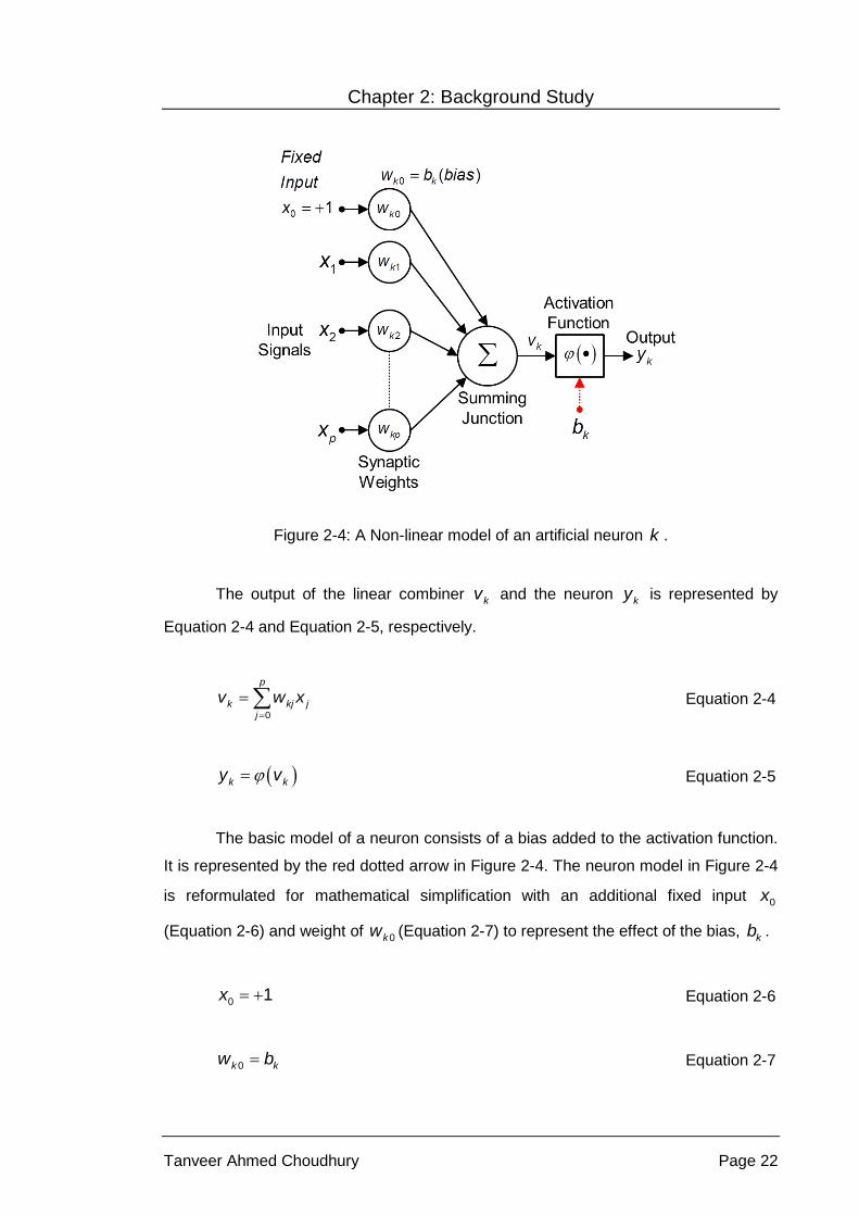
Chapter 2: Background Study
Tanveer Ahmed Choudhury Page 22
Figure 2-4: A Non-linear model of an artificial neuron k .
The output of the linear combiner kv and the neuron ky is represented by
Equation 2-4 and Equation 2-5, respectively.
p
k kj jj
v w x0=
= ∑ Equation 2-4
( )k ky vϕ= Equation 2-5
The basic model of a neuron consists of a bias added to the activation function.
It is represented by the red dotted arrow in Figure 2-4. The neuron model in Figure 2-4
is reformulated for mathematical simplification with an additional fixed input x0
(Equation 2-6) and weight of kw 0 (Equation 2-7) to represent the effect of the bias, kb .
x0 1= + Equation 2-6
k kw b0 = Equation 2-7

Chapter 2: Background Study
Tanveer Ahmed Choudhury Page 23
There are three types of activation function ( )ϕ ; namely threshold function,
piecewise-linear function and sigmoid function.
Equation 2-8 provides the threshold activation function. The output ky of a
neuron k using the threshold activation function is represented by Equation 2-9.
( )v1 if v 00 if v < 0
ϕ≥
=
Equation 2-8
( ) k
k
y k1 if v 00 if v < 0
≥=
Equation 2-9
The piecewise linear activation function is represented by Equation 2-10.
( )v v
11 if v2
1 1 if > v > -2 2
10 if v2
ϕ
≥= ≤ −
Equation 2-10
The sigmoid activation functions are the most common type of activation
functions and exhibit both smoothness and asymptotic properties. Unlike the threshold
activation function, which takes values of only 0 and 1, the sigmoid activation function
assumes a continuous range of values. They are thus differentiable, which is an
important desired feature while designing the ANNs and a reason for their popularity.
Examples of sigmoid functions include the logistic function (Equation 2-11) and the
hyperbolic tangent function (Equation 2-12). The parameter ‘a ’ in Equation 2-11
represents the slope parameter and as the name suggests, it defines the slope of the
function.
( ) ( )v
av1
1 expϕ =
+ − Equation 2-11

Chapter 2: Background Study
Tanveer Ahmed Choudhury Page 24
( ) ( )( )
vvvv
1 exptanh
2 1 expϕ
− − = = + − Equation 2-12
2.2.1.2 Multi-layer feed-forward neural network structure
A schematic of a multi-layer fully connected feed-forward ANN architecture with
two hidden layers is provided in Figure 2-5.
Figure 2-5: Fully connected multi-layer feed-forward artificial neural network
architecture with two hidden layers.
The structure comprises three main sections: the input layer, the output layer
and the layers in between that are termed as the hidden layers. In order to compute
relationships between the inputs and outputs, neurons in the layers between the input
and output are required to perform the ‘intermediate’ computations. Since an observer
only views the input and output layer parameters, and does not see the inputs and
outputs of the intermediate layers of neurons, these layers are termed as the ‘hidden
layer’.

Chapter 2: Background Study
Tanveer Ahmed Choudhury Page 25
The hidden layer is conventionally described as all the other layers, other than
the input and the output layers, consisting of artificial neurons that connect and
establish correlations between the input and output layers. It represents mathematical
functions that are empirically and stochastically derived between the input and output
parameters. The number of hidden layers depends on the type of problem the network
is tasked to solve. The addition of hidden layers allows the network to extract higher-
order statistics [97]. This ability is particularly helpful when the size of the input layer is
large.
The input signal, fed to the network, propagates in the forward direction through
the network on a layer-by-layer basis. This refers to the term “feed-forward” in the
network description. These networks are generally referred to as multi-layer perceptron
(MLP) and have been applied to solve difficult and diverse problems. There are three
distinctive properties of a multilayer perceptron:
1) The model of each neuron in the network contains a smooth (i.e.,
differentiable) nonlinearity at the output end. The presence of nonlinearities
is important because it prevents the input-output relation of the network
getting reduced to that of a single layer perceptron.
2) The network contains one or more layer of hidden neurons that helps the
network to learn complex tasks by extracting progressively useful features
from the input patterns.
3) The network exhibits a high level of connectivity defined by the weights. A
change in connectivity of the network results in a change in the total weight
population.
The multi-layer perceptron generates the superior computing ability through the
combination of these characteristics together with the ability to learn from experience
through training. These characteristics, however, also possess a drawback for the
MLP. The presence of a distributed form of nonlinearity and high network
interconnectivity makes the theoretical analysis of MLP difficult. Secondly, the hidden
layer neurons make visualization of the network difficult.
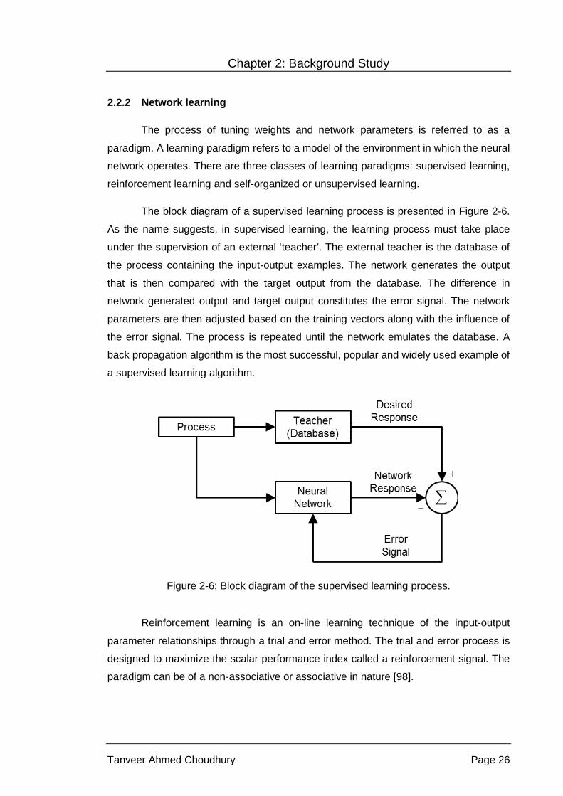
Chapter 2: Background Study
Tanveer Ahmed Choudhury Page 26
2.2.2 Network learning
The process of tuning weights and network parameters is referred to as a
paradigm. A learning paradigm refers to a model of the environment in which the neural
network operates. There are three classes of learning paradigms: supervised learning,
reinforcement learning and self-organized or unsupervised learning.
The block diagram of a supervised learning process is presented in Figure 2-6.
As the name suggests, in supervised learning, the learning process must take place
under the supervision of an external ‘teacher’. The external teacher is the database of
the process containing the input-output examples. The network generates the output
that is then compared with the target output from the database. The difference in
network generated output and target output constitutes the error signal. The network
parameters are then adjusted based on the training vectors along with the influence of
the error signal. The process is repeated until the network emulates the database. A
back propagation algorithm is the most successful, popular and widely used example of
a supervised learning algorithm.
Figure 2-6: Block diagram of the supervised learning process.
Reinforcement learning is an on-line learning technique of the input-output
parameter relationships through a trial and error method. The trial and error process is
designed to maximize the scalar performance index called a reinforcement signal. The
paradigm can be of a non-associative or associative in nature [98].

Chapter 2: Background Study
Tanveer Ahmed Choudhury Page 27
In an unsupervised learning environment, there are no external teachers
present to guide the learning process. Figure 2-7 presents a block diagram of such a
process, which, at times, is also referred to as “self-organizing learning”. The network is
tuned to the statistical regularities of the input data. This develops the network’s ability
to form internal representations for encoding features of the input and create new
classes automatically [99]. As the number of computational layers in the network or the
number of incoming links to a neuron increases, the supervised learning tends to
become unacceptably slow. For such cases, an unsupervised learning process
produces better results.
Figure 2-7: Block diagram of the unsupervised learning process.
2.2.2.1 Back propagation algorithm
A set of well-defined rules for the solution of a learning problem is called the
learning algorithm. The MLP structure (Figure 2-5) has been applied in process
modelling and the most successful supervised learning algorithm used for training such
networks is the back propagation (BP) algorithm [42]. The algorithm is based on the
error-correction learning rule.
The BP algorithm consists of two passes through the different layers of the
network. The first one is the forward pass. In the forward pass, an input vector is
applied to the network. Its effect propagates through the network from layer-to-layer
and finally a set of outputs is generated as network’s actual response. The synaptic
weights of the network are fixed during the forward pass. The second and final pass is
the backward pass, when the synaptic weights of the network are changed and tuned
as per the network’s response during the forward pass and the error correction rule.
The actual network response is subtracted from the target response and the resulting
error signal is then propagated backward through the network against the direction of
the synaptic connections. The synaptic weights are, thus, adjusted to move the
network’s response closer to the desired output.

Chapter 2: Background Study
Tanveer Ahmed Choudhury Page 28
A brief mathematical description of the BP algorithm, in relation to a specific
neuron j , is provided in the following paragraphs. The description is broken down into
two sections. The first section considers the neuron, j , to be an output layer neuron;
while the second case considers the neuron, j , as a hidden layer neuron.
For the first scenario, where the neuron, j , is considered as the output layer
neuron, a signal flow graph of the neuron is presented in Figure 2-8.
Figure 2-8: Signal flow graph of the output layer neuron j.
The error signal value, ( )je n , at the output of neuron j , at a specific iteration
n , is computed using Equation 2-13. ( )jt n and ( )jy n represent the target and actual
response of the neuron j , respectively, at the specific iteration.
j j je n t n y n( ) ( ) ( )= − Equation 2-13
The instantaneous value sum of squared errors is given in Equation 2-14,
where C represents all the output layer neurons. Equation 2-15 provides the average

Chapter 2: Background Study
Tanveer Ahmed Choudhury Page 29
of the sum squared errors with N representing the total number of training samples.
The average squared error value (Equation 2-15) is used as the cost function in
measuring the training performance of the network. The aim of the neural network is to
minimize the value of the cost function by adjusting and optimizing the free parameters
of the network; namely the synaptic weights.
jj C
E n e n21( ) ( )2 ∈
= ∑ Equation 2-14
N
avn
E E nN 1
1 ( )=
= ∑ Equation 2-15
The net internal activity of the neuron j is presented by ( )jv n in Equation
2-16, where p represents the total number of inputs (excluding the fixed value 0 1y =
that represents the effect of bias) applied to the neuron. The synaptic weight, 0jw ,
connected to the fixed input 0 1y = , takes the value of the bias jb applied to the
neuron. The net internal activity of the neuron, j , is finally passed through an
activation function, ( )ϕ , to limit the output signal within a permissible range set for the
model. The final output of neuron j at iteration n is given by ( )jy n (Equation 2-17).
p
j ji ii
v n w n y n0
( ) ( ) ( )=
= ∑ Equation 2-16
( )( )j j jy n v n( ) ϕ= Equation 2-17
For any specific iteration n , the back-propagation algorithm evaluates the
weight correction, ( )jiw n∆ , and applies it to the synaptic weight, ( )jiw n . The weight
correction value is proportional to the partial derivative of the instantaneous sum of
squared errors with respect to the weight value. This provides the instantaneous
gradient, (n) / ( )jiE w n∂ ∂ or the sensitivity factor, determining the direction of weight

Chapter 2: Background Study
Tanveer Ahmed Choudhury Page 30
update. For evaluating the gradient, the chain rule is used to break down the partial
derivative and is represented in Equation 2-18.
j j j
ji j j j ji
e n y n v nE Ew n e n y n v n w n
( ) ( ) ( )(n) (n)( ) ( ) ( ) ( ) ( )
∂ ∂ ∂∂ ∂=
∂ ∂ ∂ ∂ ∂ Equation 2-18
Differentiating both sides of Equation 2-14 with respect to ( )je n gives the value
of (n) / ( )jE e n∂ ∂ .
jj
E e ne n
(n) ( )( )
∂=
∂ Equation 2-19
Differentiating both sides of Equation 2-13 with respect to ( )jy n gives Equation
2-20.
j
j
e ny n
( )1
( )∂
= −∂
Equation 2-20
Differentiating both sides of Equation 2-17 with respect to ( )jv n yields the
value of ( ) / ( )j jy n v n∂ ∂ , presented in Equation 2-21.
( )( )jj j
j
y nv n
v n/( )
( )ϕ
∂=
∂ Equation 2-21
Finally the value of ( ) / ( )j jiv n w n∂ ∂ (Equation 2-22) can be obtained by
differentiating both sides of Equation 2-16 with respect to ( )jiw n .
ji
ji
v ny n
w n( )
( )( )
∂=
∂ Equation 2-22

Chapter 2: Background Study
Tanveer Ahmed Choudhury Page 31
Substituting the solved partial derivatives, from Equation 2-19 to Equation 2-22
in Equation 2-18, gives the instantaneous error gradient (Equation 2-23).
( )( )j j j iji
E e n v n y nw n
/(n) ( ) ( )( )
ϕ∂= −
∂ Equation 2-23
Using the delta rule; the value of weight correction, ( )jiw n∆ , to be applied to
the synaptic weight, ( )jiw n , is computed in Equation 2-24. The negative sign accounts
for the gradient descent of the weight space. The value of η is a constant and gives
the rate of learning.
jiji
Ew nw n
(n)( )( )
η ∂∆ = −
∂ Equation 2-24
Higher value of η results in a steep gradient descent with large changes in the
synaptic weights. Although the speed of the training process is improved in such cases,
the higher value of learning rate might result in an unstable oscillating network. It might
also cause the network to miss the global minimum set for the cost function. In both
cases, the generalization performance of the network is reduced considerably. Setting
this value too low would reduce the steepness of the gradient descent in the weight
space with smaller changes to the synaptic weights from one iteration to the next. The
cost for obtaining such a result is poor training speed. The training process might
become extremely slow making the network impracticable to be used in process
modelling. Adjustment and optimization of the value of η is, thus, critical for the
network’s ability to learn the input-output parameter relationship with sufficient
accuracy.
Substituting the value of (n) / ( )jiE w n∂ ∂ (Equation 2-23) into Equation 2-24
gives a simplified and re-structured value of the weight correction value ( )jiw n∆
(Equation 2-25). The value of j n( )δ in Equation 2-25 represents the local gradient
defined in Equation 2-26.

Chapter 2: Background Study
Tanveer Ahmed Choudhury Page 32
ji j iw n n y n( ) ( ) ( )ηδ∆ = Equation 2-25
( )( )
j jj
j j j
j j j j
e n y nEne n y n v n
n e n v n/
( ) ( )(n)( )( ) ( ) ( )
( ) ( )
δ
δ ϕ
∂ ∂∂= −
∂ ∂ ∂
=
Equation 2-26
With the neuron j set in the output layer, the computations for ( )je n , ( )j nδ
and thus the weight change ( )jiw n∆ is straight forward as shown above. With the
neuron j moved to the hidden layer, the values of ( )je n , ( )j nδ and ( )jiw n∆ need to
be re-calculated, taking into consideration that there is no specified target response for
the neuron. The value of ( )je n cannot be computed using Equation 2-13. This in turn
affects the calculations of ( )j nδ and ( )jiw n∆ in Equation 2-26 and Equation 2-25,
respectively. The following paragraphs illustrate steps for re-computing the updated
weight correction factor ( )jiw n∆ . Figure 2-9 represents an updated version of the
signal flow graph in Figure 2-8, with neuron j used as the hidden layer neuron and an
additional neuron k introduced as the output layer neuron.

Chapter 2: Background Study
Tanveer Ahmed Choudhury Page 33
Figure 2-9: Signal flow graph of the hidden layer neuron j connected to the output layer
neuron k.
Making use of Equation 2-26, the value of local gradient ( )j nδ can be
redefined as in Equation 2-27.
( )( )jj j j
j j j
y nE En v ny n v n y n
/( )(n) (n)( )( ) ( ) ( )
δ ϕ∂∂ ∂
= − = −∂ ∂ ∂
Equation 2-27
The value of the partial derivative (n) / ( )jE y n∂ ∂ in Equation 2-27 is unknown
and needs to be computed. The steps are illustrated below.
From Figure 2-9, the error signal ( )ke n at the output of neuron k , at a specific
iteration n , can be re-written as Equation 2-28. This equation is similar to Equation
2-13, except for the fact the output layer neuron is now represented by k as neuron j
is shifted to the hidden layer. ( )kt n and ( )ky n represent the target and actual
response of the neuron k , respectively.

Chapter 2: Background Study
Tanveer Ahmed Choudhury Page 34
( ) ( ) ( )k k ke n t n y n= − Equation 2-28
In Equation 2-29, ( )kv n (Figure 2-9) represents net internal activity of the
neuron k , where q represents the total number of inputs (excluding the fixed value
0 1y = placed to represent the effect of bias) applied to the neuron. The synaptic
weight 0kw , connected to the fixed input 0 1y = , takes the value of the bias jb applied
to the neuron. The ( )kv n signal is passed through an activation function, ( )kϕ to
generate the final output of neuron k at iteration n is given by ( )ky n (Equation 2-30).
q
k kj jj
v n w n y n0
( ) ( ) ( )=
= ∑ Equation 2-29
( )( )( )k k ky n v nϕ= Equation 2-30
Substituting the value of ( )ky n , obtained from Equation 2-30 into Equation
2-28, we obtain the updated ( )ke n value presented in Equation 2-31.
( )( )( ) ( )k k k ke n t n v nϕ= − Equation 2-31
For the signal flow graph in Figure 2-9, the instantaneous sum of squared errors
from Equation 2-14 can be re-written by just substituting the neuron index j by k .
The updated value is presented in Equation 2-32. ( )ke n represents the error signal at
the output of neuron k (Equation 2-31). Differentiation of (n)E with respect to the
function ( )jy n gives Equation 2-33.
kk C
n e n21( ) ( )2 ∈
Ε = ∑ Equation 2-32

Chapter 2: Background Study
Tanveer Ahmed Choudhury Page 35
kk
kj j
e nE ey n y n
( )(n)( ) ( )
∂∂=
∂ ∂∑ Equation 2-33
Applying the chain rule to the partial derivative ( ) / ( )k je n y n∂ ∂ , Equation 2-33
can be re-written as:
k kk
kj k j
e n v nE e ny n v n y n
( ) ( )(n) ( )( ) ( ) ( )
∂ ∂∂=
∂ ∂ ∂∑ Equation 2-34
Differentiating both sides of Equation 2-31 with respect to ( )kv n gives
( ) / ( )k ke n v n∂ ∂ , presented in Equation 2-35.
( )( )kk k
k
e n v nv n
/( )( )
ϕ∂= −
∂ Equation 2-35
Differentiating both sides of Equation 2-29 with respect to ( )jy n , gives
kkj
j
v n w ny n
( ) ( )( )
∂=
∂ Equation 2-36
Substituting the partial derivatives of k ke n v n( ) / ( )∂ ∂ (Equation 2-35) and
k jv n y n( ) / ( )∂ ∂ (Equation 2-36) in Equation 2-34 gives the value of jE y n(n) / ( )∂ ∂
(Equation 2-37).
( )( )/(n) ( ) ( )( ) k k k kj
kj
E e n v n w ny n
ϕ∂= −
∂ ∑ Equation 2-37
From the definition of local gradient ( )k nδ in Equation 2-26, we can obtain
Equation 2-38.

Chapter 2: Background Study
Tanveer Ahmed Choudhury Page 36
( ) ( )( )/( )k k k kn e n v nδ ϕ= Equation 2-38
Placing the value of ( )k nδ (Equation 2-38) into Equation 2-37, we obtain the
desired partial derivative (Equation 2-39).
(n) ( ) ( )( ) k kj
kj
E n w ny n
δ∂= −
∂ ∑ Equation 2-39
Finally, substituting the partial derivative value of jE y n(n) / ( )∂ ∂ (Equation 2-39)
in Equation 2-27, we obtain the local gradient ( )j nδ for the hidden layer neuron j
(Equation 2-40).
( )( )j j j k kjk
n v n n n/( ) ( )w ( )δ ϕ δ= ∑ Equation 2-40
In Equation 2-40, the function ( )( )j jv n/ϕ depends solely on the activation
function associated with the hidden neuron j . Computation of k n( )δ requires the
knowledge of the error signal ke n( ) for all neurons immediate to the right of the hidden
neuron j and directly connected to neuron j (Figure 2-9). The kj nw ( ) term
represents the synaptic weights associated with these connections.
Summarizing the back propagation algorithm, the weight correction factor
jiw n( )∆ , applied to the synaptic weights connecting neuron i to j , is defined by the
delta rule presented in Equation 2-41. The computation of local gradient j n( )δ
depends on whether the neuron j is the output or hidden layer neuron. For j being
the output layer neuron, j n( )δ equals the product of ( )( )j jv n/ϕ and the error signal
je n( ) associated with neuron j (Equation 2-26). j being a hidden layer neuron,
j n( )δ is the product of ( )( )j jv n/ϕ and the weighted sum of s'δ computed for the
neurons in the next layer connected to neuron j (Equation 2-40).

Chapter 2: Background Study
Tanveer Ahmed Choudhury Page 37
ji j iw n n y n
Learning InputWeight Local
rate signal ofcorrection gradient
parameter neuron j
( ) ( ) ( )
,
η δ∆ = • •
= • •
Equation 2-41
During the training process of a network, the one complete presentation of the
entire training set is represented by an epoch. The learning process is carried out
iteratively epoch by epoch until the cost function of the average squared error, over the
entire training set, converges to its global minimum. In back-propagation, there are two
ways for the learning process to proceed. These are pattern mode and batch mode. In
pattern mode, the weight update is performed after presentation of each of the training
sample (input-output pattern). In the batch learning mode, the weigh update is
performed after presentation of the entire training samples in an epoch.
For the neural network to be used for an on-line operation, pattern mode
learning is preferred as, due to weight update for presentation of each pattern, the
demand for local storage for each synaptic weight is small. In addition to this, in pattern
mode, the input-output examples are generally presented randomly. This feature along
with the use of pattern by pattern updating reduces the change of the algorithm to be
trapped in the local minimum. In the batch learning mode, a more accurate estimate of
the gradient vector is achievable. However there is a greater demand for local memory
for each synaptic weight, as the weight update is performed at the end of each epoch
after the network is presented with all the training data samples. The use of either
pattern or batch learning mode depends on the type of problem the network is required
to solve.
2.2.2.2 Levenberg-Marquardt algorithm
The Levenberg-Marquardt (LM) algorithm is an approximation to Newton’s
method and is designated to reach the second order training speed without computing
the Hessian matrix. The approximation of the Hessian matrix (H) and error gradient (g)
is computed as per Equation 2-42 and Equation 2-43.

Chapter 2: Background Study
Tanveer Ahmed Choudhury Page 38
TH J J= Equation 2-42
Tg J e= Equation 2-43
J represents the Jacobian matrix formed with the first derivatives of the network
errors, e, on the training set with respect to the network’s weights and biases and can
be calculated using the standard back propagation technique [100]. JT is the transpose
of the Jacobian matrix, J.
The LM algorithm uses the approximation in calculation of the Hessian matrix to
update and tune the parameters. If zk represents the old parameter value; then the new
parameter value after calculation of the network errors is given by zk+1 (Equation 2-44).
1
1T T
k kz z J J I J eµ−
+ = − + Equation 2-44
The parameter µ is set to a specific value at the start of the training. After each
epoch, the performance function is computed. If the performance function is found to
be less than the previous epoch then the value of µ is decreased by a specific value.
However, if the performance function increases, the value of µ is also increased by a
specific value. Having the value of µ equal to zero, turns Equation 2-44 into Newton’s
method. The aim is to revert to Newton’s method rapidly since it is faster and more
accurate near an error minimum.
A maximum value of µ is set before the training. If µ reaches its maximum
value, the training stops and indicates that the network has failed to converge. The
training is also stopped when the error gradient (Equation 2-43) falls below a specific
set value or when the goal set for the performance function is met.
The network training steps using the LM algorithm are as follows:
1) All the inputs to the network are presented. The corresponding network
outputs, errors and the sum of square errors, over all inputs are computed.
2) The Jacobian matrix, J, is computed.
3) Equation 2-44 is computed to obtain the new parameter values.

Chapter 2: Background Study
Tanveer Ahmed Choudhury Page 39
4) The sum of squares of errors is recomputed with the updated parameter
values.
5) If the new sum of squares is smaller than the previous value, μ is reduced
by a specific factor β and the process is re-started from step 1.
6) If the new sum of squares is increased, the value of μ is increased by α and
the process is re-started from step 3.
The network is assumed to have converged when the error gradient is less than
some predetermined value or when the sum of squares has been reduced to some
specific error goal.
2.2.2.3 Bayesian regularization algorithm
The Bayesian regularization (BR) algorithm works within the framework of the
LM algorithm and involves modification of the typical performance function during the
training of the feed-forward neural network. The term regularization refers to the
method of improving the generalization ability of a network by constraining the size of
the network weights [101].
Typically the performance function, F, (Equation 2-45) used during network
training, is the average sum of squares of network errors (Equation 2-15).
( )N
avn
F mse E E nN 1
1=
= = = ∑ Equation 2-45
N represents the total number of samples in the training set. E n( ) represents
the instantaneous sum of squared errors of the network and is defined in Equation
2-14.
In regularization, a term consisting of the average of the sum of squares of the
network weights, msw (Equation 2-46), is added to the performance function F
(Equation 2-45) to obtain the new performance function, msereg (Equation 2-47). The
parameter jw in Equation 2-46 represents the network weights.

Chapter 2: Background Study
Tanveer Ahmed Choudhury Page 40
( )n
jj
msw wn
2
1
1=
= ∑ Equation 2-46
( ) ( )msereg mse mswβ α= + Equation 2-47
In Equation 2-47, α and β are the objective function parameters. If the value of
α is much smaller than that of β, the training algorithm will drive the errors to be
smaller. For the opposite condition, the training will emphasize a smoother network
response at the expense of network errors that are generated. The critical challenge in
regularization is the selection of appropriate values of α and β. Application of the
Bayesian rule is performed [101] to neural network training and optimizing
regularization with reference to selection of the optimal objective function parameters.
The steps in network training and Bayesian optimization of the regularization
parameters [102], within the LM algorithm framework, are presented below:
1) The values of α and β are initialized to 0 and 1, respectively. The weights
were initialized using the Nguyen-Widrow method [103].
2) The LM algorithm is used to minimize the performance function in Equation
2-47 and update the weight matrix accordingly.
3) The effective number of parameters is computed using the Gaussian
Newton approximation to the Hessian matrix available in the LM training
algorithm.
4) New estimates of the objective function parameters α and β are computed.
5) Steps 2 to 4 are iterated until the error converges.
The BR algorithm uses a regularization technique to combat the problem of
over-fitting. The algorithm, thus, uses the whole available dataset for training purposes
without any need for a separate validation set. This method prevents data from being
discarded and maximizes the volume of training data. The algorithm particularly suites
cases where there is a relatively small dataset available for network training.
Furthermore, BR preserves an optimal network size and reduces the pre-training work
required to determine the minimum network size to avoid over-fitting.

Chapter 2: Background Study
Tanveer Ahmed Choudhury Page 41
2.2.2.4 Resilient back propagation algorithm
The Resilient Back Propagation (RBP) algorithm eliminates the harmful effects
of the magnitudes of the partial derivatives. Only the sign of the derivative determines
the direction of weight update. The size of the weight change is determined by a
separate update parameter. The update parameter value for each weight and bias is
increased by a specific factor when the derivative of the performance function, with
respect to that of weight, has the same sign for two successive iterations. The update
value is decreased by a factor when the derivative, with respect to that of weight,
changes sign from the previous iteration. If the derivative is zero, the update value
remains the same. Whenever the weights fluctuate, the weight change is reduced. If
the weight continues to change in the same direction for several iterations, the
magnitude of the weight change increases. A detail study of the algorithm is provided in
the reference [104].
2.3 Multi-Net system
A modular combination of the multi-net system is used in Section 4.2 of Chapter
4 to model the APS process and predict the in-flight particle characteristics from the
input processing parameters. Modular implementation allows simplification of the
optimized model structure with enhanced ability to generalise the network. It achieves
better correlations between each of the in-flight particle characteristics with the input
processing parameters. The modular combination concept is new to the field of thermal
spray processes. Applications of any multi-net system in modelling the APS process
have not been reported; therefore, background information is presented as follows.
A multi-net system [105] is a group of ANNs where each network, depending on
the type of combination, is assigned to solve a part of the problem or the total problem.
The original problem is decomposed into sub-problems and each network focuses on
solving a sub-problem. Decomposition of the task makes it easier to understand and
modify. The use of a multi-net system improves the generalization ability of the ANN,
i.e. to correctly respond to inputs that were not used to adapt the network’s weights. A
multi-net system generally provides solutions to problems that either cannot be solved
by a single net, or which can be solved more effectively by a system of modular neural
net components. Similarly, better performance is achieved by the introduction of
redundancy in the number of network.

Chapter 2: Background Study
Tanveer Ahmed Choudhury Page 42
There are two combinations of ANNs in a multi-net system [106]: (i) ensemble
combination, and (ii) modular combination. Figure 2-10 gives a pictorial view of the
different classifications of multi-net systems at both task and sub-task levels.
‘Ensemble’ is the commonly used term for combining a set of redundant nets
[107]. In an ensemble combination, each component nets provide a complete solution
to the same task or task components. Each of these solutions might be different to
each other. A final solution is obtained by decision fusion of the solutions of the
redundant component nets. However, in modular approach no redundancies exist for
the component nets. The task is decomposed into subtasks. Each module is provided
with a subtask, for which it provides a solution. The complete task solution is obtained
by combination of all the modules output. In this study, a module is referred to as a self
– contained or autonomous processing unit [108].
Figure 2-10: Classifications of a multi-net artificial neural network system.

Chapter 2: Background Study
Tanveer Ahmed Choudhury Page 43
Both the ensemble and modular combinations can exist at the task or sub-task
level. In the task level, an ensemble can consist of a number of different solutions to an
entire task. Similarly, the task could be split into different sub-tasks and fed into
different modules. The task solution is then constructed from the combination of the
decomposed modules. In the sub-task level, when a task is broken down into
component modules, each component can itself consist of an ensemble of nets with
each generating a solution for the same modular component. Alternatively, each
module can be further subdivided into more specific modules. At both levels, the
difference between an ensemble and modular combination is the presence or absence
of redundancy in the number of component networks. There are always redundancies
for ensemble combinations, while a lack of it for modular combination.
Modular and ensemble combinations are not mutually exclusive and a multi-net
system could consist of a mixture of ensemble and modular combinations at different
levels. Both approaches work with the aim of improving the generalization performance
of the networks and both can involve linear combination of their components. However,
the modular combination assumes that each data point is assigned to only one expert
(i.e., it is mutual exclusive) whereas ensemble combination makes no such assumption
and each data point is likely to be dealt with by all the component nets in an ensemble.
2.3.1 Ensemble combination
Combining networks in redundant ensembles helps to improve the
generalization ability. Combination of a set of imperfect estimators is a way to manage
limitations of the individual estimators. The effect of the errors made by each
component net can be reduced by proper combinations. A forecasting study in
reference [109] showed that better results can be achieved by combining forecasts
instead of choosing the best one. Introduction of redundancy and multiple versions is a
standard method in software engineering to increase the reliability [110].
2.3.1.1 Creating ensembles
There is no advantage in combining nets in ensembles that are composed of a
set of identical nets since the identical nets generalize in the same way. The main
emphasis is placed on the similarity or on the pattern of generalization. In principle, the
same solution can be obtained from a set of networks that vary in terms of their

Chapter 2: Background Study
Tanveer Ahmed Choudhury Page 44
weights, convergence time and architecture (e.g., number of hidden layers). This is
primarily because the networks generated the same pattern of errors when tested on a
test set. The aim is to obtain networks that generalize differently. A number of training
parameters can be varied and manipulated to make the network generalize differently.
The parameters include: initial conditions, the topology of the nets, the training
algorithm and the training data. A brief overview of each is provided below:
1) Initial weights: Keeping the training data constant, a set of networks can be
created, with each having different initial random weights.
2) Topology: A set of networks can be created having different network
topology or architecture. The networks are trained with a different number of
hidden layers and the same training data. Errors generated by two networks
with different network topology are likely to be uncorrelated.
3) Training Algorithm: A set of networks can be created and trained with a
different training algorithm and the same data.
4) Training Data: A set of networks can be created by altering the training data.
This can be done in a number of different ways outlined below. Ensembles
could be created using one of these factors individually or combining two or
more of these techniques.
a. Sampling Data: A common approach in the generation of a group of
networks for an ensemble is to train each net with a different
subsample of the training data. Cross-validation [111] and
bootstrapping [112] are resampling methods used for this purpose.
b. Disjoint Training Set: The method includes training each network in
the ensemble set with disjoint or mutually exclusive training sets
[113]. There is no overlap in the different training data sets; however,
the size of the set might reduce and result in poor generalization
performance [114].
c. Boosting and Adaptive Resampling: A boosting algorithm is an
effective method in varying the training data for various ensemble
nets. However, the main disadvantage of the algorithm is that it
requires a large amount of data [115]. The Freund and Schapire

Chapter 2: Background Study
Tanveer Ahmed Choudhury Page 45
algorithm [116] overcomes the difficulty by adaptively resampling the
training sets such that the weights in the resampling are increased
for those cases that are most often misclassified.
d. Different Data Source: The method includes having the training data
from different input sources. A similar example is relayed in study
[113].
e. Pre-processing: Various pre-processing techniques, such as pruning
[114] or the use of non-linear transformations [117], can be used to
vary the training data of the networks.
2.3.1.2 Combining Ensemble Nets
There are various methods of combining the created ensembles effectively
[118-121]. A brief outline of the methods is provided below.
1) Averaging and Weighted Averaging: A single network output can be created
from a set of ensemble network outputs by simple averaging [122] or
weighted averaging, which takes into account the relative accuracies of the
nets to be combined [122-124].
2) Non-Linear Combining Methods: The non-linear methods used for
combination of ensemble networks include Dempster-Shafer belief based
methods [125], combination using rank based information [126], voting [107]
and order statistics [127].
3) Supra Bayesian: In the supra Bayesian approach, the opinions of the expert
networks are considered themselves as data; thereby allowing the
probability distribution of the experts to be combined with its own prior
distribution.
4) Stacked Generalization: The non-linear network combines the networks with
weights that vary over the feature space [128]. This term is used to refer
both to this method of stacking classifiers and also to the method of creating
a set of ensemble networks trained on different partitions of the data. A
detailed study on stacking is reported in [129].

Chapter 2: Background Study
Tanveer Ahmed Choudhury Page 46
2.3.2 Modular combination
Modular approaches are used for improving the performance of a task. The task
can be accomplished with a monolithic network. However, breaking down the tasks into
specialist modules provides better performance. This approach is also used for tasks,
which might not be possible to accomplish, unless the problem is simplified by
decomposition. The ‘divide and conquer’ principle is applied to extend the capabilities
of a single net. The task is divided into a number of sub-problems, where each sub-
problem is then solved with a different ANN architecture and algorithm. This process
allows the system to exploit specialist capabilities. The study in [130] reports a problem
in robotics, whose solution was only obtained as a result of decomposing the task into
three separate components. A similar problem in laid out in study [131]. The solution to
a language parsing task; i.e., mapping from syntactically ambiguous sentences to a
disambiguated syntactic tree was only obtained by decomposing the task into different
modules.
Each module in a modular system can be in the form of an ANN. However, in
principle, some of these components can use non-neural computing techniques. A
study in [132] provides details of a hybrid combination of a knowledge based system
and an ANN. In the field of speech recognition, use of hybrid system architectures is
common [133]. The pre-processing of ANN input before training can also be
considered as a form of modular decomposition for the purpose of simplification of the
problem.
Apart from improving the performance of the ANNs, a reason behind adopting a
modular approach is to reduce model complexity. It helps in making the overall system
easier to understand, modify and extend [134]. Training times can also be reduced
[135] and previous knowledge can be incorporated in terms of suggesting an
appropriate decomposition of a task [134].
2.3.2.1 Creating modular components
In modular combination, decomposition of the task into modular components
can be achieved automatically, explicitly or by means of class decomposition [136].
Explicit decomposition of the modules is performed when there is a strong
understanding of the problem. The division is performed before the training [137] and

Chapter 2: Background Study
Tanveer Ahmed Choudhury Page 47
an improved learning performance can be achieved [138]. In the similar manner,
specialist modules might be developed for particular purposes. At times, the modules
provide specialist solution to the same task such that the best performance on the task
will be obtained when the most appropriate module is selected. In the study [139], the
neural net modules were separately optimized to either reduce the number of false
positive errors or the number of false negative errors. Explicit decomposition was
carried out for complex structures with the aim of improving performance or
accomplishing tasks that either could not be accomplished using a monolithic network
or as easily or naturally.
Class decomposition splits a problem into sub-problems based on the class
relationships. The method [140] involves dividing a k-class classification problem into k
two-class classification problems. The division is performed using the same number of
training data for each two class classification as the original k-class problem. The study
[136] reports a further refinement of the problem.
The automatic decomposition of the task is characterized by the blind
application of a data partitioning technique. It is generally carried out in order to
improve performance of the networks. Complex problems are automatically
decomposed into set of similar problems under the divide and conquer approach of
Jacobs and Jordan [141-143].
2.3.2.2 Combining modular components
There are at least four different modes of combining component nets; namely,
co-operative, competitive, sequential and supervisory. Figure 2-11 shows the four
modes of combination.

Chapter 2: Background Study
Tanveer Ahmed Choudhury Page 48
Figure 2-11: Four different modes of combining artificial neural network modular
components (a) cooperative combination, (b) sequential combination, (c) competitive
combination, and (d) supervisory combination.
The study [106] classed the co-operative and competitive combinations
together. However, there is a difference in which they combine. In co-operative
combination, some contribution to the decision is assumed to be made by each of the
elements combined. Whereas, in competitive combination, for each of the inputs, the
most appropriate element is assumed to be selected. There are two mechanisms
governing the selection under competitive combination.

Chapter 2: Background Study
Tanveer Ahmed Choudhury Page 49
1) Rule 1: Gating: Expert modules are combined by means of a gating net
[141, 142]. The system is trained to allocate examples to the most
appropriate module.
2) Rule 2: Rule-based Switching: Switching between modules is triggered by
means of explicit mechanisms on the basis of the input. An example of a
form of rule-based switching is provided in the study [139] where, depending
on one of the model’s output, the control is switched between modules.
There are two networks separately optimized in a way that one makes
fewest possible false positive errors and the other generates fewest
possible false negative errors. The output of the first network is used. The
output of the second is only used when the output exceeds an empirically
defined threshold [144].
Sequential combination entails successive processing and the computation of
one module depends on the output of the preceding module. Under the supervisory
relationship, one module is used to supervise the performance of another module.
McCormack [145] describes a system where the parameters of the second network are
selected based on the observations of various parameter values on the performance of
the first network. Another example of a supervisory relationship [146] shows where the
input features and the output of the main ANN module is used to train a supplementary
network to predict the error of a main network.

Chapter 3 Artificial Neural Network
Modelling

Chapter 3: Artificial Neural Network Modelling
Tanveer Ahmed Choudhury Page 51
Chapter 3 Artificial Neural Network Modelling
Work presented in this chapter has been published in the following journal and
conference papers:
T. A. Choudhury, N. Hosseinzadeh, and C. C. Berndt, "Improving the
Generalization Ability of an Artificial Neural Network in Predicting In-Flight Particle
Characteristics of an Atmospheric Plasma Spray Process," Journal of Thermal Spray
Technology, vol. 21, pp. 935-949, 2012.
T. A. Choudhury, N. Hosseinzadeh, and C. C. Berndt, "Artificial Neural
Network application for predicting in-flight particle characteristics of an atmospheric
plasma spray process," Surface and Coatings Technology, vol. 205, pp. 4886-4895,
2011.
T. A. Choudhury, N. Hosseinzadeh, and C. C. Berndt, "Using Artificial Neural
Network to predict the particle characteristics of an Atmospheric Plasma Spray
process," in International Conference on Electrical and Computer Engineering (ICECE),
Dhaka, 2010, pp. 726-729.
3.1 Background
This chapter illustrates the different stages of the artificial neural network (ANN)
modelling of the atmospheric plasma spray (APS) process in predicting the in-flight
particle characteristics from the input processing parameters. One of the major
problems for such a function-approximating neural network is over-fitting, which
reduces the generalization capability of the trained network and its ability to work with
sufficient accuracy under a new environment. Two methods are used to analyse the
improvement in the network’s generalization ability: (i) cross-validation and early
stopping, and (ii) Bayesian regularization. Figure 3-1 presents a flow chart to present
the overall research methodology.
The chapter starts with describing the data collection and processing steps
followed by the database expansion procedure. It is followed by the ANN model build
up, training and optimization steps. Simulations are performed both on the original and
expanded database with different training conditions to obtain the variations in
performance of the trained networks under various environment. The simulation results
obtained from the various network models are discussed and analysed. The chapter

Chapter 3: Artificial Neural Network Modelling
Tanveer Ahmed Choudhury Page 52
further studies the predicted values, with respect to the experimental ones, to evaluate
the performance and generalization ability of the network. It helps in analysing the
parameter relationships and correlations. The simulation results show that the
performance of the trained networks with regularization is improved over that with
cross-validation and early stopping. Furthermore, the generalization capability of the
networks is improved; thus preventing and phenomenon associated with over-fitting. A
summary of the work is presented at the end of the chapter.
Figure 3-1: Research methodology for artificial neural network modelling of the
atmospheric plasma spray process.

Chapter 3: Artificial Neural Network Modelling
Tanveer Ahmed Choudhury Page 53
3.2 Data collection and pre-processing
An important step in artificial neural network modelling involves the database
collection, pre-processing the data and assessing the outputs. A robust and sufficiently
large database is essential for the construction of a network that generalizes well. A
database from the open literature (DSO in Table 3-1) [40] was used in this work. This
database was built experimentally by observing the effect of the relevant APS input
processing parameters on the in-flight Al2O3-13 wt. % TiO2 particle characteristics.
The authors of Ref. [40] measured the in-flight dynamic behaviour of the
particles from the centre of the particle flow stream using a dichromatic sensor (DPV –
2000 from TECNAR Automation Limited, St-Bruno, QC, Canada J3V 6B5). This data
was processed to create a database (DSO) of the average particle velocity, temperature
and diameter for each of the input conditions.
The APS input processing parameters include the following six power and
injection parameters: (i) arc current intensity, (ii) argon primary plasma gas flow rate,
(iii) hydrogen secondary plasma gas flow rate, (iv) argon carrier gas flow rate, (v)
injector stand-off distance, and the (vi) injector diameter. The output parameters
consist of the following in-flight particle characteristics: (i) the average particle velocity,
(ii) temperature, and (iii) diameter.
The in-flight particle characteristics of the plasma jet govern the type, nature
and characteristics of the coatings and are particularly sensitive to the selected six
input processing parameters. Other input parameters of the plasma spray process,
such as those parameters related to powder injection, the type of torch, the spray
distance and the torch movement, which do not have a significant influence on the in-
flight particle characteristics [16, 17], were kept constant to their reference values. This
limits the validity of the model to the investigated cases only.
The database, DSO, contains 16 data values. The variations of the input
processing parameters in Table 3-1 are presented as bold numbers. A single input
processing parameter was varied at any time. The remaining parameters were fixed at
their reference values. This allows in understanding the effect of the variations of each
of the input processing parameters on the in-flight particle characteristics. The
reference values of the input processing parameters are noted later in Table 3-2.

Chapter 3: Artificial Neural Network Modelling
Tanveer Ahmed Choudhury Page 54
Table 3-1: Experimental database (DSO) from literature consisting of the atmospheric
plasma spray input processing parameters and the output in-flight particle
characteristics [40].
Run I [A]
ArV[SLPM]
2HV[SLPM]
CGV[SLPM]
injD [mm]
ID[mm]
Experimental Values
V [m/s]
T [°C]
D [μm]
1 350 40 14 3.2 6 1.8 242 2,262 43
2 530 40 14 3.2 6 1.8 270 2,399 51
3 750 40 14 3.2 6 1.8 278 2,428 50
4 530 40 0 3.2 6 1.8 205 1,675 30
5 530 40 4 3.2 6 1.8 241 2,170 38
6 530 40 8 3.2 6 1.8 260 2,351 45
7 530 40 10 3.2 6 1.8 264 2,373 47
8 530 45 15 3.2 6 1.8 176 2,403 51
9 530 22.5 7.5 3.2 6 1.8 179 2,456 49
10 530 37.5 12.5 3.2 6 1.8 263 2,393 50
11 530 40 14 2.2 6 1.8 252 2,352 48
12 530 40 14 4.4 6 1.8 277 2,440 54
13 530 40 14 3.2 7 1.8 270 2,434 47
14 530 40 14 3.2 8 1.8 278 2,451 52
15 530 40 14 3.2 6 1.5 265 2,498 54
16 530 40 14 3.2 6 2 278 2,363 43
I Current Intensity
ArV Argon primary plasma gas flow rate
2HV Hydrogen secondary plasma gas flow rate
CGV Argon carrier gas flow rate
injD Injector stand-off distance
ID Injector diameter
V Average in-flight particle velocity
T Average in-flight particle temperature
D Average in-flight particle diameter

Chapter 3: Artificial Neural Network Modelling
Tanveer Ahmed Choudhury Page 55
The values of the input processing parameters and the output in-flight particle
characteristics require a linear transformation before being used for any ANN training
and testing purposes. This normalization procedure ensures equal treatment from ANN
in handling and processing the data. It also prevents any calculation error related to
different parameter magnitudes. The values are normalized using Equation 3-1 [38]
−
=−
MINNORM
MAX MIN
X XXX X
Equation 3-1
NORMX stands for the normalized parameter value, MAXX and MINX are the
maximum and minimum possible values of the parameters based upon their physical
limitations of the process, not from the experimental sets. The physical limits of each
input and output variable are given in Table 3-2 [40].

Chapter 3: Artificial Neural Network Modelling
Tanveer Ahmed Choudhury Page 56
Table 3-2: Physical limits of the atmospheric plasma spray input processing
parameters and the output in-flight particle characteristics along with the input
parameters reference values [40].
Variable Lower Limit
Highest Limit
Reference Value
Current Intensity, I [A] 303 840 530
Argon Plasma Gas Flow Rate, ArV [SLPM] 20 44 40
Hydrogen Plasma Gas Flow Rate, 2HV [SLPM] 0 17 14
Carrier Gas Flow Rate, CGV [SLPM] 2 5 3.2
Injector Diameter, ID [mm] 1.5 2 1.8
Injector Stand-off Distance, injD [mm] 6 8 6
Average In-Flight Particle Velocity, V [m/s] 122 408 …
Average In-Flight Particle Temperature, T [°C] 1,236 3,240 …
Average In-Flight Particle Diameter, D [μm] 14 101 …
3.3 Database expansion
An artificial sequence of input-output vectors was created with the view of
expanding the database. The expanded database, when used for network training, is
expected to combat the problem of over-fitting and produce a network with good
generalization ability. In this study, kernel regression [147] is used for the expansion of
the database. Additive white Gaussian noise is added to each of the input-output
training vectors based on the Parzen-Rosenblatt estimate [148-150] of the true input –
output vector density.
The kernel estimate, also called the Parzen-Rosenblatt estimate, is a non-
parametric way of estimating the probability density function of a random variable. As

Chapter 3: Artificial Neural Network Modelling
Tanveer Ahmed Choudhury Page 57
an illustration, from some sample data of a population, kernel estimation allows
extrapolation of the data to the entire population. Let x be a random number in the
Euclidean space dR and the distribution of x is described by the probability density
function f . Suppose K be the kernel in the d-dimensional space and nh a smoothing
parameter called the bandwidth, taking values greater than 0. Now if 1, , nX X are
samples of n independent observations of X , then the n-point kernel estimate of f
corresponding to K and h is:
( )=
−= ∈
∑,
1
1 1 ,n
din h d
i n n
x Xf x K x Rn h h
Equation 3-2
The characteristics of the additive noise are controlled by the parameters K
and h . For kernel density approximation, the Gaussian probability density function
(PDF) is used. With mean of 0 and variance 1, the Gaussian kernel becomes,
( )
π
−−− =
2
2212
ix Xi hx XK e
h Equation 3-3
( )( )
π
−−
=
= ∑2
22,
1
1 12
ix Xnh
n hi
f x en h
Equation 3-4
From Equation 3-4, we find that the value of the bandwidth h indirectly controls
the variance of the Gaussian PDF along each dimension.
Kernel regression is a non-parametric technique in statistics to estimate the
conditional expectation of a random variable without assuming any underlying
distribution to estimate the regression function [151]. The idea is to map an identical
kernel, which is the Gaussian kernel (Equation 3-5) in this case, local to each
observation data point. The kernel assigns weight, w , to each location based on
distance from the data point. The function depends only on the width from the local
data point to a set of neighbouring locations. By inserting Gaussian kernels in the
Chapter 3: Artificial Neural Network Modelling
Tanveer Ahmed Choudhury Page 58
original data iX , the value of the original data is extended to a much smaller value at a
certain small step of dx .
( )−
−=
2
2( )
2,ix X
hh iK x X e Equation 3-5
The kernel values are computed for each data point iX . Then, the estimated
value of jy at domain value jx is computed according to the kernel regression formula
(Equation 3-6), also called the Nadaraya – Watson kernel weighted average.
( )
( )=
=
=∑
∑1
1
,
,
n
i h j ii
j n
h j ii
w K x Xy
K x X Equation 3-6
The nominator of the kernel regression formula (Equation 3-6) is an array of the
sum of the products of the Gaussian kernels (Equation 3-5) and the weight. The
denominator is the sum of the kernel values at domain jx for all data points iX . With
the computed value of y , the sum square error (SSE) is calculated by comparison with
the original iY data. The associated weights are optimized for each kernel to minimize
SSE. The regression is solved by computing the estimated values of y with the new
array of weights. Tabulating all the values of domain x and the corresponding
estimated values of y gives rise to the expanded database DSE, tabulated in
Appendix B. The expanded database, DSE, is approximately nineteen times the original
database (DSO).
For the purpose of testing the generalization performance of the trained
networks, 20% of the expanded database, DSE, is selected by an interleaving process
as the test set. This is called “DSET”. Interleaving insures that the test data set
represents an overall view and statistical representation of the whole database. The
remaining 80% of the data are set aside as a training set (called “DSETR”) used for
network training and optimization purposes. Similarly, 20% of the original database

Chapter 3: Artificial Neural Network Modelling
Tanveer Ahmed Choudhury Page 59
DSO is selected by interleaving as the test set (DSOT) and the remaining 80% of the
data as the training set (DSOTR).
3.4 Network architecture
A simple ANN model considering the multi-layer perceptron (MLP) approach
and based on a back propagation algorithm is used in this section. This permits the
prediction of a complex non-linear relationship between the input processing
parameters and the output in-flight particle characteristics [42] present in the database
generated experimentally from the APS process.
The block diagram of the designed ANN is presented in Figure 3-2.
Figure 3-2: Block diagram of the designed multi-layer artificial neural network.

Chapter 3: Artificial Neural Network Modelling
Tanveer Ahmed Choudhury Page 60
In Figure 3-2, jiw (where i = 1…8 and j = 1…N1) represents the input layer
weights. The terms α ji (where i = 1… N1 and j = 1… N2) and β ji (where i = 1…N2 and
j=1…3) represent the hidden layer weights and output layer weights, respectively. 1N
and 2N represents the number of linear nodes or neurons in hidden layer 1 and hidden
layer 2.
There exists no generalized rules to specify the exact values of 1N and 2N . The
number depends on the nature of the problem that the network encounters and the
network optimization process. The large number of hidden layer neurons provides
network flexibility to optimize many parameters and reach an improved solution.
However, increasing the size of the hidden layer over a certain limit makes the network
under-characterized. The network in such cases is forced to optimize more parameters
than the data vectors available to define these parameters. Too few a number of
neurons in the hidden layers leads to under-fitting. The performance of a trained ANN
is sensitive to the size of the hidden layers and the optimum number and combination
of neurons in the hidden layers are determined from the network training and
optimization process.
The multi-layer architecture comprises three parts: the input layer, the hidden
layers and the output layer (Figure 3-2). The number of data points required to define
each of the input parameters depends on the nature of the parameter. One data point
is required to represent a real valued parameter and x data points are required to
describe x2 classifications or categories [39].
In this study, only the parameters of (i) injector diameter ( )ID and (ii) injector
stand-off distance ( )injD represented classifications with three distinct values and
were, thus, described by two data points each (Table 3-3). All the other input variables,
which includes current intensity, argon primary plasma gas flow rate, hydrogen
secondary plasma gas flow rate and argon carrier gas flow rate, are continuous real
valued parameters and were represented by one data point each. The input layer thus
consisted of 8 data points. The same rule was applied to define the number of neurons
for each output parameters. The output layer had 3 neurons as all the output
parameters were real valued parameters and were represented by one neuron each.
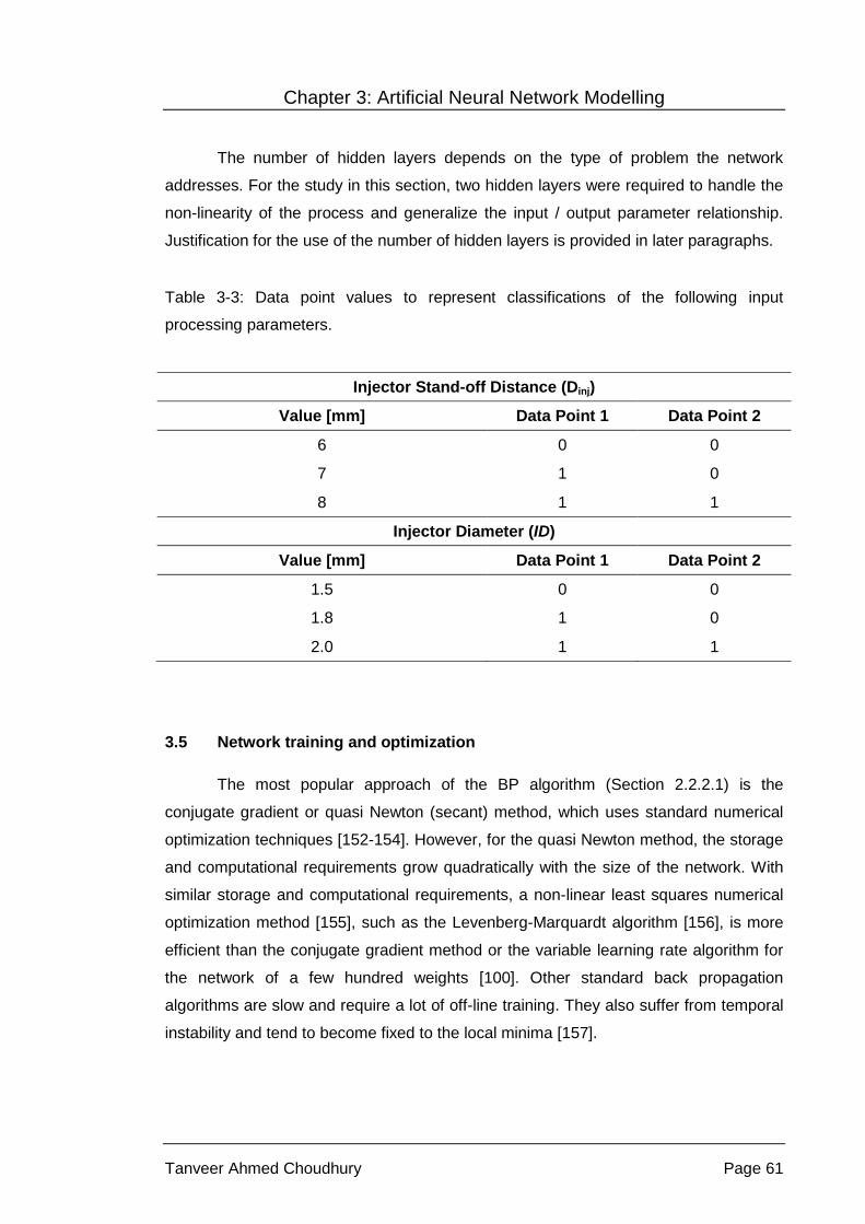
Chapter 3: Artificial Neural Network Modelling
Tanveer Ahmed Choudhury Page 61
The number of hidden layers depends on the type of problem the network
addresses. For the study in this section, two hidden layers were required to handle the
non-linearity of the process and generalize the input / output parameter relationship.
Justification for the use of the number of hidden layers is provided in later paragraphs.
Table 3-3: Data point values to represent classifications of the following input
processing parameters.
Injector Stand-off Distance (Dinj)
Value [mm] Data Point 1 Data Point 2
6 0 0
7 1 0
8 1 1
Injector Diameter (ID)
Value [mm] Data Point 1 Data Point 2
1.5 0 0
1.8 1 0
2.0 1 1
3.5 Network training and optimization
The most popular approach of the BP algorithm (Section 2.2.2.1) is the
conjugate gradient or quasi Newton (secant) method, which uses standard numerical
optimization techniques [152-154]. However, for the quasi Newton method, the storage
and computational requirements grow quadratically with the size of the network. With
similar storage and computational requirements, a non-linear least squares numerical
optimization method [155], such as the Levenberg-Marquardt algorithm [156], is more
efficient than the conjugate gradient method or the variable learning rate algorithm for
the network of a few hundred weights [100]. Other standard back propagation
algorithms are slow and require a lot of off-line training. They also suffer from temporal
instability and tend to become fixed to the local minima [157].

Chapter 3: Artificial Neural Network Modelling
Tanveer Ahmed Choudhury Page 62
Thus, taking into consideration that the network size dealt in this work is within
a few hundred weights, the initial back propagation paradigm selected for the ANN
training and optimization purpose was the Levenberg-Marquardt algorithm (Section
2.2.2.2). With the Levenberg-Marquardt (LM) algorithm, cross-validation and early
stopping statistical techniques were applied to train the neural network. The Bayesian
regularization (BR) algorithm (Section 2.2.2.3) was later used to replace the LM
algorithm using cross-validation and early stopping to view further changes in the
generalization ability of the neural network.
Initially it was important to determine the optimal number of hidden layers.
Simulation was started with one hidden layer. The maximum number of allowed epochs
for each training cycle was set to 10,000. This ensured that the network was allowed to
train for sufficient time until the error gradient converges completely or any pre-defined
stopping criteria were reached. The transfer function used in all layers in the log-
sigmoid function and the error performance function was set to a mean absolute error
(MAE) (Equation 3-7).
=
= ∑1
1 n
iMAE PredictedValue-TrueValue
n Equation 3-7
The number of neurons in the hidden layer was varied from four to twenty with
increment of one neuron. For each case, the network was trained several times with
the database DSETR and the network generating maximum correlation coefficient, R,
value on the test set, DSET, was stored and saved. Details regarding the correlation
coefficient (R) are discussed later in this chapter. The average MAE value was also
computed for all the networks.
The number of hidden layers was increased to two and the number of neurons
in each layer was varied from four and three (4-3) to twenty and nineteen (20-19),
respectively. The network training and performance measurement was repeated as
above. Similar simulations were performed for three and four hidden layer networks.
For the networks with three hidden layers, the number of neurons in each layer was
varied from four, three and two (4-3-2) to twenty, nineteen and eighteen (20-19-18),
respectively. Finally for the networks with four hidden layers, the number of neurons in
each hidden was varied from four, three, two and one (4-3-2-1) to twenty, nineteen,

Chapter 3: Artificial Neural Network Modelling
Tanveer Ahmed Choudhury Page 63
eighteen and seventeen (20-19-18-17), respectively. In all the cases with two, three
and four hidden layers, the number of neuron, in each hidden layer, was increased by
one.
Figure 3-3 provides a summary of the performance comparison of the networks
having a different number of hidden layers and trained with two algorithms. The
network with two hidden layers generated the minimum error when trained with both
algorithms. Considering the results obtained from Figure 3-3, along with the non-
linearity associated with the process under consideration in this work , the number of
hidden layers in the designed ANN is set to two (Figure 3-2).
Figure 3-3: Network performances with different algorithms and number of hidden
layers.
Before starting the ANN training, all the network weights and parameters were
initialized to random values. The error performance function was re-set to mean square
error (MSE) (Equation 2-45). The number of neurons in the first and second hidden
layer was initially set to four and three neurons, respectively. The ANN was first trained
with the Levenberg-Marquardt algorithm along with cross-validation and early stopping.
It was first presented with the dataset DSOTR.

Chapter 3: Artificial Neural Network Modelling
Tanveer Ahmed Choudhury Page 64
A large number of training data is essential to enhance the level of accuracy of
a trained network. However, at the same time, it is also important to have a sufficiently
large validation set to investigate the generalization ability of the designed model.
Thus, the number of samples to be assigned in each of the subsets is an important
consideration. The dataset, DSOTR, is divided by interleaving two subsets: the training
set and the validation set. The data division ratio (training set: validation set) is set to
0.90:0.10, 0.85:0.15, 0.80:0.20, 0.75:0.25 and 0.70:0.30. The standard deviations of
the training and the validation set were computed. The bar chart depicting absolute
differences between the standard deviations of the training set and the validation set is
shown in Figure 3-4. From the analysis, a data division ratio of 0.85:0.15 was chosen,
since the difference in standard deviations was the least. This result depicts the training
and validation sets being statistically most similar to each other in terms of data
variations and fluctuations and provides a strong base to training a network having
good generalization ability.
The network was trained several times. After each of the training cycles, the
trained network was simulated with the test set DSOT. The network producing maximum
correlation coefficient (R) values on the test set was stored and saved along with the
MSE values. The combination of the number of neurons in each of the hidden layers
was varied several times and the whole process repeated.

Chapter 3: Artificial Neural Network Modelling
Tanveer Ahmed Choudhury Page 65
Figure 3-4: Difference in standard deviations of the training and validation sets for
DSOTR.
The database was then replaced with DSETR. The data was again interleaved
into training and validation set and the data division ratio was set to 0.90:0.10,
0.85:0.15, 0.80:0.20, 0.75:0.25 and 0.70:0.30. The standard deviations of the training
and the validation set are computed and their absolute difference is presented below in
Figure 3-5. The data division ratio of 0.80:0.20 was chosen for having the lowest
deviations between the standard deviations of the sets. The network was once again
trained and validated with the same combination of the number of hidden layer neurons
used previously for training the network with database DSOTR. For each combination of
the number of neurons in the hidden layer, the network training procedure was
repeated several times as before. The network generating the maximum R-value on
the test set DSET was stored and saved with their respective MSE values.

Chapter 3: Artificial Neural Network Modelling
Tanveer Ahmed Choudhury Page 66
Figure 3-5: Difference in standard deviations of the training and validation sets for
DSETR.
The MSE generated by the network when simulated with an unseen data set
provides a measure of the ‘generalization error’ or the performance of the trained
network. For this study the unseen set is the test set, whose values were not presented
to the network during the training process. The lower this error, than the better is the
network’s performance and ability to generalize the process and predict with sufficient
accuracy under unseen environments.
Table 3-4 provides a table of all the generalization errors generated by the
networks. When compared with the performance of the networks trained with DSOTR,
the performance of the ANN trained with DSETR, in terms of its generalization ability,
shows improvement with a smaller average generalization error value of 9.39x10⁻⁵ in
comparison to that of 5.12x10⁻² produced by networks trained with DSOTR. These
values are presented in bold at the end of Table 3-4.

Chapter 3: Artificial Neural Network Modelling
Tanveer Ahmed Choudhury Page 67
Table 3-4: Generalization errors generated by the networks trained by Levenberg-
Marquardt algorithm with datasets DSOTR and DSETR.
Number of neurons in the first and second hidden layer
Generalization Error (MSE)
Network trained with DSOTR
Network trained with DSETR
04-03 1.25 x 10⁻³ 1.60 x 10⁻⁴
05-04 3.70 x 10⁻⁴ 7.00 x 10⁻⁵
06-05 6.52 x 10⁻² 7.00 x 10⁻⁵
07-06 1.93 x 10⁻³ 6.00 x 10⁻⁵
08-07 1.01 x 10⁻³ 1.20 x 10⁻⁴
09-08 * 1.94 x 10-3 2.00 x 10⁻⁵
10-09 3.90 x 10⁻⁴ 8.00 x 10⁻⁵
11-10 6.26 x 10⁻² 9.00 x 10⁻⁵
12-11 1.67 x 10⁻³ 9.00 x 10⁻⁵
13-12 6.78 x 10⁻² 4.00 x 10⁻⁵
14-13 1.19 x 10⁻¹ 9.00 x 10⁻⁵
15-14 6.51 x 10⁻² 1.80 x 10⁻⁴
16-15 1.19 x 10⁻¹ 9.00 x 10⁻⁵
17-16 1.19 x 10⁻¹ 1.10 x 10⁻⁴
18-17 6.11 x 10⁻² 7.00 x 10⁻⁵
19-18 6.49 x 10⁻² 1.80 x 10⁻⁴
20-19 1.18 x 10⁻¹ 6.00 x 10⁻⁵
Average generalization error (MSE) 5.12 x 10⁻² 9.39 x 10⁻⁵
* Referenced as “NN1” within the text
The computed correlation coefficient, R, values on the test set provides an
understanding of how well the trained network’s response to the unseen input fits the
respective actual outputs. The larger the average R-value better is the correlation
between the predicted and actual value. Figure 3-6 provides a comparison of the R
values that depicts, as found previously, improvement of the network’s generalization

Chapter 3: Artificial Neural Network Modelling
Tanveer Ahmed Choudhury Page 68
ability. The average R-value for the ANN trained with DSOTR is 0.9485, whereas the
average R-value of the ANN trained with DSETR has a higher value of 0.9946.
Figure 3-6: Correlation coefficient (R) variations with various artificial neural network
structures on the test set.
The simulation training time is expressed as the number of epochs required by
the network, during its training, to reach the minimum error. The average number of
epochs for the network trained with DSOTR was 6; whereas, the average number of
epochs for the network trained with DSETR were 61. The longer training time arises from
the greater volume of data presented to the network during its training, even after data
division. In spite of the longer average training cycle, the generalization capability of an
artificial neural network, using the Levenberg-Marquardt algorithm as the training
algorithm, is improved and allowed the network to better learn the process represented
by the database.
Considering Figure 3-6 and Table 3-4, the network with a combination of nine
and eight neurons in the first and second hidden layer respectively generates the
Referenced as “NN1” within the text

Chapter 3: Artificial Neural Network Modelling
Tanveer Ahmed Choudhury Page 69
lowest generalization error of 2.00x10⁻⁵ with a corresponding R-value of 0.9988. For
further referencing, this network is referred to as NN1.
The training algorithm was then changed to Bayesian regularization from the
Levenberg-Marquardt algorithm. The network was presented with DSETR and the initial
number of neurons in the first and second hidden layers was set to four and three,
respectively. The network was trained several times and as before, the trained network,
each time, was tested with the test set DSET. The network generating the highest R-
value on DSET was stored and saved along with the generalization error values. The
training was repeated for the same combinations of neurons in the hidden layers, as
used previously on training with the Levenberg-Marquardt algorithm, and the same
procedure repeated.
A bar chart combining R-values generated by the network trained with Bayesian
regularization algorithm on the test set DSET, with corresponding R-values generated
by the networks trained with the Levenberg Marquardt algorithm on the same test set
DSET, is presented in Figure 3-7. The response of the networks, trained with Bayesian
regularization, to the test set demonstrates a better match to the actual test set outputs
(average R-value of 0.9992) than for the networks trained with the Levenberg-
Marquardt algorithm (average R-value of 0.9946).

Chapter 3: Artificial Neural Network Modelling
Tanveer Ahmed Choudhury Page 70
Figure 3-7: Correlation coefficient (R) variations with various artificial neural network
structures on the test set.
Figure 3-8 presents a bar chart comparison of the generalization errors
generated by the two networks. The generalization errors for the networks trained with
the Bayesian regularization algorithm are much smaller (with an average value of
1.44x10⁻⁵) than those for the networks trained with the Levenberg Marquardt algorithm
(with an average value of 9.39x10⁻⁵). Both from the correlation coefficient and
generalization error measurements, it is found that, with the same database, the
Bayesian regularization algorithm was successful in training the networks with better
generalization ability than the Levenberg-Marquardt algorithm.

Chapter 3: Artificial Neural Network Modelling
Tanveer Ahmed Choudhury Page 71
Figure 3-8: Generalization error variations with various artificial neural network
structures on the test set.
The average training time for the networks trained with the Bayesian
regularization algorithm was 6,889 epochs, in contrast to the average training time of
61 epochs for the networks trained with the Levenberg-Marquardt algorithm. The
average time was greatly increased with the implementation of regularization.
However, since the training was performed off-line, this increase would not be a
problem when compared to the advantage of having an ANN with better generalization
performance.
The results for all the networks trained with the Bayesian regularization
algorithm are accumulated in Figure 3-9. The network with a combination of eight and
seven neurons in the first and second hidden layers was found to generate the
maximum R-value of 0.9996 with a corresponding minimum generalization error of
7.79x10⁻⁶. For further use in this work, this network is referred to as NN2.

Chapter 3: Artificial Neural Network Modelling
Tanveer Ahmed Choudhury Page 72
Figure 3-9: Network performance on test sets for various artificial neural network
structures trained with Bayesian Regularization algorithm.
The above ANN training and optimization results demonstrate that no specific
rules or trends exists that indicate the precise number of neurons in the hidden layer.
The optimized number of neurons in the hidden layer needs to be found through the
network training and optimization process.
Referenced as “NN2” within the text
Referenced as “NN2” within the text

Chapter 3: Artificial Neural Network Modelling
Tanveer Ahmed Choudhury Page 73
The use of the performance function during the BR algorithm training resulted in
the smooth network response and improved the generalization ability of the trained
network compared to the ones trained with the LM algorithm. One of the important
features of the Bayesian regularization algorithm is that it measured the number of
network weights and biases that are used by the network for the training purpose. This
algorithm uses an optimum number of parameters during training, unlike the LM
algorithm, which uses all the available parameters during network training.
Figure 3-10 shows the total number of network parameters (number of weights
and biases) against the optimum number of parameters used during training of
networks with various combinations of the number of neurons in the hidden layers. For
a particular case of a network with twenty and nineteen neurons in the 1st and 2nd
hidden layers, the LM algorithm used all of the 639 available network parameters
during the training process. On the other hand, the BR algorithm optimized the number
of parameters to 172.
Figure 3-10: Number of network parameter variations with various artificial neural
network structures.

Chapter 3: Artificial Neural Network Modelling
Tanveer Ahmed Choudhury Page 74
The use of such optimum parameters removes the chance of network response
to over fit the actual response. However, it increases the fluctuations and variations
associated with the parameter values. Figure 3-11 presents the standard deviations of
all the network parameters for networks trained with the Levenberg-Marquardt and
Bayesian Regularization algorithms. The average standard deviation for the networks
trained with the Bayesian Regularization algorithm is 22.27. On the contrary, the
average standard deviation for the networks trained with the Levenberg-Marquardt
algorithm, which uses all the parameters during network training, calculates to be a
lower value of 3.19. This results from the use of all parameters and allowing the
weights to be more evenly distributed with lower fluctuations.
Figure 3-11: Standard deviations of the network parameters for different neural network
structures trained with both Levenberg-Marquardt and Bayesian Regularization
algorithms.
3.6 Simulation result analysis and discussion
The networks NN1 and NN2 are individually used to simulate the original
database (DSO in Table 3-1). The predicted values obtained are compared with the
experimental ones and the corresponding MSE values are computed for each of them.

Chapter 3: Artificial Neural Network Modelling
Tanveer Ahmed Choudhury Page 75
Regression analysis is also performed and the correlation coefficients, R-values, were
calculated. The values of MSE along with R provide a measure of the performance of
the two networks, trained and optimized by two different algorithms with the expanded
dataset DSETR, on the database DSO. It allows the ANN correlation of the effect of each
of the input processing parameters to be related to the output in-flight particle
characteristics.
The MSE generated by the network NN1 is 0.015 with a corresponding R-value
of 0.9154. On the other hand, the MSE generated by the network NN2 is of lesser
value at 9.74x10⁻⁴ with a higher R-value of 0.9996. In accordance with the results
obtained from network training and optimization, the network trained with the Bayesian
Regularization algorithm provides better performance on the database in comparison to
the network trained with the Levenberg-Marquardt algorithm. These results represent
the overall performance of the networks. However, further analysis is performed, as
below, to view the generalization performance in predicting each of the three output
parameters and the correlation drawn by the ANN between each of the input
processing parameters on the output in-flight particle characteristics.
The predicted output in-flight particle characteristic values from both the
networks NN1 and NN2 were compared with their respective experimental values and
the absolute value of the relative error percentage, with respect to the experimental
values, was calculated; Table 3-5. The absolute average relative error percentages for
in-flight particle velocity, temperature and diameter generated by NN1 are 4.68%,
4.19% and 2.84%, respectively. For NN2, the values are 0.24%, 0.10% and 0.53%,
respectively. These values are highlighted as bold numbers at the end of Table 3-5.
The predicted velocity, temperature and diameter values by the network NN2
demonstrate better coherence and correlation with the experimental values than that of
the network NN1. This is represented by lower individual and average relative error
percentage values by network NN2. The order of magnitude in errors obtained is within
the experimental error of these physical measurements; implying that the methods
adopted in this work are acceptable. All the predicted values were obtained from the
analysis of the complete database and represent the existing correlations, not any
standard fitting procedures.

Chapter 3: Artificial Neural Network Modelling
Tanveer Ahmed Choudhury Page 76
Table 3-5: Experimental and predicted in-flight particle characteristics values for the
selected networks NN1 and NN2 along with the absolute relative error percentage.
Run Network NN1 Network NN2
V [m/s] T [°C] D [μm] V [m/s] T [°C] D [μm]
1 Predicted Value 241.81 2,260.72 42.95 241.74 2,260.61 42.91 Relative Error% 0.08 0.06 0.11 0.11 0.06 0.20
2 Predicted Value 264.26 2,388.87 50.56 263.20 2,391.43 50.69 Relative Error% 2.13 0.42 0.86 2.51 0.31 0.61
3 Predicted Value 277.60 2,427.72 49.89 277.96 2,427.78 49.96 Relative Error% 0.14 0.01 0.21 0.01 0.01 0.07
4 Predicted Value 205.12 1,693.91 30.14 205.03 1,677.44 29.97 Relative Error% 0.06 1.13 0.47 0.01 0.15 0.09
5 Predicted Value 240.71 2,164.44 37.93 240.49 2,162.54 37.96 Relative Error% 0.12 0.26 0.18 0.21 0.34 0.11
6 Predicted Value 259.62 2,350.78 44.87 260.06 2,353.80 44.84 Relative Error% 0.15 0.01 0.29 0.02 0.12 0.37
7 Predicted Value 263.75 2,371.19 47.00 264.01 2,371.85 47.07 Relative Error% 0.09 0.08 0.00 0.00 0.05 0.16
8 Predicted Value 249.13 2,128.36 40.73 175.99 2,402.97 51.00 Relative Error% 41.55 11.43 20.13 0.01 0.00 0.00
9 Predicted Value 179.12 2,455.35 48.96 179.00 2,457.35 49.01 Relative Error% 0.07 0.03 0.07 0.00 0.06 0.01
10 Predicted Value 263.11 2,392.45 49.98 263.03 2,393.03 50.01 Relative Error% 0.04 0.02 0.03 0.01 0.00 0.01
11 Predicted Value 251.91 2,352.74 48.03 251.89 2,351.66 47.97 Relative Error% 0.04 0.03 0.07 0.04 0.01 0.05
12 Predicted Value 276.68 2,441.44 54.05 277.01 2,439.99 54.00 Relative Error% 0.12 0.06 0.09 0.00 0.00 0.00
13 Predicted Value 260.75 2,345.14 46.99 272.50 2,421.86 50.18 Relative Error% 3.42 3.65 0.02 0.93 0.50 6.76
14 Predicted Value 278.02 2,450.93 52.00 278.00 2,451.00 52.00 Relative Error% 0.01 0.00 0.00 0.00 0.00 0.00
15 Predicted Value 193.73 1,251.50 41.64 265.00 2,498.00 54.00 Relative Error% 26.89 49.90 22.90 0.00 0.00 0.00
16 Predicted Value 277.97 2,362.73 43.01 278.00 2,363.00 43.00 Relative Error% 0.01 0.01 0.01 0.00 0.00 0.00
Average Relative Error% 4.68 4.19 2.84 0.24 0.10 0.53

Chapter 3: Artificial Neural Network Modelling
Tanveer Ahmed Choudhury Page 77
The absolute average relative error percentages of the predicted in-flight
particle characteristics, for each of the input processing parameters, are presented in
Table 3-6. This provides an understanding of how well the networks were able to
correlate the in-flight particle characteristics with the individual input processing
parameters. The better performing networks, under each case, are highlighted in bold.
Supporting the finding in Table 3-5, the NN2 was found to be the better performing
network in predicting the in-flight particle characteristics from the individual input
processing parameters. Only in the following two cases NN1 predicted the particle
characteristics with higher accuracy: (i) predicting in-flight particle velocity from
variations of current intensity, and (ii) predicting in-flight particle diameter from the
variations of injector stand-off distance.
Table 3-6: Absolute average relative error percentage of the predicted in-flight particle
characteristics with the variations of each input processing parameters.
Input processing parameters
Absolute average relative error percentage (%) *
In-flight particle Velocity, V
In-flight particle Temperature, T
In-flight particle Diameter, D
NN1 NN2 NN1 NN2 NN1 NN2
Current intensity 0.78 0.88 0.16 0.13 0.39 0.29
Hydrogen content 0.10 0.06 0.37 0.16 0.23 0.18
Total plasma gas flow rate 13.89 0.01 3.83 0.02 6.75 0.01
Argon carrier gas flow rate 0.08 0.02 0.05 0.01 0.08 0.03
Injector stand-off distance 1.72 0.46 1.83 0.25 0.01 3.38
Injector diameter 13.45 0.00 24.96 0.00 11.46 0.00
* Absolute average relative error percentage of the predicted values with respect to the
experimental values.
* The bold values indicate the better performing network.

Chapter 3: Artificial Neural Network Modelling
Tanveer Ahmed Choudhury Page 78
For both networks NN1 and NN2, each of the predicted and experimental
output average in-flight particle characteristics were plotted against the six input
processing parameters; i.e., the current intensity, hydrogen flow rate, total plasma gas
flow rate, argon carrier gas flow rate, the injector stand-off distance and the injector
diameter, Figure 3-12 to Figure 3-17. These plots allow comparisons of the predicted
values with respect to experimental data and provide insights concerning the
parameter relationships and correlations for the APS process.
Figure 3-12 presents the average in-flight particle velocity, temperature and
diameter plotted against the arc current intensity values. The predicted velocity and
temperature values, for both networks, show increasing dependence with an increase
of arc current intensity. The predicted diameter values show a similar effect except for
a slight decrease at the higher current value, which could result from particle
vaporization at higher power levels. Both these results are in conjunction to the
experimental values of the in-flight particle characteristics. Furthermore, the
improvement of the in-flight particle characteristics with an increase in power level has
been reported for different materials [15, 16, 19].
Hydrogen content in the plasma gas improves the velocity, temperature and
enthalpy of the plasma jet [158] along with the heat and momentum transfer to the
particles [159]. This improves the overall in-flight particle characteristics [160, 161].
With reference to Figure 3-13, this trend is represented by the predicted in-flight
particle characteristics by both the networks NN1 and NN2.

Chapter 3: Artificial Neural Network Modelling
Tanveer Ahmed Choudhury Page 79
Figure 3-12: Variations of in-flight particle characteristics with the changes in current
intensity.

Chapter 3: Artificial Neural Network Modelling
Tanveer Ahmed Choudhury Page 80
Figure 3-13: Variations of in-flight particle characteristics with the changes in hydrogen
plasma gas flow rate.

Chapter 3: Artificial Neural Network Modelling
Tanveer Ahmed Choudhury Page 81
From Figure 3-14, the predicted in-flight particle velocity increases with an
increase in the total plasma gas flow rate. The predicted particle temperature is, on the
other hand, found to drop initially and then rise rapidly. The results agree with the
experimental values. However, the results partially contradict the findings reported in
the literature [161], which indicates an increase in both the velocity and temperature
with an increase of total plasma gas flow rate. From 30 SLPM (Run 9: Table 3-1) to 40
SLPM (Run 4: Table 3-1), the hydrogen secondary plasma gas flow rate is nearly
doubled, while the argon primary plasma gas flow rate is made 0. This is directly
related to the increase of the momentum being transmitted from the plasma jet to the
particles, which leads to a decrease in the particle residence time in the plasma jet.
This could result in a drop of particle temperature. The predicted diameter values
correlate the trend presented by the experimental values. This trend, although it
correlates with the experimental values, is difficult to fully understand.
The ArV and 2HV values of 45 and 15 SLPM (Run 8: Table 3-1) were not
considered because the ArV value was greater than its highest individual limit (Table
3-2). Therefore, error would be introduced into the experimental values and the
observations drawn from this result should be considered inconclusive.
An increase in the carrier gas flow enhances particle penetration into the core of
the plasma jet [1, 62], which in turn improves the in-flight particle characteristics. The
predicted in-flight particle characteristics from both the networks NN1 and NN2 are
correlated; Figure 3-15.

Chapter 3: Artificial Neural Network Modelling
Tanveer Ahmed Choudhury Page 82
Figure 3-14: Variations of in-flight particle characteristics with the changes in total
plasma gas flow rate.

Chapter 3: Artificial Neural Network Modelling
Tanveer Ahmed Choudhury Page 83
Figure 3-15: Variations of in-flight particle characteristics with the changes in carrier
gas flow rate.

Chapter 3: Artificial Neural Network Modelling
Tanveer Ahmed Choudhury Page 84
Variations of injector stand-off distance and injector diameter would influence
particle penetration into the plasma jet [62]. An increase in the injector stand-off
distance, to a limiting boundary value, should improve the particle characteristics. On
the other hand, an increase in the injector diameter should lower the in-flight particle
characteristic value and act opposite to the effects of the carrier gas flow rate.
Figure 3-16 presents improvement of all the predicted values of the in-flight
particle characteristics with an increase of injector stand-off distance. This finding
correlates with the experimental values as well as that from the literature.
Figure 3-17 shows the predicted in-flight particle values, along with the
experimental values, against the change in injector diameter. The experimental and
simulation results are controversial to analyze. The experimental velocity and diameter
values indicate an increase with the injector diameter values, whereas the temperature
decreases. The predicted values from the network NN2 are in complete coherence, in
terms of values and trends, to the experimental values. However, the predicted velocity
and diameter values from the network NN1 show a similar trend represented by the
experimental values but the relative error percentage in the predicted values are high.
The predicted temperature values show an opposite trend to the experimental values
as well as a high relative error percentage.

Chapter 3: Artificial Neural Network Modelling
Tanveer Ahmed Choudhury Page 85
Figure 3-16: Variations of in-flight particle characteristics with the changes in injector
stand-off distance.

Chapter 3: Artificial Neural Network Modelling
Tanveer Ahmed Choudhury Page 86
Figure 3-17: Variations of in-flight particle characteristics with the changes in injector
diameter.

Chapter 3: Artificial Neural Network Modelling
Tanveer Ahmed Choudhury Page 87
3.7 Summary
The APS is a highly variable and versatile process in terms of the input and
output relationships. The in-flight particle characteristics define and control the coating
and its structure. Accurate predictions of such parameters are important and assist
thermal spray engineers in reducing time and the complexities related to the pre-spray
tuning and parameter setting. The ANN method has been employed to study and
design the process to predict the output in-flight particle characteristics from the input
power and injection parameters. This facilitates the experimental design and data
manipulation of the APS process and helps in understanding the correlations between
the output and input parameters. The trained ANN models are sensitive to the training
data set and the validity of the output is limited to the power and injection parameters
considered in this study. The chapter further addressed the over-fitting problem in
ANNs and worked on overcoming such problems and improving the generalization
ability of the trained ANN in predicting the in-flight particle characteristics.
There was a considerable amount of scatter in the obtained database in the
experimental values of the particle velocity, temperature and diameter. However, the
predicted outputs were found to be in agreement with the experimental database from
which the networks were trained and optimized. The proposed ANN structures
successfully handled the non-linearity and versatility associated with the plasma spray
process.
The error back propagation algorithms used in this study successfully trained
and optimized the multi-layer neural network structure with the optimal number of
hidden layer neurons. The trained networks were able to correlate the effect of each
processing parameters to each of the in-flight particle characteristics. This provides the
required in-flight particle characteristics for the desired coating properties.
Database expansion using kernel regression and cross-validation and early
stopping improved the network’s generalization capability and performance. The use of
regularization in training the networks resulted in fewer use of the network parameters.
This increased the level of network parameter scattering. However, the generalization
performance greatly improved in comparison to cross-validation and early stopping.
The ANN based model, within the limits of its training data and the input
processing parameters considered, is suitable to be incorporated into an on-line

Chapter 3: Artificial Neural Network Modelling
Tanveer Ahmed Choudhury Page 88
plasma spray control system to allow the automated system achieve the desired
process stability.

Chapter 4 Network Structure Modification
And
Multi-Net System

Chapter 4: Network Structure Modification and Multi-Net System
Tanveer Ahmed Choudhury Page 90
Chapter 4 Network Structure Modification and Multi-Net System
This chapter starts by discussing the use of a modified artificial neural network
(ANN) structure to model the atmospheric plasma spray (APS) process for predicting
the in-flight particle characteristics from the input power and injection processing
parameters. Modification is achieved through the neural network structure optimization.
The later part of the chapter discusses the use of a multi-net ANN structure to
model the plasma spray process. Modular implementation is implemented to predict
the in-flight particle characteristics. Modular implementation allows simplification of the
optimized model structure with enhanced ability to generalise the network. It achieves
better correlations between each of the in-flight particle characteristics with the input
processing parameters.
4.1 Network Structure Modification
4.1.1 Background
In all the past studies of neural network implementation of the APS process,
[38, 162] the default multi-layer perceptron (MLP) ANN structure, with an error back-
propagation (BP) algorithm, was used to construct the network in predicting the in-flight
particle characteristics.
The MLP architecture consists of three distinct parts: the input layer, the hidden
layers and the output layer. A diagram of the designed model with the MLP structure is
presented in Figure 3-2. The input layer was fed with the power and injector process
parameters. The output layer generated the in-flight particle characteristics. The
number of hidden layers depends on the nature of the problem to be studied. Both in
the referred literature and in this study, two hidden layers were used. This proved to be
sufficient in overcoming the non-linearity and variability associated with the plasma
spray process [163].
A block diagram of the default structure is presented in Figure 4-1. This
structure is termed as ‘100’ within this study. The default structure, with two hidden
layers, consists of the input layer connected to the 1st hidden layer, which is connected
to the 2nd hidden layer. The 2nd hidden layer is then connected to the output layer.

Chapter 4: Network Structure Modification and Multi-Net System
Tanveer Ahmed Choudhury Page 91
Figure 4-1: Block diagram of the default multi-layer artificial neural network structure
‘100’.
The major technical challenge with the ‘100’ structure is optimizing the number
of neurons in the hidden layers. The number of neurons needs to be increased to
provide the network with additional parameters that enhance the optimization
computations. However, increasing the neurons has the effect of under-characterizing
the network. This creates a more complex network that leads to over-fitting.
Furthermore, the training performance curve, in most cases, does not demonstrate an
exponential decay. The training error drops down to a lower value and remains at this
level for some iteration before dropping down again.
The selection of the training parameters becomes important since, with
improper selection, the network is liable to stop at a local minimum rather than
converging to the global minimum. The initial training performance value is also found
to be high. The performance values of the trained network, on the test set, for various
combinations of neurons in the hidden layers also fluctuate along with the values of the
network parameters of the trained networks.
4.1.2 Proposed network architecture
A new network structure is proposed in this work to overcome the technical
difficulties associated with the ‘100’ ANN structure. This network is provided with
additional parameters to learn and generalize the process relationships without
increasing the number of hidden layer neurons. This is facilitated by modification of the
layer connection matrix. Additional connections were made from the input layer to the
2nd hidden layer and also to the output layer. A block diagram of the new structure is
presented in Figure 4-2. This network is referred as ‘111’.
Input Layer
Hidden Layer 1
Hidden Layer 2
Output Layer

Chapter 4: Network Structure Modification and Multi-Net System
Tanveer Ahmed Choudhury Page 92
Figure 4-2: Proposed modified artificial neural network structure ‘111’ with additional
connection from the input layer to hidden layer 2 and the output layer.
The network produces an improved generalization performance over the ‘100’
structure and a smother training performance curve with a lower initial training
performance value. The network also achieves the performance goal quicker. The
performance of the trained network, over various combinations of neurons in the
hidden layers is more stable. The fluctuations in the network parameters were also
reduced. A robust model based on ANN is, thus, developed; which successfully and
more efficiently models and generalizes the non-linearity and permutations associated
with the APS process.
Section 4.1.3 describes the database collection, expansion and organization
steps. Section 4.1.4 introduces the model training and optimization process. It also
describes the construction of additional ANNs, with a default network structure. These
additional ANNs are used to compare performance of networks trained with the new
network structure. The comparison provided a validation of the effectiveness of the
proposed structure.
Section 4.1.5 is split up into three sub-sections. The first one discusses the
results obtained for networks with the new ANN structure. The second one provides a
discussion of the simulated results of additional constructed ANNs with the default
network structure. The third sub-section compares analyses and discusses the results
of two different structures of ANNs. A summary of the work is presented in Section
4.1.6.
4.1.3 Database handling
The database, DSO (Table 3-1), from the open literature [40] is used in this
work. The database collection and pre-processing steps are elaborated in Section 3.2
of Chapter 3.
Input Layer
Hidden Layer 1
Hidden Layer 2
Output Layer

Chapter 4: Network Structure Modification and Multi-Net System
Tanveer Ahmed Choudhury Page 93
Over-fitting is a major problem for a function approximating neural network. It
reduces the generalization ability of the trained networks. Generalization indicates the
ability of the networks to interpolate the training samples intelligently and predict output
from unseen inputs. In the case of over-fitting, the network fails to respond well when
tested and simulated with an unseen data set. A small training data sample, in
comparison to the total number of network parameters, is one of the reasons for poor
generalization. The data set was, thus, expanded using standard mathematical
techniques to avoid over-fitting and improve the generalization ability of the trained
networks.
Kernel regression was used for the expansion of the dataset, DSO. Kernel
regression is a non-parametric technique in statistics to estimate the conditional
expectation of a random variable without assuming any underlying distribution to
estimate the regression function. The concept is to map an identical kernel, which is
the Gaussian kernel, local to each observation data point. The resulting data were
tabulated to form the expanded database, DSE, which was approximately nineteen
times the original one. Details of the database expansion steps are described in
Section 3.3.
Error generated by the network on the test set provides a measure of the
generalization error. The trained network’s ability to generalize the process is better
when this error is lower. Twenty per cent of DSE was selected as the test set, DSET, to
test the generalization performance of the trained networks. This test set was unseen
to the network during its training process. The remaining 80% of the expanded
database was used for network training purposes. This set is referred to as DSETP. Data
division was performed by the process of interleaving, which ensured that both DSET
and DSETP represented an overall view and statistical representation of the whole
database.
4.1.4 Network training and optimization
The study considered supervised learning based on BP algorithms. The
network size in this study is within a few hundred weights. Therefore a non-linear least
squares numerical optimization method of the Levenberg-Marquardt (LM) algorithm
(Section 2.2.2.2) was used for training the ‘111’ network. The LM algorithm is
considered more efficient in training than the conjugate gradient method or the variable

Chapter 4: Network Structure Modification and Multi-Net System
Tanveer Ahmed Choudhury Page 94
learning rate algorithm for a network with a few hundred weights [100].Other standard
back propagation algorithms are slow and require excessive off-line training. They also
suffer from temporal instability and tend to become fixed to the local minima [157].
The maximum number of training epochs was fixed to 10,000. The maximum
number for validation failure was set to one hundred. These numbers were set high to
ensure that the network was allowed sufficient time to train for the error to converge to
its global minimum. The training parameters of the LM algorithm were adjusted for
relatively slower convergence to reduce the chance for the network to miss the global
minimum. The value of scalar parameter µ (Equation 2-44) was set to a relatively large
value of 1 with the decrement and increment factors of 0.8 and 1.5, respectively. The
transfer function for all layers was set to a log-sigmoid characteristic and the error
performance function was set to mean absolute error (MAE) (Equation 3-7).
In addition to expansion of the training data, a standard statistical technique of
cross-validation and early stopping was used to combat the issue of over-fitting during
training of the neural network. The technique further divided the training dataset into
training and validation sets. The training was stopped as soon as the network’s error on
the validation sets started to rise for a specific number of epochs. The rise in validation
error indicated whether the network was being over-fitted. The network with the lowest
validation set error was returned and saved. The dataset, DSETP, available for training,
was divided by interleaving in the ratio 0.80:0.20 to obtain the training (DSETR) and
validation (DSEV) sets.
The network parameters were initialized to random values between 0 and 1
before training. The trained networks were simulated with the test set, DSET, to obtain
the generalization error and the correlation coefficient, R. The computed correlation
coefficient (R) values on the test set indicated how well the trained network’s response
to the unseen input fits the actual outputs. It provided a measure of the network’s
generalization ability. The larger the average R-value, then better was the correlation
between the predicted and actual value. Each network was trained one hundred times.
The network generating a maximum R-value on DSET was stored and saved. The
training process was repeated as the neurons were varied from 2 to 20 and 1 to 19 in
the 1st and 2nd hidden layers, respectively.
Three additional ANNs were constructed with a default ANN structure of ‘100’ to
allow a performance comparison of the networks ‘111’. The three networks considered

Chapter 4: Network Structure Modification and Multi-Net System
Tanveer Ahmed Choudhury Page 95
supervised learning and a fully connected 2 hidden layer MLP model based on an error
back propagation algorithm. The network training conditions and parameters were kept
similar to that of the network ‘111’, mentioned in earlier paragraphs. The networks were
trained one hundred times as the number of neurons in the 1st and 2nd hidden layer was
varied from 2 to 20 and 1 to 19, respectively. In each case the network generating
maximum R-value of the test set, DSET, was stored and saved. The analysis of these
three additional ANNs agreed with those for the network ‘111’.
The error back-propagation algorithm was varied for each network. The first
network used the LM algorithm and was labelled as ‘100-LM’. The second network
used Bayesian regularization (BR) algorithm (Section 2.2.2.3) and was referenced as
‘100-BR’ to be used further in this study. The last network was trained with a resilient
back-propagation algorithm (Section 2.2.2.4) and was named as ‘100-RP’. Networks
‘100-LM’ and ‘100-RP’ used cross-validation and early stopping to combat over-fitting.
Network ‘100-BR’ used regularization for the same purpose. All three networks used
DSETR for network training. ‘100-LM’ and ‘100-RP’ used an additional dataset DSEV as
validation sets. The training parameters for ‘100-LM’ were the same as those used for
network ‘111’. Networks ‘100-BR’ and ‘100-RP’ used the default network training
parameters of MATLAB (R2012a: MathWorks Inc., Natick, MA-USA).
4.1.5 Simulation result analysis and discussion
4.1.5.1 Results for new structure
This sub-section elaborates the generalization performance of the proposed
structure ‘111’. The generalization performance includes the correlation coefficient, R,
and generalization error values. Both these values were obtained on testing the trained
networks, from Section 4.1.4, with the test set DSET.
Figure 4-3 presents a bar chart comparison of R-values and generalization
errors of all the networks with structure ‘111’ having different combinations of the
number of neurons in the hidden layers. The average R-value was found to be 0.9943
with a maximum value of 0.9996 for a total of only 15 neurons in the two hidden layers
(8 and 7 neurons in the 1st and 2nd hidden layer respectively). The values of R, over all
combinations of the number of neurons in the hidden layers, fluctuated less with a low
standard deviation of 0.0101. The network required only a total number of 7 hidden

Chapter 4: Network Structure Modification and Multi-Net System
Tanveer Ahmed Choudhury Page 96
layer neurons (4 and 3 neurons in the 1st and 2nd hidden layer, respectively) to reach a
R-value of 0.9900. The average generalization error, of all the networks, was in the
order of 0.0020 with a standard deviation of 0.0023.
Figure 4-3: Generalization performances of the artificial neural networks with proposed
structure ‘111’ and various combinations of the hidden layer neurons.
Referenced as “111-M” within the text
Referenced as “111-M” within the text

Chapter 4: Network Structure Modification and Multi-Net System
Tanveer Ahmed Choudhury Page 97
The network with 8 and 7 neurons, in the 1st and 2nd hidden layers respectively,
is marked as ‘111-M’. This network was found to generate the maximum correlation (an
R-value of 0.9996) between the predicted and actual outputs, when simulated with the
test set.
The average standard deviation of all the network parameters, for all the
networks in ‘111’ having different combinations of the number of neurons in the hidden
layers, was 1.5062. The maximum and minimum parameter standard deviations were
computed to be 2.4064 and 0.9959, respectively. The values of correlation coefficients,
generalization errors and standard deviations varied within small range of values for
some of the different networks trained within this work. The results were, thus,
presented to four decimal places to represent the changes in values clearly.
4.1.5.2 Results obtained for additional networks
The generalization performance of networks ‘100-LM’, ‘100-BR’ and ‘100-RP’
are discussed in this sub-section. The R and the generalization error values were
obtained from Section 4.1.4 by testing the trained networks with the test set DSET. The
results are graphically presented in Figure 4-4 to Figure 4-6.
The average R-value of ‘100-LM’, over all combinations of the number of
neurons in the hidden layers, was 0.9870 with standard deviation of 0.0112. The
maximum R-value of 0.9998 was achieved with a total of 37 hidden layer neurons (19
and 18 in the 1st and 2nd hidden layers respectively), Figure 4-4. The corresponding
minimum generalization error was 0.0006. The average generalization error for all the
networks, Figure 4-4, was 0.0034 with a standard deviation of 0.0035. Training with the
Levenberg-Marquardt algorithm, with the ‘100’ structure, required a total of 21 neurons
in the hidden layers to reach the marked R value of 0.9900. In addition, the network
with 8 and 7 neurons in the 1st and 2nd hidden layer, respectively, generated R-value of
0.9830 and a generalization error of 0.0029. This network is referred to as ‘100-LM-M’.
The average R-values for all the networks in ‘100-BR’ and ‘100-RP’ were
0.9888 and 0.9692, respectively. The fluctuations in all the R-values were represented
by standard deviations of 0.0125 and 0.0225 for networks of ‘100-BR’ and ‘100-RP’,
respectively. The average generalization error with corresponding standard deviations
for ‘100-BR’ was 0.0025 and 0.0037, respectively. For the networks in ‘100-RP’, the
Chapter 4: Network Structure Modification and Multi-Net System
Tanveer Ahmed Choudhury Page 98
values were 0.0110 and 0.0042. Among all the networks in ‘100-BR’, the maximum R-
value of 0.9987 was achieved with a total of 33 hidden layer neurons (17 and 16 in the
1st and 2nd hidden layer respectively). The corresponding minimum generalization error
was 0.0005, Figure 4-5. For ‘100-RP’, the network, with a total of 39 hidden layer
neurons (20 and 19 neurons in the 1st and 2nd hidden layer respectively) generated the
maximum R-value of 0.9895, with a corresponding generalization error of 0.0087,
Figure 4-6. Network ‘100-BR’ required a total of 11 hidden layer neurons to reach an R-
value of 0.99. ‘100-RP’ did not reach the 0.99 R-value.
In addition, the network with 8 and 7 neurons (in the 1st and 2nd hidden layer,
respectively) generated an R-value of 0.9949 and a generalization error of 0.0012 for
‘100-BR’. In the case of ‘100-RP’, the R-value was 0.9792 with a generalization error of
0.0105. For further use in this study, these networks are named as ‘100-BR-M’ and
‘100-RP-M’.
The average standard deviations of all the network parameters for ‘100LM’,
‘100-BR’ and ‘100-RP’ were 1.6537, 6.2072 and 2.0229, respectively. All the networks
with different combinations of the number of neurons in the hidden layers were
considered.

Chapter 4: Network Structure Modification and Multi-Net System
Tanveer Ahmed Choudhury Page 99
Figure 4-4: Generalization performance of networks ‘100-LM’ with various
combinations of the hidden layer neurons.
Referenced as “100-LM-M” within the text
Referenced as “100-LM-M” within the text

Chapter 4: Network Structure Modification and Multi-Net System
Tanveer Ahmed Choudhury Page 100
Figure 4-5: Generalization performance of networks ‘100-BR’ with various
combinations of the hidden layer neurons.
Referenced as “100-BR-M” within the text
Referenced as “100-BR-M” within the text

Chapter 4: Network Structure Modification and Multi-Net System
Tanveer Ahmed Choudhury Page 101
Figure 4-6: Generalization performance of networks ‘100-RP’ with various
combinations of the hidden layer neurons.
Referenced as “100-RP-M” within the text
Referenced as “100-RP-M” within the text

Chapter 4: Network Structure Modification and Multi-Net System
Tanveer Ahmed Choudhury Page 102
4.1.5.3 Comparison of results and discussion
A comparison and discussion of the performance results of the networks ‘111’,
‘100-LM’, ‘100-BR’ and ‘100-RP’, obtained from Section 4.1.4, are presented in this
sub-section. This analysis provided an understanding of the performance of the new
proposed structure ‘111’ in comparison to the standard artificial neural network
structures.
A bar-chart of average R-values and corresponding generalization errors for the
four networks, over all combinations of the number of neurons in the hidden layers, is
presented in Figure 4-7. In comparison to the other three networks, ‘111’ exhibited the
highest R-value of 0.9943 and the lowest generalization error of 0.0020. The
generalization performance of the proposed network ‘111’ was superior to that of
networks ‘100-LM’, ‘100-BR’ and ‘100-RP’.

Chapter 4: Network Structure Modification and Multi-Net System
Tanveer Ahmed Choudhury Page 103
Figure 4-7: Average generalization performance for four different artificial neural
networks.
Figure 4-8 represents the standard deviations of the R-values and
generalization errors generated by the four networks with similar variations of the
number of hidden layer neurons. In both cases the fluctuations of the performance
parameters were lowest for the new network structure ‘111’ and demonstrates stability
in the generalization performance of the newly proposed structure over different
conditions.

Chapter 4: Network Structure Modification and Multi-Net System
Tanveer Ahmed Choudhury Page 104
Figure 4-8: Standard deviations of the generalization performances of four different
artificial neural networks.
From Section 4.1.5.1 and 4.1.5.2, the maximum R-values generated by the
networks ‘111’, ‘100-LM’, ‘100-BR’ and ‘100-RP’, over various combinations of the
number of neurons in the hidden layers, were obtained, Figure 4-9. A bar chart
comparison of the total number of hidden layer neurons, required by each of the four
networks, to obtain their respective maximum R-value is also presented alongside in
Figure 4-9. Network ‘100-LM’ achieved a slightly higher R-value of 0.9998 in
comparison to that of 0.9996 achieved by network ‘111’. ‘100-LM’, however, it required

Chapter 4: Network Structure Modification and Multi-Net System
Tanveer Ahmed Choudhury Page 105
a total of 37 hidden layer neurons to achieve the maximum R-value. This neuron
number is higher than the 15 hidden layer neurons used by network ‘111’. In
comparison to the network ‘111’, networks ‘100-BR’ and ‘100-RP’ generated lower R-
values of 0.9987 and 0.9895, respectively. They also required a higher total number of
hidden layer neurons of 33 and 39, respectively. This shows that the proposed
structure is able to generate better generalization performance with a smaller total of
hidden layer neurons.
Figure 4-9: Maximum correlation coefficient (R) values of four different artificial neural
networks along with their corresponding total number of hidden layer neurons.

Chapter 4: Network Structure Modification and Multi-Net System
Tanveer Ahmed Choudhury Page 106
Table 4-1 lists the number of network parameters used by different ANNs with
different combinations of neurons in their hidden layers. Correlating the findings above,
network ‘111’ required 8 and 7 hidden layer neurons to generate the maximum R-
value. This corresponded to 239 network parameters being used. Network ‘100-LM’
required 19 and 18 neurons in the 1st and 2nd hidden layers that corresponded to 588
network parameters. Similarly, networks ‘100-BR’ and ‘100-RP’ used 475 and 639
network parameters, respectively, during the network training. The values are typed in
bold for reference and show that the proposed network structure of ‘111’ generated
better generalization performance with a lower number of network parameters.
Table 4-1: Number of network parameters used during training of different artificial
neural networks.
Number of neurons in the 1st and 2nd hidden
layers
Number of Network Parameters
Network ‘111’
Network ‘100-LM’
Network ‘100-BR’
Network ‘100-RP’
2-1 59 27 25 27 3-2 84 44 41 44 4-3 111 63 59 63 5-4 140 84 79 84 6-5 171 107 101 107 7-6 204 132 125 132 8-7 239 159 151 159 9-8 276 188 179 188
10-9 315 219 209 219 11-10 356 252 241 252 12-11 399 287 275 287 13-12 444 324 311 324 14-13 491 363 349 363 15-14 540 404 389 404 16-15 591 447 431 447 17-16 644 492 475 492 18-17 699 539 521 539 19-18 756 588 569 588 20-19 815 639 619 639

Chapter 4: Network Structure Modification and Multi-Net System
Tanveer Ahmed Choudhury Page 107
Figure 4-10 presents a bar chart comparison of the average standard deviations
of the network parameters for all the networks in ‘111’, ‘100-LM’, ‘100-BR’ and ‘100-
RP’. The fluctuations of the parameters in ‘111’ were the lowest in comparison to the
other three networks. Network ‘100-BR’ revealed the highest fluctuation of 6.2072.
Figure 4-10: Average standard deviations of the network parameters for four different
artificial neural networks.
The network ‘111-M’ generated the maximum generalization performance
among all the networks in ‘111’ (Section 4.1.5.1). In order to further compare the
performance of ‘111’ on similar conditions, Section 4.1.5.2 marked out the
corresponding networks, with the same number of neurons in the hidden layers, as
‘100-LM-M’, ‘100-BR-M’ and ‘100-RP-M’. Figure 4-11 presents bar chart comparisons
of the generalization performances of these networks. The graphs illustrated better
generalization performance of ‘111-M’ in comparison to ‘100-LM-M’, ‘100-BR-M’ and
‘100-RP-M’. Network ‘111-M’ generated the highest R-value and the lowest
generalization error among all the networks.

Chapter 4: Network Structure Modification and Multi-Net System
Tanveer Ahmed Choudhury Page 108
Figure 4-11: Generalization performance of the four different artificial neural networks
with 8 and 7 neurons in the 1st and 2nd hidden layers.
Table 4-2 lists the number of epochs required by each of the four networks
(‘111-M’, ‘100-LM’, ‘100-BR’ and ‘100-RP’) during training to minimize the training set
error (expressed in MAE). Network ‘111-M’ required 133 epochs, which is the lowest
among all the four networks. Network ‘100-BR’ required 5,874 epochs to obtain the
lowest training set error. This confirmed the fact that, in spite of having additional
network parameters to work with, the simulation time for ‘111-M’ was shorter.

Chapter 4: Network Structure Modification and Multi-Net System
Tanveer Ahmed Choudhury Page 109
Table 4-2: Number of epochs required to minimize the artificial neural network training
error.
Networks Epochs 111-M 133 100-LM 171 100-BR 5,874 100-RP 194
A graph showing the training errors of the four networks, for the first 30 epochs,
is presented in Figure 4-12. The initial 30 epochs provided an overview of how the
network training progressed and presented a clear view of the starting point. Network
‘111-M’ revealed the lowest starting error of 0.3142 while ‘100-LM-M’ was the next
lowest with 0.7250. Networks ‘100-BR-M’ and ‘100-RP-M’ demonstrated large starting
errors of 130 and 515, respectively. In comparison to the other networks, the error
decrement curve was more monotonic for the network ‘111-M’. Within 5 epochs, ‘111-
M’ reached a low error value of 0.025148, whereas networks ‘100-LM-M’, ‘100-BR-M’
and 100-RP-M were at values of 0.2233, 2.2912 and 56.5679, respectively.

Chapter 4: Network Structure Modification and Multi-Net System
Tanveer Ahmed Choudhury Page 110
Figure 4-12: Training error responses (for the first 30 epochs (iterations)) of the four
different artificial neural networks.
Section 4.1.5 analysed and compared the training results of ANNs with the new
proposed structure ‘111’ and with the default structure ‘100’. Table 4-3 provides a
summary of the performance comparisons of ‘111’. For each performance parameter,
the best performing values are typed in bold.
In comparison to the networks with structure ‘100’, the average generalization
performance, both in terms of correlation coefficients and generalization errors, was
superior for ‘111’. The fluctuations of average R and generalization error values, over
various combinations of the number of hidden layer neurons, were the least for ‘111’.
Network ‘111’ reached higher maximum correlation coefficient (R) value in
comparison to networks ‘100-BR’ and ‘100-RP’. Network ‘100-LM’ achieved a slightly
higher R-value of 0.9998 in comparison to that of 0.9996 achieved by network ‘111’.
However, the network ‘111’ required the least number of hidden layer neurons and

Chapter 4: Network Structure Modification and Multi-Net System
Tanveer Ahmed Choudhury Page 111
network parameters to achieve its maximum R-value. The average standard deviation
for all the network parameters, with various combinations of the number of hidden layer
neurons, was also the least for network ‘111’. The minimum fluctuations of the network
parameters, along with the generalization performance parameters, indicated stability
and robustness of the trained networks.
The generalization performances of ‘111-M’ were better than the corresponding
selected networks ‘100-LM-M’, ‘100-BR-M’ and ‘100-RP-M’. Furthermore, the training
of ‘111-M’ required fewer epochs to achieve the training performance goals with
smaller initial training error. The training error response curve for the network ‘111-M’
was also smoother in comparison to other selected networks with the ‘100’ structure
(Figure 4-12).

Chapter 4: Network Structure Modification and Multi-Net System
Tanveer Ahmed Choudhury Page 112
Table 4-3: Performance comparison summary of the proposed structure ‘111’ with the
default artificial neural network structure ‘100’. Note: “MAE” refers to mean absolute
error and for each performance parameter, the best performing values are typed in
bold.
Network
Average correlation coefficient (R)
Average generalization error (MAE)
Value Standard deviation Value Standard
deviation
111 0.9943 0.0101 0.0020 0.0023
100-LM 0.9870 0.0112 0.0034 0.0035
100-BR 0.9888 0.0125 0.0025 0.0037
100-RP 0.9692 0.0225 0.0110 0.0042
Network Maximum correlation
coefficient (R)
Total number of hidden
layer neurons
Number of network
parameters
Average standard
deviation of network
parameters
111 0.9996 15 239 1.5062
100-LM 0.9998 37 588 1.6537
100-BR 0.9987 33 475 6.2073
100-RP 0.9895 39 639 2.0229
Network Correlation coefficient (R)
Generalization error (MAE)
Epochs (Iterations)
111-M 0.9996 0.0009 133
100-LM-M 0.9830 0.0029 171
100-BR-M 0.9949 0.0012 5874
100-RP-M 0.9792 0.0105 194
4.1.6 Summary
ANN was employed to predict the output of in-flight particle characteristics of
the APS process from the power and injection parameters. The typical ANN two hidden
layer MLP structure handled the versatility and non-linearity associated with the APS

Chapter 4: Network Structure Modification and Multi-Net System
Tanveer Ahmed Choudhury Page 113
process. However, there are some technical challenges with the existing structure in
terms of optimizing the number of hidden layer neurons.
A new and optimized ANN structure was, thus, proposed. The proposed
structure was a modified two hidden layer MLP architecture with additional network
parameters for the network to learn and generalize the process relationships without
increasing the number of hidden layer neurons. This was facilitated by modification of
the layer connection matrix. Additional connections were made from the input layer to
the 2nd hidden layer and also to the output layer.
The simulation results and analysis illustrated that the network with proposed
structure were successful in modelling the APS process to predict the in-flight particle
characteristics from the input processing parameters. The networks also achieved the
following research objectives; (i) improve the training performance, (ii) regularize the
training curve to monotonically move towards the global minimum, and (iii) decrease
the levels of fluctuation of the training performance curve.
4.2 Multi-Net System and Modular Combination
4.2.1 Background
This section focuses on simplification of the designed ANN model in predicting
the in-flight particle characteristics from the input processing parameters of an APS
process. The study also aims in improving the generalization ability of ANNs. The
above objective is achieved by implementation of the modular combination of the ANNs
to model the APS process.
Modular approaches are used for improving the performance of a task. The task
can be accomplished with a monolithic network; however, breaking down the tasks into
a number of specialist modules provides better performance. Modular implementation
allows simplification of the optimized model structure with enhanced ability to
generalise the network. It is found to obtain better correlations between each of the in-
flight particle characteristics with the input processing parameters.
In the modular approach, APS is first decomposed into sub-processes to
simplify the model structure. Each sub-process is a part of the whole APS process and
is assigned a different ANN. Thus, each designed ANN focuses on solving only a sub-

Chapter 4: Network Structure Modification and Multi-Net System
Tanveer Ahmed Choudhury Page 114
process. The final solution could be obtained by re-combining the individual network
solutions.
Decomposition of the task allowed simpler ANNs to be built and at the same
time helps the networks to learn the process more efficiently. The segmented approach
allows the user to understand the relationships that the model established between
each of the in-flight particle characteristics and the input processing parameters. The
generalization ability of the overall ANN model improved. Furthermore, system
reliability is enhanced by splitting up the problem so that each network is trained to
solve a part of the whole problem. Any fault or error in prediction of one of the sub-
problems does not affect the entire solution to the problem. The predicted output
fluctuations are also greatly reduced, resulting in a more robust and reliable network.
Figure 4-13 represents a flowchart outlining the overall research methodology in
this section.

Chapter 4: Network Structure Modification and Multi-Net System
Tanveer Ahmed Choudhury Page 115
Figure 4-13: Research methodology for modular implementation of artificial neural
network in modelling the atmospheric plasma spray process.
Section 4.2.2 provides a description of the ANN architecture used in this work.
Section 4.2.3 illustrates the database handling steps. Network training and optimization
processes are presented in Section 4.2.4 followed by the description of construction of
additional networks. The additional constructed networks are used for comparison of
the performance of modular ANNs. Section 4.2.6 is split up into three sub-sections. The
first one discusses the simulation results of modular ANN. The second section provides
a discussion of the simulation results of additional constructed ANNs. The third and last
section provides a comparison between these two types of ANNs. A brief summary of
the work is presented in Section 4.2.7.

Chapter 4: Network Structure Modification and Multi-Net System
Tanveer Ahmed Choudhury Page 116
4.2.2 Modular Combination
In modular combination, decomposition of the task into modular components
can be achieved automatically, explicitly or by means of class decomposition (Section
2.3.2.1). With the existing knowledge and understanding of the APS process, explicit
decomposition was chosen. The overall task in this work concentrated on predicting the
three in-flight particle characteristics (i.e., in-flight particle velocity, temperature and
diameter) from the input processing parameters of the APS process. The task was
decomposed into three sub-tasks, each considering the effects of input processing
parameters on one of the in-flight particle characteristics. Each of the sub-tasks was
then assigned a different ANN.
There are at least four different modes of combining component nets, namely;
co-operative, competitive, sequential and supervisory (Section 2.3.2.2). Generally
ensemble combination uses co-operative combination, while the modular combination
uses competitive, sequential or supervisory combination. However, in this study, all the
three output parameters were of equal importance. Co-operative combination was,
thus, used in this study. The three outputs from three networks, each providing a
solution to the sub-task assigned, were combined with equal weighting to generate the
final solution. The co-operative combination flowchart in Figure 2-11 was, thus,
updated. The updated flowchart is provided in Figure 4-14. The task solutions were
replaced by sub-task solutions, which were combined to obtain the final task solution.
Figure 4-14: An updated co-operative combination of artificial neural network modular
components.
Figure 4-15 provides a flowchart for the modular implementation of the APS
process. All the APS input processing parameters (power and injection parameters)
were fed into the input layer of the networks. The first network (NET1) generated the in-
flight particle velocity at the output layer, the second network (NET2) generated the in-

Chapter 4: Network Structure Modification and Multi-Net System
Tanveer Ahmed Choudhury Page 117
flight particle temperature and the third network (NET3) generated the in-flight particle
diameter as the output.
Figure 4-15: Flowchart for modular artificial neural network implementation of the
atmospheric plasma spray process.
The networks NET1, NET2 and NET3 were based on a fully connected MLP
model with supervised error back propagation algorithms. Figure 4-16 provides the
MLP architecture, consisting of three distinct parts: the input layer, the hidden layers
and the output layer. A single hidden layer was used in this study. It proved sufficient
for the networks to learn the function defining the sub-tasks assigned.
In Figure 4-16, jiw (where i = 1…8 and j = 1…N1) represents the input layer
weights. jiβ (where i = 1… N1 and j = 1) the output layer weights. N1 represents the
number of linear nodes or neurons in hidden layer. No specific rule exists to define the
optimum number of neurons in the hidden layers. The number depends on the nature
of the problem that the network is encountering and the network optimization process.
The large number of neurons in the hidden layer provides network flexibility to optimize

Chapter 4: Network Structure Modification and Multi-Net System
Tanveer Ahmed Choudhury Page 118
many parameters and reach an improved solution. However, there was a limit beyond
which the network became under-characterized because it was forced to handle more
parameters than the available data set. The optimum number of hidden layer neurons
was established in this study by network training and optimization techniques.
Figure 4-16: Single hidden layer multi-layer artificial neural network architecture.
4.2.3 Database processing
The database, DSO (Table 3-1), was split into three sub-sets based on the three
output parameters. Figure 4-17 provides a flow chart of the data split process. The first
subset, DSO1, contained the input processing parameters and the average in-flight
particle velocity. The second subset, DSO2, contained the input processing parameters

Chapter 4: Network Structure Modification and Multi-Net System
Tanveer Ahmed Choudhury Page 119
and the average in-flight particle temperature and the third and last subset, DSO3,
contained the input processing parameters and the average in-flight particle diameter.
All the data sets were linearly transformed using Equation 3-1 to ensure equal
treatment from the networks during the training and prevented any calculation errors
related to different parameter magnitudes.
Figure 4-17: Data split process for modular implementation of artificial neural networks
in modelling the atmospherics plasma spray process.
The datasets DSO1, DSO2 and DSO3 were each divided, by interleaving, in the
ratio 0.85:0.15 to form the training and test sets. The training sets were used to train
the neural networks; i.e., to optimize the network parameters in learning the underlying
input-output relationships. The computed correlation coefficient (R) values along with
the error, generated by the network on the test set, provided a measure of the

Chapter 4: Network Structure Modification and Multi-Net System
Tanveer Ahmed Choudhury Page 120
generalization ability of the ANNs; i.e., the ability of the trained network to respond well
to unseen data. The larger the average R-value then better is the correlation between
the predicted and actual value, which indicated better network performance.
Interleaving ensured that the test data set points represented an overall view and
statistical representation of the whole database.
4.2.4 Network training and optimization
Correct optimization of the weight matrix was essential for the network to learn
the desired complex input-output relationships. Optimization was achieved by a training
procedure, which taught the network to generalize input and output relationships from
the training set. A Bayesian regularization algorithm (Section 2.2.2.3) was used to train
the networks NET1, NET2 and NET3. The algorithm works within the framework of
Levenberg-Marquardt algorithm by modifying the typical performance function used in
feed-forward neural network training. The term regularization refers to the method of
improving generalization by constraining the size of the network weights.
The algorithm employs regularization to combat the problem of over-fitting. The
algorithm, thus, uses the whole available dataset for training purposes without any
need for a separate validation set. This method prevented data from being discarded.
The algorithm particularly suites cases, such as the one considered in this study, where
there is a relatively small dataset available for network training. Furthermore, the
Bayesian regularization preserved an optimal network size and reduced the pre-
training work required to determine the minimum network size to avoid over-fitting.
The maximum number of training epochs was fixed to 300. In this way the
networks had sufficient time and iterations to converge to the global error minimum.
The transfer function in all layers for all three networks was set to a tan-sigmoid. The
subsets NET1, NET2 and NET3 were provided with separate initial parameters to start
the training process. The initial network parameters, for each network, were initialized
separately with random values between 0 and 1. This procedure allowed each network
to independently map the relationship between the APS input process parameters and
each of the output in-flight particle characteristics.
The three networks were initialized with two neurons in the hidden layer.
Training was repeated one hundred times and the trained networks were simulated

Chapter 4: Network Structure Modification and Multi-Net System
Tanveer Ahmed Choudhury Page 121
with the test set at each time. The networks generating the maximum R-value on the
test set were stored and saved. The training process was repeated as the number of
neurons was incremented by one. The maximum number of neurons used in the
hidden layer was 30. The variations of the overall performance of the networks, over
neuron number 30, were found to be insignificant.
4.2.5 Construction of additional networks
In order to compare the performance of the modular ANNs, three separate and
different traditional artificial neural networks were constructed, trained and tested to
obtain their performance results. The term ‘traditional’ indicates that the architecture
from the prior literature was followed during the construction of these networks. The
performance features of these networks were compared with those obtained from a
modular ANN implementation of the APS process. Therefore, an enhanced
understanding of the advantages and disadvantages of the designed modular ANN
was possible.
A diagram of the designed model with MLP structure is presented in Figure 3-2.
The input layer was fed with the power and injector process parameters. The output
layer generated the in-flight particle characteristics. The past studies of ANN
implementation of APS [14, 38, 40] were carried out with 2 hidden layers. All three
additional networks for comparison were, thus, based on 2 hidden layers and a feed-
forward MLP structure with error back propagation as the training algorithm. The first
network was trained with a Bayesian regularization algorithm (Section 2.2.2.3) and was
named as COMP1. The second and third networks were trained with Levenberg-
Marquardt (Section 2.2.2.2) and resilient back-propagation (Section 2.2.2.4) algorithms
respectively and were labelled as COMP2 and COMP3. COMP1 used a regularization
technique to combat the problem of over-fitting while COMP2 and COMP3 employed
cross-validation and early stopping.
The whole database DSO (from Table 3-1) was used for network training and
testing of the three additional ANNs. In this case, DSO was divided by interleaving in
the ratio of 0.85 and 0.15 to form the training dataset DSOTR and test dataset DSOT.
DSOTR was only used for network training purposes. The test set, DSOT, was used to
measure and test the generalization performance of the trained networks. Since the
trained networks did not see these sets of input-output vectors, the network

Chapter 4: Network Structure Modification and Multi-Net System
Tanveer Ahmed Choudhury Page 122
performance on the test set provided a good measure of generalization ability of the
networks. COMP1 used the whole DSOTR for training purposes as the regularization
technique did not require an additional validation set for network training. COMP2 and
COMP3, which used cross-validation and early stopping, required a separate validation
set along with the training set. For COMP2 and COMP3, the training dataset DSOTR
was, therefore, divided further by interleaving in the ratio of 0.85:0.15 to form the final
training set and the validation set.
For each of the networks, the training was initiated with 2 and 1 neurons in the
first and second hidden layers respectively. The initial weights and biases were set to
random values between 0 and 1. The maximum number of epochs was set to 300 and
all the other training parameters were set to default values generated by MATLAB. The
transfer function in all layers was set to tan-sigmoid. The training was repeated 100
times and each time the trained network was simulated with the test set. The network
generating the maximum correlation coefficient, R, was saved. The number of neurons
in the hidden layer was increased by one each and the training procedure was
repeated. A maximum of 30 and 29 neurons in the first and second hidden layer were
tested.
4.2.6 Simulation result analysis, comparison and discussion
4.2.6.1 Results for modular neural networks
Figure 4-18 provides a bar chart comparison of the correlation coefficient (R)
and generalization error values for NET1 trained with different number of neurons in
the hidden layer. NET1 generated the highest R-value of 0.8665 for 23 neurons in the
hidden layer. The corresponding generalization error was 0.2695. It was observed that
as the number of neurons in the hidden layer was increased, the variations of
generalization performance of the networks were decreased considerably. The average
R-value, over all values of the number of hidden layer, was 0.8378 with a standard
deviation of 0.0282. The corresponding average generalization error was 0.2701 with a
standard deviation of 0.0008. The fluctuations in the performance parameters were
found to be the highest in comparison to the corresponding performance parameter
values of NET2 and NET3; which are discussed in the following paragraphs.

Chapter 4: Network Structure Modification and Multi-Net System
Tanveer Ahmed Choudhury Page 123
Figure 4-18: Generalization performance of NET1 over various number of hidden layer
neurons.
Figure 4-19 provides a bar chart comparison of the generalization performances
of NET2 trained with a different number of neurons in the hidden layer. The trend in the
variation of the correlation coefficients and generalization error with the variations of
the number of hidden layer neurons was, to some extent, in agreement with each
other. The values were stable, except for a few fluctuations, over various numbers of
neurons in the hidden layer. This stability was depicted by the small standard deviation
Referenced as “NET1-M” within the text
Referenced as “NET1-M” within the text

Chapter 4: Network Structure Modification and Multi-Net System
Tanveer Ahmed Choudhury Page 124
of 0.0006 computed for all the R and generalization error values obtained over various
neuron numbers in the hidden layer. This trend was unlike the generalization
performance response of NET1 shown in Figure 4-18, where the response was
sensitive to the number of neurons in the hidden layer.
In comparison to NET1, NET2 was found to generalize the relationship between
particle temperature, T, and the input processing parameters to a greater extent. The
average R value for NET2 was 0.9982, which was greater than the corresponding
average R-value of 0.8378 for NET1. The average generalization error for NET2 also
took a lower value of 0.0027, in comparison to that of 0.2701 for NET1.
For NET2, the network with 3 hidden layer neurons generated the best
performance, in terms of R-value, over all the neuron number. The maximum R-value
generated was 0.9999 with a corresponding generalization error of 0.0029.

Chapter 4: Network Structure Modification and Multi-Net System
Tanveer Ahmed Choudhury Page 125
Figure 4-19: Generalization performance of NET2 over various number of hidden layer
neurons.
Figure 4-20 provides a bar chart comparison of the correlation coefficient (R)
and generalization error values for NET3 trained with a different number of neurons in
the hidden layer. The trend was opposite to that of NET1 (Figure 4-18) since the
generalization performance deteriorated gradually with the increase in the number of
neurons in the hidden layer. The network, with just 2 neurons in the hidden layer,
generated the best generalization performance with a maximum R value of 0.9896 and
Referenced as “NET2-M” within the text
Referenced as “NET2-M” within the text

Chapter 4: Network Structure Modification and Multi-Net System
Tanveer Ahmed Choudhury Page 126
minimum generalization error of 0.0586. NET3 was also found to generalize the
relationship between the input processing parameters and the in-flight particle diameter
to a large extent. The average R-value and generalization error, over all the networks
trained, was 0.9895 and 0.0599, respectively. These values were higher in comparison
to the ones for NET1; however, they were slightly lower than that of NET2. The
performance parameter values of R and generalization error fluctuated the least in
comparison to NET1 and NET2 with values of 0.0001 and 0.0003, respectively.
Figure 4-20: Generalization performance of NET3 over various number of hidden layer
neurons.
Referenced as “NET3-M” within the text
Referenced as “NET3-M” within the text

Chapter 4: Network Structure Modification and Multi-Net System
Tanveer Ahmed Choudhury Page 127
4.2.6.2 Results obtained for additional networks
Figure 4-21 presents the generalization performances of COMP1 with various
combinations of the number of neurons in the hidden layers. The average R-value and
generalization error value for COMP1 were 0.3981 and 0.1165, respectively, with
corresponding standard deviations of 0.0324 and 0.0263. The network with 3 and 2
neurons in the 1st and 2nd hidden layer, respectively, generated the highest R value of
0.5309 and corresponding minimum generalization error of 0.0690.
The average R-value for all the networks in COMP2 was 0.7431 with a
generalization error of 0.0612. In comparison to all the networks trained in COMP2, the
network with 19 and 18 neurons, in the 1st and 2nd hidden layer, generated the best
generalization performance with a maximum R value of 0.9179 with a corresponding
generalization error of 0.0576. The Levenberg-Marquardt algorithm worked better than
the Bayesian regularization in generalizing the overall relationship of all the in-flight
particle characteristics with the input processing parameters. However, variations of the
performance parameters, over different combinations of the number of neurons in the
hidden layers, did not follow any specific trend. All the values fluctuated from one
network to the other and the standard deviation of the predicted R-values was 0.0926.
Figure 4-22 compares the R-values and generalization errors generated by the
networks, with different combinations of neurons in the hidden layers.
Figure 4-23 presents the generalization performance of COMP3 over similar
variations of the number of neurons in the hidden layers. The overall generalization
performance was reduced in comparison to COMP2; however, the resilient back
propagation algorithm was better than the counterpart Bayesian regularization
algorithm in generalizing the over-all input-output relationship. The COMP3 required 28
and 27 neurons, in the 1st and 2nd hidden layer, respectively, to achieve the highest R-
value of 0.8303 and generalization error of 0.0495. The average R-value and
generalization error was 0.6697 and 0.0637, respectively. In this case too, the network
response to the test set fluctuated over the combinations of the number of neurons in
the hidden layers. The fluctuations in R-values increased to a greater extent, in
comparison to that of COMP1 and COMP2, with a relatively high standard deviation of
0.1217.

Chapter 4: Network Structure Modification and Multi-Net System
Tanveer Ahmed Choudhury Page 128
Figure 4-21: Generalization performance of COMP1 over various combinations of the
hidden layer neurons.
Referenced as “COMP1-M” within the text
Referenced as “COMP1-M” within the text

Chapter 4: Network Structure Modification and Multi-Net System
Tanveer Ahmed Choudhury Page 129
Figure 4-22: Generalization performance of COMP2 over various combinations of the
hidden layer neurons.
Referenced as “COMP2-M” within the text
Referenced as “COMP2-M” within the text

Chapter 4: Network Structure Modification and Multi-Net System
Tanveer Ahmed Choudhury Page 130
Figure 4-23: Generalization performance of COMP3 over various combinations of the
hidden layer neurons.
Referenced as “COMP3-M” within the text
Referenced as “COMP3-M” within the text
Chapter 4: Network Structure Modification and Multi-Net System
Tanveer Ahmed Choudhury Page 131
4.2.6.3 Result comparison and analysis
From Section 4.2.6.1, it was observed that the training responses of NET1,
NET2 and NET3 were stable and the network responses to the test set, over various
numbers of hidden layer neurons, followed a trend. This was unlike that of COMP1,
COMP2 and COMP3 in Section 4.2.6.2. It can therefore be stated that the training
outputs of the modular ANNs were more robust and stable.
For comparison of the results of modular ANNs, the results obtained for
general ANNs in Section 4.2.6.2 were split up to obtain values of each of the in-flight
particle characteristics separately. Separate correlation coefficients, R values, were
computed for in-flight particle velocity, temperature and diameter for each network and
each combination of the number of neurons in the hidden layers. This method, firstly,
provided an awareness of how well the networks COMP1, COMP2 and COMP3, when
learning together all the output parameters, could generalize the relationship between
each of the output in-flight particle characteristics with the input processing parameters.
Secondly, this result could be easily compared with those provided by the modular
ANNs, which had three separate networks with each learning one of the output particle
characteristics only.
For COMP1, the average R-values of only the predicted in-flight particle
velocity, by all the networks having different combinations of the number of neurons in
the hidden layers, was found to be 0.8607. COMP2 and COMP3 exhibited lower
average R-values of 0.5030 and 0.4887, respectively. Comparing these values to that
of NET1, only the performance of COMP1 was found to be slightly higher than that of
NET1. The values generated by COMP2 and COMP3 were much lower to those
generated by NET1. Figure 4-24 compares these values.
The fluctuations in R-values of only the predicted in-flight particle velocity
increased as the focus shifted from COMP1 to COMP2 and finally to COMP3. The
trend agreed with the values of standard deviations obtained in Section 4.2.6.2, where
the networks predicted the combined output parameters. COMP3 was found to
generate the most fluctuating results and COMP1 the lowest. NET1, on the other hand,
predicted the in-flight particle velocity with greater stability over different numbers of
neurons in the hidden layer; as indicated by its lowest standard deviation. Table 4-4
presents the standard deviations of all the R-values generated by all four networks.

Chapter 4: Network Structure Modification and Multi-Net System
Tanveer Ahmed Choudhury Page 132
In predicting the individual in-flight particle temperature and diameter, the
modular networks NET2 and NET3 outperformed COMP1, COMP2 and COMP3. The
average R-values in predicting the particle temperature and diameter, over a different
number of neurons in the hidden layer, were 0.9984 and 0.9895, respectively, for NET2
and NET3. These values were much higher than those of COMP1, COMP2 and
COMP3, which were 0.8254, 0.6456 and 0.2444, respectively, for predicting particle
temperature and values of 0.9265, 0.9328 and 0.9419, respectively, for predicting the
particle diameter. Figure 4-24 provides a bar chart for clarity.
Table 4-4 tabulates the standard deviations of R values for the networks in
predicting the particle velocity, temperature and diameter. The modular network NET1
generated the in-flight particle velocity as output only. The network NET2 and NET3
generated in-flight particle temperature and diameter, respectively. The first row of
Table 4-4 represents the standard deviations of R-values for the networks in predicting
the in-flight particle velocity only. In this case, the values of standard deviations for
NET2 and NET3 are not applicable and are represented by ‘-’. For the standard
deviations of R-values of the network predicting in-flight particle temperature, the
values of NET1 and NET3 are not applicable and are represented by ‘-’. Similarly for in-
flight particle diameter, NET1 and NET2 are represented by ‘-’.
The modular networks NET1, NET2 and NET3 generated a stable correlation
coefficient values in comparison to COMP1, COMP2 and COMP3. In predicting the in-
flight particle velocity, temperature and diameter, the modular networks generated the
lowest standard deviations.
In predicting the in-flight particle temperature, the network NET2 generated the
highest R-value in comparison to COMP1, COMP2 and COMP3 (Figure 4-24). The
fluctuations in R-values, however, increased with the drop in the network performance
(Table 4-4). NET2 generated the lowest standard deviation of 0.0006 among all the
networks.
The standard deviation of R-value of NET3, in predicting the in-flight particle
diameter, was the least in comparison to COMP1, COMP2 and COMP3. For COMP1,
COMP2 and COMP3, the fluctuations of R-values increased with the rise of R-value.

Chapter 4: Network Structure Modification and Multi-Net System
Tanveer Ahmed Choudhury Page 133
Table 4-4: Standard deviations of correlation coefficient (R) for the modular and
general artificial neural networks.
NET1 NET2 NET3 COMP1 COMP2 COMP3
Standard Deviation
of Correlation Coefficient
(R)
In-flight particle velocity
0.0282 - - 0.0522 0.6456 0.7311
In-flight particle
temperature - 0.0006 - 0.0255 0.5708 0.8246
In-flight particle
diameter - - 0.0001 0.0142 0.0725 0.0886

Chapter 4: Network Structure Modification and Multi-Net System
Tanveer Ahmed Choudhury Page 134
Figure 4-24: Performance comparison of modular networks with general artificial neural
networks in predicting the individual in-flight particle characteristics.

Chapter 4: Network Structure Modification and Multi-Net System
Tanveer Ahmed Choudhury Page 135
As found in Section 4.2.6.2, in COMP1, the network with 3 and 2 neurons in the
1st and 2nd hidden layers (a total of 5 hidden layer neurons) generated the best
performance on the test set with a R-value of 0.5309. For further use, this network was
marked as COMP1-M. For COMP2, the network with 19 and 18 neurons in the 1st and
2nd hidden layers (a total of 37 hidden layer neurons) provided the maximum R value of
0.9179. This network was saved as COMP2-M. In COMP3, the network with 28 and 27
neurons in the 1st and 2nd hidden layers (a total of 55 hidden layer neurons) generated
the maximum generalization performance of R value of 0.8303. For referencing, this
network was referred to as COMP3-M.
From Section 4.2.6.1, NET1 achieved the highest R-value of 0.8665, for
predicting the in-flight particle velocity, with 23 hidden layer neurons. This network was
named as NET1-M. NET2 predicted the average in-flight particle temperature with a
maximum R-value of 0.9999 with only 3 hidden layer neurons. For further use, this
network was named as NET2-M. NET3 required 2 hidden layer neurons to achieve the
highest R value of 0.9896 in predicting the in-flight particle diameter. For further
referencing, this network was named as NET3-M.
Using the Figure 4-14 structure, the outputs of NET1-M, NET2-M and NET3-M
were combined to generate the final model outputs, labelled as NET-C. NET-C
generated the R-value of 0.8317. Figure 4-25 provides a bar chart of the R-value
comparisons of NET-C with selected general ANNs. The modular ANN NET-C
outperformed COMP1-M and COMP3-M in terms of the R-values. COMP1-M and
COMP3-M generated R-values of 0.5309 and 0.8303, respectively. COMP2-M
generated the maximum R-value of 0.9179 among all the four networks.
NET1-M, NET2-M and NET3-M required a total number of 23, 3 and 2 hidden
layer neurons, respectively. The combined network output, NET-C, thus, required a
total of 28 hidden layer neurons. This number was lower in comparison to that of
networks COMP2-M and COMP3-M, which required a total of 37 and 55 hidden layer
neurons, respectively. The COMP1-M, on the other hand, required the lowest hidden
layer neurons of only 5. Figure 4-25 provides a bar chart comparison of the total
number of hidden layer neurons required by each of the four networks to generate the
R-values stated above.

Chapter 4: Network Structure Modification and Multi-Net System
Tanveer Ahmed Choudhury Page 136
Figure 4-25: Correlation coefficient (R) and total number of hidden layer neurons
comparison of the combined modular network output model, NET-C, with general
artificial neural network.
Table 4-5 provides a table of the network parameter statistics for different
selected networks. The networks chosen generated the best generalization
performance on their respective test sets. The second column in the table presents the
number of effective network parameters used by each of the networks to achieve the
generalization performance while the third column presents the number of parameters
available for the network to use. NET1-M, NET2-M, NET3-M and COMP1-M used the

Chapter 4: Network Structure Modification and Multi-Net System
Tanveer Ahmed Choudhury Page 137
Bayesian regularization algorithm for network training while COMP2-M and COMP3-M
used the Levenberg-Marquardt algorithm and resilient back-propagation algorithm
respectively.
With reference to the discussion in Section 2.2.2.3, the selection of objective
function parameters α and β constrained the number of parameters required by the
network to achieve the best generalization performance. As a result it was found, for
NET1-M, NET2-M, NET3-M and COMP1-M, that the number of effective network
parameters required to obtain the generalization performance was much less in
comparison to the number of parameters available. For COMP2-M and COMP3-M, the
number of effective parameters was the same as that of the number of total parameters
available. This arises because the Levenberg-Marquardt and resilient back propagation
algorithms do not use the regularization technique.
The modular neural networks NET1-M, NET2-M and NET3-M required a lesser
number of network parameters, in comparison to COMP1-M, COMP2-M and COMP3-
M, to achieve their best generalization performance. The standard deviations of the
network parameters, for the modular networks, were also lower and bounded within a
smaller range. Smaller networks with less fluctuating network parameters indicated
robustness of the trained networks.
Table 4-5: Network parameter statistics for different networks.
Networks Number of effective
parameters used
Number of parameters
available
Range of Values Standard deviation Minimum Maximum
NET1-M 10 231 -0.1874 0.2053 0.0705 NET2-M 11 31 -0.8161 1.8848 0.5805 NET3-M 9 21 -0.5416 1.3702 0.4460
COMP1-M 24 44 -1.6758 2.6102 0.8442 COMP2-M 588 588 -4.9520 4.6031 1.0654 COMP3-M 1,119 1,119 -5.7411 5.0869 0.9385
The network COMP2-M was chosen alongside the modular networks NET1-M,
NET2-M and NET3-M to simulate the original database DSO in Table 3-1. The choice of

Chapter 4: Network Structure Modification and Multi-Net System
Tanveer Ahmed Choudhury Page 138
the network COMP2-M was based on the fact that the selected network generated a
maximum R-value of 0.9179 among all the four networks in Figure 4-25. The
regression analysis was performed to obtain the value of correlation coefficient, R-
values. This provided further insight on the generalization performance of the modular
ANNs in comparison to a general ANN.
Table 4-6 provides the correlation coefficient (R) values of all the networks on
the original dataset DSO. NET1-M generated R-value of 0.6049 in predicting the in-
flight particle velocity only. For NET1-M, the R-values in predicting the combined in-
flight particle characteristics and the individual in-flight particle temperature and
diameter are not applicable. The spaces are, thus, represented by ‘-’.
The modular ANNs were found to have learned the relationships between input
processing parameters and the output in-flight particle temperature and diameter better
in comparison to the relationship of the input processing parameters with the output in-
flight particle velocity. This is represented by higher R-values computed for NET2-M
and NET3-M in predicting the in-flight particle temperature and diameter, respectively.
The R-values generated by NET2-M and NET3-M was 0.9988 and 0.9859,
respectively. The combined output, NET-C, of the three modular networks generated
an R-value of 0.7916. Similar to that for NET1-M, the R-values for NET2-M, NET3-M
and NET-C, which are not applicable, are represented by ‘-’ in Table 4-6.
In spite of outperforming the modular ANNs previously on the test set, the
network COMP2-M performed poorly on the original dataset, DSO. The predicted
velocity, temperature and diameter values by the modular networks, NET1-M, NET2-M
and NET3-M, demonstrate better coherence and correlation with the experimental
values that that of network COMP2-M. Both the combined outputs and the predicted
particle characteristics generated much lower correlation coefficients in comparison to
that of modular ANNs; Table 4-6. The network COMP2-M failed to correctly learn the
correlation between each of the input processing parameters on the output in-flight
particle characteristics, which resulted in a poor generalization result.
The correlation coefficient comparisons represent the overall performance of
the networks. However, further analysis is performed, as below, to view the
generalization performance of both modular and general ANNs in predicting each of
the three output parameters.

Chapter 4: Network Structure Modification and Multi-Net System
Tanveer Ahmed Choudhury Page 139
Table 4-6: Correlation coefficient (R) value comparisons of the selected networks.
Correlation Coefficient (R)
In-flight particle velocity
In-flight particle
temperature
In-flight particle
diameter Combined
NET1-M 0.6049 - - - NET2-M - 0.9988 - - NET3-M - - 0.9859 - NET-C - - - 0.7916
COMP2-M 0.4586 0.2452 0.7023 0.4482
The predicted output in-flight particle characteristics from both the modular
networks (NET1-M, NET2-M and NET3-M) and general ANN COMP2-M were
compared with their respective experimental values and the absolute value of the
relative error percentage, with respect to the experimental value, was calculated;
Table 4-7. The absolute average relative error percentages for in-flight particle velocity,
temperature and diameter, generated by the modular networks, are 11.37%, 0.31%
and 1.51%, respectively. For COMP2-M, the values are 10.38%, 8.76% and 26.75%,
respectively. These values are highlighted as bold numbers at the end of Table 4-7.
The performance of NET2-M and NET3-M was much better than COMP2-M in
correlating the output in-flight particle temperature and diameter with each of the
individual input processing parameters. This was depicted by much lower values of
average relative error percentage. The absolute average relative error percentage for
COMP2-M was slightly better than NET1-M in predicting the in-flight particle
characteristics. However, in comparison to COMP2-M, the individual predicted values
of particle velocity showed less scattering for NET1-M. This is represented by the
higher R-value of 0.6049 generated by NET1-M in predicting the in-flight particle
velocity; Table 4-6.

Chapter 4: Network Structure Modification and Multi-Net System
Tanveer Ahmed Choudhury Page 140
Table 4-7: The predicted values and absolute relative error percentages for both
modular and the general artificial neural networks.
Run Modular Networks COMP2-M
NET1-M V [m/s]
NET2-M T [°C]
NET3-M D [μm] V [m/s] T [°C] D [μm]
1 Predicted Value 235.86 2,266.83 43.61 220.18 2,149.15 23.38 Relative Error% 2.54 0.21 1.42 9.02 4.99 45.64
2 Predicted Value 240.42 2,405.41 49.83 258.50 2,259.24 40.96 Relative Error% 10.96 0.27 2.29 4.26 5.83 19.69
3 Predicted Value 245.42 2,441.11 52.17 266.43 2,256.97 48.29 Relative Error% 11.72 0.54 4.34 4.16 7.04 3.42
4 Predicted Value 218.34 1,678.37 30.11 227.84 1,937.00 15.00 Relative Error% 6.51 0.20 0.37 11.14 15.64 50.00
5 Predicted Value 225.41 2,163.55 38.20 225.53 2,080.62 17.96 Relative Error% 6.47 0.30 0.53 6.42 4.12 52.75
6 Predicted Value 231.88 2,346.62 44.56 237.33 2,205.51 25.16 Relative Error% 10.82 0.19 0.98 8.72 6.19 44.09
7 Predicted Value 234.88 2,379.97 46.83 245.72 2,238.72 31.14 Relative Error% 11.03 0.29 0.36 6.92 5.66 33.75
8 Predicted Value 244.31 2,388.57 49.64 262.78 2,297.79 38.63 Relative Error% 38.81 0.60 2.66 49.31 4.38 24.26
9 Predicted Value 218.53 2,442.79 48.68 206.78 1,781.91 46.95 Relative Error% 22.08 0.54 0.66 15.52 27.45 4.18
10 Predicted Value 236.95 2,410.18 49.34 250.11 2,215.97 40.06 Relative Error% 9.90 0.72 1.31 4.90 7.40 19.89
11 Predicted Value 240.17 2,353.54 48.21 231.12 2,182.94 35.29 Relative Error% 4.69 0.07 0.45 8.29 7.19 26.49
12 Predicted Value 240.72 2,447.63 51.12 277.41 2,384.86 50.35 Relative Error% 13.10 0.31 5.33 0.15 2.26 6.75
13 Predicted Value 251.19 2,433.87 47.16 246.96 2,393.63 36.98 Relative Error% 6.97 0.01 0.33 8.53 1.66 21.32
14 Predicted Value 255.55 2,450.40 51.62 265.16 2,335.82 43.70 Relative Error% 8.08 0.02 0.73 4.62 4.70 15.97
15 Predicted Value 243.70 2,482.14 52.75 214.54 1,707.42 29.80 Relative Error% 8.04 0.63 2.31 19.04 31.65 44.82
16 Predicted Value 249.71 2,363.36 43.06 263.95 2,267.94 49.41 Relative Error% 10.18 0.02 0.14 5.06 4.02 14.92 Average
Relative Error % 11.37 0.31 1.51 10.38 8.76 26.75

Chapter 4: Network Structure Modification and Multi-Net System
Tanveer Ahmed Choudhury Page 141
This paragraph presents a brief discussion on the modular and standard ANNs
performance in correlating the in-flight particle characteristics with changes in each of
the input processing parameters. The absolute average relative error percentages of
the predicted in-flight particle characteristics, for each of the input processing
parameters, are presented in Table 4-8. The better performing networks, for each case,
are highlighted in bold. Supporting the findings in Table 4-7, the modular networks
NET2-M and NET3-M were found to be the better performing network in predicting the
in-flight particle temperature and diameter. Apart from predicting the in-flight particle
velocity from the variations of the injector diameter, COMP2-M performed better in
predicting the in-flight particle velocity from the remaining input processing parameters.
The result correlates with the previous discussion on network performance in Table
4-7.
Table 4-8: Absolute average relative error percentage of the predicted average in-flight
particle characteristics with the variations of each input processing parameters.
Input processing parameters
Absolute average relative error percentage (%) *
In-flight particle Velocity, V
In-flight particle Temperature, T
In-flight particle Diameter, D
NET1-M COMP2-M NET2-M COMP2-M NET3-M COMP2-M
Current intensity 8.40 5.81 0.34 5.95 2.69 22.92
Hydrogen content 8.71 8.30 0.24 7.90 0.56 45.15
Total plasma gas flow rate 23.60 23.24 0.62 13.07 1.54 16.11
Argon carrier gas flow rate 8.90 4.22 0.19 4.72 2.89 16.62
Injector stand-off distance 7.52 6.58 0.01 3.18 0.53 18.65
Injector diameter 9.11 12.05 0.32 17.84 1.22 29.87
* Absolute average relative error percentage of the predicted values with respect to the experimental values. * The bold values indicate the better performing network.

Chapter 4: Network Structure Modification and Multi-Net System
Tanveer Ahmed Choudhury Page 142
The better performance of the modular ANNs on the original dataset, DSO,
provides a justification that the modular networks were able to successfully learn and
correlate the individual input-output parameter relationships better than the general
ANNs.
4.2.7 Summary
Modular ANN was used to predict the output in-flight particle characteristics of
the APS process from the power and injection parameters. The typical ANN structures
handled the versatility and non-linearity associated with APS in predicting the overall
in-flight particle characteristics. However, the introduction of modular ANN in modelling
the APS process was successful and performed better in terms of individually
correlating each of the output parameters with the input power and injection processing
parameters.
One of the objectives behind implementation of modular ANN was to reduce the
model complexity and build simple ANN structures. The use of single hidden layer
architectures in NET1, NET2 and NET3 was able to correlate the input-output
relationships and helped in the construction of simple ANNs. Breakdown of the task
into sub-tasks, and allowing each network to concentrate on a single sub-task,
simplified the problem thereby allowing each of the networks to comprehend the
underlying input / output parameter relationships with a relatively smaller number of
hidden layer neurons. This lowered the number of hidden layer neurons, which helped
in reducing the number of network parameters. The use of regularization in the training
algorithm further reduced the number of active network parameters. The use of a single
hidden layer reduced the number of network parameters. Each network was allocated
only a sub-task; thereby allowing each of the networks to comprehend the underlying
input / output parameter relationships with a relatively smaller number of hidden layer
neurons. This further reduced the number of network parameters.
The reduced number of parameters, available for network training and
optimization, decreased the fluctuations of the network parameters. The optimum
training condition was achieved with a smaller range of values in the training
parameters. Furthermore, the training process was more stable than typical ANN
structures, with the response of the networks to the changes in the number of hidden
layer neurons following a definite trend. For NET1 and NET3, the changes in R and

Chapter 4: Network Structure Modification and Multi-Net System
Tanveer Ahmed Choudhury Page 143
generalization error values, with the variations of the number of hidden layer neurons,
presented exponential trends. For NET2 the generalization performance, over different
number of hidden layer neurons, was stable except for few fluctuations. These results
relate to the overall stability and robustness of the trained networks.

Chapter 5 Extreme Learning Machine
And
Sensitivity Analysis

Chapter 5: Extreme Learning Machine and Sensitivity Analysis
Tanveer Ahmed Choudhury Page 145
Chapter 5 Extreme Learning Machine and Sensitivity Analysis
This chapter is divided in two sections.
Section 5.1 discusses the use of an extreme learning machine algorithm to
predict the in-flight particle characteristics of an atmospheric plasma spray process.
The networks trained with the extreme learning machine algorithm are found to have
good generalization performance, much shorter training times and stable performance
with regard to the changes in number of hidden layer neurons. The trends represent
robustness of the trained networks and enhance reliability of the application of the
artificial neural network in modelling the plasma spray process.
Section 5.2 presents a sensitivity analysis of the various trained artificial neural
networks. Sensitivity of the trained network’s output in-flight particle characteristics
were computed with the variations of the in-flight particle characteristics.
5.1 Extreme learning machine
Work illustrated in Section 5.1 has been published in the following journal:
T. A. Choudhury, C. C. Berndt, and Z. Man, "An Extreme Learning Machine
Algorithm to Predict the In-flight Particle Characteristics of an Atmospheric Plasma
Spray Process," Plasma Chemistry and Plasma Processing, vol. 33, pp. 993-1023,
2013.
5.1.1 Background
An extreme learning machine algorithm, based on a robust single hidden layer
feed forward neural network (SLFN) structure, is used in this section to model the
atmospheric plasma spray (APS) process in predicting the in-flight particle
characteristics from the input processing parameters. The in-flight particle
characteristics, as described in previous chapters, are considered important
parameters to comprehend the manufacturing process because they affect the in-
service coating properties. Therefore, proper and accurate prediction of in-flight particle
characteristics is essential.
Work on control and modelling the APS process has been performed by the
current author [163, 164] as well as by others [14, 38-40]. The prior studies

Chapter 5: Extreme Learning Machine and Sensitivity Analysis
Tanveer Ahmed Choudhury Page 146
implemented a multi-layer perceptron (MLP) feed forward neural network structure with
back-propagation (BP) algorithms for network training. The BP algorithms worked quite
well in training the networks to learn the process dynamics and overcome the non-
linearity and versatility associated with the APS process. However, there are some
disadvantages associated with the training of such feed forward neural networks with
BP algorithms. The disadvantages are outlined below.
The first disadvantage is the network learning speed, which is far slower than
desired. It becomes unsuitable to be incorporated to any real time system or to an on-
line thermal spray control system along with a diagnostic tool to allow the automated
system achieve the desired process stability. The extensively used back-propagation
algorithms are gradient based learning algorithms, which generally have slow error
convergence speed due to improper learning steps. Furthermore, the entire network
parameters set are required to be trained iteratively, which increases the training times.
Many iterative learning steps may be required by such learning algorithms to obtain
good generalization performance. It is difficult to obtain an optimal value of the network
learning rate parameter η, which defines the speed of convergence. With small value of
η, the network converges slowly. If η is made large, the algorithm becomes unstable
and diverges. Another peculiarity is the existence of local minima in the error surface
[64]. This causes the algorithm, at times, to stop at the local minima instead of
converging to the global error minimum. Additional validation sets or suitable stopping
criteria are required during training to prevent the networks from being over-trained.
Other research [165, 166] has shown that the SLFNs with randomly chosen
input weights and hidden layer biases, are capable of learning N exact and distinct
observations with a small arbitrary error. Further work [167] has applied such methods
on artificial and real large applications to show fast learning times and good
generalization performance. Additional studies [168] have indicated that such feed
forward networks can universally approximate any continuous functions on any
compact input set. The concept is different to the general understanding of traditional
function approximation theories [169], where all the network parameters require
adjustment to achieve the best result.
In correlation to the above discussion, Huang et al. [170, 171] developed the
extreme learning machine (ELM) algorithm based on the following concepts: (i) input
weights and hidden layer biases of SLFNs are randomly assigned; provided that the

Chapter 5: Extreme Learning Machine and Sensitivity Analysis
Tanveer Ahmed Choudhury Page 147
activation functions in the hidden layer are infinitely differentiable; (ii) SLFNs are
considered as a linear system; and (iii) output layer weights are determined analytically
through a generalized inverse operation of the hidden layer output matrices. The
evolution of the ELM algorithm has shed new light in the training of feed forward
networks and have been applied in many different areas [172].
The study focuses on the use of a SLFN in combination with both ELM and
standard BP algorithms to train the networks for modeling the APS process. The BP
algorithms are the most commonly used training algorithms and are designed for both
single and multi-layer models [173]. The SLFN structure is found to be successful in
modeling the APS process to correlate the relationship between the output in-flight
particle characteristics and the input power and injection parameters; as well as
handling the non-linearity and fluctuations associated with the APS process. The
combination of the SLFN structure and ELM algorithm, however, goes an extra step
and overcomes the aforementioned difficulties faced during training ANNs with BP
algorithms. No literature has been identified that employs SLFNs and ELM algorithm in
modeling APS processes.
The learning speed of the ELM algorithm is faster than traditional BP
algorithms. The ELM algorithm also generates relatively good generalization
performance. Unlike standard BP algorithms, the ELM algorithm is easier to implement
and tends to reach the smallest training error and norm of weights. This indicates good
generalization performance according to Bartlett’s [174] theory on generalization
performance of feed forward neural networks. The theory states that for feed forward
neural networks reaching a smaller training error, then the generalization performance
of the networks is better when the norm of weights is smaller.
Section 5.1.2 provides an introduction to the SLFN structure and the database
handling steps. The ELM algorithm is outlined along with different modelling aspects of
the artificial neural networks (ANNs). Construction of additional networks with the SLFN
structure and trained with different standard BP algorithms are also described. Section
5.1.3 presents the simulation results of the networks trained with both ELM and BP
algorithms. The section also provides performance comparison of the networks trained
with ELM and traditional BP algorithms. The performance features comparison enables
an enhanced understanding of the advantages and disadvantages of the ELM
algorithm in training the SLFNs to model the APS process. Section 5.1.4 presents

Chapter 5: Extreme Learning Machine and Sensitivity Analysis
Tanveer Ahmed Choudhury Page 148
further analysis of the results and provides a detail discussion of the research findings.
A summary of the work is presented in Section 5.1.5.
5.1.2 Artificial neural network modelling
The SLFN architecture for modelling the APS process that predicts the in-flight
particle characteristics is shown in Figure 5-1. The input layer consists of 8 data points
and the output layer has 3 neurons. The choices are explained in Section 3.4 of
Chapter 3. In Figure 5-1, 1N represents the number of linear nodes or neurons in the
hidden layer; jiw (where i 1 8= and j N11= ) represents the input layer weights;
jiβ (where i N11= and j 1 3= ) represents the output layer weights.
Figure 5-1: Proposed single layer feed forward network (SLFN) artificial neural network
architecture.

Chapter 5: Extreme Learning Machine and Sensitivity Analysis
Tanveer Ahmed Choudhury Page 149
A database, DSO, available from the open literature [40] (Table 3-1) was used in
this work. The database contained 16 data points. To ensure that the extreme learning
machine networks have sufficient data to be trained, DSO was expanded using kernel
regression. The resulting data were tabulated to generate the expanded database,
DSE. Details of the data collection, pre-processing and expansion steps are discussed
in Sections 3.2 and 3.3 of Chapter 3.
The expanded dataset DSE was divided into test and training sets. The test set
is unseen to the network since it is being trained with the training set. Error generated
by the networks on the test set provides a measure of the generalization error. The
trained network’s ability to generalize the process is better when this error is lower.
Twenty per cent of DSE was selected as the test set, DSET, and the remaining 80% as
the training set DSETR. Data division was performed by the process of interleaving,
which ensured that both DSET and DSETR represented an overall view and statistical
representation of the whole database, DSE. The data division ratio was selected such
that the absolute difference in fluctuations of the two data sets was the least. This
would depict that the training and the test sets were statistically most similar to each
other in terms of data variations and fluctuations and would provide a strong base to
train a network having good generalization ability. The work is similar that reported in
one of the author’s previous studies [163].
5.1.2.1 Outline of the extreme learning machine algorithm
This section provides an outline of the ELM algorithm. The algorithm uses a
batch learning technique for the network training process. In the batch learning mode,
the network weight and bias updates are performed after the presentation of all the
training samples, constituting an epoch [64]. The algorithm considers the SLFN with
1N hidden neurons, where N N1 ≤ ; N being the number of training samples.
For a set of N distinct arbitrary samples ( ),i ix t , where
[ ]1 2, ,..., T ni i i inx x x= ∈x R are the input vectors and [ ]1 2, ,..., T m
i i i imt t t= ∈t R are the
target vectors; the output jy of the SLFNs with 1N hidden neurons and activation
function of ( )g x can be computed as:

Chapter 5: Extreme Learning Machine and Sensitivity Analysis
Tanveer Ahmed Choudhury Page 150
( )N
j i i j ii
y g b j N1
1, 1,...,β
=
= + =∑ w x Equation 5-1
In Equation 5-1, [ ]1 2, ,..., Ti i i inw w w=w is the vector representing weights
connecting the thi hidden neuron and the input neurons. [ ]1 2, ,..., Ti i i imβ β β β=
represents the weight vector defining the connection between the thi hidden neuron
and the output neurons. The bias or threshold of the thi hidden neuron is represented
by vector ib . The inner product of the weight and input vector is represented by i jw x
while the output neurons are chosen to be linear.
It has been proven [168] that standard SLFNs, with 1N hidden neurons (such
thatN N1 ≤ ) and both linear and non-linear activation function ( )g x , can approximate
N samples with zero errors. This conclusion leads us to Equation 5-2 and Equation
5-3.
N
j jj
y t1
10
=
− =∑ Equation 5-2
( )N
i i j i ji
g b t j N1
1, 1,...,β
=
+ = =∑ w x Equation 5-3
For convenience and easier understanding, Equation 5-3 is re-written in matrix
format to Equation 5-4.
β =H T Equation 5-4
Where, H is called the hidden layer output matrix of the neural network [165,
175] and is defined by Equation 5-5. Equation 5-6 and Equation 5-7 represents the
matrix form of β from Equation 5-1 and the target vectors T .

Chapter 5: Extreme Learning Machine and Sensitivity Analysis
Tanveer Ahmed Choudhury Page 151
( )( ) ( )
( ) ( )
N N N
N N
N N N NN N
b b x x
g x b g x b
g x b g x b
1 1
1 1
1 11
1 1 1
1 1 1 1
1 1
, , , , , , , ,
×
+ + =
+ +
H w w
w w
w w
Equation 5-5
T
TN N m1
1
1ββ
β×
=
Equation 5-6
1T
TN N m
t
t×
=
T Equation 5-7
It is found [165, 166, 175] that when the number of hidden neurons equals the
number of distinct training samples, N N1 = ; then matrix H is square and invertible.
Under these conditions the SLFNs can approximate the training samples with zero
error. However, in many cases the number of hidden layer neurons is much smaller
than the number of distinct training samples; i.e., N N1 . H then becomes a non-
square matrix and ( )i i ib i N1, , 1, ,β = w may not exist such that β =H T . Thus, the
specific values of ( )i i ib i N1, , 1, ,β∧ ∧ ∧
= w must be computed, which leads to Equation
5-8. The equation is equivalent to minimizing the cost function E (Equation 5-9).
( )i i
N N
N Nb
b b
b b
1 1
1 1
1 , 1
1 1, ,
, , , ,
min , , , , ,β
β
β
∧ ∧ ∧ ∧ ∧ −
= −
H w w T
H w w Tw
Equation 5-8
( )NN
i i j i jj i
E g b t1
2
1 1β
= =
= + −
∑ ∑ w x Equation 5-9

Chapter 5: Extreme Learning Machine and Sensitivity Analysis
Tanveer Ahmed Choudhury Page 152
The input weights iw and the hidden layer biases ib employed in the ELM
algorithm are randomly initialized and not tuned during the training process. The hidden
layer output matrix H remains unchanged once the random values have been
assigned to the network parameters at the commencement of the training. From
Equation 5-8 it is observed that, for fixed values of network parameters iw and ib ,
SLFN training is equivalent to computing the least square solution β∧
of the linear
system β =H T . Equation 5-8 can thus be written as Equation 5-10.
( )
( )N N
N N
b b
b b
1 1
1 1
1 1
1 1
, , , , ,
min , , , , ,β
β
β
∧
−
= −
H w w T
H w w T Equation 5-10
The optimal output weights for ELM can be computed using Equation 5-11,
where H† is the Moore-Penrose generalized inverse of matrix H [176, 177].
H T†β∧
= Equation 5-11
The ELM algorithm can be summarized as follows:
1. Input weights ( iw ) and bias ib i N1, 1, ,= are randomly assigned
2. The hidden layer output matrix, H , is computed
3. The output weight, β , is computed †β = H T , where the parameters are
defined in Equation 5-5, Equation 5-6 and Equation 5-7.
The algorithm, in theory, only works for any infinitely differential activation
function ( )g x . Activation of such categories includes the sigmoidal functions as well as
the radial bias, sine, cosine, exponential and other non-regular functions. Furthermore
the upper bound on the number of hidden layer neurons is the number of distinct
training samples, N N1 ≤ [175].

Chapter 5: Extreme Learning Machine and Sensitivity Analysis
Tanveer Ahmed Choudhury Page 153
5.1.2.2 Network training conditions
The training dataset DSETR was used for training the networks with ELM
algorithm. The generalization performances of the trained networks were obtained by
simulating and testing the trained networks with the test dataset DSET.
The number of hidden layer neuron of SLFNs was varied from 1 to 300 with
increments of 1. A sigmoidal activation function was used for the hidden layer while a
linear activation function was used for the output layer. For each neuron number, the
network training was repeated 100 times to observe the variations of performance
parameters over repeated training. The network generating the maximum correlation
coefficient (R) on the test set, DSET, was selected for comparison purposes. The
correlation coefficient (R) value indicated how the simulated values matched the actual
test output. A greater match would be represented by a higher R-value. The
corresponding generalization error, measured in terms of mean absolute error (MAE),
(Equation 3-7), was also stored along with other network features and performance
parameters.
5.1.2.3 Construction of additional networks
Three separate ANN sets were based on the SLFN architecture (Figure 5-1). All
three network sets were trained under different gradient descent based BP algorithms.
The first and second network sets were trained with Levenberg-Marquardt [156]
(Section 2.2.2.2) and resilient back propagation [104] (Section 2.2.2.4) algorithms,
respectively, and were labelled as BP-LM and BP-RP. The third network set was
trained with the Bayesian regularization [101] (Section 2.2.2.3) algorithm and was
labelled as BP-BR.
BP-LM and BP-RP used cross validation and an early stopping technique to
combat the problem of over-fitting and, thus, these methods required a separate
validation set. The validation set was not used for any network training purposes. The
data was only used to measure and monitor the error generated, on this particular set,
by the trained network during the training process. This error was termed as the
validation error. At any time during the training, if the validation error increased for a
specific number of epochs, the training was stopped and network parameters at the
minimum validation error was stored and saved. An increase in the validation error for

Chapter 5: Extreme Learning Machine and Sensitivity Analysis
Tanveer Ahmed Choudhury Page 154
a specific number of epochs indicated that the network had started to overfit the
training data. The network BP-BR used a regularization technique to combat over-
fitting and, thus, did not require any separate validation set.
The training dataset DSETR was used for all the three networks. Similarly, DSET
was used for testing the generalization performance of the trained networks. Twenty
per cent of DSETR was selected by interleaving to obtain the validation set for the
networks BP-LM and BP-RP. The remaining DSETR was used for network training. BP-
BR used the whole of the training set, DSETR, because it did not require any additional
validation set.
For each of the networks, the training was initiated with 1 neuron in the hidden
layer. The initial weights and biases were set to random values between 0 and 1. The
maximum number of epochs was set to 300. The transfer function in all layers was set
to tan-sigmoid. The training was repeated 100 times and the network generating
maximum correlation coefficient, R, on the test set, DSET, was stored and saved along
with the other performance measure parameters. The number of neurons in the hidden
layer was increased by unity each time and the training procedure was repeated. A
maximum of 300 neurons was used in the hidden layer.
5.1.3 Simulation results and performance comparisons
This section provides the simulation results obtained from the ELM algorithm as
well as the other BP algorithms.
5.1.3.1 Extreme learning machine algorithm performance
Figure 5-2 presents the variations of correlation coefficient (R) and
generalization error (MAE) values, with the changes in the number of hidden layer
neurons.
The R-values rose with an increase of the number of hidden layer neurons
(Figure 5-2). However the rise and fluctuations were fixed within a small range. The
maximum R-value obtained was 0.9950 with 242 hidden layer neurons. This network
was named as ‘ELM-1’. The minimum R-value of 0.8959 was obtained with 1 hidden
layer neuron. The average R-value, over variations of 300 hidden layer neurons, was

Chapter 5: Extreme Learning Machine and Sensitivity Analysis
Tanveer Ahmed Choudhury Page 155
0.9911. The fluctuation of all the R-values was computed in terms of the standard
deviation and the value was 0.0076.
The generalization error followed the expected trend of decreasing with an
increase of the number of hidden neurons (Figure 5-2). The average generalization
error for all the networks was 0.0081 with a standard deviation of 0.0021. The minimum
error of 0.0070 was found for the network ‘ELM-1’ with 242 hidden layer neurons. The
maximum generalization error of 0.0288 was found for the network with 1 hidden layer.
Figure 5-2: Generalization performance variations of the networks trained with the
extreme learning machine algorithm with respect to the number of hidden layer
neurons.

Chapter 5: Extreme Learning Machine and Sensitivity Analysis
Tanveer Ahmed Choudhury Page 156
The average training times (CPU usage time in seconds) for ELM was 1.48
seconds with standard deviations of 0.30 seconds while training all the networks from 1
to 300 hidden layer neurons. The variations of training times, with the number of hidden
layer neurons, are presented in Figure 5-3. The number of network parameters
available for optimization increased with the increase in number of hidden layer
neurons. This increased the training time. The network with 300 neurons took the
maximum time of 2.15 seconds to train the network and the network with 1 hidden layer
neuron required the lowest time of 1.10 seconds. The reference network ‘ELM-1’ took
1.78 seconds for its training.
Figure 5-3: Variations of training times of the networks trained with the extreme
learning machine algorithm with respect to the number of hidden layer neurons.
5.1.3.2 Standard artificial neural networks performance
The variations of generalization performance and training times of the networks
trained with the Levenberg-Marquardt algorithm, with respect to the changes in the
number of hidden layer neurons, are presented in Figure 5-4.

Chapter 5: Extreme Learning Machine and Sensitivity Analysis
Tanveer Ahmed Choudhury Page 157
Figure 5-4: Generalization performance and training times of the networks trained with
the Levenberg-Marquardt (LM) algorithm with respect to the number of hidden layer
neurons.

Chapter 5: Extreme Learning Machine and Sensitivity Analysis
Tanveer Ahmed Choudhury Page 158
Among the networks trained with the Levenberg-Marquardt algorithm, the
maximum R-value of 0.9956 was generated by the network with 291 hidden layer
neurons. The corresponding generalization error was 0.0058 with a network training
time of 39.84 seconds. The R and generalization error values fluctuated with the
changes in the number of hidden layer neurons. There were no particular trends found
in the performance values. The average R-value, over all the networks, was 0.9238
with standard deviation of 0.0505. The average generalization error was 0.0117 with a
standard deviation of 0.0051. The training times presented a rising and fluctuating
trend with the increment of the number of hidden layer neurons. The maximum and
minimum training times for all the networks with different number of hidden layer
neurons was 459.29 seconds and 0.24 seconds, respectively. The average of the
training times was 27.23 seconds with a standard deviation of 41.23 seconds.
The network, corresponding to ‘ELM-1’, generated a R-value, generalization
error and training time of 0.9263, 0.0191 and 31.95 seconds, respectively. This network
is referred to as ‘LM-1’.
The resilient back-propagation algorithm required 74 hidden layer neurons to
generate the maximum R-value of 0.9881 with a generalization error of 0.0106 and
training time of 0.67 seconds. The variations of network performance, over a different
number of hidden layer neurons, are presented in Figure 5-5.
The R-values reduced considerably with an increase in the number of hidden
layer neurons. The R and generalization error values flattened over 150 hidden layer
neurons. The fluctuations, however, were still present. The average R-value of all the
networks trained with the resilient back-propagation algorithm was 0.7979 with a
standard deviation of 0.1192. The corresponding average generalization error was
0.1386 with a standard deviation of 0.1557. The fluctuations of training times increased
with the increase in the number of hidden layer neurons. The average training times for
training all the networks was 1.15 seconds with a standard deviation of 0.92 seconds.
In reference to the network ‘ELM-1’, the corresponding network trained with the
resilient back-propagation algorithm generated R-value and generalization error of
0.8441 and 0.0205, respectively. The training time was 3.64 seconds. This network is
named as ‘RP-1’.

Chapter 5: Extreme Learning Machine and Sensitivity Analysis
Tanveer Ahmed Choudhury Page 159
Figure 5-5: Generalization performance and training times of the networks trained with
resilient back-propagation (RP) algorithm with respect to the number of hidden layer
neurons.

Chapter 5: Extreme Learning Machine and Sensitivity Analysis
Tanveer Ahmed Choudhury Page 160
In comparison to the Levenberg-Marquardt and the resilient back-propagation
algorithms, the Bayesian regularization algorithm generated the maximum R-value of
0.9986 and the lowest generalization error of 0.0024 with 179 hidden layer neurons.
However, the algorithm required a larger training time of 1,140.60 seconds.
The variations of training times and generalization performance, over a different
number of hidden layer neurons, are presented in Figure 5-6. The generalization
performance parameters presented a definite trend and fluctuated much less in
comparison to that of the networks trained with the Levenberg-Marquardt and resilient
back-propagation algorithms. The average R-value for all the networks, with a different
number of hidden layer neurons, was 0.9977 with a standard deviation of 0.0016. The
corresponding generalization error and its standard deviation was 0.0033 and 0.0011,
respectively. The average training time was 1,322.45 seconds. The training time
increased rapidly with an increase in the number of hidden layer neurons. The standard
deviation of the training times was 1,475.12 seconds.
Among all the networks trained with Bayesian regularization, the network
corresponding to ‘ELM-1’ showed an R-value of 0.9972, a generalization error of
0.0043 and a training time of 2,730.97 seconds. This network is termed as ‘BR-1’.

Chapter 5: Extreme Learning Machine and Sensitivity Analysis
Tanveer Ahmed Choudhury Page 161
Figure 5-6: Generalization performance and training times of the networks trained with
Bayesian regularization (BR) algorithm with respect to the number of hidden layer
neurons.

Chapter 5: Extreme Learning Machine and Sensitivity Analysis
Tanveer Ahmed Choudhury Page 162
5.1.3.3 Network performance comparisons
A summary of the performance of networks, trained with ELM, Levenberg-
Marquardt, resilient back-propagation and Bayesian regularization algorithms, is
provided in Table 5-1. The comparisons of the generalization and training
performances of the networks indicate superior performance of the ELM algorithm in
comparison to the back propagation algorithms, with respect to the training times.
The average generalization performances of the four different networks are
presented in Figure 5-7. The average R-value of all the networks trained with ELM was
computed to be 0.9911 (Table 5-1). This value was greater in comparison to that of
networks trained with the Levenberg-Marquardt and the resilient back-propagation
algorithms. The average R-value of the networks trained with the Bayesian
regularization algorithm was, however, slightly higher than that of the networks trained
with ELM by a factor of 0.0066 (subtracting the average R-value of the networks
trained with ELM algorithm (0.9911) from the average R-value of the networks trained
with Bayesian regularization algorithm (0.9977)); Table 5-1 and Figure 5-7.

Chapter 5: Extreme Learning Machine and Sensitivity Analysis
Tanveer Ahmed Choudhury Page 163
Table 5-1: Summary of the training performances of extreme learning machine (ELM)
and back propagation (BP) algorithms in training the artificial neural networks with
variations of hidden layer neurons from 1 to 300.
Extreme Learning Machine (ELM) algorithm
Correlation Coefficient (R)
Generalization Error (MAE)
Training time (seconds)
Maximum value 0.9950 0.0288 2.15 Minimum value 0.8959 0.0070 1.10 Average value 0.9911 0.0081 1.48
Standard deviation 0.0076 0.0021 0.30 Levenberg-Marquardt algorithm
Correlation Coefficient (R)
Generalization Error (MAE)
Training time (seconds)
Maximum value 0.9956 0.0402 459.29 Minimum value 0.7320 0.0040 0.24 Average value 0.9238 0.0117 27.23
Standard deviation 0.0505 0.0051 41.23 Resilient Back-propagation algorithm
Correlation Coefficient (R)
Generalization Error (MAE)
Training time (seconds)
Maximum value 0.9881 0.7812 4.39 Minimum value 0.3208 0.0100 0.15 Average value 0.7979 0.1386 1.15
Standard deviation 0.1192 0.1557 0.92 Bayesian regularization algorithm
Correlation Coefficient (R)
Generalization Error (MAE)
Training time (seconds)
Maximum value 0.9986 0.0159 5,161.16 Minimum value 0.9745 0.0023 1.00 Average value 0.9977 0.0033 1,322.45
Standard deviation 0.0016 0.0011 1,475.12
The R-values generated by the networks trained with the ELM algorithm
fluctuated less in comparison to networks trained with the Levenberg-Marquardt and
resilient back-propagation algorithms. The R-values for the ELM algorithm exhibited a
standard deviation of 0.0076, while the Levenberg-Marquardt and resilient back-
propagation algorithms showed standard deviations of 0.0505 and 0.1192,

Chapter 5: Extreme Learning Machine and Sensitivity Analysis
Tanveer Ahmed Choudhury Page 164
respectively. The Bayesian regularization algorithm generated R-values of slightly
lower fluctuation than the ELM algorithm. The standard deviation of all the R-values of
the networks trained under the Bayesian regularization algorithm was 0.0016 (Table
5-1).
Figure 5-7: Average generalization performance comparison of the extreme learning
machine algorithm with standard back-propagation algorithms.
The average generalization error of all the trained networks with the Bayesian
regularization algorithm and the standard deviation was 0.0033 and 0.0011,
respectively. These values were the lowest in comparison to other networks (Table

Chapter 5: Extreme Learning Machine and Sensitivity Analysis
Tanveer Ahmed Choudhury Page 165
5-1). The average generalization errors of the networks trained with the ELM algorithm
was 0.0081 with a standard deviation of 0.0021 (Table 5-1). In agreement with the
result obtained with the R-values, both the average generalization error value and its
standard deviation was much smaller compared to that of networks trained with the
Levenberg-Marquardt and resilient back-propagation algorithms (Figure 5-7).
The networks trained with resilient back-propagation algorithm demonstrated
the lowest average training time of 1.15 seconds. This was followed by 1.48 seconds
required by the networks trained with the ELM algorithm. The networks trained with the
Levenberg-Marquardt and Bayesian regularization algorithms required longer training
times of 27.23 and 1,322.45 seconds, respectively (Table 5-1).
The fluctuations in training times, over the entire combination of networks with 1
to 300 hidden layer neurons, was the lowest for the networks trained with the ELM
algorithm. This was followed by the resilient back-propagation and Levenberg-
Marquardt algorithms. The networks trained with the Bayesian regularization algorithm
fluctuated most with a standard deviation of 1,475.12 seconds (Table 5-1).
Figure 5-8 provides bar chart comparisons of the generalization performances
of the selected networks ‘ELM-1’, ‘LM-1’, ‘RP-1’ and ‘BR-1’. Alongside the figure, Table
5-2 provides a detailed summary of the generalization performances and the training
times. The correlation coefficient (R) value generated by ‘ELM-1’ was the highest in
comparison to ‘LM-1’ and ‘RP-1’. The R-value of ‘BR-1’ was slightly higher than that of
‘ELM-1’ by 0.0022. In terms of the generalization error performance, the ‘ELM-1’
network again outperformed the networks ‘LM-1’ and ‘RP-1’. The generalization error of
‘BR-1’ was, however, slightly better than that of ‘ELM-1’ by 0.0027. In terms of the
network training times, the ELM algorithm outperformed all the other three networks. It
revealed the lowest training time of 1.78 seconds in comparison to that of 31.95
seconds by ‘LM-1’, 3.64 seconds by ‘RP-1’ and 2,730.97 seconds by ‘BR-1’.

Chapter 5: Extreme Learning Machine and Sensitivity Analysis
Tanveer Ahmed Choudhury Page 166
Figure 5-8: Generalization performance comparisons of the selected networks trained
with extreme learning machine and standard back-propagation algorithm.
Table 5-2: Summary of the generalization performances of different selected artificial
neural networks
ELM-1 LM-1 RP-1 BR-1 Correlation Coefficient (R) 0.9950 0.9263 0.8441 0.9972 Generalization Error (MAE) 0.0070 0.0191 0.0205 0.0043
Training time (seconds) 1.78 31.95 3.64 2730.97
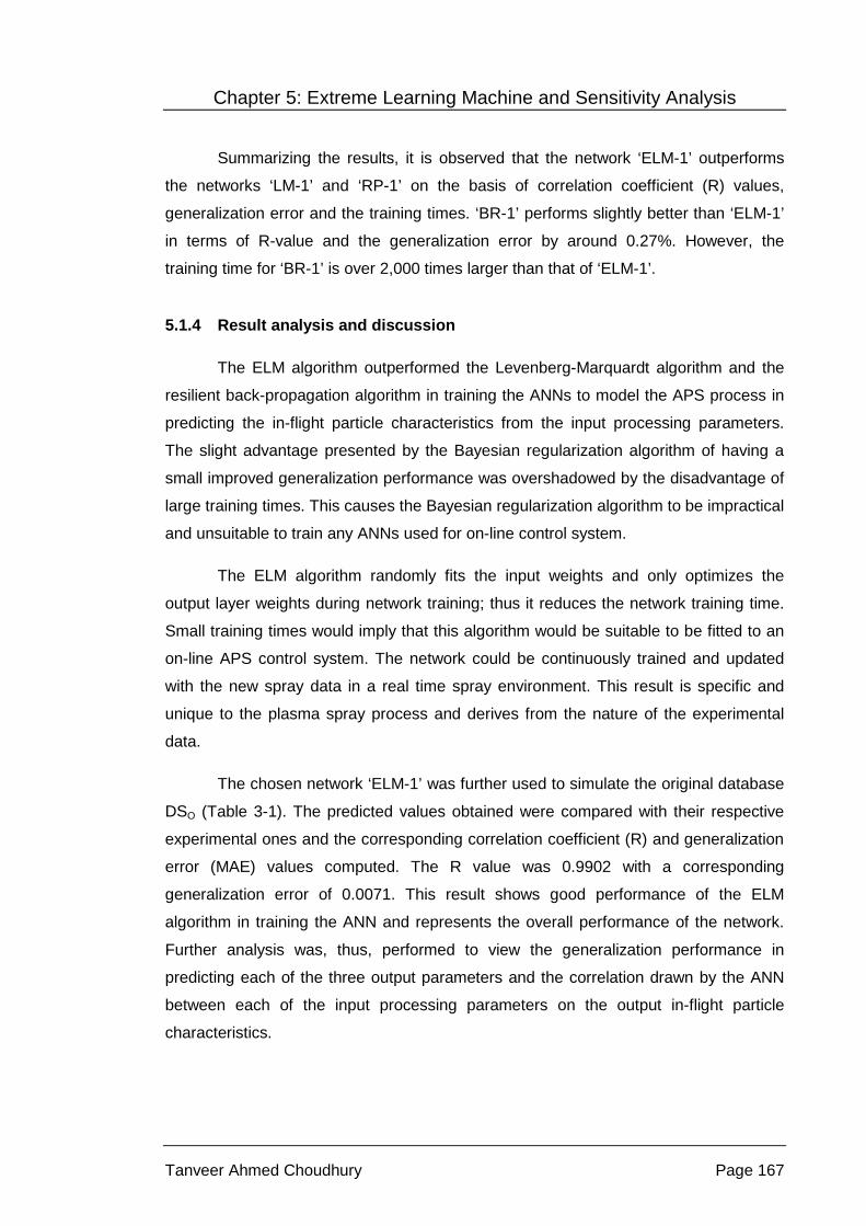
Chapter 5: Extreme Learning Machine and Sensitivity Analysis
Tanveer Ahmed Choudhury Page 167
Summarizing the results, it is observed that the network ‘ELM-1’ outperforms
the networks ‘LM-1’ and ‘RP-1’ on the basis of correlation coefficient (R) values,
generalization error and the training times. ‘BR-1’ performs slightly better than ‘ELM-1’
in terms of R-value and the generalization error by around 0.27%. However, the
training time for ‘BR-1’ is over 2,000 times larger than that of ‘ELM-1’.
5.1.4 Result analysis and discussion
The ELM algorithm outperformed the Levenberg-Marquardt algorithm and the
resilient back-propagation algorithm in training the ANNs to model the APS process in
predicting the in-flight particle characteristics from the input processing parameters.
The slight advantage presented by the Bayesian regularization algorithm of having a
small improved generalization performance was overshadowed by the disadvantage of
large training times. This causes the Bayesian regularization algorithm to be impractical
and unsuitable to train any ANNs used for on-line control system.
The ELM algorithm randomly fits the input weights and only optimizes the
output layer weights during network training; thus it reduces the network training time.
Small training times would imply that this algorithm would be suitable to be fitted to an
on-line APS control system. The network could be continuously trained and updated
with the new spray data in a real time spray environment. This result is specific and
unique to the plasma spray process and derives from the nature of the experimental
data.
The chosen network ‘ELM-1’ was further used to simulate the original database
DSO (Table 3-1). The predicted values obtained were compared with their respective
experimental ones and the corresponding correlation coefficient (R) and generalization
error (MAE) values computed. The R value was 0.9902 with a corresponding
generalization error of 0.0071. This result shows good performance of the ELM
algorithm in training the ANN and represents the overall performance of the network.
Further analysis was, thus, performed to view the generalization performance in
predicting each of the three output parameters and the correlation drawn by the ANN
between each of the input processing parameters on the output in-flight particle
characteristics.

Chapter 5: Extreme Learning Machine and Sensitivity Analysis
Tanveer Ahmed Choudhury Page 168
The absolute relative error percentage (with respect to the experimental values)
was computed for each value of the predicted in-flight particle characteristics, Table
5-3. The absolute average relative error percentages for in-flight particle velocity,
temperature and diameter were computed to be 1.60%, 0.52% and 0.63%,
respectively. The predicted velocity, temperature and diameter values by the network
‘ELM-1’ demonstrate good coherence and correlation with the experimental values.
The order of magnitude in errors obtained is well within the experimental errors of
these physical measurements; implying that the methods adopted with the ELM
algorithm are acceptable. All the predicted values were obtained from analysis of the
original database and represent the existing correlations.

Chapter 5: Extreme Learning Machine and Sensitivity Analysis
Tanveer Ahmed Choudhury Page 169
Table 5-3: Input processing parameters along with the corresponding experimental and
predicted in-flight particle characteristics values. The individual and average absolute
relative error percentage is also mentioned. Note: the variations of each of the input
processing parameters are highlighted in bold. The other parameter values were hold
constant to their reference values.
I [A]
VAr [SLPM]
VH2 [SLPM]
VCG [SLPM]
Dinj [mm]
ID [mm] * V
[m/s] T
[°C] D
[μm]
350 40 14 3.2 6 1.8 E 242 2262 43 P 241.58 2261.11 42.91
RE 0.17 0.04 0.22
530 40 14 3.2 6 1.8 E 270 2399 51 P 264.84 2378.00 49.96
RE 1.91 0.88 2.04
750 40 14 3.2 6 1.8 E 278 2428 50 P 277.71 2427.66 49.93
RE 0.10 0.01 0.14
530 40 0 3.2 6 1.8 E 205 1675 30 P 206.41 1721.15 30.16
RE 0.69 2.76 0.54
530 40 4 3.2 6 1.8 E 241 2170 38 P 239.66 2140.52 37.74
RE 0.56 1.36 0.69
530 40 8 3.2 6 1.8 E 260 2351 45 P 260.28 2356.58 45.16
RE 0.11 0.24 0.36
530 40 10 3.2 6 1.8 E 264 2373 47 P 265.30 2397.93 47.94
RE 0.49 1.05 1.99
530 45 15 3.2 6 1.8 E 176 2403 51 P 194.53 2390.26 50.58
RE 10.53 0.53 0.83
530 22.5 7.5 3.2 6 1.8 E 179 2456 49 P 180.49 2451.50 48.94
RE 0.83 0.18 0.13
530 37.5 12.5 3.2 6 1.8 E 263 2393 50 P 287.43 2395.75 49.51
RE 9.29 0.11 0.97
530 40 14 2.2 6 1.8 E 252 2352 48 P 251.61 2351.77 47.97
RE 0.15 0.01 0.06
530 40 14 4.4 6 1.8 E 277 2440 54 P 277.01 2438.78 53.90
RE 0.00 0.05 0.18
530 40 14 3.2 7 1.8 E 270 2434 47 P 271.76 2461.39 47.85
RE 0.65 1.13 1.81
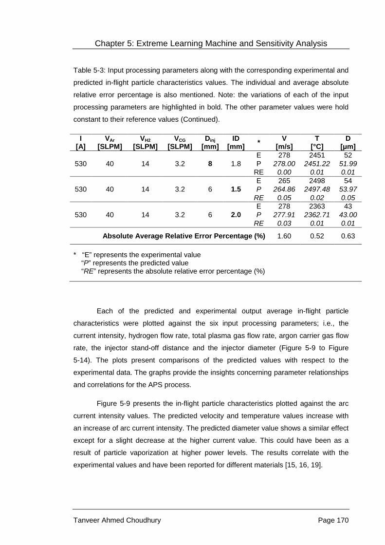
Chapter 5: Extreme Learning Machine and Sensitivity Analysis
Tanveer Ahmed Choudhury Page 170
Table 5-3: Input processing parameters along with the corresponding experimental and
predicted in-flight particle characteristics values. The individual and average absolute
relative error percentage is also mentioned. Note: the variations of each of the input
processing parameters are highlighted in bold. The other parameter values were hold
constant to their reference values (Continued).
I [A]
VAr [SLPM]
VH2 [SLPM]
VCG [SLPM]
Dinj [mm]
ID [mm] * V
[m/s] T
[°C] D
[μm]
530 40 14 3.2 8 1.8 E 278 2451 52 P 278.00 2451.22 51.99
RE 0.00 0.01 0.01
530 40 14 3.2 6 1.5 E 265 2498 54 P 264.86 2497.48 53.97
RE 0.05 0.02 0.05
530 40 14 3.2 6 2.0 E 278 2363 43 P 277.91 2362.71 43.00
RE 0.03 0.01 0.01
Absolute Average Relative Error Percentage (%) 1.60 0.52 0.63
* “E” represents the experimental value “P” represents the predicted value “RE” represents the absolute relative error percentage (%)
Each of the predicted and experimental output average in-flight particle
characteristics were plotted against the six input processing parameters; i.e., the
current intensity, hydrogen flow rate, total plasma gas flow rate, argon carrier gas flow
rate, the injector stand-off distance and the injector diameter (Figure 5-9 to Figure
5-14). The plots present comparisons of the predicted values with respect to the
experimental data. The graphs provide the insights concerning parameter relationships
and correlations for the APS process.
Figure 5-9 presents the in-flight particle characteristics plotted against the arc
current intensity values. The predicted velocity and temperature values increase with
an increase of arc current intensity. The predicted diameter value shows a similar effect
except for a slight decrease at the higher current value. This could have been as a
result of particle vaporization at higher power levels. The results correlate with the
experimental values and have been reported for different materials [15, 16, 19].
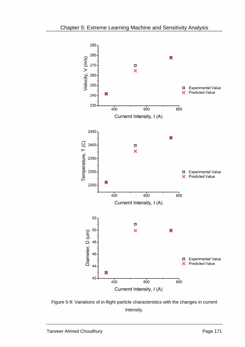
Chapter 5: Extreme Learning Machine and Sensitivity Analysis
Tanveer Ahmed Choudhury Page 171
Figure 5-9: Variations of in-flight particle characteristics with the changes in current
intensity.

Chapter 5: Extreme Learning Machine and Sensitivity Analysis
Tanveer Ahmed Choudhury Page 172
The predicted values of the in-flight particle characteristics follow the
experimental values in presenting a rising trend with an increase of the hydrogen
secondary plasma gas flow rate; Figure 5-10. The hydrogen content in the plasma gas
improves the velocity, temperature and enthalpy of the plasma jet [158] along with the
heat and momentum transfer to the particles [159]. These conditions improve the
overall in-flight particle characteristics [160, 161].
From Figure 5-11, the predicted in-flight particle velocity increases with an
increase of the total plasma gas flow rate. The predicted particle temperature is, on the
other hand, found to drop initially and then rise rapidly. The results correlate with the
experimental values. However, these results partially contradict the findings reported in
the literature [161].The finding indicates an increase in both the velocity and
temperature with an increase of the total plasma gas flow rate. From 30 SLPM (Run 9:
Table 3-1) to 40 SLPM (Run 4: Table 3-1), the hydrogen secondary plasma gas flow
rate is nearly doubled, while the argon primary plasma gas flow rate is made 0. This is
directly related to the increase of the momentum being transmitted from the plasma jet
to the particles, which leads to a decrease in the particle residence time in the plasma
jet. This could result in a drop in particle temperature. The predicted diameter values
correlate with the trend presented by the experimental values.
The VAr and VH2 values of 45 and 15 SLPM (Run 8: Table 3-1) were not
considered because the VAr value was greater than its highest individual limit.
Therefore, bias would be introduced into the experimental values since Run 8 is well
out of the range of conventional thermal spray processing parameters. Thus, this value
has not been considered in the analysis since the observations drawn for the whole
data set would be considered inconclusive.

Chapter 5: Extreme Learning Machine and Sensitivity Analysis
Tanveer Ahmed Choudhury Page 173
Figure 5-10: Variations of in-flight particle characteristics with the changes in hydrogen
plasma gas flow rate.

Chapter 5: Extreme Learning Machine and Sensitivity Analysis
Tanveer Ahmed Choudhury Page 174
Figure 5-11: Variations of in-flight particle characteristics with the changes in total
plasma gas flow rate.

Chapter 5: Extreme Learning Machine and Sensitivity Analysis
Tanveer Ahmed Choudhury Page 175
An increase in the carrier gas flow improves particle penetration into the core of
the plasma jet [1, 62]. This results in an increase of the in-flight particle characteristics.
The predicted values correlate to both the experimental database and the findings in
the literature (Figure 5-12).
Variations of injector stand-off distance and injector diameter influence particle
penetration into the plasma jet [62]. An increase in the injector stand-off distance
should improve the particle characteristics. On the other hand, an increase in the
injector diameter should lower the in-flight particle characteristic value.
Figure 5-13 presents an improvement of all the predicted values of the in-flight
particle characteristics with the increase of injector stand-off distance. This finding
correlates with the experimental values as well as those from the literature. Figure 5-14
shows the predicted in-flight particle values, along with the experimental values,
against the change in injector diameter. The experimental and simulation results are,
however, controversial to analyse. The experimental velocity and diameter values
indicate an increase with the injector diameter values, whereas the temperature
decreases. The predicted values are in complete coherence, both in terms of values
and trends, to the experimental values.
The above analysis helps in understanding the effects of variations of input
processing parameters on the output in-flight particle characteristics of the plasma
spray process. It further demonstrates the ability of the ELM algorithm to train an ANN
in modelling the APS process and learn the underlying relationships between the input
and output parameters. The ELM algorithm was used to train the networks using the
expanded database. The trained networks, when tested with the original database,
performed well. This indicates similarity of the information contained in the expanded
dataset and the original dataset.

Chapter 5: Extreme Learning Machine and Sensitivity Analysis
Tanveer Ahmed Choudhury Page 176
Figure 5-12: Variations of in-flight particle characteristics with the changes in carrier
gas flow rate.

Chapter 5: Extreme Learning Machine and Sensitivity Analysis
Tanveer Ahmed Choudhury Page 177
Figure 5-13: Variations of in-flight particle characteristics with the changes in injector
stand-off distance.

Chapter 5: Extreme Learning Machine and Sensitivity Analysis
Tanveer Ahmed Choudhury Page 178
Figure 5-14: Variations of in-flight particle characteristics with the changes in injector
diameter.

Chapter 5: Extreme Learning Machine and Sensitivity Analysis
Tanveer Ahmed Choudhury Page 179
5.1.5 Summary
SLFNs were used in this work to model the APS process in predicting the in-
flight particle characteristics from the input processing parameters. The ELM algorithm
used to train the SLFNs was successful in modelling the process dynamics. The ELM
algorithm showed better performance than most of the standard back propagation
algorithms used to train multi-layer feed forward networks. Simulation results confirm
the better performance of ELM both in terms of good generalization ability and shorter
training times.
Furthermore, the generalization performance of the ELM algorithm, over various
networks with different combinations of the number of hidden layer neurons, was more
stable than the back propagation algorithms. These features depict the stability and
robustness of the network learning process. The network stability, robustness and
significantly reduced training times of ELM makes it a desirable candidate to be
incorporated to an on-line plasma spray control system. Such a system would benefit
the plasma spray manufacturing process and assist spray engineers in reducing the
time and complexities associated with spray tuning and setting the crucial thermal
spray parameters.
5.2 Sensitivity analysis of neural networks
5.2.1 Background
In a real time spray process there are variations of the input processing
parameters over time. These variations affect the in-flight particle characteristics and it
is important to know the response of these fluctuations by the designed ANN model.
The network with good generalization ability is not expected to be responsive to the
slight variations of the input processing parameters. The network should only respond if
the variations exceed a specified limit. The limit could be pre-determined before the
start of the spray process.
Most of the variations of input processing parameters result from mechanical
disturbances and can be considered as noise for ANN modelling purposes. The model
is expected to show a certain degree of robustness in compensating for noise. This

Chapter 5: Extreme Learning Machine and Sensitivity Analysis
Tanveer Ahmed Choudhury Page 180
would enhance the reliability of the designed ANN model being incorporated to an on-
line plasma spray system.
Assuming the input parameters to remain constant during a real time spray
environment, disturbances can occur with the network parameters; namely the weights
and biases. These disturbances are important and affect the network output in-flight
particle characteristics. However, the artificial neural network models, proposed for an
on-line control system are generally in the form of a computer program and without
hardware implementation. The probability of the network parameters fluctuating are,
thus, low and can be ignored. Hence, this study only considers the effects of the
fluctuations of the input processing parameters on the designed ANN models in
predicting the output in-flight particle characteristics.
Uniform distributed noise is generated in this study to simulate the effect of
input parameter disturbances. The noises are gradually added to the model inputs to
simulate their effects on the outputs of the trained ANNs. The response of various
networks to different levels of noise were computed and compared with the original
output in-flight particle characteristics. The correlation coefficient (R) values were
computed and the results were analysed to find the degree of fluctuation. Figure 5-15
provides a flowchart to illustrate the work described in this section.
This study uses both MLP and SLFN structures to observe the effects of input
noises on the model output in-flight particle characteristics. Error BP algorithms are
used to train both the MLPs and SLFNs. The ELM algorithm is used in this work to train
the SLFNs. Sensitivity and robustness of the different networks are compared and
analysed, in terms of handling input noise.
Section 5.2.2 introduces to the database handling and noise generation and
addition process. Section 5.2.3 introduces the different ANN models used in this
section to carry out the noise sensitivity analysis. The details of simulation results,
analysis and discussions are presented in Section 5.2.4 with a summary in Section
5.2.5.

Chapter 5: Extreme Learning Machine and Sensitivity Analysis
Tanveer Ahmed Choudhury Page 181
Figure 5-15: Flowchart of the sensitivity analysis of designed artificial neural network
models to the fluctuations of the atmospheric plasma spray input processing
parameters.
5.2.2 Database processing and noise addition
The unexpanded original database, DSO (Table 3-1), was used in this section
as the test set for simulating the effects of noise on different, already developed, ANNs.
The database contained 16 data points and was linearly transformed within values of 0
and 1 using Equation 3-1. The normalization ensures equal treatment from ANN in
handling and processing the data. It also prevents any calculation error related to
different parameter magnitudes.
The MATLAB Simulink uniform noise generator block was used to generate the
uniformly distributed noise. The disturbances to the APS input processing parameters
generally occur within a small permissible range. The noise generated should also be
within a small range of values to correlate such affects. The uniform noise generator
was used in this work as the block allows pre-defining of both the upper and lower
bound of the noise values. The absolute upper limit value was set to 0.25, while the

Chapter 5: Extreme Learning Machine and Sensitivity Analysis
Tanveer Ahmed Choudhury Page 182
absolute lower limit value was set to -0.25. The defined limits allowed generation of
both positive and negative noise values. The positive value noises were used to
simulate the increasing effects of the input processing parameters. The negative values
represented the parameters decreasing effects.
Out of the six APS input processing parameters, the injector diameter and
injector stand-off distance have discrete values and are highly unlikely to be affected by
any disturbances. Therefore, the noise was only added to the remaining four input
parameters, namely: (i) arc current intensity, (ii) argon gas flow rate, (iii) hydrogen gas
flow rate, and (iv) argon carrier gas flow rate. Separate sets of uniform noise were
generated for each of the input processing parameters.
The noise generated by MATLAB represents normalized values. Equation 3-1
was used to format the normalized values to real parameter values. Taking the
example of current intensity, the normalized uniformly distributed noise generated by
MATLAB Simulink block was within the upper and lower limit of -0.2453 to 0.2396.
Using Equation 3-1, the corresponding real parameter values are -131.88 A to
128.82A. Table 5-4 provides the maximum and minimum values of the range of
uniformly distributed noise generated for each input process parameter. Both the
normalized and real parameter values are presented.
Table 5-4: Upper and lower limits of the uniform distributed noise values generated for
each of the input atmospheric plasma spray input processing parameters.
Input Processing Parameters
Uniform Distributed Noise Limits
Normalized Values Real Parameter Values Upper Limit
Lower Limit
Upper Limit
Lower Limit
Current Intensity I [A] 0.2396 -0.2453 128.82 -131.88
Argon Gas Flow Rate ArV [SLPM] 0.2255 -0.2412 5.41 -5.79
Hydrogen Gas Flow Rate
2HV [SLPM] 0.2493 -0.2482 4.24 -4.22
Argon Carrier Gas Flow Rate CGV [SLPM] 0.2127 -0.2393 0.64 -0.72

Chapter 5: Extreme Learning Machine and Sensitivity Analysis
Tanveer Ahmed Choudhury Page 183
5.2.3 Artificial neural network models
The effects of input parameter noise were tested on the ANN models proposed
and developed from Chapter 3, Chapter 4 and Section 5.1 of Chapter 5. The previously
selected models, in terms of generating the maximum correlation coefficient (R) values
from each section, were chosen for this purpose. The networks chosen were NN1,
NN2, 111-M, NET-C and ELM-1. A brief introduction and review of how each of these
networks was obtained are illustrated in the following paragraphs.
Chapter 3 used a general MLP ANN structure for modelling the APS to predict
the in-flight particle characteristics from the input power and injection parameters. The
Levenberg-Marquardt and Bayesian regularization back propagation algorithms were
used for network training purpose.
Figure 3-6 and Table 3-4 presented the generalization performance of the
networks trained with the Levenberg-Marquardt algorithm using both the unexpanded
training dataset, DSOTR, and the expanded training dataset, DSETR. The Section 3.5
compared the generalization performances of the different network models. The
analysis highlights the network with a combination of nine and eight neurons in the first
and second hidden layer, respectively, to generate the lowest generalization error of
2.00x10⁻⁵ and corresponding R-value of 0.9988. This network was referred to as NN1.
Figure 3-9 presented the accumulated results for all the networks trained with
the expanded training dataset, DSETR using a Bayesian regularization algorithm.
Section 3.5 presents the performance comparison of all such trained networks. The
network, with a combination of eight and seven neurons in the first and second hidden
layers, generated the maximum R-value of 0.9996 with a corresponding minimum
generalization error of 7.79x10⁻⁶. This network was referred to as NN2.
Section 4.1 proposed and used an optimized MLP structure ‘111’ to model the
APS process in predicting the output in-flight particle characteristics from the input
processing parameters. Figure 4-3 in Section 4.1.5.1 presented the bar chart
comparison of R-values and generalization errors of all the networks with structure
‘111’ and having different combinations of neurons in the hidden layers. All the
networks were trained with the Levenberg-Marquardt algorithm with the expanded
training dataset, DSETR. The network with 8 and 7 neurons, in the 1st and 2nd hidden
layers respectively, was marked as ‘111-M’. This network generated the maximum

Chapter 5: Extreme Learning Machine and Sensitivity Analysis
Tanveer Ahmed Choudhury Page 184
correlation (an R-value of 0.9996) between the predicted and actual outputs, when
simulated with the test set.
Section 4.2 used a modular ANN method to model the APS process. The
method allowed ANN to individually correlate each of the three output in-flight particle
characteristics with the APS input processing parameters. The APS process was, thus,
split into three sub-processes and each sub-process was assigned a different ANN,
termed as NET1, NET2 and NET3. NET1 was used to model the in-flight particle
velocity with the APS input parameters. NET2 and NET3 were used for modelling the
in-flight temperature and diameter, respectively, with the selected APS parameters.
The process is illustrated in Section 4.2.2. The database obtained from the literature
and presented in Table 3-1 was split up accordingly and was used for network training
and testing purposes, Section 4.2.3. A Bayesian regularization algorithm was used for
network training, Section 4.2.4.
Section 4.2.6 presents the simulation results for modular ANN implementation
of the APS process along with detailed comparison, analysis and discussion. From
Section 4.2.6.3, it was found that NET1 achieved the highest R-value of 0.8665, for
predicting the in-flight particle velocity, with 23 hidden layer neurons. This network was
named as NET1-M. NET2 predicted the average in-flight particle temperature with a
maximum R-value of 0.9999 with 3 hidden layer neurons. The network was named as
NET2-M. NET3 required 2 hidden layer neurons to achieve the highest R value of
0.9896 in predicting the in-flight particle diameter and was named as NET3-M. The
outputs of NET1-M, NET2-M and NET3-M were combined, using the Figure 4-14
structure, to generate the final model outputs, labelled as NET-C. NET-C generated the
R-value of 0.8317, Section 4.2.6.3.
Section 5.1 used a single layer feed forward neural network (SLFN) structure to
model the APS process in predicting the output in-flight particle characteristics from the
input power and injection processing parameters. A fast extreme learning machine
(ELM) algorithm was used to train the ANNs. The expanded training dataset DSETR was
used for network training. The generalization performances of the trained networks
were obtained by testing the trained networks with the expanded test dataset DSET.
Section 5.1.2 illustrates the database handling steps, while Section 5.1.2.2 elaborates
the network training conditions.

Chapter 5: Extreme Learning Machine and Sensitivity Analysis
Tanveer Ahmed Choudhury Page 185
Section 5.1.3.1 presented the performance of the ELM algorithm in training the
ANNs in correlating the input / output parameter relationships. Figure 5-2 presents the
variations of correlation coefficient (R) and generalization error (MAE) values with the
changes in the number of hidden layer neurons. The maximum R-value obtained was
0.9950 with 242 hidden layer neurons. This network named as ‘ELM-1’. The minimum
error of 0.0070 was found for the network ‘ELM-1’ with 242 hidden layer neurons.
5.2.4 Simulation result analysis and discussion
The generated noise was gradually added to the specified input parameters of
DSO. The amount of noise added was varied from zero to one hundred percent, with
increments of one percent. The selected networks NN1, NN2, 111-M, NET-C and ELM-
1 were simulated with the noisy database by the incremental addition of a percent of
noise. The correlation coefficient (R) value was computed for the resultant network
outputs with respect to the outputs from DSO. The R-value provides an understanding
of the degree of deviation of the network outputs from the expected values. Smaller R-
value depicts greater deviation of the predicted values from the original outputs in DSO.
The R-value, generated by the selected networks, with zero percent noise
represents the ideal condition; the condition under which the networks were modelled,
trained and tested. This value is termed as R0. The variations of the R-values for each
of the networks with the gradual addition of the noise are observed. The trend provides
a good understanding of how each of the artificial neural networks, trained with
different algorithms, network structures and training conditions, respond to fluctuations
of the input parameters. Figure 5-16 to Figure 5-20 provides graphs for the change of
R-values for each of the selected networks with the increase of the noise percentage
on the input test data.
For the network NN1 in Figure 5-16, the correlation coefficient dropped from its
maximum value of R0=0.9154 to 0.3149 with one hundred percentage addition of input
noises. Apart from the slight flattening in the 30 to 50 percent noise range, the drop in
correlation coefficient value was steady. The total drop of R-value was computed to be
0.6005 (Total drop of R = R0 – Rmin = 0.9154 - 0.3149 = 0.6005).
Chapter 5: Extreme Learning Machine and Sensitivity Analysis
Tanveer Ahmed Choudhury Page 186
Figure 5-16: Variations of correlation coefficient (R) values of the selected network NN1
output in-flight particle characteristics with the gradual addition of noise to the
atmospheric plasma spray specified input processing parameters.

Chapter 5: Extreme Learning Machine and Sensitivity Analysis
Tanveer Ahmed Choudhury Page 187
In comparison to the performance of NN1 in Figure 5-16, the performance of
NN2, as shown in Figure 5-17, was irregular and noisy. With the addition of only one
percent noise, the R dropped from its maximum value of 0.9996 to 0.5732. The value
dropped down rapidly to around 0.3. The R-value fluctuated around 0.3 until the input
disturbance reached around 25 percent, after which there was again a sudden drop.
The minimum R-value achieved was -0.0690 for the input noise percentage of 52
percent.
Figure 5-17: Variations of correlation coefficient (R) values of the selected network NN2
output in-flight particle characteristics with the gradual addition of noise to the
atmospheric plasma spray specified input processing parameters.

Chapter 5: Extreme Learning Machine and Sensitivity Analysis
Tanveer Ahmed Choudhury Page 188
For the network 111-M in Figure 5-18, there was an exponential decay of the R-
value, from R0 (0.9993) to the minimum value of -0.0158, with the gradual increase of
the input noise percentage.
Figure 5-18: Variations of correlation coefficient (R) values of the selected network 111-
M output in-flight particle characteristics with the gradual addition of noise to the
atmospheric plasma spray specified input processing parameters.

Chapter 5: Extreme Learning Machine and Sensitivity Analysis
Tanveer Ahmed Choudhury Page 189
Correlating to Figure 5-18, the R-values for the networks, NET-C and ELM-1 in
Figure 5-19 and Figure 5-20, respectively, also decreases with the increase of noise
percentage. However, the rate of decay is much lower and the decay trend is not
exponential.
Figure 5-19: Variations of correlation coefficient (R) values of the selected network
NET-C output in-flight particle characteristics with the gradual addition of noise to the
atmospheric plasma spray specified input processing parameters.

Chapter 5: Extreme Learning Machine and Sensitivity Analysis
Tanveer Ahmed Choudhury Page 190
Figure 5-20: Variations of correlation coefficient (R) values of the selected network
ELM-1 output in-flight particle characteristics with the gradual addition of noise to the
atmospheric plasma spray specified input processing parameters.
Figure 5-21 plots the variations of R-values with the input noise percentage, for
all the selected networks, in a single graph for better understanding and comparison
purpose. In all the cases, the values of R were reduced with the addition of noise
percentage. The networks output became more scattered with the increase of input
data noise. However, there were variations in which the networks responded. Some of
the networks were found to be less responsive to the noise addition and some
networks were sensitive to small percentage of input disturbances. Additional analyses
are carried out and the descriptions of the nature of responses of each network are
described in following paragraphs.
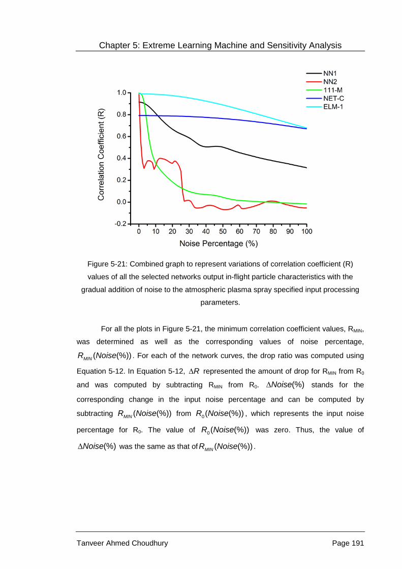
Chapter 5: Extreme Learning Machine and Sensitivity Analysis
Tanveer Ahmed Choudhury Page 191
Figure 5-21: Combined graph to represent variations of correlation coefficient (R)
values of all the selected networks output in-flight particle characteristics with the
gradual addition of noise to the atmospheric plasma spray specified input processing
parameters.
For all the plots in Figure 5-21, the minimum correlation coefficient values, RMIN,
was determined as well as the corresponding values of noise percentage,
( (%))MINR Noise . For each of the network curves, the drop ratio was computed using
Equation 5-12. In Equation 5-12, R∆ represented the amount of drop for RMIN from R0
and was computed by subtracting RMIN from R0. (%)Noise∆ stands for the
corresponding change in the input noise percentage and can be computed by
subtracting ( (%))MINR Noise from 0( (%))R Noise , which represents the input noise
percentage for R0. The value of 0( (%))R Noise was zero. Thus, the value of
(%)Noise∆ was the same as that of ( (%))MINR Noise .

Chapter 5: Extreme Learning Machine and Sensitivity Analysis
Tanveer Ahmed Choudhury Page 192
0
0
0
MIN
MIN
MIN
MIN
RDrop RatioNoise(%)
R R R (Noise(%))-R (Noise(%))
R R R (Noise(%))
∆=∆
−=
−=
Equation 5-12
The drop ratio value provides an understanding of the ANN sensitivity to the
variations of the input parameters. A higher drop ratio would indicate larger changes in
the correlation coefficient values in comparison to the changes in input noise
percentages. This would show that the network is more sensitive to the fluctuations of
input parameters. On the other hand, a lower value of the drop ratio results from small
change in the correlation coefficient values in relation to the changes in the amount of
input noise percentage. This would represent a network more rigid to the input
parameter fluctuations.
The bar chart representing the drop ratios for all the five selected networks is
presented in Figure 5-22. NET-C exhibited the least drop ratio of 0.0012 among all the
networks. This indicates that the performance of the modular ANNs is least sensitive to
the additions of input parameter disturbances. The result is in coherence to that of
Figure 5-21. The change in R-value, from zero to one hundred percent noise addition,
is small. The plot, represented by the deep blue line, is flatter in comparison to the
graphs for other networks.
The network NN2 revealed the highest drop ratio of 0.0206, Figure 5-22. The
result coincides with the plot obtained in Figure 5-21. The network NN2 was sensitive
to small variations of the input parameters. The R-value of the output from the
simulated noisy input dropped rapidly, represented by the red line. The next in line, in
terms of the networks sensitivity to the input parameters, is the network 111-M. The
magnitude of the drop in R-value was close to that of NN2. However, the trend was
smoother and less rapid. This is represented by a lower drop ratio of 0.0102.
The sensitivity of the networks ELM-1 and NN1 to the variations of the input
parameters was moderate. The ELM-1 and NN1 generates the drop ratio values of
0.0031 and 0.0060, respectively, Figure 5-22. The drop in the R-value, with the
increase of the input noise percentage, in Figure 5-21 for the two networks is gradual

Chapter 5: Extreme Learning Machine and Sensitivity Analysis
Tanveer Ahmed Choudhury Page 193
but differs in the rate of decay. NN1 represents more exponential decay with higher
decay rate, while ELM-1 had a lower decay rate.
Figure 5-22: Drop ratios for selected artificial neural networks.
Table 5-5 summarizes and tabulates the values of R0, RMIN, ( (%))MINR Noise ,
R∆ and the drop ratios for the five selected networks. In addition, the table provides
the percentage of noise, required to drop each of the networks’ R values to 95%, 90%,
85%, 80% and 75% of the R0 value. The results are extracted from Figure 5-21 and are
found to be in coherence with Figure 5-22. Network NN2 was the most sensitive of all
the networks; the R value dropped to lower than 95 percent of R0 with one percent of
noise added to the input parameters. NET-C was the least sensitive with sixty percent
of noise required to be incorporated to the input data to drop the network performance
to 95 percent of its R0.

Chapter 5: Extreme Learning Machine and Sensitivity Analysis
Tanveer Ahmed Choudhury Page 194
Table 5-5: Performance values for the sensitivity analysis of the different selected
networks with the fluctuations of the neural network input parameters.
NN1 NN2 111-M NET-C ELM-1
R0 0.9154 0.9996 0.9993 0.7916 0.9902
Minimum R-value (RMIN) 0.3149 -0.0690 -0.0158 0.6705 0.6789
Corresponding Noise Percentage (%)
MINR (Noise(%)) 100 52 100 100 100
ΔR 0.6005 1.0686 1.0151 0.1212 0.3115 Drop Ratio
ΔRΔNoise(%)
0.0060 0.0206 0.0102 0.0012 0.0031
Percentage of Noise (%)
NN1 NN2 111-M NET-C ELM-1
95% of R0 7 1 3 60 35
90% of R0 10 1 4 82 50
85% of R0 12 1 4 99 62
80% of R0 15 1 5 Greater than 100 74
75% of R0 19 1 5 Greater than 100 85
5.2.5 Summary
The sensitivity of an artificial neural network (ANN) is an important parameter to
study before incorporating the models to any on-line atmospheric plasma spray (APS)
control system. It is important to understand how the designed network model would
respond when conditions stray away from being ideal as the spray process proceeds.
The disturbances for an ANN can occur due to slight fluctuations of the input
parameters presented to the network or due to fluctuations of the network parameters
itself. The hardware implementation of the ANN models is not considered; therefore,
only the disturbances to the input parameters were considered.

Chapter 5: Extreme Learning Machine and Sensitivity Analysis
Tanveer Ahmed Choudhury Page 195
Different ANN models developed in the course of this research work were
considered for this analysis. The network models were trained and optimized under
different conditions, including different network structures, various training algorithms
and different training data sets.
The sensitivity of the selected networks to the fluctuations of the APS input
processing parameters were considered. Uniform distributed noise, generated by
MATLAB’s Simulink tool, was used in this study to simulate the effect of input
parameter disturbances. With the gradual addition of the noise to the input, the
networks were simulated and the correlation coefficient values (R) were computed to
show the changes in network’s performance.
For all the considered networks, the values of correlation coefficient were
reduced with the gradual addition of noise. The networks output became more
scattered with the increase of input data noise. However, there were variations in which
the networks responded. Some of the networks were found to be less responsive to the
noise addition; whereas some networks were sensitive to a small percentage of input
disturbances.
The network NN2, a MLP ANN structure trained with a Bayesian regularization
algorithm and an expanded training set, was the most sensitive to fluctuations of input
parameters. The modular network NET-C, a single hidden layer structure trained with
the original database and the Levenberg-Marquardt algorithm, was the least sensitive
to any changes in the input parameters.
Ranking the networks, in terms of highest sensitivity to the variations of the
input parameters to the lowest sensitivity, we obtain NN2, 111-M, NN1, ELM-1 and
NET-C. The ranking is based on the results obtained in Figure 5-21, Figure 5-22 and
Table 5-5. The study in this section would assist thermal spray engineers in selecting
appropriate artificial neural network models for any specific on-line plasma spray
control process based on individual system requirements.

Chapter 6 Experimental Work
And
Network Modelling

Chapter 6: Experimental Work and Network Modelling
Tanveer Ahmed Choudhury Page 197
Chapter 6 Experimental Work and Network Modelling
This chapter elaborates experiments carried out in relation to the atmospheric
plasma spray (APS) process. The input processing parameters were varied and the
changes in the dynamic behaviour of the in-flight particle characteristics were observed
using a dichromatic sensor. The processing parameters and corresponding in-flight
particle characteristic values were processed to form the experimental database. The
database was then used to train selected artificial neural network (ANN) structures and
models from previous chapters. The developed networks were found to successfully
model the APS process. The networks were able to learn the input / output parameter
relationships and correlate the in-flight particle characteristics with each of the input
processing parameters. The work, thus, provides validation of the proposed ANN
models and structures because the resultant ANNs were found to work both with the
new experimental data and a database from the literature. A flowchart outlining the
work done in this chapter is presented in Figure 6-1.
Figure 6-1: Research methodology for artificial neural network modelling of an
atmospheric plasma spray process with experimental dataset.

Chapter 6: Experimental Work and Network Modelling
Tanveer Ahmed Choudhury Page 198
Section 6.1 describes the APS experiment set-up and process parameter
selection. It explains the database collection and processing steps. Section 6.2
introduces the ANN models used in this work to model the APS process. The network
training, optimization and testing steps are illustrated in Section 6.3. Section 6.4
presents the simulation results and provides an analysis and discussion of the
performance of the ANN models on the experimental dataset. A summary of the results
obtained and the work done in the section is presented in Section 6.5.
6.1 Experiment design and plasma spray process set-up
The experiment was set-up to generate a thermal sprayed alumina-titania
(Al2O3-TiO2) coating, which is widely used in various industrial applications. In
comparison to the alumina-titania coatings, the pure alumina (Al2O3) coatings exhibit a
higher degree of hardness, erosion resistance and dielectric strength. However, the
coatings are brittle. A small amount of titania, blended with the alumina feedstock,
increases the toughness of the thermal spray coating. The 13 wt. % or 40 wt. % of
titania into an alumina feedstock generates a coating with higher toughness and lower
hardness, chemical resistance and electric resistivity. The Metco 131VF (Al2O3-
40 wt. % TiO2 -45+5 μm) power was used in the current experiment to form the coating.
The APS samples were created with the help of an industrial partner (United
Surface Technologies Pty. Ltd., Victoria – 3018, Australia). A Plasmadyne SG-100
system (Plasmadyne Corporation, USA) was used. The SG-100 plasma torch uses a
single cathode and anode configuration. The plasma jet is generated by primary
ionising argon gas. The enthalpy of the flame is increased using helium as the
secondary plasma gas. Helium is inferior as a secondary plasma gas in comparison to
an identical volume of hydrogen to improve the plasma jet enthalpy. However, helium
corrodes the electrodes less, thus, extending their lifetime.
The input processing parameters considered in the experiment were the (i) arc
current intensity, (ii) argon primary plasma gas flow rate, (iii) helium secondary plasma
flow rate, and (iv) argon carrier gas flow rate. The powder feed rate was set to 15 and
30 g/min with the substrate stand-off distance being 95 mm. The output in-flight particle
characteristics considered were the average in-flight particle (i) velocity, (ii)
temperature, and (iii) diameter. The input processing parameters were varied and the
corresponding output in-flight dynamic behaviour of the particles was measured using a

Chapter 6: Experimental Work and Network Modelling
Tanveer Ahmed Choudhury Page 199
dichromatic sensor (DPV – 2000 from TECNAR Automation Limited, St-Bruno, QC,
Canada J3V 6B5) from the centre of the particle flow stream.
The experimental values appear in Table 6-1 and form the experimental
database, EDSO. The database consisted of 14 data values. The in-flight particle
characteristics represent the average value over a fixed period of measurement from
the DPV-2000 sensor. The standard deviations of each of the in-flight particle velocity,
temperature and diameter, for each run of experiment, are noted in Table 6-2. The
powder feed rate and the substrate stand-off distance for each run of the experiment
are also presented in Table 6-2.
The variations of the input processing parameters in Table 6-1 are presented as
bold numbers. A single input processing parameter was varied at any time (Run 1 to
Run 13). The remaining parameters were fixed at their reference values. Run 14
consist of all the input processing parameters kept to their reference values. The
reference values of the input processing parameters are noted in the footnote of Table
6-1.
Chapter 3, Chapter 4 and Chapter 5 used the database DSO (Table 3-1) from
literature [40] for ANN modelling of the APS process. A critical difference between DSO
and the experimental, EDSO, is in the number of input parameters considered. The
database, DSO, from the literature used six input parameters: (i) arc current intensity,
(ii) primary plasma gas flow rate, (iii) secondary plasma flow rate (iv) carrier gas flow
rate, (v) injector diameter, and (vi) injector stand-off distance. The experimental
database, EDSO, however, considered only the first four input processing parameters
for variation. The reasoning is as follows.
The work described in the literature [40] employed a Sulzer-Metco F4 gun
(Wohlen, Switzerland) for spraying. The experiment carried out in this study, however,
used a different SG-100 torch. A key difference between the F4 plasma torch and the
SG-100 torch lies in the location of the powder port and the angle of powder injection.
In the SG-100 plasma torch, the powder port is incorporated into the anode assembly.
The angle of powder feed injection can be selected using different models of anode.
The angle of powder feed helps in the flow of powder particles into the plasma plume.
The experiment in this study deploys an anode (175 model) with an internal powder
feed at a 90° injection from horizontal axis. The use of SG-100 torch and experimental
setup fixed the parameters of injector diameter and injector stand-off distance. The

Chapter 6: Experimental Work and Network Modelling
Tanveer Ahmed Choudhury Page 200
experiment, therefore, considered and varied only the other four input processing
parameters.
Table 6-1: Experimental database (EDSO) consisting of the atmospheric plasma spray
input processing parameters and the output in-flight particle characteristics.
Run I [A]
ArV[l/min]
HeV[l/min]
CGV[l/min]
Experimental Values
V [m/s]
T [°C]
D [μm]
1 550 47.2 27.9 5.7 182 2355 23
2 650 47.2 27.9 5.7 194 2412 23
3 750 47.2 27.9 5.7 191 2450 21
4 650 40.1 27.9 5.7 170 2394 23
5 650 54.3 27.9 5.7 201 2381 21
6 650 47.2 24.1 5.7 185 2400 23
7 650 47.2 31.6 5.7 192 2416 22
8 650 47.2 27.9 5.2 213 2215 25
9 650 47.2 27.9 6.1 187 2182 26
10 650 47.2 27.9 6.1 197 2219 26
11 650 47.2 27.9 7.1 185 2375 21
12 650 47.2 27.9 7.1 219 2270 26
13 650 47.2 27.9 8.5 184 2360 20
14 650 47.2 27.9 5.7 201 2207 26
I Current Intensity (Reference value: 650 A)
ArV Argon primary plasma gas flow rate (Reference value: 47.2 l/min)
HeV Helium secondary plasma gas flow rate (Reference value: 27.9 l/min)
CGV Argon carrier gas flow rate (Reference value: 5.7 l/min)
V Average in-flight particle velocity
T Average in-flight particle temperature
D Average in-flight particle diameter

Chapter 6: Experimental Work and Network Modelling
Tanveer Ahmed Choudhury Page 201
Table 6-2: Atmospheric plasma spray process experiment parameters. The standard
deviations of the measured in-flight particle characteristics are indicated.
Run Feed Rate [g/min]
Substrate Stand-off Distance
SOD [mm]
Standard Deviations
Particle Velocity V [m/s]
Particle Temperature
T [°C]
Particle Diameter D [μm]
1 15 95 50 270 8
2 15 95 57 259 9
3 15 95 65 292 9
4 15 95 53 255 9
5 15 95 59 271 8
6 15 95 55 245 9
7 15 95 60 279 9
8 30 95 50 167 9
9 30 95 46 162 8
10 30 95 46 147 8
11 15 95 56 244 8
12 30 95 48 166 9
13 15 95 54 246 7
14 30 95 46 149 8
6.2 Artificial neural network modelling
The three artificial neural network models proposed and used in Chapter 3 and
Chapter 4 were used in this section for modelling the atmospheric plasma spray
process to predict the in-flight particle characteristics from the input processing
parameters. The experiment database, EDSO, with the error back-propagation
algorithm, was used for all the networks training and testing. A description of the
network structures is discussed in the following paragraphs.
The first ANN model is the two hidden layer multi-layer perceptron (MLP)
structure used in Chapter 3. For reference, all the networks trained with this structure,
in this section, are referred to as N1.

Chapter 6: Experimental Work and Network Modelling
Tanveer Ahmed Choudhury Page 202
The MLP structure used in Chapter 3 is presented in Figure 3-2. The chapter
used the database DSO (Table 3-1) from literature [40] for ANN modelling. As illustrated
in Section 6.1; the experimental database, EDSO, used in this chapter is different in
terms of the number of input processing parameters considered. EDSO contains only
four input processing parameters. Modification of the input layer of the MLP structure in
Figure 3-2 was, thus, necessary. The updated MLP architecture is presented in Figure
6-2.
Figure 6-2: Block diagram of the designed multi-layer artificial neural network (ANN)
structure.
As presented in Figure 6-2, the MLP architecture consists of three types of
layers; i.e., input layer, hidden layers and the output layer. The input layer is connected
to the input processing parameters and the output layer generates the network output,
which are the in-flight particle characteristics consisting of average particle velocity,
temperature and diameter. The layers in between the input and output layers are
named as the hidden layers. The hidden layer contains neurons to help the network
learn the input-output parameter relationships. The number of hidden layers is a
variable parameter. In correlating with the work in Chapter 3, the number of hidden
layers in this study was fixed to two, Figure 6-2.

Chapter 6: Experimental Work and Network Modelling
Tanveer Ahmed Choudhury Page 203
In Figure 6-2, jiw (where i = 1…4 and j = 1…N1) represents the input layer
weights. The terms jiα (where i = 1… N1 and j = 1… N2) and jiβ (where i = 1…N2 and
j=1…3) represent the hidden layer weights and output layer weights, respectively. N1
and N2 represent the number of neurons in hidden layer 1 and hidden layer 2;
respectively.
No generalized rule exists to specify the exact values of N1 and N2. A large
number of hidden layer neurons provide the network flexibility to optimize many
parameters and reach an improved solution. However, increasing the size of the
hidden layer over a certain limit makes the network under-characterized. The network
in such cases is forced to optimize more parameters than the data vectors available to
define these parameters. Too few a number of neurons in the hidden layers leads to
under-fitting. The performance of a trained ANN is sensitive to the number of hidden
layer neurons and the optimum number and combination of neurons in the hidden
layers are determined from the network training and optimization process.
The second model, used in this work, is based on the modified MLP ANN
architecture ‘111’ proposed and used in Section 4.1 of Chapter 4. These trained and
optimized networks are referred to as N2 in this section.
The default MLP ANN structure, presented in Figure 6-2, with two hidden
layers, consists of the input layer connected to the 1st hidden layer, which is connected
to the 2nd hidden layer. The 2nd hidden layer is then connected to the output layer. A
block diagram illustrating the structure is presented in Figure 4-1.
The network, with the proposed modified structure, is provided with additional
parameters to learn and generalize the process relationships without increasing the
number of hidden layer neurons. This is facilitated by modification of the layer
connection matrix. Additional connections were made from the input layer to the 2nd
hidden layer and also to the output layer. The MLP structure presented in Figure 6-2 is,
thus, modified as per the block diagram of the proposed structure in Figure 4-2.
The third and final network model used the modular ANN method implemented
in Section 4.2 of Chapter 4. The modular implementation allows simplification of the
designed ANN model in predicting the in-flight particle characteristics from the input
processing parameters of the APS process. The APS is first decomposed into sub-

Chapter 6: Experimental Work and Network Modelling
Tanveer Ahmed Choudhury Page 204
processes to simplify the problem the network is required to learn. Each sub-process is
a part of the whole APS process and is assigned a different ANN. Thus, each designed
ANN focuses on solving only a sub-process. The final solution is obtained by re-
combining the individual network solutions.
Decomposition of the task allowed simpler ANNs to be built and at the same
time helped the networks to learn the process better. The segmented approach allows
the user to understand the relationships that the model established between each of
the in-flight particle characteristics and the input processing parameters. The system
reliability is enhanced by splitting up the problem so that each network is trained to
solve a part of the whole problem. Any fault or error in prediction of one of the sub-
problems does not affect the entire solution to the problem.
With the existing knowledge and understanding of the APS process, explicit
decomposition was chosen for decomposition of the task into modular components.
The overall task in this work concentrated on predicting the three in-flight particle
characteristics (i.e., in-flight particle velocity, temperature and diameter) from the input
processing parameters of the APS process. The task was decomposed into three sub-
tasks, each considering the effects of input processing parameters on one of the in-
flight particle characteristics.
In this study, all the three output parameters were of equal importance. Co-
operative combination was used for the three modular components. The three outputs
from three modular components, each providing a solution to the sub-task assigned,
were combined with equal weighting to generate the final solution. A flowchart
illustrating the co-operative combination process, used in this study, is presented in
Figure 4-14.
All the APS input processing parameters in EDSO were fed into the input layer
of the networks. The first network (N3-V) generated the in-flight particle velocity at the
output layer, the second network (N3-T) generated the in-flight particle temperature
and the third network (N3-D) generated the in-flight particle temperature as the output.
Figure 6-3 provides a flowchart for the modular implementation of the APS process
used in this section.

Chapter 6: Experimental Work and Network Modelling
Tanveer Ahmed Choudhury Page 205
Figure 6-3: Flowchart for modular artificial neural network implementation of the
atmospheric plasma spray process.
The networks N3-V, N3-T and N3-D are based on single hidden layer fully
connected MLP model. The network architecture is presented in Figure 6-4. The single
hidden layer proved sufficient for the networks to learn the function defining the sub-
tasks assigned. The parameter jiw (where i = 1…4 and j = 1…N1) represents the
input layer weights. jiβ (where i = 1… N1 and j = 1) the output layer weights. The
parameter N1 defines the number of hidden layer neurons. The value is obtained
through network training and the optimization process.

Chapter 6: Experimental Work and Network Modelling
Tanveer Ahmed Choudhury Page 206
Figure 6-4: Single layer multi-layer perceptron (MLP) artificial neural network (ANN)
architecture.
For the purpose of training and testing the developed modular ANNs, the
database, EDSO (Table 6-1) was split into three sub-sets. The segmentation was based
on the three output parameters. Figure 6-5 provides a flow chart of the data split
process. The first subset, EDSO1, contained the input processing parameters and the
average in-flight particle velocity. The second subset, EDSO2, contained the input
processing parameters and the average in-flight particle temperature and the third
subset, EDSO3, contained the input processing parameters and the average in-flight
particle diameter.

Chapter 6: Experimental Work and Network Modelling
Tanveer Ahmed Choudhury Page 207
Figure 6-5: Flowchart representing the data split process for training of developed
modular artificial neural network models.
The flowchart depicting the overall research methodology presented in this
section is provided in Figure 6-6. The database, EDSO, was used for network training
and optimization of the networks, N1 and N2. The EDSO was split into EDSO1, EDSO2
and EDSO3 for training and testing of the modular ANNs N3-V, N3-T and N3-D. The
network outputs and performance of all the different networks were compared and
analysed.

Chapter 6: Experimental Work and Network Modelling
Tanveer Ahmed Choudhury Page 208
Figure 6-6: Research methodology for artificial neural network implementation of the
atmospheric plasma spray process to predict the output average of in-flight particle
characteristics using different artificial neural network models and structures.
6.3 Network training and optimization
The study considered supervised learning based on the BP algorithm. The
network size in this study is within a few hundred weights; therefore a non-linear least
squares numerical optimization method of the Levenberg-Marquardt (LM) algorithm

Chapter 6: Experimental Work and Network Modelling
Tanveer Ahmed Choudhury Page 209
(Section 2.2.2.2) was used for training all the considered networks N1, N2, N3-V, N3-T
and N3-D. The LM algorithm is considered more efficient in training than the conjugate
gradient method or the variable learning rate algorithm for a network with a few
hundred weights [100]. Other standard back propagation algorithms are slow and
require excessive off-line training. They also suffer from temporal instability and tend to
become fixed to the local minima [157].
The LM algorithm uses a standard statistical technique of cross-validation and
early stopping to combat the problem of over-fitting. The technique requires a separate
validation set to test whether the network has started to over-fit during the training. The
validation set is unseen to the network during its training. The error generated by the
networks on the validation sets provides a measure of the over-fitting. The network
training is stopped if the validation error starts to increase as the network is most likely
to have started over-fitting.
For the network N1 and N2, EDSO was split by interleaving in the ratio 0.80:0.20
to generate the training/validation dataset, EDSOTRV and test dataset EDSOT. The EDSO
contains 14 data values. The EDSOTRV and EDSOT, thus, contained 11 and 4 data
values, respectively. The EDSOTRV was used for the network training and validation
purpose while EDSOT was used only for network testing purposes. The dataset
EDSOTRV was further interleaved in the ratio 0.80:0.20 to generate the training dataset
EDSOTR (9 data values) and the validation dataset EDSOTV (2 data values).
For the modular networks, N3-V, N3-T and N3-D, the split databases EDSO1,
EDSO2 and EDSO3 were also interleaved in the ratio 0.80 to 0.20 to generate the
corresponding training/validation datasets (EDSO1TRV, EDSO2TRV and EDSO3TRV) and test
datasets (EDSO1T, EDSO2T and EDSO3T). The training/validation datasets were
interleaved in the same ratio of 0.80:0.20 to produce the individual training datasets
(EDSO1TR, EDSO2TR and EDSO3TR) and validation datasets (EDSO1V, EDSO2V and
EDSO3V). The entire data division processes are pictured in Figure 6-7. The number of
data values, for each dataset, is also noted.
The selected ratio 0.80:0.20 provides the optimal size of the training dataset for
the available database. A smaller training dataset would have reduced the networks
ability to learn the process dynamics. Increasing the number of training data points
would have reduced the size of the validation and test sets. The reduction in validation
set would have reduced the ability of the network to detect any over-fitting occurring

Chapter 6: Experimental Work and Network Modelling
Tanveer Ahmed Choudhury Page 210
during network training. Reduction in the size of the test set would have reduced the
test sets ability to test the trained networks generalization performance.
Figure 6-7: Data division process of the experimental database of the atmospheric
plasma spray process for training and testing of the different designed artificial neural
network models.
The LM is a fast algorithm in terms of the training speed. The training
parameters of the algorithm, when used together with early stopping, should be
adjusted to reduce the convergence speed. The parameter μ (Equation 2-44) was,

Chapter 6: Experimental Work and Network Modelling
Tanveer Ahmed Choudhury Page 211
thus, set to a relatively large value of 1. The μ increment parameter was set to 1.5,
while the μ decrement factor was set to 0.8. The number of training epochs was set to
300 and the maximum number of permitted validation error fails to 100. These limits
ensured that the network was allowed sufficient iterations to converge to the functions
global error minimum. The transfer function used in all layers was the log-sigmoid
function and the error performance function was set to the mean absolute error (MAE)
(Equation 3-7).
The training conditions were applied in training all the selected networks N1,
N2, N3-V, N3-T and N3-D with the Levenberg-Marquardt algorithm. In each case, the
network parameters were initialized to random values between 0 and 1.
The networks N1 and N2 were trained with the training dataset EDSOTR. The
trained networks were simulated with the test dataset, EDSOT. The computed R-values
on the test set indicated how well the trained networks responded to the unseen input
fits to their respective outputs. It provided a measure of the networks generalization
ability. The larger the average R-value, then better was the generalization performance
of the network and correlation between the predicted and actual values. The network
training was repeated one hundred times and the network generating the maximum R-
value of EDSOT was stored and saved. The training process was repeated as the
combination of the number of neurons in the 1st and 2nd hidden layer was varied from 2
and 1 to 20 and 19, respectively, with increments of one neuron in each hidden layer.
The modular networks N3-V, N3-T and N3-D were trained similarly with their
corresponding training datasets EDSO1TR, EDSO1TR and EDSO1TR, respectively. The
network training was repeated one hundred times. The networks generating the
maximum R-value on their respective test datasets were stored and saved each time.
The process was repeated with the number of hidden layer neurons varied from 1 to
20, with increments of one neuron.
6.4 Simulation result
6.4.1 Proposed network models
This sub-section elaborates the generalization performance of the trained
networks N1, N2, N3-V, N3-T and N3-D. The generalization performance includes the

Chapter 6: Experimental Work and Network Modelling
Tanveer Ahmed Choudhury Page 212
correlation coefficient, R, and generalization error values. The generalization error
represents the error generated by each network on their respective test dataset. As the
test set was unseen to the networks during the training process, the error generated
and correlation coefficient values generated by each of the networks provides an
understanding of the generalization performance of the networks.
Figure 6-8 plots the generalization performance of the networks N1. The figure
presents a bar chart comparison of R-values and generalization errors of all the
networks in N1 having different combinations of the number of neurons in the hidden
layers. The average R-value was 0.7756 with a maximum value of 0.9521 for a total of
only 9 neurons in the two hidden layers (5 and 4 neurons in the 1st and 2nd hidden layer
respectively). The average generalization error, of all the networks, was in the order of
0.1758. The network with 5 and 4 neurons, in the 1st and 2nd hidden layers respectively,
is marked as ‘N1-M’. This network was found to generate the maximum correlation (an
R-value of 0.9521) between the predicted and actual outputs, when simulated with the
test set.

Chapter 6: Experimental Work and Network Modelling
Tanveer Ahmed Choudhury Page 213
Figure 6-8: Generalization performances of all the artificial neural networks N1 with
different combination of the number of hidden layer neurons.
The network N2 generated an average correlation coefficient of 0.6971. The
average generalization error of all the networks was 0.2238. A bar chart comparison of
all the R-values and generalization errors of the networks in N2, with different
combinations of the number of neurons in the hidden layers, is presented in Figure 6-9.
The network with 19 and 18 neurons, in the 1st and 2nd hidden layers respectively,
Referenced as “N1-M” in the text

Chapter 6: Experimental Work and Network Modelling
Tanveer Ahmed Choudhury Page 214
generated the maximum correlation of 0.8137 on the test set. The network is named as
‘N2-M’.
Figure 6-9: Generalization performances of all the artificial neural networks N2 with
different combination of the number of hidden layer neurons.
Figure 6-10 provides a bar chart comparison of the R and generalization error
values of the designed modular ANN N3-V, trained with a different number of neurons
Referenced as “N2-M” in the text

Chapter 6: Experimental Work and Network Modelling
Tanveer Ahmed Choudhury Page 215
in the hidden layer. The average R-value, over all values of the hidden layers, was
0.9979 with the corresponding average generalization error of 0.1225. N3-V generated
the highest R-value of 0.9999 with 12 hidden layer neurons. The corresponding
generalization error was 0.1239. This network is marked as ‘N3-V-M’.
Figure 6-10: Generalization performances of the modular artificial neural network N3-V
with different combination of the number of hidden layer neurons.
Referenced as “N3-V-M” in the text

Chapter 6: Experimental Work and Network Modelling
Tanveer Ahmed Choudhury Page 216
Figure 6-11 provides a bar chart comparison of the generalization performances
of N3-T trained with a different number of neurons in the hidden layer. The average R
and generalization error values were computed to be 0.9283 and 0.1792, respectively.
For N3-T, the network with 8 hidden layer neurons generated the best performance in
terms of R-value over all the neuron numbers. The maximum R-value generated was
0.9999 with a corresponding generalization error of 0.1484. This network is referred to
as ‘N3-T-M’.
Figure 6-11: Generalization performances of the modular artificial neural network N3-T
with different combination of the number of hidden layer neurons.
Referenced as “N3-T-M” in the text

Chapter 6: Experimental Work and Network Modelling
Tanveer Ahmed Choudhury Page 217
Figure 6-12 provides a bar chart comparison of the correlation coefficient (R)
and generalization error values for N3-D trained with a different number of neurons in
the hidden layer. The average R-value and generalization error, over all the networks
trained, was 0.9897 and 0.1403, respectively. Among all networks in N3-D, the
network with just 6 hidden layer neurons generated the best generalization
performance with a maximum R value of 0.9999 and corresponding generalization
error of 0.1285. The network is marked as ‘N3-D-M’.
Figure 6-12: Generalization performances of the modular artificial neural network N3-D
with different combination of the number of hidden layer neurons.
Referenced as “N3-D-M” in the text

Chapter 6: Experimental Work and Network Modelling
Tanveer Ahmed Choudhury Page 218
6.4.2 Performance comparison and result analysis
The simulation results of the five selected networks N1, N2, N3-V, N3-T and
N3-D are compared and analysed further for better understanding the performance of
the proposed ANN models and structures in modelling the APS process.
The average generalization performances (average correlation coefficient (R)
values and average generalization errors) of all the selected networks are plotted as
bar graphs in Figure 6-13. The modular networks N3-V, N3-T and N3-D perform better
in comparison to the networks N1 and N2. The training dataset in this study was very
small. The dataset contained only 9 data values. In this case the modular methodology
allowed the networks to learn the APS input / output process relationships better. The
methodology simplified the problem by splitting the process and assigning separate
small single hidden layer ANNs to each sub-process.

Chapter 6: Experimental Work and Network Modelling
Tanveer Ahmed Choudhury Page 219
Figure 6-13: Average generalization performance comparison of different artificial
neural network models.
The generalization performances of the best performing networks marked in
Section 6.4.1 are compared and analysed in the following paragraphs. The marked
networks are N1-M, N2-M, N3-V-M, N3-T-M and N3-D-M.
A bar chart comparison of the correlation coefficient and generalization error
values of all the selected networks is presented in Figure 6-14. Correlating the findings

Chapter 6: Experimental Work and Network Modelling
Tanveer Ahmed Choudhury Page 220
in Figure 6-13, the modular networks N3-V-M, N3-T-M and N3-D-M performed better
than N1-M and N2-M. The selected modular networks exhibited higher overall R-values
and lower overall generalization errors.
Figure 6-14: Generalization performance comparison of the various selected best
performing artificial neural network models.
For further analysis of the models, each of the selected networks N1-M, N2-M,
N3-V-M, N3-T-M and N3-D-M are simulated with the whole experimental database,

Chapter 6: Experimental Work and Network Modelling
Tanveer Ahmed Choudhury Page 221
EDSO. For the modular networks N3-V-M, N3-T-M and N3-D-M, the outputs are
combined to generate the combined output in-flight particle characteristics. The
combined output is named as ‘N3-C’. The combined modular networks output N3-C are
used further in this section. It replaces the performance of individual modular networks
N3-V, N3-T and N3-D.
Table 6-3 tabulates all the experimental in-flight particle characteristics from
EDSO along with the corresponding predicted in-flight particle characteristics values
from the networks N1-M, N2-M and N3-C.

Chapter 6: Experimental Work and Network Modelling
Tanveer Ahmed Choudhury Page 222
Table 6-3: The experimental in-flight particle characteristics values from the
experimental database EDSO with the corresponding predicted values from the
developed artificial neural network models.
Run In-flight particle velocity V [m/s]
In-flight particle
temperature T [°C]
In-flight particle
diameter D [μm]
1
Experimental values 182 2,355 23
Predicted values
N1-M 181.22 2,365.37 23.76 N2-M 196.40 2,343.81 25.29 N3-C 182.50 2,341.55 22.55
2
Experimental values 194 2,412 23
Predicted values
N1-M 197.50 2,309.67 24.51 N2-M 197.51 2,310.81 24.64 N3-C 198.91 2,308.03 24.93
3
Experimental values 191 2,450 21
Predicted values
N1-M 190.97 2,449.99 21.00 N2-M 191.05 2,445.01 21.02 N3-C 190.96 2,447.06 21.02
4
Experimental values 170 2,394 23
Predicted values
N1-M 170.01 2,393.68 22.99 N2-M 170.00 2,393.85 23.01 N3-C 170.17 2,394.09 23.03
5
Experimental values 201 2,381 21
Predicted values
N1-M 200.98 2,380.94 21.00 N2-M 200.99 2,380.75 21.01 N3-C 200.96 2,380.95 21.02
6
Experimental values 185 2,400 23
Predicted values
N1-M 185.00 2,400.04 23.00 N2-M 185.08 2,400.76 23.02 N3-C 185.18 2,400.32 23.02
7
Experimental values 192 2,416 22
Predicted values
N1-M 181.27 2,373.76 23.49 N2-M 183.21 2,391.16 24.99 N3-C 193.42 2,405.68 21.42

Chapter 6: Experimental Work and Network Modelling
Tanveer Ahmed Choudhury Page 223
Table 6-3: The experimental in-flight particle characteristics values from the
experimental database EDSO with the corresponding predicted values from the
developed artificial neural network models (Continued).
Run In-flight particle velocity V [m/s]
In-flight particle
temperature T [C]
In-flight particle
diameter D [m]
8
Experimental values 213 2,215 25
Predicted values
N1-M 212.97 2,214.96 24.99 N2-M 212.91 2,214.82 24.90 N3-C 211.31 2,215.79 24.74
9
Experimental values 187 2,182 26
Predicted values
N1-M 196.97 2,219.21 25.97 N2-M 196.93 2,218.40 25.52 N3-C 195.21 2,221.50 25.22
10
Experimental values 197 2,219 26
Predicted values
N1-M 196.97 2,219.21 25.97 N2-M 196.93 2,218.40 25.52 N3-C 195.21 2,221.50 25.22
11
Experimental values 185 2,375 21
Predicted values
N1-M 201.99 2,322.55 23.50 N2-M 201.95 2,323.39 23.54 N3-C 202.29 2,322.50 23.55
12
Experimental values 219 2,270 26
Predicted values
N1-M 201.99 2,322.55 23.50 N2-M 201.95 2,323.39 23.54 N3-C 202.29 2,322.50 23.55
13
Experimental values 184 2,360 20
Predicted values
N1-M 184.01 2,359.99 20.00 N2-M 184.20 2,360.83 20.08 N3-C 183.82 2,360.15 19.97
14
Experimental values 201 2,207 26
Predicted values
N1-M 197.50 2,309.67 24.51 N2-M 197.51 2,310.81 24.64 N3-C 198.91 2,308.03 24.93

Chapter 6: Experimental Work and Network Modelling
Tanveer Ahmed Choudhury Page 224
The simulated output in-flight particle characteristics from N1-M, N2-M and N3-
C are compared with the corresponding expected outputs from EDSO. The values of
correlation coefficient (R) and generalization error are, thus, computed for each of the
networks. Figure 6-15 presents a bar chart comparison of the R and generalization
error values for the networks N1-M, N2-M and N3-C. The generalization performance
of the combined modular networks was found to be better in comparison to that of
multi-layer ANNs N1-M and N2-M. Among the selected networks, N3-C generated the
maximum R-value of 0.8428 with a corresponding minimum generalization error of
0.1041. The result finding is in coherence with those obtained in Figure 6-13 and
Figure 6-14.

Chapter 6: Experimental Work and Network Modelling
Tanveer Ahmed Choudhury Page 225
Figure 6-15: Generalization performance of the selected artificial neural network
models on the entire experimental database EDSO.
Figure 6-15 provided the generalization performance of the networks
considering all of the in-flight particle characteristics in EDSO. Further analysis is
performed below to observe the performance of each of the networks in predicting
individual in-flight particle characteristics.

Chapter 6: Experimental Work and Network Modelling
Tanveer Ahmed Choudhury Page 226
The prediction errors of the networks N1-M, N2-M and N3-C, in predicting the
individual in-flight particle velocity, temperature and diameter, is computed by
subtracting the predicted values from the experimental values in EDSO. The standard
deviation of the individual particle characteristics for each run of the experiment is also
listed. Table 6-4, Table 6-5 and Table 6-6 list the values of prediction error and
standard deviations for networks N1-M, N2-M and N3-C, respectively. In all cases it
was found that the prediction error was smaller than the corresponding values of
standard deviations. This validates the fact that the generated network error was within
the range of experimental error.
Table 6-4: Standard deviations of the experimental in-flight particle characteristics of an
atmospheric plasma spray process along with prediction error by the selected artificial
neural network N1-M.
Network N1-M
Run Prediction
Error Velocity V [m/s]
Standard Deviation Velocity V [m/s]
Prediction Error
Temperature T [°C]
Standard Deviation
Temperature T [°C]
Prediction Error
Diameter D [μm]
Standard Deviation Diameter D [μm]
1 -0.78 50 10.37 270 0.76 8 2 3.50 57 -102.33 259 1.51 9 3 -0.03 65 -0.01 292 0.00 9 4 0.01 53 -0.32 255 -0.01 9 5 -0.02 59 -0.06 271 0.00 8 6 0.00 55 0.04 245 0.00 9 7 -10.73 60 -42.24 279 1.49 9 8 -0.03 50 -0.04 167 -0.01 9 9 9.97 46 37.21 162 -0.03 8
10 -0.03 46 0.21 147 -0.03 8 11 16.99 56 -52.45 244 2.50 8 12 -17.01 48 52.55 166 -2.50 9 13 0.01 54 -0.01 246 0.00 7 14 -3.50 46 102.67 149 -1.49 8

Chapter 6: Experimental Work and Network Modelling
Tanveer Ahmed Choudhury Page 227
Table 6-5: Standard deviations of the experimental in-flight particle characteristics of an
atmospheric plasma spray process along with prediction error by the selected artificial
neural network N2-M.
Network N2-M
Run Prediction
Error Velocity V [m/s]
Standard Deviation Velocity V [m/s]
Prediction Error
Temperature T [°C]
Standard Deviation
Temperature T [°C]
Prediction Error
Diameter D [μm]
Standard Deviation Diameter D [μm]
1 14.40 50 -11.19 270 2.29 8 2 3.51 57 -101.19 259 1.64 9 3 0.05 65 -4.99 292 0.02 9 4 0.00 53 -0.15 255 0.01 9 5 -0.01 59 -0.25 271 0.01 8 6 0.08 55 0.76 245 0.02 9 7 -8.79 60 -24.84 279 2.99 9 8 -0.09 50 -0.18 167 -0.10 9 9 9.93 46 36.40 162 -0.48 8
10 -0.07 46 -0.60 147 -0.48 8 11 16.95 56 -51.61 244 2.54 8 12 -17.05 48 53.39 166 -2.46 9 13 0.20 54 0.83 246 0.08 7 14 -3.49 46 103.81 149 -1.36 8

Chapter 6: Experimental Work and Network Modelling
Tanveer Ahmed Choudhury Page 228
Table 6-6: Standard deviations of the experimental in-flight particle characteristics of an
atmospheric plasma spray process along with prediction error by the selected artificial
neural network N3-C.
Network N3-C
Run Prediction
Error Velocity V [m/s]
Standard Deviation Velocity V [m/s]
Prediction Error
Temperature T [°C]
Standard Deviation
Temperature T [°C]
Prediction Error
Diameter D [μm]
Standard Deviation Diameter D [μm]
1 0.50 50 -13.45 270 -0.45 8 2 4.91 57 -103.97 259 1.93 9 3 -0.04 65 -2.94 292 0.02 9 4 0.17 53 0.09 255 0.03 9 5 -0.04 59 -0.05 271 0.02 8 6 0.18 55 0.32 245 0.02 9 7 1.42 60 -10.32 279 -0.58 9 8 -1.69 50 0.79 167 -0.26 9 9 8.21 46 39.50 162 -0.78 8
10 -1.79 46 2.50 147 -0.78 8 11 17.29 56 -52.50 244 2.55 8 12 -16.71 48 52.50 166 -2.45 9 13 -0.18 54 0.15 246 -0.03 7 14 -2.09 46 101.03 149 -1.07 8
The absolute average relative error percentage (with respect to the
experimental values) was computed for each of the predicted in-flight particle
characteristics by the networks N1-M, N2-M and N3-C; Table 6-7. The error
percentage was computed for variations of individual input processing parameters as
well as variations of all the parameters. This provides an understanding of how well the
networks were able to correlate the in-flight particle characteristics with the input
parameters.

Chapter 6: Experimental Work and Network Modelling
Tanveer Ahmed Choudhury Page 229
Table 6-7: Absolute average relative error percentage of the predicted in-flight particle
characteristics by different artificial neural network models with the variations of
atmospheric plasma spray input processing parameters.
Input processing parameters
Absolute average relative error percentage (%) *
In-flight particle Velocity, V
In-flight particle Temperature, T
In-flight particle Diameter, D
N1-M N2-M N3-C N1-M N2-M N3-C N1-M N2-M N3-C
All Parameters 2.28 2.75 2.00 1.24 1.21 1.18 3.16 4.44 3.30
Current intensity 0.75 3.25 0.94 1.56 1.62 1.67 3.29 5.73 3.48
Argon plasma
gas 0.01 0.00 0.06 0.01 0.01 0.00 0.01 0.05 0.11
Helium plasma
gas 2.80 2.31 0.42 0.88 0.53 0.22 3.39 6.85 1.37
Total plasma
gas 1.40 1.16 0.24 0.44 0.27 0.11 1.70 3.45 0.74
Argon carrier
gas 3.72 3.74 3.86 1.04 1.04 1.08 3.63 4.34 4.79
* Absolute average relative error percentage of the predicted values with respect to the experimental values.
Figure 6-16 plots a bar graph comparison for the absolute average relative
percentage error of the networks N1-M, N2-M and N3-C. The errors were computed for
the individual predicted in-flight particle characteristics with the variations of all the APS
input processing parameters. These values are presented in the first row of Table 6-7.
The modular network N3-C was found to generate the lowest error in predicting the in-
flight particle velocity and temperature. For the prediction of in-flight particle diameter,
the network N1-M performed slightly better than N3-C.

Chapter 6: Experimental Work and Network Modelling
Tanveer Ahmed Choudhury Page 230
Figure 6-16: Absolute average relative percentage errors of different selected artificial
neural network models in predicting the in-flight particle characteristics of an
atmospheric plasma spray process from the input processing parameters.
6.5 Summary
The artificial neural network models, proposed and used in Chapter 3 and
Chapter 4, were used in this section for modelling the atmospheric plasma spray
process to predict the in-flight particle characteristics from the input processing
parameters. The experiment database, EDSO, with the Levenberg-Marquardt back-
propagation algorithm, was used for all the network training and testing purpose. The
trained networks were found to handle the APS process dynamics and learn the
underlying input / output relationships. This was demonstrated as the models predicted
the in-flight particle characteristics from the input processing parameters with good
generalization ability.
In the current work, the modular networks performed better in comparison to the
two standard ANNs used. The training dataset in this study contained 9 data value. In
this case the modular method simplified the problem by splitting the process into sub-

Chapter 6: Experimental Work and Network Modelling
Tanveer Ahmed Choudhury Page 231
processes and assigning a separate small single hidden layer ANN to each sub-
process. The simplification of the task allowed the networks to learn the APS input /
output process relationships more efficiently.
The good generalization performance of the different network models on the
experiment database presents a validation of the proposed models and structures. The
different models were previously found, in their respective chapters, to work well with
the database from the literature. It can, thus, be said the applicability of the developed
ANN models are not limited to a single case. The networks can be re-trained and
optimized to be used for a range of different cases and environments. The ANN-based
models, within limits of its training data and the input processing parameters
considered can be incorporated to an on-line plasma spray control system to allow the
automated system achieve the desired process stability.

Chapter 7 Conclusion
And
Future Work

Chapter 7: Conclusion and Future Work
Tanveer Ahmed Choudhury Page 233
Chapter 7 Conclusion and Future Work
7.1 Conclusion
The atmospheric plasma spray (APS) process is a highly variable and versatile
process in terms of the input and output relationships. The in-flight particle
characteristics define and control the coating and its structure. Accurate predictions of
such parameters are important and assist thermal spray engineers in reducing time
and the complexities related to the pre-spray tuning and parameter setting.
The artificial neural network (ANN) method has been employed to study and
design the APS process to predict the output in-flight particle characteristics from the
input power and injection parameters. This facilitates the experimental design and data
manipulation of the APS process and helps in understanding the correlations between
the output and input parameters. The ANN based model, within the limits of its training
data and the input processing parameters considered, is suitable to be incorporated to
an on-line plasma spray control system to allow the automated system achieve the
desired process stability.
The general multi-layer perceptron (MLP) ANN structure with error back-
propagation (BP) algorithms successfully modelled the APS process. The trained ANN
models are sensitive to the training data set and the validity of the output is limited to
input processing parameters considered in this study. The use of a regularization
technique over cross-validation and early stopping was able to overcome the problem
associated with over-fitting of ANN during the training process. The generalization
ability of the trained ANN, in predicting the in-flight particle characteristics, was
improved.
There were a considerable scatter of the experimental values of the particle
velocity, temperature and diameter in the database obtained from the literature [40].
However, the ANN predicted outputs were found to be pretty much in agreement with
the experimental database from which the networks were trained and optimized. The
proposed MLP ANN structures successfully handled the non-linearity and versatility
associated with the plasma spray process.
The Levenberg-Marquardt and Bayesian regularization algorithms used in this
study successfully trained and optimized the multi-layer neural network structure with
Chapter 7: Conclusion and Future Work
Tanveer Ahmed Choudhury Page 234
the optimal number of hidden layer neurons. The trained networks were able to
correlate the effect of each processing parameter to each of the in-flight particle
characteristics. This provides the required in-flight particle characteristics for the
desired coating properties.
The ANN training becomes difficult with the presence of a small database. The
database, obtained from the literature, contained only 16 data values. The database
was expanded for enhanced network training. Kernel regression was used for the
expansion of the database to approximately nineteen times. Database expansion had a
large impact into the ANNs training performance and improved the networks
generalization capability. The additional use of regularization in training the networks
resulted in fewer use of the network parameters. This increased the level of network
parameter scattering. However, the generalization performance greatly improved in
comparison to cross-validation and early stopping.
The major technical challenge with the general MLP ANN structure was to
optimize the number of neurons in the hidden layers. The number of neurons needs to
be increased to provide the network with additional parameters that enhance the
optimization computations. However, increasing the neurons has the effect of under-
characterizing the network. This creates a more complex network that leads to over-
fitting.
An optimized MLP ANN network structure was proposed in this study and
overcame such problems. The network was provided with additional parameters to
learn and generalize the process relationships without increasing the number of hidden
layer neurons. This was facilitated by modification of the layer connection matrix. The
structure resulted in (i) improvement of the training performance; (ii) regularization of
the training curve to monotonically move towards the global minimum, and (iii)
reduction in the levels of fluctuation of the training performance curve. The simulation
results and analysis illustrated that the generalization performance of the trained
networks were successful in modelling the APS process to predict the in-flight particle
characteristics from the input processing parameters.
The introduction of modular ANN methodology in modelling the APS process
was successful and performed better in terms of individually correlating each of the
output parameters with the input processing parameters. Breakdown of the task into

Chapter 7: Conclusion and Future Work
Tanveer Ahmed Choudhury Page 235
sub-tasks, and allocation of a separate ANN to concentrate on a single sub-task,
simplified the problem for the ANN to solve.
Each network was allocated only a sub-task; thereby allowing each of the
networks to comprehend the underlying input / output parameter relationships with a
relatively smaller number of hidden layer neurons. The use of a single hidden layer
reduced the total number of network parameters. Regularization in network training
further reduced the number of active network parameters.
The reduced number of parameters, available for network training and
optimization, reduced the level of fluctuations. The optimum training condition was
achieved with a smaller range of values of the training parameters. Furthermore, the
training process was more stable than general MLP ANN structures, with the response
of the networks to the changes in the number of hidden layer neurons following a
definite trend. These results relate to the overall stability and robustness of the trained
networks.
There are quite a few drawbacks of the commonly used error back propagation
algorithms. A crucial one is the network learning speed, which is far slower than
desired. It becomes unsuitable to be incorporated to any real time system or to an on-
line thermal spray control system along with a diagnostic tool to allow the automated
system achieve the desired process stability.
The ELM algorithm together with a single hidden layer feed forward neural
network (SLFN) structure was successful in modelling the APS process and
comprehend the process dynamics. The ELM algorithm showed better performance
than most of the standard back propagation algorithms used to train multi-layer feed
forward networks. Simulation results confirm the better performance of ELM both in
terms of good generalization ability and shorter training times.
The generalization performance of the networks trained with the ELM algorithm,
with different combinations of the number of hidden layer neurons, was more stable
than the corresponding networks trained with the standard BP algorithms. The features
depicted stability and robustness of the ELM algorithm network learning process. The
network stability, robustness and significantly reduced training times makes the ELM
algorithm a desirable candidate to be incorporated into an on-line plasma spray control
system. Such a system would benefit the plasma spray manufacturing process and

Chapter 7: Conclusion and Future Work
Tanveer Ahmed Choudhury Page 236
assist the spray engineers in reducing the time and complexities associated with spray
tuning and setting the crucial thermal spray parameters.
The sensitivity of the ANN is an important parameter to study before
incorporating the models to any on-line APS control system. It is of great importance to
understand how the designed network model would respond when conditions stray
away from being ideal. The disturbances for an ANN can occur due to slight
fluctuations of the input parameters presented to the network or due to fluctuations of
the network parameters. Since the hardware implementation of the ANN models are
not considered, therefore, only the disturbances to the input parameters were
considered.
Different ANN models, developed in the course of this research work, were
considered for the sensitivity analysis. The sensitivity of the selected networks to the
fluctuations of the APS input processing parameters were considered. Uniform
distributed noise, generated by MATLAB’s Simulink tool, was used in this study to
simulate the effect of input parameter disturbances. With the gradual addition of the
noise to the input, the networks were simulated each time and the correlation
coefficient values (R) demonstrated the changes in the networks performances.
For all the considered networks, the values of correlation coefficient were
reduced with the gradual addition of noise. The networks output became more
scattered with the increase of input data noise. However, there were variations in which
the networks responded. Some of the networks were less responsive to the noise
addition while some networks were sensitive to small percentages of input
disturbances. Such analysis would assist thermal spray engineers in selecting
appropriate artificial neural network models for the specific on-line plasma spray control
process on the basis of individual system requirements.
The MLP ANN structure, trained with a Bayesian regularization algorithm and
an expanded training set, was the most sensitive to the fluctuations of input
parameters. The modular network, a single hidden layer structure trained with the
original database and a Levenberg-Marquardt algorithm, was the least sensitive to any
changes in the input parameters.
In the course of the work, an experiment was set up in relation to the APS
process. The input processing parameters were varied and the changes in the dynamic

Chapter 7: Conclusion and Future Work
Tanveer Ahmed Choudhury Page 237
behaviour of the in-flight particle characteristics were observed using a dichromatic
sensor. The processing parameters and corresponding in-flight particle characteristic
values were processed to form the experimental database. The database was then
used to train selected ANN structures and models from previous simulation works from
the open literature. In spite of the differences in the experimental database, in
comparison to the one from the literature, the developed networks were found to
successfully model the APS process. The networks handled the process dynamics and
learned the underlying input / output relationships. This was demonstrated as the
models predicted the in-flight particle characteristics from the input processing
parameters with good generalization ability.
The good generalization performance of the network models on the experiment
database presents a validation of the proposed models and structures. The different
models were previously found, in their respective chapters, to work well with the
database from the literature. It can, thus, be said that the applicability of the developed
ANN models are not limited to a single case. The networks can be re-trained and
optimized to be used for a range of different cases and environment. The ANN-based
models, within limits of its training data and the input processing parameters
considered, thus, can be incorporated to an on-line plasma spray control system to
allow the automated system achieve the desired process stability.
7.2 Future work
The current research work on the application of artificial neural networks in a
plasma spray manufacturing process has provided some fruitful results. It also presents
some potential future paths that can be explored further.
The current study considered sensitivity of the developed artificial neural
network models with the different levels of fluctuations of all the input processing
parameters at the same time. The effects of variations of the individual input
processing parameters are also of great importance. Work can be performed in
observing how the networks behave with the fluctuations of a single input parameter at
a time. This would help in outlining the networks understanding of the relationships of
the output in-flight particle characteristics with each of the input processing parameters.
The effect of noise on the network parameters would need to be studied further.

Chapter 7: Conclusion and Future Work
Tanveer Ahmed Choudhury Page 238
The ELM algorithm in the study used the expanded training dataset. Further
work needs to be carried out to view the applicability of the ELM algorithm on a smaller
training dataset. The study would be helpful in expanding applications to different
areas, where a large database might not be available or cannot be created using any
statistical techniques.
The Levenberg-Marquardt, Bayesian regularization, resilient back-propagation
and ELM algorithms used in this study applied batch learning to the network training
process, where the weigh update is performed after presentation of the entire training
samples in an epoch. In the pattern mode, the weight update is performed after
presentation of each of the training sample (input / output pattern) and, thus, calls for
lower local storage requirements. The analysis of the performance of ANNs trained
with a back propagation algorithm based on pattern mode learning is an exciting field
for further research.

References

References
Tanveer Ahmed Choudhury Page 240
References:
[1] E. Pfender, "Fundamental studies associated with the plasma spray process,"
Surface and Coatings Technology, vol. 34, pp. 1-14, 1988.
[2] P. Fauchais and M. Vardelle, "Plasma spraying - present and future," Pure and
Applied Chemistry, vol. 66, pp. 1247-1258, 1994.
[3] P. Fauchais, "Understanding plasma spraying," Journal of Physics D: Applied
Physics, vol. 37, pp. R86-R108, 2004.
[4] C. C. Berndt and T. F. Bernecki, Thermal spray coatings: ASM International,
2003.
[5] H. Herman and S. Sampath, "Thermal spray coatings," in Metallurgical and
Ceramic Protective Coatings, ed: Springer, 1996, pp. 261-289.
[6] J. Davis, Handbook of thermal spray technology: Materials Park, OH : ASM
International 2005.
[7] G. E. Kim and J. Walker, "Successful application of nanostructured titanium
dioxide coating for high-pressure acid-leach application," Journal of Thermal
Spray Technology, vol. 16, pp. 34-39, 2007.
[8] C. Moreau, P. Gougeon, M. Lamontagne, V. Lacasse, G. Vaudreuil, and P.
Cielo, "On-line control of the plasma spraying process by monitoring the
temperature, velocity, and trajectory of in-flight particles," in 7th National
Thermal Spray Conference, C. C. Berndt and S. Sampath, Eds., Thermal Spray
Industrial Applications, Boston, MA, 1994, pp. 431-437.
[9] P. Nylén, J. Wigren, J. Idetjärn, L. Pejryd, M. Friis, and P. Moretto, "On-line
microstructure and property control of a thermal sprayed abrasive coating," in
Proceedings of International Thermal Spray Conference (ITSC), C. Berndt, K.
Khor, and E. Lugscheider, Eds., Thermal Spray 2001: New Surfaces for a New
Millennium (ASM International), Singapore, 2001, pp. 1213-1220.
[10] M. Friis and C. Persson, "Process window for plasma processes," in
Proceedings of International Thermal Spray Conference (ITSC), C. Berndt, K.
Khor, and E. Lugscheider, Eds., Thermal Spray 2001: New Surfaces for a New
Millennium (ASM International), Singapore, 2001, pp. 1313-1319.

References
Tanveer Ahmed Choudhury Page 241
[11] J. Guilemany, J. Nin, and J. Delgado, "On-line-monitoring control of stainless
steel coatings obtained by APS processes," in Proceedings of International
Thermal Spray Conference (ITSC), E. Lugscheider and P. A. Kammer, Eds.,
Thermal Spray 2002: International Thermal Spray Conference (DVS-ASM),
DVS-Verlag, Düsseldorf, Germany, 2002, pp. 86-90.
[12] J. Cizek and K. A. Khor, "Role of in-flight temperature and velocity of powder
particles on plasma sprayed hydroxyapatite coating characteristics," Surface
and Coatings Technology, vol. 206, pp. 2181-2191, 2012.
[13] A. F. Kanta, G. Montavon, M. P. Planche, and C. Coddet, "Artificial neural
networks implementation in plasma spray process: prediction of power
parameters and in-flight particle characteristics vs. desired coating structural
attributes," Surface and Coatings Technology, vol. 203, pp. 3361-3369, 2009.
[14] S. Guessasma, G. Montavon, and C. Coddet, "Modeling of the APS plasma
spray process using artificial neural networks: basis, requirements and an
example," Computational Materials Science, vol. 29, pp. 315-333, 2004.
[15] M. Vardelle and P. Fauchais, "Plasma spray processes: diagnostics and
control?," Pure and Applied Chemistry, vol. 71, pp. 1909-1918, 1999.
[16] J.-E. Döring, R. Vassen, and D. Stöve, "The influence of spray parameters on
particle properties," in Proceedings of International Thermal Spray Conference
(ITSC), E. Lugscheider and P. A. Kammer, Eds., Thermal Spray 2002:
International Thermal Spray Conference (DVS-ASM), DVS-Verlag, Düsseldorf,
Germany, 2002, pp. 440-445.
[17] E. Lugscheider and N. Papenfuß-Janzen, "Simulation of the influence of spray
parameters on particle properties in APS," in Proceedings of International
Thermal Spray Conference (ITSC), E. Lugscheider and P. A. Kammer, Eds.,
Thermal Spray 2002: International Thermal Spray Conference (DVS-ASM),
DVS-Verlag, Düsseldorf, Germany, 2002, pp. 42-46.
[18] A.Refke, G.Barbezat, and M.Loch, "The benefit of an on-line diagnostic system
for the optimisation of plasma spray devices and parameters," in Proceedings of
International Thermal Spray Conference (ITSC), C. Berndt, K. Khor, and E.
Lugscheider, Eds., Thermal Spray 2001: New Surfaces for a New Millennium
(ASM International), Singapore, 2001, pp. 765-770.

References
Tanveer Ahmed Choudhury Page 242
[19] C. Moreau, "Towards a better control of thermal spray processes," in
Proceedings of International Thermal Spray Conference (ITSC), C. Coddet, Ed.,
Thermal Spray 1998: Meeting the Challenges of the 21st Century (ASM
International), Nice, France, 1998, pp. 1681-1693.
[20] J. F. Bisson, B. Gauthier, and C. Moreau, "Effect of plasma fluctuations on in-
flight particle parameters," Journal of Thermal Spray Technology, vol. 12, pp.
38-43, 2003.
[21] C. J. Einerson, D. E. Clark, B. A. Detering, and P. L. Taylor, "Intelligent control
strategies for the plasma spray process," Thermal Spray Coatings: Research,
Design and Applications, Proceedings of the Sixth NTSC, June 1993, Anaheim,
ASM International, Materials Park, OH, USA, pp. 205-211, 1993.
[22] P. L. Bartlett, "For valid generalization the size of the weights is more important
than the size," in Advances in Neural Information Processing Systems 9, M. C.
Mozer, M. I. Jordan, and T. Petsche, Ed., The MIT press, 1997, pp. 134-140.
[23] T. Elsken, "Even on finite test sets smaller nets may perform better," Neural
Networks, vol. 10, pp. 369-385, 1997.
[24] P. Fauchais and M. Vardelle, "How to improve the reliability and reproducibility
of plasma sprayed coatings," in Proceedings of International Thermal Spray
Conference (ITSC), B. R. Marple and C. Moreau, Eds., Thermal Spray 2003:
Advancing the Science and Applying the Technology (ASM International),
Materials Park, OH, 2003, pp. 1165-1173.
[25] P. Fauchais, M. Vardelle, and A. Vardelle, "Reliability of plasma-sprayed
coatings: monitoring the plasma spray process and improving the quality of
coatings," Journal of Physics D: Applied Physics, vol. 46, 2013.
[26] A. F. Kanta, G. Montavon, and C. Coddet, "Predicting spray processing
parameters from required coating structural attributes by artificial intelligence,"
Advanced Engineering Materials, vol. 8, pp. 628-635, 2006.
[27] S. Guessasma, G. Montavon, and C. Coddet, "Plasma spray process modelling
using artificial neural networks: application to Al2O3-TiO2 (13% by weight)
ceramic coating structure," in 2nd International Conference on Thermal Process
Modelling and Computer Simulation (ICTPMCS), Journal De Physique. IV : JP,
Nancy; France, 2004, pp. 363-370.

References
Tanveer Ahmed Choudhury Page 243
[28] S. Guessasma and C. Coddet, "Neural computation applied to APS spray
process: porosity analysis," Surface and Coatings Technology, vol. 197, pp. 85-
92, 2005.
[29] S. Guessasma and C. Coddet, "Microstructure of APS alumina-titania coatings
analysed using artificial neural network," Acta Materialia, vol. 52, pp. 5157-
5164, 2004.
[30] S. Guessasma, G. Montavon, and C. Coddet, "Analysis of the influence of
atmospheric plasma spray (APS) parameters on adhesion properties of
alumina-titania coatings," Journal of Adhesion Science and Technology, vol. 18,
pp. 495-505, 2004.
[31] S. Guessasma, D. Hao, L. Moulla, H. L. Liao, and C. Comet, "Neural
computation to estimate heat flux in an atmospheric plasma spray process,"
Heat Transfer Engineering, vol. 26, pp. 65-72, 2005.
[32] M. D. Jean, B. T. Lin, and J. H. Chou, "Application of an artificial neural network
for simulating robust plasma-sprayed zirconia coatings," Journal of the
American Ceramic Society, vol. 91, pp. 1539-1547, 2008.
[33] L. Wang, J. Fang, Z. Zhao, and H. Zeng, "Application of backward propagation
network for forecasting hardness and porosity of coatings by plasma spraying,"
Surface and Coatings Technology, vol. 201, pp. 5085-5089, 2007.
[34] P. Fauchais and M. Vardelle, "Sensors in spray processes," Journal of Thermal
Spray Technology, vol. 19, pp. 668-694, 2010.
[35] S. Datta, D. K. Pratihar, and P. P. Bandyopadhyay, "Modeling of input-output
relationships for a plasma spray coating process using soft computing tools,"
Applied Soft Computing Journal, vol. 12, pp. 3356-3368, 2012.
[36] W. Xia, H. Zhang, G. Wang, and Y. Yang, "Intelligent process modeling of
robotic plasma spraying based on multi-layer artificial neural network," Hanjie
Xuebao/Transactions of the China Welding Institution, vol. 30, pp. 41-44, 2009.
[37] E. Lugscheider and K. Seemann, "Prediction of plasma sprayed coating
properties by the use of neural networks," in Proceedings of International
Thermal Spray Conference (ITSC), Thermal Spray 2004: Advances in
Technology and Applications (ASM International), Osaka, Japan, 2004, pp. 459-
463.

References
Tanveer Ahmed Choudhury Page 244
[38] S. Guessasma, G. Montavon, and C. Coddet, "Neural computation to predict in-
flight particle characteristic dependences from processing parameters in the
APS process," Journal of Thermal Spray Technology, vol. 13, pp. 570-585,
2004.
[39] S. Guessasma, Z. Salhi, G. Montavon, P. Gougeon, and C. Coddet, "Artificial
intelligence implementation in the APS process diagnostic," Materials Science
and Engineering B: Solid-State Materials for Advanced Technology, vol. 110,
pp. 285-295, 2004.
[40] S. Guessasma, G. Montavon, P. Gougeon, and C. Coddet, "Designing expert
system using neural computation in view of the control of plasma spray
processes," Materials & Design, vol. 24, pp. 497-502, 2003.
[41] D. W. Patterson, Artificial Neural Networks: theory and applications: Prentice
Hall, 1996.
[42] S. E. Fahlman, "Faster-learning variations on back propagation: an emperical
study," Proceedings of the 1988 Connectionist Models Summer School, pp. 38-
51, 1988.
[43] S. Guessasma, G. Montavon, and C. Coddet, "On the neural network concept
to describe the thermal spray deposition process: an introduction," in
Proceedings of International Thermal Spray Conference (ITSC), E. Lugscheider
and P. A. Kammer, Eds., Thermal Spray 2002: International Thermal Spray
Conference (DVS-ASM), DVS-Verlag, Düsseldorf, Germany, 2002, pp. 435-
439.
[44] S. Guessasma, G. Montavon, P. Gougeon, and C. Coddet, "On the neural
network concept to describe the thermal spray deposition process: correlation
between in-flight particles characteristics and processing parameters," in
Proceedings of International Thermal Spray Conference (ITSC), E. Lugscheider
and P. A. Kammer, Eds., Thermal Spray 2002: International Thermal Spray
Conference (DVS-ASM), DVS-Verlag, Düsseldorf, Germany, 2002, pp. 483-
488.
[45] A. F. Kanta, G. Montavon, M. Vardelle, M. P. Planche, C. C. Berndt, and C.
Coddet, "Artificial neural networks vs. fuzzy logic: simple tools to predict and

References
Tanveer Ahmed Choudhury Page 245
control complex processes-application to plasma spray processes," Journal of
Thermal Spray Technology, vol. 17, pp. 365-376, 2008.
[46] A. F. Kanta, G. Montavon, M. P. Planche, and C. Coddet, "Artificial intelligence
computation to establish relationships between APS process parameters and
alumina-titania coating properties," Plasma Chemistry and Plasma Processing,
vol. 28, pp. 249-262, 2008.
[47] A. F. Kanta, G. Montavon, C. C. Berndt, M. P. Planche, and C. Coddet,
"Intelligent system for prediction and control: application in plasma spray
process," Expert Systems with Applications, vol. 38, pp. 260-271, 2011.
[48] A. F. Kanta, M. P. Planche, G. Montavon, and C. Coddet, "In-flight and upon
impact particle characteristics modelling in plasma spray process," Surface and
Coatings Technology, vol. 204, pp. 1542-1548, 2010.
[49] C. C. Berndt, "Preparation of thermal spray powders," Education module on
thermal spray, Pub. ASM International, Ohio, 1992.
[50] S. K. Chidrawar, S. Bhaskarwar, and B. M. Patre, "Implementation of neural
network for generalized predictive control: a comparison between a Newton
Raphson and Levenberg Marquardt implementation," in Computer Science and
Information Engineering, 2009 WRI World Congress on, 2009, pp. 669-673.
[51] S. Guessasma, G. Montavon, and C. Coddet, "On the implementation of neural
network concept to optimize thermal spray deposition process," in
Combinatorial and Artificial Intelligence Methods in Materials Science vol. 700,
I. Takeuchi, J. M. Newsam, L. T. Wille, H. Koinuma, and E. J. Amis, Eds., ed.
Warrendale: Materials Research Society, 2002, pp. 253-258.
[52] E. Pfender, "Plasma jet behavior and modeling associated with the plasma
spray process," Thin Solid Films, vol. 238, pp. 228-241, 1994.
[53] K. Alamara, S. Saber Samandari, and C. C. Berndt, "Splat taxonomy of
polymeric thermal spray coating," Surface and Coatings Technology, vol. 205,
pp. 5028-5034, 2011.
[54] P. Fauchais, G. Montavon, and G. Bertrand, "From powders to thermally
sprayed coatings," Journal of Thermal Spray Technology, vol. 19, pp. 56-80,
2010.

References
Tanveer Ahmed Choudhury Page 246
[55] G. Mauer, R. Vassen, S. Zimmermann, T. Biermordt, M. Heinrich, J. L.
Marques, K. Landes, and J. Schein, "Investigation and comparison of in-flight
particle velocity during the plasma-spray process as measured by laser doppler
anemometry and DPV-2000," Journal of Thermal Spray Technology, vol. 22, pp.
892-900, 2013.
[56] P. Gougeon, C. Moreau, and F. Richard, "On-line control of plasma sprayed
particles in the aerospace industry," Advances in thermal spray science and
technology, pp. 149-155, 1995.
[57] J. Blain, F. Nadeau, L. Pouliot, C. Moreau, P. Gougeon, and L. Leblanc,
"Integrated infrared sensor system for on line monitoring of thermally sprayed
particles," Surface Engineering, vol. 13, pp. 420-424, 1997.
[58] A. Vaidya, G. Bancke, S. Sampath, and H. Herman, "Influence of process
variables on the plasma-sprayed coatings: an integrated study," in Proceedings
of International Thermal Spray Conference (ITSC), C. Berndt, K. Khor, and E.
Lugscheider, Eds., Thermal Spray 2001: New Surfaces for a New Millennium
(ASM International), Singapore, 2001, pp. 1345-1349.
[59] S. Chen, P. Sitonen, and P. Kettunen, "Experimental design and parameter
optimization for plasma spraying of alumina coatings," in Proceedings of
International Thermal Spray Conference (ITSC), C. Berndt, Ed., Thermal Spray
1992: International Advances in Coatings Technology Materials Park (OH),
1992, pp. 51-56.
[60] X. Lin, Y. Zeng, S. W. Lee, and C. Ding, "Characterization of alumina–3 wt.%
titania coating prepared by plasma spraying of nanostructured powders,"
Journal of the European Ceramic Society, vol. 24, pp. 627-634, 2004.
[61] S. M. Forghani, M. J. Ghazali, A. Muchtar, A. R. Daud, N. H. N. Yusoff, and C.
H. Azhari, "Effects of plasma spray parameters on TiO2-coated mild steel using
design of experiment (DoE) approach," Ceramics International, vol. 39, pp.
3121-3127, 2013.
[62] I. Fisher, "Variables influencing the characteristics of plasma-sprayed coatings,"
International Metallurgical Reviews, vol. 17, pp. 117-129, 1972.
[63] I. Aleksander and H. Morton, An introduction to neural computing, 2nd ed.:
London : International Thomson Computer Press, 1995.
References
Tanveer Ahmed Choudhury Page 247
[64] S. Haykin, Neural networks: a comprehensive foundation: Prentice Hall PTR
Upper Saddle River, NJ, USA, 1994.
[65] M. Nelson and W. Illingworth, "A practical guide to neural nets," ed. United
States, 1991.
[66] H. Simon, "Adaptive filter theory," Prentice Hall, vol. 2, pp. 478-481, 2002.
[67] B. Widrow and S. D. Stearns, Adaptive signal processing vol. 15: IET, 1985.
[68] G. Bolt, "Fault tolerance in artificial neural networks," Advanced Computer
Architecture Group, Department of Computer Science, University of York,
Heslington, York, YO1 5DD, U.K.1992.
[69] D. E. Rumelhart, "Brain style computation: learning and generalization," in An
introduction to neural and electronic networks, ed: Academic Press
Professional, Inc., 1990, pp. 405-420.
[70] P. P. San, S. H. Ling, and H. T. Nguyen, "Industrial application of evolvable
block-based neural network to hypoglycemia monitoring system," IEEE
Transactions on Industrial Electronics, vol. 60, pp. 5892-5901, 2013.
[71] K. C. Hsieh, Y. J. Chen, H. K. Lu, L. C. Lee, Y. C. Huang, and Y. Y. Chen, "The
novel application of artificial neural network on bioelectrical impedance analysis
to assess the body composition in elderly," Nutrition Journal, vol. 12, 2013.
[72] N. Gueli, A. Martinez, W. Verrusio, A. Linguanti, P. Passador, V. Martinelli, G.
Longo, B. Marigliano, F. Cacciafesta, and M. Cacciafesta, "Empirical antibiotic
therapy (ABT) of lower respiratory tract infections (LRTI) in the elderly:
application of artificial neural network (ANN) preliminary results," Archives of
Gerontology and Geriatrics, vol. 55, pp. 499-503, 2012.
[73] T. J. Pollard, L. Harra, D. Williams, S. Harris, D. Martinez, and K. Fong, "2012
PhysioNet challenge: an artificial neural network to predict mortality in ICU
patients and application of solar physics analysis methods," in 39th Computing
in Cardiology Conference, CinC, Krakow; Poland, 2012, pp. 485-488.
[74] J. Shu, Z. Zhang, I. Gonzalez, and R. Karoumi, "The application of a damage
detection method using artificial neural network and train-induced vibrations on
a simplified railway bridge model," Engineering Structures, vol. 52, pp. 408-421,
2013.

References
Tanveer Ahmed Choudhury Page 248
[75] S. P. Sotiroudis, S. K. Goudos, K. A. Gotsis, K. Siakavara, and J. N. Sahalos,
"Application of a composite differential evolution algorithm in optimal neural
network design for propagation path-loss prediction in mobile communication
systems," IEEE Antennas and Wireless Propagation Letters, vol. 12, pp. 364-
367, 2013.
[76] W. Yonggang, C. Tianyou, F. Jun, S. Jing, and W. Hong, "Adaptive decoupling
switching control of the forced-circulation evaporation system using neural
networks," IEEE Transactions on Control Systems Technology, vol. 21, pp. 964-
974, 2013.
[77] L. Che-Wei, Y. T. C. Yang, W. Jeen-Shing, and Y. Yi-Ching, "A wearable sensor
module with a neural network based activity classification algorithm for daily
energy expenditure estimation," IEEE Transactions on Information Technology
in Biomedicine, vol. 16, pp. 991-998, 2012.
[78] G. Sideratos and N. D. Hatziargyriou, "Probabilistic wind power forecasting
using radial basis function neural networks," IEEE Transactions on Power
Systems, vol. 27, pp. 1788-1796, 2012.
[79] C. Opathella, B. Singh, D. Cheng, and B. Venkatesh, "Intelligent wind generator
models for power flow studies in PSS E and PSS SINCAL," IEEE Transactions
on Power Systems, vol. 28, pp. 1149-1159, 2013.
[80] A. N. Al Masri, M. Z. A. Ab Kadir, H. Hizam, and N. Mariun, "A novel
implementation for generator rotor angle stability prediction using an adaptive
artificial neural network application for dynamic security assessment," IEEE
Transactions on Power Systems vol. 28, pp. 2516-2525, 2013.
[81] G. Che, P. B. Luh, L. D. Michel, W. Yuting, and P. B. Friedland, "Very short-
term load forecasting: wavelet neural networks with data pre-filtering," IEEE
Transactions on Power Systems, vol. 28, pp. 30-41, 2013.
[82] Z. Minghu, D. Wang, L. Shijun, Q. Enzhong, C. Shaojie, and L. Yingsong,
"Research on the wavelet neural network pattern recognition technology for
chemical agents," in International Conference of Information Science and
Management Engineering (ISME), 2010, pp. 241-244.

References
Tanveer Ahmed Choudhury Page 249
[83] G. Rigoll, "Mutual information neural networks for dynamic pattern recognition
tasks," in Proceedings of the IEEE International Symposium on Industrial
Electronics (ISIE), 1996, pp. 80-85 vol.1.
[84] A. A. D. M. Meneses, A. P. De Almeida, J. Soares, P. Azambuja, M. S.
Gonzalez, S. Cardoso, D. Braz, C. E. De Almeida, and R. C. Barroso,
"Segmentation of X-ray micro-computed tomography using neural networks
trained with statistical information: application to biomedical images," in IEEE
Nuclear Science Symposium and Medical Imaging Conference (NSS/MIC),
IEEE, Valencia 2011, pp. 3999-4001.
[85] A. Y. M. Ontman and G. J. Shiflet, "Application of artificial neural networks for
feature recognition in image registration," Journal of Microscopy, vol. 246, pp.
20-32, 2012.
[86] S. Ray, N. D. Prionas, K. K. Lindfors, and J. M. Boone, "Analysis of breast CT
lesions using computer-aided diagnosis: an application of neural networks on
extracted morphologic and texture features," in Progress in Biomedical Optics
and Imaging - Proceedings of SPIE, San Diego, CA; United States, 2012.
[87] G. An, "The effects of adding noise during backpropagation training on a
generalization performance," Neural Computation, vol. 8, pp. 643-674, 1996.
[88] K. Matsuoka, "Noise injection into inputs in back-propagation learning," IEEE
Transactions on Systems, Man and Cybernetics, vol. 22, pp. 436-440, 1992.
[89] J. Yulei, R. M. Zur, L. L. Pesce, and K. Drukker, "A study of the effect of noise
injection on the training of artificial neural networks," in International Joint
Conference on Neural Networks (IJCNN), 2009, pp. 1428-1432.
[90] G. N. Karystinos and D. A. Pados, "On overfitting, generalization, and randomly
expanded training sets," IEEE Transactions on Neural Networks, vol. 11, pp.
1050-1057, 2000.
[91] W. Kai, Y. Jufeng, S. Guangshun, and W. Qingren, "An expanded training set
based validation method to avoid overfitting for neural network classifier," in
Fourth International Conference on Natural Computation (ICNC), 2008, pp. 83-
87.

References
Tanveer Ahmed Choudhury Page 250
[92] R. Kohavi, "A study of cross-validation and bootstrap for accuracy estimation
and model selection," in International Joint Conference on Artificial Intelligence
(IJCAI), 1995, pp. 1137-1145.
[93] Y. Liu, "Create stable neural networks by cross-validation," in International Joint
Conference on Neural Networks (IJCNN), IEEE, 2006, pp. 3925-3928.
[94] L. Prechelt, "Automatic early stopping using cross validation: quantifying the
criteria," Neural Networks, vol. 11, pp. 761-767, 1998.
[95] H. Wu and J. L. Shapiro, "Parameter cross-validation and early-stopping in
univariate marginal distribution algorithm," in Proceedings of the 9th annual
conference on Genetic and evolutionary computation, ACM, 2007, pp. 632-633.
[96] F. Burden and D. Winkler, "Bayesian regularization of neural networks,"
Methods Mol Biol, vol. 458, pp. 25-44, 2008.
[97] P. S. Churchland and T. J. Sejnowski, The computational brain: The MIT press,
1992.
[98] R. S. Sutton, "Temporal credit assignment in reinforcement learning," 8410337
Ph.D., University of Massachusetts Amherst, Ann Arbor, 1984.
[99] S. Becker, "Unsupervised learning procedures for neural networks,"
International Journal of Neural Systems, vol. 2, pp. 17-33, 1991.
[100] M. T. Hagan and M. B. Mehnaj, "Training feedforward networks with the
Marquardt algorithm," IEEE Transactions on Neural Networks, vol. 5, pp. 989-
993, November 1994.
[101] D. J. C. Mackay, "Bayesian interpolation," in Maximum Entropy and Bayesian
Methods. vol. 50, C. R. Smith, G. J. Erickson, and P. O. Neudorfer, Eds., ed
Dordrecht: Kluwer Academic Publ, 1992, pp. 39-66.
[102] F. Dan Foresee and M. T. Hagan, "Gauss-Newton approximation to Bayesian
learning," in International Conference on Neural Networks, 1997, pp. 1930-
1935.
[103] D. Nguyen and B. Widrow, "Improving the learning speed of 2-layer neural
networks by choosing initial values of the adaptive weights," in Proceedings of
the international joint conference on neural networks, Washington, 1990, pp.
21-26.

References
Tanveer Ahmed Choudhury Page 251
[104] M. Riedmiller and H. Braun, "A direct adaptive method for faster
backpropagation learning: the RPROP algorithm," in IEEE International
Conference on Neural Networks, 1993, pp. 586-591 vol.1.
[105] A. J. Sharkey, Combining artificial neural nets: ensemble and modular multi-net
systems: Springer-Verlag New York, Inc., 1999.
[106] J. C. S. Amanda, "On combining artificial neural nets," Connection Science, vol.
8, pp. 299-314, 1996.
[107] L. K. Hansen and P. Salamon, "Neural network ensembles," IEEE Transactions
on Pattern Analysis and Machine Intelligence, vol. 12, pp. 993-1001, 1990.
[108] J. A. Fodor, The modularity of mind: A Bradford Book, MIT press, London,
England, 1983.
[109] J. M. Bates and C. W. Granger, "The combination of forecasts," Operations
Research Quaterly, pp. 451-468, 1969.
[110] A. Avizienis and J. P. J. Kelly, "Fault tolerance by design diversity: concepts and
experiments," IEEE: Computer, vol. 17, pp. 67-80, 1984.
[111] A. Krogh and J. Vedelsby, "Neural network ensembles, cross validation, and
active learning," Advances in neural information processing systems, pp. 231-
238, 1995.
[112] L. Breiman, "Bagging predictors," Machine Learning, vol. 24, pp. 123-140, 1996.
[113] A. J. Sharkey, N. E. Sharkey, and G. Chandroth, "Neural nets and diversity," in
Proceedings of the 14th International Conference on Computer Safety,
Reliability and Security, 1995, pp. 375-389.
[114] K. Tumer and J. Ghosh, "Error correlation and error reduction in ensemble
classifiers," Connection Science, vol. 8, pp. 385-404, 1996.
[115] H. Drucker, C. Cortes, L. D. Jackel, Y. LeCun, and V. Vapnik, "Boosting and
other ensemble methods," Neural Computation, vol. 6, pp. 1289-1301, 1994.
[116] Y. Freund and R. E. Schapire, "Experiments with a new boosting algorithm," in
Machine learning: Proceedings of the thirteenth international conference, 1996,
pp. 148-156.
[117] A. J. Sharkey and N. E. Sharkey, "Combining diverse neural nets," Knowledge
Engineering Review, vol. 12, pp. 231-247, 1997.
References
Tanveer Ahmed Choudhury Page 252
[118] R. A. Jacobs, "Methods for combining experts' probability assessments," Neural
Computation, vol. 7, pp. 867-888, 1995.
[119] C. Genest and J. V. Zidek, "Combining probability distributions: a critique and
an annotated bibliography," Statistical Science, vol. 1, pp. 114-135, 1986.
[120] L. Xu, A. Krzyzak, and C. Y. Suen, "Methods of combining multiple classifiers
and their applications to handwriting recognition," IEEE Transactions on
Systems, Man and Cybernetics, vol. 22, pp. 418-435, 1992.
[121] P. A. Zhilkin and R. L. Somorjai, "Application of several methods of
classification fusion to magnetic resonance spectra," Connection Science, vol.
8, pp. 427-442, 1996.
[122] M. P. Perrone and L. N. Cooper, "When networks disagree: ensemble methods
for hybrid neural networks," DTIC Document1992.
[123] S. Hashem, "Effects of collinearity on combining neural networks," Connection
Science, vol. 8, pp. 315-336, 1996.
[124] S. Hashem, B. Schmeiser, and Y. Yih, "Optimal linear combinations of neural
networks: an overview," in IEEE World Congress on Computational Intelligence,
1994, pp. 1507-1512.
[125] G. Rogova, "Combining the results of several neural network classifiers," Neural
Networks, vol. 7, pp. 777-781, 1994.
[126] K. A. Al-Ghoneim and B. V. Kumar, "Learning ranks with neural networks," in
SPIE's 1995 Symposium on OE/Aerospace Sensing and Dual Use Photonics,
International Society for Optics and Photonics, 1995, pp. 446-464.
[127] K. Tumer and J. Ghosh, "Order statistics combiners for neural classifiers," in
Proceedings of the World Congress on Neural Networks, 1995, pp. 31-34.
[128] D. H. Wolpert, "Stacked generalization," Neural Networks, vol. 5, pp. 241-259,
1992.
[129] M. LeBlanc and R. Tibshirani, "Combining estimates in regression and
classification," Journal of the American statistical Association, vol. 91, pp. 1641-
1650, 1996.
References
Tanveer Ahmed Choudhury Page 253
[130] N. E. Sharkey and A. J. Sharkey, "Artificial neural networks for coordination and
control: the portability of experiential representations," Robotics and
Autonomous Systems, vol. 22, pp. 345-359, 1997.
[131] N. E. Sharkey and A. J. Sharkey, "A modular design for connectionist parsing "
in Proceedings of Workshop on Language Technology, M. F. J. Drosaers and
A. Nijholt, Eds., 1992, pp. 87-96.
[132] T. Catfolis and K. Meert, "Hybridization and specialization of real-time recurrent
learning-based neural networks," Connection Science, vol. 9, pp. 51-70, 1997.
[133] Y. Bennani and P. Gallinari, "Task decomposition through a modular
connectionist architecture: a talker identification system," in Proceeding 3rd
International Conference on Artificial Neural Networks, Amsterdam, The
Netherlands: North-Holland, 1992, pp. 783-786.
[134] P. Gallinari, "Training of modular neural net systems," The Handbook of Brain
Theory and Neural Networks, pp. 582-585, 1995.
[135] L. Y. Pratt, J. Mostow, and C. A. Kamm, "Direct transfer of learned information
among neural networks," in Proceedings of the Ninth National Conference on
Artificial Intelligence, Anaheim, CA: AAAI Press, 1991, pp. 584-589.
[136] B. L. Lu and M. Ito, "Task decomposition and module combination based on
class relations: a modular neural network for pattern classification," IEEE
Transactions on Neural Networks, vol. 10, pp. 1244-1256, 1999.
[137] J. B. Hampshire, II and A. Waibel, "The Meta-Pi network: building distributed
knowledge representations for robust multisource pattern recognition," IEEE
Transactions on Pattern Analysis and Machine Intelligence, vol. 14, pp. 751-
769, 1992.
[138] A. Waibel, H. Sawai, and K. Shikano, "Modularity and scaling in large phonemic
neural networks," IEEE Transactions on Acoustics, Speech and Signal
Processing, vol. 37, pp. 1888-1898, 1989.
[139] W. G. Baxt, "Improving the accuracy of an artificial neural network using
multiple differently trained networks," Neural Computation, vol. 4, pp. 772-780,
1992.

References
Tanveer Ahmed Choudhury Page 254
[140] R. Anand, K. Mehrotra, C. K. Mohan, and S. Ranka, "Efficient classification for
multiclass problems using modular neural networks," IEEE Transactions on
Neural Networks, vol. 6, pp. 117-124, 1995.
[141] R. A. Jacobs, M. I. Jordan, S. J. Nowlan, and G. E. Hinton, "Adaptive mixtures
of local experts," Neural Computation, vol. 3, pp. 79-87, 1991.
[142] M. I. Jordan and R. A. Jacobs, "Hierarchical mixtures of experts and the EM
algorithm," Neural Computation, vol. 6, pp. 181-214, 1994.
[143] F. Peng, R. A. Jacobs, and M. A. Tanner, "Bayesian inference in mixtures-of-
experts and hierarchical mixtures-of-experts models with an application to
speech recognition," Journal of the American statistical Association, pp. 953-
960, 1996.
[144] A. J. Sharkey, N. E. Sharkey, and S. S. Cross, "Adapting an ensemble
approach for the diagnosis of breast cancer," in International Conference on
Artificial Neural Networks (ICANN), 1998, pp. 281-286.
[145] C. Mccormack, "Adaptation of learning rule parameters using a meta neural
network," Connection Science, vol. 9, pp. 123-136, 1997.
[146] K. Kim and E. B. Bartlett, "Error estimation by series association for neural
network systems," Neural Computation, vol. 7, pp. 799-808, 1995.
[147] P. Koistinen and L. Holmstrom, "Kernel regression and backpropagation training
with noise," in IEEE International Joint Conference on Neural Networks, IEEE,
1991, pp. 367-372.
[148] E. Parzen, "On estimation of a probability density function and mode," Annals of
Mathematical Statistics, vol. 33, pp. 1065-&, 1962.
[149] M. Rosenblatt, "Remarks on some nonparametric estimates of a density
function," Annals of Mathematical Statistics, vol. 27, pp. 832-837, 1956.
[150] Cacoullo.T, "Estimation of a multivariate density," Annals of the Institute of
Statistical Mathematics, vol. 18, pp. 179-&, 1966.
[151] Z. Dongling, T. Yingjie, and Z. Peng, "Kernel-based nonparametric regression
method," in IEEE/WIC/ACM International Conference on Web Intelligence and
Intelligent Agent Technology, 2008, pp. 410-413.

References
Tanveer Ahmed Choudhury Page 255
[152] C. Charalambous, "Conjugate gradient algorithm for efficient training of artificial
neural networks," IEEE Proceedings on Circuits, Devices and Systems, vol.
139, pp. 301-310, 1992.
[153] E. Barnard, "Optimization for training neural nets," IEEE Transactions on Neural
Networks, vol. 3, pp. 232-240, 1992.
[154] D. F. Shanno, Recent advances in numerical techniques for large-scale
optimization: MIT Press, Cambridge, MA, 1990.
[155] S. Kollias and D. Anastassiou, "An adaptive least squares algorithm for the
efficient training of artificial neural networks," IEEE Transactions on Circuits and
Systems, vol. 36, pp. 1092-1101, 1989.
[156] D. Marquardt, "An algorithm for least-squares estimation of nonlinear
parameters," Journal of the Society for Industrial and Applied Mathematics, vol.
11, pp. 431-441, 1963.
[157] A. J. Adeloye and A. De Munari, "Artificial neural network based generalized
storage-yield-reliability models using the Levenberg-Marquardt algorithm,"
Journal of Hydrology, vol. 326, pp. 215-230, 2006.
[158] B. Pateyron, M.-F. Elchinger, G. Delluc, and P. Fauchais, "Thermodynamic and
transport properties of Ar-H2 and Ar-He plasma gases used for spraying at
atmospheric pressure. I: Properties of the mixtures," Plasma Chemistry and
Plasma Processing, vol. 12, pp. 421-448, 1992.
[159] M. I. Boulos, P. Fauchais, A. Vardelle, and E. Pfender, "Fundamentals of
plasma particle momentum and heat transfer," Plasma Spraying: Theory and
Applications, pp. 3–60, 1993.
[160] M. Friis, C. Persson, and J. Wigren, "Influence of particle in-flight characteristics
on the microstructure of atmospheric plasma sprayed yttria stabilized ZrO2,"
Surface and Coatings Technology, vol. 141, pp. 115-127, 2001.
[161] C. Bossoutrot, F. Braillard, T. Renault, M. Vardelle, and P. Fauchais,
"Preliminary studies of a closed-loop for a feedback control of air plasma spray
processes," in Proceedings of International Thermal Spray Conference (ITSC),
E. Lugscheider and P. A. Kammer, Eds., Thermal Spray 2002: International
Thermal Spray Conference (DVS-ASM), DVS-Verlag, Düsseldorf, Germany,
2002, pp. 56-61.

References
Tanveer Ahmed Choudhury Page 256
[162] A. F. Kanta, G. Montavon, M. P. Planche, and C.Coddet, "Prospect for plasma
spray process on-line control via artificial intelligence (neural networks and
fuzzy logic)," in Proceedings of International Thermal Spray Conference (ITSC),
Thermal Spray 2006: Science, Innovation, and Application (ASM International),
2006, pp. 1027 - 1033.
[163] T. A. Choudhury, N. Hosseinzadeh, and C. C. Berndt, "Improving the
generalization ability of an artificial neural network in predicting in-flight particle
characteristics of an atmospheric plasma spray process," Journal of Thermal
Spray Technology, vol. 21, pp. 935-949, 2012.
[164] T. A. Choudhury, N. Hosseinzadeh, and C. C. Berndt, "Artificial neural network
application for predicting in-flight particle characteristics of an atmospheric
plasma spray process," Surface and Coatings Technology, vol. 205, pp. 4886-
4895, 2011.
[165] H. Guang-Bin, "Learning capability and storage capacity of two-hidden-layer
feedforward networks," IEEE Transactions on Neural Networks, vol. 14, pp.
274-281, 2003.
[166] S. Tamura and M. Tateishi, "Capabilities of a four-layered feedforward neural
network: four layers versus three," IEEE Transactions on Neural Networks, vol.
8, pp. 251-255, 1997.
[167] H. Guang-Bin, Z. Qin-Yu, and S. Chee-Kheong, "Real-time learning capability of
neural networks," IEEE Transactions on Neural Networks, vol. 17, pp. 863-878,
2006.
[168] H. Guang-Bin, C. Lei, and S. Chee-Kheong, "Universal approximation using
incremental constructive feedforward networks with random hidden nodes,"
IEEE Transactions on Neural Networks, vol. 17, pp. 879-892, 2006.
[169] K. Hornik, "Approximation capabilities of multilayer feedforward networks,"
Neural Networks, vol. 4, pp. 251-257, 1991.
[170] H. Guang-Bin, Z. Qin-Yu, and S. Chee-Kheong, "Extreme learning machine: a
new learning scheme of feedforward neural networks," in IEEE International
Joint Conference on Neural Networks, 2004, pp. 985-990 vol.2.
[171] G.-B. Huang, Q.-Y. Zhu, and C.-K. Siew, "Extreme learning machine: theory
and applications," Neurocomputing, vol. 70, pp. 489-501, 2006.

References
Tanveer Ahmed Choudhury Page 257
[172] H. Guang-Bin, Z. Hongming, D. Xiaojian, and Z. Rui, "Extreme learning machine
for regression and multiclass classification," IEEE Transactions on Systems,
Man, and Cybernetics, Part B: Cybernetics, vol. 42, pp. 513-529, 2012.
[173] S. Samet and A. Miri, "Privacy-preserving back-propagation and extreme
learning machine algorithms," Data & Knowledge Engineering, vol. 79–80,
pp. 40-61, 2012.
[174] P. L. Bartlett, "The sample complexity of pattern classification with neural
networks: the size of the weights is more important than the size of the
network," IEEE Transactions on Information Theory, vol. 44, pp. 525-536, 1998.
[175] G. B. Huang and H. A. Babri, "Upper bounds on the number of hidden neurons
in feedforward networks with arbitrary bounded nonlinear activation functions,"
IEEE Transactions on Neural Networks, vol. 9, pp. 224-229, 1998.
[176] C. R. Rao and S. K. Mitra, "Generalized inverse of a matrix and its
applications," in Proceedings of the Sixth Berkeley Symposium on Mathematical
Statistics and Probability Volume 1: Theory of Statistics, 1971, pp. 601-620.
[177] D. Serre, Matrices: theory and applications vol. 216: Springer, 2010.

Appendix

Appendix A: List of Publications
Tanveer Ahmed Choudhury Page 259
Appendix A: List of Publications
Referred International Journals:
[1] T. A. Choudhury, C. C. Berndt, and Z. Man, "An Extreme Learning Machine
Algorithm to Predict the In-flight Particle Characteristics of an Atmospheric Plasma
Spray Process," Plasma Chemistry and Plasma Processing, vol. 33, pp. 993-1023,
2013.
[2] T. A. Choudhury, N. Hosseinzadeh, and C. C. Berndt, "Improving the
generalization ability of an artificial neural network in predicting in-flight particle
characteristics of an atmospheric plasma spray process," Journal of Thermal Spray
Technology, vol. 21, pp. 935-949, 2012.
[3] T. A. Choudhury, N. Hosseinzadeh, and C. C. Berndt, "Artificial neural network
application for predicting in-flight particle characteristics of an atmospheric plasma
spray process," Surface and Coatings Technology, vol. 205, pp. 4886-4895, 2011.
Peer Reviewed Conference Proceedings:
[4] T. A. Choudhury, N. Hosseinzadeh, and C. C. Berndt, "Using artificial neural
network to predict the particle characteristics of an atmospheric plasma spray process,"
in International Conference on Electrical and Computer Engineering (ICECE), Dhaka,
2010, pp. 726-729.

Appendix B: Expanded Database
Tanveer Ahmed Choudhury Page 260
Appendix B: Expanded Database, DSE
Count I [A]
ArV[SLPM]
2HV[SLPM]
CGV[SLPM]
injD [mm]
ID[mm]
Experimental Values
V [m/s]
T [°C]
D [μm]
1 303 40 14 3.2 6 1.8 232 2,212 40
2 308 40 14 3.2 6 1.8 233 2,218 40
3 314 40 14 3.2 6 1.8 234 2,224 41
4 319 40 14 3.2 6 1.8 235 2,229 41
5 324 40 14 3.2 6 1.8 237 2,235 41
6 330 40 14 3.2 6 1.8 238 2,240 42
7 335 40 14 3.2 6 1.8 239 2,246 42
8 341 40 14 3.2 6 1.8 240 2,251 42
9 346 40 14 3.2 6 1.8 241 2,257 43
10 351 40 14 3.2 6 1.8 242 2,262 43
11 357 40 14 3.2 6 1.8 243 2,267 43
12 362 40 14 3.2 6 1.8 244 2,273 44
13 367 40 14 3.2 6 1.8 245 2,278 44
14 373 40 14 3.2 6 1.8 246 2,283 44
15 378 40 14 3.2 6 1.8 247 2,288 45
16 384 40 14 3.2 6 1.8 248 2,293 45
17 389 40 14 3.2 6 1.8 249 2,298 45
18 394 40 14 3.2 6 1.8 250 2,303 46
19 400 40 14 3.2 6 1.8 251 2,308 46
20 405 40 14 3.2 6 1.8 252 2,312 46
21 410 40 14 3.2 6 1.8 253 2,317 46
22 416 40 14 3.2 6 1.8 254 2,322 47
23 421 40 14 3.2 6 1.8 255 2,326 47
24 427 40 14 3.2 6 1.8 256 2,331 47
25 432 40 14 3.2 6 1.8 257 2,335 47
26 437 40 14 3.2 6 1.8 258 2,339 48
27 443 40 14 3.2 6 1.8 258 2,343 48
28 448 40 14 3.2 6 1.8 259 2,348 48

Appendix B: Expanded Database
Tanveer Ahmed Choudhury Page 261
Appendix B: Expanded Database, DSE (Continued – Count 29 to 56)
Count I [A]
ArV[SLPM]
2HV[SLPM]
CGV[SLPM]
injD [mm]
ID[mm]
Experimental Values
V [m/s]
T [°C]
D [μm]
29 453 40 14 3.2 6 1.8 260 2,352 48
30 459 40 14 3.2 6 1.8 261 2,356 49
31 464 40 14 3.2 6 1.8 262 2,359 49
32 469 40 14 3.2 6 1.8 263 2,363 49
33 475 40 14 3.2 6 1.8 263 2,367 49
34 480 40 14 3.2 6 1.8 264 2,371 50
35 486 40 14 3.2 6 1.8 265 2,374 50
36 491 40 14 3.2 6 1.8 265 2,378 50
37 496 40 14 3.2 6 1.8 266 2,381 50
38 502 40 14 3.2 6 1.8 267 2,384 50
39 507 40 14 3.2 6 1.8 268 2,387 50
40 512 40 14 3.2 6 1.8 268 2,390 51
41 518 40 14 3.2 6 1.8 269 2,393 51
42 523 40 14 3.2 6 1.8 269 2,396 51
43 529 40 14 3.2 6 1.8 270 2,399 51
44 534 40 14 3.2 6 1.8 271 2,402 51
45 539 40 14 3.2 6 1.8 271 2,404 51
46 545 40 14 3.2 6 1.8 272 2,407 51
47 550 40 14 3.2 6 1.8 272 2,409 51
48 555 40 14 3.2 6 1.8 273 2,411 52
49 561 40 14 3.2 6 1.8 273 2,414 52
50 566 40 14 3.2 6 1.8 274 2,416 52
51 572 40 14 3.2 6 1.8 274 2,418 52
52 577 40 14 3.2 6 1.8 274 2,420 52
53 582 40 14 3.2 6 1.8 275 2,421 52
54 588 40 14 3.2 6 1.8 275 2,423 52
55 593 40 14 3.2 6 1.8 276 2,425 52
56 598 40 14 3.2 6 1.8 276 2,426 52

Appendix B: Expanded Database
Tanveer Ahmed Choudhury Page 262
Appendix B: Expanded Database, DSE (Continued – Count 57 to 84)
Count I [A]
ArV[SLPM]
2HV[SLPM]
CGV[SLPM]
injD [mm]
ID[mm]
Experimental Values
V [m/s]
T [°C]
D [μm]
57 604 40 14 3.2 6 1.8 276 2,427 52
58 609 40 14 3.2 6 1.8 277 2,429 52
59 614 40 14 3.2 6 1.8 277 2,430 52
60 620 40 14 3.2 6 1.8 277 2,431 52
61 625 40 14 3.2 6 1.8 277 2,432 52
62 631 40 14 3.2 6 1.8 278 2,433 52
63 636 40 14 3.2 6 1.8 278 2,434 52
64 641 40 14 3.2 6 1.8 278 2,434 52
65 647 40 14 3.2 6 1.8 278 2,435 52
66 652 40 14 3.2 6 1.8 278 2,435 52
67 657 40 14 3.2 6 1.8 278 2,436 52
68 663 40 14 3.2 6 1.8 279 2,436 52
69 668 40 14 3.2 6 1.8 279 2,436 52
70 674 40 14 3.2 6 1.8 279 2,436 52
71 679 40 14 3.2 6 1.8 279 2,436 52
72 684 40 14 3.2 6 1.8 279 2,436 52
73 690 40 14 3.2 6 1.8 279 2,436 51
74 695 40 14 3.2 6 1.8 279 2,436 51
75 700 40 14 3.2 6 1.8 279 2,435 51
76 706 40 14 3.2 6 1.8 279 2,435 51
77 711 40 14 3.2 6 1.8 279 2,434 51
78 716 40 14 3.2 6 1.8 279 2,434 51
79 722 40 14 3.2 6 1.8 279 2,433 51
80 727 40 14 3.2 6 1.8 279 2,432 51
81 733 40 14 3.2 6 1.8 278 2,431 50
82 738 40 14 3.2 6 1.8 278 2,430 50
83 743 40 14 3.2 6 1.8 278 2,429 50
84 749 40 14 3.2 6 1.8 278 2,428 50

Appendix B: Expanded Database
Tanveer Ahmed Choudhury Page 263
Appendix B: Expanded Database, DSE (Continued – Count 85 to 112)
Count I [A]
ArV[SLPM]
2HV[SLPM]
CGV[SLPM]
injD [mm]
ID[mm]
Experimental Values
V [m/s]
T [°C]
D [μm]
85 754 40 14 3.2 6 1.8 278 2,427 50
86 759 40 14 3.2 6 1.8 278 2,425 50
87 765 40 14 3.2 6 1.8 277 2,424 49
88 770 40 14 3.2 6 1.8 277 2,423 49
89 776 40 14 3.2 6 1.8 277 2,421 49
90 781 40 14 3.2 6 1.8 277 2,420 49
91 786 40 14 3.2 6 1.8 276 2,418 49
92 792 40 14 3.2 6 1.8 276 2,416 49
93 797 40 14 3.2 6 1.8 276 2,414 48
94 802 40 14 3.2 6 1.8 276 2,412 48
95 808 40 14 3.2 6 1.8 275 2,411 48
96 813 40 14 3.2 6 1.8 275 2,409 48
97 819 40 14 3.2 6 1.8 275 2,407 47
98 824 40 14 3.2 6 1.8 274 2,404 47
99 829 40 14 3.2 6 1.8 274 2,402 47
100 835 40 14 3.2 6 1.8 274 2,400 47
101 840 40 14 3.2 6 1.8 273 2,398 47
102 530 40 0.0 3.2 6 1.8 205 1,675 30
103 530 40 0.2 3.2 6 1.8 207 1,703 30
104 530 40 0.3 3.2 6 1.8 209 1,730 31
105 530 40 0.5 3.2 6 1.8 210 1,756 31
106 530 40 0.7 3.2 6 1.8 212 1,782 31
107 530 40 0.9 3.2 6 1.8 214 1,807 32
108 530 40 1.0 3.2 6 1.8 215 1,832 32
109 530 40 1.2 3.2 6 1.8 217 1,856 32
110 530 40 1.4 3.2 6 1.8 219 1,879 33
111 530 40 1.5 3.2 6 1.8 220 1,901 33
112 530 40 1.7 3.2 6 1.8 222 1,923 33

Appendix B: Expanded Database
Tanveer Ahmed Choudhury Page 264
Appendix B: Expanded Database, DSE (Continued: Count 113 to 140)
Count I [A]
ArV[SLPM]
2HV[SLPM]
CGV[SLPM]
injD [mm]
ID[mm]
Experimental Values
V [m/s]
T [°C]
D [μm]
113 530 40 1.9 3.2 6 1.8 223 1,945 34
114 530 40 2.0 3.2 6 1.8 225 1,965 34
115 530 40 2.2 3.2 6 1.8 226 1,985 34
116 530 40 2.4 3.2 6 1.8 228 2,005 35
117 530 40 2.6 3.2 6 1.8 229 2,024 35
118 530 40 2.7 3.2 6 1.8 231 2,042 35
119 530 40 2.9 3.2 6 1.8 232 2,060 36
120 530 40 3.1 3.2 6 1.8 234 2,077 36
121 530 40 3.2 3.2 6 1.8 235 2,094 36
122 530 40 3.4 3.2 6 1.8 236 2,110 37
123 530 40 3.6 3.2 6 1.8 237 2,125 37
124 530 40 3.7 3.2 6 1.8 239 2,140 37
125 530 40 3.9 3.2 6 1.8 240 2,154 38
126 530 40 4.1 3.2 6 1.8 241 2,168 38
127 530 40 4.3 3.2 6 1.8 242 2,182 38
128 530 40 4.4 3.2 6 1.8 243 2,194 39
129 530 40 4.6 3.2 6 1.8 244 2,206 39
130 530 40 4.8 3.2 6 1.8 245 2,218 39
131 530 40 4.9 3.2 6 1.8 246 2,229 40
132 530 40 5.1 3.2 6 1.8 247 2,240 40
133 530 40 5.3 3.2 6 1.8 248 2,250 40
134 530 40 5.4 3.2 6 1.8 249 2,260 41
135 530 40 5.6 3.2 6 1.8 250 2,269 41
136 530 40 5.8 3.2 6 1.8 251 2,278 41
137 530 40 6.0 3.2 6 1.8 252 2,286 42
138 530 40 6.1 3.2 6 1.8 253 2,294 42
139 530 40 6.3 3.2 6 1.8 254 2,302 42
140 530 40 6.5 3.2 6 1.8 254 2,309 42

Appendix B: Expanded Database
Tanveer Ahmed Choudhury Page 265
Appendix B: Expanded Database, DSE (Continued: Count 141 to 168)
Count I [A]
ArV[SLPM]
2HV[SLPM]
CGV[SLPM]
injD [mm]
ID[mm]
Experimental Values
V [m/s]
T [°C]
D [μm]
141 530 40 6.6 3.2 6 1.8 255 2,315 43
142 530 40 6.8 3.2 6 1.8 256 2,321 43
143 530 40 7.0 3.2 6 1.8 257 2,327 43
144 530 40 7.1 3.2 6 1.8 257 2,332 44
145 530 40 7.3 3.2 6 1.8 258 2,337 44
146 530 40 7.5 3.2 6 1.8 258 2,342 44
147 530 40 7.7 3.2 6 1.8 259 2,346 44
148 530 40 7.8 3.2 6 1.8 259 2,350 45
149 530 40 8.0 3.2 6 1.8 260 2,353 45
150 530 40 8.2 3.2 6 1.8 260 2,357 45
151 530 40 8.3 3.2 6 1.8 261 2,359 45
152 530 40 8.5 3.2 6 1.8 261 2,362 45
153 530 40 8.7 3.2 6 1.8 262 2,364 46
154 530 40 8.8 3.2 6 1.8 262 2,366 46
155 530 40 9.0 3.2 6 1.8 262 2,368 46
156 530 40 9.2 3.2 6 1.8 263 2,369 46
157 530 40 9.4 3.2 6 1.8 263 2,370 46
158 530 40 9.5 3.2 6 1.8 263 2,371 47
159 530 40 9.7 3.2 6 1.8 264 2,371 47
160 530 40 9.9 3.2 6 1.8 264 2,372 47
161 530 40 10.0 3.2 6 1.8 264 2,372 47
162 530 40 10.2 3.2 6 1.8 264 2,372 47
163 530 40 10.4 3.2 6 1.8 264 2,371 47
164 530 40 10.5 3.2 6 1.8 264 2,371 47
165 530 40 10.7 3.2 6 1.8 265 2,370 48
166 530 40 10.9 3.2 6 1.8 265 2,369 48
167 530 40 11.1 3.2 6 1.8 265 2,368 48
168 530 40 11.2 3.2 6 1.8 265 2,367 48

Appendix B: Expanded Database
Tanveer Ahmed Choudhury Page 266
Appendix B: Expanded Database, DSE (Continued: Count 169 to 196)
Count I [A]
ArV[SLPM]
2HV[SLPM]
CGV[SLPM]
injD [mm]
ID[mm]
Experimental Values
V [m/s]
T [°C]
D [μm]
169 530 40 11.4 3.2 6 1.8 265 2,365 48
170 530 40 11.6 3.2 6 1.8 265 2,363 48
171 530 40 11.7 3.2 6 1.8 265 2,362 48
172 530 40 11.9 3.2 6 1.8 264 2,360 48
173 530 40 12.1 3.2 6 1.8 264 2,358 48
174 530 40 12.2 3.2 6 1.8 264 2,356 48
175 530 40 12.4 3.2 6 1.8 264 2,354 48
176 530 40 12.6 3.2 6 1.8 264 2,351 48
177 530 40 12.8 3.2 6 1.8 264 2,349 48
178 530 40 12.9 3.2 6 1.8 264 2,347 48
179 530 40 13.1 3.2 6 1.8 263 2,344 48
180 530 40 13.3 3.2 6 1.8 263 2,342 48
181 530 40 13.4 3.2 6 1.8 263 2,339 48
182 530 40 13.6 3.2 6 1.8 262 2,336 48
183 530 40 13.8 3.2 6 1.8 262 2,334 48
184 530 40 13.9 3.2 6 1.8 262 2,331 48
185 530 40 14.1 3.2 6 1.8 261 2,328 48
186 530 40 14.3 3.2 6 1.8 261 2,326 48
187 530 40 14.5 3.2 6 1.8 261 2,323 48
188 530 40 14.6 3.2 6 1.8 260 2,320 48
189 530 40 14.8 3.2 6 1.8 260 2,318 47
190 530 40 15.0 3.2 6 1.8 259 2,315 47
191 530 40 15.1 3.2 6 1.8 259 2,312 47
192 530 40 15.3 3.2 6 1.8 259 2,310 47
193 530 40 15.5 3.2 6 1.8 258 2,307 47
194 530 40 15.6 3.2 6 1.8 258 2,305 47
195 530 40 15.8 3.2 6 1.8 257 2,302 47
196 530 40 16.0 3.2 6 1.8 256 2,300 46
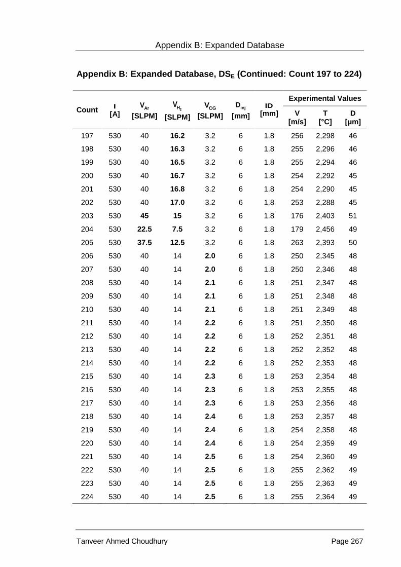
Appendix B: Expanded Database
Tanveer Ahmed Choudhury Page 267
Appendix B: Expanded Database, DSE (Continued: Count 197 to 224)
Count I [A]
ArV[SLPM]
2HV[SLPM]
CGV[SLPM]
injD [mm]
ID[mm]
Experimental Values
V [m/s]
T [°C]
D [μm]
197 530 40 16.2 3.2 6 1.8 256 2,298 46
198 530 40 16.3 3.2 6 1.8 255 2,296 46
199 530 40 16.5 3.2 6 1.8 255 2,294 46
200 530 40 16.7 3.2 6 1.8 254 2,292 45
201 530 40 16.8 3.2 6 1.8 254 2,290 45
202 530 40 17.0 3.2 6 1.8 253 2,288 45
203 530 45 15 3.2 6 1.8 176 2,403 51
204 530 22.5 7.5 3.2 6 1.8 179 2,456 49
205 530 37.5 12.5 3.2 6 1.8 263 2,393 50
206 530 40 14 2.0 6 1.8 250 2,345 48
207 530 40 14 2.0 6 1.8 250 2,346 48
208 530 40 14 2.1 6 1.8 251 2,347 48
209 530 40 14 2.1 6 1.8 251 2,348 48
210 530 40 14 2.1 6 1.8 251 2,349 48
211 530 40 14 2.2 6 1.8 251 2,350 48
212 530 40 14 2.2 6 1.8 252 2,351 48
213 530 40 14 2.2 6 1.8 252 2,352 48
214 530 40 14 2.2 6 1.8 252 2,353 48
215 530 40 14 2.3 6 1.8 253 2,354 48
216 530 40 14 2.3 6 1.8 253 2,355 48
217 530 40 14 2.3 6 1.8 253 2,356 48
218 530 40 14 2.4 6 1.8 253 2,357 48
219 530 40 14 2.4 6 1.8 254 2,358 48
220 530 40 14 2.4 6 1.8 254 2,359 49
221 530 40 14 2.5 6 1.8 254 2,360 49
222 530 40 14 2.5 6 1.8 255 2,362 49
223 530 40 14 2.5 6 1.8 255 2,363 49
224 530 40 14 2.5 6 1.8 255 2,364 49

Appendix B: Expanded Database
Tanveer Ahmed Choudhury Page 268
Appendix B: Expanded Database, DSE (Continued: Count 225 to 252)
Count I [A]
ArV[SLPM]
2HV[SLPM]
CGV[SLPM]
injD [mm]
ID[mm]
Experimental Values
V [m/s]
T [°C]
D [μm]
225 530 40 14 2.6 6 1.8 256 2,365 49
226 530 40 14 2.6 6 1.8 256 2,366 49
227 530 40 14 2.6 6 1.8 256 2,367 49
228 530 40 14 2.7 6 1.8 257 2,369 49
229 530 40 14 2.7 6 1.8 257 2,370 49
230 530 40 14 2.7 6 1.8 257 2,371 49
231 530 40 14 2.8 6 1.8 258 2,372 49
232 530 40 14 2.8 6 1.8 258 2,373 49
233 530 40 14 2.8 6 1.8 258 2,375 50
234 530 40 14 2.8 6 1.8 259 2,376 50
235 530 40 14 2.9 6 1.8 259 2,377 50
236 530 40 14 2.9 6 1.8 260 2,378 50
237 530 40 14 2.9 6 1.8 260 2,380 50
238 530 40 14 3.0 6 1.8 260 2,381 50
239 530 40 14 3.0 6 1.8 261 2,382 50
240 530 40 14 3.0 6 1.8 261 2,384 50
241 530 40 14 3.1 6 1.8 261 2,385 50
242 530 40 14 3.1 6 1.8 262 2,386 50
243 530 40 14 3.1 6 1.8 262 2,388 50
244 530 40 14 3.1 6 1.8 262 2,389 51
245 530 40 14 3.2 6 1.8 263 2,390 51
246 530 40 14 3.2 6 1.8 263 2,391 51
247 530 40 14 3.2 6 1.8 264 2,393 51
248 530 40 14 3.3 6 1.8 264 2,394 51
249 530 40 14 3.3 6 1.8 264 2,395 51
250 530 40 14 3.3 6 1.8 265 2,397 51
251 530 40 14 3.4 6 1.8 265 2,398 51
252 530 40 14 3.4 6 1.8 265 2,399 51

Appendix B: Expanded Database
Tanveer Ahmed Choudhury Page 269
Appendix B: Expanded Database, DSE (Continued: Count 253 to 280)
Count I [A]
ArV[SLPM]
2HV[SLPM]
CGV[SLPM]
injD [mm]
ID[mm]
Experimental Values
V [m/s]
T [°C]
D [μm]
253 530 40 14 3.4 6 1.8 266 2,401 51
254 530 40 14 3.4 6 1.8 266 2,402 51
255 530 40 14 3.5 6 1.8 267 2,403 51
256 530 40 14 3.5 6 1.8 267 2,405 52
257 530 40 14 3.5 6 1.8 267 2,406 52
258 530 40 14 3.6 6 1.8 268 2,407 52
259 530 40 14 3.6 6 1.8 268 2,408 52
260 530 40 14 3.6 6 1.8 268 2,410 52
261 530 40 14 3.7 6 1.8 269 2,411 52
262 530 40 14 3.7 6 1.8 269 2,412 52
263 530 40 14 3.7 6 1.8 270 2,414 52
264 530 40 14 3.7 6 1.8 270 2,415 52
265 530 40 14 3.8 6 1.8 270 2,416 52
266 530 40 14 3.8 6 1.8 271 2,417 52
267 530 40 14 3.8 6 1.8 271 2,419 53
268 530 40 14 3.9 6 1.8 271 2,420 53
269 530 40 14 3.9 6 1.8 272 2,421 53
270 530 40 14 3.9 6 1.8 272 2,422 53
271 530 40 14 4.0 6 1.8 272 2,423 53
272 530 40 14 4.0 6 1.8 273 2,425 53
273 530 40 14 4.0 6 1.8 273 2,426 53
274 530 40 14 4.0 6 1.8 273 2,427 53
275 530 40 14 4.1 6 1.8 274 2,428 53
276 530 40 14 4.1 6 1.8 274 2,429 53
277 530 40 14 4.1 6 1.8 274 2,430 53
278 530 40 14 4.2 6 1.8 275 2,432 53
279 530 40 14 4.2 6 1.8 275 2,433 53
280 530 40 14 4.2 6 1.8 275 2,434 54

Appendix B: Expanded Database
Tanveer Ahmed Choudhury Page 270
Appendix B: Expanded Database, DSE (Continued: Count 281 to 308)
Count I [A]
ArV[SLPM]
2HV[SLPM]
CGV[SLPM]
injD [mm]
ID[mm]
Experimental Values
V [m/s]
T [°C]
D [μm]
281 530 40 14 4.3 6 1.8 276 2,435 54
282 530 40 14 4.3 6 1.8 276 2,436 54
283 530 40 14 4.3 6 1.8 276 2,437 54
284 530 40 14 4.3 6 1.8 276 2,438 54
285 530 40 14 4.4 6 1.8 277 2,439 54
286 530 40 14 4.4 6 1.8 277 2,440 54
287 530 40 14 4.4 6 1.8 277 2,441 54
288 530 40 14 4.5 6 1.8 278 2,442 54
289 530 40 14 4.5 6 1.8 278 2,443 54
290 530 40 14 4.5 6 1.8 278 2,444 54
291 530 40 14 4.6 6 1.8 278 2,445 54
292 530 40 14 4.6 6 1.8 279 2,446 54
293 530 40 14 4.6 6 1.8 279 2,447 54
294 530 40 14 4.6 6 1.8 279 2,448 55
295 530 40 14 4.7 6 1.8 279 2,448 55
296 530 40 14 4.7 6 1.8 280 2,449 55
297 530 40 14 4.7 6 1.8 280 2,450 55
298 530 40 14 4.8 6 1.8 280 2,451 55
299 530 40 14 4.8 6 1.8 280 2,452 55
300 530 40 14 4.8 6 1.8 281 2,453 55
301 530 40 14 4.9 6 1.8 281 2,453 55
302 530 40 14 4.9 6 1.8 281 2,454 55
303 530 40 14 4.9 6 1.8 281 2,455 55
304 530 40 14 4.9 6 1.8 281 2,456 55
305 530 40 14 5.0 6 1.8 282 2,456 55
306 530 40 14 5.0 6 1.8 282 2,457 55
307 530 40 14 3.2 7 1.8 270 2,434 47
308 530 40 14 3.2 8 1.8 278 2,451 52
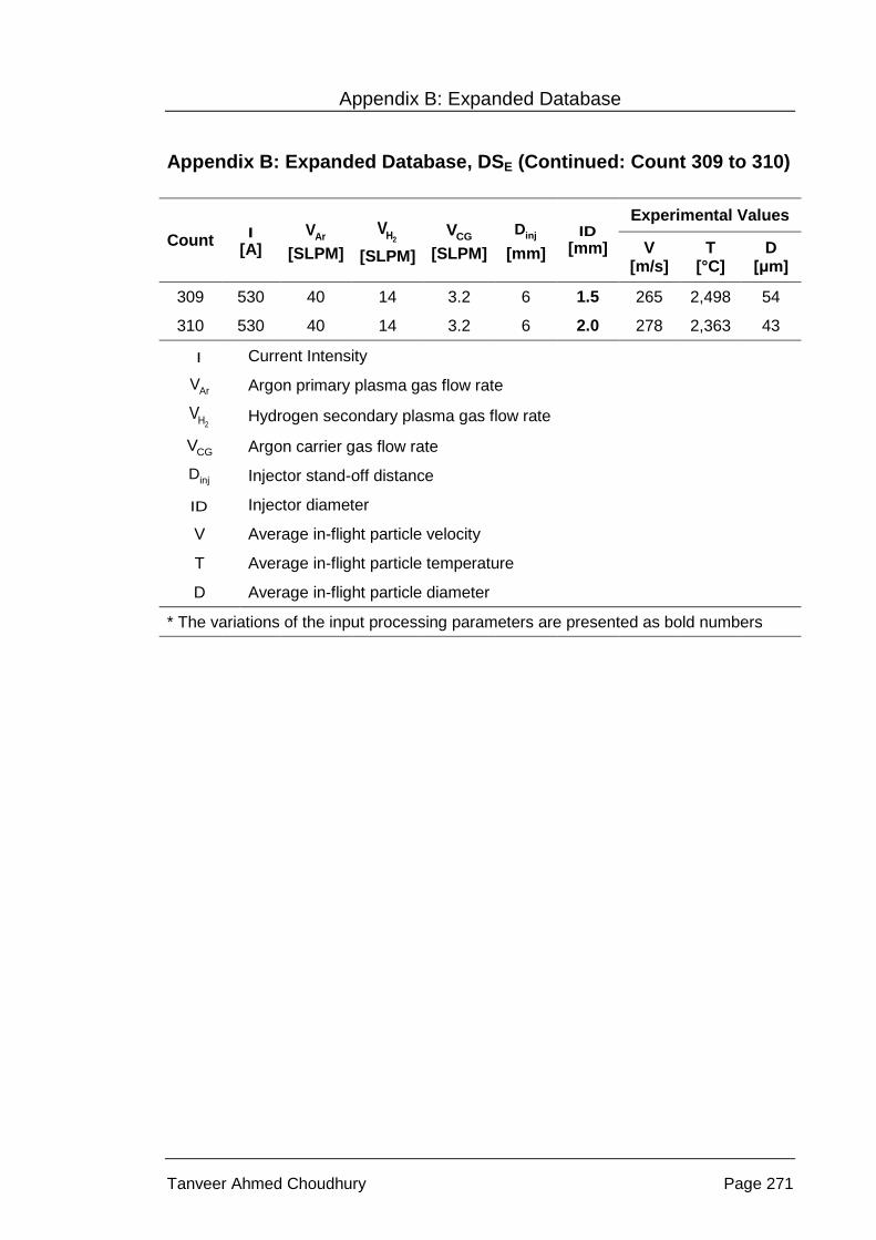
Appendix B: Expanded Database
Tanveer Ahmed Choudhury Page 271
Appendix B: Expanded Database, DSE (Continued: Count 309 to 310)
Count I [A]
ArV[SLPM]
2HV[SLPM]
CGV[SLPM]
injD [mm]
ID[mm]
Experimental Values
V [m/s]
T [°C]
D [μm]
309 530 40 14 3.2 6 1.5 265 2,498 54
310 530 40 14 3.2 6 2.0 278 2,363 43
I Current Intensity
ArV Argon primary plasma gas flow rate
2HV Hydrogen secondary plasma gas flow rate
CGV Argon carrier gas flow rate
injD Injector stand-off distance
ID Injector diameter
V Average in-flight particle velocity
T Average in-flight particle temperature
D Average in-flight particle diameter
* The variations of the input processing parameters are presented as bold numbers