Journal of Environmental Sciences 19(2007) 427–431

Artificial neural network model for identifying taxi gross emitter from remotesensing data of vehicle emission

ZENG Jun1, GUO Hua-fang1,2, HU Yue-ming1,∗

1. College of Automation Science and Engineering, South China University of Technology, Guangzhou 510640, China.E-mail: auzengjun@yahoo.com.cn

2. Automation Engineering Research and Manufacture Center, Guangdong Academy of Sciences, Guangzhou 510070, China

Received 10 April 2006; revised 12 June 2006; accepted 10 July 2006

AbstractVehicle emission has been the major source of air pollution in urban areas in the past two decades. This article proposes an

artificial neural network model for identifying the taxi gross emitters based on the remote sensing data. After carrying out the field

test in Guangzhou and analyzing various factors from the emission data, the artificial neural network modeling was proved to be an

advisable method of identifying the gross emitters. On the basis of the principal component analysis and the selection of algorithm

and architecture, the Back-Propagation neural network model with 8-17-1 architecture was established as the optimal approach for this

purpose. It gave a percentage of hits of 93%. Our previous research result and the result from aggression analysis were compared, and

they provided respectively the percentage of hits of 81.63% and 75%. This comparison demonstrates the potentiality and validity of the

proposed method in the identification of taxi gross emitters.

Key words: vehicle emission; remote sensing; neural network; principal component analysis; regression analysis

Introduction

Poor air quality has become a serious problem in

the world. Reports show that the on-road vehicle emis-

sions constitute the major source of air pollution in

urban areas. It contributes over 60% of the carbon

monoxides (CO), 30% of the hydrocarbons (HC), and

20% of the nitrogen oxides (NOx) in the national

records (USEPA, 1998; Pokharel et al., 2001a; Fish-

er, 2003). A recent investigation conducted by China

Environmental Protection Agency (CEPA) shows that

vehicle emissions account for 79% of air pollutants,

and this figure will remain air unchanged in the fu-

ture (CEPA, http://www.people.com.cn/GB/qiche/1049/

3021570.html). Further research shows that the majority

of the vehicle emissions come from the 10%–30% of the

used cars (Bishop et al., 1997; Calvert et al., 1993). They

are really the gross emitters.

In the last two decades, the national and local gov-

ernment have established various programs of inspection

and maintenance (I/M), as well as the total planning and

control standards. However, these programs have been

heavily criticized as costly or even wasteful, causing incon-

venience to the testers and drivers (Bishop and Stedman,

1996). Because the test data do not reflect the real emission

of running cars, many vehicles, which had passed the emis-

Project supported by the Key Technologies Research and Development

Program of Guangdong Province Foundation (No. 2003A3040301).

*Corresponding author. E-mail: auymhu@scut.edu.cn.

sion test in the test station, are playing the roles of gross

polluters in real world driving conditions (Washbum et al.,2001). Thus, researchers are looking for new methods for

collecting and analyzing the real-time emission data from

running cars.

One of these methods makes use of remote sensing

technique, which employed non-dispersed infrared instru-

ment in 1980s (Bishop et al., 1989) and tunable diode

laser system in 1998 (Nelson et al., 1998) to acquire the

real-time data of vehicle emission in driving conditions.

This technique has been widely applied in the United

States, Canada, Mexico, Australia and so on (Chan etal., 2002). On the other hand, new methods for analyzing

vehicle emission data were developed. The emission-factor

models based on dynamometer test, MOBILE (USEPA,

1993) and EMFAC (CARB, 1996), have been widely

employed to evaluate air quality in North America (Yu,

1998). The relation between emission intensity and driving

speed was investigated by Andre (2000) in Europe. Yu

(1998) developed an on-road model for estimating the

CO, HC emission rate from the vehicle speed. Researchers

in Tsinghua University have explored the characteristic

and effects of vehicle emissions in Beijing and Macao

(Hao et al., 2001). For the remote sensing data, people in

Denver University have done a series of experiments and

analysis of the remote sensing data collected from different

district in Denver (Pokharel et al., 2002, 2001b), Chicago

(Pokharel et al., 2000) and Los Angeles (Pokharel et al.,2001a).

428 ZENG Jun et al. Vol. 19

The remote-sensing system of vehicle emissions were

also applied in several major cities in China. This paper

analyzes the factors affecting vehicle emissions based on

the remote sensing test data of taxi emissions from a field

test in Guangzhou, Guangdong Province, China during the

year of 2004. It also proposes a model for identifying the

on-road gross emitters by combing the remote-sensing data

and the idle test data, once a set of vehicle remote sensing

characteristics were given. The percentage of hits reaches

93%. The model can be used as a ground-work for the

identification of gross emitters in I/M system.

1 Field data acquisition

1.1 On-site measurement

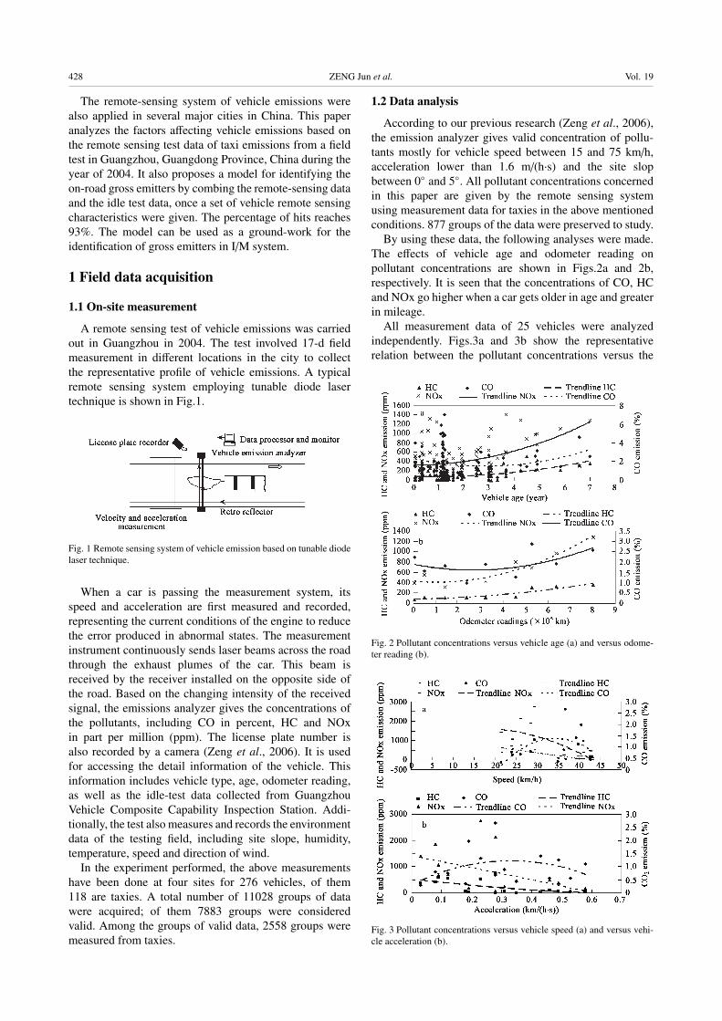
A remote sensing test of vehicle emissions was carried

out in Guangzhou in 2004. The test involved 17-d field

measurement in different locations in the city to collect

the representative profile of vehicle emissions. A typical

remote sensing system employing tunable diode laser

technique is shown in Fig.1.

Fig. 1 Remote sensing system of vehicle emission based on tunable diode

laser technique.

When a car is passing the measurement system, its

speed and acceleration are first measured and recorded,

representing the current conditions of the engine to reduce

the error produced in abnormal states. The measurement

instrument continuously sends laser beams across the road

through the exhaust plumes of the car. This beam is

received by the receiver installed on the opposite side of

the road. Based on the changing intensity of the received

signal, the emissions analyzer gives the concentrations of

the pollutants, including CO in percent, HC and NOx

in part per million (ppm). The license plate number is

also recorded by a camera (Zeng et al., 2006). It is used

for accessing the detail information of the vehicle. This

information includes vehicle type, age, odometer reading,

as well as the idle-test data collected from Guangzhou

Vehicle Composite Capability Inspection Station. Addi-

tionally, the test also measures and records the environment

data of the testing field, including site slope, humidity,

temperature, speed and direction of wind.

In the experiment performed, the above measurements

have been done at four sites for 276 vehicles, of them

118 are taxies. A total number of 11028 groups of data

were acquired; of them 7883 groups were considered

valid. Among the groups of valid data, 2558 groups were

measured from taxies.

1.2 Data analysis

According to our previous research (Zeng et al., 2006),

the emission analyzer gives valid concentration of pollu-

tants mostly for vehicle speed between 15 and 75 km/h,

acceleration lower than 1.6 m/(h·s) and the site slop

between 0◦ and 5◦. All pollutant concentrations concerned

in this paper are given by the remote sensing system

using measurement data for taxies in the above mentioned

conditions. 877 groups of the data were preserved to study.

By using these data, the following analyses were made.

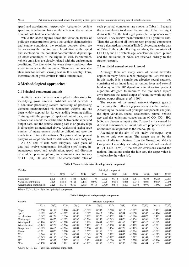
The effects of vehicle age and odometer reading on

pollutant concentrations are shown in Figs.2a and 2b,

respectively. It is seen that the concentrations of CO, HC

and NOx go higher when a car gets older in age and greater

in mileage.

All measurement data of 25 vehicles were analyzed

independently. Figs.3a and 3b show the representative

relation between the pollutant concentrations versus the

Fig. 2 Pollutant concentrations versus vehicle age (a) and versus odome-

ter reading (b).

Fig. 3 Pollutant concentrations versus vehicle speed (a) and versus vehi-

cle acceleration (b).

No. 4 Artificial neural network model for identifying taxi gross emitter from remote sensing data of vehicle emission 429

speed and acceleration, respectively. Apparently, vehicle

speed and acceleration have similar effects on the variation

trend of pollutant concentrations.

While the above figures show the variation trends of

pollutant concentrations versus the vehicle characteristics

and engine conditions, the relations between them are

by no means the precise ones. In addition to the speed

and acceleration, the pollutant concentrations depend up-

on other conditions of the engine as well. Furthermore,

vehicle emissions are closely related with the environment

conditions. The interaction between these conditions also

gives impacts on the emission. There are no available

standards for remote sensing test in this country. Thus,

identification of gross emitter is still a difficult task.

2 Methodological approaches

2.1 Principal component analysis

Artificial neural network was applied in this study for

identifying gross emitters. Artificial neural network is

a nonlinear processing system consisting of processing

elements interconnected via connection weights and has

been widely applied for its outstanding learning ability.

Training with the groups of input and output data, neural

network can encode the relationship between the input and

output data. But the remote sensing data is originally high

in dimension as mentioned above. Analysis of such a large

number of measurements would be difficult and take too

much time to train the network. So, principal component

analysis was applied at first for data reduction and analysis.

All 877 sets of data were analyzed. Each piece of

data had twelve components, including sites’ slope, in-

stantaneous speed and acceleration, speed and direction

of wind, temperature, plume, and emission concentrations

of CO, CO2, HC and NOx. The characteristic rates of

each principal component are shown in Table 1. Because

the accumulative total contribution rate of the first eight

items is 89.7%, the first eight principle components were

selected. They reserve the information of all primitive data.

Then, the weights of all items to each principal component

were calculated, as shown in Table 2. According to the data

of Table 2, the eight effecting variables, the emissions of

CO, CO2 and HC, vehicle age, acceleration, speed, plume

and the emissions of NOx, are reserved orderly to the

further research.

2.2 Artificial neural network model

Although there are many kinds of neural networks

applied in many fields, a back-propagation (BP) was used

in this study. It is a simple but effective neural network,

consisting of an input layer, an output layer and several

hidden layers. The BP algorithm is an interactive gradient

algorithm designed to minimize the root mean square

error between the actual output of neural network and the

desired output (Hagan et al., 1996).

The success of the neural network depends greatly

on defining the influencing parameters for the problem.

According to the results of principle components analysis,

the eight variables, speed, acceleration, plume, vehicle

age and the emissions concentration of CO, CO2, HC,

NOx, are chosen as input units. To avoid error caused by

different dimensions, all input data are preprocessed, and

normalized in amplitude to the interval [0, 1].

According to the aim of this study, the output layer

is set to only one union. The targets are set by the

results of idle test obtained from the Guangzhou Vehicle

Composite Capability according to the national standard

(GB/T 14761.5-93). If the vehicle emissions exceed the

national limitations under the idle test, the target value is

1, otherwise the value is 0.

Table 1 Characteristic rates of each primary component

Variable Principal component

X(1) X(2) X(3) X(4) X(5) X(6) X(7) X(8) X(9) X(10) X(11) X(12)

Latent root 2.695 1.843 1.458 1.383 1.194 0.905 0.714 0.576 0.511 0.395 0.323 0.003

Variance contribution 0.225 0.154 0.121 0.115 0.099 0.075 0.059 0.048 0.043 0.033 0.027 0.000

Accumulative contribution 0.225 0.378 0.500 0.615 0.714 0.790 0.849 0.897 0.940 0.973 1.000 1.000

Where, X(I=1, 2, 3···12) is the I principal component.

Table 2 Weights of each principle component

Variable Principal component

X(1) X(2) X(3) X(4) X(5) X(6) X(7) X(8) X(9) X(10) X(11) X(12)

Slope –0.350 0.158 0.160 –0.406 –0.082 0.282 0.380 0.313 –0.007 0.391 0.425 –0.001

Speed 0.022 –0.313 –0.567 0.148 0.027 0.412 0.174 0.284 –0.050 0.305 –0.426 –0.002

Acceleration 0.047 –0.179 0.056 0.335 0.702 0.326 –0.152 0.010 –0.066 –0.023 0.473 0.001

Vehicle age –0.039 0.475 –0.079 0.263 –0.284 0.183 –0.543 0.070 –0.454 0.268 0.075 0.000

Wind speed –0.186 0.328 –0.268 –0.350 0.103 0.451 –0.312 –0.165 0.467 –0.315 –0.089 0.000

Wind direction –0.145 0.228 –0.306 –0.209 0.422 –0.515 –0.130 0.549 –0.119 –0.103 –0.061 0.002

Temperature –0.063 0.415 –0.384 0.087 0.230 –0.139 0.454 –0.578 –0.183 0.146 0.041 0.005

Plume –0.291 0.076 0.520 –0.113 0.357 0.168 0.011 –0.099 –0.304 0.052 –0.605 -0.003

CO 0.544 0.150 0.038 –0.244 0.042 0.174 0.122 0.093 –0.210 –0.140 –0.013 0.708

CO2 –0.543 –0.155 –0.034 0.241 –0.044 –0.172 –0.127 –0.092 0.212 0.147 0.009 0.706

HC 0.337 0.352 0.217 0.218 0.171 –0.098 –0.006 0.123 0.578 0.502 –0.166 –0.003

NOx –0.158 0.334 0.105 0.530 –0.132 0.155 0.395 0.335 0.070 –0.504 -0.052 0.005

Where, X(I=1, 2, 3···12) is the I principal component.

430 ZENG Jun et al. Vol. 19

Then, 17 unions are chosen in the hidden layer accord-

ing to Kolmgorov’s theory. The Kolmogorov’s mapping

neural network existence theorem states that given any

continuous function f : [0, 1]n → Rm, f (x) = y, f can be

implemented exactly by a three layer, (2n+1) processing

elements in the middle layer, and m processing elements in

the output layer (Nielsen, 1987).

Furthermore, it has been proved that a three layer neural

network, having sigmoid units in its hidden layer has been

shown mathematical to approximate any given real valued

continuous multi-variable function to the projected degree

of accuracy (Hagan et al., 1996). And compared with the

performance of different network algorithms, the improved

BP neural network with Levenberg-Marquardt algorithm

was chosen.

Finally, 300 groups of data are chosen. Of them 200 are

used as training data and the remained 100 are used as the

test data.

The Matlab 7 attached with the neural network toolbox

(edition 4.0.3) is used in the work to establish the model.

The experimental results show that the performance goal

is obtained at the 37th epoch. Test results show that the

percentage of hits is up to 93%. Fig.4 shows the training

error curve. And Fig.5 represents the error distribution of

the test.

Fig. 4 Training error curve.

Fig. 5 Error distribution of the test.

3 Comparison and discussion

This BP neural network model based on taxies data

is capable of identifying gross emitters using remote-

sensing data. The percentage of hits of 93% is better

than the 81.63% obtained from our former research (Guo

et al., 2006) based on the same experimental data. The

difference between the two results shows that the data

pre-processing and correct classification of vehicles are

very important. Different characteristics in usage, different

categories models of gross emitters should be established

respectively. Then, high accuracy would be achieved.

Regression analysis was believed as another useful

method to identify the characteristics of vehicles that are

more likely to be gross emitters. During this research,

regression analysis acquires the percentage of hits of 75%

using the same groups of data. The amendment simultane-

ous equation is as follows.

Y = −0.0266x1 − 0.0155x2 + 0.1834x3 + 0.1289x4 + 0.5644x5+

0.1502x6 + 0.3421x7 + 0.2173x8 − 0.13538

Where, the sequence of xi (i=1, 2, 3···8) denotes speed,

acceleration, plume, vehicle age, the emission of CO, CO2,

HC, NOx, respectively. Y is the output.

The results show that neural network model performs

better than the regression analysis model. In sum, the BP

neural network is capable of predicting vehicle emission

based on remote-sensing data. The results also imply

that remote-sensing data is suitable for emission model

evaluation.

4 Conclusions

In this paper, we adopt artificial neural network to identi-

fy the gross emitters with vehicle emission remote-sensing

data from Guangzhou, Guangdong Province. Vehicle emis-

sion is a complex multivariable nonlinear process. The

BP neural network model is a valid model with good

prediction ability. The experimental results show that the

performance goal is obtained at the 37th epoch, and the

percentage of hits is up to 93%. The findings also indicate

that speed, acceleration, plume and vehicle age play a

significant role in determining the prediction results, as

well as the emissions concentration of CO, CO2, HC and

NOx.

Vehicle emission is the major source of air pollution

today and in the future. Pollution control is very impor-

tant in improving air quality. This model identifies gross

emitter effectively. Our work can be used as groundwork

for identifying gross taxies’ emitters. Then it can reduce

the cost and improve efficiency of in-use I/M system.

Other catalogues vehicle gross emitter identification model

should be established in our future research. More reli-

able remote-sensing data will be accumulated with more

advanced test technique, intelligent algorithm and data

mining technology.

Acknowledgements: The authors are extended to thank

Prof. Tu Qili for his instruction and efforts in editing the

English of this manuscript.

No. 4 Artificial neural network model for identifying taxi gross emitter from remote sensing data of vehicle emission 431

References

Andre M, 2000. Driving speeds in Europe for pollutant emissions

estimation[J]. Transportation Research, Part D: Transport

and Environment, 5(5): 321–335.

Bishop G A, Aldermen P, Slot R, 1997. On-road evaluation of

an automobile emission test program[J]. Enviro Sci and

Technol, (31): 927–931.

Bishop G A, Stedman D H, 1996. Measuring the emissions of

passing cars[J]. Acc Chem Res, 29: 489–495.

Bishop G A, Starkey J R, Williams W J et al., 1989, IR long

path photometry: a remote sensing tool for automobile

emissions[J]. Anal Chem, 61: 671A–677A.

Calvert J, Heywood J, Sewer R et al., 1993. Achieving acceptable

air quality: some reflections on controlling vehicle emis-

sions[J]. Science, 261: 37–45.

CARB (California Air Resource Board), 1996. Methodology for

estimating emissions from on-road motor vehicles[Z]. Pre-

pared by technical support division, mobile source emission

inventory branch, Calfornia air resources board.

CEPA (China Environment Protection Agency)[EB]. http://

www.people.com.cn/GB/qiche/1049/3021570.html.

Chan T L, Dong G, Ning Z et al., 2002. On-road remote sensing

of petrol vehicle emission measurement and emission fac-

tors estimation for urban driving patterns in Hong Kong[R].

Better Air Quality in Asian and Pacific Rim Cities (BAQ

2002), Hong Kong SAR.

Fisher G W, Bluest J G, Xiao S et al., 2003. On-road remote

sensing of vehicle emissions in the Auckland region[R].

Auckland Regional Council Technical Publication, No.198.

Guo H F, Zeng J, Hu Y M, 2006. Neural network modeling of

vehicle gross emitter prediction based on remote sensing

data[C]. IEEE International Conference on Networking,

Sensing and Control, Florida, USA. 943–946.

Hagan M T, Demuth H B, Beale M, 1996. Neural network

design[M]. Beijing: China Machine Press and CITOC Pub-

lishing House.

Hao J M, Fu L X, He K B et al., 2001. Vehicle pollutants emission

control[M]. Beijing: China Environment Science Publishing

Company.

Nelson D D, Zahniser M S, Mcmanus J B et al., 1998. A tunable

diode laser system for the remote sensing of on-road vehicle

emissions[J]. Appl Phys, B67: 433–441.

Nielsen R H, 1987. Kolmogorovns’ mapping neural network

existing theorem[C]. In Proc. of the Int. Conf. on Neural

Networks, III, IEEE Press, New York, 11–13.

Pokharel S S, Bishop G A, Stedman D H, 2000. On-road remote

sensing of automobile emissions in the Chicago area: Year

3[R]. Coordinating Research Council, No. E-23-4. 1–25.

Pokharel S S, Bishop G A, Stedman D H, 2001a. On-road remote

sensing of automobile emission in the los angeles area:

year 2[R]. Coordinating Research Council, No. E-23-4.

Alpharetta, GA Inc, March 2001.

Pokharel S S, Bishop G A, Stedman D H, 2001b. Fuel-based

on-road motor vehicle emissions inventory for the Denver

Metropolitan area[Z]. Contract No. E-11-4. 1–15.

Pokharel S S, Bishop G A, Stedman D H, 2002. An on-road

motor vehicle emissions inventory for Denver: an efficient

alternative to modeling[J]. Atmospheric Environment, 30:

5177–5184.

USEPA (United States Environmental Protection Agency), 1993.

User’s guide to Mobile5A[Z]. Mobile source emission

factor model.

USEPA (United States Environmental Protection Agency), 1998,

National air quality and emissions trends[S]. Research

Triangle Park, NC, 2000; EPA-455/R-00-003, 11–37.

Washburn S, Seet J, Mannering F, 2001. Statistical modeling

of vehicle emissions from inspection/maintenance testing

data: An exploratory analysis[J]. Transportation Research,

Part D: Transport and Environment, 6(1): 21–36.

Yu L, 1998. Remote vehicle exhaust emission sensing for traffic

simulation and optimization models[J]. Transportation Re-

search, Part D: Transport and Environment, 3(5): 337–347.

Zeng J, Guo H F, Hu Y M, 2006. A remote sensing system of ve-

hicle emissions based on tunable diode laser technology[J].

Journal of Environmental Sciences, 18(1): 154–157.