artificial boundary method || applications to problems with singularity

Chapter 9

Applications to Problemswith Singularity

Abstract: In this chapter, we discuss the application of ABCs for some prob-lems with singularity, including the modified Helmholtz equation with singu-larity, the interface problem, the linear elastic system with singularity, andthe Stokes equations with singularity. By using artificial boundaries, the sin-gular points are removed, and the original problems are reduced to boundaryvalue problems on computational domains. Boundary conditions on the artificialboundaries are obtained, and then the finite element method is applied to solvethe reduced problems. Some error estimates are also given.

Key words: Modified Helmholtz equation, interface problem, linear elasticsystem, Stokes equations, singularity.

The need to solve partial differential equations with singular solutions iscreated in many applications. For example, in the linear theory of fracture me-chanics (Anderson, 1995), we need to study the stress of the elastic body withcracks. At the endpoint of the crack we see the concentration of the stress.Moreover, the stress is unbounded at this point. This indicates that the solutionto the linear elastic system is singular. The singularity in these kinds of prob-lems makes the numerical solution difficult. The artificial boundary method isone of the efficient ways to solve this problem. In this chapter, we discuss theapplication of the artificial boundary method to problems with singularities.

Artificial Boundary Method© Tsinghua University Press, Beijing and Springer-Verlag Berlin Heidelberg 2013

H. Han et al.,

Artificial Boundary Method

9.1 The Modified Helmholtz Equation with aSingularity

In this section, we discuss the numerical solution of the modified Helmholtz equa-tion on bounded domains. When the solution domain has a corner, then, thesolution of this problem may be singular. In another case, when the boundarycondition is switched from one type to another type, for example, the Dirichletboundary condition is switched to the Neumann boundary condition at somepoint, then the solution may also be singular at this point. Assume that Ω ⊂ R2

is a bounded domain (as shown in Fig. 9-1), Γ = ΓD ∪ ΓN is the boundaryof Ω . Assume that the Dirichlet boundary condition and the Neumann bound-ary condition are given on ΓD and ΓN , respectively, we consider the followingproblem:

−Δu + a20u = f in Ω , (9.1.1)

u = 0 on ΓD, (9.1.2)

∂u

∂n= h on ΓN , (9.1.3)

where f ∈ L2(Ω), h ∈ L2(ΓN), and a0 is a nonnegative real number. Let

V ={v ∈ H1(Ω) | v = 0 on ΓD

}.

Then, the variational form of problem (9.1.1)∼(9.1.3) is⎧⎪⎨⎪⎩Find u ∈ V, such that∫Ω

(∇u∇v + a20uv) dx =

∫Ω

fv dx +∫ΓN

hv ds, ∀v ∈ V.(9.1.4)

In general, the solution u of the variational problem (9.1.4) is in H1(Ω), but notin Hk(Ω) for k � 2. Thus, the standard finite element method can not producesatisfactory numerical results for the variational problem (9.1.4), especially nearthe singular point. In the following, we discuss how to get accurate numericalresults by using artificail boundary method.

Fig. 9-1 Domain Ω

366

Chapter 9 Applications to Problems with Singularity

9.1.1 ABC Near Singular Points

In Ω , we introduce the artificial boundary ΓR = {x| x ∈ Ω , |x| = R}, whichdivides Ω into two parts (see Fig. 9-2(a)):

Ωi = {x | x ∈ Ω , |x| < R} ,

Ωe = {x | x ∈ Ω , |x| > R} .

(a) Domain Ωi and Ωe (b) Artificial boundary Γ1 and domain Ω1e

Fig. 9-2

Suppose that f = 0 in Ωi. Under the polar coordinates the restriction on Ωi

of the solution of problem (9.1.1)∼(9.1.3) satisfies

−Δu + a20u = 0 in Ωi, (9.1.5)

u = 0 on Γ0, (9.1.6)u = u(R, θ) ≡ uR(θ), on ΓR. (9.1.7)

The solution of problem (9.1.5)∼(9.1.7) can be expanded as follows:

u(r, θ) =∞∑

n=1

bngn(r) sin(

nθ

ω

), (9.1.8)

where ωπ is the interior angle of the singular point,

gn(r) = rn/ω , a0 = 0

gn(r) = In/ω(a0r) =(a0r

2

)n/ω ∞∑i=0

(a0r)2i

4ii!Γ (i + 1 + n/ω), a0 > 0.

If a0 > 0, In/ω(a0r) is the modified first kind Bessel function of order n/ω. From(9.1.7) we get the expression for bn, n = 1, 2, · · · :

bn =2

πωgn(R)

∫ ωπ

0

uR(φ) sin(

nφ

ω

)dφ,

367


where R is the radius of the circular arc ΓR. Thus, we get the solution of(9.1.5)∼(9.1.7):

u(r, θ) =∞∑

n=1

2gn(r)πωgn(R)

sin(

nθ

ω

)∫ ωπ

0

uR(φ) sin(

nφ

ω

)dφ

:=H(uR, r, θ). (9.1.9)

Restricted on ΓR, it is

u(R, θ) = H(uR, R, θ). (9.1.10)

The equality (9.1.10) is the condition on ΓR satisfied by the solution of problem(9.1.1)∼(9.1.3).

9.1.2 An Iteration Method Based on the ABC

Using (9.1.9) we can construct an iteration method for solving problem (9.1.1)∼(9.1.3).For simplicity, we assume that problem (9.1.1)∼(9.1.3) has only one singularpoint at the origin (Fig. 9-1) and ΓN = ∅. Introduce artificial boundary Γ1, asshown in Fig. 9-2(b). Γ1 is a circular art with radius R1, such that 0 < R1 < R.Let

Ω1e = {x | x ∈ Ω , |x| > R1} .

Suppose that the support of f is in Ωe, and u = 0 on Γ0. From (9.1.9) we canget the restriction on Γ1 of the solution u of problem (9.1.1)∼(9.1.3):

u(R1, θ) = H(uR, R1, θ).

Then, restricted on Ωe, problem (9.1.1)∼(9.1.3) is equivalent to the followingproblem:

−Δu + a20u = f in Ω1

e , (9.1.11)

u = 0 on Γ0 ∪ Γ , (9.1.12)

u = H(uR, R1, θ) on Γ1. (9.1.13)

Since uR is unknown, we construct the following iteration to solve problem(9.1.1)∼(9.1.3):

−Δu(k) + a20u

(k) = f in Ω1e , (9.1.14)

u(k) = 0 on Γ0 ∪ Γ , (9.1.15)

u(k) = H(u(k−1)R , R1, θ) on Γ1, (9.1.16)

368


where u(k−1)R = u(k−1)(R, θ). Let

V1 ={v ∈ H1(Ω1

e ) | v = 0 on Γ0 ∪ Γ ∪ Γ1

},

V(k)1 =

{v ∈ H1(Ω1

e ) | v = 0 on Γ0 ∪ Γ , v = H(u(k−1)R , R1, θ) on Γ1

}.

Then, the variational form of (9.1.14)∼(9.1.16) is{Given u

(k−1)R , find u(k) ∈ V

(k)1 , such that

a1(u(k), v) = (f, v), ∀v ∈ V1,(9.1.17)

wherea1(u, v) =

∫Ωe

(∇u∇v + a20uv)dx, (f, v) =

∫Ωe

fv dx.

It is not difficult to see that the above iteration is equivalent to the followingSchwarz alternating iteration method:

−Δu(k)1 + a2

0u(k)1 = f in Ωe, (9.1.18)

u(k)1 = 0 on Γ0 ∪ Γ , (9.1.19)

u(k)1 = u

(k−1)2 on Γ1, k = 1, 2, · · · , (9.1.20)

and

−Δu(k)2 + a2

0u(k)2 = f in Ωi, (9.1.21)

u(k)2 = 0 on Γ0, (9.1.22)

u(k)2 = u

(k)1 on ΓR, k = 1, 2, · · · . (9.1.23)

For the solution u(k)1 ∈ H1(Ωe) of (9.1.18)∼(9.1.20), let

u(k)1 (x) =

{u

(k)1 (x), x ∈ Ωe,

u(k−1)2 (x), x ∈ Ω \ Ωe.

Then, we extend u(k)1 to the domain Ω , and u

(k)1 ∈ V . For the solution u

(k)2 ∈

H1(Ωi) of (9.1.21)∼(9.1.23), let

u(k)2 (x) =

{u

(k)2 (x), x ∈ Ωi,

u(k)1 (x), x ∈ Ω \ Ωi.

Then, we extend u(k)2 to the domain Ω , and u

(k)2 ∈ V . Let

V2 ={v ∈ H1(Ωi) | v = 0 on ΓR ∪ Γ0

}.

369


Then,u

(k)1 − u

(k−1)2 ∈ V1, u

(k)2 − u

(k)1 ∈ V2.

Introducing the bilinear form

a2(u, v) =∫Ωi

(∇u∇v + a20uv)dx,

then, problem (9.1.18)∼(9.1.20) and problem (9.1.21)∼(9.1.23) are equivalent tothe following variational problems:{

Find u(k)1 such that u

(k)1 − u

(k−1)2 ∈ V1 and

a1(u(k)1 − u, v1) = 0, ∀v1 ∈ V1,

(9.1.24)

and {Find u

(k)2 such that u

(k)2 − u

(k)1 ∈ V2 and

a2(u(k)2 − u, v2) = 0, ∀v2 ∈ V2,

(9.1.25)

where u is the solution of problem (9.1.1)∼(9.1.3). Let PVi : V → Vi, i = 1, 2,denote the projection operator form the inner product space V to the innerproduct space Vi. Then, from (9.1.24) and (9.1.25), we obtain{

Find u(k)1 such that u

(k)1 − u

(k−1)2 ∈ V1 and

a1(u(k)1 − u

(k−1)2 , v1) = a1(u − u

(k−1)2 , v1), ∀v1 ∈ V1,

and {Find u

(k)2 such that u

(k)2 − u

(k)1 ∈ V2 and

a2(u(k)2 − u

(k)1 , v2) = a2(u − u

(k)1 , v2), ∀v2 ∈ V2.

Obviously, we have

u(k)1 − u

(k−1)2 = PV1(u − u

(k−1)2 ), (9.1.26)

u(k)2 − u

(k)1 = PV2(u − u

(k)1 ), k = 1, 2, · · · . (9.1.27)

Since u − u(k−1)2 = u − u

(k)1 + u

(k)1 − u

(k−1)2 and u

(k)1 − u

(k−1)2 ∈ V1, we have

u−u(k)1 ∈ V ⊥

1 . Similarly, u−u(k)2 ∈ V ⊥

2 , where V ⊥i is the orthogonal complement

of Vi in V . Therefore, equations (9.1.26) and (9.1.27) are equivalent to

u − u(k)1 = PV ⊥

1(u − u

(k−1)2 ), (9.1.28)

u − u(k)2 = PV ⊥

2(u − u

(k)1 ), k = 1, 2, · · · . (9.1.29)

Lete(k)i = u − u

(k)i , i = 1, 2.

370


Then, equations (9.1.28) and (9.1.29) become

e(k)1 = PV ⊥

1e(k−1)2 , (9.1.30)

e(k)2 = PV ⊥

2e(k)1 , k = 1, 2, · · · . (9.1.31)

Thus, we have

e(k+1)1 = PV ⊥

1PV ⊥

2e(k)1 , k = 1, 2, · · · , (9.1.32)

e(k+1)2 = PV ⊥

2PV ⊥

1e(k)2 , k = 0, 1, · · · . (9.1.33)

It is easy to see from equations (9.1.30) and (9.1.31) that if{e(k)i

}, i = 1, 2,

converges, then, the limit is in V ⊥1 ∩ V ⊥

2 . Similar to the proof of Lions (1988)and Yu (1994-A), we get

Theorem 9.1.1 limk→∞

∥∥∥e(k)i

∥∥∥1

= 0, i = 1, 2.

Theorem 9.1.2 There exists a constant α, 0 � α < 1, such that∥∥∥e(k)1

∥∥∥1

� αk−1∥∥∥e(1)

1

∥∥∥1,

∥∥∥e(k)2

∥∥∥1

� αk∥∥∥e(0)

2

∥∥∥1.

Theorem 9.1.1 and Theorem 9.1.2 show that the above Schwarz alternatingiteration method converges geometrically. In general, the constant α in the aboveestimate is not easy to determine. However, if Γ is a circular arc, then, we canobtain α. Suppose that Ωe is bounded by R1 � r � R2, 0 � θ � ωπ, where R2

is the radius of Γ . Assume that on Γ1 we have

e(0)2 (R1, θ) =

∞∑n=1

an sin(

nθ

ω

)

and e(1)1 (R2, θ) = 0 on Γ . Then, using separation of variables we get the expres-

sion for e(1)1 (r, θ) in Ωe:

e(1)1 (r, θ) =

∞∑n=1

(Anrn/ω + Bnr−n/ω

)sin(

nθ

ω

),

where

An =anR

n/ω1

R2n/ω1 − R

2n/ω2

, Bn =−anR

n/ω1 R

2n/ω2

R2n/ω1 − R

2n/ω2

.

Restricting on ΓR, we get

e(1)1 (R, θ) =

∞∑n=1

(AnRn/ω + BnR−n/ω

)sin(

nθ

ω

).

371


From equation (9.1.8), we have

e(1)2 (R1, θ) =

∞∑n=1

bnRn/ω1 sin

(nθ

ω

),

where

bn =2

ωπRn/ω

∫ ωπ

0

e(1)1 (R, φ) sin

(nφ

ω

)dφ

=1

Rn/ω

(AnRn/ω + BnR−n/ω

)=

anRn/ω1

(R2n/ω − R

2n/ω2

)R2n/ω

(R

2n/ω1 − R

2n/ω2

) .

Then, we have∥∥∥e(1)2

∥∥∥21/2,Γ1

=∞∑

n=1

(n2 + 1)1/2∣∣∣bnR

n/ω1

∣∣∣2=

∞∑n=1

(n2 + 1)1/2

∣∣∣∣∣an

(R1

R

)2n/ωR2n/ω − R

2n/ω2

R2n/ω1 − R

2n/ω2

∣∣∣∣∣2

�∞∑

n=1

(n2 + 1)1/2

∣∣∣∣∣an

(R1

R

)2n/ω∣∣∣∣∣2

�(

R1

R

)2/ω ∞∑n=1

(n2 + 1)1/2|an|2 =(

R1

R

)2/ω ∥∥∥e(0)2

∥∥∥21/2,Γ1

Similarly, we have ∥∥∥e(2)1

∥∥∥2

1/2,ΓR

�(

R

R2

)2/ω ∥∥∥e(1)1

∥∥∥21/2,ΓR

.

Thus, we obtain ∥∥∥e(k)2

∥∥∥1/2,Γ1

�(

R1

R

)k/ω ∥∥∥e(0)2

∥∥∥1/2,Γ1

,

∥∥∥e(k)1

∥∥∥1/2,ΓR

�(

R

R2

)(k−1)/ω ∥∥∥e(1)1

∥∥∥1/2,ΓR

.

Finally, using the trace theorem, we get∥∥∥e(k)2

∥∥∥1,Ωi

� C

(R1

R

)k/ω

,∥∥∥e(k)

1

∥∥∥1,Ωe

� C

(R

R2

)(k−1)/ω

.

The order of convergence of the iteration method depends on the ratios of theradius of the artificial boudaries ΓR, Γ1 and Γ2. Let R =

√R1R2 we get∥∥∥e(k)

2

∥∥∥1,Ωi

� C

(R1

R2

)k/2ω

,∥∥∥e(k)

1

∥∥∥1,Ωe

� C

(R1

R2

)(k−1)/2ω

.

372


9.2 The Interface Problem with a Singularity

If the coefficients of the partial differential equation are discontinuous, then, thesolution may be singular. A typical example of this is the interface problem.Assume that Ω is a bounded domain on the plane with Γ as its boundary(see Fig. 9-3). Under the polar coordinates we consider the following interfaceproblem:

−∇(p∇u) = f in Ω , (9.2.1)u = g on Γ , (9.2.2)u(r, φk − 0) = u(r, φk + 0), 1 � k � M, (9.2.3)

pk−1∂u

∂n(r, φk − 0) = pk

∂u

∂n(r, φk + 0), 1 � k � M, (9.2.4)

where the straight lines θ = φk, k = 1, 2, · · · , M are interfaces, which divide Ωinto subdomains Ω1, · · · ,ΩM , the coefficient p is a piecewise positive constantfunction, i.e., in Ωk, p = pk, k = 1, 2, · · · , M(p0 = pM ), and f and g are givenfunctions on Ω and Γ .

Introduce the following set and space:

H1g (Ω) = {v : v ∈ H1(Ω), v|Γ = g},

H10 (Ω) = {v : v ∈ H1(Ω), v|Γ = 0}.

Then, the boundary value problem (9.2.1)∼(9.2.4) is equivalent to the followingvariational problem:{

Find u ∈ H1g (Ω), such that

a(u, v) = (f, v) ∀v ∈ H10 (Ω), (9.2.5)

Fig. 9-3 Domain Ω and interfaces

where

a(u, v) =∫Ω

p∇u · ∇vdx, (f, v) =∫Ω

fvdx.

Since p is a positive function on Ω , the bilinear form a(u, v) is bounded andcoercive on H1

0 (Ω) × H10 (Ω), i.e., there exists a constant α > 0 such that

a(v, v) � α‖v‖21,Ω ∀v ∈ H1

0 (Ω)

373


Then, from Lax-Milgram theorem (Ciarlet, 1977) we get

Theorem 9.2.1 For given f ∈ H−1(Ω) and g ∈ H1/2(Γ ), the variational prob-lem (9.2.5) has a unique solution u ∈ H1

g (Ω).Since the coefficient p is discontinuous on Ω , the solution of the problem is

not in H2(Ω), and the intersection point of the interfaces is a singular point.In this section, we use the artificial boundary method to solve this problemnumerically.

9.2.1 A Discrete Boundary Condition on the ArtificialBoundary ΓR

We first introduce the artificial boundary ΓR = {x | |x| = R} (see Fig. 9-4),where R < R0 and Γ0 = {x | |x| = R0} ⊂ Ω . ΓR divides the domain Ω into twoparts: Ωi = {x | |x| < R} and Ωe = Ω \ Ωi.

Fig. 9-4 Artificial boundary ΓR

Assume that f = 0 in the domain Ωi. Then, the restriction on the domainΩi of the solution of problem (9.2.1)∼(9.2.4) satisfies

−∇(p∇u) = 0 in Ωi, (9.2.6)u = u(R, θ) on ΓR, (9.2.7)u(r, φk − 0) = u(r, φk + 0), 1 � k � M, (9.2.8)

pk−1∂u

∂n(r, φk − 0) = pk

∂u

∂n(r, φk + 0), 1 � k � M. (9.2.9)

For given u(R, θ) ∈ H1/2(ΓR), problem (9.2.6)∼(9.2.9) has a unique weak solu-

tion u, and∂u

∂n

∣∣∣∣ΓR

∈ H−1/2(ΓR). Thus, we get a bounded operator E:

E : H1/2(ΓR) → H−1/2(ΓR),

∂u

∂n

∣∣∣∣ΓR

= E(u|ΓR). (9.2.10)

374


Equation (9.2.10) is an exact boundary condition on ΓR satisfied by the solutionof problem (9.2.1)∼(9.2.4). However, it is difficult to find E in general. In therest of this subsection, we discuss how to find an approximation of E. Underthe polar coordinates, problem (9.2.6)∼(9.2.9) has the following form:

∂

∂r

(pr

∂u

∂r

)+

1r

∂

∂θ

(p∂u

∂θ

)= 0, (9.2.11)

u|r=R = u(R, θ), u is bounded, as r → 0, (9.2.12)u|θ=φk−0 = u|θ=φk+0, 1 � k � M, (9.2.13)

pk−1∂u

∂θ

∣∣∣∣θ=φk−0

= pk∂u

∂θ

∣∣∣∣θ=φk+0

, 1 � k � M. (9.2.14)

Let

V = {v(θ) : v(θ) ∈ H1((0, 2π)), v(0) = v(2π)},

U = {u(r, θ) : for fixed r, 0 < r � R, u,∂u

∂r,∂2u

∂r2∈ V }.

Then, the boundary value problem (9.2.11)∼(9.2.14) is equivalent to the follow-ing variational problem:⎧⎪⎪⎨⎪⎪⎩

Find u(r, θ) ∈ U such that

ddr

(r

ddr

∫ 2π

0

pu(r, θ)v(θ)dθ

)−∫ 2π

0

p

r

∂u(r, θ)∂θ

∂v

∂θdθ = 0, ∀v ∈ V,

u|r=R = u(R, θ), u is bounded, as r → 0.

LetA1(u, v) =

∫ 2π

0

puvdθ, A2(u, v) =∫ 2π

0

p∂u

∂θ

dv

dθdθ.

Then, we have⎧⎪⎪⎨⎪⎪⎩Find u(r, θ) ∈ U such that

rddr

(r

ddr

A1(u, v))− A2(u, v) = 0, ∀v ∈ V,

u|r=R = u(R, θ), u is bounded, as r → 0.

(9.2.15)

We consider a semi-discretization of problem (9.2.15). We first divide [0, 2π] into

0 = θ1 < θ2 < · · · < θN+1 = 2π

such that for any φk, k = 1, 2, · · · , M , there is a θik= φk. Let

h = max1�j�N

|θj+1 − θj | .Vh = {vh(θ) : vh(θ) ∈ V, and vh|[θj ,θj+1] is a linear function of θ.}.

375


The dimension of Vh is N . Let ψi(θ), i = 1, 2, · · · , N denote the basis functionsof Vh:

ψ1(θj) ={

1, j = 1, j = N + 1,0, others,

ψi(θj) ={

1, j = i,0, others, i = 2, 3, · · · , N.

For vh(θ) ∈ Vh we havevh(θ) = vT

h ψ(θ)where

ψ(θ) = [ψ1(θ), ψ2(θ), · · · , ψN (θ)]T ,

vh = [vh(θ1), vh(θ2), · · · , vh(θN )]T .

LetUh =

{uh(r, θ) : for fixed r, 0 < r � R, uh,

∂uh

∂r,∂2uh

∂r2∈ Vh

}.

Then, we get a semi-discretization of (9.2.15):⎧⎪⎪⎨⎪⎪⎩Find uh(r, θ) ∈ Uh such that

rddr

(r

ddr

A1(uh, vh))− A2(uh, vh) = 0, ∀vh ∈ Vh,

uh|r=R = u0h, u is bounded, as r → 0.

(9.2.16)

where u0h = (u0

h)tψ(θ) and

u0h = [uh(R, θ1), uh(R, θ2), · · · , uh(R, θN )]T .

For any uh(r, θ) ∈ Uh, let

uh(r) = [uh(r, θ1), uh(r, θ2), · · · , uh(r, θN )]T .

Then,uh(r, θ) = uh(r)Tψ(θ).

Problem (9.2.16) is equivalent to the following boundary value problem of theordinary differential equation:

rddr

(r

ddr

(B1uh(r)))− B2uh(r) = 0, (9.2.17)

uh(r)|r=R = u0h, uh(r) is bounded as r → 0,

where B1 and B2 are two N × N matrices:

B1 =∫ 2π

0

pψ(θ)ψ(θ)Tdθ =(∫ 2π

0

pψi(θ)ψj(θ)Tdθ

)N×N

,

B2 =∫ 2π

0

pψ′(θ)ψ′(θ)Tdθ =(∫ 2π

0

pψ′i(θ)ψ

′j(θ)

Tdθ

)N×N

.

376


Next, we solve problem (9.2.17). Let uh(r) = rλξ, where the constant λ andthe N dimensional vector ξ are to be determined. Substituting into equation(9.2.17), we get

λ2B1ξ − B2ξ = 0. (9.2.18)

Let μ = λ2, then, we get a standard eigenvalue problem:

μB1ξ = B2ξ.

Since B1 is symmetric and positive definite, there exists a symmetric and positivedefinite matrix T1 such that

B1 = T 21 .

Thus, we haveμT1ξ = T−1

1 B2T−11 T1ξ,

or

T−11 B2T

−11 η = μη, (9.2.19)

where η = T1ξ. Since T−11 B2T

−11 is symmetric and positive semi-definite, the

eigenvalue problem (9.2.19) has N non-negative eigenvalues:

0 = μ1 � μ2 � · · · � μN ,

and N unit orthogonal eigenvectors: ηi, i = 1, 2, · · · , N . Let λi =√

μi, i =1, 2, · · · , N , then, λi is an eigenvalue of (9.2.18), and ξi = T−1

1 ηi is the corre-sponding eigenvector. Let

uh(r) =N∑

i=1

birλiξi,

where bi, i = 1, 2, · · · , N , are constants. uh(r) satisfies equation (9.2.17) and isbounded as r → 0. Let

E = [ξ1, ξ2, · · · , ξN ],D(r) = diag

{rλ1 , rλ2 , · · · , rλN

}b = [b1, b2, · · · , bN ]T.

Then,uh(r) = ED(r)b.

The coefficients bi, i = 1, 2, · · · , N are determined by the following boundaryconditions:

uh(r)|r=R = ED(R)b.

377


From this, we get

b = D−1(R)E−1u0h.

Therefore,

uh(r) = ED(r)D−1(R)E−1u0h

and

uh(r, θ) = ψT(θ)uh(r),

They are the solutions of problem (9.2.17) and problem (9.2.16), respectively.On the boundary ΓR, we have

∂uh

∂r

∣∣∣∣r=R

=R−1ψT(θ)N∑

i=1

λibiRλiξi

=R−1ψT(θ)ED(R)Λb

=R−1ψT(θ)ED(R)ΛD−1(R)E−1u0h

=R−1ψT(θ)EΛE−1u0h,

where

Λ = diag {λ1, λ2, · · · , λN} ,

or∂uh

∂r

∣∣∣∣r=R

= R−1ψT(θ)T−11 HΛH−1T1u

0h,

where

H = [η1, η2, · · · , ηN ].

Since∂uh

∂n= −∂uh

∂r,

we get

∂uh

∂n

∣∣∣∣r=R

=−R−1ψT(θ)T−11 HΛH−1T1u

0h

=−R−1ψT(θ)T−11 HΛHTT1u

0h. (9.2.20)

Equation (9.2.20) is a discrete form of the operator E, and it is an approximateboundary condition on the artificial boundary ΓR satisfied by the solution u ofproblem (9.2.1)∼(9.2.4).

378


9.2.2 Finite Element Approximation

Restricted on the domain Ωe, the solution u of problem (9.2.1)∼(9.2.4) satisfies

−∇(p∇u) = f in Ωe, (9.2.21)u = g on Γ , (9.2.22)u(r, φk − 0) = u(r, φk + 0), 1 � k � M, (9.2.23)

pk−1∂u

∂n(r, φk − 0) = pk

∂u

∂n(r, φk + 0), 1 � k � M, (9.2.24)

∂u

∂n= E(u) on ΓR. (9.2.25)

Let

H1g (Ωe) = {v : v ∈ H1(Ωe), v|Γ = g}, g �= 0,

H1∗ (Ωe) = {v : v ∈ H1(Ωe), v|Γ = 0}.

Then, the boundary value problem (9.2.21)∼(9.2.25) is equivalent to the follow-ing variational problem:{

Find u ∈ H1g (Ωe) such that

ae(u, v) + b(u, v) = (f, v) ∀v ∈ H1∗ (Ωe),

(9.2.26)

where

ae(u, v) =∫Ωe

p∇u∇vdx, (f, v) =∫Ωe

fvdx,

b(u, v) = −∫ΓR

pE(u)vds = −∫ΓR

p∂u

∂nvds.

For simplicity, we assume that Γ is a polygon, and Jh is a triangulation of Ωe,i.e., Ωe is divided into triangles and triangles with curved sides. Denote thenodes of Jh on ΓR by (R, θ1), (R, θ2), · · · , (R, θM ), and the nodes of Jh on Γ by(R1, φ1), (R2, φ2), · · · , (R3, φL). Let

Wh = {vh : vh|K ∈ P1(K), ∀K ∈ Jh},where P1(K) is the linear function space on the element K ∈ Jh. Further, let

Wh,g = {vh : vh ∈ Wh, vh(Ri, ψi) = g(Ri, ψi), i = 1, 2, · · · , L},Wh,∗ = {vh : vh ∈ Wh, vh|Γ = 0}.

Wh is a subspace of H1(Ωe), and Wh,∗ is a subspace of H1∗ (Ωe). We consider

the following discrete problem:{Find uh ∈ Wh,g such thatae(uh, vh) + b(uh, vh) = (f, vh), ∀vh ∈ Wh,∗.

(9.2.27)

379


Using the discrete boundary condition (9.2.20), we can use the following bilinearform bh(uh, vh) to approximate the bilinear form b(uh, vh):

b(uh, vh)=−∫ΓR

p∂uh

∂nvhds

=−∫ 2π

0

p∂uh

∂nvhRdθ

≈ (v0h)T(∫ 2π

0

pψ(θ)ψ(θ)Tdθ

)T−1

1 HΛHTT1u0h

=(v0h)TB1T

−11 HΛHTT1u

0h

=(v0h)TT1HΛHTT1u

0h ≡ bh(uh, vh).

Then, we have the following approximate problem:{Find uh ∈ Wh,g such thatae(uh, vh) + bh(uh, vh) = (f, vh), ∀vh ∈ Wh,∗.

(9.2.28)

Since the bilinear form bh(uh, vh) satisfies

bh(vh, vh) � 0, ∀vh ∈ Wh,∗,

we have

Theorem 9.2.2 The approximate problem (9.2.28) has a unique finite elementsolution uh.

9.3 The Linear Elastic Problem with aSingularity

The linear elastic system is a commonly used mathematical model in engineeringfor elastic materials. Similar to the problems in the previous two sections, thesolution of the system may have singularities, for example, for composed mate-rials or the material has a re-entry corner or crack. In this section, we use theartificial boundary method to solve the linear elastic system with singularity, inorder to increase the accuracy of the numerical solution. Assume that Ω is apolygonal domain (as shown in Fig. 9-5(a)), and assume that Ω has a reentrycorner located at the origin with angle Θ (π < Θ � 2π). The boundary of Ω hasthree parts: Γ0 (θ = 0), ΓΘ (θ = Θ), and Γ . We consider the following linear

380


elastic problem:

(λ + 2μ)∂

∂x

(∂u1

∂x+

∂u2

∂y

)− μ

∂

∂y

(∂u2

∂x− ∂u1

∂y

)= f1, (9.3.1)

(λ + 2μ)∂

∂y

(∂u1

∂x+

∂u2

∂y

)+ μ

∂

∂x

(∂u2

∂x− ∂u1

∂y

)= f2. (9.3.2)

u1|Γ = u2|Γ = 0, (9.3.3)

u1|Γ0 = u2|Γ0 = 0, u1|ΓΘ = u2|ΓΘ = 0, (9.3.4)

u is bounded, as |x| → 0, (9.3.5)

where u1 and u2 are the two components of the displacement, λ and μ are Lameconstants. The boundary conditions on Γ0 and ΓΘ could also be given stresses.It is well known that the solution of this problem is singular at the origin, andthe strength of the singularity depends on the angle of the reentry corner (Karpand Karal, 1962). In the special case, when Θ = 2π and zero stresses are givenon the boundaries Γ0 and ΓΘ , we have the basic problem in the 2-D fracturemechanics — the computation of the stress intensity factors (Anderson, 1995).

Fig. 9-5

Using the artificial boundary method, we may exclude the singular pointfrom the domain Ω by introducing an artificial boundary. Assume that ΓR isa circular arc with radius R. ΓR divides Ω into two parts: Ωi, which containsthe singular point, and Ωe, which does not contain the singular point (as shownin Fig. 9-5(b)). If a boundary condition can be obtained on ΓR, then we cansolve the problem in Ωe. In this section, we first find the boundary condition onΓR satisfied by the displacement u(x) = (u1, u2), and then solve the problemnumerically.

381


9.3.1 Discrete Boundary Condition on the ArtificialBoundary ΓR

Assume that f1 = f2 = 0 in Ωi. Then, under the polar coordinates the restrictionof the solution of problem (9.3.1)∼(9.3.5) on Ωi satisfies

(λ + 2μ){

∂

∂r

(1r

∂

∂r(rur)

)+

∂

∂r

(1r

∂uθ

∂θ

)}

− μ

r2

∂

∂θ

{∂

∂r(ruθ) − ∂ur

∂θ

}= 0, (9.3.6)

(λ + 2μ)r2

∂

∂θ

{∂

∂r(rur) +

∂uθ

∂θ

}

+μ

{∂

∂r

(1r

∂

∂r(ruθ)

)− ∂

∂r

(1r

∂ur

∂θ

)}= 0, (9.3.7)

ur|θ=0 = ur|θ=Θ = 0, (9.3.8)

uθ|θ=0 = uθ|θ=Θ = 0, (9.3.9)

u is bounded, as |x| → 0, (9.3.10)

where ur and uθ are components of the displacement u under the polar coordi-nates. Let

V1 ={v = (vr , vθ) : v ∈ H1((0,Θ))2, v|θ=0 = v|θ=Θ = 0

},

U1 ={

u = (ur, uθ) : ∀r, u,∂u

∂r,∂2u

∂r2∈ V1

}.

Then, problem (9.3.6)∼(9.3.10) is equivalent to the following differential-variationalproblem:

382


⎧⎪⎪⎪⎪⎪⎪⎪⎪⎪⎪⎪⎪⎪⎪⎪⎪⎪⎪⎪⎪⎪⎪⎪⎪⎪⎨⎪⎪⎪⎪⎪⎪⎪⎪⎪⎪⎪⎪⎪⎪⎪⎪⎪⎪⎪⎪⎪⎪⎪⎪⎪⎩

Find (ur(r, θ), uθ(r, θ)) ∈ U1 such that

(λ + 2μ)

{∂

∂r

(1r

∂

∂r

(r

∫ Θ

0

urvrdθ

))+

∂

∂r

(1r

∫ Θ

0

∂uθ

∂θvrdθ

)}

− μ

r2

{∂

∂r

(r

∫ Θ

0

∂uθ

∂θvrdθ

)+∫ Θ

0

∂ur

∂θ

∂vr

∂θdθ

}

+(λ + 2μ)

r2

{∂

∂r

(r

∫ Θ

0

∂ur

∂θvθdθ

)−∫ Θ

0

∂uθ

∂θ

∂vθ

∂θdθ

}

+μ

{∂

∂r

(1r

∂

∂r

(r

∫ Θ

0

uθvθdθ

))− ∂

∂r

(1r

∫ Θ

0

∂ur

∂θvθdθ

)}= 0

∀(vr(θ), vθ(θ)) ∈ V1,

u|ΓR is given, and u is bounded as r → 0.

(9.3.11)

Let

A1(u, v) =∫ Θ

0

((λ + 2μ)urvr + μuθvθ) dθ,

B1(u, v) =∫ Θ

0

(μ

∂ur

∂θ

∂vr

∂θ+ (λ + 2μ)

∂uθ

∂θ

∂vθ

∂θ

)dθ,

C1(u, v) =∫ Θ

0

((λ + 2μ)

∂uθ

∂θvr − μ

∂ur

∂θvθ

)dθ,

C2(u, v) =∫ Θ

0

((λ + 2μ)

∂ur

∂θvθ − μ

∂uθ

∂θvr

)dθ.

Then, problem (9.3.11) can be rewritten as⎧⎪⎪⎪⎪⎪⎪⎨⎪⎪⎪⎪⎪⎪⎩

Find u ∈ U1 such that

∂

∂r

(1r

∂

∂r(rA1(u, v))

)−B1(u, v)

r2+

∂

∂r

(C1(u, v)

r

)+

1r2

∂

∂r(rC2(u, v)) = 0, ∀v ∈ V1,


(9.3.12)

We consider a semi-discretization of problem (9.3.12). We first divide the interval[0,Θ ] into

0 = θ1 < θ2 < · · · < θN = Θ .

383


Let

h = max1�j�N−1

|θj+1 − θj | ,

V1,h = {vh = (vhr (θ), vh

θ (θ)) : vh ∈ V1, vh|[θj ,θj+1]is a linear function of θ}.

Let (ψi(θ), 0), (0, ψj(θ)), i, j = 1, 2, · · · , N denote the basis function of V1,h,where

ψi(θj) ={

1, j = i,0, others. i = 1, 2, · · · , N.

For vh ∈ V1,h we have

vh = (ψ(θ)Tvhr , ψ(θ)Tvh

θ ),

where

ψ(θ) = (ψ1(θ), ψ2(θ), · · · , ψN(θ))T ,

vhr =

(vh

r (θ1), vhr (θ2), · · · , vh

r (θN ))T

,

vhθ =

(vh

θ (θ1), vhθ (θ2), · · · , vh

θ (θN ))T

.

Let

U1,h ={

uh = (uhr (r, θ), uh

θ (r, θ)) : uh,∂uh

∂r,∂2uh

∂r2∈ V1,h, ∀r

}.

Then, we get a semi-discretization of problem (9.3.12):⎧⎪⎪⎪⎪⎪⎪⎪⎪⎨⎪⎪⎪⎪⎪⎪⎪⎪⎩

Find uh ∈ U1,h such that

∂

∂r

(1r

∂

∂r(rA1(uh, vh))

)− 1

r2B1(uh, vh)+

∂

∂r

(1rC1(uh, vh)

)+

1r2

∂

∂r(rC2(uh, vh)) = 0, ∀vh ∈ V1,h,


(9.3.13)

For uh ∈ U1,h, let

uhr (r) =

(uh

r (r, θ1), uhr (r, θ2), · · · , uh

r (r, θN ))T

,

uhθ (r) =

(uh

θ (r, θ1), uhθ (r, θ2), · · · , uh

θ (r, θN ))T

,

then,uh

r (r, θ) = ψ(θ)Tuhr (r), uh

θ (r, θ) = ψ(θ)Tuhθ (r).

384


Then, problem (9.3.13) is equivalent to the following boundary value problem ofordinary differential equations:⎧⎪⎪⎪⎪⎪⎪⎪⎪⎪⎪⎪⎪⎪⎪⎪⎪⎨⎪⎪⎪⎪⎪⎪⎪⎪⎪⎪⎪⎪⎪⎪⎪⎪⎩

(λ+2μ){

As∂

∂r

(1r

∂

∂r

(ruh

r

))+Cs

∂

∂r

(uh

θ

r

)}− μ

r2

{Cs

∂

∂r

(ruh

θ

)+ Bsu

hr

}= 0,

(λ+2μ)r2

{Cs

∂

∂r

(ruh

r

)− Bsuhθ

}+μ

{As

∂

∂r

(1r

∂

∂r

(ruh

θ

))− Cs∂

∂r

(uh

r

r

)}= 0,

uhr |ΓR and uh

θ |ΓR are given, and uhr and uh

θ are bounded as r → 0.

(9.3.14)

where As, Bs and Cs are N × N matrices:

As =∫ Θ

0

ψ(θ)ψ(θ)Tdθ, Bs =∫ Θ

0

ψ′(θ)ψ′(θ)Tdθ,

Cs =∫ Θ

0

ψ(θ)Tψ′(θ)dθ.

Suppose that the solution of (9.3.14) has the following form:[uh

r

uhθ

]= rσ

[ξη

].

Substituting this into (9.3.14), we get

((1 − σ2)(λ + 2μ)As + μBs)ξ + ((λ + 3μ) − σ(λ + μ))Csη = 0,

−((λ + 3μ) + σ(λ + μ))Csξ + ((1 − σ2)μAs + (λ + 2μ)Bs)η = 0,

or,((1 − σ2)I +

μ

λ + 2μBs

)ξ +

1λ + 2μ

((λ + 3μ) − σ(λ + μ))Csη = 0, (9.3.15)

− 1μ

((λ + 3μ) + σ(λ + μ))Csξ +(

(1 − σ2)I +λ + 2μ

μBs

)η = 0, (9.3.16)

whereBs = A−1

s Bs, Cs = A−1s Cs.

Equations (9.3.15) and (9.3.16) are equivalent to the following eigenvalue prob-lem:

Pζ = σζ,

385


where

P =

⎡⎢⎢⎢⎢⎢⎢⎢⎢⎣

0 I +μ

λ + 2μBs − λ + μ

λ + 2μCs

λ + 3μ

λ + 2μCs

I 0 0 0

−λ + μ

μCs −λ + 3μ

μCs 0 I +

λ + 2μ

μBs

0 0 I 0

⎤⎥⎥⎥⎥⎥⎥⎥⎥⎦,

ζ =

⎡⎢⎢⎣ξξηη

⎤⎥⎥⎦ ,

ξ = σξ, and η = ση. In order to discuss the properties of the matrix P , we firstprove the following lemma:

Lemma 9.3.1 Assume that Hij , i, j = 1, 2, are two arbitrary N×N real matricesand H12 = H21, and s and t are any complex numbers. If the matrix[

H11 sH12

tH21 H22

](9.3.17)

is singular, then the matrix[H11 −tH12

−sH21 H22

](9.3.18)

is also singular.

Proof. If s = 0 or t = 0, then the matrices (9.3.17) and (9.3.18) have the samedeterminant det(H11)det(H22), and the Lemma follows. If s �= 0, t �= 0, and thematrix (9.3.17) is singular, then the system

H11ξ + sH12η = 0,

tH21ξ + H22η = 0

has a non-zero solution ξ and η. Thus we have

H11ξ − tH12

(−s

t

)η = 0,

−sH21

(− t

s

)ξ + H22η = 0,

or

−s

t

(H11

(− t

sξ

)− tH12η

)= 0,

−sH21

(− t

s

)ξ + H22η = 0,

386


i.e., the system

H11ξ′ − tH12η

′ = 0,

−sH21ξ′ + H22η

′ = 0,

has a non-zero solutionξ′ = − t

sξ, η′ = η,

and hence the matrix (9.3.18) is singular.For the eigenvalues of P we have

Lemma 9.3.2 If σ is an eigenvalue of P , then, −σ is also an eigenvalue of P .Proof. Let

H11 = (1 − σ2)(λ + 2μ)As + μBs, H12 = Cs,

H21 = Cs, H22 = (1 − σ2)μAs + (λ + 2μ)Bs,

s = (λ + 3μ) − σ(λ + μ), t = −(λ + 3μ) − σ(λ + μ).

Since σ is an eigenvalue of P , then from equations (9.3.15) and (9.3.16), thematrix [

H11 sH12

tH21 H22

]is singular. Thus, from Lemma 9.3.1 the matrix[

H11 −tH12

−sH21 H22

]is also singular. The system[

H11 −tH12

−sH21 H22

] [ξ′

η′

]= 0,

or

((1 − σ2)(λ + 2μ)As + μBs)ξ′ + ((λ + 3μ) + σ(λ + μ))Csη′ = 0, (9.3.19)

(σ(λ + μ) − (λ + 3μ))Csξ′ + ((1 − σ2)μAs + (λ + 2μ)Bs)η′ = 0, (9.3.20)

has a non-zero solution ξ and η. On the other hand, replacing σ by −σ, ξ byξ′, and η by η′ in equations (9.3.15) and (9.3.16), we get equations (9.3.19) and(9.3.20). Then, we have

Pζ′ = −σζ′,

where

ζ′ =

⎡⎢⎢⎣ξ′ξ′

η′η′

⎤⎥⎥⎦ ,

387


ξ′ = −σξ′, and η′ = −ση′, i.e., −σ is also an eigenvalue of P .

Lemma 9.3.3 The matrix P has no zero eigenvalues.Proof. If zero is an eigenvalue of P with the corresponding eigenvector (ξ, ξ, η, η),then,

uhr (r) = ξ, uh

θ (r) = η.

Substituting into (9.3.13), we get

((λ + 2μ)As + μBs)ξ + (λ + 3μ)Csη = 0,

(λ + 3μ)Csξ + (μAs + (λ + 2μ)Bs)η = 0.

It is not difficult to see that the matrix[((λ + 2μ)As + μBs) (λ + 3μ)Cs

(λ + 3μ)Cs (μAs + (λ + 2μ)Bs)

]is nonsingular. Then, ξ = η = 0, i.e., zero is not an eigenvalue of P .

From Lemma 9.3.2 and Lemma 9.3.3, we get the following theorem immedi-ately.

Theorem 9.3.1 The matrix P has only 2N eigenvalues with positive realparts.

Let σj , j = 1, 2, · · · , 2N , denote the eigenvalues of P with positive real parts.If P has 2N linearly independent eigenvectors, and σj , j = 1, 2, · · · , 2N , are real,then, the solution of problem (9.3.14) can be written as[

uhr (r)

uhθ (r)

]=

2N∑j=1

cjrσj

[ξj

ηj

], (9.3.21)

where cj , j = 1, 2, · · · , 2N , are constants. If σj = a ± ib is a pair of complexeigenvalues with the corresponding eigenvectors ξj = α ± iβ, then, the twocorresponding real solutions are

ra(α cos(b ln r) − β sin(b ln r)),ra(α sin(b ln r) + β cos(b ln r)).

Similarly, we can write down the solutions of (9.3.14). Let

E =[

ξ1 ξ2 · · · ξ2N

η1 η2 · · · η2N

],

D(r) = diag {rσ1 , rσ2 , · · · , rσ2N } , c =

⎡⎢⎢⎣c1

c2

· · ·c2N

⎤⎥⎥⎦ .

388


Then, equation (9.3.21) can be rewritten as[uh

r (r)uh

θ (r)

]= ED(r)c.

Restricted on the artificial boundary ΓR, we have[uh

r (R)uh

θ (R)

]= ED(R)c.

Then,

c = D−1(R)E−1

[uh

r (R)uh

θ (R)

]. (9.3.22)

Therefore, the solution of (9.3.14) is[uh

r (r)uh

θ (r)

]= ED(r)D−1(R)E−1

[uh

r (R)uh

θ (R)

]. (9.3.23)

From this, we get the solution of problem (9.3.13):

uh(r, θ) = (ψ(θ)Tuhr (r), ψ(θ)Tuh

θ (r)) ≡ Ih(r, θ, R,uh(R, θ)). (9.3.24)

From equation (9.3.21), we have

uhr (r, θ) =

2N∑j=1

cjrσj ψ(θ)Tξj , uh

θ (r, θ) =2N∑j=1

cjrσj ψ(θ)Tηj .

Taking the partial derivatives with respect to r and θ, we get

∂uhr

∂r=

2N∑j=1

cjσjrσj−1ψ(θ)Tξj ,

∂uhθ

∂r=

2N∑j=1

cjσjrσj−1ψ(θ)Tηj ,

∂uhr

∂θ=

2N∑j=1

cjrσj ψ′(θ)Tξj ,

∂uhθ

∂θ=

2N∑j=1

cjrσj ψ′(θ)Tηj .

Then, we get the following stress boundary condition:

σhrr(R, θ)=

[(λ + 2μ)

∂uhr

∂r+

λ

r

∂uhθ

∂θ+

λ

ruh

r

]r=R

=1R

2N∑j=1

cjRσj [(λσj +2μσj+λ)ψ(θ)Tξj +λψ′(θ)Tηj], (9.3.25)

σhrθ(R, θ)=

[μ

∂uhθ

∂r+

μ

r

∂uhr

∂θ− μ

ruh

θ

]r=R

=μ

R

2N∑j=1

cjRσj [ψ′(θ)Tξj + (σj − 1)ψ(θ)Tηj ], (9.3.26)

389


where σhrr and σh

rθ are the components of the stress under the polar coordinates,and cj , j = 1, 2, · · · , 2N , are given by equation (9.3.22). To get these boundaryconditions, we need to solve an eigenvalue problem. However, this eigenvalueproblem is one dimension lower than the original problem. Thus, the computa-tional work can be neglected compared to the computational work of the originalproblem.

9.3.2 An Iteration Method Based on the ABC

Using the approximate ABC (9.3.24), we can construct an iteration method tosolve problem (9.3.1)∼(9.1.5) in a domain without the singularity. Let R2 > R1,and

Ωe,1 = {(r, θ) : (r, θ) ∈ Ω and r � R1},Ωi,2 = {(r, θ) : (r, θ) ∈ Ω and r � R2}.

Let Γ1 and Γ2 denote the circular arcs corresponding to r = R1 and r = R2. OnΩe,1, we consider the following problem:

(λ+2μ)∂

∂x

(∂u1

∂x+

∂u2

∂y

)−μ

∂

∂y

(∂u2

∂x− ∂u1

∂y

)=f1, in Ωe,1, (9.3.27)

(λ+2μ)∂

∂y

(∂u1

∂x+

∂u2

∂y

)+μ

∂

∂x

(∂u2

∂x− ∂u1

∂y

)=f2, in Ωe,1, (9.3.28)

u|Γ0 = u|ΓΘ = 0, u|Γ = 0, (9.3.29)u|Γ1 = u, (9.3.30)

where u is given by the discrete boundary condition (9.3.24):

u ≈ Ih(R1, θ, R2, uh(R2, θ)). (9.3.31)

Since uh(R2, θ) is unknown, we use the following iteration method to solve prob-lem (9.3.27)∼(9.3.31): For given initial value u = u(0), we solve the boundaryvalue problem (9.3.27)∼(9.3.30) to obtain the solution u = u(1) in Ωe,1. Usingthe value of u(1) on Γ2, from (9.3.31) we get the new value of u on Γ1. Usingthis new value on Γ1, we solve the boundary value problem (9.3.27)∼(9.3.30)again. Repeating this process, we get an iteration method. Let

Vh ={vh : vh ∈ H10 (Ωe,1)2},

V(n)h ={v(n)

h : v(n)h ∈ H1(Ωe,1)2, v

(n)h |Γ0 = v

(n)h |ΓΘ = 0,

v(n)h |Γ = 0, v

(n)h |Γ1 = Ih(R1, θ, R2, v

(n−1)h (R2, θ))}.

390


Then, we have the following iteration method:⎧⎪⎪⎪⎪⎨⎪⎪⎪⎪⎩Given u

(0)h (R2, θ), ε,

For∣∣∣u(n)

h − u(n−1)h

∣∣∣∞,Ωe,1

> ε, n = 1, 2, · · · , solve the following problem:

Find u(n)h ∈ V

(n)h such that

ae(u(n)h , vh) = (f , vh) ∀vh ∈ Vh.

(9.3.32)

where

ae(u, v)=∫Ωe,1

{λ

(∂u1

∂x+

∂u2

∂y

)(∂v1

∂x+

∂v2

∂y

)+2μ

(∂u1

∂x

∂v1

∂x+

∂u2

∂y

∂v2

∂y

)+μ

(∂u2

∂x+

∂u1

∂y

)(∂v2

∂x+

∂v1

∂y

)}dxdy,

(f , v)=∫Ωe,1

(f1v1 + f2v2)dxdy.

It is not difficult to see that the above iteration method is equivalent to thefollowing Schwarz alternating iteration method:

(λ+2μ)∂

∂x

(∂u

(n)1

∂x+

∂u(n)2

∂y

)−μ

∂

∂y

(∂u

(n)2

∂x− ∂u

(n)1

∂y

)=f1, x∈Ωe,1,

(9.3.33)

(λ+2μ)∂

∂y

(∂u

(n)1

∂x+

∂u(n)2

∂y

)+μ

∂

∂x

(∂u

(n)2

∂x− ∂u

(n)1

∂y

)=f2, x∈Ωe,1,

(9.3.34)u(n)|Γ0 = u(n)|ΓΘ = 0, u(n)|Γ = 0, (9.3.35)u(n)|Γ1 = u(n−1)|Γ1 . (9.3.36)

and

(λ+2μ)∂

∂x

(∂u

(n)1

∂x+

∂u(n)2

∂y

)−μ

∂

∂y

(∂u

(n)2

∂x− ∂u

(n)1

∂y

)=0, x∈Ωi,2,

(9.3.37)

(λ+2μ)∂

∂y

(∂u

(n)1

∂x+

∂u(n)2

∂y

)+μ

∂

∂x

(∂u

(n)2

∂x− ∂u

(n)1

∂y

)=0, x∈Ωi,2,

(9.3.38)u(n)|Γ0 = u(n)|ΓΘ = 0, (9.3.39)u(n)|Γ2 = u(n)|Γ2 . (9.3.40)

391


LetV = (H1

0 (Ω))2, Ve = (H10 (Ωe,1))2, Vi = (H1

0 (Ωi,2))2.

Then, the corresponding variational forms of (9.3.33)∼(9.3.36) and (9.3.37)∼(9.3.40) are {

Find u(n) − u(n−1) ∈ Ve such thatae(u(n) − u, ve) = 0, ∀ve ∈ Ve,

(9.3.41)

and {Find u(n) − u(n) ∈ Vi such thatai(u(n) − u, vi) = 0, ∀vi ∈ Vi,

(9.3.42)

where u is the exact solution, and

ai(u, v)=∫Ωi,2

{λ

(∂u1

∂x+

∂u2

∂y

)(∂v1

∂x+

∂v2

∂y

)+2μ

(∂u1

∂x

∂v1

∂x+

∂u2

∂y

∂v2

∂y

)+μ

(∂u2

∂x+

∂u1

∂y

)(∂v2

∂x+

∂v1

∂y

)}dxdy.

Obviously, we can extend Ve and Vi by zero to functions defined on Ω . Then,(9.3.41) and (9.3.42) can be rewritten as{

Find u(n) − u(n−1) ∈ Ve such thata(u(n)−u(n−1), ve)=a(u−u(n−1), ve), ∀ve ∈ Ve,

(9.3.43)

and {Find u(n) − u(n) ∈ Vi such thata(u(n)−u(n), vi)=a(u−u(n), vi)=0, ∀vi ∈ Vi,

(9.3.44)

where

a(u, v)=∫Ω

{λ

(∂u1

∂x+

∂u2

∂y

)(∂v1

∂x+

∂v2

∂y

)+2μ

(∂u1

∂x

∂v1

∂x+

∂u2

∂y

∂v2

∂y

)+μ

(∂u2

∂x+

∂u1

∂y

)(∂v2

∂x+

∂v1

∂y

)}dxdy.

Let PVe : V → Ve and PVi : V → Vi denote the projection operators in the innerproduct space V . Then, we have

u(n) − u(n−1) = PVe(u − u(n−1))u(n) − u(n) = PVi(u − u(n)), n = 1, 2, · · · .

392


Since u − u(n−1) = u − u(n) + u(n) − u(n−1) and u(n) − u(n−1) ∈ Ve, we haveu−u(n) ∈ V ⊥

e . Similarly, u− u(n) ∈ V ⊥i , where V ⊥

e and V ⊥i are the orthogonal

complementary of Ve and Vi in V . Thus, we have

u − u(n) = PV ⊥e

(u − u(n−1)) (9.3.45)

u − u(n) = PV ⊥i

(u − u(n)), n = 1, 2, · · · . (9.3.46)

Letδ(n) = u − u(n), δ(n) = u − u(n), n = 1, 2, · · · .

Then, (9.3.41) and (9.3.42) can be rewritten as

δ(n) = PV ⊥e

δ(n−1), δ(n) = PV ⊥i

δ(n), n = 1, 2, · · · .

Thus, we have

δ(n+1) = PV ⊥e

PV ⊥i

δ(n), δ(n+1) = PV ⊥i

PV ⊥e

δ(n), n = 1, 2, · · · .

Similar to the proof by Lions (1988) and Yu (1994-A), we have the followingresults:

Theorem 9.3.2

limn→∞

∥∥∥δ(n)∥∥∥

1→ 0, lim

n→∞

∥∥∥δ(n)∥∥∥

1→ 0.

Theorem 9.3.3 There exists a constant C, 0 � C < 1, such that∥∥∥δ(n)∥∥∥

1� Cn−1

∥∥∥δ(1)∥∥∥

1,∥∥∥δ(n)

∥∥∥1

� Cn∥∥∥δ(0)

∥∥∥1.

Comment 9.3.1 We can also use the approximate stress boundary condition(9.3.25) and (9.3.26) directly, reduce the original problem to a boundary valueproblem without singularity on Ωe, and solve it numerically.

Comment 9.3.2 The artificial boundary method has been applied to the com-putation of the stress intensity factors for various problems in fracture mechanicof linear elasticity. For further discussion, we refer the readers to the followingpapers: Han and Huang (1999-B); Han, Huang, and Bao (2000); Bao, Han, andHuang (2001); and Han and Huang (2001-A).

9.4 The Stokes Equations with a Singularity

It is well known that the singular finite element method is a very effective methodfor solving partial differential equations with singularities. However, we need toknow the analytic expansion of the solution at the singular point before we can

393


apply the singular finite element method. Then we can add the main singu-lar terms to the finite element basis functions. For many complicated partialdifferential equations, it is difficult to obtain such analytic expansions. In thissection, we discuss how to use the artificial boundary method to find an approxi-mate expansion at the singular point. Then, we apply the singular finite elementmethod to solve the Stokes equations.

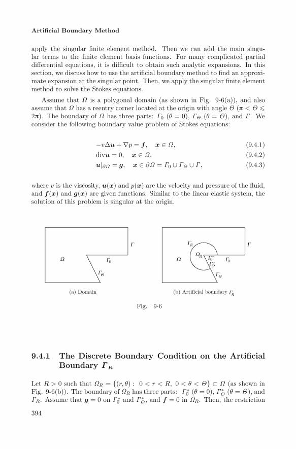
Assume that Ω is a polygonal domain (as shown in Fig. 9-6(a)), and alsoassume that Ω has a reentry corner located at the origin with angle Θ (π < Θ �2π). The boundary of Ω has three parts: Γ0 (θ = 0), ΓΘ (θ = Θ), and Γ . Weconsider the following boundary value problem of Stokes equations:

−vΔu + ∇p = f , x ∈ Ω , (9.4.1)divu = 0, x ∈ Ω , (9.4.2)u|∂Ω = g, x ∈ ∂Ω = Γ0 ∪ ΓΘ ∪ Γ , (9.4.3)

where v is the viscosity, u(x) and p(x) are the velocity and pressure of the fluid,and f(x) and g(x) are given functions. Similar to the linear elastic system, thesolution of this problem is singular at the origin.

Fig. 9-6

9.4.1 The Discrete Boundary Condition on the ArtificialBoundary ΓR

Let R > 0 such that ΩR = {(r, θ) : 0 < r < R, 0 < θ < Θ} ⊂ Ω (as shown inFig. 9-6(b)). The boundary of ΩR has three parts: Γ ∗

0 (θ = 0), Γ ∗Θ (θ = Θ), and

ΓR. Assume that g = 0 on Γ ∗0 and Γ ∗

Θ , and f = 0 in ΩR. Then, the restriction

394


on ΩR of the solution of (9.4.1)∼(9.4.3) satisfies

−v

(1r∂r (r∂rur) +

1r2

∂2θur − 2

1r2

∂θuθ − 1r2

ur

)+ ∂rp = 0,

(r, θ) ∈ ΩR, (9.4.4)

−v

(1r∂r (r∂ruθ) +

1r2

∂2θuθ + 2

1r2

∂θur − 1r2

uθ

)+

1r∂θp = 0,

(r, θ) ∈ ΩR, (9.4.5)

∂rur +1r∂θuθ +

1rur = 0, (r, θ) ∈ ΩR, (9.4.6)

ur|Γ∗0

= ur|Γ∗Θ

= 0, uθ|Γ∗0

= uθ|Γ∗Θ

= 0, (9.4.7)

where ur and uθ are the components of u in the r and θ directions, and ∂r and

∂θ denote the partial derivatives∂

∂rand

∂

∂θ, respectively. Let

V ={v : v ∈ H1((0,Θ)), v|θ=0 = v|θ=Θ = 0

},

M ={p(r, θ) : ∀r, p ∈ L2((0,Θ))

},

U ={u(r, θ) : ∀r, u, ∂ru, ∂2

ru ∈ V}

.

Then, problem (9.4.4)∼(9.4.7) is equivalent to the following differential-variationalproblem:⎧⎪⎪⎪⎪⎪⎪⎪⎪⎪⎪⎪⎪⎪⎪⎪⎪⎪⎪⎪⎪⎪⎨⎪⎪⎪⎪⎪⎪⎪⎪⎪⎪⎪⎪⎪⎪⎪⎪⎪⎪⎪⎪⎪⎩

Find ur ∈ U, uθ ∈ U, p ∈ M such that

−v

(1r∂r

(r∂r

∫ Θ

0

urvrdθ

)− 1

r2

∫ Θ

0

∂θur∂θvrdθ − 2r2

∫ Θ

0

∂θuθvrdθ

− 1r2

∫ Θ

0

urvrdθ

)+ ∂r

∫ Θ

0

pvrdθ = 0, ∀vr ∈ V,

−v

(1r∂r

(r∂r

∫ Θ

0

uθvθdθ

)− 1

r2

∫ Θ

0

∂θuθ∂θvθdθ +2r2

∫ Θ

0

∂θurvθdθ

− 1r2

∫ Θ

0

uθvθdθ

)− 1

r

∫ Θ

0

p∂θvθdθ = 0, ∀vθ ∈ V,

∂r

∫ Θ

0

urqdθ +1r

∫ Θ

0

∂θuθqdθ +1r

∫ Θ

0

urqdθ = 0, ∀q ∈ L2((0,Θ)).

(9.4.8)

We consider a semi-discrete approximation of problem (9.4.8). Divide [0,Θ ]equally into m − 1 = (n + 1)/2 (n odd) subintervals with length h:

0 = θ0 < θ2 < θ4 < · · · < θn+1 = Θ ,

395


Assume that Vh ⊂ V and Lh ⊂ L2((0,Θ)) are finite element subspaces:

Vh = {vh : vh ∈ V, vh|[θ2(j−1),θ2j ]

is a quadratic function of θ, j = 1, 2, · · · , m − 1},Lh = {qh : qh ∈ C((0,Θ)), qh|[θ2(j−1),θ2j]

is a linear function of θ, j = 1, 2, · · · , m − 1},

and ψi(θ), i = 1, 2, · · · , n, are basis functions of Vh satisfying

ψi(θj) ={

1, j = i,0, others, i = 1, 2, · · · , n, j = 0, 1, · · · , n + 1.

For vhr ∈ Vh and vh

θ ∈ Vh we have

vhr = ψ(θ)Tvh

r , vhθ = ψ(θ)Tvh

θ ,

where

ψ(θ) = (ψ1(θ), ψ2(θ), · · · , ψn(θ))T ,

vhr =

(vh

r,1, vhr,2, · · · , vh

r,n

)T, vh

θ =(vh

θ,1, vhθ,2, · · · , vh

θ,n

)T.

Denote the basis function of Lh by φi(θ), i = 1, 2, · · · , m, where φi(θ) satisfies

φi(θ2(j−1)) ={

1, i = j,0, others, i = 1, 2, · · · , m, j = 1, 2, · · · , m.

Then, for qh ∈ Lh we have

qh = φ(θ)Tqh

where

φ(θ) = (φ1(θ), φ2(θ), · · · , φm(θ))T , qh = (qh,1, qh,2, · · · , qh,m)T .

Let

Uh ={uh(r, θ) : uh, ∂ruh, ∂2

ruh ∈ Vh, ∀r}

,

Mh = {wh(r, θ) : wh ∈ Lh, ∀r} .

396


We consider the finite element approximation of problem (9.4.8):⎧⎪⎪⎪⎪⎪⎪⎪⎪⎪⎪⎪⎪⎪⎪⎪⎪⎪⎪⎪⎪⎪⎨⎪⎪⎪⎪⎪⎪⎪⎪⎪⎪⎪⎪⎪⎪⎪⎪⎪⎪⎪⎪⎪⎩

Find uhr ∈ Uh, uh

θ ∈ Uh, ph ∈ Mh such that

−v

(1r∂r

(r∂r

∫ Θ

0

uhrvh

r dθ

)− 1

r2

∫ Θ

0

∂θuhr ∂θv

hr dθ− 2

r2

∫ Θ

0

∂θuhθvh

r dθ

− 1r2

∫ Θ

0

uhr vh

r dθ

)+ ∂r

∫ Θ

0

phvhr dθ = 0, ∀vh

r ∈ Vh,

−v

(1r∂r

(r∂r

∫ Θ

0

uhθvh

θ dθ

)− 1

r2

∫ Θ

0

∂θuhθ∂θv

hθ dθ+

2r2

∫ Θ

0

∂θuhrvh

θ dθ

− 1r2

∫ Θ

0

uhθvh

θ dθ

)− 1

r

∫ Θ

0

ph∂θvhθ dθ = 0, ∀vh

θ ∈ Vh,

∂r

∫ Θ

0

uhr qhdθ +

1r

∫ Θ

0

∂θuhθqhdθ +

1r

∫ Θ

0

uhr qhdθ = 0, ∀qh ∈ Lh.

(9.4.9)

Letuh

r = ψ(θ)Tuhr (r), uh

θ = ψ(θ)Tuhθ (r), ph = φ(θ)Tph(r),

where

uhr (r) =

(uh

r,1(r), uhr,2(r), · · · , uh

r,n(r))T

,

uhθ (r) =

(uh

θ,1(r), uhθ,2(r), · · · , uh

θ,n(r))T

,

ph(r) = (ph,1(r), ph,2(r), · · · , ph,m(r))T .

Then, problem (9.4.9) is equivalent to the following boundary value problem ofordinary differential equations:

−v

(A

r∂r

(r∂ru

hr

)− (A + B)r2

uhr − 2C

r2uh

θ

)+ D∂rph = 0, (9.4.10)

−v

(A

r∂r

(r∂ru

hθ

)− (A + B)r2

uhθ − 2CT

r2uh

r

)− E

rph = 0, (9.4.11)

DT∂ruhr +

DT

ruh

r +ET

ruh

θ = 0, (9.4.12)

where A, B, and C are n × n matrices:

A =∫ Θ

0

ψ(θ)ψ(θ)Tdθ, B =∫ Θ

0

ψ′(θ)ψ′(θ)Tdθ,

C =∫ Θ

0

ψ(θ)ψ′(θ)Tdθ;

397


D and E are n × m matrices:

D =∫ Θ

0

ψ(θ)φ(θ)Tdθ, E =∫ Θ

0

ψ′(θ)φ(θ)Tdθ.

Introduce the change of variable r = es. Then (9.4.10)∼(9.4.12) becomes

−v(A∂2

s uhr − (A + B)uh

r − 2Cuhθ

)+ esD∂sph = 0,

−v(A∂2

s uhθ − (A + B)uh

θ − 2CTuhr

)− esEph = 0,

DT∂suhr + DTuh

r + ETuhθ = 0.

Letph = rph, wh

r = ∂suhr , wh

θ = ∂suhθ .

Then, we have

−v(A∂sw

hr − (A + B)uh

r − 2Cuhθ

)+ D∂sph − Dph = 0,

−v(A∂sw

hθ − (A + B)uh

θ − 2CTuhr

)− Eph = 0,

DTwhr + DTuh

r + ETuhθ = 0.

In matrix form, we have[A11 A12

0 0

] [∂sUh

∂sph

]=[

B11 B12

B21 0

] [Uh

ph

], (9.4.13)

where

A11 =

⎡⎢⎢⎣vA 0 0 00 I 0 00 0 vA 00 0 0 I

⎤⎥⎥⎦ , A12 =

⎡⎢⎢⎣−D000

⎤⎥⎥⎦ ,

B11 =

⎡⎢⎢⎣0 v(A + B) 0 2vCI 0 0 00 2vCT 0 v(A + B)0 0 I 0

⎤⎥⎥⎦ , B12 =

⎡⎢⎢⎣−D0

−E0

⎤⎥⎥⎦ ,

B21 =[DT DT 0 ET

], Uh =

[wh

r uhr wh

θ uhθ

]T.

Using the RQ decomposition, we have[B11 B12

B21 0

]= RQ =

[R11 R12

0 R22

] [Q11 Q12

Q21 Q22

],

where R is upper triangular and Q is orthogonal. From (9.4.13), we obtain[A11 A12

0 0

] [QT

11 QT21

QT12 QT

22

] [∂sU

∗h

∂sp∗h

]=[

R11 R12

0 R22

] [U∗

h

p∗h

], (9.4.14)

398


or [A11Q

T11 + A12Q

T12 A11Q

T21 + A12Q

T22

0 0

] [∂sU

∗h

∂sp∗h

]=[

R11 R12

0 R22

] [U∗

h

p∗h

],

where [U∗

h

p∗h

]= Q

[Uh

ph

]. (9.4.15)

For the RQ decomposition, we haveLemma 9.4.1 The matrix [

B11 B12

B21 0

]is nonsingular, and consequently R11 and R22 are both nonsingular.Proof. We only need to show that the linear system⎡⎢⎢⎢⎢⎣

0 v(A + B) 0 2vC −DI 0 0 0 00 2vC 0 v(A + B) −E0 0 I 0 0

DT DT 0 ET 0

⎤⎥⎥⎥⎥⎦⎡⎢⎢⎢⎢⎣

wr

ur

wθ

uθ

p

⎤⎥⎥⎥⎥⎦ = 0

has only zero solution. Since wr = wθ = 0, we have

v(A + B)ur + 2vCuθ − Dp = 0, (9.4.16)2vCTur + v(A + B)uθ − Ep = 0, (9.4.17)DTur + ETuθ = 0. (9.4.18)

From (9.4.16) and (9.4.17), we obtain[ur

uθ

]= v

[A + B 2C2CT A + B

]−1 [DpEp

]. (9.4.19)

Substituting this into (9.4.18), we get

v[

DT ET] [ A + B 2C

2CT A + B

]−1 [DE

]p = 0.

Multiplying both sides by p, we find

v[

(Dp)T (Ep)T]K−1

[DpEp

]= 0,

where

K =[

A + B 2C2CT A + B

].

399


The matrix K can be viewed as the stiffness matrix obtained from the quadraticfinite element approximation to the following system of ordinary differentialequations:

−u′′ + v′ + u = 0,

−v′′ − u′ + v = 0,

u(0) = u(Θ) = v(0) = v(Θ) = 0,

Thus, K is positive definite. Then, we have[DpEp

]= 0.

A direct calculation shows that the rank of D is m, and hence p = 0 is theunique solution. Substituting into (9.4.19), we get ur = 0, uθ = 0.

From (9.4.14), we haveR22p

∗h = 0,

Using Lemma 9.4.1, we obtain

p∗h = 0, ∂sp

∗h = 0. (9.4.20)

Then, the first equation of (9.4.14) is simplified as

(A11QT11 + A12Q

T12)∂sU

∗h = R11U

∗h (9.4.21)

We look for the solution of the following form:

U∗h = eσsζ.

Substituting into (9.4.21), we arrive at the following eigenvalue problem:

R−111 (A11Q

T11 + A12Q

T12)ζ = λζ, (9.4.22)

where λ = 1/σ.

Lemma 9.4.2 (i) The eigenvalue problem (9.4.22) has no eigenvalues of theform αi, where α is any real number and i =

√−1; (ii) If λ is an eigenvalue of(9.4.22), then −λ is also an eigenvalue of (9.4.22).

Proof. (9.4.22) can be rewritten as[A11 A12

0 0

] [QT

11 QT21

QT12 QT

22

] [ζ0

]= λ

[R11 R12

0 R22

] [ζ0

],

or equivalently,[A11 A12

0 0

] [QT

11ζQT

12ζ

]= λ

[B11 B12

B21 0

] [QT

11ζQT

12ζ

].

400


Let [ξr ξr ξθ ξθ η

]T=[

QT11ζ

QT12ζ

]=[

QT11 QT

21

QT12 QT

22

] [ζ0

].

Then, ⎡⎢⎢⎢⎢⎣vA 0 0 0 −D0 I 0 0 00 0 vA 0 00 0 0 I 00 0 0 0 0

⎤⎥⎥⎥⎥⎦⎡⎢⎢⎢⎢⎣

ξr

ξr

ξθ

ξθ

η

⎤⎥⎥⎥⎥⎦

= λ

⎡⎢⎢⎢⎢⎣0 v(A + B) 0 2vC −DI 0 0 0 00 2vC 0 v(A + B) −E0 0 I 0 0

DT DT 0 ET 0

⎤⎥⎥⎥⎥⎦⎡⎢⎢⎢⎢⎣

ξr

ξr

ξθ

ξθ

η

⎤⎥⎥⎥⎥⎦ .

In the above equations, we have

vAξr − Dη = λv(A + B)ξr + 2λvCξθ − λDη,

ξr = λξr ,

vAξθ = 2λvCTξr + λv(A + B)ξθ − λEη,

ξθ = λξθ,

DTξr + DTξr + ETξθ = 0,

or,

ξr = λξr , ξθ = λξθ ,

G(λ)ζ = 0,

where

G(λ) =

⎡⎣ v(λ2(A + B) − A

)2vλ2C (1 − λ)D

2vλ2CT v(λ2(A + B) − A

) −λE(1 + λ)DT λET 0

⎤⎦ ,

ζ =

⎡⎣ ξr

ξθ

η

⎤⎦ .

For any real number α,

G(αi) =

⎡⎣ −v(α2(A + B) + A

) −2vα2C (1 − αi)D−2vα2CT −v

(α2(A + B) + A

) −αiE(1 + αi)DT αiET 0

⎤⎦ .

401


Let

G(αi)

⎡⎣ ξr

ξθ

η

⎤⎦ = 0,

or,

K1

[ξr

ξθ

]=[

(1 − αi)Dη−αiEη

],[

(1 + αi)DT αiET] [ ξr

ξθ

]= 0,

where

K1 =[

v(α2(A + B) + A

)2vα2C

2vα2CT v(α2(A + B) + A

) ]= vα2K + v

[A 00 A

].

Obviously, A is symmetric and positive definite, and hence K1 is also symmetricand positive definite. Then, we have

[(1 + αi)DT αiET

]K−1

1

[(1 − αi)Dη−αiEη

]= 0.

Multiplying the above equation by η, and let

η∗ =[

(1 − αi)Dη−αiEη

],

we obtain(η∗)TK−1

1 η∗ = 0,

where η∗ is the conjugate of η∗. Notice that K−11 is also symmetric and positive

definite; thus η∗ = 0. Using this and notice that the rank of D is m, we getη = 0. Therefore, ξr = ξθ = 0, G(αi) is singular, and αi is not an eigenvalue of(9.4.22). Finally, it is easy to check that G(−λ) = GT(λ). Therefore, if λ is aneigenvalue, then det (G(−λ)) = det

(GT(λ)

)= det (G(λ)) = 0, i.e., −λ is also

an eigenvalue.It is easy to see from the proof of Lemma 9.4.2 that R−1

11 (A11QT11 + A12Q

T12)

has no zero eigenvalue. Then, (9.4.22) can be rewritten as

(A11QT11 + A12Q

T12)

−1R11ζ = σζ (9.4.23)

where σ =1λ

, and we have the following theorem:

Theorem 9.4.1 The eigenvalue problem (9.4.22) has 2n eigenvalues σ1, σ2, · · · ,σ2n with positive real parts, and 2n corresponding eigenvalues: −σ1, −σ2, · · · ,−σ2n.

402


Assume that uhr (r) and uh

θ (r) are bounded as r → 0. Then, from Theorem9.4.1 we get the solution of (9.4.14):

U∗h =

2n∑j=1

cjeσjsζj .

The solution of problem (9.4.13) is

[Uh

ph

]=

2n∑j=1

cjrσj QT

[ζj

0

],

where r = es. Setting

QT[ζj , 0]T =[ξr,j ξr,j ξθ,j ξθ,j ηj

]T,

we may write ⎡⎣ uhr

uhθ

ph

⎤⎦ =2n∑

j=1

cjrσj

⎡⎣ ξr,j

ξθ,j

ηj

⎤⎦ .

The solution of problem (9.4.9) is

uhr (r, θ) =

2n∑j=1

cjrσj ψ(θ)Tξr,j , (9.4.24)

uhθ (r, θ) =

2n∑j=1

cjrσj ψ(θ)Tξθ,j , (9.4.25)

ph(r, θ) =2n∑

j=1

cjrσj−1φ(θ)Tηj. (9.4.26)

Equations (9.4.24)∼(9.4.26) are the discrete form of the asymptotic expan-sion near the singular point for the solution of the Stokes equations (9.4.1)∼(9.4.3).

9.4.2 Singular Finite Element Approximation

Using the asymptotic expansion (9.4.24)∼(9.4.26) near the singular point, weconsider the singular finite element approximation of (9.4.1)∼(9.4.3). We firstintroduce the following index sets:

Nr = {j : 1 � j � 2n, σj is real.},Nc = {j : 1 � j � 2n, σj = aj + bji, bj > 0}.

403


Then, the real solution corresponding to (9.4.24)∼(9.4.26) is

uhr (r, θ)=

∑j∈Nr

cjrσj ψ(θ)Tξr,j

+∑

j∈Nc

cjraj ψ(θ)T

(ξ∗

r,j cos(bj ln r) − ξ′r,j sin(bj ln r)

)+∑

j∈Nc

djraj ψ(θ)T

(ξ∗

r,j sin(bj ln r) + ξ′r,j cos(bj ln r)

),

uhθ (r, θ)=

∑j∈Nr

cjrσj ψ(θ)Tξθ,j

+∑

j∈Nc

cjraj ψ(θ)T

(ξ∗

θ,j cos(bj ln r) − ξ′θ,j sin(bj ln r)

)+∑

j∈Nc

djraj ψ(θ)T

(ξ∗

θ,j sin(bj ln r) + ξ′θ,j cos(bj ln r)

),

ph(r, θ)=∑

j∈Nr

cjrσj−1φ(θ)Tηj

+∑

j∈Nc

cjraj−1φ(θ)T

(η∗

j cos(bj ln r) − η′j sin(bj ln r)

)+∑

j∈Nc

djraj−1φ(θ)T

(η∗

j sin(bj ln r) + η′j cos(bj ln r)

),

where [ξ∗r,j , ξ

∗r,j , ξ

∗θ,j, ξ

∗θ,j, η

∗j ]T and [ξ′

r,j , ξ′r,j , ξ

′θ,j, ξ

′θ,j , η

′j]

T are the real and imag-inary parts of QT[ζj , 0]T. Then,

u≈∑

j∈Nr

cjrσj f

(0)j (θ)

+∑j∈Nc

cjraj

(f

(1)j (θ) cos(bj ln r) − f

(2)j (θ) sin(bj ln r)

)+∑j∈Nc

djraj

(f

(1)j (θ) sin(bj ln r) + f

(2)j (θ) cos(bj ln r)

), (9.4.27)

p≈∑

j∈Nr

cjrσj−1g

(0)j (θ)

+∑j∈Nc

cjraj−1

(g(1)j (θ) cos(bj ln r) − g

(2)j (θ) sin(bj ln r)

)+∑j∈Nc

djraj−1

(g(1)j (θ) sin(bj ln r) + g

(2)j (θ) cos(bj ln r)

), (9.4.28)

404


where u = (u1, u2)T,

f(0)j (θ) = T

[ψ(θ)Tξr,j

ψ(θ)Tξθ,j

], T =

[cos θ − sin θsin θ cos θ

],

f(1)j (θ) = T

[ψ(θ)Tξ∗

r,j

ψ(θ)Tξ∗θ,j

], f

(2)j (θ) = T

[ψ(θ)Tξ′

r,j

ψ(θ)Tξ′θ,j

],

g(0)j (θ) = φ(θ)Tηj , g

(1)j (θ) = φ(θ)Tη∗

j , g(2)j (θ) = φ(θ)Tη′

j .

In (9.4.27)∼(9.4.28), take σj and ak such that σj , ak ∈ (0, 2], and assume thatthey form the sets {σj}M1

1 and {ak}M21 . We construct the following singular

finite element spaces:

Sh1 =Span{η(r, θ)rσj f

(0)j (θ),

η(r, θ)rak (f (1)k (θ) cos(bk ln r) − f

(2)k (θ) sin(bk ln r)),

η(r, θ)rak (f (1)k (θ) sin(bk ln r) + f

(2)k (θ) cos(bk ln r)),

j = 1, · · · , M1; k = 1, 2, · · · , M2},Qh

1 =Span{rσj−1g(0)j (θ),

rak−1(g(1)k (θ) cos(bk ln r) − g

(2)k (θ) sin(bk ln r)),

rak−1(g(1)k (θ) sin(bk ln r) + g

(2)k (θ) cos(bk ln r)),

j = 1, 2, · · · , M1; k = 1, 2, · · · , M2},where η(r, θ) is any truncation function with 1 at the origin and 0 on the bound-ary ∂Ω . Let

Uh = {uh(x) : uh(x) ∈ Sh0 ⊕ Sh

1 , uh(xs) = g(xs), ∀s ∈ Nb},Vh = {vh(x) : vh(x) ∈ Sh

0 ⊕ Sh1 , vh(xs) = 0, ∀s ∈ Nb} ⊂ (H1

0 (Ω))2

,

Mh =(Qh

0 ⊕ Qh1

) ∩ L20(Ω)

where

Sh0 ={v(x) ∈ C(Ω) : v|K is a quadratic polynomial.}

Qh0 ={q(x) ∈ C(Ω) : q|K is a linear polynomial.}

is the standard finite element space. Thus, we get the singular finite elementapproximation for the Stokes equations (9.4.1)∼(9.4.3):⎧⎨⎩

Find (uh(x), ph(x)) ∈ Uh × Mh such thata(uh, vh) − b(vh, ph) = (f , vh), ∀vh ∈ Vh,b(uh, wh) = 0, ∀wh ∈ Mh,

(9.4.29)

where

a(uh, vh) = v

∫Ω

∇uh∇vhdxdy, b(uh, wh) =∫Ω

whdiv uhdxdy.

405


The main references for this chapter are: Wu and Han (1997); Wu and Han(2001); Wu and Xue (2003); Wu and Cheung (1999); and Wu and Jin (2005).For related works on the artificial boundary method for boundary value problemand interface face problem of the second-order elliptic equations, we refer thereaders to Han (1982); Yu (1983-B); Han and Huang (1999-A). For related workson the computation of the stress intensity factors in various problems of fracturemechanic of linear elasticity, we refer the readers to Babuska and Oh (1990);Babuska and Rosenzweig (1972); Fix, Gulati, and Wakoff (1973); Givoli andRivkin (1993); Givoli and Vigdergauz (1994); Guo and Oh (1994); Kellogg (1971,1975); Li, Mathon and Sermer (1987); Han and Huang (1999-B); Han, Huang,and Bao (2000); Bao, Han, and Huang (2001);Han and Huang (2001-A); andTsamasphyros (1987).

References

[1] Anderson, T.L. (1995), Fracture Mechanics: Fundamentals and Applica-tions. (2nd ed.). CRC Press, Boca Raton, 1995.

[2] Babuska, I. and Oh, H.S. (1990), The p-version of the finite element methodfor domains with corners and for infinite domains, Numer. Meth. PDEs,6(1990), 371-392.

[3] Babuska, I. and Rosenzweig, M.R. (1972), A finite element scheme fordomains with corners, Numer. Math., 20(1972), 1-21.

[4] Bao, W.Z., Han, H.D. and Huang, Z.Y. (2001), Numerical simulationsof fracture problems by coupling the FEM and the direct method of lines,Comput. Methods Appl. Mech. Engrg., 190 (2001), 4831-4846.

[5] Ciarlet, P.G. (1977), The Finite Element Method for Elliptic Problems,North-Holland, 1977.

[6] Fix, G., Gulati, S. and Wakoff, G.I. (1973), On the use of singular functionswith the finite element method, J. Comput. Phys., 13 (1973), 209-228.

[7] Givoli, D. and Rivkin, L. (1993), The DtN finite element method for elasticdomains with cracks and re-entrant corners, Computers & Structures, 49(1993), 633-642.

[8] Givoli, D. and Vigdergauz, S. (1994), Finite element analysis of wave scat-tering from singularities, Wave Motion, 20 (1994), 165-176.

[9] Guo, B. and Oh, H.S. (1994), The h-p version of the finite element methodfor problems with interfaces, Inter. J. Numer. Meth. Eng., 37 (1994),1741-1762.

406


[10] Han, H.D. (1982), The numerical solutions of interface problems by infiniteelement method. Numer. Math., 39 (1982), 39-50.

[11] Han, H.D. and Huang, Z.Y. (1999-A), The direct method of lines for thenumerical solutions of interface problem, Comput. Meth. Appl. Mech.Engrg., 171 (1999), 61-75.

[12] Han, H.D. and Huang, Z.Y. (1999-B), A semi-discrete numerical procedurefor composite material problems, Math. Sci. Appl., 12 (1999), Adv. numer.math., 35-44.

[13] Han, H.D. and Huang, Z.Y. (2001-A), The discrete method of separationof variables for composite material problems, Int. J. Fracture, 112 (2001)379-402.

[14] Han, H.D., Huang, Z.Y. and Bao, W.Z. (2000), The discrete method ofseparation of variables for computation of stress intensity factors, ChineseJ. Comput. Phy., 17 (2000), 483-496.

[15] Karp, S.N. and Karal, F.C. Jr. (1962), The elastic-field behaviour in theneighbourhood of a crack of arbitrary angle, Comm. Pure Appl. Math., 15(1962), 413-421.

[16] Kellogg, R.B. (1971), singularities in interface problems, in: B. Huffard,ed., Numerical Solution of Partial Differential Equations 2 (AcademicPress, New York, 1971).

[17] Kellogg, R.B. (1975), On the Poisson equation with intersecting interfaces,Appl. Anal., 4 (1975), 101-129.

[18] Li, Z.C., Mathon, R. and Sermer, P. (1987), Boundary method for solv-ing elliptic problems with singularities and interfaces, SIAM J. of Numer.Anal. 24 (1987), 487-498.

[19] Lions, P.L. (1988), On the Schwarz alternating method I, First interna-tional symposium on domain decomposition methods for partial differen-tial equations proceedings, 1-42, SIAM, Philadelphia, 1988.

[20] Tsamasphyros, G. (1987), Singular element construction using a mappingtechnique, Inter. J. Numer. Meth. Eng., 24 (1987), 1305-1316.

[21] Wu, X.N. and Cheung, C.Y. (1999), An iteration method using artificialboundary for some elliptic boundary value problems with singularities, Int.J. Numer. Meth. Engng., 46 (1999), 1917-1931.

[22] Wu, X.N. and Han, H.D. (1997), A finite-element method for Laplace andHelmholtz type boundary value problems with singularities, SIAM, J. Nu-mer. Anal.,Vol.34 (1997), 1037-1050.

407


[23] Wu, X.N. and Han, H.D. (2001), Discrete boundary conditions for problemswith interface, Comput. Meth. Appl. Mech. Engrg., 190 (2001), 4987-4998.

[24] Wu, X.N. and Jin, J.C. (2005), A finite element method for Stokes equa-tions using discrete singularity expansion, Comput. Meth. Appl. Mech.Eng., 194(2005), 83-101.

[25] Wu, X.N. and Xue, W.M. (2003), Discrete boundary conditions for elas-ticity problems with singularities, Comput. Meth. Appl. Mech. Engrg.,192 (2003), 3777-3795.

[26] Yu, D.H. (1983-B), Coupling canonical boundary element metdod with FEMto solve harmonic problem over cracked domain, J. Comp. Math., 1(1983),195-202.

[27] Yu, D.H. (1994-A), A domain decomposition method based on naturalboundary reduction over unbounded domain, Math. Numer. Sinica 16(1994), 448-459.

408

artificial boundary method || applications to problems with singularity

Documents