article rule-based demand side management of domestic … · this saturation is often ......

May 3, 2013 12:20 Journal of Building Performance Simulation JBPS˙Paper˙AAM

Journal of Building Performance SimulationVol. xx, No. xx, xx xx, 1–27

Article

Rule-based demand side management of domestic hot water production with

heat pumps in zero energy neighbourhoods

R. De Conincka,b∗, R. Baetensc, D. Saelensc, A. Woyteb and L. Helsena

aApplied Mechanics and Energy Conversion, Department of Mechanical Engineering, KU Leuven,

Belgium; b3E, Brussels, Belgium; cBuilding Physics Section, Department of Civil Engineering, KU

Leuven, Belgium;

(Accepted version of May 3, 2013)

Grid saturation has been reported in electricity distribution systems with a high penetration of photovoltaic(PV) systems. This saturation is often caused by overvoltage and results in curtailing or shutting-down of thePV inverters, leading to a loss of renewable electricity generation.

The presented work assesses the potential of rule-based demand side management (DSM) applied to domestichot water (DHW) production with heat pumps in dwellings for reducing the non-renewable energy use of theneighbourhood.

The studied case consists of 33 single-family dwellings connected to the IEEE 34 node test feeder in amoderate European climate. Each dwelling is designed as a net zero energy building (NZEB) by adequatedesign of a heat pump and PV system.

A detailed dynamic simulation model is implemented by use of a cross domain Modelica library for integrateddistrict energy assessment. The user behaviour is obtained from a stochastic model based on Markov chainsand survival analysis. Different rule-based DSM control strategies are applied to the individual dwelling’s DHWsystems.

The results show that for balancing the PV production, active thermal energy storage in the DHW storagetanks is very promising. Even with very basic control algorithms and small storage tanks of 0.3 m3, curtailinglosses can be reduced by 74 %. This represents a net energy saving on neighbourhood level of 3.4 %.

Keywords: demand side management (DSM), rule-based control, photovoltaics (PV), Modelica, thermalenergy storage (TES), integrated neighbourhood simulation

Acknowledgment (AAM)

This is an Author’s Accepted Manuscript (AAM) of an article accepted for publication by theJournal of Building Performance Simulation [copyright Taylor & Francis]. This article includesmodifications as a result of the peer review process organised by the publisher. The Journalof Building Performance Simulation is available online at http://www.tandfonline.com/loi/

tbps20.

1. Introduction

1.1 Grid saturation due to overvoltage

Distributed electricity generation (DG) affects the operating conditions of distribution grids indifferent ways (Dugan and McDermott, 2001; Ackermann and Knyazkin, 2002). One specific

∗Corresponding author. Email: [email protected]

ISSN: 1940-1493 print/ISSN 1940-1507 onlinec© xx Taylor & FrancisDOI: 10.1080/1940149YYxxxxxxxxhttp://www.informaworld.com

http://www.tandfonline.com/loi/tbps20

http://www.tandfonline.com/loi/tbps20


2 Roel De Coninck, Ruben Baetens, Dirk Saelens, Achim Woyte, Lieve Helsen

issue consists of steady-state voltage rises, which are of particular interest in distribution gridswith a large amount of PV systems (Woyte et al., 2006; Caamano Martin et al., 2008). Attimes of high solar radiation, these voltage rises may result in a shut down of some of the PVinverters, or a curtailing of the output power by droop control (De Brabandere et al., 2004).These problems will happen more frequently as the cumulative installed PV capacity is expectedto keep on rising in existing distribution grids (EPIA, 2012).

As a result of the European policy regarding building energy performance, low energy neigh-bourhoods will have to become the standard for new construction from 2020 onwards (EuropeanParliament, 2010). In these low energy buildings and neighbourhoods, PV and heat pump tech-nology are often combined in order to reach a yearly ’net zero’ energy balance. However, thismay lead to inverter shut down or droop control at certain times, causing a loss of renewableelectricity generation. For example, Baetens et al. (2012) computed a loss of 14 % to 47 % of theexpected local PV electricity generation in a low energy neighbourhood, depending on feedersizing and parameter settings for the overvoltage shut-down.

Possible solutions to reduce the amount of curtailed power in distribution grids with a largeamount of PV systems consist of:

• Feeder reinforcements

• Changing the transformer tap positions to obtain an adapted voltage at the point of commoncoupling

• Active voltage control with modern inverters (Bletterie et al., 2010)

• Demand side management (DSM)

This paper assesses the potential of rule based DSM applied to the domestic hot water (DHW)production in dwellings with heat pumps. The aim of load shifting is not the voltage control onitself, but a reduction of the non-renewable energy use of the neighbourhood.

1.2 Demand side management

The idea of DSM for this case is straightforward: by shifting electrical loads to time periodsof excessive voltage in the grid, curtailing of the inverters can be avoided. There are differentoptions for the shiftable loads. This paper will neither consider load shifting with householdappliances like dishwashers, cloth washers and dryers, nor by use of an electrical battery.

The shiftable load is the compression heat pump that produces heat for space heating andDHW. This paper only considers the DHW production as a shiftable load. The required flexibilityto enable the decoupling of heat generation and consumption is the thermal energy storage (TES)tank for storage of the domestic hot water. We only consider DHW and exclude space heatingfrom this paper because the latter requires a more detailed analysis in order to cover the differentemission systems and control strategies which lies beyond the scope of this paper. As will beshown, the potential of load shifting on DHW is substantial and justifies the current scope. Theapplication of the elaborated methodology on space heating is a topic for future work.

In a previous study, different control strategies had been applied to a heat pump for spaceheating in a single dwelling (De Coninck et al., 2010). Although it was shown that peak loadscan be reduced at the level of an individual building, the impact of these control strategies onthe distribution grid and consequently the inverter behaviour could not be assessed. This papertakes the next step by modelling the entire neighbourhood.

1.3 Modelling of neighbourhoods

Simulations or optimizations on a single building level cannot be used to study the operationof the distribution grid. DSM studies on single buildings can be used to study the energy orcost savings in that building, up to the power exchange with the grid. It is however incorrect touse these studies for drawing conclusions about the ability of DSM to compensate for stochastic


Journal of Building Performance Simulation 3

electricity generation or distribution grid loads. For this purpose, a neighbourhood model isrequired, composed of the distribution grid, different buildings and stochastic user behaviour.

On the other hand, neighbourhood (or district) level simulations are not new. Manfren et al.(2011) discuss different aspects of district level simulations whereas Baetens et al. (2012) givea good overview of existing approaches and tools.

DSM applied to heat pumps has to be studied with detailed dynamic models. These mod-els need to include the building, heating, ventilation and air-conditioning (HVAC) and userbehaviour. This is required for capturing the interaction between the heating system and thebuilding, the effects of ambient, inside and TES tank temperatures on the heat pump efficiency,the consequences of on/off cycling, etc. Most district simulation tools cannot cope with the de-sired level of detail in the building model. On the other hand, typical building simulation toolsdo not allow to model multiple buildings connected to a distribution grid. In order to combinethe best of two worlds, we use Modelica.

The present paper shows how thermal energy management can be applied in order to relievegrid saturation on neighbourhood level. Special attention is paid to the modelling of the DHWsystem because both the hot water demand and the TES tank model largely influence thepotential of DSM. Modelica has proven well suited for this purpose.

2. Model

2.1 Overview

The model consists of 33 single-family dwellings connected to the 34-node test feeder of theInstitue of Electrical and Electronics Engineers (IEEE) (Kersting, 2001) in the moderate Euro-pean climate of Uccle, Belgium. It is assumed that all dwellings are identical, built according toa low-energy standard, heated with a modulating air-to-water heat pump and equipped with aPV system covering their complete yearly energy needs. The following paragraphs elaborate onthe modelling principles and details, whereas Tables 1 and 2 give an overview of the buildingand general model parameters respectively.

2.2 Dwelling

A single dwelling typology is used which was identified in the European TABULA project (Logaet al., 2009) as representative for semi-detached single-family houses constructed after the year2005. This means that all dwellings are identical and that the variation in temperature and loadis caused entirely by the stochastic user behaviour. The dwelling has a total heated floor area of196 m2, a total volume of 643 m3, a compactness of 1.58 m and is modelled as a single thermalzone. The dwelling is designed according to a low-energy standard and has massive walls andfloors. The composition of the different envelope elements and resulting U-values are given inTable 1.

We suppose an air-tightness corresponding to the low energy standard with a natural infil-tration rate of 0.03 air changes per hour (ACH). All dwellings are equipped with mechanicallybalanced, air-to-air heat-recovery ventilation with an air change rate of 0.5 ACH and a recoveryefficiency of 0.84.

All dwellings have exterior solar screens with a solar transmittance of 0.24. As a result noactive cooling needs to be installed in the dwellings. The automated exterior solar screen islowered at a global horizontal irradiation level of 250 W/m2 and raised again at an irradiationlevel below 150 W/m2.



Table 1. Overview of building model parameters

Element A U g(m2) (W/(m2 K)) (-)

Outer facade a 135.0 0.22 -Floor b 98.0 0.19 -Roof c 118.0 0.11 -Windows 33.5 1.10 0.59

a 15 cm of PUR between an 8 cm outer and 14 cminner brick wall.

b 10 cm of PUR below a 8 cm screed layer andon a 20 cm concrete slab.

c 30 cm of mineral wool between multiplex platesin a timber frame construction.

M

heat pump

pumpDHW pumpFH

cold water

mixing valve DHW

floor heating

(FH)DHW storage tank

mixing valve FH3-way valve DHW/FH

Figure 1. Hydraulic scheme of the heating and DHW system

2.3 HVAC system

Each of the 33 dwellings has an identical space heating and DHW system, visualized in Figure 1.Heat is produced by means of a modulating air-to-water heat pump (HP), connected to a floorheating and a DHW storage tank.

2.3.1 Heating

The heat pump model is based on linear interpolation in a performance map retrieved frommanufacturer data (Daikin Europe N.V., 2006). The performance map does not take into account(de)frosting of the evaporator as shown in Figure 2 (although it does extend to negative ambienttemperatures). The nominal coefficient of performance (COP) is 3.17 at 2/35 ◦C and 2.44 at2/45 ◦C test conditions (i.e. air/water temperature) for full load operation. The thermal powerof the heat pump is 3459 W at 2/35 ◦C.

The interpolation in the performance map defines the heating power Qnet (W) and electricityuse Pnet (W) as a function of condenser outlet temperature, the ambient temperature andmodulation level (between 25 % and 100 %). The heat pump can modulate thanks to an inverterat the compressor. In the model, the modulation level modfinal (%) is obtained in two steps.First, the initial modulation mod init (%) is computed according to Equation (1), and thenlimited according to Equation (2). To avoid on/off cycling, a hysteresis is added to the startingcondition: the heat pump will only start when mod init ≥ 50%.

mod init =Qdemand

Qmax

=mcp(Tset − Ti)

f(Tevap , Tc)(1)



Figure 2. Performance map of the heat pump, showing the COP as a function of ambient temperature for different modu-lation levels (30 %, 50 %, 90 % and 100 %) and different condenser outlet temperatures (30 ◦C, 40 ◦C and 50 ◦C).

modfinal =

0%(= off) if mod init < 25%,

100% if mod init ≥ 100%,

mod init else.

(2)

In these equations, m (kg/s) is the mass flow rate in the condenser, cp (J/(kg s)) the specificheat capacity of water, Tset (K) is the condenser set temperature, Ti (K) is the condenser inlettemperature, Qdemand (W) is the demanded thermal power and Qmax (W) is the maximumthermal power at the current evaporator temperature Tevap (K) and condenser temperature Tc

(K), obtained from the performance map.The model takes into account the water content of the condenser mc (kg) and dry capacity cdry

(J/K), both connected to the environmental temperature Te (K) through a thermal conductanceUAloss (W/K) in order to obtain a dynamic model with heat losses according to Equation (3).

(mccp + cdry)dTc

dt= mcp(Ti − Tc) + Q−UAloss(Tc − Te) (3)

In this equation, Q (W) is the condensation heat Qnet augmented with the environmental heatlosses UAloss(Tc−Te). This ensures that the steady state efficiency of the heat pump is identicalto the performance data, while adding environmental losses and dynamics to the model. Theproduced heat is used for charging the floor heating, designed to work at a 35/30 ◦C regime atdesign conditions and for charging the domestic hot water storage tank. As mentioned above,the investigated DSM controls only concern the charging of the DHW tank.



2.3.2 Domestic hot water and storage tank

The stratified water energy storage tank is only used for DHW production. It is connectedto the heat pump through an internal heat exchanger, and the hot water is withdrawn via athermostatic mixing valve in order to obtain water at 45 ◦C. A one-dimensional multinode storagetank model is used. For each node i (numbering starts at the top), the energy balance and massbalance equations are given in respectively Equations (4) and (5) and presented schematicallyin Figure 3.

micpdTidt

=∑j

cpmjTj + Qcond,i−1 + Qcond,i + Qbuo,i + Qbuo,i−1 + Qenv,i + QHX ,i (4)

∑j

mj = 0 (5)

In these equations, mi (kg) is the water mass of the node i with temperature Ti (K) and cp is thespecific heat of water, assumed to be constant and equal to 4177 J kg−1 K−1. The in- and outgoingwater flows in node i due to forced circulation are represented by mj (kg/s), their correspondingtemperatures by Tj (K) (for outgoing flows, Tj = Ti). Heat transfer to neighbouring nodes via

conduction is given by Qcond (W). Transmission losses to the environment are given by Qenv,i(W). When the node i contains a section of the internal heat exchanger, the heat transfer fromthis section into the node is given by QHX ,i (W). Qbuo (W) is the equivalent heat transfer toneighbouring nodes due to buoyancy effects and this term will be elaborated in the followingparagraphs. Mass flow rates and heat fluxes entering the node i have a positive sign.

Figure 3. Schematic overview of the nodal energy balance in the TES tank

The storage tank plays a key role in the DSM strategies, therefore specific attention was paidto verification and calibration of the model to manufacturer data. The goal of this calibrationis to obtain a robust model formulation, that can be used for different storage volumes. Thisrequires that the model parameters are independent of the size and geometry of the nodes.

Technical information and measurements from the commercial DHW tank Vitocell 100-V, typeCVW of 390 l are used to tune the parameters of the model (Viessmann, 2011).

Firstly, geometrical details like tank diameter and height, surface and water content of theinternal heat exchanger are set. The heat transfer coefficients of the internal heat exchanger(internal convection, conduction and external convection) are calculated based on heat transfercorrelations.

Secondly, the parameters for the transmission losses Qenv,i are set. In order to obtain a para-metric model that allows scaling, a fixed UAfix(W K−1) and a surface dependent heat losscoefficient UIns(W m−2 K−1) are defined. UIns depends on thickness and thermal conductivity



of the insulation. UAfix accounts for cold bridges and increased heat losses at the connectionsand is fixed to match the given 24 hour heat losses according to DIN V 18599.

Finally, the remaining parameters to be set are the number of layers and the buoyancy model,which are linked. The aim of this calibration exercise is to find a model with a relatively lownumber of layers that is robust to changes in storage volume. Therefore, the number of layers andthe buoyancy formulation should not influence the yearly performance of the storage tank (oronly to a limited extend). Thermal stratification and buoyancy are complex processes dependingon tank geometry and operation conditions. Haller et al. (2009) review different methods thathave been proposed to characterize thermal stratification in TES tanks. All attempts to includethese phenomena in one-dimensional stratified storage tank models are strong simplificationsof the 3-D flow patterns that occur (Han et al., 2009). Most one-dimensional stratified storagetank models approximate buoyancy effects as mixing between the layers in case of temperatureinversion (Zurigat et al., 1989). In case of a fixed time step simulation, the mixing rate dependson the node volume and simulation time step (Newton, 1995; Mather et al., 2002). In case ofcontinuous time solvers, a parameter is required for the time constant of mixing (Wetter, 2009).Specific buoyancy formulations exist for modelling plume entrainment, caused by the inflow ofcold water at the top of the tank (Kleinbach et al., 1993). Kleinbach et al. (1993) and Matheret al. (2002) demonstrate the importance of the number of nodes with regard to accuracy of themodel and more specifically the rate of stratification. This stratification plays an important rolein the efficiency of the tank and as a consequence the total system (Rosen et al., 2004).

The technical sheet specifies four performance characteristics to tune the model: two discharg-ing and two charging experiments. The discharging experiments show that the number of layersshould be as high as 20 or even 40 in order to correctly model the sharp thermocline in dis-charging situations. However, we will show later that with the correct buoyancy model, a lowernumber of layers (down to 10 layers) does not have a significant impact on the yearly energy useand DHW comfort. The DHW comfort is defined as the ratio of DHW use at temperatures ofat least 40 ◦C to the total DHW use.

As we model a tank with internal heat exchanger, the buoyancy model can be validated fromthe two charging experiments (a and b). In a first step, a buoyancy model is chosen, with unknownparameters. For each number of layers, a numeric optimization is carried out to find the optimalmodel parameters that minimize the sum of the residuals for both experiments a and b. Theresidual is the difference between the simulated and the specified tank outlet temperature at thefinal charging time.

We want to find a stable buoyancy formulation, meaning that the model parameters areindependent of the number of nodes (between 5 and 40). However, for most buoyancy models,including time constant based node mixing, this is not the case and parameter variations of morethan 100 % occur when the number of nodes is divided by two. A buoyancy model that leads toa parameter variability of less than 20 % is presented by Equation 6.

Qbuo,i = kbuo(N)∆TiN1.5 (6)

In this equation Qbuo,i is the heat flow from layer i + 1 to layer i, (i = 1 is top layer),kbuo(N) is the model parameter to be identified which depends on N , the number of layers inthe model and ∆Ti is the temperature difference between layer i + 1 and layer i, i.e. zero if notemperature inversion. The resulting optimized kbuo(N) as a function of N is shown in Figure 4.Two conclusions can be drawn from this figure: (i) for each number of layers between 5 and 40,a kbuo(N) can be found for which the model closely matches the measurements, and (ii) theidentified kbuo(N) lie all in the interval of 20.8 ± 20 %.

With the optimal kbuo(N) the impact of the number of nodes on the yearly performance ofthe tank can be analysed. Three different DHW tap profiles are defined (see 2.5.3). Figure 5shows that for each of these profiles, reducing the number of layers from 40 to 10 will result



0 5 10 15 20 25 30 35 40Number of layers

45

50

55

60

65

70Temperatures at end of charging time for kbuo,opt

TOuta, manufacturer data

TOutb, manufacturer data

TOutaTOutb

0 5 10 15 20 25 30 35 40Number of layers

0

5

10

15

20

25

30

k buo,o

pt

kbuo,opt as a function of number of layers

kbuo,opt

Figure 4. Top: model deviation from the validation data as a function of number of layers. Bottom: optimal kbuo(N)according to Equation 6 as a function of number of layers.

in deviations on yearly energy use and DHW discomfort of less than 5 % and 2 % respectively.This is an important result, because neighbourhood simulations with 40 layers in each TES tankrequire significantly longer computation times.

5 10 20 400.94

0.96

0.98

1.00

1.02

Rel. c

ons.

HV

AC

[-]

5 10 20 40Number of tank layers

0.94

0.96

0.98

1.00

1.02

DH

W c

om

fort

[-]

Figure 5. Sensitivity of the yearly energy use and DHW comfort to the number of layers if the optimal kbuo(N) is takenaccording to Figure 4.

Finally, the robustness of the buoyancy model with parameter kbuo(N) is checked aroundkbuo,10. For each of the three DHW profiles used in Figure 5 and for a constant tank volume,



the tank height and the number of layers is varied to check the sensitivity of kbuo,10 for smalldeviations in layer size and height. The results, given in Figure 6, show that small variations ingeometry and discretization lead to deviations on yearly energy use and DHW discomfort of lessthan 2 % and 1 % respectively. These results confirm the robustness of the buoyancy formulationand the stratified storage tank model in general. No additional model enhancements to avoidnumerical dissipation have been implemented.

0 .9 4

0 .9 6

0 .9 8

1 .0 0

1 .0 2

0 .9 4

0 .9 6

0 .9 8

1 .0 0

1 .0 2

Rel

. DH

W c

omfo

rt [

-]

8 la

yers

, h=

1.4

m

10 la

yers

, h=

1.12

m

10 la

yers

, h=

1.4

m

10 la

yers

, h=

1.68

m

12 la

yers

, h=

1.4

m

Rel

. con

s. H

VA

C [

-]

Figure 6. Sensitivity of the yearly energy use and DHW comfort to number of layers and TES tank height for kbuo,10

This parameter calibration was only done for a 390 l tank and corresponding internal heatexchanger. In this study, it is assumed that the heat exchanger and insulation thickness remainthe same for changes in tank volume between 300 l and 500 l. All resulting parameters are foundin Table 2 (on page 13).

2.3.3 Control

There are two loops in the HVAC control. The first loop controls the flow rate through theheat pump by sending on/off control signals to pumpFH and pumpDHW . The signal for pumpFHis sent by the room thermostat based on the operative temperature, set point and a hysteresis of1 K (above set point). All dwellings have a constant temperature set point of 20 ◦C. This approachis chosen for reasons of simplicity given the fully stochastic user presence in combination withfloor heating. Moreover, night set back is difficult to implement and has a limited impact inheavy-construction well-insulated and air-tight buildings (Olesen, 2001; Hastings, 2004). Thesignal for pumpDHW is based on the measured and set point values for the storage tank toptemperature TTop, measured in the second layer. A hysteresis of 2 K is applied (above set point).

The second loop controls the condenser set temperature. This control is only active whenthe heat pump condenser receives a flow rate, and distinction is made based on which pump isrunning. When pumpFH is activated, the set point follows a heating curve for space heating,but with an offset of 2 K in order to compensate for distribution losses. When pumpDHW isactivated, the set point is 5 K higher than the DHW tank set point in order to be able toreach the switch off condition on TTop. Both pumps can be activated simultaneously. When this



happens, the condensor of the heat pump receives the sum of both flow rates and the highesttemperature set point precedes.

For the reference case, the DHW tank set point TSetDHW results from a small sensitivitystudy. The tank set point has a large impact on the operation of the heat pump. If TSetDHW

is low, the COP will be higher, but the heat pump will cycle more since after each DHW draw,the tank top temperature will be below the set point. This cycling behaviour will decrease theoverall seasonal performance factor (SPF). A low set point will also decrease the DHW comfort(see Section 3.1). A few simulations with different DHW tap profiles led to the conclusion thatfor the reference case, a fixed DHW tank set point of 53 ◦C gives a satisfactory trade-off betweenthermal comfort and energy use.

2.4 Electricity generation

Each dwelling has a building integrated PV system which is sized to cover, on a yearly basis, thetotal electricity consumption of the dwelling. As the user behaviour influences this consumption,each dwelling will have a different installed PV capacity. Azimuth and inclination of the modulesare identical for all dwellings.

The PV system is modelled with the 5-parameter model of De Soto et al. (2006) based ona temperature-dependent diode equivalent circuit (Sera et al., 2007). The efficiency parametersof a PV module are taken from manufacturer characteristics (Sanyo, 2008). The direct currentpower output of the modules is converted to AC power by means of an inverter with constantefficiency of 95 %.

To avoid excessive feeder voltages, the inverter is switched off when the voltage at the dwelling-feeder interface reaches a predefined limit. This switching-off is applied as the distribution systemoperator currently does not allow the distributed sources to provide voltage control of the dis-tribution feeder, e.g. by reactive power control. This limit is set at an increase of 10 % of thenominal feeder voltage or 253 V according to national regulations on AREI Art.§235, the BelgianGeneral Regulations for Electrical Installations (and Labour Protection). The inverter controlis given a minimal off-time of roughly 300 s before trying to switch on again. To obtain a stablemodel, each of the 33 inverters has a slightly different off-time between 275 s and 318 s.

2.5 Occupant behaviour

The stochastic behaviour of accommodated occupants concerning presence, the use of appliancesand lighting, and domestic hot water withdrawal is implemented as a combination of survivalanalyses for occupancy and embedded discrete-time Markov chains for the remainder.

2.5.1 Presence

Differently from earlier work (Baetens et al., 2012), occupancy is no longer described based ondiscrete-time Markov chains. The required differentiation based on household typologies resultsin a more comprehensive representation of occupancy behaviour at household level and a morerealistic representation of the simultaneity of the resulting power demand for space heating andDHW.

Four different family types have been defined based on the work of Cheng and Steemers (2011),ie. (1) a young couple both working full time during weekdays and partly present in the weekend,(2) a family of 4 persons of which one parent works part time, (3) an unemployed couple and(4) a retired couple. For each family type, the average number of persons at home are definedfor a typical weekday and a typical weekend. In order to obtain fully stochastic profiles, anuncertainty is applied to the average arrival and departure times for each household and anuncertainty to the average arrival and departure times for each day of the week for the survivalanalysis. Both uncertainties are defined by a standard deviation σ of 1 hour compared to thefamily type average and household average respectively. This results in all different occupancy



profiles, while the aggregated profiles by family type still reflect the typical days. To illustrate theresult, a weekly aggregated occupancy profile for a single family of type (1) is given in Figure 7and for a single family of type (4) in Figure 8.

2.5.2 Household electricity load

The implemented stochastics are consistent with Richardson et al. (2010) and are based ondiscrete-time Markov chains as described by Baetens et al. (2012). The resulting outputs areactivity of the building occupants, the use of appliances (Richardson et al., 2010) and the use oflighting (Stokes et al., 2004; Richardson et al., 2009), and (only) depend on the household size, thepresent appliances and fixtures, whether it is a weekday or weekend day and global irradiances.Here, the use of appliances and lighting has a 1 minute resolution. To generate 33 statisticallyrelevant profiles, bottom-up data concerning household size and installed appliances are usedbased on Belgian (FOD Economie, 2008) and European (Richardson et al., 2010) statisticson household sizes and appliance ownership rates respectively. As such, the main electricalappliances taken into account are domestic lighting, freezer and refrigerator, a music installation,the iron and vacuum cleaner, a personal computer, a television, cooking appliances such as ahob, oven, microwave and kettle, a dishwasher, a tumble dryer and a washing machine. Figure 7shows a profile with resulting electricity use and internal gains aggregated to a week for a singlefamily. Internal gains can be lower or higher than the electricity consumption, depending onwhich appliance is consuming and the occurrence of internal gains from persons.

Figure 7. Aggregated weekly presence, internal gains and electricity consumption for a young couple both working fulltime during weekdays and partly present in the weekend (type (1)). PElec = total electricity consumption without HVAC,QCon, QRad = convective respective radiative heat gains. Presence is visualised as the proportion of maximum occupancy,presence during nights when the inhabitants are sleeping is not shown.

2.5.3 Domestic hot water

Special attention has been paid to a solid DHW model because of the increased fraction of thefinal energy demand for domestic hot water in low energy buildings. There are two importantaspects in modelling DHW consumption in building simulation research: the tap profile and thetotal hot water consumption. Both aspects are discussed below.

The tap profile is strongly related to the activity of the building users, and therefore a stochasticmodel is needed for which each simulated dwelling shows a different consumption profile that isin accordance with the occupancy and activity of the users. Different stochastic models for theDHW tap profile can be found in the literature (Becker and Stogsdill, 1990; Fairey and Parker,2004; Jordan and Vajen, 2001; Hendron and Burch, 2007; Widen et al., 2009). The approachwithin this work is based on the models of Jordan and Vajen (2001) and Widen et al. (2009).



Four different withdrawal categories have been defined, i.e. a short and medium withdrawal, ashower and a bath. For each category, the flow rate, total DHW volume and the average numberof occurrences per day is fixed equal to Jordan and Vajen (2001). Ten-minute proclivities aredetermined based on the occupancy and activity proclivities from Richardson et al. (2010) foreach category. The resulting stochastic profile for the DHW tap profile is achieved by discrete-time Markov chains based on a calibration scalar to end up with the desired average equivalentconsumption per capita.

The total DHW consumption per capita depends on many parameters. Measurements andestimates made in several studies show a large variance in the results. In the following overview,all consumptions are converted to equivalent volumes at 60 ◦C, with cold water at 10 ◦C. A Euro-pean SAVE study by Lechner (1998) reports an average consumption of 30 l/day per person witha range between 10 l/day and 80 l/day. Marsh (1996) computed a daily consumption for washingof only 14 l/day per person, but if (hot fill) dish and cloth washing are included, this numberrises to 41 l/day per person. Widen et al. (2009) used two Swedish measurement campaigns withthe following consumptions: about 40 l/day per person for detached houses and between 51 l/dayand 154 l/day per person for appartments. Several measurement campaigns followed up by 3Ein Belgium have resulted in an average of 30 l/day per person for multi-family houses.

Due to the detailed stochastic model, the average daily DHW consumption is rather an outputthan an input. For the whole neighbourhood, with 82 residents, the average amounts to 33.1 l/dayper person at 60 ◦C. This consumption is imposed at the flange of the storage tank. Consequently,distribution losses are neglected in this study. An aggregated weekly tap profile for a family oftype (4) is shown in Figure 8.

Figure 8. Aggregated weekly presence and DHW consumption for a retired couple (type (4)). Presence is visualised as theproportion of maximum occupancy, presence during nights when the inhabitants are sleeping is not shown.

2.6 Neighbourhood

The dwellings are connected to a low voltage distribution grid, shown in Figure 11 (b) (onpage 15). The same IEEE 34 node grid topology is used as in Baetens et al. (2012), and sizingis according to the medium feeder strength, which stands for aluminium cables with sections of95 mm2, 50 mm2 and 35 mm2 for the different lines. The different household types are distributedrandomly over the neighbourhood.



Table 2. Overview of model parameters

Symbol Parameter Value

Dwelling

Aheat/Vheat Heated floor surface and volume 196 m2 / 643 m3

Vinf Infiltration flow rate 0.03 ACH

Vven Ventilation flow rate 0.5 ACHηhr Ventilation heat recovery efficiency 0.84UAtot Overall heat loss coefficient (incl. infiltration and ventilation with heat recovery) 106 W/KΦdesign Specific building design heat load (Ukkel, Belgium) 15.8 W/m2

gs Solar transmittance of the solar shading 0.24ctrls Irradiance thresholds for automatic control of solar shading (down - up) 250 - 150 W/m2

Heating

Qhp,nom Nominal power of the HP at 2/35 and 2/45 ◦C 3459 / 3169 WCOPhp COP of the HP at 2/35 and 2/45 ◦C 3.17 / 2.45mhp Water content of heat pump condenser 10.0 lUAhp Transmission losses of heat pump 12.9 W/Kmhydr

a Total water content of hydronic heating system (excl. HP, FH and DHW tank) 4.0 lUAhydr

a Total transmission losses of hydronic system (excl. HP, FH and DHW tank) 8.0 W/KTfh,design Temperature regime floor heating at −8 ◦C outside 35/30 ◦CTSetDHW

b Set temperature in DHW storage tank 53 ◦C

DHW storage tank

V Volume 0.3 / 0.5 m3

H Height 1.4 mNnodes Number of nodes (node 1 is top node) 10Uins Transmission losses through insulation 0.4 W/(m2 K)UAfix Additional transmission losses (independent of tank volume) 1.61 W/KAhx Surface of internal heat exchanger (coil) 4.1 m2

Poshx Position of the coil (upper tank node - lower tank node) 4 − 10hin Convective heat transfer coefficient at inside of coil 4000 W/(m2 K)hcon Conduction heat transfer coefficient through coil 3300 W/(m2 K)hout Convective heat transfer coefficient at outside of coil 867 W/(m2 K)

aCombination of different pipes and pumps which can be at different temperatures.

bAccording to a temperature sensor in the second tank node. This set temperature is increased at periods of load shiftingin the different DSM strategies in order to start charging the DHW tank. TSetDHW is never lower than 53 ◦C.

2.7 Parameter overview

An overview of the parameters used for the different submodels is given in Table 2.

3. Reference case

3.1 Thermal comfort

With identical buildings and control, the thermal comfort and heat demand depend only onthe user behaviour (presence and appliance use). Figure 9 shows that both winter and summercomfort are satisfied for the dwellings with lowest and highest internal gains.

The DHW comfort is calculated as the mass flow rate that is withdrawn at temperaturesabove 40 ◦C divided by the total DHW consumption. The mixing valve has a set point of 45 ◦C.Due to the way the stochastic DHW draw profiles are calculated, every dwelling has a limitednumber of days during which the total DHW load is very high. Therefore, the DHW comfortvaries between 96.4 % and 99.8 % as shown in Figure 10.

3.2 Energy use

Figure 10 gives an overview of the energy use, SPF of the heat pump, primary energy efficiencyof the total heating and DHW system and DHW comfort. Despite the low energy standard, theheat demand is predominantly caused by space heating. This is due to the relatively low DHW



Jan Mar May Jul Sep Nov Jan10

5

0

5

10

15

20

25

30

°C

Ambient temperature Hottest house Coldest house

Figure 9. Ambient temperature and operative temperature in the hottest and coldest dwelling

demand profiles and the conservative settings of the automatic solar shading devices. The SPF ofthe heat pump and the total primary energy efficiency are within acceptable ranges. Taking intoaccount a primary energy factor of 2.5 for electricity, we see that the primary energy efficiencyis lower than the SPF of the heat pump. This is due to thermal losses in the storage tank andhydronic circuit. The required nominal power of the PV arrays in order to reach a yearly zeroenergy balance lies between 5.0 kW and 7.5 kW peak power.

QH

ea

QD

HW

0

1

2

3

4

5

6

Heat demand[MWh]

95

96

97

98

99

100

DHW comfort[%]

2.80

2.85

2.90

2.95

3.00

3.05

3.10

3.15

3.20

SPF heat pump[-]

1.00

1.02

1.04

1.06

1.08

1.10

1.12

1.14

1.16

Primary energyefficiency [-]

4.0

4.5

5.0

5.5

6.0

6.5

7.0

7.5

8.0

Nom. power PV[kWp]

Figure 10. Box plots showing the median and quartile range of indicated variables for the 33 dwellings in the referencecase. Outliers (values outside of 1.5 × quartile value) are presented by ’+’



0 5 10 15 20 25 30 35Dwelling

0

1000

2000

3000

4000

5000

6000

7000Y

earl

yPV

prod

uctio

n[k

Wh]

Theoretical productionReal productionProcentual curtailing losses

0

10

20

30

40

50

Proc

entu

alcu

rtai

ling

loss

es[%

]

(a) (b)

Figure 11. a) Yearly inverter shut-down losses for dwellings according to numbering in grid topology b) .

3.3 Energy balance

Figure 11 shows that inverter shut-down is only affecting 10 out of the 33 dwellings. The shut-down losses can reach up to 20 % of annual PV production of these systems. The losses dependon the position of the dwelling in the grid and the figure shows that the weak branches are thosewho are furthest away from the transformer.

The net yearly electricity consumption of the neighbourhood ENBH would be −1.8 MWh/ain case of an ideal feeder. This means that the neighbourhood would be a net electricity pro-ducer on a yearly basis due to slight oversizing of the PV systems. However, due to ohmic gridlosses and inverter shut-down, the small yearly overproduction becomes a net consumption of12.4 MWh/a. Compared to the electricity use of the dwellings, the ohmic losses amount to 3.0 %and the inverter shut-down losses are 4.6 % of the yearly demand. This may seem relatively low,specifically when compared to results of Baetens et al. (2012). For a similar case, Baetens et al.found curtailing losses of 22 % and ohmic losses of 1.9 %. The difference in curtailing losses isentirely due to changed regulations: in the model of Baetens et al., the inverters were configuredto shut-down at a voltage deviation of 6 %, i.e. 243.8 V, but in the mean time this legislation hasbeen harmonized with EN 50438:2007 and since medio 2012 the limit is fixed at 10 % voltageincrease, i.e. 253.0 V (SynerGrid, 2012). The increase in ohmic losses is due to the higher totalconsumption and installed PV power in the considered neighbourhood.

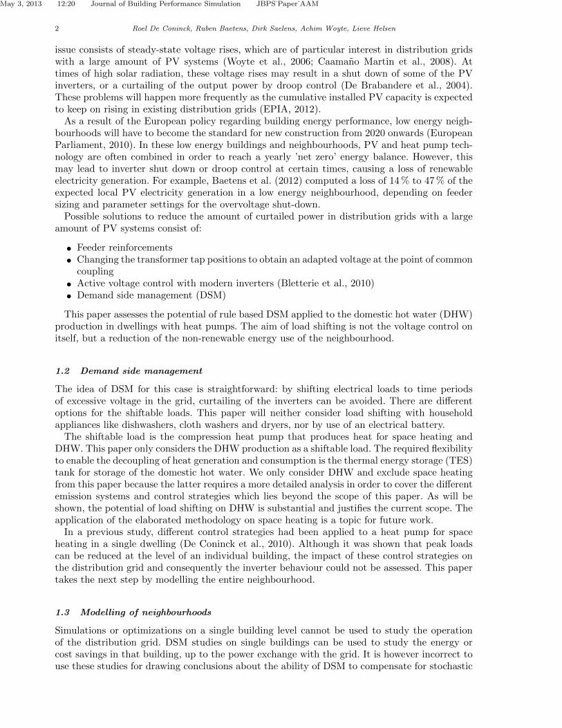
3.4 Aggregated power profiles

In order to get a better understanding of the phasing between average PV production and theelectricity consumption we have aggregated the different power profiles in Figure 12 (upper left).This figure shows the aggregated daily power for user electricity consumption, PV productionand HP operation for dwelling 19 which has about 17 % of curtailing losses. The aggregation isdone for the whole year, including days without curtailing.

As Figure 12 (upper left) shows, in dwelling 19, the electricity consumption of appliances andlighting has a morning and evening peak. The heat pump also operates most in the morning



and evening, with a time shift of about two hours (later) compared to the user electricity con-sumption. This can be explained by the morning and evening peaks in water consumption andthe presence of a DHW storage tank causing the HP to reheat the tank after most DHW with-drawals. As a result, the electricity consumption is not well in line with the electricity generationprofile of the PV system. Curtailing typically takes place between 10h-16h.

4. Demand side management

4.1 Rule-based control strategies

The challenge tackled in this paper is to adapt the control of the DHW production in orderto reduce the net yearly electricity consumption of the neighbourhood ENBH. Given the ohmicgrid losses, ENBH will never become zero without increasing the PV capacity compared to thereference case, even though most control strategies can reduce the ohmic losses to a small extent.

As mentioned before, reducing curtailing losses is straightforward: if the local consumptionis increased sufficiently at periods of high grid voltage, the PV inverters will not shut down.This could however increase ENBH instead of decreasing it. Therefore, the aim is not to reducecurtailing losses but ENBH.

The control strategies are divided in three different categories based on the trigger used toinitiate the load shifting. These triggers can be a clock, the power exchange with the grid orthe voltage. When the trigger is activated, the temperature set point in the DHW storage tankTSetDHW is increased. The amount of the temperature increase is a parameter of the control andwill be varied in the analysis. Some additional variants have been defined as shown in Table 3.Only rule-based control strategies are considered in this paper. Comparing rule-based DSM withfull neighbourhood optimal control could be the topic of future research.

For reference: the simulations were executed on desktop computers with two different cpu’s(Intel Xeon(R) at 2.53 GHz and at 3.07 GHz) and depending on the cpu and (primarily) thecontrol strategy the simulation time was between 1.2 and 4.3 days for simulating one year.

4.2 Load shifting

0 2 4 6 8 10 12 14 16 18 20 22 240

500

1000

1500

2000

Agg

rega

ted

pow

er[W

] Reference

0 2 4 6 8 10 12 14 16 18 20 22 240

500

1000

1500

2000ClockDHW,12K

0 2 4 6 8 10 12 14 16 18 20 22 240

500

1000

1500

2000PGrid12K

0 2 4 6 8 10 12 14 16 18 20 22 24Hour of the day

0

500

1000

1500

2000

Agg

rega

ted

pow

er[W

]

VGridfix,12K

Theoretical PV production Consumption users Consumption HP Resulting PV production

0 2 4 6 8 10 12 14 16 18 20 22 24Hour of the day

0

500

1000

1500

2000VGridvar,12K

0 2 4 6 8 10 12 14 16 18 20 22 24Hour of the day

0

500

1000

1500

2000Central12K

Figure 12. Aggregated power density profiles for dwelling 19 with a DHW storage tank of 0.3 m3.



Table 3. Overview of DSM control strategies

Name Trigger for DSM Details Implementation effort

ClockDHW Clock Between 12h00 and 16h00, TSetDHW

is increased.Very low, no sensors required.

PGrid Power exchange of thedwelling with the grid

When the power injection in the gridsurpasses Plim , TSetDHW is increased.Plim is the same regardless PV sizing.

Moderate. Requires powermeasurement, preferentiallybased on inverter output be-fore curtailing and without HPconsumption to avoid unstablecontrol or the need for largehysteresis.

VGridfix Voltage at dwelling’sgrid connection

When the voltage surpasses Vlim ,TSetDHW is increased. Vlim is thesame for all dwellings and is typicallya few Volt lower than 253 V a.

Low, only requires a singlevoltage measurement.

VGridvar Voltage at dwelling’sgrid connection

When the voltage surpasses Vlim ,TSetDHW is increased. Vlim dependson the position of the dwelling in thegrid.

Low on building side, only re-quires a single voltage mea-surement. Power flow calcu-lation required once in orderto determine Vlim for eachdwelling.

Central Voltage at dwelling’sgrid connection andtemperature of DHWtank.

A central intelligence is present withaccess to the voltage and temperatureof the DHW tank in each dwelling.When somewhere in the grid Vlim

is exceeded, TSetDHW of the DHWtank with lowest temperature is in-creased, regardless of the position ofthat dwelling in the grid.

High. Requires centralisedmonitoring and control andcan conflict with privacy ofthe occupants.

a In all simulations with VGridfix , Vlim has been set to 251 V, 2 V lower than the shut-down limit to create a safetymargin.

b The power flow calculation imposes an equal load to all dwellings for which the maximum voltage in the gridreaches 251 V. The corresponding voltage at each connection point is Vlim .

A first strategy for shifting the HP operation is a clock-based increase of TSetDHW . To keepthis DSM control very simple, the temperature is increased at the same time (12h-16h) in everyhouse on all days of the year, even when there is no curtailing risk at that moment or positionin the grid. The aggregated power profiles for ClockDHW ,12K , with a daily temperature increaseof 12 K is shown in Figure 12 (upper middle). We can see a clear shift in the operation of theheat pump with a very sharp peak at 12h. As a consequence, the morning and evening peaks arelargely flattened. The result is a strong reduction of inverter shut-down between 12h and 14h.The effect does not last till 16h as the heat pumps in the neighbourhood switch off one by onewhen the temperature in their respective storage tank reaches the increased TSetDHW .

The voltage increase in the grid is caused by simultaneous injection of surplus electricity by alldwellings. When we try to increase the self-consumption γS at times of high injection power weexpect the curtailing losses to decrease. Figure 12 (upper right) shows the effect of PGrid12K . Theshift of HP operation is much less pronounced as for ClockDHW ,12K . This is because this DSMcontrol is only active on sunny days and the aggregated profile is computed based on all days ofthe year. Nevertheless, the impact on curtailing losses is high, specifically in the morning. In theafternoon, when the storage tanks in the neighbourhood start reaching the increased TSetDHW ,the effect is lower. It has to be noted that in this control strategy, all dwellings participate, evenif they do not suffer from inverter shut-down. As the trigger for DSM is a fixed and identicalPlim for all dwellings, this control will be activated more often for large PV systems.

The reason for inverter shut-down being excessive voltage, it seems more logic to base theDSM strategy on a measurement of the voltage at the dwelling’s grid connection. There aretwo options for setting the voltage limit Vlim at which TSetDHW is increased. In the VGridfix

strategy, Plim is the same for all dwellings (251 V). In VGridvar , Plim depends on the positionof the dwelling and the characteristics of the feeder. The idea is to activate the control in the



dwellings when based on their own voltage measurement there is a good reason to suspect thatcurtailing is about to happen somewhere else. The effect on the aggregated power for bothcontrols with a ∆TSetDHW of 12 K is shown in Figure 12 (lower left and middle). The impact ofsharing the burden among all dwellings can clearly be seen: VGridvar ,12K reduces the curtailinglosses more than VGridfix ,12K .

A more advanced DSM control based on Vlim requires a central management system that hasaccess to all voltages in the grid and the temperatures in the DHW tanks and that can increaseTSetDHW . This way, the controller can select which HP is to start to avoid curtailing. Ideally,the controller would take into account the grid topology and select the dwelling(s) that willhave most effect on the anticipated problem. However, the Central control investigated in thispaper only selects based on storage tank temperature. With a maximum ∆TSetDHW of 12 K, theresulting aggregated power is shown in Figure 12 (lower right). The Central strategy is clearlymore complicated and expensive than all other studied controls as it requires a central systemfor monitoring and control. However, it is still much easier (and cheaper) than model predictivecontrol (MPC) as it does not require weather and user behaviour forecasts, system models andan optimisation framework.

4.3 Resulting net yearly electricity consumption

So far, we have only discussed the load shifting behaviour of the DSM control strategies andthe resulting reduction in curtailing for a single case (dwelling 19). In this section we alsoconsider the effects of the higher average storage tank temperature and shifted heat pumpoperation on the total net electricity consumption of the neighbourhood, ENBH. We define thenet electricity savings as ∆ENBH = ENBH, DSM−ENBH, ref. Figure 13 shows the loss-benefit spacefor the neighbourhood. In this graph, every marker is the final result of a control strategy onneighbourhood level. The number in the marker is the increase in TSetDHW when the controlis activated. The horizontal axis represents the relative electricity demand compared to thereference case. The vertical axis shows the relative curtailing and ohmic losses compared to thereference. Therefore, the reference lies in the origin, and a case for which gains and savings areequal would lie on the status quo line, the diagonal through the origin. The resulting net savingsfor every case ∆ENBH, is the difference between relative savings and relative consumption andis represented by the vertical distance of the marker to the status quo line.

A first remarkable result is the good performance of the most simple control strategy,ClockDHW ,4K . It is the only control for which the electricity demand is substantially lower thanthe reference case −3.4 MWh, and at the same time it is able to reduce curtailing losses by2.3 MWh. These effects add together and result in ∆ENBH of 5.6 MWh. As a matter of fact, nosingle other control strategy can do better. Variants of ClockDHWK with ∆TSetDHW equal to 8 Kor 12 K are much less interesting. They can reduce the curtailing losses a little bit further, butthe savings on electricity demand completely vanish. The reason why ClockDHW ,4K outperformsall other strategies is the fact that besides reducing curtailing losses on sunny days, it also hasa benefit during almost all other days. As pointed out earlier by De Coninck et al. (2010), thetimed increase of TSetDHW shifts the operation of the air-to-water HP to the afternoon, whenthe ambient temperature is often a few degrees higher than in the morning or evening. As longas ∆TSetDHW is low, this effect outweighs the performance loss due to the increased condensertemperature and the additional thermal losses in the TES tank and hydronic circuit. This isconfirmed by the median of the HP’s SPF for all dwellings: it rises from 3.06 in the referencecase to 3.17 for ClockDHW ,4K .

Furthermore, when the tank temperature is temporarily increased, the top of the tank willstill be warm enough after the next DHW withdrawal and the tank does not have to be reheatedas soon as in the reference case. This will improve the stratification in the tank and lead to thefollowing benefits:

• less heat pump cycles, resulting in lower thermal losses of the heat pump and hydronic



-2.0% -1.0% 0.0% 1.0% 2.0% 3.0% 4.0% 5.0% 6.0%Relative increase in electricity demand

0.0%

1.0%

2.0%

3.0%

4.0%

5.0%

6.0%

7.0%

Rel

ativ

ere

duct

ion

incu

rtai

ling

and

ohm

iclo

sses

Status

quo lin

e

∆E NBH=

1.0%

∆E NBH=

2.0%

∆E NBH=

3.0%

Reference curtailing loss

Reference curtailing + ohmic loss

0

12

48

12

8

12

16

8

4

16

4

128

12

18

ClockDHW , vol=0.3 m3

PGrid, vol=0.3 m3

VGridvar, vol=0.3 m3

VGridfix, vol=0.3 m3

Central, vol=0.3 m3

Figure 13. Loss-benefit space for rule-based DSM with 0.3 m3 DHW storage tank.

circuit

• lower condenser temperatures at the start of the next tank heating cycle, resulting in ahigher SPF

• lower average temperatures at the bottom and middle of the tank, resulting in lower thermallosses for these layers.

The cumulative result of these effects is a reduction of total thermal losses for the entire neigh-bourhood of 4.2 MWh (= 8.5 %). Of course, the other strategies benefit from similar effects, butonly during the sunny periods when their DSM strategy is activated. This means that all otherstrategies can be combined with ClockDHW ,4K in order to try to combine the benefits from bothstrategies. Some results of combined strategies are discussed in section 4.5.

Figure 13 also shows the results for the other strategies for different values of ∆TSetDHW .We see that for all strategies, both electricity demand and reduction of curtailing losses increase



with rising values of ∆TSetDHW . Therefore, the net neighbourhood savings, ∆ENBH tend toshow a maximum as a function of ∆TSetDHW . Sometimes the maximum does not seem to bereached because simulations with temperature increases of more than 18 K are not performed tostay within the validity range of the heat pump model.

There is a clear rank in the performance of the control strategies. We put them in order ofdecreasing effectiveness (based on ∆ENBH) , and indicate which ∆TSetDHW gives the best result:

(1) ClockDHW , optimal ∆TSetDHW = 4 K(2) Central , optimal ∆TSetDHW = 12 K and 18 K(3) VGridvar , optimal ∆TSetDHW = 12 K(4) PGrid , optimal ∆TSetDHW = 12 K(5) VGridfix , optimal ∆TSetDHW = 16 K.

Overall, we can conclude that for a 0.3 m3 storage tank and with the proper ∆TSetDHW , theserule-based control strategies are able to reduce ENBH by 3.0 MWh to 5.6 MWh. This correspondsto a reduction of curtailing losses by 35 % to 65 %. Compared to the total electricity demand ofthe neighbourhood (without taking into account PV production), these savings represent 1.6 %to 3.0 %.

4.4 Effect of increased storage tank size

All results discussed so far were based on a DHW storage tank of 0.3 m3. It is clear that byincreasing the volume of this tank, the system will be able to reduce the curtailing losses evenmore. However, the thermal losses will also be higher, and may overcompensate the benefits ofadditional load shifting. Figure 14 shows the results with a storage tank size of 0.5 m3. In thisfigure, also the reference case has this larger DHW tank. This does barely influence the referencecurtailing losses, but increases the ENBH of the reference case by 1.6 MWh.

As expected, all strategies are able to reduce the curtailing losses further than with a 0.3 m3

storage tank. The most notable change is a reduced performance of the ClockDHW . Whereasfor all other strategies, the position of the markers is very similar to the previous results, themarkers of ClockDHW are clearly shifted to the right. This specifically means that the increasedsystem performance of ClockDHW ,4K is less pronounced with a larger storage tank. As a result,this strategy is outperformed by the more complicated control strategies VGridvar and Central .

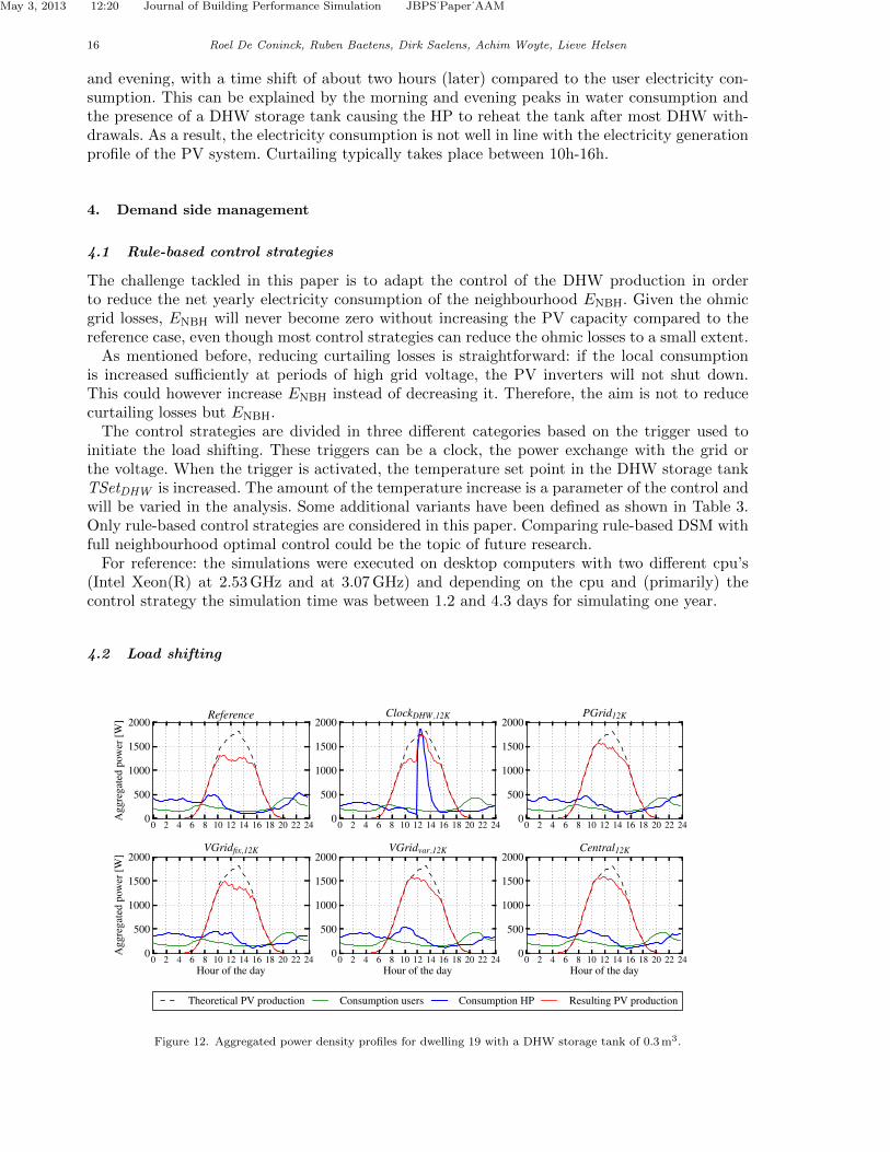
The real merit of a larger storage tank has to be evaluated by comparison with the originalreference case which has the smaller tank. This is done in Figure 15, where the reference casewith DHW tank of 0.3 m3 is placed in the origin. In a first instance, we do not discuss the threemarkers at the end of the arrows (they will be discussed in the next section). From this figure wecan clearly see the shift of all cases with a DHW tank of 0.5 m3 to the right and upwards (exceptfor the reference). However, none of the cases with a larger storage tank is able to compensatethe additional electricity demand by stronger reduction of curtailing losses. This brings us to animportant conclusion of this study: with the simulated control strategies it does not make senseto install additional thermal energy storage to increase the DSM capabilities of the systems.

4.5 Combinations with ClockDHW ,4K

Finally, we want to combine the merits of the most simple strategy on the days without curtailingwith the performance of the advanced strategies on the days with curtailing. This has beensimulated for three cases and visualised with arrows in Figure 15.

The combinations are indeed an improvement of the original strategies. The improvement inenergy efficiency is a little bit smaller than anticipated, but on the other hand there is even anadditional reduction of curtailing losses. However, our previous conclusion holds: the systemswith the smaller storage tank show a better energy performance.

The best results are obtained with the combination of ClockDHW ,4K and VGridvar ,16K . This




0.0%

1.0%

2.0%

3.0%

4.0%

5.0%

6.0%

7.0%

Rel

ativ

ere

duct

ion

incu

rtai

ling

and

ohm

iclo

sses

Status

quo lin

e

∆E NBH=

1.0%

∆E NBH=

2.0%

∆E NBH=

3.0%



0

84

12

8

12

16

4

8

812

16

4

8

1218


PGrid, vol=0.5 m3


VGridfix, vol=0.5 m3

Central, vol=0.5 m3

Figure 14. Loss-benefit space for rule-based DSM with 0.5 m3 DHW storage tank.

simulation realised a ∆ENBH of 6.4 MWh which corresponds to a reduction of curtailing lossesby 74 % or a reduction of ENBH by 3.4 %. We could have simulated more combinations and othervalues for ∆TSetDHW . For instance, from Figure 15 it can be anticipated that a combinationof ClockDHW ,4K with VGridvar ,12K or Central18K will bring ∆ENBH even higher. There areprobably also other control strategies worth investigating. However, with the current results, wealready show that simple rule-based controls are able to strongly reduce curtailing losses in lowenergy dwellings with a high PV penetration while decreasing the net electricity demand.

4.6 Load matching and grid interaction indicators

The aim of this study is to decrease the net electricity consumption of the neighbourhood ENBH

as a whole by avoiding PV inverter shut-down. Therefore, a neighbourhood model has been




0.0%

1.0%

2.0%

3.0%

4.0%

5.0%

6.0%

7.0%

Rel

ativ

ere

duct

ion

incu

rtai

ling

and

ohm

iclo

sses

Status

quo lin

e

ΔENBH=

1.0%

ΔENBH=

2.0%

ΔENBH=

3.0%



0

12

48

12

8

12

16

8

16

4

16

4

128

12

18

Status

quo lin

e

ΔENBH=

1.0%

ΔENBH=

2.0%

ΔENBH=

3.0%



0

84

12

8

12

16

4

8

16

812

16

4

8

1218

18


PGrid, vol=0.3 m3


VGridf x, vol=0.3 m3

Central, vol=0.3 m3


PGrid, vol=0.5 m3


VGridf x, vol=0.5 m3

Central, vol=0.5 m3

Figure 15. Loss-benefit space for rule-based DSM with 300 l and 500 l DHW storage tank. The three markers at the end ofarrows are combinations of that control strategy with ClockDHW ,4K

developed in Modelica. When such a model is not available and the only tool at hand is a stand-alone building simulation program, the interaction of the building with the electricity grid canbe characterized by load matching and grid impact (LMGI) indicators. LMGI indicators aredefined by different authors (Salom et al., 2011; Verbruggen et al., 2011; Baetens et al., 2012)in order to quantify the balance between local electricity generation and consumption and theconsequences of distributed generation on the electricity grid. In this section we will considermore specifically the self-consumption γS and self-generation γD, calculated as

γS =

∫min{PD, PS}dt∫

PSdt(7)



γD =

∫min{PD, PS}dt∫

PDdt(8)

where PS is the local power supply (ie. PV production) and PD the local power demand. Theterm min{PD, PS} represents the part of the power demand instantaneously covered by the localPV power supply or the part of the power supply covered by the demand (Baetens et al., 2012).

These indicators have to be used with caution because they are biased by bad control andinefficiency. For example, the operation of a heat pump at very high temperatures in order tostore thermal energy during times of local overproduction of electricity will clearly increase theself-consumption. However, there is no guaranteed energy saving on total system level and/orreduction in greenhouse gas emissions. The very contrary can be true, as will be shown here.

A scatter plot of the average self-consumption and self-generation for all dwellings in theneighbourhood and for all investigated control strategies is shown in Figure 16. In this figure,both indicators are plotted as a function of the relative energy savings of the neighbourhood∆ENBH. This figure shows how biased these LMGI indicators can be. Although it is true that allefficient strategies have high indicators, the opposite is not true: a high indicator does not implya high energy efficiency. As an example, we can consider the points in the left upper corner of thefigure: these cases have a higher self-consumption and self-generation than the reference case,but result in an increased electricity consumption of the neighbourhood. In order to save energy,it should therefore never be the aim to increase the self-consumption of individual buildings assuch.

−6 −4 −2 0 2 4 6 8∆ENBH [MWh]

0.20

0.25

0.30

0.35

0.40

γ s,γ

d[−

]

Self-consumption, γs

Self-generation, γd

Figure 16. Scatter plot of average self-consumption and self-generation for all control strategies versus ∆ENBH

This reasoning can be extended to neighbourhoods, districts, countries. As long as the studiedsystem is interfaced with other consumers and production units which are not included in themodel, side-effects on the global scale occur and conclusions on global system level have to bedrawn with care. Sometimes such conclusions are simply not valid. It is therefore not the aimto increase the self-consumption of the neighbourhood as a whole.



5. Summary and conclusions

We have presented an integrated bottom-up approach to model and simulate neighbourhoodswith Modelica. The model includes multiple single-family dwellings and the low voltage grid towhich they are connected. For each of the dwellings, the model incorporates a thermal buildingmodel, HVAC system with DHW storage tank, air-to-water heat pump and floor heating, and afully stochastic user behaviour model for presence, appliances, lighting and DHW use.

The model is used to study inverter curtailing losses in a low energy neighbourhood with33 dwellings with a high total installed PV power. In the reference case, inverter shut-downcauses an electricity generation loss of 8.6 MWh or 4.6 % of the initial electricity demand of theneighbourhood. A first conclusion is that these losses are much lower than previously reportedresults under similar circumstances. The reason can be found in changed regulations, allowingvoltage deviations in the distribution grid of up to 10 % instead of 6 % previously.

In order to reduce this loss, different rule-based DSM strategies applied to the DHW productionare proposed and simulated, both for a 0.3 m3 and 0.5 m3 DHW tank. Different conclusions aredrawn from the results.

• The curtailing losses can be reduced to a large extent by different rule-based control strate-gies. However, the net energy saving is generally smaller than the reduction in curtailinglosses because of increased thermal losses.

• The simulated controls realise net savings of up to 74 % of the original curtailing losses. Thiscorresponds to a reduction of the electricity demand of the total neighbourhood (withouttaking PV generation into account) by 3.4 %.

• Rule-based control strategies can be very straightforward. The most simple one,ClockDHW ,4K , is just a timed increase of the set temperature in the storage tank andis difficult to beat. The most advanced control under investigation, Central brings onlylimited additional energy savings compared to VGridvar .

• The best results are obtained when the whole neighbourhood participates in the load shift-ing, including dwellings that never experience curtailing. This can be accomplished whenthe trigger for DSM is a (fixed) injection power or a dwelling-dependent voltage limit (whichleads to better results).

• Load matching and grid interaction indicators must be used with care. Both the very effec-tive and ineffective control strategies can have a high self-consumption γs and self-generationγd. This result can be generalized: it is often not possible to draw valid conclusions on aglobal scale from a model of a local system.

• Increasing the DHW storage size from 0.3 m3 to 0.5 m3 always results in a higher electricityconsumption, regardless of the control strategy used.

This study shows that even with small TES tanks and very simple controls, PV inverter shut-down can strongly be reduced. Model predictive control strategies are expected to lead to betterresults. However, they require significantly higher investments which may not be compensatedby additional savings. Future research has to concentrate on the window of improvement byMPC over the already successful rule-based controls.

6. Acknowledgement

The authors gratefully acknowledge the KU Leuven Energy Institute (EI) for funding this re-search through granting the project entitled Optimized energy networks for buildings and theEuropean Commission for granting the Performance Plus project in the 7th Framework Pro-gramme.


REFERENCES 25

References

Ackermann, T. and V. Knyazkin (2002). Interaction between distributed generation and thedistribution network: operation aspects. In IEEE/PES Transmission and Distribution Con-ference and Exhibition, Volume 2, pp. 1357–1362.

Baetens, R., R. De Coninck, J. Van Roy, B. Verbruggen, J. Driesen, L. Helsen, and D. Saelens(2012). Assessing electrical bottlenecks at feeder level for residential net zero-energy build-ings by integrated system simulation. Applied Energy 96 (Special issue on Smart Grids,Renewable Energy Integration, and Climate Change Mitigation - Future Electric EnergySystems), 74–83.

Becker, B. and K. Stogsdill (1990). Development of Hot Water Use Data Base. In ASHRAETransactions, Volume 96, Atlanta, GA, pp. 422–427. American Society of Heating, Refrig-erating and Air Conditioning Engineers.

Bletterie, B., A. Gorsek, B. Uljanic, A. Woyte, T. Vu Van, F. Truyens, and J. Jahn (2010).Enhancement of the Network Hosting CapacityClearing Space for/with PV. In EuropeanPhotovoltaic Solar Energy Conference.

Caamano Martin, E., H. Laukamp, M. Jantsch, T. Erge, J. Thornycroft, H. De Moor, S. Cobben,D. Suna, and B. Gaiddon (2008). Interaction Between Photovoltaic Distributed Generationand Electricity Networks. Progress in photovoltaics: research and applications 16 (7), 629–643.

Cheng, V. and K. Steemers (2011). Modelling domestic energy consumption at district scale: Atool to support national and local energy policies. Environmental Modelling & Software 26,1186–1198.

Daikin Europe N.V. (2006). Technical data Altherma ERYQ007A, EKHB007A / EKHBX007A,EKSWW150-300. Oostende.

De Brabandere, K., A. Woyte, R. Belmans, and J. Nijs (2004). Prevention of inverter voltagetripping in high density PV grids. In 19th EU-PVSEC, Paris, Number June, pp. 4–7.

De Coninck, R., R. Baetens, B. Verbruggen, J. Driesen, D. Saelens, and L. Helsen (2010). Mod-elling and simulation of a grid connected photovoltaic heat pump system with thermalenergy storage using Modelica. In P. Andre, S. Bertagnolio, and V. Lemort (Eds.), 8th In-ternational Conference on System Simulation in Buildings (SSB2010), Number June, Liege,pp. P177.

De Soto, W., S. A. Klein, and W. A. Beckman (2006, January). Improvement and validation ofa model for photovoltaic array performance. Solar Energy 80 (1), 78–88.

Dugan, R. and T. McDermott (2001). Operating conflicts for distributed generation on distri-bution systems. In Proceedings of the 45th Rural Electric Power Conference, Little Rock,AR, USA, pp. A3/1–A3/6. IEEE.

EPIA (2012). Global market outlook for photovoltaics until 2016. (EPIA).European Parliament (2010). Directive 2010/31/EU on the energy performance of buildings

(recast). pp. 13–35.Fairey, P. and D. Parker (2004). A Review of Hot Water Draw Profiles Used in Performance

Analysis of Residential Domestic Hot Water Systems. Florida Solar Energy Center.FOD Economie (2008). Bevolking - Private, grootte en collectieve huishoudens. Technical Report

http://tinyurl.com/y8o662r (accessed on 22 January 2013).Haller, M. Y., C. a. Cruickshank, W. Streicher, S. J. Harrison, E. Andersen, and S. Furbo (2009,

October). Methods to determine stratification efficiency of thermal energy storage processesReview and theoretical comparison. Solar Energy 83 (10), 1847–1860.

Han, Y., R. Wang, and Y. Dai (2009, June). Thermal stratification within the water tank.Renewable and Sustainable Energy Reviews 13 (5), 1014–1026.

Hastings, S. (2004, April). Breaking the heating barrier. Energy and Buildings 36 (4), 373–380.Hendron, R. and J. Burch (2007). Development of standardized domestic hot water event sched-

ules for residential buildings. In Energy Sustainability 2007, Number August.


26 REFERENCES

Jordan, U. and K. Vajen (2001). Realistic Domestic Hot-Water Profiles in Different Time Scales.Marburg.

Kersting, W. (2001). Radial distribution test feeders. IEEE Power Engineering Society WinterMeeting, 2001 (C), 908–912.

Kleinbach, E., W. Beckman, and S. Klein (1993, February). Performance study of one-dimensional models for stratified thermal storage tanks. Solar Energy 50 (2), 155–166.

Lechner, H. (1998). Analysis of Energy Efficiency of Domestic Electric Storage Water Heaters.Study for the Directorate General for Energy (DGXVII) of the Commission of the EuropeanCommunities Contract No. SAVE-4.1031/E/95-013.

Loga, T., N. Diefenbach, C. Balaras, E. Dascalaki, M. S. Zavrl, A. Rakuscek, V. Corrado,S. Corgnati, H. Despretz, C. Roarty, M. Hanratty, B. Sheldrik, W. Cyx, M. Popiolek,J. Kwiatowski, M. GroB, C. Spitzbart, Z. Georgiev, S. Lakimova, T. Vimmr, K. B. Wittchen,and J. Kragh (2009). Use of building typologies for energy performance assessment of na-tional building stocks. Existent experiences in European countries and common approach.Technical Report June 2009, First TABULA Synthesis report.

Manfren, M., P. Caputo, and G. Costa (2011). Paradigm shift in urban energy systems throughdistributed generation : Methods and models. Applied Energy 88 (4), 1032–1048.

Marsh, R. (1996). Sustainable housing design : an integrated approach. Ph. D. thesis, Universityof Cambridge.

Mather, D., K. Hollands, and J. Wright (2002, July). Single- and multi-tank energy storage forsolar heating systems: fundamentals. Solar Energy 73 (1), 3–13.

Newton, B. (1995). Modeling of Solar Storage Tanks. Ph. D. thesis, University of Wisconsin-Madison.

Olesen, B. (2001). Control of floor heating and cooling systems. In CLIMA-2000, NumberSeptember, pp. 15–18.

Richardson, I., M. Thomson, D. Infield, and C. Clifford (2010, October). Domestic electricityuse: A high-resolution energy demand model. Energy and Buildings 42 (10), 1878–1887.

Richardson, I., M. Thomson, D. Infield, and A. Delahunty (2009). Domestic lighting: A high-resolution energy demand model. Energy and Buildings 41 (7), 781–789.

Rosen, M. a., R. Tang, and I. Dincer (2004, February). Effect of stratification on energy and ex-ergy capacities in thermal storage systems. International Journal of Energy Research 28 (2),177–193.

Salom, J., J. Widen, J. Candanedo, I. Sartori, K. Voss, and A. J. Marszal (2011). UnderstandingNet Zero Energy Buildings: Evaluation of load matching and grid interaction indicators. InProceedings of Building Simulation 2011, Volume 6, Sydney, Australia, pp. 2514–2521.

Sanyo (2008). HIP-230HDE1 photovoltaic module. http://www.technosun.com/eu/downloads/search-documentation.php (accessed on 22 January 2013).

Sera, D., R. Teodorescu, and P. Rodriguez (2007). PV panel model based on datasheet values.IEEE (4), 2392–2396.

Stokes, M., M. Rylatt, and K. Lomas (2004). A simple model of domestic lighting demand.Energy and Buildings 36 (2), 103–116.

SynerGrid (2012). Specifieke technische voorschriften voor decentrale productie-installaties diein parallel werken met het distributienet. (C10/11 - revisie 4 juni 2012).

Verbruggen, B., R. De Coninck, R. Baetens, D. Saelens, L. Helsen, and J. Driesen (2011). Gridimpact indicators for active building simulation. In Innovative Smart Grid Technologies(ISGT), 2011 IEEE PES, Number 2, pp. 1–6. IEEE.

Viessmann (2011). Vitocell- 100-V, 390 liter, Datenblatt. http://tinyurl.com/cdpv8rr (accessedon 21 April 2013).

Wetter, M. (2009). Modelica Library for Building Heating, Ventilation and Air-ConditioningSystems. In The 7th International Modelica Conference, pp. 393–402. The Modelica Asso-ciation.

Widen, J., M. Lundh, I. Vassileva, E. Dahlquist, K. Ellega rd, and E. Wackelga rd (2009,


REFERENCES 27

July). Constructing load profiles for household electricity and hot water from time-usedataModelling approach and validation. Energy and Buildings 41 (7), 753–768.

Woyte, A., V. V. Thong, R. Belmans, and J. Nijs (2006). Voltage fluctuations on distributionlevel introduced by photovoltaic systems. IEEE Transactions on Energy Conversion 21 (1),202–209.

Zurigat, Y. H., K. J. Maloney, and A. J. Ghajar (1989). A comparison study of one-dimensional models for stratified thermal storage tanks. Journal of Solar Energy Engi-neering;(USA) 111 (3).

article rule-based demand side management of domestic … · this saturation is often ......

Documents