article on dsp
TRANSCRIPT

DESIGN AND IMPLEMENTATION OF A DSP BASED ACTIVE NOISE CONTROLER FOR HEADSETS
A THESIS SUBMITTED TO THE GRADUATE SCHOOL OF NATURAL AND APPLIED SCIENCES
OF THE MIDDLE EAST TECHNICAL UNIVERSITY
BY
AHMET TOKATLI
IN PARTIAL FULLFILLMENT OF THE REQUIREMENTS FOR
DEGREE OF THE MASTER OF SCIENCE IN
ELECTRICAL AND ELECTRONICS ENGINEERING
AUGUST 2004

Approval of the Graduate School of Natural and Applied Sciences
__________________________
Prof. Dr. Canan Özgen
Director
I certify that this thesis satisfies all the requirements as a thesis for the degree of
Master of Science
__________________________
Prof. Dr. Mübeccel Demirekler
Head of Department
This is to certify that we have read this thesis and that in our opinion it is fully
adequate, in scope and quality, as a thesis for the degree of Master of Science.
__________________________
Assoc. Prof. Dr. Tolga Çiloğlu
Supervisor
Examining Committee Members
Prof. Dr. Buyurman Baykal (METU EE) _________________________
Assoc. Prof. Dr. Tolga Çiloğlu (METU EE) __________________________
Assoc. Prof. Dr. Engin Tuncer (METU EE) __________________________
Assist. Prof. Dr. Çağatay Candan (METU EE) __________________________
Assist. Prof. Dr. Yakup Özkazanç (HU EE) __________________________

iii
I hereby declare that all information in this document has been obtained and
presented in accordance with academic rules and ethical conduct. I also
declare that, as required by these rules and conduct, I have fully cited and
referenced all material and results that are not original to this work.
Name, Last name :
Signature :

iv
ABSTRACT
DESIGN AND IMPLEMENTATION OF A DSP BASED ACTIVE NOISE CONTROLER FOR HEADSETS
Tokatlı, Ahmet
M.S., The Department of Electrical and Electronics Engineering Supervisor: Assoc. Prof. Dr. Tolga Çiloğlu
August 2004, 84 pages
The design of a battery-powered, portable headphone active noise control
system with TI TMS320C5416 DSP is described. The preliminary implementation
of the system on a C5416 DSK is also explained. The problems of fixed-point
implementation are described and solutions are proposed. Sign-sign Fx-LMS
algorithm with a dead-zone is introduced and used as the adaptation algorithm.
Effective use of dynamic range to improve the accuracy in filtering operations is
discussed. Details of the designed battery-powered DSP board are given and board
software development process is explained. The DSK system and designed
portable system is compared against two commercially available analog systems
under three different types of noises; composition of tones, drill noise and
propeller plane cabin noise. The results reveal that adaptive system has better
overall performance.

v
Keywords: Feedforward and feedback active noise control, headphone ANC, FX-
LMS, Sign–Sign FX-LMS

vi
ÖZ
KULAKLIKLAR İÇİN DSP TABANLI BİR AKTİF GÜRÜLTÜ KONTROL SİSTEMİ
Tokatlı, Ahmet Yüksek Lisans, Elektrik ve Elektronik Mühendisliği Bölümü
Tez Yöneticisi: Doç. Dr. Tolga Çiloğlu Ağustos 2004, 84 sayfa
Pille çalışabilen taşınabilir aktif gürültü kontrollü kulaklık sisteminin TI
TMS320C5416 DSP ile tasarımı anlatılmıştır. Aktif gürültü kontrollü kulaklık
sisteminin C5416 DSK kartı ile gerçekleştirimi açıklanmıştır. Sabit–nokta
gerçektirimi problemleri anlatılmış ve çözümler sunulmuştur. Ölü bölgeli Sign-
sign Fx-LMS algoritması uyarlama algoritması olarak açıklanmıştır. Süzgeçleme
operasyonunda kesinliği arttıram için dinamik alanın verimli kullanımı
tartışılmıştır. Tasarlanan pille çalışan SSİ kartı detaylandırılmış ve kart yazılım
geliştirme süreci açıklanmıştır. DSK sistemi ve tasarlanan taşınabilir sistem iki
ticari olarak satılan analog sistemle üç farklı gürültü tipinde karşılaştırılmıştır;
tonların birleşimi, matkap gürültüsü, pervaneli uçak kabin gürültüsü. Sonuçlar
uyalamalı sistem daha iyi toplam performansa sahip olduğunu ortaya çıkarmıştır.
Anahtar Kelimeler: İleri besleme ve geri besleme aktif gürültü azaltımı,
kulaklıklı AGK, FX-LMS, Sign–Sign FX-LMS

vii
ACKNOWLEDGEMENTS
I would like to thank my supervisor, Tolga Çiloğlu, for providing me the
opportunity to pursue and finish this degree; his guidance and encouragements
helped me a lot in completing this study. He has been a good igniter when I fell off
in performance.
I would like to thank DPT, TÜBİTAK for their financial support to the my
study and also TI for their free tool supports.
I would also like to thank my friends, Turgay Koç, Dinç ACAR, Özkan
Ünver for their moral support.

viii
TABLE OF CONTENTS
ABSTRACT............................................................................................................. IV
ÖZ ............................................................................................................................VI
ACKNOWLEDGEMENTS ....................................................................................VII
TABLE OF CONTENTS...................................................................................... VIII
LIST OF FIGURES.................................................................................................XII
LIST OF TABLES ................................................................................................. XV
LIST OF ABBREVIATIONS............................................................................... XVI
1. INTRODUCTION.......................................................................................... 1
1.1 Scope of the Thesis ................................................................................ 4
2. THEORETICAL BACKGROUND............................................................... 6
2.1 Wiener Filtering ..................................................................................... 6
2.2 Adaptive Filtering Algorithms ............................................................... 8
2.2.1 Least Mean Square Method ........................................................... 9
2.2.2 Normalized LMS Algorithm........................................................ 10
2.2.3 Sign LMS and Sign–Data LMS algorithms ................................. 11

ix
2.2.4 Sign–Sign LMS algorithm ........................................................... 12
3. ADAPTIVE ANC SYSTEMS ..................................................................... 13
3.1 Introduction .......................................................................................... 13
3.2 ANC system configurations ................................................................. 13
3.3 The Concept of Secondary Path in ANC Systems ............................... 15
3.4 Fx-LMS Algorithm .............................................................................. 17
3.4.1 Derivation of Fx-LMS algorithm................................................. 18
3.5 Sign–sign Fx-LMS Algorithm ............................................................. 21
3.6 Single Channel Feedback ANC ........................................................... 21
3.7 Offline Secondary Path Modelling....................................................... 23
4. IMPLEMENTATION ISSUES.................................................................... 24
4.1 Introduction .......................................................................................... 24
4.2 Dead-zone Mechanism......................................................................... 24
4.2.1 Some Theoretical Results for the Use of Dead-zone ................... 29
4.3 Efficient Use of Dynamic Range in the Fixed-Point Implementation . 32
5. DSK IMPLEMENTATION......................................................................... 34
5.1 Introduction .......................................................................................... 34
5.2 Numerical Evaluations in Fixed Point Arithmetic ............................... 34
5.3 Hardware setup..................................................................................... 35
5.4 Software implementations.................................................................... 36
5.4.1 Secondary Path Modeling ............................................................ 36
5.4.2 Noise Cancellation ....................................................................... 39
6. PORTABLE DSP BOARD DESIGN .......................................................... 43
6.1 Introduction .......................................................................................... 43

x
6.2 Design and Production Procedure........................................................ 43
6.3 Detailed Board Features....................................................................... 45
6.3.1 DSP Chip...................................................................................... 46
6.3.2 A/D–D/A Conversion................................................................... 46
6.3.3 Boot Memory ............................................................................... 48
6.3.4 Power Management...................................................................... 48
6.3.5 Emulation Interface...................................................................... 48
6.3.6 Analog Inputs and Outputs........................................................... 49
6.3.7 Power Consumption and Cost ...................................................... 49
6.4 Debugging and Emulation.................................................................... 51
6.5 Software ............................................................................................... 52
7. EXPERIMENTAL RESULTS AND DISCUSSION................................... 53
7.1 Introduction .......................................................................................... 53
7.2 DSK Implementation Experiments ...................................................... 54
7.2.1 Tonal Noise Performance Test..................................................... 54
7.2.2 Drill Noise Performance Test....................................................... 56
7.2.3 Propeller Plane Cabin Noise Performance Test ........................... 57
7.3 Portable System Experiments .............................................................. 58
7.3.1 Tonal Noise Performance Test..................................................... 58
7.3.2 Drill Noise Performance Test....................................................... 59
7.3.3 Propeller Plane Cabin Noise Performance Test ........................... 59
7.4 Analog System Experiments ................................................................ 60
7.4.1 Tonal Noise Performance Tests ................................................... 61
7.4.2 Drill Noise Performance Tests ..................................................... 62

xi
7.4.3 Propeller Plane Cabin Noise Performance Tests ......................... 64
7.5 Discussion of the Tests......................................................................... 65
7.6 Fixed-point Fx-LMS versus Fixed-point Sign-Sign Fx-LMS.............. 69
7.6.1 Fixed-point Fx-LMS algorithm.................................................... 69
7.6.2 Fixed-point Fx-LMS versus Fixed-point Sign-Sign Fx-LMS...... 72
7.6.3 Effect of Dead-Zone to the Sign-Sign Fx-LMS Algorithm ......... 73
7.7 Floating-point Fx-LMS vs Floating-point Sign-Sign Fx-LMS............ 76
8. CONCLUSION............................................................................................ 78
8.1 Future Work ......................................................................................... 80
REFERENCES......................................................................................................... 81

xii
LIST OF FIGURES
Figure 1.1: Illustration of superposition principle...................................................... 2
Figure 2.1 Discrete time system................................................................................. 7
Figure 3.1: Adaptive feedforward ANC system. ..................................................... 14
Figure 3.2: System identification block diagram. .................................................... 14
Figure 3.3: Adaptive feedback ANC system............................................................ 15
Figure 3.4: Feedback system.................................................................................... 16
Figure 3.5: Adaptive Feedback ANC system........................................................... 17
Figure 3.6: Classical active noise control with identical filter................................. 18
Figure 3.7: Feedback ANC system. .......................................................................... 20
Figure 3.8: Redrawn Feedback ANC system with reference signal sysnthesis and
adaptation. ........................................................................................................ 22
Figure 3.9: Secondary path modeling block diagram. ............................................. 23
Figure 4.1 No dead-zone and no noise. a) Comparison of error spectra before and
after adaptation. b) Coefficient values after adaptation. .................................. 25
Figure 4.2 Large dead-zone and no noise. a) Comparison of error spectra before and
after adaptation. b) Coefficient values after adaptation. .................................. 27
Figure 4.3 Large dead-zone with noise. a) Comparison of error spectra before and
after adaptation. b) Coefficient values after adaptation. .................................. 27

xiii
Figure 4.4 Moderate dead-zone size and no noise. a) Comparison of error spectra
before and after adaptation. b) Coefficient values after adaptation ................. 28
Figure 4.5 Moderate dead-zone size with noise. a) Comparison of error spectra
before and after adaptation. b) Coefficient values after adaptation. ................ 29
Figure 5.1 Structure of accumulator A..................................................................... 35
Figure 5.2: 1 sample delay places ............................................................................ 40
Figure 6.1 Block Diagram of DSP Board ................................................................ 45
Figure 6.2 Designed DSP Board .............................................................................. 47
Figure 6.3 XDS510 PP EMULATOR...................................................................... 51
Figure 7.1: Impulse response and magnitude of the frequency response of the
secondary path model....................................................................................... 55
Figure 7.2: Performance test of DSK system with tones. ........................................ 55
Figure 7.3: Performance test of DSK system with drill noise.................................. 56
Figure 7.4: Performance test of DSK system with propeller plane cabin noise. ..... 57
Figure 7.5: Performance test of portable system with tonal noise. .......................... 58
Figure 7.6: Performance test of portable system with drill noise. ........................... 59
Figure 7.7: Performance test of portable system with propeller plane cabin noise . 60
Figure 7.8: Performance test of system-1 headphone with tones............................. 61
Figure 7.9: Performance test of system-2 headphone with tones............................. 62
Figure 7.10: Performance test of system-1 headphone with drill noise. .................. 63
Figure 7.11: Performance test of system-2 headphone with drill noise. .................. 63
Figure 7.12: Performance test of system-1 headphone with propeller plane cabin
noise. ................................................................................................................ 64

xiv
Figure 7.13: Performance test of system-2 headphone with propeller plane cabin
noise. ................................................................................................................ 65
Figure 7.14:Fx-LMS simulation with sine wave amplitude = 20000. ..................... 70
Figure 7.15:Fx-LMS simulation with sine wave amplitude = 5000. ....................... 71
Figure 7.16:Comparison Fx-LMS with Sign-sign Fx-LMS..................................... 72
Figure 7.17:Comparison Fx-LMS with Sign-sign Fx-LMS with dead-zone. .......... 74
Figure 7.18:Comparison Fx-LMS with Sign-sign Fx-LMS with dead-zone. .......... 75
Figure 7.19:Floating-point comparison of Fx-LMS with Sign-sign Fx-LMS. ........ 77

xv
LIST OF TABLES
Table 6-1: Approximate prices of the components and PCB production in US
dollars............................................................................................................... 50
Table 7-1: Attenuation levels of the systems with tonal noise................................. 66
Table 7-2: Attenuation levels of the systems with drill noise.................................. 67
Table 7-3: Attenuation levels of the systems with propeller plane cabin noise....... 68

xvi
LIST OF ABBREVIATIONS
ANC: Active Noise Control
DSP: Digital Signal Processing
PC: Personal Computer
MSE: Mean-Squared Error
Cool-Edit: Sound Editor Program by Synthrillium Software
Corporation
CCS: Texas Instruments Code Composer Studio software
DSK: Developers Starter Kit
TI: Texas Instruments Company
LMS: Least Mean Square

1
CHAPTER 1
1. INTRODUCTION
INTRODUCTION
Acoustic noise has been a serious problem by the widespread use of
industrial equipments such as engines, fans and compressors. Traditional
approaches to acoustic noise cancellation use passive techniques like enclosures,
barriers and silencers to attenuate noise [1]- [2]. These passive silencers have high
attenuation over a broad frequency range, but they are large, costly and ineffective
at low frequencies because the attenuation of a passive silencer decreases when
wavelength of noise compared to the silencer dimension increases [3].
Active noise control (ANC) has been introduced [4] as a complementary
action against the deficiencies of passive noise reduction techniques. In ANC [5]-
[9] approach, a canceling sound source is used to attenuate primary noise. ANC
uses superposition principle to reduce noise; it produces an anti-noise and sends it
to the environment. Figure 1.1 illustrates how super position principle works. The
amount of attenuation depends on the accuracy of amplitude and phase of the anti-
noise with respect to those of the noise.
Some of the application areas of ANC are duct noise reduction [10]-[11],
interior noise reduction in cars [12]-[13], aircrafts [14] or buildings [15]-[16] and

2
ear protection and headphone systems [17]-[21]. There are also applications for
communication systems like mobile phones [22]. ANC approach is also used in
active vibration control systems and there are several applications on vibration
control [23]-[24].
Figure 1.1: Illustration of superposition principle
An ANC system may be implemented as a single-channel or multi-channel
system [5]-[8],[25]. A single-channel system has one canceling source, one sensor
to pick residual noise and one reference sensor (in feed forward structures) to pick a
signal as noise reference. Single-channel systems are considered for point wise
source of unwanted noise
sound source controlled
by an ANC system
residual noise after cancellation

3
noise cancellation (like headphones) or when noise emission is from a “lumped”
aperture and canceling source can be co-located with the aperture (like air-
conditioning ducts). Multi-channel systems are necessary when noise reduction has
to be achieved in a volume subject to distributed noise sources (like vehicle cabins
[26])
Headphone is one of the most convenient structures to apply ANC.
Headphones with ANC are available as commercial products [27]-[30] and some of
them have quite satisfactory ANC performance in many practical situations like
cockpits, airport ground personnel, etc where noise reduction is definitely relaxing
for the human. Fixed analog controllers have been preferred on these systems for
reasons of stability, low power consumption, small hardware size and lack of
tracking problems. These systems have noise attenuation around 8-12 dB over the
100-350 Hz frequency band. However, we have observed that ANC performance of
some commercial products with relatively high cost are quite insignificant and most
of the noise reduction is provided by the special ear cup design and its tight
mounting to the head.
Our experiments have shown that it is possible to reliably improve the
attenuation by using adaptive controllers. This is especially true when the noise
contains most of its power in a few narrow band components. We have also
observed that it is possible to achieve a wider band of attenuation. Our motivation
in this study was to investigate the feasibility of an adaptive digital controller for
headphones with regard to noise reduction performance against different types of
noises including tracking capabilities, stable operation of the system under practical

4
requirements (such as put on/put off actions), and compactness of the hardware and
power requirements.
1.1 Scope of the Thesis
This study aims to explore fixed-point implementation performance of the
ANC algorithms applied on a headphone system. It also aims to design a portable
digital ANC headphone system and compare the performance of it with the
commercially available analog ANC headphone systems.
The system developed in this study employs a digital adaptive feedback
controller, for each ear cup of a headphone. In the first phase of the study ANC
algorithms were implemented in Matlab1. In the second stage, algorithms were
implemented on a TI C5416 DSK board to see real time performance of the ANC
algorithm with a fixed-point DSP. Various problems have been encountered and
solutions have been studied in this step. After achieving a satisfactory performance
level with DSK, to make a mobile system; a battery powered DSP board has been
designed and produced.
In the thesis, a theoretical background about adaptive filters is given in the
next chapter. Fundamental aspects of single channel adaptive ANC are described in
Chapter 3. In Chapter 4, practical implementation issues are discussed and in
Chapter 5, DSK implementation of the system is explained. Designed DSP board is
1 Matlab is a registered trademark of Mathworks, Inc.

5
introduced in Chapter 6 and experiments on the DSK implementation and DSP
board for comparing digital systems against analog ones are given in Chapter 7.

6
CHAPTER 2
2. THEORETICAL BACKGROUND
THEORETICAL BACKGROUND
In this chapter, adaptive filtering techniques will be introduced. In the first
section, Wiener filtering concept, which is the basis of the adaptive filtering, will be
described. In the second section, several variants of LMS algorithm will be
described.
2.1 Wiener Filtering
For a discrete time system as shown in Figure 2.1 , the output ( )ny can be
expressed as:
( ) ( ) ( )knxnwnyL
kk −= ∑
−
=
1
0 (2.1)
or ( ) ( ) ( )nnwny T x= (2.2)
In the above equation ( )knx − are the input signals and kw are the filter
coefficients, ( )nx and ( )nw are the corresponding column vectors. ( )ne represents
the difference between the desired response ( )nd and the output signal ( )ny , i.e.

7
( ) ( ) ( )nyndne −= (2.3)
Figure 2.1 Discrete time system
A cost function can be defined as the expected value of the square of the
error signal ( )ne as,
( ) ( )[ ] ( )[ ]2EE neneneJ == (2.4)
To find optimum filter coefficients that minimize cost function, gradient of
the cost function with respect to the coefficients is taken and equated to zero.
( ) ( )[ ]nenxJ E2−=∇ (2.5)
( ) ( )[ ] 0E * =nenx (2.6)
where *e denotes the minimum error. Substituting Equations (2.2) and (2.3) into
(2.6) yields
Digital Filter )(zW +
)(nd
)(ne
)(ny
)(nx

8
{ } { })()()()(* ndnxEnxnxEw TT = (2.7)
where *w denotes the optimum weight vector. The above equation can be rewritten
as
pw =*R (2.8)
where R is the autocorrelation matrix of the input signal and p is the cross-
correlation vector of the input signal and the desired response. The Equation (2.8) is
known as Wiener-Hopf Equation. *w is the vector of the optimum filter coefficients
that minimizes expected value of the square of the error signal (MSE).
2.2 Adaptive Filtering Algorithms
For stationary signals, the solution of the Wiener-Hopf Equation gives
optimal filter coefficients but if the signal is non-stationary, optimal filter
coefficients has to be time-varying. Adaptive filtering methods, which solve
Wiener-Hopf Equation iteratively and tracks changes in a non-stationary signal,
have been developed to tackle with the non-stationary case.
Adaptive controller consists of a transversal filter whose tap weights have to
be driven by an adaptation algorithm. Most of the adaptation algorithms stem from
two basic types: LMS and RLS [33]–[39]. The objective function of LMS is
instantaneous squared error whereas that of RLS is average weighted square error.
LMS and its variants have gained remarkable popularity because of low
9
computational requirement and satisfactory performance. On the other hand, RLS
has faster convergence and lower misadjustment (steady state error).
2.2.1 Least Mean Square Method
The Least Mean Squares (LMS) algorithm is widely used because of its low
computational demand and satisfactory performance. LMS algorithm minimizes the
Mean Square Error (MSE) ( )[ ]2E ne . MSE is a quadratic function of the weights of
the filter. LMS algorithm approximates the steepest descent method, which updates
filter coefficients negative gradient direction of the cost function ( )[ ]2E ne as:
( ) ( ) ( )[ ]( )[ ]2E211 nenn ∇−+=+ µww (2.9)
Steepest descent method is very effective optimization algorithm, but it is
not possible to use it in real-time applications because it requires exact knowledge
of the MSE.
In LMS, instantaneous values of MSE are used, so it does not require exact
knowledge of MSE and can be used in real-time applications. LMS method [33],
[37] computes the filter coefficients as follows:
( ) ( ) [ ]Jnn ∇−+=+ µ211 ww (2.10)
( ) ( )[ ]2
21 nen ∇−+= µw (2.11)

10
where J denotes the instantaneous value of cost function and µ21 is an artificial
gain in order to prevent the unstable divergence. The instantaneous gradient of cost
function can be expressed as the product input signal and the error, i.e.
( ) ( ) ( )nxnene 22 −=∇ (2.12)
From Equations (2.11) and (2.12) update formula of the LMS algorithm can
be written as:
( ) ( ) ( ) ( )nenxnwnw µ+=+1 (2.13)
The gain µ has to satisfy the following condition for convergence:
max
20 λµ << (2.14)
where maxλ is the largest eigenvalue of R .
2.2.2 Normalized LMS Algorithm
Stability and convergence rate of the LMS algorithm is determined by the
step size, which has a bound dependent on the input data )(nx . Therefore, these
performance parameters vary with )(nx . To defeat this inconveniency, update
equation of the LMS algorithm can be rewritten as in Equation (2.15). This
modified algorithm is called as Normalized LMS (NLMS) algorithm [33], [37]
because update term is normalized by the power of the input signal.

11
( ) ( )( )
( ) ( )nenxnx
nwnw 21 µ+=+ (2.15)
NLMS algorithm converges faster than the ordinary LMS algorithm and it is
convergent if the following condition on µ is satisfied.
20 << µ (2.16)
2.2.3 Sign LMS and Sign–Data LMS algorithms
Sign algorithms [36] have been introduced to reduce computational
complexity of the LMS algorithm. Update equation of the sign algorithm is as
follows:
( ) ( ) ( ) ( ))(1 nesignnxnwnw µ+=+ (2.17)
As seen in the update equation sign algorithm requires less multiplications
than the LMS algorithm.
For a single coefficient, sign algorithm does not change direction of the
gradient vector but magnitude of the gradient vector changes. Sign algorithm
minimizes absolute error )(ne instead of the mean square error.
Sign-data algorithm takes sign of the data vector instead of the error. Update
equation is
( ) ( ) ( ) ( )nenxsignnwnw )(1 µ+=+ . (2.18)

12
Although they reduce computational complexity, Sign and Sign-data
algorithms decrease the convergence rate of the LMS algorithm.
2.2.4 Sign–Sign LMS algorithm
Another modified LMS algorithm is sign–sign LMS [36], which takes signs
of the both signals in the update term. Update equation of the sign–sign LMS
algorithm is as follows:
( ) ( ) ( ) ( ))()(1 nesignnxsignnwnw µ+=+ (2.19)
From Equation (2.19) it can be seen that by taking the sign of the two
signals, gradient direction does not change for a single coefficient but the
magnitude of the gradient goes to unity and coefficient update is done by adding or
subtracting step size from coefficients. The direction of the gradient vector changes
from real direction and system follows a new and long path to reach optimal point.
Sign–sign LMS algorithm has very low convergence rate compared with the
other LMS algorithms in the floating-point operations, but it has no multiplication
and algorithmic complexity of the system is reduced extremely.

13
CHAPTER 3
3. ADAPTIVE ANC SYSTEMS
ADAPTIVE ANC SYSTEMS
3.1 Introduction
In this chapter, adaptive ANC systems will be introduced. In the first
section, feedforward and feedback ANC system configurations will be defined. In
Section 3.3, secondary path concept will be explained. In Section 3.4, well-known
ANC algorithm, Fx-LMS algorithm, and in Section 3.5 a modified Fx-LMS
algorithm, sign-sign Fx-LMS algorithm, will be introduced. In the remaining
sections, single-channel feedback ANC system and offline secondary path modeling
algorithm will be mentioned.
3.2 ANC system configurations
ANC systems may operate in either feedforward or feedback configuration.
A duct type single channel feedforward ANC system is seen in Figure 3.1. There
are two microphones and one speaker. One of the microphones (reference
microphone) is placed near the noise source to pick the reference noise signal and
other microphone (error microphone) is placed at the cancellation region. Anti-
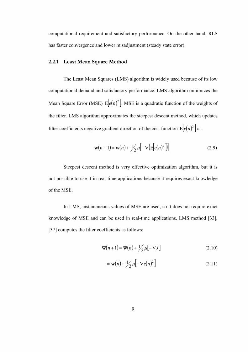
14
noise is created by modifying the reference noise signal and applying it to the
loudspeaker (secondary source). A block diagram of the system is shown in Figure
3.2. The construction in Figure 3.2 is a typical system identification setup. The role
of adaptive controller is to identify the duct transfer function. Controller is adapted
to minimize the power of the residual signal obtained from the error microphone.
Figure 3.1: Adaptive feedforward ANC system.
Figure 3.2: System identification block diagram.
noise
generator
adaptive control
Transfer function of the primary path
Σ
adaptive control
reference mic.
secondary source
noise
source primary path

15
In a feedback ANC system, first proposed by Olson [9], there is no
reference microphone, Figure 3.3. Block diagram of the feedback system is shown
in Figure 3.4, reference signal is estimated in the adaptive control unit; once the
reference signal is obtained, it works similar to a feedforward system.
Feedforward systems are not suitable for headphone applications. The
location or orientation of the headphone may change with the motion of user.
Primary path is affected by this motion and tracking problem is imposed on the
system.
Figure 3.3: Adaptive feedback ANC system.
3.3 The Concept of Secondary Path in ANC Systems
According to the block diagrams of Figure 3.2 and Figure 3.4, the output of the
adaptive controller is directly combined with the noise and resulting error signal is
Adaptive Control
Secondary Source
Error Microphone
Noise Source

16
directly fed back to the controller. This is not the case in practice. There exist a
number of transfer paths on these routes. These include the D/A converter and
amplifier at the output stage of the controller, the loudspeaker, acoustic transfer path
between the loudspeaker and microphone, the microphone, amplifier after the
microphone and finally the A/D converter. The presence of such a path has led the
development of so-called filtered-x type adaptation algorithm[8], [31],[32].
Figure 3.4: Feedback system.
The path described above is called ‘secondary path’. The block diagram in
Figure 3.4 is redrawn in Figure 3.5 where the components A(z) and B(z) of the
secondary path are shown separately.
Filtered-x type adaptation algorithms use a model of secondary path.
Assuming that the secondary path is an LTI system, it is generally modeled by an
FIR filter. The impulse response is identified by an adaptive procedure.
noise generator Σ
adaptive control

17
Identification may be prior to (offline) or during (online) the operation of the noise
cancellation system. In this work, offline method has been used and it will be
described in Section 3.7.
Fx-LMS algorithm has been preferred in this work mainly because of
computational requirements. Fx-LMS algorithm is a modified form of LMS
algorithm that emerged to overcome the problems associated with the presence of
secondary path.
Figure 3.5: Adaptive Feedback ANC system.
3.4 Fx-LMS Algorithm
In ANC applications, since the secondary path transfer function )(zS
follows the adaptive filter, the conventional LMS algorithm has to be modified to
noise
generator Σ
adaptive control
A(z)
B(z)
S(z)

18
ensure convergence. A solution is to place an identical filter of )(zS to the reference
signal path to the weight update of the LMS algorithm. Because the input is filtered,
this algorithm is called filtered–x LMS algorithm.
Figure 3.6: Classical active noise control with identical filter.
3.4.1 Derivation of Fx-LMS algorithm
Figure 3.6 shows an active noise control system scheme with secondary
path and its replica placed at the input of the LMS algorithm. The signals can be
expressed as:
)(')()( nyndne −=
)(*)()()( nynsndne −=
)(ne
)(ny
)(ny′
)(nd
)(nx
)(zW
Primary
Path
)(zS LMS
)(zS
Σ
)(nx
Σ

19
))()((*)()()( nxnwnsndne T−= (3.1)
where,
{ })()( 1 zSZns −=
TL nwnwnwnw ])()......()([)( 110 −=
and,
TLnxnxnxnx ])1()......1()([)( +−−=
The objective of the adaptive filter is to minimize the squared error
( ) ( )nen 2=ξ . To achieve this, LMS algorithm updates the coefficients in the
negative gradient direction with step size µ as:
)(2
)()1( nnwnw ξµ∇−=+ (3.2)
)(])([2)()( 2 nenenen ∇=∇=∇ξ (3.3)
from Equation (3.1)
)(')(*)()( nxnxnsne −=−=∇ (3.4)
where,
TLnxnxnxnx ])1(')......1(')('[)(' +−−=
Therefore, gradient estimate becomes:

20
)()('2)( nenxn =∇ξ)
(3.5)
and update equation becomes:
)()(')()1( nenxnwnw µ−=+ (3.6)
In practical ANC applications )(zS is unknown and estimate of it )(zS) is
used. So, )(' nx is evaluated as:
)(*)()(' nxnsnx )= (3.7)
Figure 3.7: Feedback ANC system.
Σ
)(zW )(zS
)(ne
)(nd
)(ny

21
3.5 Sign–sign Fx-LMS Algorithm
There are some modified versions of the LMS algorithm such as normalized
LMS, variable step size LMS, sign LMS, sign-sign LMS to improve convergence
rate or decrease computational complexity [34], [36].
Computational complexity of the LMS algorithm is mainly due to
multiplications in the coefficient update and in the calculation of the filter output. A
solution to reduce multiplications is to use sign algorithms. The update equation for
sign-sign LMS algorithm is:
]))(())('([)()1( nesignnxsignnwnw µ−=+ (3.8)
There will be no multiplications if it is possible to choose step size properly.
It can be seen from Equation (3.8) that by taking sign of the error and input
signals, gradient direction remains same and only change is in its magnitude.
In our application, we have mainly used sign-sign LMS algorithm to ensure
stability of the operation and continuity of coefficients update rather than reducing
algorithm complexity. These issues will be described in Section 7.6 with
simulations.
3.6 Single Channel Feedback ANC
In a feedback ANC application like in Figure 3.7, the primary noise ][nd is
not available because it is cancelled by the secondary source. For this reason, ][nd

22
signal has to be estimated in the system. In Figure 3.7 primary noise signal ][nd
can be expressed in the z-domain as:
( ) ( ) ( ) ( )zYzSzEzD += (3.9)
where )(zE is obtained signal from error microphone and )(zY is the output of the
adaptive filter. Thus both )(zE and )(zY are available and an estimate of )(zS ,
)(zS)
is approximated by using offline secondary path modeling [8]. )(zD can be
approximated as:
( ) ( ) ( ) ( )zYzSzEzD))
+= (3.10)
When this reference signal synthesis and adaptation for )(zW filter is added
to the feedback system shown in Figure 3.4, it turns into the one in Figure 3.8.
Figure 3.8: Redrawn Feedback ANC system with reference signal sysnthesis and adaptation.
Σ
Σ
LMS
)(zW
)(ˆ zS
)(ˆ zS
)(ne)(ny
)(ny′
)(nd
)(nx
)(nx′

23
3.7 Offline Secondary Path Modelling
Secondary path modeling system [5]–[8] is shown in Figure 3.9. An internal
white noise signal is generated and sent to the speaker and picked by the
microphone. Microphone output is subtracted from the filter output to form the
error signal. LMS algorithm updates the filter coefficients to minimize the error
signal. After convergence, modeling filter )(zS)
is an estimate of the true secondary
path transfer function, )(zS .
Figure 3.9: Secondary path modeling block diagram.
)(ˆ nS
)(nd
LMS
Random Noise
Generator
)(nu
)(ne
+
Digital
System
)(ny

24
CHAPTER 4
4. IMPLEMENTATION ISSUES
IMPLEMENTATION ISSUES
4.1 Introduction
In this chapter, practical implementation problems of Fx-LMS algorithm
with a fixed–point DSP will be explained and proposed solutions will be
introduced. In Section 1, dead–zone mechanism, which is used with sign–sign Fx-
LMS algorithm will be defined and in the next section effect of the dynamic range
usage to the performance of the algorithm will be investigated.
4.2 Dead-zone Mechanism
There are some practical implementation problems with the sign-sign Fx-
LMS algorithm. First, since sign-sign algorithm is not concerned with the
magnitudes of input and error signals it continues to update filter coefficients for
very small error signals and adaptation never stops. Filter coefficients oscillate
around the true solution and this increases the steady-state error. Second, when
there is no noise in the environment, no update of coefficients is expected due to
zero error but error microphone produces a nonzero error signal due to system

25
noise. Filter continues adaptation with this small amount of noise. Eventually, when
a noise signal emerges, convergence time may get longer because of irrelevant
values of initial filter coefficients. In such a situation, the filter may even diverge if
a long period occurs without any noise.
To solve these problems, a dead-zone mechanism, to inhibit the adaptation
when )(*)(' nenx is small, is introduced. Dead-zone corresponds to ε<)(*)(' nenx
where adaptation ceases. The threshold value ε has to be carefully selected. If ε is
selected too big, adaptation stops prematurely and filter cannot converge to the
optimal solution. On the other hand, if ε is too small, steady state error tends to be
larger and adaptation continues in the absence of noise signal.
Figure 4.1 No dead-zone and no noise. a) Comparison of error spectra before and after
adaptation. b) Coefficient values after adaptation.

26
Some experiments have been conducted to observe the behavior of sign-sign
Fx-LMS algorithm and to guide the selection of ε . The plots in Figure 4.1 have
been obtained with 0=ε without external noise. Figure 4.1 -a displays the
magnitude spectra of noise signals before and after the adaptation and Figure 4.1 -b
displays the filter coefficients. Figure 4.1 -a shows that noise levels are the same
before and after adaptation. Figure 4.1 -b shows that filter coefficients take
significant values even though there is no noise signal. In our experiments, we have
sometimes observed diverging filter coefficients after a long time period with no
external noise. If a noise signal arises after such period of silence the convergence
of the system may get longer because of irrelevant initial values.
The experiment was repeated with 32=ε and resulting curves are shown in
Figure 4.2. In this case, adaptation doesn’t start and filter stops its adaptation when
the error falls below the threshold level.
But there is another problem with this threshold level. Figure 4.3 shows
32=ε case in the presence of external noise. In Figure 4.3 -a noise spectra with
and without reduction is seen. After adaptation is completed only 3 dB reduction is
achieved because filter stops adaptation too earlier because of large dead-zone. The
filter coefficients are displayed in Figure 4.3 -b for this case.

27
Figure 4.2 Large dead-zone and no noise. a) Comparison of error spectra before and after
adaptation. b) Coefficient values after adaptation.
Figure 4.3 Large dead-zone with noise. a) Comparison of error spectra before and after
adaptation. b) Coefficient values after adaptation.

28
After some trials, as an intermediate value we have selected 4=ε and
repeated the experiment. Figure 4.4 shows the results in the absence of external
noise and Figure 4.5 shows when the noise is present. It is seen that for this choice
of ε spurious adaptation problem is solved in the absence of noise; satisfactorily
low level of residual error is achieved and adaptation does not take place at the
steady-state.
Figure 4.4 Moderate dead-zone size and no noise. a) Comparison of error spectra before and
after adaptation. b) Coefficient values after adaptation

29
Figure 4.5 Moderate dead-zone size with noise. a) Comparison of error spectra before and
after adaptation. b) Coefficient values after adaptation.
An interesting observation from Figure 4.1 and Figure 4.5 is that filter
coefficient magnitudes are at the same level for 0=ε with no external noise case
and 4=ε with external noise case.
After these experimental results, 4=ε has been used as the threshold level
in our work.
4.2.1 Some Theoretical Results for the Use of Dead-zone
In this section, a theoretical proof of benefits of the dead-zone over excess
error will be derived. In [40], a new sufficient excitation condition for the sign-sign
LMS algorithm is derived. In this derivation, parameter error propagation equation

30
of the sign-sign LMS algorithm is derived. In the remaining part of this section this
equation will be derived and results will be discussed.
Consider a general adaptive filtering system with a desired signal )(ny ,
input signal )(nx and estimation of the desired signal )(ˆ ny . Let,
)()( * nxwny T= (4.1)
where, *w is an unknown parameter vector and )(nx is the regressor vector.
Estimated output signal at the nth iteration can be written as:
)()1()(ˆ nxnwny T −= (4.2)
where )1( −nw is the parameter estimate vector obtained using the data available
up to sample 1−n . The prediction error is given by:
)(ˆ)()( nynyne −= (4.3)
By replacing Equations (4.1) and (4.2) in Equation (4.3) error signal can be
rewritten as:
)())1(()()1()()( ** nxnwwnxnwnxwne TTTT −−=−−= (4.4)
By defining a new variable )(~ nw , parameter error, as:
)()(~* nwwnw −= (4.5)
Error signal can be rewritten as:

31
)()1(~)( nxnwne T −= (4.6)
Sign-sign LMS algorithm update equation is as follows:
( ) ( ) ( ) ( ))()(1 nesignnxsignnwnw µ+=+ (4.7)
From Equations (4.6) and (4.7) a parameter error propagation equation can
be described. By using the fact that sign of a number is equal to the number itself
divided by its absolute value, (4.7) can be written as:
( ) ( ) ( ))()()(1
nenenxsignnwnw µ+−= (4.8)
Insert Equation (4.6) into Equation (4.8) and subtract *w from two sides of
the equation. Then multiply both sides by -1:
( ) ( ) ( ))(
)1(~)()(1)1(~
*
)(~* ne
nwnxnxsignnwwnwwT
nwnw
−−−−=−
−
µ443442143421 (4.9)
By taking right side into )1(~ −nw parenthesis, we can write parameter error
propagation equation as:
( ) )1(~)(
)()()(~ −⎟⎟⎠
⎞⎜⎜⎝
⎛ −= nw
nenxnxsignInw
Tµ (4.10)
Notice that, in Equation (4.10), effective step size of the parameter error
propagation )(neµ will become large once the error gets smaller. The large
effective step size may increase the parameter error and the prediction error until

32
the prediction error becomes small enough to make efficient step size small again.
Because of this result at the convergence, parameters oscillate within the small
region around the correct parameters. Size of this region is determined by µ . The
parameter µ is usually chosen small in sign-sign algorithm to make this region
small.
Another note with this effective step size is that, by inserting a dead-zone,
which keeps error signal above a certain level, oscillation around the correct
parameters is prevented. This actually decreases the excess mean square error of the
sign-sign LMS algorithm at convergence. This fact will be discussed in Section
7.6.3 with the fixed-point Matlab simulations.
4.3 Efficient Use of Dynamic Range in the Fixed-Point
Implementation
An important issue in the fixed-point operation is the usage of dynamic
range. With 16-bit word length the results are bounded in the [–32768-32767]
range. This dynamic range has to be fully used to increase resolution of the
arithmetic operations. For example, consider an FIR filtering operation; the
characteristic of the filter is determined by the ratios of their coefficients. In
particular, for an FIR filter with 2 taps, which have the optimal floating-point values
of, for example, 3.567894 and 5.231865; their ratio is:
681954.0231865.5567894.3
=

33
In the fixed-point implementation of this filter if the coefficients are rounded
to 3 and 5, respectively, their ratio will be:
6.053=
The characteristics of this filter will have a significant deviation than that of the one
with floating-point coefficients. However, if the coefficients are multiplied, for
example, by 100 before rounding then the ratio in fixed-point representation will be:
680688.0523356
)100*231865.5()100*567894.3(
==roundround
The coefficient pattern now resembles that of the optimal one much better
and this generally indicates a better approximation of the desired frequency domain
specifications. Accordingly, a dynamic scaling has to be included so as to keep the
filter coefficient with the largest magnitude close to the boundary of the dynamic
range.

34
CHAPTER 5
5. DSK IMPLEMENTATION
DSK IMPLEMENTATION
5.1 Introduction
In this section, fixed-point implementation of secondary path modeling and
Fx-LMS algorithm will be explained. But first, fixed-point numerical evaluations
will be introduced.
5.2 Numerical Evaluations in Fixed Point Arithmetic
When floating-point arithmetic is used, numbers can be multiplied or
divided freely, for example: division of 100 by 1000 gives 0.1 or multiplication of
1000 by 1000 gives 1*106, but when you do these operations with fixed-point
arithmetic results will be 0 and 16990, respectively, with 16-bit word length.
Therefore, fixed-point multiplication should be done with overflow check and
division operations should be maximally avoided.

35
Figure 5.1 Structure of accumulator A
TMS320C5416 fixed-point DSP has 40-bit accumulator [41] and filtering
operations can be done using this accumulator. Accumulator is split into three parts
as in Figure 5.1.
Guard bits are used to prevent overflow, which may arise, for example,
when a number of multiply-accumulate operations are done during a filtering
operation. At the end, overflow can be handled by controlling guard bits.
Multiplication of two 16-bit numbers results in a 32-bit number. High order
bits of accumulator must be returned as the result of calculation to maximize
accuracy. Division operation is a bit different than multiplication because division
means loss of information. General evaluation rule for an expression including both
multiplications and divisions is first to evaluate multiplication and then to do
division operation to minimize information loss in the division operation.
5.3 Hardware setup
TMS320C5416 DSK has a mono microphone input and a stereo line input
and stereo line and speaker outputs. For there is only one microphone input existing
39 - 32 31 - 16 15 - 0
Guard High order Bits
Low order Bits
AGB AH AL

36
on the board, ANC system comprises two DSKs. A microphone has been placed in
each ear cup of a Sennheiser HD 265 headphone. Headphone speaker’s jack has
been connected to the speaker output and microphone’s jack connected to the
microphone input of the DSK board. Sennheiser ME 102 microphone was used in
the application.
5.4 Software implementations
In this section, designed ANC software for TMS320C5416 DSK board will
be explained.
When starting to a new application with a DSK board it is a good idea to use
an example project as a template. In this application tone example located in “CCS
root\examples\dsk5416\bsl\tone” is used as template project [42]. This example
produces a sine wave and sends it to the output. Only changing content of userTask
function in the tone.c file any other application can be implemented.
5.4.1 Secondary Path Modeling
Secondary path modeling algorithm shown in Figure 3.9 can be summarized
as below [8], [29]:
• Initialize variables
• Generate white noise sample
• Send it to the speaker

37
• Get input from microphone
• Filter white noise sample with model filter
• Evaluate error signal
• Update model filter
TMS320C54x DSP library FIR function was used to produce the filter
output. Detailed description of DSP library usage and function definitions can be
found in [43]. FIR function uses circular addressing modes and due to the
restrictions on circular addressing the k+1 LSB’s of a circular buffer’s starting
address must be zero where k=log2(circular buffer size). Memory alignment should
be done according to this restriction. In the application, a temp buffer section was
created before the adaptive filter section and delay buffer section, and by changing
the size of temp buffer adaptive filter and delay buffer sections were located to the
suitable locations. All circular buffers were sized at multiples of 256 to make
memory allocations easier.
DSP library also supplies an LMS adaptation function but we have preferred
to write another one for adaptation. This function’s parameters are error sample (e),
a pointer (xp) which points new adaptation signal sample in the adaptation signal
buffer, size of the adaptive filter (n) and a pointer (w) which points last coefficient
of adaptive filter. 4 is used as step size value
adapt function starts to update from the last coefficient of the filter. The last
coefficient increment is evaluated as the sign of the multiplication of oldest

38
adaptation signal sample by error sample, if result of multiplication is positive, 1 is
loaded to accumulator and if result is negative -1 is loaded. Finally, the old
coefficient is added to the accumulator and AL bits of accumulator are stored as the
new coefficient.
At the beginning (xp) points the new sample, when circular addressing is
used the oldest sample will be (xp + 1) % n. All coefficients are updated by
incrementing xp by 1 and by decrementing w by 1 at the end of each iteration.
The main function secModeling.c file has been created by taking Tone.c file
as a template and changing only the content of userTask function. This code
performs all steps summarized at the beginning of this section.
DSK5416_PCM3002_read16 and DSK5416_PCM3002_write16 functions [44]
from board support library is used to communicate with codecs.
Iteration count, the number of times while loop is executed, is important. If
it is small then modeling filter will not converge to the true solution. Iteration count
is set at 64767. It takes approximately 11 seconds with 6 kHz sampling rate. It can
be increased or decreased depending on the required complexity of the system.
During secondary path modeling, the given code evaluates secondary path
with 1/3 of the actual gain because if the actual gain was evaluated signed integer
range would be exceeded. In order to do this 1/3 of white noise samples are sent to
the speaker but at the error evaluation true samples are used. With this condition
signals in the secondary path modeling block diagram given in figure 2.9 can be
expressed in z-domain as:

39
)()3)(()( zSzUzD = (5.1)
)()()( zSzUzY = (5.2)
)()()( zYzDzE −= (5.3)
)(ˆ)()()3)(()( zSzUzSzUzE −= (5.4)
[ ])(3)()()( zSzSzUzE)
−= (5.5)
It can be seen from (5.5) that if error becomes zero, model filter will be the
1/3 of the actual one.
5.4.2 Noise Cancellation
Fx-LMS algorithm shown in Figure 3.8 can be summarized as:
• Initialize variables
• Obtain error signal from microphone input
• Evaluate output signal
][*][][ nwnxny =
• Send output to the speaker
• Evaluate adaptation signal
][*][][ nsnxnxp )=

40
• Evaluate filter input for next iteration
][*][][][ nsnynenx )−=
• Update cancellation filter
In this code FIR function from dsplib is used for filtering and adapt function
is used for adaptation of filter.
The main code noiseCancellation.c for noise cancellation routine has been
generated like the code secModeling.c. These two codes differ only in the content
of userTask function and initialization functions.
Not apparent in Figure 3.8, two one-sample delays have been introduced to
(yp) and (xp) signals to compensate hardware delays. Place of these delays is seen
in Figure 5.2.
Figure 5.2: 1 sample delay places
Σ
LMS
)(ne
)(ny
)(ny′)(nx
)(nx′)(ne
)(ˆ zS
Delay
Delay
)(ˆ zS

41
Without these delays, the system cannot be adapted truly to the noise signal. There
is also a deviation in the evaluation of the filter input x[n]. One over three of error
samples are used because 1/3 of secondary path is modeled by the secondary path
modeling. If signals in figure 2.9 are written in z-domain with 3)()( zSzS =)
then:
)()()( zYpzEzX += (5.6)
)()()()( zSzYzEzX)
+= (5.7)
)()()()()()( zSzYzSzYzDzX)
+−= (5.8)
[ ]3)()()()()( zSzSzYzDzX −−= (5.9)
If error samples are used directly ][nd cannot be estimated but if 3)(zE is
placed instead of )(zE , Equation (5.9) becomes:
)(3)()( zYpzEzX += (5.10)
)()(3)()( zSzYzEzX)
+= (5.11)
)()(3)()(3)()( zSzYzSzYzDzX)
+−= (5.12)
[ ]3)(3)()(3)()( zSzSzYzDzX −−= (5.13)
Equation (5.13) shows that ][nd can be estimated from the error signal if 1/3
of error samples are used in the evaluation of ][nx .

42
If the adaptation process is to be paused by using a dead-zone mechanism,
adapt function can be modified. This modification can be done by changing by
changing right shift value of the evaluation. 2 right shifts has been used in our
experiments; this choice inhibits adaptation when the error signal falls below 500.
This value can be varied depending on the microphone type.

43
CHAPTER 6
6. PORTABLE DSP BOARD DESIGN
PORTABLE DSP BOARD DESIGN
6.1 Introduction
In this chapter, designed battery-powered board for the portable headphone
ANC application will be described. In the first section, followed design procedure
and production phase of the board will be explained. In the Section 3 detailed board
features will be defined and in the last section used debugging and emulation tools
will be introduced.
6.2 Design and Production Procedure
Design of a PCB board begins with the identification of the system
requirements and the selection of the parts, which meet requirements of the system.
After this selection, a CAD program such as PCAD, OrCAD, etc. have to be used to
construct a schematic design of the board and layout of the PCB. A schematic
design shows pin connections between parts and between parts and required passive
elements (resistors, capacitors, etc.). In addition, a schematic shows ground and
power connections of the board parts. After schematic design is finished, PCB

44
board layout, which shows physical places of the integrated circuits (ICs) and
passive elements on the board and physical connections between them have to be
created. After layout is constructed, manufacturing files, called as gerber files, are
created and they send to the PCB producer for production. After PCB production
components are placed on the board and electrical test are done.
In our study, hardware requirements requirements are 4 analog inputs for 2
microphone inputs and 2 audio inputs for future studies, 2 analog outputs for
headphone speakers, a 160 MIPS (million instruction per second) DSP, a 256K
flash memory for booting, and two cell battery powered system.
Components were selected after determining the requirements. Detailed
description of the board features and used components will be given in the next
section.
With these selected components, a schematic design layout has been
prepared by using OrCAD PCB design tool. Board has been designed to have
minimum area because it has to be placed in a small box.

45
TMS320VC5416DSP
TLV320AIC21CODECMASTER
TLV320AIC21CODECSLAVE
14 Pin KeyedEMULATORHEADER
256K FLASHMEMORY
McBSP0
3V - 3.3VDC - DC
REGULATORTPS61006
3.3V - 1.6VDC - DC
REGULATORTPS62204
3.3V - 1.8VDC - DC
REGULATORTPS62202
3.3V
3.3V
3.3V
1.6V
1.8V
1.8V
Figure 6.1 Block Diagram of DSP Board
6.3 Detailed Board Features
Block diagram and picture of the designed DSP board is seen in Figure 6.1
and Figure 6.2 respectively. In this board, a TI TMS320VC5416 chip was used as
DSP and 2 TI TLV320AIC21 codecs were used for A/D and D/A conversions.
256K AMD AM29LV400 flash memory is used for boot memory. A TI TPS61006
DC–DC regulator was used for 3 to 3.3V regulation. A TI TPS62202 LDO was
used for 3.3V to 1.8V regulation and A TI TPS62204 LDO was used for 3.3V to
1.6V regulation. A TI TPS3307-18 supervisory circuit was used to produce a reset
signal at the power up and in the power low conditions. A CTS CB3LV16000 16
MHz oscillator IC was used for the clock generation.

46
In the next sub-sections, features of the board and components will be
explained in detail.
6.3.1 DSP Chip
A 160 MIPS TI TMS320VC5416 fixed point DSP was used. It has 64K
program memory, 128K RAM, 64K ROM, 6 channel DMA, internal PLL circuit, 1
internal timer, 3 multi channel buffered serial ports (McBSP) and built in
bootloader.
It has 0.54 mW / MIPS power dissipation and it is suitable for the battery-
powered applications.
6.3.2 A/D–D/A Conversion
Two TI TLV320AIC20 Codecs were used to make analog interface with the
digital system. This codec has 5 analog inputs (microphone, handset, headset, caller
ID, Line) and 4 outputs (speaker, line, handset, headset). It has 2 A/D converters
and 2 D/A converters so any two of the inputs and outputs can be used
simultaneously. The best advantage of the codec is that it has built in pre-gain
amplifiers at its inputs and drivers at its outputs because of this reason analog
section of the board was designed as a single chip solution.

47
Figure 6.2 Designed DSP Board
Codec has power dissipation values of 20 mW when headset/handset drivers
do not used and 30 mW when the drivers are used.
Codec’s A/D and D/A converters are 16 bit sigma/delta converters and ‘t has
maximum sampling frequency of 26 kilo samples per second (KSPS).
It has serial digital interface through McBSP channel to the DSP and it is
designed fully compatible with the C54x family DSPs.

48
6.3.3 Boot Memory
An AMD AM29LV400 256K word (16 bit) flash memory was used as the
boot memory for the application. With the built in bootloader of the DSP chip this
non–volatile memory supplies program loading when the board is power up.
6.3.4 Power Management
The board powered by 2 1.5V battery. 3 DC–DC regulators were used for
power management. A TI TPS61006 DC–DC regulator was used for 3 to 3.3V
regulation and this 3.3V output is used DSP and codec I/O voltages, oscillator and
flash supply voltages and input to the 1.6V and 1.8V LDO regulators. A TI
TPS62202 LDO was used for 3.3V to 1.8V regulation. 1.8V was used core voltage
of the codecs. A TI TPS62204 LDO was used for 3.3V to 1.6V regulation. 1.6V
was used core voltage of the DSP.
A TI TPS3307-18 supervisory circuit was used to detect power low
conditions and to reset DSP at the power up. It has 3 sense inputs: 1 for 3.3V, 1 for
1.8V and 1 adjustable. Adjustable sense voltage was set to the 1.6V and all powers
were controlled with this chip.
6.3.5 Emulation Interface
A 14 pin keyed JTAG connector is supplied on the board for the emulation
interface. This JTAG header can be used with XDS510 or XDS560 emulators.

49
DSP has 2 signals called as EMU0 and EMU1 for the emulation purposes
and by using these 2 signals emulator can load programs or reach to the register or
memory content of the DSP.
6.3.6 Analog Inputs and Outputs
The board has 4 analog inputs and headset and headphone inputs of the 2
codecs were used to obtain 4 simultaneous inputs. 2 of these inputs are used for
microphones placed in the each ear cup of the headphone and remaining 2 inputs
were reserved for the audio inputs.
Board has 2 analog outputs. Speaker outputs of the 2 codecs were used for
the simultaneous analog outputs.
Codec has also built in microphone bias voltage but external bias circuits
were used instead of this bias voltage.
6.3.7 Power Consumption and Cost
In the tests, the board has 10 hours of operation with 2 Duracell AA alkaline
batteries. This operation hours can vary with the type and amplitude of the noise in
the environment.
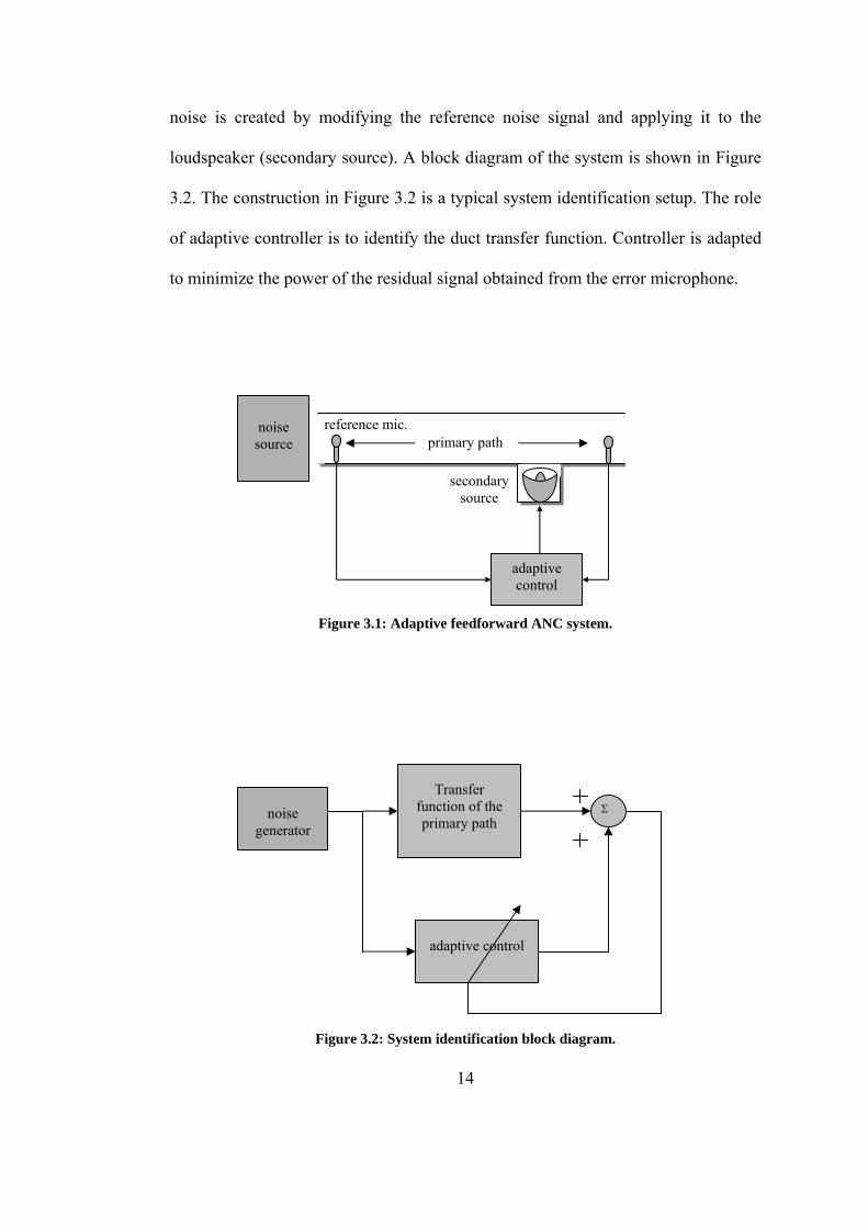
Table 6-1 shows approximate prices of the components and PCB production
in US dollars. Total cost of the system is approximately 127$. PCB production cost
is evaluated for serial production. Production cost of the first PCB is 1200$ and
after that cost of each PCB is 6$/per PCB. This 1200$ have to be added to the cost
50
of the board. For example if 1000 board will be produced 1.2$ have to be added to
the cost of the each board.
Table 6-1: Approximate prices of the components and PCB production in US dollars
TMSVC5416 PROCESSOR 1 25,16 25,16
TLV320AIC20 CODEC 2 7,82 15,64
AM29LV400 FLASH MEMORY 1 27,00 27,00
TPS61006 LDO 1 1,45 1,45
TPS62202 LDO 1 0,68 0,68
TPS62204 LDO 1 0,68 0,68
TPS3307-18 Supervisory 1 1,22 1,22
Oscillator 1 3,45 3,45
Passive Elements 1 40,00 40,00
PCB 1 6,00 6,00
Component placement 1 6,00 6,00
TOTAL 127,28

51
Figure 6.3 XDS510 PP EMULATOR
6.4 Debugging and Emulation
For debugging purposes, an XDS510 parallel port JTAG emulator seen in
Figure 6.3 was supplied by TI. Connection between emulation device and board is
done by use of 14-pin JTAG header on the board. The emulator connects to the PC
from parallel port. TI Code composer studio (CCS) for C5000 IDE software was
also supplied by TI. With the drivers from Spectrum Digital come with the emulator
CCS easily link to the target board.

52
6.5 Software
Prepared software for the DSK implementation was reused with some
modifications.
Codec driver software given in application note SLAA166 [45] from TI
website [46] was used instead of the DSK board support package functions for the
analog input and analog output. This codec driver employs all necessary functions
and sets all necessary interrupt signal to interface the DSP with the codecs.
Noise cancellation and secondary path modelling sections of the code was
not changed.

53
CHAPTER 7
7. EXPERIMENTAL RESULTS AND DISCUSSION
EXPERIMENTAL RESULTS AND DISCUSSION
7.1 Introduction
In this chapter performance test of DSK system, portable system and two
commercially available analog systems will be present.
All systems have been tested with 3 different noise signals, an artificially
generated composition of tones, Bosch PSB 400-2 drill noise and SAAB 340B
propeller plane cabin noise.
The performance of our systems will be compared to those of two
commercially available analog active noise cancellation headphones system-1,
system-2. System1 is ANC headphone of the Bose Corporation. This system is
designed for music listening and it optimal performance is achieved over 100 – 300
Hz band. System2 is headphone of Sennheiser Company. This system is designed
for helicopter pilots and a communication system is integrated into the headphone.
Propeller noise of the helicopter is between 60-80 Hz band and this system is
optimized for this frequency range.

54
In Section 1, DSK system test results, in Section 2, portable board test
results and in Section 3, analog system test results will be given. In the last section,
test results will be discussed.
In all of the following figures related to performance tests, solid blue lines
plot the noise level when ANC system is off and dashed red lines plot the noise
level when the system is on.
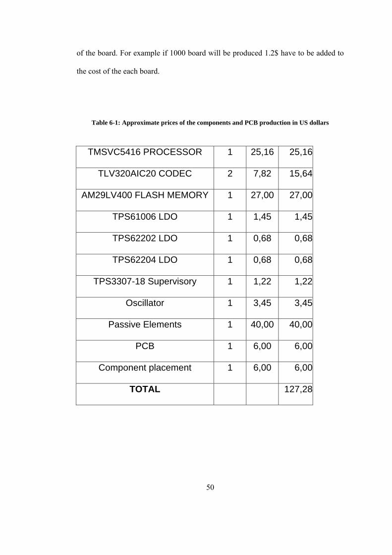
At the last of the chapter, fixed-point Matlab based simulation comparison
of the Fx-LMS and Sign-sign Fx-LMS algorithms will be given and the effect of
dead-zone will be discussed.
7.2 DSK Implementation Experiments
In the tests, 128-tab filters have been used as the secondary path model and
noise cancellation filters. The impulse and frequency magnitude responses of
secondary path model can be seen Figure 7.1.
7.2.1 Tonal Noise Performance Test
In this test, a composition of 5 tones was used. Noise signal had components
at the frequencies of 100, 200, 300, 400, and 500 Hz. Test results of the system is
given in Figure 7.2.
In these tests the DSK system has reached attenuation levels of 17 dB at 100
Hz, 23 dB at 200 Hz, 35 dB at 300 Hz, 45 dB at 400 Hz and 36 dB at 500 Hz.
Attenuation at the signal power reached 27.8 Db.

55
Figure 7.1: Impulse response and magnitude of the frequency response of the secondary path
model.
Figure 7.2: Performance test of DSK system with tones.

56
As seen from the results, digital adaptive system can be effective over the
frequencies between 0-500 Hz intervals.
7.2.2 Drill Noise Performance Test
In this test a recorded Bosch PSB 400-2 drill noise was used. The main
component of this noise is around 450 Hz. Test results of the system is given in
Figure 7.3.
Attenuation level around the main frequency 450 Hz with DSK system was
16 dB and total error signal power attenuation was 4.2 Db.
Figure 7.3: Performance test of DSK system with drill noise.

57
Figure 7.4: Performance test of DSK system with propeller plane cabin noise.
7.2.3 Propeller Plane Cabin Noise Performance Test
In this test a recorded SAAB 340B plane’s cabin noise was used. The main
component of this noise is 80 Hz and it has harmonics at the multiples of 80 Hz
(160, 240, 320, 400 Hz). Test result for DSK system is given in Figure 7.4.
DSK system has reached attenuation levels of 24 dB at 80 Hz, -2 dB at 160
Hz, 14 dB at 240 Hz, 2 dB at 320 Hz and 5 dB at 400 Hz. Total signal power
reduced by 13.4 dB.

58
7.3 Portable System Experiments
7.3.1 Tonal Noise Performance Test
Test result for portable system is given in Figure 7.5.
Figure 7.5: Performance test of portable system with tonal noise.
Attenuation levels with portable board were 13 dB at 100 Hz, 17 dB at 200
Hz, 29 dB at 300 Hz, 24 dB at 400 Hz and 24 dB at 500 Hz. Signal power
attenuation was 22.3 dB.

59
7.3.2 Drill Noise Performance Test
Test result for portable system is given in Figure 7.6.
Attenuation level around the main frequency 450 Hz with portable system
was 13 dB and total error signal power attenuation was 3.7 dB.
Figure 7.6: Performance test of portable system with drill noise.
7.3.3 Propeller Plane Cabin Noise Performance Test
Test result for portable system is given in Figure 7.6.

60
Portable system has reached attenuation levels of 26 dB at 80 Hz, 7 dB at
160 Hz, 14 dB at 240 Hz, 13 dB at 320 Hz and 6 dB at 400 Hz. Total signal power
reduced by 15.1 dB.
7.4 Analog System Experiments
In this test two commercially available headphone active noise control
systems tested. Brands of the system will not be given. The system called as
system-1 is designed for the comfortable music listening and its performance is
optimized in the 200–300 Hz band. System-2 is designed for the helicopter pilots
and thus its performance is optimized below 100 Hz because helicopter motor noise
frequency is around 80 Hz.
Figure 7.7: Performance test of portable system with propeller plane cabin noise

61
7.4.1 Tonal Noise Performance Tests
Test results for system-1 and system-2 are given in Figure 7.8 and Figure
7.9, respectively.
Figure 7.8: Performance test of system-1 headphone with tones.

62
Figure 7.9: Performance test of system-2 headphone with tones.
Attenuation levels with system-1 headphone were 15 dB at 100 Hz, 16 dB at
200 Hz, 13 dB at 300 Hz, 7 dB at 400 Hz and 5 dB at 500 Hz. Signal power
attenuation was 12.2 Db. With system-2 attenuation levels were 19 dB at 100 Hz,
10 dB at 200 Hz, 4 dB at 300 Hz, -3 dB at 400 Hz and -5 dB at 500 Hz. Signal
power attenuation level was 1 dB.
7.4.2 Drill Noise Performance Tests
Test results for system-1 and system-2 are given in Figure 7.10 and Figure
7.11, respectively.

63
Figure 7.10: Performance test of system-1 headphone with drill noise.
Figure 7.11: Performance test of system-2 headphone with drill noise.

64
Attenuation level around the main frequency 450 Hz with system-1 was 7 dB and
total error signal power attenuation was 2.4 Db. These figures are –6 dB and –2.1
dB for system-2.
7.4.3 Propeller Plane Cabin Noise Performance Tests
Test results for system-1 and system-2 are given in Figure 7.12 and Figure
7.13, respectively.
Figure 7.12: Performance test of system-1 headphone with propeller plane cabin noise.

65
Figure 7.13: Performance test of system-2 headphone with propeller plane cabin noise.
System-1 has reached attenuation levels of 14 dB at 80 Hz, 16 dB at 160 Hz,
15 dB at 240 Hz, 12 dB at 320 Hz and 7 dB at 400 Hz. Total signal power reduced
by 12.8 dB. These numbers for system-2 were 15 dB at 80 Hz, 16 dB at 160 Hz, 6
dB at 240 Hz, 0 dB at 320 Hz and -4 dB at 400 Hz. Total signal power reduced by
9.6 dB.
7.5 Discussion of the Tests
In this section, the test results given above will be discussed separately and
finally overall performances will be compared and advantages and disadvantages of
digital system over analog system will be investigated.
Attenuation values of the systems with tonal noise is collected in Table 7-1
Tonal noise performance tests show that the digital systems are effective over the

66
0–500 Hz frequency range but system-1 work effectively in the 100–300 Hz
interval and system-2 works 0–100 Hz interval. From this test, it can be concluded
that the digital systems are very effective on narrow band noise signals at the
frequency range between 0–500 Hz. The main disadvantage of the analog systems
over digital is their fixed small effective ranges.
Table 7-1: Attenuation levels of the systems with tonal noise
100 Hz 200 Hz 300 Hz 400 Hz 500 Hz Total
Attenuation
DSK 17 dB 23 dB 35 dB 45 dB 36 dB 27.8 dB
PORTABLE 13 dB 17 dB 29 dB 24 dB 24 dB 22.3 dB
SYSTEM-1 15 dB 16 dB 13 dB 7 dB 5 dB 12.2 dB
SYSTEM-2 19 dB 10 dB 4 dB -3 dB -5 dB 1 dB
Table 7-2 shows the attenuation levels of systems with drill noise. Analog
systems are not effective with drill noise because the noise signal is not in their
effective range. However, the digital systems reduce the noise at 450 Hz effectively.
Drill noise is a very common noise in day life and an ANC headphone system must
System
Frequency

67
be able to cancel this type of the noise. Because of this fact, digital systems can be
very useful in day life.
In, attenuation levels of the systems with propeller plane cabin noise are
seen.
Table 7-2: Attenuation levels of the systems with drill noise
450 Hz Total Attenuation
DSK 16 dB 4.2 dB
PORTABLE 13 dB 3.7 dB
SYSTEM-1 7 dB 2.4 dB
SYSTEM-2 -6 dB -2.1 dB
The main frequency component of the propeller plane noise is at 80 Hz. In
this frequency, digital systems are the most effective although system-2 is designed
for the noises below 100 Hz. Analog systems is designed to attenuate all frequency
components in their range, however digital systems adapt themselves to the
dominant frequency but in propeller plane noise digital system also attenuates all
System
Frequency

68
frequencies as in analog systems. System-1 is designed to work 100–300 Hz
interval but its performance is very close to the digital system in this interval.
Table 7-3: Attenuation levels of the systems with propeller plane cabin noise.
80 Hz 160 Hz 240 Hz 320 Hz 400 Hz Total
Attenuation
DSK 24 dB -2 dB 14 dB 2 dB 5 dB 13.4 dB
PORTABLE 26 dB 7 dB 14 dB 13 dB 6 dB 15.1 dB
SYSTEM-1 14 dB 16 dB 15 dB 12 dB 7 dB 12.8 dB
SYSTEM-2 15 dB 16 dB 6 dB 0 dB -4 dB 9.6 dB
If DSK and designed portable system are compared, it can be seen that the
DSK system works slightly better than portable system except plane noise. In the
propeller plane noise tests portable system is reached better attenuation values than
the DSK system. Propeller plane noise is a broadband noise. Codec used on the
portable system has higher resolution than the one on the DSK system and this
increases the estimation performance of the system.
System
Frequency

69
7.6 Fixed-point Fx-LMS versus Fixed-point Sign-Sign Fx-LMS
In this section, results of the fixed-point Matlab simulations of Fx-LMS and
sign-sign Fx-LMS algorithms will be given. Comparison of two algorithms in terms
of convergence rate and excess error will be investigated. At the end, the effect of
the dead-zone on the excess error will be discussed. In this section, 16-bit fixed-
point arithmetic is used in all simulations.
7.6.1 Fixed-point Fx-LMS algorithm
Fx-LMS algorithm’s convergence rate and excess error is related to the used
step size of the LMS algorithm. It is expected that when step size of the algorithm is
increased convergence rate and excess error of the algorithm will increase and if
step size is decreased they will decrease. These are true expectations when this
algorithm is implemented with floating-point arithmetic. But fixed-point Fx-LMS
algorithm does not work like floating-point. Because of the information lost in the
divisions, small step size worsens excess error of the algorithm.
A simulation is conducted to observe this problem of the Fx-LMS algorithm.
A 200 Hz sine wave was used as the noise signal and Fx-LMS algorithm was run
for 8000 iterations. In the first case, amplitude of the sine wave is 20000 and in the
second case it is 5000.

70
Figure 7.14:Fx-LMS simulation with sine wave amplitude = 20000.
Figure 7.14 shows learning curves of the algorithm for first case. MSEs after
8000 iterations are 6.4741e+006, 9.7895e+006, 3.4672e+007 for step size values
1/100, 1/200, 1/700, respectively. As expected, convergence rate of the algorithm
decreases with the decreasing step-size but excess error of the algorithm increases.
When noise signal amplitude gets smaller the situation worsens. Figure 7.15 shows
learning curves for small amplitude noise signal. MSEs after 8000 iterations are
6.0953e+006, 1.2500e+007, 1.2500e+007 for step size values 1/100, 1/200, 1/700,
respectively. With small step size values algorithm does not adapt itself. Although
Iteration Number
MSE
71
noise amplitude is small at the second case remaining noise power is the same.
Algorithm does not work effectively.
Because of these problems of the Fx-LMS algorithm in the fixed-point
implementation Sign-Sign Fx-LMS algorithm is used in our study. It is known that
sign-sign LMS algorithm’s convergence rate is very worse and excess error of the
algorithm is larger than standard LMS algorithm. Next part will discuss this fact.
Figure 7.15:Fx-LMS simulation with sine wave amplitude = 5000.
Iteration Number
MSE
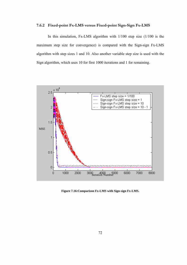
72
7.6.2 Fixed-point Fx-LMS versus Fixed-point Sign-Sign Fx-LMS
In this simulation, Fx-LMS algorithm with 1/100 step size (1/100 is the
maximum step size for convergence) is compared with the Sign-sign Fx-LMS
algorithm with step sizes 1 and 10. Also another variable step size is used with the
Sign algorithm, which uses 10 for first 1000 iterations and 1 for remaining.
Figure 7.16:Comparison Fx-LMS with Sign-sign Fx-LMS.
Iteration Number
MSE

73
Figure 7.16 shows learning curves of the algorithm for first case. Sign–sign
algorithm with step size 1 converges very slowly but has excess error as small as
Fx-LMS algorithm but when step size 10 is used it reaches to the performance of
the Fx-LMS algorithm in terms of convergence rate. Variable step size improves
excess error performance of the algorithm. Variable step size sign-sign Fx-LMS
algorithm works as good as standard Fx-LMS algorithm.
7.6.3 Effect of Dead-Zone to the Sign-Sign Fx-LMS Algorithm
Figure 7.17 shows comparison of the Fx-LMS with step size 1/100 with the
sign-sign Fx-LMS algorithm with step size 10. A dead-zone with magnitude of 4 is
added to the system.
In the figure it can be seen that the dead-zone improves excess error
performance of the system. Sign-Sign Fx-LMS algorithm with dead-zone reaches
performance of the standard Fx-LMS algorithm in terms of both excess error and
convergence rate.

74
Figure 7.17:Comparison Fx-LMS with Sign-sign Fx-LMS with dead-zone.
Figure 7.18 shows the same experiment with noise signal composed of 5
tones (100, 200, 300, 400, 500 Hz). With this noise type, step size of the Fx-LMS
algorithm can be selected very high and it has very good performance. From the red
and green lines, it can be observed that dead-zone mechanism decreases excess mse
performance of the sign-sign algorithm.
Iteration Number
MSE

75
Figure 7.18:Comparison Fx-LMS with Sign-sign Fx-LMS with dead-zone.
From these two experiments, we can conclude that dead-zone mechanism
may increase or decrease excess error performance of the algorithm depending on
the noise signal. Nevertheless, it solves some practical implementation problems of
sign-sign Fx-LMS algorithm and some performance can be sacrificed to solve these
problems.
Iteration Number
MSE

76
7.7 Floating-point Fx-LMS vs Floating-point Sign-Sign Fx-LMS
Sign-sign Fx-LMS algorithm is not an effective solution in the floating-point
implementation. A simulation of the ANC system in floating-point is conducted to
observe performance of the sign-sign algorithm.
Again 200 Hz sine wave is used as the noise signal. The step size of the Fx-
LMS algorithm is chosen as big as possible as in the fixed-point simulation. The
result of the simulation is given in figure Figure 7.19.
In this simulation Fx-LMS algorithm with step size 1/2000 has the best
performance over the two sign-sign algorithms. Maximum possible step size of the
sign-sign algorithm is 1/20000 and even with this step size, it cannot reach
convergence rate of the Fx-LMS algorithm and with this step size, its excess error is
larger. When step size is decreased to 1/50000, its excess error decreases but
convergence rate of the system also decreases. In these two cases, sign-sign
algorithm cannot reach the excess error and convergence rate performance of the
Fx-LMS algorithm.

77
Figure 7.19:Floating-point comparison of Fx-LMS with Sign-sign Fx-LMS.

78
CHAPTER 8
8. CONCLUSION
CONCLUSION
In this thesis, we have aimed to implement ANC system with a fixed-point
DSP for a headphone and to design a battery-powered DSP board to create a
portable headphone ANC system.
In the first part of the thesis, real-time DSP implementation of Fx-LMS
ANC algorithm has been done with TI C5416 DSK board. During the fixed-point
implementations, we have faced up some problems with Fx-LMS algorithm because
of the floating-point nature of the algorithm. One of the problems was the selection
of the step size for stable operation. Step size had to be selected small (very smaller
than 1) to ensure a stable operation but because of the fixed-point division
operation, when step size is selected too small the system stopped adaptation before
it reaches the optimal solution. To solve this problem sign-sign LMS based
algorithm sign-sign Fx-LMS algorithm has been used. Our fixed-point simulations
have shown that sign-sign Fx-LMS algorithm works as good as the Fx-LMS
algorithm. Sign-sign Fx-LMS algorithm is not the only solution of our problems.
Some control statements could be added to the Fx-LMS algorithm. By this way Fx-

79
LMS algorithm could be converted to a suitable algorithm in the fixed-point
implementation but in our simulations and real-time implementations, we have
observed that sign-sign algorithm provided satisfactory performance in our
application. Another justification for the use of sign-sign algorithm is that Fx-LMS
algorithm with control statements would yield more computations than sign-sign
algorithm.
There were some problems with the sign-sign Fx-LMS algorithm described
in Section 4.2. A dead-zone mechanism has been used to prevent these problems.
Sign-sign algorithm with dead-zone mechanism solved the problems of the fixed-
point ANC system. Dead-zone mechanism also improves the excess error
performance of the algorithm.
Some experiments have been conducted with the DSK system and analog
systems to find out performance of the sign-sign Fx-LMS algorithm based ANC
system. These experiments have shown that the digital system is superior to the
analog systems in terms of the noise cancellation performance. Digital system
cancelled all noises between 0–500 Hz band but analog systems worked on a
limited band because of their fixed filtering structure.
In the light of these results, design of a portable system has been decided
and a battery-powered DSP board has been designed and produced. This board
meets the requirements of a portable signal processing application. All the tests
conducted with DSK system have been done with portable system. Our test results
have indicated that a digital headphone ANC system can be considered for

80
commercial purposes. However, for the end-user its tracking performance has to be
improved and stable operation should be studied. In this study, we have mainly
constructed a basis for a prototype but it is not ready to be sold in the market.
8.1 Future Work
Our portable system is not ready to be used out of the laboratory. With
enough financial and human support it can be upgraded to a commercial product for
the market. Some additions to the system can be done. For instance, an audio
system described in [21] or a communication system described in [20] can be
integrated to the system.
Tracking performances of the adaptive digital noise cancellation systems
with fast changing noises are not good compared to the analog systems because
some adaptation time is required for noise cancellation. Some modification on Sign-
sign Fx-LMS algorithm can be considered to improve tracking performance of the
algorithm.

81
REFERENCES
[1] C. M. Harris, Handbook of Acoustical Measurements and Noise Control, 3rd ed. New York: McGraw-Hill, 1991.
[2] L. L. Beranek and I. L. Ver, Noise and Vibration Control Engineering: Principles and Applications. New York: Wiley, 1992.
[3] L. J. Erickson, M. C. Allie, C. D. Bremigan and J. A. Gilbert “Active noise control and specifications for fan noise problems” in Proc. Noise-Con, 1988, pp/ 273-278.
[4] P. Lueg “Process of silencing sound oscillations” U.S. Patent 2,043,416 June 9, 1936.
[5] Sen M. Kuo and Dennis R. Morgan “Active Noise Control: A Tutorial Review” in Proceedings of the IEEE, vol. 87, no. 6, June 1999.
[6] S. J. Elliot and P. A. Nelson “Active Noise Control” IEEE Signal Processing Magazine pp.12-35, Oct. 1993.
[7] Sen M. Kuo and Dennis R. Morgan “Review of DSP Algorithms for Active Noise Control” Proceedings of the 2000 IEEE, International conference on control applications pp. 243- 248 September 25-27 2000.
[8] Sen M. Kuo and Dennis R. Morgan, “Active Noise Control Systems: Algorithms and DSP Implementations”, John Wiley & Sons Inc., New York, 1996.
[9] H. F. Olson and E. G. May, “Electronic sound absorber,” Acoust. Soc. Amer., vol. 25, pp. 1130–1136, Nov. 1953.
[10] R. T. O’Brien, Jr., J.M. Watkins, G. E. Piper, D.C. Bauman “H∞ Active Noise Control of Fan Noise in an Acoustic Duct” in Proceedings of the American Control Conference, pp: 3028-3032, June 2000.
[11] Ian R. Petersen, Hemanshu R. Pota “Experiments in Feedback Control of an Acoustic Duct” Proceedings of the 2000 IEEE, pp. 243- 248 September 25-27 2000.

82
[12] Hisashi Sano, Toshio Inoue, Akira Takahashi, Kenichi Terai, and Yoshio Nakamura “Active Control System for Low-Frequency Road Noise Combined With an Audio System” in IEEE Transactions on speech and audio processing, vol. 9, no. 7, pp: 755-763 October 2001.
[13] Rahmat Shoureshi and Thomas Knurek “Automotive Applications of a Hybrid Active Noise and Vibration Control” in IEEE Control Systems Magazine pp: 72-78 December 1996.
[14] S. M. Hirschs, N. E. Meyer, M. A.Westervelt, P. King, F. J. Li, M. V. Petrova and J. Q. Sun “Experimental Study of Smart Segmented Trim Panels For Aircraft Interior Noise Control” Journal of Sound and vibration (2000) 231(4), pp:1023-1037.
[15] Andre´ Jakob, Michael Moser “Active control of double-glazed windows Part II: Feedback control” Applied Acoustics 64 (2003) pp: 183-196.
[16] J. Landaluze, I. Portilla, J.M. Pagalday, A. Martinez, R. Reyero “Application of active noise control to an elevator cabin” Control Engineering Practice 11 (2003) pp:1423-1431.
[17] Boaz Rafaely “Active Noise Reducing Headset” Proceedings of the First Online Symposium for Electronics Engineers (OSEE), 5 December, 2000.
[18] “Adaptive Active Noise Control for Headphones Using the TMS320C30 DSP” TI Application report spra160 January 1997.
[19] Marek Pawelczyk “Adaptive noise control algorithms for active headrest system” Elsevier Control Engineering Practice.
[20] W. S. Gan, S. M. Kuo “ Integrated active noise control communication headsets” Proceedings of the 2003 International Symposium on Circuits and Systems, 2003 Volume: 4, 25-28 May 2003.
[21] Woon S. Gan and Sen M. Kuo, “An Integrated Audio and Active Noise Controlled Headset”, IEEE Transaction on Consumer Electronics, vol. 48, no: 2, pp. 242-247, May 2002.
[22] Jamil Chaoui, Sebastien de Gregorio, Guillaume Gallissian, Yves Mass “DSP Based Solution for Ambient Noise Reduction in Mobile Phones”, 1999 IEEE International Conference on Acoustics, Speech, and Signal Processing, vol:4, pp: 2391-2394, 15-19 March 1999.
[23] T. Ishimatsu, T. Shimomachi, N. Taguchi “Active vibration control of flexible rotor using electromagnetic damper” 1991 International Conference on Industrial Electronics, Control and instrumentation vol.1, PP:437-442 28 Oct.-1 Nov. 1991.
[24] V. DeBrunner, D. Zhou, M. Ta “Adaptive vibration control of a bridge and heavy truck” Proceedings. IEEE Intelligent Vehicles Symposium, 2003 pp:389-393 9-11 June 2003.

83
[25] Sen M. Kuo, Issa Panahi, Kai M. Chung, Tom Horner, Mark Nadeski and Jason Cyhan “Design of Active Noise Control Systems with the TMS320 Family” SPRA 042 TI Application Report, June 1996.
[26] Jerome C. Couche, Francois Charette, Christopher R. Fuller “Active Control of Automobile Cabin Noise with Advanced Speakers” 136th ASA Meeting, Norfolk, Va, October 13, 1998.
[27] Bose Corporation, “Bose, Worlds Leader in Audio Electronics” www.bose.com, September 21, 2004.
[28] Sennheiser Company, “Sennheiser Worldwide – Evolution Kopf,rer Mikrofon Akustik” www.sennheiser.com, September 13, 2004.
[29] Helmets Integrated Systems, “Helmets Integrated Systems Ltd” www.helmets.co.uk.
[30] Holmco Elektroacuistic, “HOLMCO – Holmberg GmbH & Co. KG ELECTROACOUSTIC”, www.holmco.de/index.html.en, September 15, 2004.
[31] D. R. Morgan, “Analysis of Multiple Correlation Cancellation Loop with a Filter in the Auxiliary Path” IEEE Transaction on ASSP vol. ASSP-28, no: 4, pp. 454-467, August 1980.
[32] B. Widrow, “Adaptive Noise Canceling: Principles and Applications”, Proc. of IEEE vol. 63, no: 12, pp. 1692-1716, Dec. 1975.
[33] Simon Haykin, “Adaptive Filter Theory”, Prentice Hall, 1996.
[34] P. S. R.Diniz, “Adaptive Filtering-Algorithms and Practical Implementation”, Kluwer, 1997.
[35] O. Macchi, “Adaptive Processing”, Wiley, 1995.
[36] Monson H. Hayes, “Statistical Digital Signal Processing and Modeling”, John Wiley & Sons Inc., 1996.
[37] B. Widrow and S. D. Stearns, “Adaptive Signal Processing”, Englewood Cliffs, NJ: Prentice Hall, 1985.
[38] D. Guicking, "A Broadband Active Noise Control System Using a Fast RLS algorithm," Proceedings of the Third International Congress on Air and Structure-borne Sound and Vibration, pp. 1361-1368, 1994.
[39] H.Sano, S.Adachi and H.Kasuya, “Application of a least squares lattice algorithm to active noise control for an automobile”, Trans. of the ASME, J. of Dynamic Systems, Measurement, and Control, Vol.119, pp.318-320, No.2, June 1997.

84
[40] C. H. Rohrs, C. R. Johnson, J. D. Mills, “A Stability Problem in Sign-Sign Adaptive Algorithms”, ICASSP 86, TOKYO, vol 55.18. 1, pp.2999-3001, April 1986.
[41] TMS320C54x DSP CPU and Peripherals TI Reference Set vol. 1 Literature no: SPRU131G, March 2001.
[42] TI Code Composer Studio 'C5416 DSK Tools 2 ('C5416) Help.
[43] TMS320C54x DSP Library Programmer’s Reference, Literature no: SPRU518C, August 2002.
[44] TMS320C54x DSP Mnemonic Instruction Set Reference Set vol. 2 Literature no: SPRU172C, March 2001.
[45] TI Application Report, “TMS320C54x DSP Reference Framework & Device Driver for the TLV320AIC20 HPA Data Converter”, Slaa166, January 2003.
[46] Texas Instruments, “Texas Instruments Welcomes You”, www.ti.com, September 23, 2004.