are exchange rates cointegrated with monetary model in panel data?

International Journal of Finance and EconomicsInt. J. Fin. Econ. 4: 147–154 (1999)

Are Exchange Rates Cointegratedwith Monetary Model in PanelData?

Keun-Yeob Oh*Department of International Management, Chung-Nam National University,Tae-Jon, 305-764, Republic of Korea

The question ‘Does the monetary model explain the exchange rate move-ment?’ is re-examined. Using the simple monetary model, whether or not theexchange rates are cointegrated with the monetary model is tested. Withdata from seven countries during the recent float period, the panel approachgives favorable results for the monetary model. At the same time, there is nocointegration relationship from the bilateral approach. From the results thatthe panel methods provide, with a higher power of testing, it seems thatsome results from previous tests with bilateral rates may become invalid.Copyright © 1999 John Wiley & Sons, Ltd.

KEY WORDS: exchange rate; monetary model; panel cointegration

EXCHANGE RATE AND MONETARYMODEL COINTEGRATION

Previous empirical research for the exchange ratesduring the recent float period found little evidencein support of the hypothesis that the monetarymodel can explain the movement of exchangerates. Meese and Rogoff (1983) found that thesimple monetary model and other variants couldnot beat the random walk model in out-of-sampleforecasting for the short and long run. The predic-tions with monetary models could not give rise tosmaller errors than the random walk model. Theirresults were disappointing to the economists be-cause it could mean that the theoretical economic

models were not useful in forecasting the move-ments of economic variables. A large body ofresearch in the exchange rate field has been dedi-cated to look for a new way to beat the randomwalk model. There are some papers insisting thattheir models may have more predictive powerthan the random walk model, using diverse ap-proach. For example, Diebold and Nason (1990),Engel and Hamilton (1990) and Mark (1995) areamong them.

Turning to literature more directly related tothis paper, the authors have some research investi-gating the cointegration relationship between theexchange rates and monetary model. The outputof Boothe and Glassman (1987) was not rejectingthe null hypothesis of no cointegration betweentwo variables by using German mark (DM) data.Meese (1986) obtained similar results from theGerman mark, British pound and Japanese yen.Other researchers could not obtain the cointegra-tion relationship with the model or some variantsof the model for data set during the recent floating

* Correspondence to: Department of International Management,Chung-Nam National University, Tae-Jon, 305-764, Republic ofKorea. Tel.: +82 42 8215560; fax: +82 42 8235359; e-mail:[email protected]

JEL Code: F30, F31.

Contract/grant sponsor: Korea Research Foundation

CCC 1076–9307/99/020147-08$17.50Copyright © 1999 John Wiley & Sons, Ltd.

K.-Y. Oh148

exchange rates period (see Baillie and Selover,1987). Most of these papers are using the Engle–Granger residual based two-step method forcointegration tests. It is, however, very well-known that the unit root tests used in the two-stepmethods have very low power (see Dickey andFuller, 1979). For example, Hakkio (1986) showed,using simulation, that when the time series datahas a near unit root, it is possible that the tests donot reject the null hypothesis of the unit root. Thismeans that the Engle–Granger two-step methodmay have some problem in detecting cointegrationrelationship from the data sets.

The response of some researchers has been toemploy the Johansen (1988) MLE method. Forexample, MacDonald and Taylor (1991) criticizedprevious testing methods and used this MLEmethod and demonstrated that there is strongsupport for the monetary model as a long runrelationship. Moosa (1994) also used the MLEmethod and included non-tradables as well astradables. He obtained some results supportingcointegration between the exchange rates and themonetary model. The Johansen MLE method,however, also has some problems, even thoughthey have higher testing power. In contrast to theEngle–Granger method, this method is known tooverly support the cointegration relationship (seeCheung and Lai, 1993).

In this paper, the authors employ the panel dataapproach. Pooled panel data sets for economicresearch possess several major advantages overconventional single time series or cross sectionaldata sets. Panel analysis, especially, can providedramatic improvement in the power of unit roottests by increasing the number of observations. Inthe exchange rate research area, a number of re-searchers have turned to these panel data meth-ods, inspired by Levin and Lin (1992) (hereafterLL) and Im et al. (1995) also studied the asymptoticdistribution and small sample properties of panelunit root tests. The panel methods have been oftenapplied to PPP problem. Oh (1996) investigatedthe PPP relation by using the unit root tests of realexchange rates in panel data and obtained favor-able results from the recent float data. Other stud-ies employed this panel approach to analyze theexchange rates and obtained some evidence forPPP (see Wu, 1996; Papell, 1997). Pedroni (1995,1996) studied the properties of cointegration tests

in heterogeneous panels and applied his panelcointegration method to PPP. He found evidenceto support the idea that although ‘weak’ PPP ap-pears to hold, the ‘strong’ form of PPP does not(see Pedroni, 1996).

This paper is going to test whether exchangerates in the long run are cointegrated with themonetary model by using panel data. Further-more, the simple comparison of tests’ power sizewill be illustrated for various observations andindividuals. The authors will demonstrate the lowpower of the unit root tests and how much it canbe improved by using panel data.

Using the simple monetary model, they testwhether or not the exchange rates are cointegratedwith the monetary model. With data from sevencountries during the recent float period, the panelapproach gives favorable results for the monetarymodel and at the same time not having a cointe-gration relationship from the bilateral approach.As the number of countries in the panel data isincreased, they obtain stronger evidence in sup-port of the monetary approach. Because the panelmethods provides a higher power of testing, itseems that some results from previous tests withbilateral rates may become invalid.

MONETARY MODEL, PANEL DATAMETHODS

Exchange Rates and Monetary Model

An exchange rate with simple flexible price modelis reduced to the following form:

et=c1+c2(mt−m t*)−c3(yt−y t*), (1)

where et, mt and yt are the logarithms of exchangerate, money supply and income, respectively. Theasterisks indicate foreign variables. This equationshows that the relative money supply and relativeincome affects on the exchange rates. It is assumedthat there is a PPP relationship between the ex-change rate and two price levels. Of course thereare many forms of monetary model. The authorsemploy Equation (1) because it is the simplest andit seems to be the most appropriate form for thetraditional monetary model.

Copyright © 1999 John Wiley & Sons, Ltd. Int. J. Fin. Econ. 4: 147–154 (1999)

Exchange Rate and Monetary Model Cointegration 149

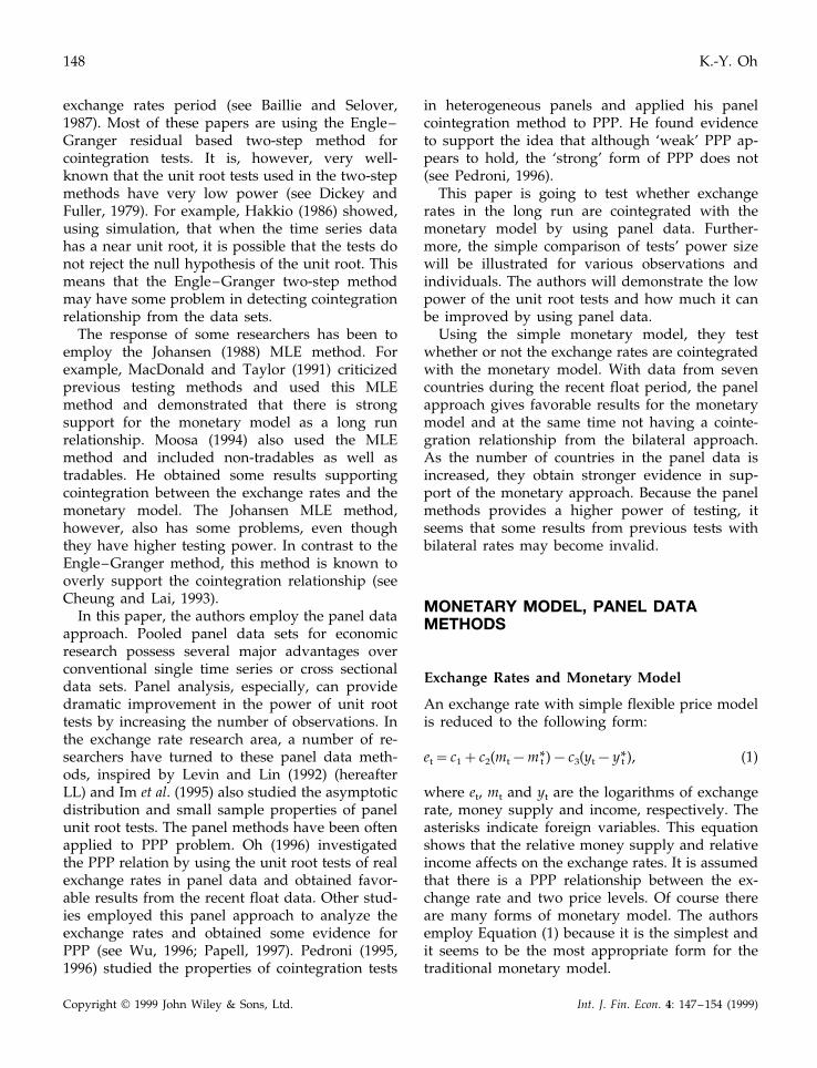
Table 1. Improvement of tests power in panel data methods

N=1 N=2 N=3 N=7Significance level N=10 N=50 N=100

T=22 0.015 0.016 0.033 0.0511% 0.088 0.652 0.948T=90 0.074 0.019 0.392 0.935 0.995 1.000 1.000

T=22 0.064 0.096 0.121 0.2075% 0.258 0.889 0.992T=90 0.272 0.535 0.776 0.995 1.000 1.000 1.000

This table is basically based on the same Monte Carlo simulation as in Oh (1996), but the number ofobservations was changed for the data set.

Panel Data Methods

The authors make use of the ‘Engle–Grangercointegration test’, which consists of two steps.The first step is applying OLS to the Equation (1)and computing the time series of the residual fromthe regression. The second step is applying unitroot tests to the residuals by using the augmentedDickey–Fuller (ADF) test. This procedure will beapplied for the panel data. They apply LL’s panelunit root tests to the second step (see Levin andLin, 1992). (An anonymous referee thankfully re-minded the authors of a recent result. Taylor andSarno (1998) have shown that panel unit root testsmay reject the null hypothesis of joint non-station-arity when just a few of the series are stationaryand not all of them.)

Unit Root Tests versus Cointegration Tests

It is well-known that if critical values of usualADF tests are used, wrong inference could beimplemented in the Engle–Granger cointegrationtest. For the single time series data, the asymptoticdistribution of this two-step test is different fromADF unit root test. This is because the estimationin the first step creates some bias. In panel cointe-gration, fortunately, you do not have this bias (seePedroni, 1995, 1996). For example, Pedroni showedthat ‘the sample moment of the estimated residu-als converges in distribution to those of the trueresiduals’ and the critical values for the statisticare the same whether you use original data orestimated residuals. This property is very differentfrom the usual single cointegration test. Further-more, two-step Monte–Carlo simulation resultsare used to obtain critical values in actual tests,because the finite sample properties are a littledifferent from asymptotic.

Power Improvement in the Panel Tests

Table 1 shows the results of a simulation to checkthe changes in testing power in the panel methods.For this simulation, the following data generatingmethods were used under an alternative hypothe-sis: Yit=0.9Yit−1+wit, where wit are i.i.d. Thistable shows dramatic improvements in testingpower when pooled data were used. The resultsare almost the same feature as those in LL.

THE RESULTS

In this section, the results from the panel data arepresented. The results with a 5% significance levelare reported.

Panel Unit Root Tests for Nominal ExchangeRate

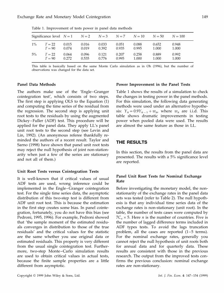
Before investigating the monetary model, the non-stationarity of the exchange rates in the panel datasets was tested (refer to Table 2). The null hypoth-esis is that any individual time series data of theexchange rates is non-stationary (unit root). In thetable, the number of tests cases were computed by7Cn×5. Here n is the number of countries. Five isthe number of lagged difference terms included inADF types tests. To avoid the lags truncationproblem, all the cases are reported (1–5 terms).For the nominal exchange rates, generally youcannot reject the null hypothesis of unit roots bothfor annual data and for quarterly data. Theseresults are consistent with those in the previousresearch. The output from the improved tests con-firms the previous conclusion: nominal exchangerates are non-stationary.


K.-Y. Oh150

Table 2. Unit root test for nominal exchange rate

Number of Number of Quarterly dataAnnual datacases (a)countries

Number of Rejection ratio Rejection ratioNumber of(c/a)rejections (c)(b/a)rejections (b)

35 0 0.000 0 0.0001105 2 0.0192 1 0.095175 53 0.029 0 0.000175 7 0.0404 0 0.000105 6 0.057 05 0.00035 2 0.0576 0 0.000

5 07 0.000 0 0.000

Real Exchange Rates

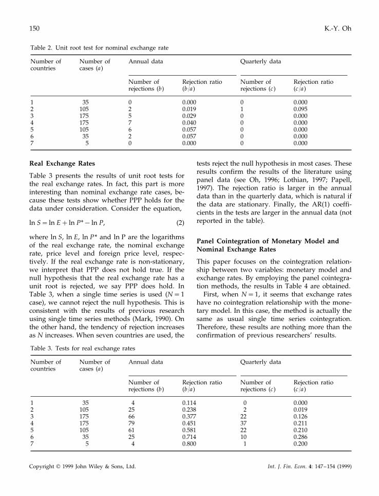
Table 3 presents the results of unit root tests forthe real exchange rates. In fact, this part is moreinteresting than nominal exchange rate cases, be-cause these tests show whether PPP holds for thedata under consideration. Consider the equation,

ln S= ln E+ ln P*− ln P, (2)

where ln S, ln E, ln P* and ln P are the logarithmsof the real exchange rate, the nominal exchangerate, price level and foreign price level, respec-tively. If the real exchange rate is non-stationary,we interpret that PPP does not hold true. If thenull hypothesis that the real exchange rate has aunit root is rejected, we say PPP does hold. InTable 3, when a single time series is used (N=1case), we cannot reject the null hypothesis. This isconsistent with the results of previous researchusing single time series methods (Mark, 1990). Onthe other hand, the tendency of rejection increasesas N increases. When seven countries are used, the

tests reject the null hypothesis in most cases. Theseresults confirm the results of the literature usingpanel data (see Oh, 1996; Lothian, 1997; Papell,1997). The rejection ratio is larger in the annualdata than in the quarterly data, which is natural ifthe data are stationary. Finally, the AR(1) coeffi-cients in the tests are larger in the annual data (notreported in the table).

Panel Cointegration of Monetary Model andNominal Exchange Rates

This paper focuses on the cointegration relation-ship between two variables: monetary model andexchange rates. By employing the panel cointegra-tion methods, the results in Table 4 are obtained.

First, when N=1, it seems that exchange rateshave no cointegration relationship with the mone-tary model. In this case, the method is actually thesame as usual single time series cointegration.Therefore, these results are nothing more than theconfirmation of previous researchers’ results.

Table 3. Tests for real exchange rates

Annual dataNumber of Quarterly dataNumber ofcases (a)countries

Rejection ratioNumber of Rejection ratio Number ofrejections (b) (c/a)(b/a) rejections (c)

4 0.114 0 0.0001 350.238 22 105 25 0.019

220.377 0.126663 17537 0.2114 175 79 0.451

0.210220.581615 10525 0.714 106 0.286354 0.800 17 0.2005



Table 4. Cointegration tests for monetary and nominal exchange rates (annual data)

Number of Quarterly dataNumber of Annual datacountries cases (a)

Rejection ratioNumber of Rejection ratioNumber of(c/a)rejections (b) rejection (c)(b/a)

1 35 8 0.229 3 0.0862 105 62 0.591 29 0.2763 175 144 0.823 83 0.474

175 161 0.920 0.61110745 105 102 0.971 78 0.743

35 0.886311.0006 357 5 5 1.000 5 1.000

Second, the rejection ratio increases as we increasethe number of countries. This seems to tell us thatthe results in the previous single time series dataresearch were due to the low power of their tests.This interpretation is inspired by the fact that thetesting power is greatly improved as more countriesare included.

Third, the tests reject the null more frequently inthe annual data than in the quarterly data. As it isvery well-known, low frequency data show strongertendency towards the mean than high frequencydata, as long as the data are stationary. If the dataare non-stationary, this observation will not appear.

Finally, for the time series of residuals, AR(1)coefficients show that the half life of deviation isapproximately three quarters (not reported in thetable).

Monetary Model and Real Exchange Rates

The cointegration relationship of the monetarymodel is re-examined by using real exchange rates

instead of nominal exchange rates. Even though themonetary theory tells us Equation (1) is appropriate,a large body of literature shows that actual realexchange rate movements are not different from thenominal exchange rates movement (Mark, 1990). Inthe short run, the Dornbusch (1976) model tells usthat the exchange rate is very flexible and prices arepretty sticky. If this is the case, it seems useful tocheck cointegration between real exchange rates andmonetary model (refer to Table 5). The results arevery similar to those in Table 4: (i) the rejection ratiois increasing when more countries are included inthe tests, and (ii) annual data give rise to morerejections.

Figures 1 and 2 explicitly summarize the resultsin this paper. In Figure 1, as the number of countriesin the tests is increased, the test tends to reject thenull hypothesis of non-stationarity of real exchangerates. Meanwhile, for nominal exchange rates thistendency does not exist. In Figure 2, the twovariables, exchange rates and monetary model, seemto be cointegrated from the panel data.

Table 5. Cointegration test using real exchange rates

Annual data Quarterly dataNumber ofNumber ofcountries cases (a)

Rejection ratioNumber ofRejection ratioNumber ofrejection (b) (b/a) (c/a)rejection (c)

0.200 31 35 0.0867300.705 0.286742 105

0.994 903 175 174 0.5140.7311281.0001754 175

88 0.8385 105 105 1.00032 0.9146 35 35 1.000

5 1.000 57 1.0005


K.-Y. Oh152

Figure 1. Ratio of rejection in the unit root tests.

Figure 2. Ratio of rejection in the cointegration tests.



CONCLUSION

This paper investigates whether the exchange rateis cointegrated with the monetary model. From thepanel data for 1973–1995, the results of cointegra-tion are obtained. The cointegrating tendency wasstronger when more countries were included in thepooled data. From the fact that the panel cointegra-tion approach provides great improvements in thetesting power, it seems that some results fromprevious tests with bilateral rates may becomeinvalid.

ACKNOWLEDGEMENTS

This paper was supported by Non-Directed Re-search Fund of Korea Research Foundation andwas benefited from presentation at the 7th Interna-tional Conference of Korean Economic Associationat Pusan Korea and 24th Conference of Academyof Economics and Finance at Laffayette, LA.

APPENDIX A: DATA

For use of standard data, the authors investigatedthe data of the following countries: the US, Canada,Japan, the UK, France, Germany, Switzerland, andItaly, for the period of January 1973–February1995. Data are selected from the International Fi-nancial Statistics CD-ROM (March, 1996 issue).Quarterly data are selected directly from the CD-ROM. To make annual data, the authors averagedthe data by using the RATS. Gauss 3.2 is used as asupplementary program. The following is a list ofthe codes for each data: Exchange rate (nationalcurrency per dollar): AE.ZF, Gross Domestic Pro-duction in 1990 Prices: 99B.RGF, Money (seasonallyadjusted): 34BZF, Consumer prices: 64.ZF. For themissing data, they took proxies as follows: FranceMoney (M1, seasonally adjusted): 34N.CZF, UKMoney (Quasi Money): 35, US Money: M1 (season-ally adjusted): 59MAC.

REFERENCES

Baillie, R. and Selover, D., ‘Cointegration and Models ofExchange Rate and Models of Exchange Rate Determi-

nation’, International Journal of Forecasting, 3 (1987),43–51.

Boothe, P. and Glassman, D., ‘Off the Mark: Lessons forExchange Rate Modeling’, Oxford Economic Papers, 39(1987), 443–57.

Cheung, Y.W. and Lai, K.S., ‘Finite Sample Sizes ofJohansen’s Likelihood Ratio Test for Cointegration’,Oxford Bulletin of Economics and Statistics, 52 (1993),313–27.

Dickey, D. and Fuller, W., ‘Distribution of the Estima-tors for Autoregressive Time Series with a Unit Root’,Journal of American Statistical Association, (1979), 427–31.

Diebold, F. and Nason, J.A., ‘Non-parametric ExchangeRate Prediction?’, Journal of International Economics, 28(1990), 315–32.

Dornbusch, R., ‘Expectations and Exchange Rate Dy-namics’, Journal of Political Economy, 84 (1976), 1161–76.

Engel, C. and Hamilton, J., ‘Long Swings in the Dollar:Are They in the Data and do Markets Know it?’,American Economic Review, 80 (1990), 689–713.

Hakkio, C.S., ‘Does the Exchange Rate follow a RandomWalk? A Monte Carlo Study of Four Tests for aRandom Walk’, Journal of International Money and Fi-nance, 5 (1986), 221–9.

Im, K.-S., Pesaran, M.H. and Shin, Y., ‘Testing for UnitRoots in Dynamic Heterogeneous Panels’, DAE Work-ing Paper No. 9526, University of Cambridge, 1995.

Johansen, S., ‘Statistical Analysis of Cointegrating Vec-tors’, Journal of Economic Dynamics and Controls, 12(1988), 231–54.

Levin, A. and Lin, C.-F., ‘Unit Root Test in Panel Data:Asymptotic and Finite Sample Properties’, UCSD, Dis-cussion Paper 92-23, 1992.

Lothian, J., ‘Multi-country Evidence on the behavior ofPurchasing Power Parity under the Current Float’,Journal of International Money and Finance, 16 (1997),19–35.

MacDonald, R. and Taylor, M., ‘The Monetary Ap-proach to the Exchange Rate: Long Run Relationshipsand Coefficient restrictions’, Economics Letters, 37(1991), 179–85.

Mark, N., ‘Real and Nominal Exchange in the long run:an Empirical Investigation’, Journal of InternationalEconomics, 28 (1990), 115–36.

Mark, N.C., ‘Exchange Rate and Fundamentals: Evi-dence on Long-horizon Predictability’, American Eco-nomic Review, 85 (1995), 201–18.

Meese, R., ‘Testing for Bubbles in Exchange Rate Mar-kets: A Case of Sparkling Rate’, Journal of PoliticalEconomy, 94 (1986), 345–73.

Meese, R. and Rogoff, K., ‘Empirical Exchange RateModels of 1970s: Do They Fit Out of Sample?’, Journalof International Economics, 14 (1983), 3–24.

Moosa, I., ‘The Monetary Model of Exchange Rate Re-visited’, Applied Financial Economics, (1994), 279–87.

Oh, K.-Y., ‘Purchasing Power Parity and Unit Root Testusing Panel Data’, Journal of International Money andFinance, 15 (1996), 405–18.


K.-Y. Oh154

Papell, D.H., ‘Searching for Stationarity: PurchasingPower Parity under the Current Float’, Journal of Inter-national Economics, 43 (1997), 313–32.

Pedroni, P., ‘Fully Modified OLS for HeterogeneousCointegrated Panels and the Case of PurchasingPower Parity’, Indiana University Working Papers inEconomics, 96-020, 1996.

Pedroni, P., ‘Panel Cointegration; Asymptotic and FiniteSample Properties of Pooled Time Series Tests with an

Application to the PPP Hypothesis’, Indiana Univer-sity, 1995.

Taylor, M.P. and Sarno, L., ‘The Behavior of RealExchange Rates During the Post Bretton Woods Pe-riod’, Journal of International Economics, (1998) forth-coming.

Wu, Y., ‘Are Real Exchange Rates Non-stationary? Evi-dence from a Panel Data Test’, Journal of Money Creditand Banking, 28 (1996), 54–63.


are exchange rates cointegrated with monetary model in panel data?

Documents