arc hydro groundwater tutorials - aquaveo - water modeling solutions
TRANSCRIPT
Page 1 of 26 © Aquaveo
ARC HYDRO GROUNDWATER TUTORIALS
Working with MODFLOW Models – Steady State
Arc Hydro Groundwater (AHGW) is a geodatabase design for representing groundwater
datasets within ArcGIS. The data model helps to archive, display, and analyze
multidimensional groundwater data, and includes several components to represent
different types of datasets, including representations of aquifers and wells/boreholes, 3D
hydrogeologic models, temporal information, and data from simulation models. The Arc
Hydro Groundwater Tools help to import, edit, and manage groundwater data stored in
an AHGW geodatabase. The MODFLOW Analyst is a subset of the AHGW Tools that is
used to manage groundwater simulation models based on the MODFLOW code
developed by the United States Geologic Survey. In this tutorial we will review the
MODFLOW Data Model, learn how to import steady state MODFLOW models, and
create map layers from the MODFLOW data.
Currently, MODFLOW Analyst tools support models in MODFLOW 2000 and 2005
format. If you have a different version you can use the USGS utilities to convert your
model to MODFLOW 2000 or 2005 formats.
1.1 Background
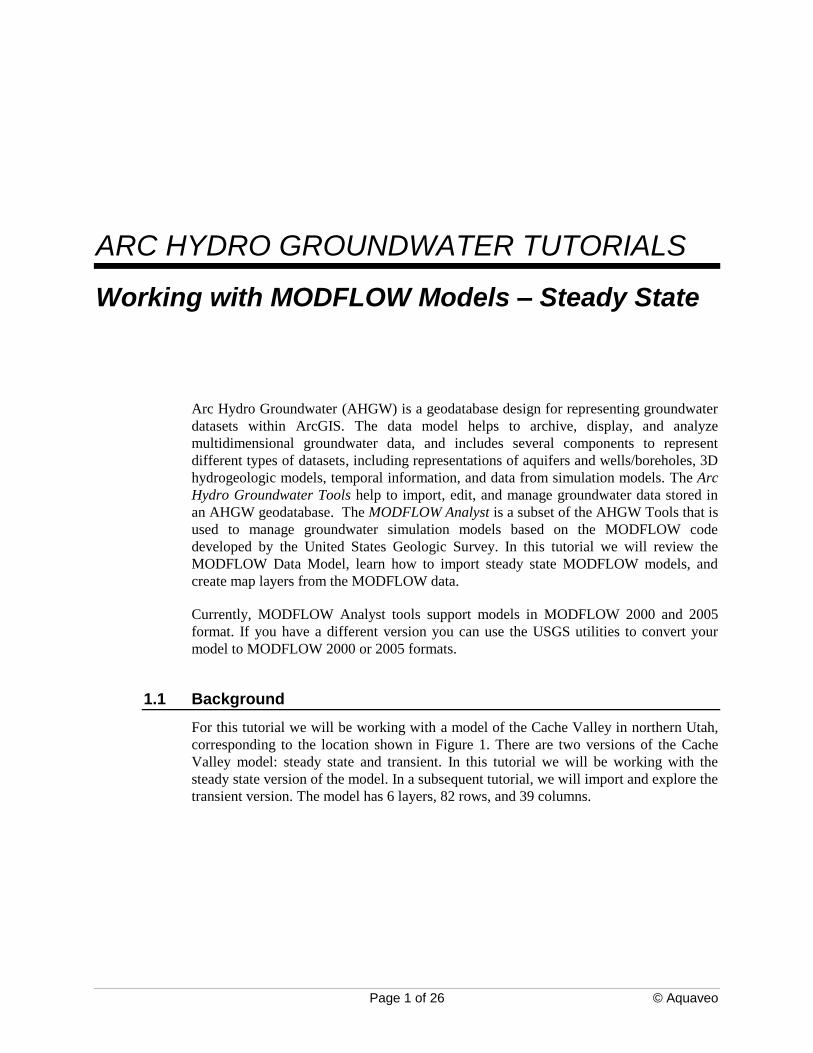
For this tutorial we will be working with a model of the Cache Valley in northern Utah,
corresponding to the location shown in Figure 1. There are two versions of the Cache
Valley model: steady state and transient. In this tutorial we will be working with the
steady state version of the model. In a subsequent tutorial, we will import and explore the
transient version. The model has 6 layers, 82 rows, and 39 columns.
Arc Hydro GW Tutorials Importing MODFLOW Models – Steady State
Page 2 of 26 © Aquaveo
Figure 1 Location of the Cache Valley model.
1.2 Outline
The objective of this tutorial is to introduce the basic components and features of
MODFLOW Analyst. We will complete the following tasks:
1. Review the structure of the MODFLOW Data Model.
2. Import a set of MODFLOW files into ArcGIS.
3. Browse the data in the resulting MODFLOW tables.
4. Generate map layers illustrating array-based MODFLOW data.
5. Generate map layers illustrating list-based MODFLOW stress package data.
6. Import and display a set of MODFLOW solution files.
1.3 Required Modules/Interfaces
You will need the following components enabled in order to complete this tutorial:
Arc View license (or ArcEditor\ArcInfo)
3D Analyst
Arc Hydro Groundwater Tools
AHGW Tutorial Files

Arc Hydro GW Tutorials Importing MODFLOW Models – Steady State
Page 3 of 26 © Aquaveo
The AHGW Tools require that you have a compatible ArcGIS service pack installed.
You may wish to check the AHGW Tools documentation to find the appropriate service
pack for your version of the tools. 3D Analyst is required for the last section of the
tutorial for visualizing 3D features. If you do not have 3D Analyst, you can skip these
parts of the tutorial. The tutorial files should be downloaded to your computer and saved
on a local drive.
2 Getting Started
Before opening our map, let’s ensure that the Arc Hydro and AHGW Tools are correctly
configured.
1. If necessary, launch ArcMap.
2. If necessary, open the ArcToolbox window by clicking on the ArcToolbox icon
.
3. Make sure the Arc Hydro Groundwater Toolbox is loaded. If it is not, add the
toolbox by right-clicking anywhere in the ArcToolbox window and selecting the
Add Toolbox… command. Browse to the top level of the Catalog and then
browse down to the Toolboxes|System Toolboxes directory. Select the toolbox
and select the Open button.
4. Expand the Arc Hydro Groundwater Tools item and then expand the
MODFLOW Analyst toolset to expose the tools we will be using in this tutorial.
We will also be using the MODFLOW Analyst Toolbar. The toolbar contains additional
user interface components not available in the toolbox. If the toolbar is not visible, do the
following:
5. Right-click on any visible toolbar and select the MODFLOW Analyst Toolbar
item.
When using geoprocessing tools you can set the tools to overwrite outputs by default.
To set this option:
6. Open ArcMap/ArcCatalog (if not already open)
7. Select the Geoprocessing | Options... command.
8. Activate the option: “Overwrite the outputs of geoprocessing operations” as
shown in Figure 2.

Arc Hydro GW Tutorials Importing MODFLOW Models – Steady State
Page 4 of 26 © Aquaveo
Figure 2 Setting geoprocessing tools to overwrite outputs by default.
3 Opening the Map
We will begin by importing a map containing some background data for the Cache
model.
1. Select the File| Open command and browse to the location on your local drive
where you have saved the AHGW tutorials. Browse to the modflow
analyst/steady state folder and open the file entitled cache_ss.mxd.
Once the file has loaded you will see a map of Cache Valley in Utah. The file contains a
map layer representing the states in the region. These features will not be used in the
tutorial but are included to provide some context for the MODFLOW model.
Arc Hydro GW Tutorials Importing MODFLOW Models – Steady State
Page 5 of 26 © Aquaveo
4 The MODFLOW Data Model
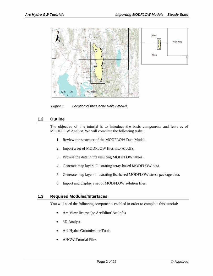
Before importing the MODFLOW files, it is helpful to review the data model we will be
using. The MODFLOW Data Model (MDM) is an extension to the Simulation Feature
Dataset of AHGW (Figure 3). The Simulation feature dataset includes five feature
classes: Boundary, Cell2D, Node2D, Cell3D, and Node3D. Boundary is a polygon
feature class that defines the location of the MODFLOW grid in real world coordinates.
The Cell2D feature class consists of polygons and is used to represent grid cells
associated with two-dimensional simulation models or a single layer of a three-
dimensional model. The Cell3D feature class consists of multipatch objects and is used
to represent three-dimensional cells (primarily for visualization in ArcScene). The
Node2D feature class consists of point features located at the centers of the Cell2D
features and the Node3D feature class consists of 3D point features located at the centers
of Cell3D features. The CellIndex table will be described below.
Boundary
HydroID
HydroCode
Description
OriginX
OriginY
Angle
1
Node2D
HydroID
HydroCode
IJ
Cell2D
HydroID
HydroCode
IJ
Cell3D
HydroID
HydroCode
IJK
Node3D
HydroID
HydroCode
IJK
1
1
1
1
1
*
CellIndex
I
J
K
IJ
IJK
Figure 3 Simulation feature dataset.
The MODFLOW Data Model is built on top of the Simulation feature dataset and it
consists of a series of tables and relationships that can be used to store an entire
MODFLOW simulation within an ArcGIS geodatabase. For example, the tables
associated with the Recharge (RCH) package are shown in Figure 4 and the tables
associated with selected list-based stress packages (River, Well, Drain, etc.) are shown in
Figure 5. The design for the entire MODFLOW Data Model can be viewed at
www.archydrogw.com.

Arc Hydro GW Tutorials Importing MODFLOW Models – Steady State
Page 6 of 26 © Aquaveo
Recharge (RCH)
NRCHOP
RCHVars
Short Int. IJ
SPID
RECH
IRCH
RCHArrays
Long Int.
Long Int.
Double
Long Int.
SPID
AM_RECH
AM_IRCH
RCHArrayMult
Long Int.
Double
Long Int.
Figure 4 Tables for the Recharge package.
List-Based Stress Packages
IJK
SPID
Stage
Cond
Rbot
IFACE
Condfact
SourceID
RIV
Long Int.
Long Int.
Double
Double
Double
Long Int.
Double
Long Int.
IJK
SPID
Q
Qfact
IFACE
SourceID
WEL
Long Int.
Long Int.
Double
Double
Long Int.
Long Int.
IJK
SPID
Elevation
Cond
IFACE
Condfact
SourceID
DRN
Long Int.
Long Int.
Double
Double
Long Int.
Double
Long Int.
IJK
SPID
Shead
Ehead
Shdfact
Ehdfact
SourceID
CHD
Long Int.
Long Int.
Double
Double
Double
Double
Long Int.
IJK
SPID
Bhead
Cond
IFACE
Condfact
SourceID
GHB
Long Int.
Long Int.
Double
Double
Long Int.
Double
Long Int.
IJK1
IJK2
Hydchr
Factor
SourceID
HFB6
Long Int.
Long Int.
Double
Double
Long Int.
Figure 5 Tables for the List-Based stress packages.
In the MODFLOW input files, cells are identified by a combination of three integers
representing the row, column, and layer indices of the cell (I, J, K). Since joins can only
be accomplished using a single field, it is necessary to generate an integer field
corresponding to a unique IJK combination. Furthermore, some MODFLOW input
arrays are fundamentally 2D in nature (Evapotranspiration, Recharge, etc.) and require
an integer identifier corresponding to a unique IJ combination. To facilitate joins and
queries related to the MODFLOW data, the MDM includes a CellIndex table that relates
I, J, and K fields to unique IJ and IJK identifiers. The contents of a CellIndex table for a
MODFLOW grid with three rows, four columns, and two layers is shown in Figure 6a.
The same IJ and IJK indices are organized on a layer-by-layer basis in Figure 6b and 6c.
The IJ and IJK fields of the CellIndex table are populated from the I,J,K values by
starting at a value of one for the cell corresponding to I=1, J=1, K=1, and looping
through the cells in the grid row-by-row within each layer, and incrementing the index.
The IJ index ordering is repeated within each layer.

Arc Hydro GW Tutorials Importing MODFLOW Models – Steady State
Page 7 of 26 © Aquaveo
(A)
(B)
(C)
Red Text = IJ Indices
Blue Text = IJK Indices
Figure 6 Example of a CellIndex table for a grid with 3 rows (I=3), 4 columns (J =4) and 2 layers (K=2).
The Cell2D and Node2D features include an IJ field and the Cell3D and Node3D
features include an IJK field where the IJ and IJK fields are populated using the same
strategy used to populate the CellIndex table. The tables in the MDM containing cell-by-
cell data include either an IJ or IJK field depending on whether it is a 2D array or a 3D
array. The MODFLOW tables can then be joined to the cell and node features using the
CellIndex table (this process will be illustrated later in the tutorial). For example, a map
layer illustrating river cells with point features could be generated by first joining the IJK
field of the RIV table to the IJK field of the CellIndex table. The CellIndex.IJ field of the
resulting temporary table would then be joined to the IJ field of the Node2D feature
class. The values associated with individual grid layers in the resulting map layer can be
displayed using a definition query (“CellIndex.K = 1, CellIndex.K=2, etc.). For 2D
arrays or for models with only one grid layer, the CellIndex table can be bypassed and
the IJ or IJK field of the MODFLOW tables can be joined directly with the IJ field of the
Node2D and Cell2D features since the IJ and IJK values are identical for K=1. Similarly,
joins can be performed directly between IJK-based tables and the Cell3D and/or Node3D
features. Map layers of MODFLOW data associated with cell and node features can be
symbolized and toggled on/off independently from other features in the TOC window in
ArcMap and ArcScene.

Arc Hydro GW Tutorials Importing MODFLOW Models – Steady State
Page 8 of 26 © Aquaveo
5 Importing MODFLOW Files
We are now ready to import MODFLOW files into the geodatabase. Since the
MODFLOW input is divided into a series of files, a typical MODFLOW simulation
consists of 10-20 files. A MODFLOW simulation is imported into ArcGIS in a process
that consists of the following steps:
1. The Import MODFLOW Tables tool is used to read the MODFLOW files,
and load the data from the files into the MDM tables inside a geodatabase.
This tool uses a modified version of MODFLOW that reads the files and
builds the table using the ArcObjects library. Thus, it will work on any
MODFLOW simulation that can be read by MODFLOW.
Tip: Currently, MODFLOW Analyst reads files in MODFLOW 2000 and 2005 format.
If your files are in an earlier format, you may wish to use one of the converter utilities
that can be downloaded from the USGS website.
2. The DIS to Boundary tool reads information related to the grid geometry
from the tables associated with the DIS file and builds a Boundary polygon.
The input to this tool includes the coordinates of the IJ origin of the
MODFLOW grid and the angle of rotation as shown in Figure 7. This
information is necessary to ensure that the MODFLOW model is imported at
the proper location in world coordinate space. The origin coordinates should
be in the same units as the coordinate system associated with the modflow
Feature Dataset created previously.
3. The Create MODFLOW Cell2D tool takes the grid discretization
information in the DIS tables and the Boundary polygon as input and creates
Cell2D features.
4. The Create MODFLOW Node2D tool takes Cell2D features as input and
creates Node2D features.
5. The Create Cell Index Table tool takes the DIS tables as input and creates
the CellIndex table.
6. Optionally, the Create MODFLOW Cell3D and the Create MODFLOW
Node3D tools can be used to create 3D features for use in ArcScene.

Arc Hydro GW Tutorials Importing MODFLOW Models – Steady State
Page 9 of 26 © Aquaveo
φ
Boundary
Origin
Figure 7 Grid origin and angle of rotation used to define the spatial orientation of a MODFLOW Simulation.
In order to simplify this process, the workflow (steps 1-5) has been built into a single
geoprocessing tool called Import Georeferenced MODFLOW Model. We will use this
tool to import the steady state Cache Valley model. One of the inputs for the tool is a
MODFLOW world file (.mwf) which contains information on the model origin, rotation,
and the spatial reference used to georeference the model. Thus, the workflow consists of
two steps:
I. Create a MODFLOW world file.
II. Import the MODFLOW model using the world file.
To create the MODFLOW world file:
1. Double-click on the Create MODFLOW World File tool located in the
MODFLOW Analyst | Import toolset.
2. Enter the following for the origin coordinates:
Origin X: 1334103.5938334
Origin Y: 15392493.413323
Angle of Rotation: 90
3. For the spatial reference, click on the button beside the parameter, and then
select the Import option and browse to the Background.mdb/Background
feature dataset (if you're using older versions of ArcGIS) or choose
NAD_1927_UTM_Zone_12N under Layers on the XY Coordinate System
tab on the Spatial Reference Properties dialog (newer versions of ArcGIS).
4. Specify the output MODFLOW world file location in the “steady state”
directory and name it world_file.mfw.
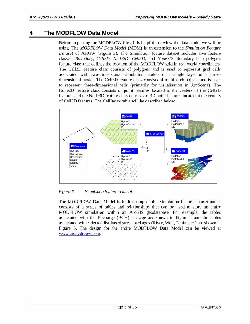
The tool should be populated as shown in Figure 8.
Arc Hydro GW Tutorials Importing MODFLOW Models – Steady State
Page 10 of 26 © Aquaveo
Figure 8 Parameters for the Create MODFLOW World File tool.
5. Select the OK button to execute the tool.
6. Select the Close button when the tool has finished.
Once the tool is run two new text files are created (you can view the content of the files
with any text editor):
world_file.mfw - contains the grid origin and the angle of rotation and a
reference to a text file containing the projection information.
world_file.prj – a text file containing the projection information.
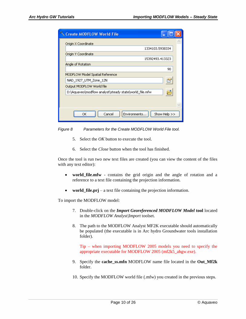
To import the MODFLOW model:
7. Double-click on the Import Georeferenced MODFLOW Model tool located
in the MODFLOW Analyst|Import toolset.
8. The path to the MODFLOW Analyst MF2K executable should automatically
be populated (the executable is in Arc hydro Groundwater tools installation
folder).
Tip – when importing MODFLOW 2005 models you need to specify the
appropriate executable for MODFLOW 2005 (mf2k5_ahgw.exe).
9. Specify the cache_ss.mfn MODFLOW name file located in the Out_Mf2k
folder.
10. Specify the MODFLOW world file (.mfw) you created in the previous steps.

Arc Hydro GW Tutorials Importing MODFLOW Models – Steady State
Page 11 of 26 © Aquaveo
11. Select the steady state folder as the geodatabase location (the tool will
create a new geodatabase in this folder).
12. Specify Cache_SS_MODFLOW for the geodatabase name.
The tool should be populated as shown in Figure 9:
Figure 9 Parameters for the Import Georeferenced MODFLOW Model tool.
After running the tool you should see three new feature layers in the map: Boundary,
Cell2D, and Node2D. A set of tables has also been created in the geodatabase. Check to
see that the MODFLOW tables have been added to the map by selecting the Source tab
in the ArcMap Table of Contents window. If the tables were not added to the map, add
them from the Cache_SS_MODFLOW.mdb geodatabase.
To review the data:
13. Right-click on the Cell2D layer and select the Open Attribute Table
command to view the fields associated with the features. Close the window
when finished. You may wish to repeat this step for the Node2D and
Boundary features.
14. Click on the Source tab at the bottom of the Table of Contents window and
note the list of MODFLOW tables. Right-click on some of the tables and
select the Open command to view the contents.
Before continuing to the next step, we will turn off the display of the features.
15. Toggle off the Cell2D, and Node2D features.

Arc Hydro GW Tutorials Importing MODFLOW Models – Steady State
Page 12 of 26 © Aquaveo
6 Building Active Boundary Polygons
We can now use the Cell2D and Node2D features to create map layers illustrating the
MODFLOW data. To start with, we will use the IBOUND to Polygon tool to create a
map layer containing polygons corresponding to the active region for each of the model
grid layers. This tool uses the IBOUND field in the Basic table and the Cell2D feature
class as input. Active cells have non-zero IBOUND values. To run the tool:
1. Double-click on the IBOUND To Polygon tool in the MODFLOW
Analyst|Views toolset.
2. Click on the down arrow on the right side of the Input Cell2D Features field
and select the Cell2D feature class.
3. Click on the down arrow on the right side of the Input Basic Table field and
select the Basic table.
4. Click on the down arrow on the right side of the IBOUND Array Field field
and select IBOUND.
5. Click on the down arrow on the right side of the Input Index Table field and
select the CellIndex table.
6. Click on the Open button on the right side of the Output IBOUND Polygon
Feature Class field and browse to the Layers feature dataset where the
MODFLOW feature classes were created
(Cache_SS_MODFLOW.mdb\Layers). Enter ActiveBoundary for the name
of the new feature class and select Save.
7. Leave the Layer ID (optional) field blank. Entering an integer in this field
results in an active boundary polygon for the selected layer. If the field is left
blank, an active boundary polygon is created for each layer.
At this point, the settings for the tool should match those shown in Figure 10.

Arc Hydro GW Tutorials Importing MODFLOW Models – Steady State
Page 13 of 26 © Aquaveo
Figure 10 Settings for the IBOUND to Polygon tool.
8. Click OK to launch the tool.
9. When the tool is finished, click the Close button.
You should see a set of overlapping polygons appear, indicating the active regions for
each of the six grid layers.
10. Symbolize the polygons based on the CellIndex_K attribute to better
visualize the active zones of different layers.
7 Using the MODFLOW Grid Layer (K) Filter
The IBOUND to Polygon tool created a feature class containing overlapping polygons
(one for each model layer). One of the fields in the feature class is the “K” field
indicating the index of the grid layer. To view the polygons one at a time, we could apply
a definition query (K=1) to our current map layer using the Layer Properties dialog. The
MODFLOW Analyst toolbar contains a convenient shortcut for creating a definition
query based on the grid layer. To use the filter:
1. Make sure the ActiveBoundary layer is selected in the Table of Contents
window.
2. Locate the K: filter in the MODFLOW Analyst toolbar and
note that the default value is 0. This value results in the display of all layers
at once. Click on the up arrow to the right of the 0 to increment the value to
1.

Arc Hydro GW Tutorials Importing MODFLOW Models – Steady State
Page 14 of 26 © Aquaveo
3. Repeat the previous step to view the active boundary polygon for other
layers.
The K: filter will work for any map layer containing a K field. To apply it to multiple
map layers at once, simply multi-select the map layers in the Table of Contents window
prior to changing the value in the K: filter.
8 Using the Make MODFLOW Feature Layer tool
Next, we will create a map layer of hydraulic conductivity values found in the BCF
package. We will use the Make MODFLOW Feature Layer tool.
The hydraulic conductivity values we will be mapping are stored in the BCFProperties
table. This table also contains other values including transmissivity (Tran), and leakance
(VCont). These values are stored in the BCF Package files as a series of 2D arrays, one
per layer per type. Each record in the table represents a set of values associated with a
particular cell, identified by an IJK value.
1. Double-click on the Make MODFLOW Feature Layer tool in the
MODFLOW Analyst|Views toolset.
2. For the Input Cell/Node Features select Cell2D.
3. For the Input MODFLOW Table select BCFProperties.
4. Select the HY and IJK fields in the MODFLOW Table Fields of Interest.
5. Name the Output MODFLOW Layer HY.
The settings in the tool should now match those shown in Figure 11.

Arc Hydro GW Tutorials Importing MODFLOW Models – Steady State
Page 15 of 26 © Aquaveo
Figure 11 Settings for the Make MODFLOW Feature Layer tool.
6. Click on the OK button.
7. When the tool is finished, click on the Close button.
The HY layer created is a temporary layer in ArcMap.
At this point you should see a new map layer appear in the Table of Contents window
and you should see a new set of cell polygons appear in the display. Next, we will
modify the display of the new HY map layer.
8. Right-click on the HY map layer and select the Properties command.
9. Click on the Symbology tab.

Arc Hydro GW Tutorials Importing MODFLOW Models – Steady State
Page 16 of 26 © Aquaveo
This model uses interpolated hydraulic conductivity, so we will use graduated colors
rather than categories.
10. In the Show: section, click on the Quantities item and select the Graduated
Colors option.
11. In the Value field, select the BCFProperties_HY item.
12. Click on the Classify button.
13. Change the Classes value to 10.
14. Click on the OK button to exit the Classification dialog.
At this point, your selections in the Symbology tab of the Layer Properties dialog should
match those shown in Figure 12.
15. Click on the OK button to exit the Properties dialog.
Figure 12 Settings for the Layer Properties dialog.
The HY map layer illustrates the hydraulic conductivity for all active MODFLOW cells
in layer 1 of the model (other layers in the model have transmissivity values assigned to
the cells).

Arc Hydro GW Tutorials Importing MODFLOW Models – Steady State
Page 17 of 26 © Aquaveo
9 Using the Create MODFLOW Features Tool
Now we will repeat the process of building a map layer but this time we will use the
Create MODFLOW Features tool. This tool is part of MODFLOW Analyst and is built
on top of the Make Query Table tool. It simplifies the process of building a map layer by
automating the construction of the SQL query. We will make a map layer illustrating the
leakance (VCont) values from the BCFProperties table.
1. Double-click on the Create MODFLOW Features tool in the MODFLOW
Analyst|Views toolset.
2. This tool makes map layers out of Cell2D, Node2D, and Node3D features.
The Input Cell/Node Features field is used to specify which type of feature
is to be used in the query. Click on the down arrow for this field and select
the Cell2D feature class.
3. For the Input MODFLOW Table field, click on the down arrow and select
the BCFProperties table.
4. The Additional Filtering Expression field can be used to specify any
additional items to the SQL query that are not part of the standard query. In
this case we will leave it empty.
5. The MODFLOW Table Fields of Interest controls are used to select which of
the fields from the MODFLOW table will be added to the new feature layer.
In this case, we are only interested in the VCont field.
6. The Output MODFLOW Feature Class field is used to specify the name and
location of the new feature class that will be created by the tool. Click on the
Open button to the right of the field and browse to location in the
geodatabase where the MODFLOW features are stored
(Cache_SS_MODFLOW.mdb\Layers). Enter VCont for the name and click
Save.
7. With the Grid Layer (K) filter you can select to map only a specific layer.
Leave the Grid Layer (K) value empty to map all layers.
8. The Only Active Cells toggle is optional. If it is left checked, only active
cells will be used in the query.
9. The MODLOW Tables category includes parameters specifying the Basic,
BasicArrayMult, DISVars, and CellIndex tables. Expand the tab and make
sure the Basic and CellIndex tables are specified correctly.
The settings in the tool should now match those shown in Figure 13.

Arc Hydro GW Tutorials Importing MODFLOW Models – Steady State
Page 18 of 26 © Aquaveo
Figure 13 Settings for the Create MODFLOW Features tool.
10. Click on the OK button.
11. When the tool is finished, click on the Close button.
12. You should see a new VCont layer appear in the Table of Contents. Once
again, you may wish to use the Layer Properties dialog to modify the
symbology so that the VCont values are displayed and use the K: filter in the
MODFLOW Analyst toolbar to isolate and cycle through the grid layers (you
may notice that since the VCont values do not apply to the bottom-most
layer, layer 6 has no VCont values)

Arc Hydro GW Tutorials Importing MODFLOW Models – Steady State
Page 19 of 26 © Aquaveo
You may wish to repeat these steps to build map layers of the following MODFLOW
tables/data using the Cell2D features:
Recharge rates (RCHArrays.RECH)
Evapotranspiration rates (EVTArrays.EVTR)
Bottom elevations (BotmElev.BotmElev)
Starting heads (Basic.STRT)
10 Mapping Drain Package Data
Next, we will use the Create MODFLOW Features tool to generate a map layer
illustrating the locations of the cell-by-cell drain instances used in the Drain package. We
will use the Node2D feature class to display the drain cells.
1. Double-click on the Create MODFLOW Features tool in the MODFLOW
Analyst|Views toolset.
2. Click on the down arrow for the Input Cell/Node Features field and select
the Node2D feature class.
3. For the Input MODFLOW Table field, click on the down arrow and select
the DRN table.
4. In the MODFLOW Table Fields of Interest section, toggle on the following
fields:
Elevation
Cond
5. Click on the Open button to the right of the Output MODFLOW Feature
Class field and browse to location where the MODFLOW features are stored
(Cache_SS_MODFLOW.mdb\Layers). Enter Drains for the name and click
Save.
6. Leave the Only Active Cells toggle selected.
7. The MODLOW Tables tab includes parameters specifying the Basic,
BasicArrayMult, DISVars, and CellIndex table. Expand the tab and make
sure the Basic and CellIndex tales are specified correctly.
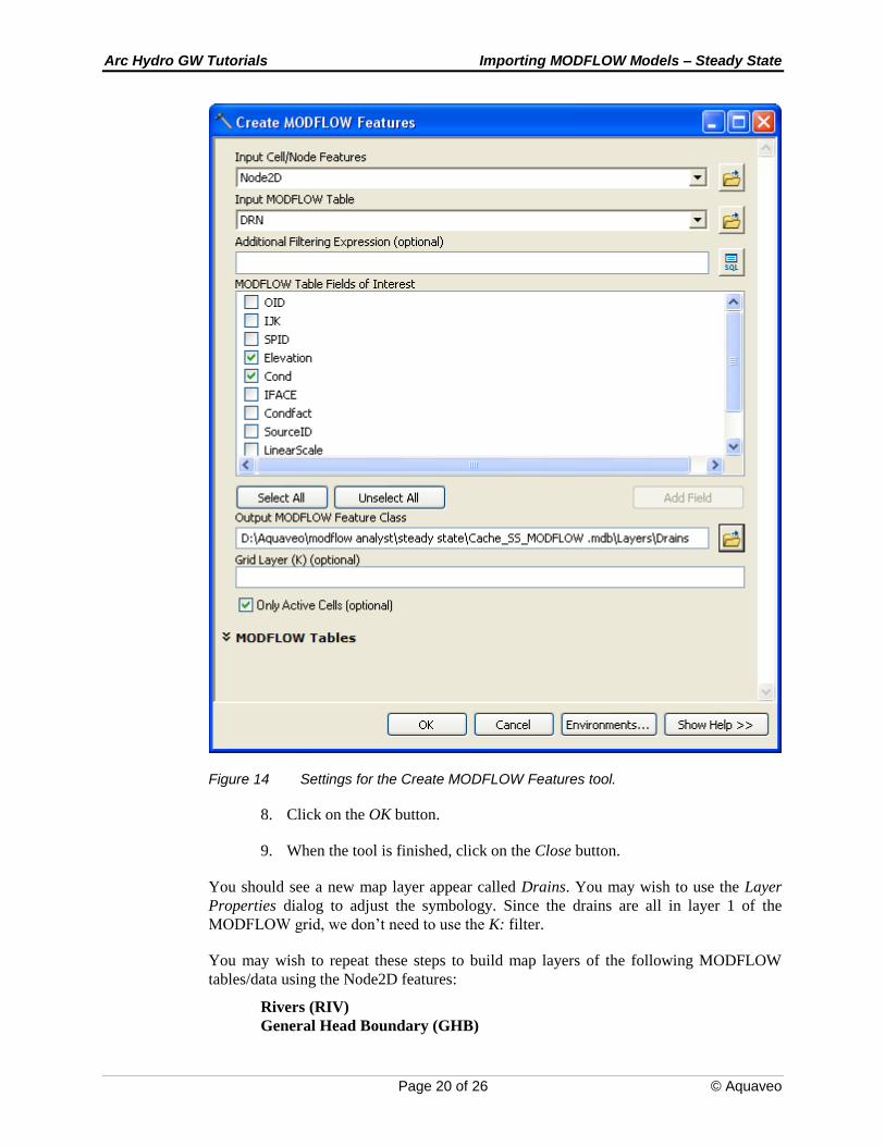
The settings in the tool should now match those shown in Figure 14.
Arc Hydro GW Tutorials Importing MODFLOW Models – Steady State
Page 20 of 26 © Aquaveo
Figure 14 Settings for the Create MODFLOW Features tool.
8. Click on the OK button.
9. When the tool is finished, click on the Close button.
You should see a new map layer appear called Drains. You may wish to use the Layer
Properties dialog to adjust the symbology. Since the drains are all in layer 1 of the
MODFLOW grid, we don’t need to use the K: filter.
You may wish to repeat these steps to build map layers of the following MODFLOW
tables/data using the Node2D features:
Rivers (RIV)
General Head Boundary (GHB)

Arc Hydro GW Tutorials Importing MODFLOW Models – Steady State
Page 21 of 26 © Aquaveo
11 Importing and Displaying Output Data
The output from a MODFLOW simulation includes head, drawdown, and flow data. The
MODFLOW Data Model includes a set of tables for storing this data. To view output
from a MODFLOW simulation, the first step is to import the output files into the tables.
We can then use the Create MODFLOW Features tool to display the output data. To
import the files:
1. Double-click on the Import MODFLOW Output tool in the MODFLOW
Analyst|Import toolset.
2. If necessary, select the appropriate tables for each of the inputs as shown in
Figure 15. Notice that you can import separately (or together) Heads,
Drawdown, and Flow results. In this example we will import heads.
3. Click the OK button.
4. When the tool is finished, click on the Close button.
Figure 15 Settings for the Import MODFLOW Output tool.
When the tool is finished, the display will not change because the tool simply imports the
output data into the appropriate tables. You can view the data imported by opening the
OutputHead table (notice that Heads of 1 represent no value). We will now generate a
map layer of heads.
5. Double-click on the Create MODFLOW Features tool in the MODFLOW
Analyst|Views toolset.

Arc Hydro GW Tutorials Importing MODFLOW Models – Steady State
Page 22 of 26 © Aquaveo
6. Click on the down arrow for the Input Cell/Node Features field and select
the Cell2D feature class.
7. For the Input MODFLOW Table field, click on the down arrow and select
the OutputHead table.
8. In the MODFLOW Table Fields of Interest section, toggle on the Head field:
9. Click on the Open button to the right of the Output MODFLOW Feature
Class box and browse to location in the geodatabase where the MODFLOW
features are stored (Cache_SS_MODFLOW.mdb\Layers). Enter Heads for
the name and click Save.
The settings in the tool should now match those shown in Figure 16.
Figure 16 Settings for the Create MODFLOW Features tool.
10. Click on the OK button.

Arc Hydro GW Tutorials Importing MODFLOW Models – Steady State
Page 23 of 26 © Aquaveo
11. When the tool is finished, click on the Close button.
Next, we will set up the layer symbology:
12. Right-click on the Heads layer and select the Properties command.
13. Click on the Symbology tab.
14. In the Show: section, click on the Quantities item and select the Graduated
Colors option.
15. In the Value field, select the OutputHead_Head item.
16. Click on the Classify button.
17. Change the Classes value to 30.
18. Click on the OK button to exit the Classification dialog.
At this point, your selections in the Symbology tab of the Properties dialog should match
those shown in Figure 17.
19. Click on the OK button to exit the Properties dialog.
Figure 17 Settings for the Layer Properties Dialog.

Arc Hydro GW Tutorials Importing MODFLOW Models – Steady State
Page 24 of 26 © Aquaveo
The cells corresponding to the Heads layer should now be colored. To view the heads
layer by layer, make sure the Heads layer is selected and use the K: filter in the
MODFLOW Analyst toolbar.
12 Creating Cell3D Features
Thus far in the tutorial we have been working with 2D features in ArcMap. For some
models it is useful to generate 3D representations of the MODFLOW data that can be
visualized in ArcScene. This can be accomplished using the Cell3D and Node3D
features. As a final step in the tutorial, we will create a set of Cell3D features and view
them in ArcScene. To complete this step, you must have a 3D Analyst license.
Cell3D features are built from the Boundary polygon and discretization tables containing
the top and bottom elevation arrays. The cells are constructed for active cells only using
the IBOUND values in the Basic table.
We will first need to create the Cell3D feature class using the Catalog Window.
1. Launch the Catalog Window .
2. Navigate to the feature dataset containing the MODFLOW features
(Cache_SS_MODFLOW.mdb\Layers). Right-click on the Layers feature
dataset and select New|Feature Class command.
3. Enter Cell3D for the Name field.
4. Select MultiPatch Features for the Type of features.
5. Select the Next button.
6. Select Finish button.
A new Cell3D feature class is created in the Layers feature dataset.
7. Add the Cell3D feature class to the map and close the Catalog Window.
To create the Cell3D features:
8. Double-click on the Create MODFLOW Cell3D tool in the MODFLOW
Analyst|Features toolset.
9. If not already selected, click on the down arrow to the right of the Input
Boundary Polygon Feature field and select the Boundary feature class.
10. If not already selected, click on the down arrow to the right of the Input
Cell3D Features field and select the Cell3D feature class created in the
previous step.

Arc Hydro GW Tutorials Importing MODFLOW Models – Steady State
Page 25 of 26 © Aquaveo
11. Make sure the Basic Package Tables and Discretization Tables are all
populated.
Figure 18 Settings for the Create MODFLOW Cell3D tool.
12. Click on the OK button.
13. When the tool has finished running (this can take a few minutes), click on
the Close button.
To view the 3D cells we will use ArcScene:
14. Open ArcScene.
15. Add the Cell3D features to the scene using the Add Data command .
You should see a new set of Cell3D features added to the Scene.
16. Save the scene.
To better visualize the cells we will adjust the Scene’s properties:
17. Select View|Scene Prooperties and change the Vertical Exaggeration option
to 20.
18. Select OK to exit the Scene Properties settings.
You can symbolize the features by model layer (K) as shown in Figure 19:

Arc Hydro GW Tutorials Importing MODFLOW Models – Steady State
Page 26 of 26 © Aquaveo
Figure 19 3D view of MODFLOW cells in ArcScene.
13 Conclusion
This concludes the tutorial. Here are some of the key concepts in this tutorial:
The MODFLOW Data Model consists of a set of polygon, point, and multipatch
features and a set of tables containing MODFLOW data. The Data Model
represents a complete MODFLOW model.
A MODFLOW model can be imported into ArcGIS in one step using the Import
Georeferenced MODFLOW Model tool.
The Make Query Table and the Create MODFLOW Features tools can be used
to generate map layers using Cell2D and Node2D features.
For map layers that include features from multiple grid layers, the K: filter can
be used to quickly set up a definition query for a selected grid layer.
MODFLOW solutions can be imported using the Import MODFLOW Output
tool.
Cell3D features can be used to display MODFLOW models in ArcScene.