aquafarm software, j aqua engin 23 (2000)
DESCRIPTION
AquaFarm: simulation and decision support foraquaculture facility design and managementplanningTRANSCRIPT

Seediscussions,stats,andauthorprofilesforthispublicationat:http://www.researchgate.net/publication/222516023
AquaFarm:Simulationanddecisionsupportforaquaculturefacilitydesignandmanagementplanning
ARTICLEinAQUACULTURALENGINEERING·SEPTEMBER2000
ImpactFactor:1.18·DOI:10.1016/S0144-8609(00)00045-5
CITATIONS
34
READS
153
3AUTHORS,INCLUDING:
DougErnst
AquaFarm.com
13PUBLICATIONS215CITATIONS
SEEPROFILE
JohnBolte
OregonStateUniversity
6PUBLICATIONS176CITATIONS
SEEPROFILE
Availablefrom:DougErnst
Retrievedon:04November2015
Aquacultural Engineering 23 (2000) 121–179
AquaFarm: simulation and decision support foraquaculture facility design and management
planning
Douglas H. Ernst a,*, John P. Bolte a, Shree S. Nath b
a Biosystems Analysis Group, Department of Bioresource Engineering, Oregon State Uni6ersity,Gilmore Hall 102B, Cor6allis, OR 97331, USA
b Skillings–Connolly, Inc., 5016 Lacy Boule6ard S.E., Lacy, WA 98503, USA
Received 20 September 1998; accepted 3 September 1999
Abstract
Development and application of a software product for aquaculture facility design andmanagement planning are described (AquaFarm, Oregon State University©). AquaFarmprovides: (1) simulation of physical, chemical, and biological unit processes; (2) simulation offacility and fish culture management; (3) compilation of facility resource and enterprisebudgets; and (4) a graphical user interface and data management capabilities. Theseanalytical tools are combined into an interactive, decision support system for the simulation,analysis, and evaluation of alternative design and management strategies. The quantitativemethods and models used in AquaFarm are primarily adapted from the aquaculture scienceand engineering literature and mechanistic in nature. In addition, new methods have beendeveloped and empirically based simplifications implemented as required to construct acomprehensive, practically oriented, system level, aquaculture simulator. In the use ofAquaFarm, aquaculture production facilities can be of any design and management inten-sity, for purposes of broodfish maturation, egg incubation, and/or growout of finfish orcrustaceans in cage, single pass, serial reuse, water recirculation, or solar-algae pond systems.The user has total control over all facility and management specifications, including siteclimate and water supplies, components and configurations of fish culture systems, fish andfacility management strategies, unit costs of budget items, and production species andobjectives (target fish weights/states and numbers at given future dates). In addition,parameters of unit process models are accessible to the user, including species-specificparameters of fish performance models. Based on these given specifications, aquaculture
www.elsevier.nl/locate/aqua-online
* Corresponding author. Tel.: +1-541-7523917; fax: +1-541-7372082.E-mail address: [email protected] (D.H. Ernst)
0144-8609/00/$ - see front matter © 2000 Elsevier Science B.V. All rights reserved.PII: S0144 -8609 (00 )00045 -5
122 D.H. Ernst et al. / Aquacultural Engineering 23 (2000) 121–179
facilities are simulated, resource requirements and enterprise budgets compiled, and opera-tion and management schedules determined so that fish production objectives are achieved.When facility requirements or production objectives are found to be operationally oreconomically unacceptable, desired results are obtained through iterative design refinement.Facility performance is reported to the user as management schedules, summary reports,enterprise budgets, and tabular and graphical compilations of time-series data for unitprocess, fish, and water quality variables. Application of AquaFarm to various types ofaquaculture systems is demonstrated. AquaFarm is applicable to a range of aquacultureinterests, including education, development, and production. © 2000 Elsevier Science B.V.All rights reserved.
Keywords: Aquaculture; Decision support system; Computer; Design; Modeling; Simulation; Software
1. Introduction
Aquaculture facility design and management planning require expertise in avariety of disciplines and an ability to perform computationally intensive analyses.First, following specification of the physical, chemical, biological, and managementprocesses used to represent a given facility, quantitative procedures are required tomodel these processes, project future facility performance, and determine facilityoperational constraints and capacities. Second, management of large datasets isoften necessary, including facility and management specifications, projected facilityperformance and management schedules, and resource and economic budgets.Finally, design procedures require many calculations, especially when: (1) multiplefish lots and fish rearing units are considered; (2) simulation procedures are used togenerate facility performance and management schedules; (3) alternative design andmanagement strategies are compared; (4) designs are adjusted and optimizedthrough a series of iterative facility performance tests; and (5) production econom-ics are compared over a range of production scales. Such analyses can be used tooptimize production output with respect to required management intensity andresource consumption (or costs) and to explore tradeoffs between fish biomassdensities maintained and fish production throughput achieved (residence time offish in a facility).
To address these challenges, computer software tools for facility design andmanagement planning can embody expertise in aquaculture science and engineeringand serve as mechanisms of technology transfer to education, development, andproduction. In addition, computer tools can assume the burden of data manage-ment and calculation processing and thereby reduce the workload of design andplanning analyses. A current listing and description of software for aquaculturesiting, planning, design, and management is available on the Internet (Ernst, 1998).Much of this software falls under the general heading of decision support systems(Sprague and Watson, 1986; Hopgood, 1991), in which quantitative methods andmodels, rule-based planning and diagnostic procedures (expert systems), and data-bases are packaged into interactive software applications. The application ofdecision support systems to aquaculture is relatively recent and has been preceded
123D.H. Ernst et al. / Aquacultural Engineering 23 (2000) 121–179
by the development of simulation models for research purposes. Foretelling thesetrends, decision support systems have been developed for agriculture for purposesof market analysis, selection of crop cultivars, crop production, disease diagnosis,and pesticide application.
The purpose of this paper is to provide an overview of the development andapplication of AquaFarm (Ver. 1.0, Microsoft Windows®, Oregon State Univer-sity©). AquaFarm is a simulation and decision support software product for thedesign and management planning of finfish and crustacean aquaculture facilities(Ernst, 2000b). Major topics in this discussion are: (1) the division of aquacultureproduction systems into functional components and associated models, includingunit processes, management procedures, and resource accounting; and (2) theflexible reintegration of these components into system-level simulation models anddesign procedures that are adaptable to various aquaculture system types andproduction objectives. To provide this overview at a reasonable length, methodsand models of physical, chemical, and biological unit processes used in AquaFarmare presented as abbreviated summaries in an appendix to this paper. The appendixis organized according to domain experts and unit processes. Example applicationsof AquaFarm to typical design and planning problems are provided but rigorouscase studies are beyond the scope of this paper. Completed and ongoing calibrationand validation procedures for AquaFarm are discussed.
2. AquaFarm development
The aquaculture science and engineering literature was applicable to the develop-ment of AquaFarm through three major avenues. First, studies concerned withaquaculture unit processes and system performance provided models and modelingoverviews for a wide range of physical, chemical, and biological unit processes andsystem types (Chen and Orlob, 1975; Muir, 1982; Bernard, 1983; Allen et al., 1984;James, 1984; Svirezhev et al., 1984; Cuenco et al., 1985a,b,c; Fritz, 1985;Tchobanoglous and Schroeder, 1985; Cuenco, 1989; Piedrahita, 1990; Brune andTomasso, 1991; Colt and Orwicz, 1991b; McLean et al., 1991; Piedrahita, 1991;Weatherly et al., 1993; Timmons and Losordo, 1994; Wood et al., 1996; Piedrahitaet al., 1997). Additional methods and models were newly developed for AquaFarm,including empirically based simplifications, as required to achieve comprehensivecoverage of aquaculture system modeling while avoiding excessive levels of com-plexity and input data requirements. AquaFarm is primarily based on mechanisticprinciples, with empirical components added as necessary to support practicallyoriented design and management analyses for a wide range of users.
A second area of useful literature were studies that provided methods and resultsof aquaculture production trials that could be used for the calibration andvalidation of unit process and fish performance models. These studies consistedmainly of technical papers, plus a few published databases, and are cited as they areused in this paper. Finally, papers reporting software development for end usershave introduced computerized analysis tools and decision support systems to
124 D.H. Ernst et al. / Aquacultural Engineering 23 (2000) 121–179
aquaculture educators, developers, and producers (Bourke et al., 1993; Lannan,1993; Nath, 1996; Leung and El-Gayar, 1997; Piedrahita et al., 1997; Schulstad,1997; Wilton et al., 1997; Stagnitti and Austin, 1998). These reported softwareapplications range widely in their internal mechanisms and intended purpose. Thesoftware POND (Nath et al., 2000) is most similar to AquaFarm and someprogram modules have been jointly developed.
In the development of AquaFarm, it was desired to maintain a practical balancebetween the responsibilities required from users and the analytical capacity pro-vided by AquaFarm. These objectives are somewhat opposed, and a considerablelevel of user responsibility was found necessary to achieve desired levels of analysis.User responsibilities required in the use of AquaFarm consist of facility specifica-tions, model parameters, and decisions regarding alternative facility designs andmanagement strategies. Facility specifications include items such as facility location(for generated climates) or climatic regimes (for file-based climates), source watervariables, components and configurations of water transport, water treatment, andfish culture systems, management strategies, and production objectives. Whileapproximate environmental conditions, typical facility configurations, and typicalmanagement strategies can be provided by AquaFarm, it is not possible to avoiduser responsibility for these site-specific variables. In contrast, model parameters forpassive unit processes (e.g. passive heat and gas transfer and biological processes)are ideally independent of site-specific conditions, given the use of sufficientlydeveloped models. Validated, default values are provided for all parameters.However, due to the necessity of simplifying assumptions and aggregated processesin aquacultural modeling, model parameters may be dependent on site-specificconditions to some degree (Svirezhev et al., 1984). Thus, model parameters forpassive unit processes have been made user accessible for any necessary adjustment.Finally, while the purpose of AquaFarm is to support design and managementdecisions, these decisions must still be made by the user. As a result, some level ofuser responsibility cannot be avoided regarding the underlying processes impactingsystem performance and implications of alternative decisions on facility perfor-mance and economics. Possible methods to alleviate user responsibilities arediscussed in the conclusion to this paper.
AquaFarm was developed to support a wide range of extensive and intensive,fishery-supplementation and food-fish aquaculture facilities, and a wide range ofuser perspectives (e.g. educators, developers, and producers), within a single soft-ware application. Differing analytical needs of these various systems and users havebeen addressed through an adaptable user interface. An alternative strategy wouldhave been the development of separate software applications for each major type ofaquaculture, type of user, and user knowledge level. The development approachused was chosen to avoid requirements for redundant programming, given the largeoverlap in analytical methods, simulation processing, graphical interface, and datamanagement requirements over the range of aquaculture system types and analyti-cal perspectives. In addition, some aquaculture system types are not easily catego-rized, for example intensive tank-based recirculation systems characterized bysignificant levels of phytoplankton and semi-intensive pond-based systems usingrecirculation systems for phytoplankton management.
125D.H. Ernst et al. / Aquacultural Engineering 23 (2000) 121–179
AquaFarm is a stand-alone computer application, programmed in BorlandC+ +® and requiring a PC-based Microsoft Windows® operating environment.The C+ + computer language was chosen for its popularity, portability, availabil-ity of software developer tools, compatibility with the chosen graphical userinterface (Microsoft Windows®), and support of object oriented programming(OOP; Budd 1991; Nath et al., 2000). According to OOP methods, all componentsof AquaFarm are represented as program ‘objects’. These objects are used torepresent abstract entities (e.g. dialog box templates) and real world entities (e.g.fish rearing units) and are organized into hierarchical structures. Each objectcontains data, local and inherited methods, and mechanisms to communicate withother objects as needed. The modular, structured program architecture supportedby OOP is particularly suited to the development of complex system models such asAquaFarm.
3. AquaFarm design procedure
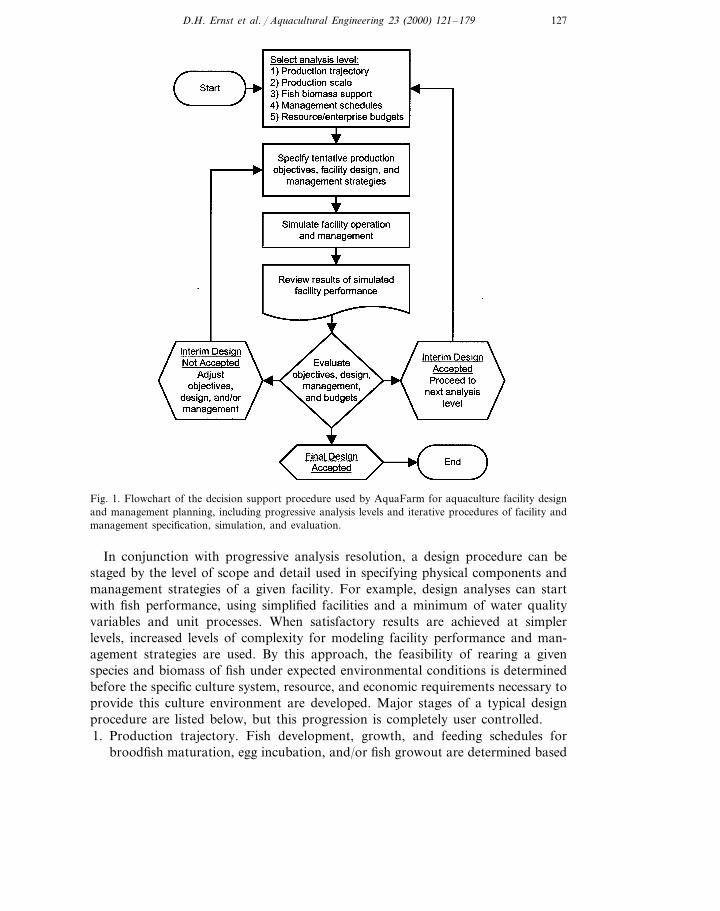
AquaFarm supports interactive design procedures, utilizing progressive levels ofanalysis complexity, simulation based analyses, and iterative design refinement(James, 1984e). These procedures are used to develop design and managementspecifications, until production objectives are achieved or are determined to bebiologically or practically infeasible. This decision making process is user directedand can be used to design new systems or determine production capacities forexisting systems. The analysis resolution level (Table 1) is set so that the complexityof design analyses is matched to levels appropriate for the type of aquaculturesystem and stage of the design procedure. This is accomplished by user control overthe particular variables and processes considered in a given simulation. Forexample, dissolved oxygen can be ignored or modeled as a function of one or moresources and sinks, including water flow, passive and active gas transfer, fishconsumption, and bacterial and phytoplankton processes. Major steps of a typicaldesign procedure are listed below and flow charted in Fig. 1. A summary of inputand output data considered by AquaFarm is provided in Table 2.1. Resolution. An analysis resolution level is selected that is compatible with the
type of facility and stage of the design procedure.2. Specification. Facility environment, design, and management specifications are
established, based on known and tentative information.3. Simulation. The facility is simulated to generate facility performance summaries
and operation schedules over the course of one or more production seasons.4. Evaluation. Predicted facility performance and operation are reviewed and
evaluated, using summary reports, tabular and graphical data presentation,management logs, and enterprise budgets.
5. Iteration. As necessary, facility design, management methods, and/or produc-tion objectives are adjusted so that production objectives and other desiredresults are achieved (go to step 1 or 2).
126 D.H. Ernst et al. / Aquacultural Engineering 23 (2000) 121–179
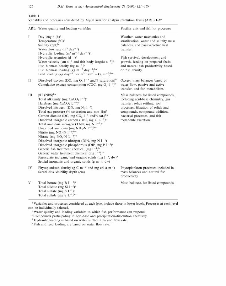
Table 1Variables and processes considered by AquaFarm for analysis resolution levels (ARL) I–Va
ARL Facility unit and fish lot processesWater quality and loading variables
Day length (h)b Weather, water mechanics andITemperature (°C)b stratification, water and salinity massSalinity (ppt)b balances, and passive/active heatWater flow rate (m3 day−1) transfer.Hydraulic loading (m3 m−2 day−1)d
Fish survival, development andHydraulic retention (d−1)b
growth, feeding on prepared feeds,Water velocity (cm s−1 and fish body lengths s−1)b
and natural fish productivity basedFish biomass density (kg m−3)b
on fish density.Fish biomass loading (kg m−3 day−1)b,e
Feed loading (kg day−1 per m3 day−1=kg m−3)b,e
II Dissolved oxygen (DO, mg O2 l−1 and% saturation)b Oxygen mass balances based onwater flow, passive and activeCumulative oxygen consumption (COC, mg O2 l−1)b
transfer, and fish metabolism.
Mass balances for listed compounds,III pH (NBS)b,c
including acid-base chemistry, gasTotal alkalinity (mg CaCO3 l−1)c
Hardness (mg CaCO3 L−1)c transfer, solids settling, soilDissolved nitrogen (DN, mg N2 l−1) processes, filtration of solids andTotal gas pressure (% saturation and mm Hg)b compounds, compound addition,
bacterial processes, and fishCarbon dioxide (DC, mg CO2 l−1 and% sat.)b,c
Dissolved inorganic carbon (DIC, mg C L−1)c metabolite excretionTotal ammonia nitrogen (TAN, mg N l−1)c
Unionized ammonia (mg NH3-N l−1)b,c
Nitrite (mg NO2-N l−1)b,c
Nitrate (mg NO3-N L−1)b
Dissolved inorganic nitrogen (DIN, mg N l−1)Dissolved inorganic phosphorous (DIP, mg P l−1)c
Generic fish treatment chemical (mg l−1)b
Generic water treatment chemical (mg l−1) b
Particulate inorganic and organic solids (mg l−1, dw)b
Settled inorganic and organic solids (g m−2, dw)
IV Phytoplankton processes included inPhytoplankton density (g C m−3 and mg chl-a m–3)mass balances and natural fishSecchi disk visibility depth (cm)productivity
Total borate (mg B L−1)cV Mass balances for listed compoundsTotal silicate (mg Si L–1)c
Total sulfate (mg S L–1)c
Total sulfide (mg S L–1)b,c
a Variables and processes considered at each level include those in lower levels. Processes at each levelcan be individually selected.
b Water quality and loading variables to which fish performance can respond.c Compounds participating in acid-base and precipitation-dissolution chemistry.d Hydraulic loading is based on water surface area and flow rate.e Fish and feed loading are based on water flow rate.
127D.H. Ernst et al. / Aquacultural Engineering 23 (2000) 121–179
Fig. 1. Flowchart of the decision support procedure used by AquaFarm for aquaculture facility designand management planning, including progressive analysis levels and iterative procedures of facility andmanagement specification, simulation, and evaluation.
In conjunction with progressive analysis resolution, a design procedure can bestaged by the level of scope and detail used in specifying physical components andmanagement strategies of a given facility. For example, design analyses can startwith fish performance, using simplified facilities and a minimum of water qualityvariables and unit processes. When satisfactory results are achieved at simplerlevels, increased levels of complexity for modeling facility performance and man-agement strategies are used. By this approach, the feasibility of rearing a givenspecies and biomass of fish under expected environmental conditions is determinedbefore the specific culture system, resource, and economic requirements necessary toprovide this culture environment are developed. Major stages of a typical designprocedure are listed below, but this progression is completely user controlled.1. Production trajectory. Fish development, growth, and feeding schedules for
broodfish maturation, egg incubation, and/or fish growout are determined based
128 D.H. Ernst et al. / Aquacultural Engineering 23 (2000) 121–179
on initial and target fish states. Environmental quality concerns are limited towater temperature and day length, and unit processes are limited to water flowand heat transfer.
2. Production scale. Required water area and volume requirements for fish rearingunits are determined, based on initial and target fish numbers, managementmethods, and biomass density criteria. Natural fish productivity, if considered,is a function of fish density only.
3. Biomass support. Based on fish feed and metabolic loading, facility watertransport and treatment systems are constructed to provide fish rearing unitswith required water flow rates and water quality. The particular variables andunit processes considered depend on the type of facility. Natural fish productiv-ity, if considered, is a function of fish density and primary productivity.
4. Management schedules. Fish and facility management methods and schedulesare finalized, including operation of culture systems, fish lot handling, and fishnumber, weight, and feeding schedules.
5. Resource budgets. Resource and enterprise budgets are generated and reviewed.
Table 2Summary of input specification and output performance data considered by AquaFarm
Input specification dataPossible adjustment of parameters for passive physical, chemical, and biological unit processes and
fish performance modelsFacility location (or climate data files), optional facility housing and controlled climate, and water
quality and capacity of source water(s)Configuration of facility units for facility water transport, water treatment, and fish culture systemsSpecifications of individual facility units, including dimensions, elevations and hydraulics, soil and
materials, housing, and water transport and treatment processesFish species, fish and facility management strategies, and production objectives (target fish
weights/states and numbers at given future dates)Unit costs for budget items and additional budget items not generated by AquaFarm
Output performance dataFish number and development schedules for broodfish maturation and egg incubationFish number, weight, and feed application schedules for fish growout, including optional
consideration of fish weight distributions within a fish lotFish rearing unit usage and fish lot handling schedulesTabular and graphical compilations of time-series data for fish performance variables, reported on
a fish population and individual fish lot basis, including fish numbers and state, bioenergetic andfeeding variables, and biomass loading and water quality variables
Tabular and graphical compilations of time-series data for facility performance variables, reportedon a facility and individual facility unit basis, including climate, water quality, fish and feedloading, water flow rates and budgets, compound budgets, process rates, resource use, wasteproduction, and water discharge
Fish production reports, resource use summaries, and enterprise budgets
129D.H. Ernst et al. / Aquacultural Engineering 23 (2000) 121–179
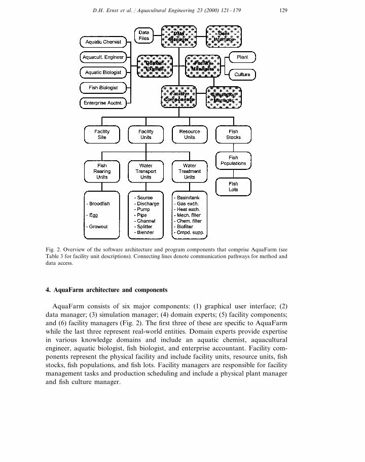
Fig. 2. Overview of the software architecture and program components that comprise AquaFarm (seeTable 3 for facility unit descriptions). Connecting lines denote communication pathways for method anddata access.
4. AquaFarm architecture and components
AquaFarm consists of six major components: (1) graphical user interface; (2)data manager; (3) simulation manager; (4) domain experts; (5) facility components;and (6) facility managers (Fig. 2). The first three of these are specific to AquaFarmwhile the last three represent real-world entities. Domain experts provide expertisein various knowledge domains and include an aquatic chemist, aquaculturalengineer, aquatic biologist, fish biologist, and enterprise accountant. Facility com-ponents represent the physical facility and include facility units, resource units, fishstocks, fish populations, and fish lots. Facility managers are responsible for facilitymanagement tasks and production scheduling and include a physical plant managerand fish culture manager.
130 D.H. Ernst et al. / Aquacultural Engineering 23 (2000) 121–179
4.1. User interface and data management
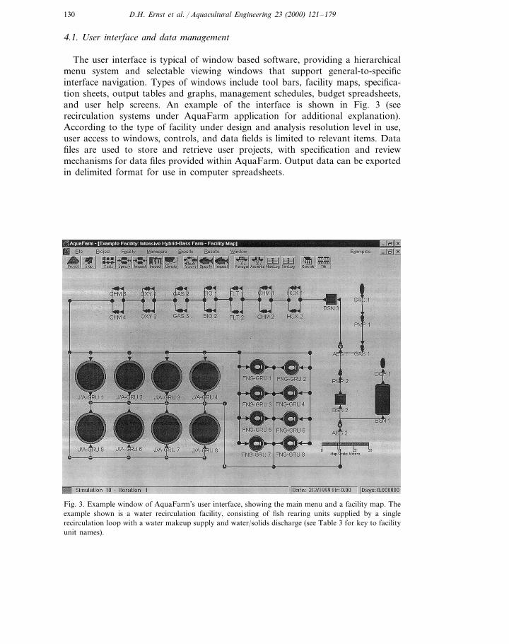
The user interface is typical of window based software, providing a hierarchicalmenu system and selectable viewing windows that support general-to-specificinterface navigation. Types of windows include tool bars, facility maps, specifica-tion sheets, output tables and graphs, management schedules, budget spreadsheets,and user help screens. An example of the interface is shown in Fig. 3 (seerecirculation systems under AquaFarm application for additional explanation).According to the type of facility under design and analysis resolution level in use,user access to windows, controls, and data fields is limited to relevant items. Datafiles are used to store and retrieve user projects, with specification and reviewmechanisms for data files provided within AquaFarm. Output data can be exportedin delimited format for use in computer spreadsheets.
Fig. 3. Example window of AquaFarm’s user interface, showing the main menu and a facility map. Theexample shown is a water recirculation facility, consisting of fish rearing units supplied by a singlerecirculation loop with a water makeup supply and water/solids discharge (see Table 3 for key to facilityunit names).
131D.H. Ernst et al. / Aquacultural Engineering 23 (2000) 121–179
4.2. Domain experts
Domain experts provide expertise in aquaculture science and engineering in theform of quantitative methods and models. These methods consist of property,equilibrium, and rate calculations of physical, chemical, and biological unit pro-cesses and their rules of application. These methods are used to calculate terms infacility-unit and fish-lot state equations and to support management analyses. Thedocumentation required to fully describe these methods is not possible within thesize constraints of this paper. Methods of the aquatic chemist, aquaculturalengineer, aquatic biologist, and fish biologist are summarized in the appendix, andthe enterprise accountant is described below.
4.2.1. Enterprise accountantThe enterprise accountant is responsible for compiling enterprise budgets, which
are used to quantify net profit or loss over specified production periods (Meade,1989; Engle et al., 1997). Enterprise budgets are particularly appropriate forcomparing alternative facility designs, in which partial budgets are utilized thatfocus on cost and revenue items significantly influenced by proposed changes.Additional financial statements (e.g. cash flow and net worth), economic feasibilityanalyses (e.g. net present value and internal rate of return), and market analyses arerequired for comprehensive economic analyses (Shang, 1981; Allen et al., 1984;Meade, 1989) but are not supported by AquaFarm.
Cost items (e.g. fish feed) and revenue items (e.g. produced fish) can be specifiedand budgets can be summarized according to various production bases, timeperiods, and cost types. Item and budget bases include per unit production area, perunit fish production, and per total facility. Item and budget periods include daily,annual, and user specified periods. Cost types include fixed and variable costs, asdetermined by their independence or dependence on production output, respec-tively. Fixed costs include items such as management, maintenance, insurance,taxes, interest on owned capital (opportunity costs), interest on borrowed capital,and depreciation for durable assets with finite lifetimes. Variable costs include itemssuch as seasonal labor, energy and materials, equipment repair, and interest onoperational capital.
Enterprise budgets are built by combining simulation-generated and user-spe-cified cost and revenue items. Simulation generated items are those directly associ-ated with aquaculture production and therefore predictable by AquaFarm, e.g.facility units, energy and material consumption, and produced fish and wastes.AquaFarm determines total quantities for these items (numbers of units), but theuser is responsible for unit costs and other specifications (e.g. interest rates, usefullives, and salvage values). User specified items include additional cost and revenueitems outside the scope of AquaFarm, e.g. supplies, equipment, facility infrastruc-ture, and labor. For user specified items that are scalable, the use of unitized costbases (i.e. per unit production area or production output) alleviates the need tore-specify item quantities when working through multiple design scenarios. Thebudget is shown in spreadsheet format for the selected budget basis and period,
132 D.H. Ernst et al. / Aquacultural Engineering 23 (2000) 121–179
with cost and revenue items totaled and net profit or loss calculated. Net profitvalues can also be used as net return values to cost items that are not included inthe budget, e.g. net return to land, labor, and/or management.
4.3. Facility site, facility units, and resource units
An aquaculture facility is represented by a facility site, facility units, and resourceunits. A facility site consists of a given location (latitude, longitude, and altitude),ambient or controlled climate, and configuration of facility units. Facility unitsconsist of water transport units, water treatment units, and fish rearing units (Table3). Resource units supply energy and material resources to facility units, maintaincombined peak and mean usage rates for sizing of resource supplies, and compiletotal resource quantities for use in enterprise budgets (Table 4). A facility configu-ration is completely user specified and can consist of any combination of facilityunit types linked into serial and parallel arrays. A facility is built by selecting (frommenu), positioning, and connecting facility units on the facility map. Each type offacility unit is provided with characteristic processes at construction, to whichadditional processes are added as needed. Facility units are shown to scale, in planview, color coded by type, and labeled by name. To visualize the progress ofsimulations, date and time are shown, colors used for water flow routes denotepresence of water flow, and fish icons over rearing units denote presence of fish asthey are stocked, removed, and moved within the facility.
4.3.1. Facility-unit specificationsFacility unit specifications include housing, dimensions and materials, and ac-
tively managed processes of water transport, water treatment, and fish production.The purpose of these specifications is to support facility unit modeling. Individualunit processes and associated specifications can be ignored or included, dependingon user design objectives and analysis resolution level. Default facility unit specifi-cations are provided during facility construction, but these variables are highlyspecific to a particular design project and therefore accessible. Managed (active)processes of water transport, water treatment, and fish production are operatedaccording to the specifications of individual facility units, in addition to manage-ment criteria and protocols assigned to facility managers. Water quality is specifiedfor water sources, including temperature regimes, gas saturation levels, optionalcarbon dioxide and calcium carbonate equilibria conditions, and constant valuesfor the remaining variables. For soil lined facility units, soils are indirectly specifiedthrough given water seepage and compound uptake and release rates.
Facility units can be housed in greenhouses or buildings, with controlled airtemperature, relative humidity, day length, and light intensity (solar shading and/orartificial lighting). Facility units can be any shape and dimensions, constructed fromsoil or materials, and any elevation relative to local soil grade. Top, side, and/orbottom walls can be constructed from a variety of structural, insulating, waterimpermeable, and cage mesh materials. Hydraulic specifications include facility unitelevations and slope, water flow type (basin, gravity, cascade, or pressurized), water
133D.H. Ernst et al. / Aquacultural Engineering 23 (2000) 121–179
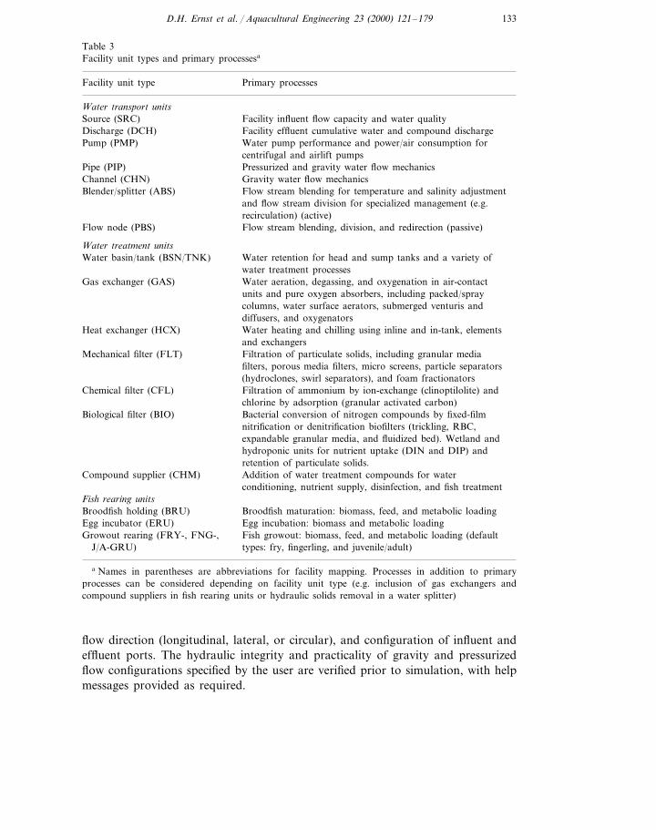
Table 3Facility unit types and primary processesa
Primary processesFacility unit type
Water transport unitsFacility influent flow capacity and water qualitySource (SRC)
Discharge (DCH) Facility effluent cumulative water and compound dischargeWater pump performance and power/air consumption forPump (PMP)centrifugal and airlift pumpsPressurized and gravity water flow mechanicsPipe (PIP)Gravity water flow mechanicsChannel (CHN)
Blender/splitter (ABS) Flow stream blending for temperature and salinity adjustmentand flow stream division for specialized management (e.g.recirculation) (active)Flow stream blending, division, and redirection (passive)Flow node (PBS)
Water treatment unitsWater basin/tank (BSN/TNK) Water retention for head and sump tanks and a variety of
water treatment processesGas exchanger (GAS) Water aeration, degassing, and oxygenation in air-contact
units and pure oxygen absorbers, including packed/spraycolumns, water surface aerators, submerged venturis anddiffusers, and oxygenators
Heat exchanger (HCX) Water heating and chilling using inline and in-tank, elementsand exchangers
Mechanical filter (FLT) Filtration of particulate solids, including granular mediafilters, porous media filters, micro screens, particle separators(hydroclones, swirl separators), and foam fractionators
Chemical filter (CFL) Filtration of ammonium by ion-exchange (clinoptilolite) andchlorine by adsorption (granular activated carbon)
Biological filter (BIO) Bacterial conversion of nitrogen compounds by fixed-filmnitrification or denitrification biofilters (trickling, RBC,expandable granular media, and fluidized bed). Wetland andhydroponic units for nutrient uptake (DIN and DIP) andretention of particulate solids.
Compound supplier (CHM) Addition of water treatment compounds for waterconditioning, nutrient supply, disinfection, and fish treatment
Fish rearing unitsBroodfish maturation: biomass, feed, and metabolic loadingBroodfish holding (BRU)
Egg incubator (ERU) Egg incubation: biomass and metabolic loadingGrowout rearing (FRY-, FNG-, Fish growout: biomass, feed, and metabolic loading (default
types: fry, fingerling, and juvenile/adult)J/A-GRU)
a Names in parentheses are abbreviations for facility mapping. Processes in addition to primaryprocesses can be considered depending on facility unit type (e.g. inclusion of gas exchangers andcompound suppliers in fish rearing units or hydraulic solids removal in a water splitter)
flow direction (longitudinal, lateral, or circular), and configuration of influent andeffluent ports. The hydraulic integrity and practicality of gravity and pressurizedflow configurations specified by the user are verified prior to simulation, with helpmessages provided as required.
134 D.H. Ernst et al. / Aquacultural Engineering 23 (2000) 121–179
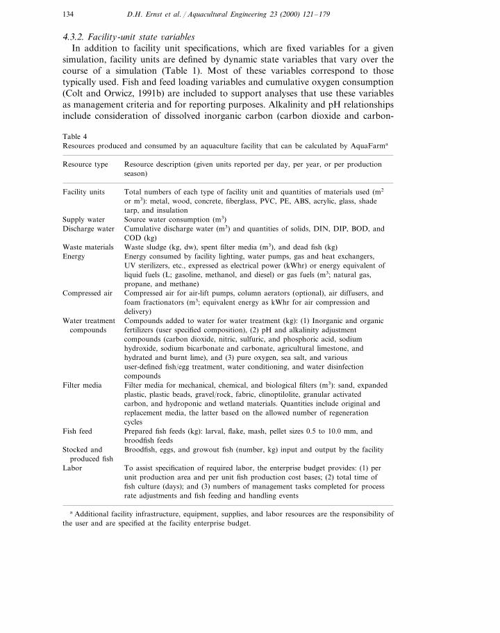
4.3.2. Facility-unit state 6ariablesIn addition to facility unit specifications, which are fixed variables for a given
simulation, facility units are defined by dynamic state variables that vary over thecourse of a simulation (Table 1). Most of these variables correspond to thosetypically used. Fish and feed loading variables and cumulative oxygen consumption(Colt and Orwicz, 1991b) are included to support analyses that use these variablesas management criteria and for reporting purposes. Alkalinity and pH relationshipsinclude consideration of dissolved inorganic carbon (carbon dioxide and carbon-
Table 4Resources produced and consumed by an aquaculture facility that can be calculated by AquaFarma
Resource type Resource description (given units reported per day, per year, or per productionseason)
Total numbers of each type of facility unit and quantities of materials used (m2Facility unitsor m3): metal, wood, concrete, fiberglass, PVC, PE, ABS, acrylic, glass, shadetarp, and insulation
Supply water Source water consumption (m3)Discharge water Cumulative discharge water (m3) and quantities of solids, DIN, DIP, BOD, and
COD (kg)Waste sludge (kg, dw), spent filter media (m3), and dead fish (kg)Waste materialsEnergy consumed by facility lighting, water pumps, gas and heat exchangers,EnergyUV sterilizers, etc., expressed as electrical power (kWhr) or energy equivalent ofliquid fuels (L; gasoline, methanol, and diesel) or gas fuels (m3; natural gas,propane, and methane)Compressed air for air-lift pumps, column aerators (optional), air diffusers, andCompressed airfoam fractionators (m3; equivalent energy as kWhr for air compression anddelivery)
Water treatment Compounds added to water for water treatment (kg): (1) Inorganic and organiccompounds fertilizers (user specified composition), (2) pH and alkalinity adjustment
compounds (carbon dioxide, nitric, sulfuric, and phosphoric acid, sodiumhydroxide, sodium bicarbonate and carbonate, agricultural limestone, andhydrated and burnt lime), and (3) pure oxygen, sea salt, and varioususer-defined fish/egg treatment, water conditioning, and water disinfectioncompoundsFilter media for mechanical, chemical, and biological filters (m3): sand, expandedFilter mediaplastic, plastic beads, gravel/rock, fabric, clinoptilolite, granular activatedcarbon, and hydroponic and wetland materials. Quantities include original andreplacement media, the latter based on the allowed number of regenerationcyclesPrepared fish feeds (kg): larval, flake, mash, pellet sizes 0.5 to 10.0 mm, andFish feedbroodfish feeds
Stocked and Broodfish, eggs, and growout fish (number, kg) input and output by the facilityproduced fish
To assist specification of required labor, the enterprise budget provides: (1) perLaborunit production area and per unit fish production cost bases; (2) total time offish culture (days); and (3) numbers of management tasks completed for processrate adjustments and fish feeding and handling events
a Additional facility infrastructure, equipment, supplies, and labor resources are the responsibility ofthe user and are specified at the facility enterprise budget.
135D.H. Ernst et al. / Aquacultural Engineering 23 (2000) 121–179
ates) and additional constituents of alkalinity (conjugate bases of dissociated acids).Constituents of dissolved inorganic nitrogen include ammonia, nitrite, and nitrate,and dissolved nitrogen gas can be considered. Dissolved inorganic phosphorous isconsidered equivalent to soluble reactive phosphorous (orthophosphate) and con-sists of ionization products of orthophosphoric acid (Boyd, 1990). For simplicity,other dissolved forms of phosphorous are not considered and inorganic phospho-rous applied as fertilizer is assumed to hydrolyze to the ortho form based on givenfertilizer solubilities. Nitrogen and phosphorous are variable constituents of organicparticulate solids, released in dissolved form when these solids are oxidized. Fishand water treatment chemicals are user-defined compounds that may be used for avariety of purposes, such as control of fish pathogens, water disinfectants andcompounds present in source waters (e.g. ozone and chlorine), and water condition-ing (e.g. dechlorination). Borate, silicate, and sulfate compounds can have minorimpacts on acid-base chemistry, especially for seawater systems, but can normallybe ignored.
Particulate solids are comprised of suspended and settleable, inorganic andorganic solids (expressed in terms of dry weight, dw; live phytoplankton notincluded). Suspended inorganic solids (clay turbidity) are considered in order toaccount for their impact on water clarity (expressed as Secchi disk visibility), whichis a function of total particulate solid and phytoplankton concentrations. Settleableinorganic and organic solids originate from various sources, e.g. in/organic fertiliz-ers, dead phytoplankton, uneaten feed, and fish fecal material. Settling rates andcarbon, nitrogen, and phosphorous contents of these solids depend on their sources.Settled solids originate from combined inorganic and organic settleable solids, andtheir composition varies in response to their sources.
4.3.3. Facility-unit processesPhysical, chemical, and biological mass-transfer processes and associated com-
pound sources and sinks that can occur in facility units are listed in Table 5. Inaddition, water flow mechanics and heat transfer are represented by energy transferprocesses. Methods used to model these mass and energy transfer processes (unitprocesses) are summarized in Appendix A. Unit processes can be individuallyselected for consideration, depending on user design objectives and analysis resolu-tion level. Unit processes can be passive, active, or both passive and active, and aresimulated accordingly. Examples of passive processes are water surface heat and gastransfer, bacterial processes, and primary productivity. Passive processes may beuncontrolled or indirectly controlled, e.g. primary productivity can be indirectlymanaged through the control of nutrient levels. Actively managed processes aredirectly controlled to maintain water quantity and quality variables at desiredlevels. Examples of active processes are water flow rate, heating, aeration, solidsfiltration, and compound addition. Air-water gas transfer of a fish pond is anexample of a combined passive-active process, in which aeration is used in responseto low oxygen levels but passive air-water gas transfer is also significant. Generally,in the context of this discussion, passive processes are defined by model parametersand active processes are defined by facility specifications.
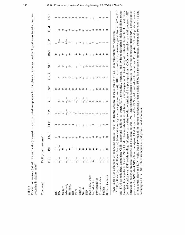
136 D.H. Ernst et al. / Aquacultural Engineering 23 (2000) 121–179
Tab
le5
Pre
senc
eof
sour
ces
(add
ed:
+)
and
sink
s(r
emov
ed:
−)
ofth
elis
ted
com
poun
dsfo
rth
eph
ysic
al,
chem
ical
,an
dbi
olog
ical
mas
str
ansf
erpr
oces
ses
occu
rrin
gin
faci
lity
unit
sa
Fac
ility
unit
proc
esse
sbC
ompo
und
FL
TC
HM
SOL
SST
OX
DN
ITD
NT
NP
PF
SMF
SCD
IFF
LO
CM
P
00
−0
−−
0+
−0
+/−
DO
+/−
+0
00
0+
0/−
00
DN
00
0+
/−+
/−0
0Sa
linit
y0
+/−
00
00
00
+0
0+
/−0
0−
++
/−+
/−+
+0
0A
lkal
init
y+
/−−
+/−
+/−
00
00
00
00
0+
0H
ardn
ess
+/−
+/−
+/−
0+
−+
−+
0+
/−+
0D
IC+
/−0
+−
0−
0+
TA
N0
−+
–+
/−N
itri
te+
/−+
/−0
0+
/−0
00
00
0−
0+
/−0
++
−−
0+
+/−
0N
itra
te−
+0
0+
/−+
/−0
+0
0−
+0
0+
−D
IP0
+/−
0−
−0
−+
+−
0+
−P
arti
cula
teso
lids
0+
−0
−0
00
Sett
led
solid
s−
00
00
00
00
Phy
topl
ankt
on0
+/−
+0
−0
0−
00
00
00
0−
0+
0−
Tre
atm
ent
chem
.+
/−−
0+
/−+
00
00
00
0−
00
Sulfi
de0
00
00
00
00
00
B,
Si,
S(s
ulfa
te)
0+
/−
aSe
eT
able
1fo
rde
finit
ions
ofco
mpo
und
nam
es.
Use
of‘0
’de
note
sab
senc
eof
mas
str
ansf
eror
lack
ofco
nsid
erat
ion
byA
quaF
arm
.b
FL
O,
influ
ent
(+)
and
efflu
ent
flow
(−)
(als
ow
ater
seep
age
and
prec
ipit
atio
n,se
ete
xt);
DIF
,pa
ssiv
ean
dac
tive
,ai
r-w
ater
gas
diff
usio
n(D
ICas
DC
and
TA
Nas
unio
nize
dam
mon
ia);
CM
P,
com
poun
dad
diti
onto
wat
er;
FL
T,
mec
hani
cal,
chem
ical
,an
dhy
drop
onic
/wet
land
biol
ogic
alfil
ters
(oth
erbi
olog
ical
filte
rsun
der
NIT
and
DN
T);
CH
M,
calc
ium
carb
onat
edi
ssol
utio
n(+
)an
dpr
ecip
itat
ion
(−)
and
deca
yof
trea
tmen
tch
emic
als;
SOL
,so
ilre
leas
e(+
)an
dup
take
(−);
SST
,so
lids
sett
ling
(in/
orga
nic
part
icul
ate
solid
s;no
sett
ling
ofliv
eph
ytop
lank
ton)
;O
XD
,he
tero
trop
hic
bact
eria
lpr
oces
ses;
NIT
,ni
trifi
cati
onba
cter
ial
proc
esse
s(p
assi
vean
dbi
olog
ical
filte
rs);
DN
T,
deni
trifi
cati
onba
cter
ial
proc
esse
s(p
assi
vean
dbi
olog
ical
filte
rs);
NP
P,
phyt
opla
nkto
npr
oces
ses
for
NP
P\
0(i
fN
PPB
0,re
vers
esi
gns)
.A
lkal
init
yis
rem
oved
for
TA
Nup
take
and
adde
dfo
rni
trat
ean
dD
Nup
take
.D
Nus
ede
pend
son
pres
ence
ofbl
ue-g
reen
alga
ean
dD
INle
vels
.D
ead
phyt
opla
nkto
nbe
com
epa
rtic
ulat
eor
gani
cso
lids;
FSM
,fis
hm
etab
olic
proc
esse
s,co
mpo
und
excr
etio
n(+
)an
dco
nsum
ptio
n(−
);F
SC,
fish
cons
umpt
ion
ofen
doge
nous
food
reso
urce
s.

137D.H. Ernst et al. / Aquacultural Engineering 23 (2000) 121–179
In addition to compounds, the water volume contained by a facility unit issubject to mass transfer, including influent and effluent flow, seepage infiltrationand loss, precipitation and runoff, and evaporation. Compound transfer via watertransfer are based on the assumptions that seepage water constituents are compara-ble to the bulk water volume, precipitation water is pure other than dissolved gases,and evaporation water has no constituents. Settled solids accumulate as a functionof contributing particulate solids and settling rates, their lack of disturbance(scouring), and incomplete bacterial oxidation. The accumulation of settled solidscan remove significant quantities of nutrients and oxygen demand and provide localanaerobic conditions that support denitrification. Settled solids can be removed byperiodic manual procedures (e.g. rearing unit vacuuming and filter cleaning) orcontinuous hydraulic procedures (e.g. dual-drain effluent configurations).
Facility unit differential equations are based on completely mixed hydraulics(James, 1984a; Tchobanoglous and Schroeder, 1985). While plug-flow hydraulicscharacterize certain types of facility units, e.g. raceway fish rearing units, thenecessity to consider plug-flow hydraulics with respect to overall simulation accu-racy is currently being assessed. When water stratification is considered, a facilityunit is modeled as two horizontal water layers of equal depth, and process rates andstate variables associated with each layer are maintained separately. Each of theselayers is completely mixed internally, and layers inter-mix at a rate dependent onenvironmental conditions. Possible stratified processes include physical processes(e.g. surface heat and gas transfer), chemical processes (e.g. pond soils), andbiological processes (e.g. primary productivity and settled solid oxidation). Possiblestratified water quality variables include temperature, dissolved gases, pH andalkalinity, nitrogen and phosphorous compounds, and organic particulate solids.For simplification, phytoplankton are assumed to maintain a homogenous distribu-tion over the water column.
4.3.4. Water transport unitsWater transport units are used to contain, blend, divide, and control water flow
streams (Table 3). Water transport units are installed as necessary to adequatelyrepresent water transport systems and determine flow rate capacity limits and pumppower requirements. To simplify facility construction, pipe fittings (e.g. elbows,tees, and valves) and short lengths of pipes and channels can be ignored. For clarityin facility mapping, however, water flow nodes can be used to represent all pointsof blending, division, and redirection of water flow streams by pipe fittings andchannel junctions. Any facility unit can have multiple influent and effluent flowstreams. Minor head losses of pipefittings are calculated as a proportion of themajor head losses of associated pipe lengths. Flow control devices for pipes andchannels are assumed to exist, but they are not explicitly defined. Specialized waterblenders and splitters are used for designated purposes, such as water flow blendingfor temperature and salinity adjustment and water flow division to achieve desiredwater recirculation rates.
138 D.H. Ernst et al. / Aquacultural Engineering 23 (2000) 121–179
4.3.5. Water treatment unitsWater treatment units are used to add, remove, and convert water borne
compounds and adjust water temperature (Table 3). Water treatment units typicallyspecialize in a particular unit process, but processes can be combined with a singlefacility unit as desired. Water treatment processes are primarily defined by theirgiven efficiencies or control levels. Specifications include set-point levels, set-pointtolerances, efficiencies of energy and material transfer, minimum and maximumallowed process rates, and process control methods.
Process efficiency is the primary control variable for filtration processes thatremove compounds from the water. For mechanical and chemical filters, processefficiency is specified as percent removal of the given compound per pass of waterthrough the filter. For biological filters, process efficiency is specified as kineticparameters of bacterial processes. For all filters, periodic requirements for mediacleaning (removal of accumulated solids) or regeneration (e.g. clinoptilolite andgranular activated carbon) over the course of a simulation can be accomplishedmanually by the facility manager or automatically by the facility unit.
Set-point level is the primary control variable for processes that add compoundsto the water and for temperature adjustment, for which the units used to expressset-point levels are those of the controlled variable. Pond fertilization is managedwith respect to set points for DIC, DIN, and/or DIP. For each process, constantrate, simple on/off, and proportional (throttled) process control methods can beused, the latter providing process rates that vary continuously or in discrete stepsover their given operational ranges. Integral-derivative process control can becombined with proportional control so that the rate of change and projected futurelevel of the controlled variable are considered in rate adjustments. Proportional andintegral-derivative controls are used to minimize oscillation of the controlledvariable around its set-point level (Heisler, 1984). Process control can be accom-plished manually by the facility manager or automatically by the facility unit. Forsome conditions, for example when both heaters and chillers are present, thecontrolled variable can be both decreased and increased to achieve a given setpoint. More typically, controlled variables can only be decreased or increased, forexample the addition of a compound to achieve a desired concentration. Set-pointtolerances and minimum and maximum allowed process rates are normally requiredfor realistic simulations, for example diurnal control of fish pond aerators inresponse to dissolved oxygen.
4.3.6. Fish rearing unitsFish rearing units can be designated for particular fish stocks (species), fish life
stages (broodfish, eggs, and growout fish), and fish size stages (e.g. fry, fingerling,and juvenile/adult) (Table 3). This supports movement of fish lots within the facilitybased on fish size and management of multiple life stage, multi-species, andpolyculture facilities. Fish rearing units can include most water treatment processes,e.g. fertilization, liming, and aeration for pond based aquaculture, and can utilizeprocess control methods as described for water treatment units.
139D.H. Ernst et al. / Aquacultural Engineering 23 (2000) 121–179
4.4. Fish stocks, populations, and lots
Production fish are represented at three levels of organization: fish stocks, fishpopulations, and fish lots. A fish stock consists of one or more fish populations,and a fish population is divided into one or more fish lots. A fish stock is a fishspecies or genetically distinct stock of fish, identified by common and scientificnames and defined by a set of biological performance parameters. Parameter valuesare provided for major aquaculture species and can be added for additionalaquaculture species. Fish populations provide a level of organization for themanagement and reporting tasks of related, cohort fish lots. Fish populations areuniquely identified by their origin fish stock, life stage (broodfish, egg, or growout),and production year. Broodfish, egg, and growout fish populations from the samefish stock are linked by life stage transfers, i.e. from broodfish spawning to eggstocking and from egg hatching to larvae/fry stocking.
Fish lots are fish management units within a fish population. Fish lots are definedby their current location (rearing unit), population size, and development state. Thelatter consists of accumulated temperature units (ATU) and photoperiod units(APU) for broodfish lots, accumulated temperature units for egg lots, and fish bodyweights for growout fish lots. At a point in time, fish lot states are maintained asmean values and fish weights within a growout fish lot can be represented as weightdistributions (histograms). Variability in fish weights within a growout fish lot canbe due to variability present at facility input, fish lot division and combining, andvariability in fish growth rates due to competition for limited food resources. Targetvalues for fish lot numbers and states are specified as production objectives or, inthe case of broodfish and egg target states, represent biological requirements. Initialvalues for these variables can be user specified, result from life stage transfers, orresult from fish stocking conditions that are required to achieve fish productionobjectives. Intermediate fish lot numbers and states are predicted by simulation.Methods used to model fish survival, development and growth, feeding, andmetabolism are summarized in Appendix A, under the fish biologist domain expert.
4.5. Facility managers
The facility managers are the physical plant manager and the fish culturemanager. Facility managers are assigned: (1) responsibilities and variables to bemonitored; (2) criteria for evaluation of monitored variables; and (3) allowedresponses to correct problems. Facility managers utilize domain experts for adjust-ing process rates and solving management problems. A management task can befully, partially, or not successful, depending on the availability of required facilityresources. The number of possible management responsibilities and responsesincreases with analysis resolution and facility complexity. Facility managers per-form their tasks at a given management time step, so that the desired managementintensity is emulated. Facility managers report problems and responses to manage-ment logs.
140 D.H. Ernst et al. / Aquacultural Engineering 23 (2000) 121–179
4.5.1. Physical plant managerActively managed mass and energy transfer processes of facility units are
controlled by the physical plant manager to maintain water quantity and qualityvariables at desired levels, including water flow, heat and gas transfer, andcompound conversion, addition, and removal. Based on facility specifications,active process rates can be adjusted: (1) manually, to emulate manual tasks of thephysical plant manager (e.g. manual on-demand aeration); or (2) automatically, toemulate automated process control (e.g. automated on-demand aeration). Manualmanagement tasks are simulated at the management time step, and automatedmanagement tasks are simulated at the simulation time step. For aquaculturefacilities, water flow rates are based on demands at fish rearing units, as determinedby the fish culture manager. For non-aquaculture facilities, water flow rates arecontrolled at water sources, to give constant or varying water flow rates. Water flowrates can be constrained by source water capacities and by water flow mechanicsand hydraulic loading constraints of facility units. Water management schemesinclude: (1) static water management with loss makeup to maintain minimumvolumes; (2) water flow-through with optional serial reuse; and (3) water recircula-tion at specified water recirculation and makeup rates.
4.5.2. Fish culture manager — production objecti6esThe fish culture manager is responsible for maintaining fish environmental
criteria and satisfying fish production objectives. This is accomplished through thecontrol of water flow and treatment processes, fish feeding rates, and fish biomassmanagement. These tasks are performed according to assigned management respon-sibilities, fish handling and biomass loading management strategies, and availablefacility resources. Fish production objectives are not achieved if they exceed fishperformance capacity or required facility resources are not available.
Fish production objectives are specified as: (1) calendar dates; (2) fish populationnumbers; and (3) fish development states (broodfish and eggs) or weights (growoutfish) at initial fish stocking and target transfer events. Fish transfer events includefish input to the facility, fish life stage transfers within the facility, and fishrelease/harvest from the facility. Alternatively, fish stocking specifications can bedetermined by AquaFarm such that target objectives are achieved. Productionobjectives are specified as combined quantities for fish populations and are dividedinto component values for fish lots. Fish lots within a fish population can bemanaged in a uniform manner or individually specified for temporal staging of fishproduction. Fish management size stages can be specified for growout lots to allowassignment of designated rearing units (e.g. fry, fingerling, and on-growing) andtypes of fish feed (pellet size and composition) based on fish size.
4.5.3. Fish culture manager–en6ironmental criteriaEnvironmental conditions are monitored at each management time step and
evaluated in relation to management criteria. Variables that can be responded toinclude water exchange rate and velocity, fish biomass density and loading rate,feed loading rate, cumulative oxygen consumption, dissolved oxygen saturation,
141D.H. Ernst et al. / Aquacultural Engineering 23 (2000) 121–179
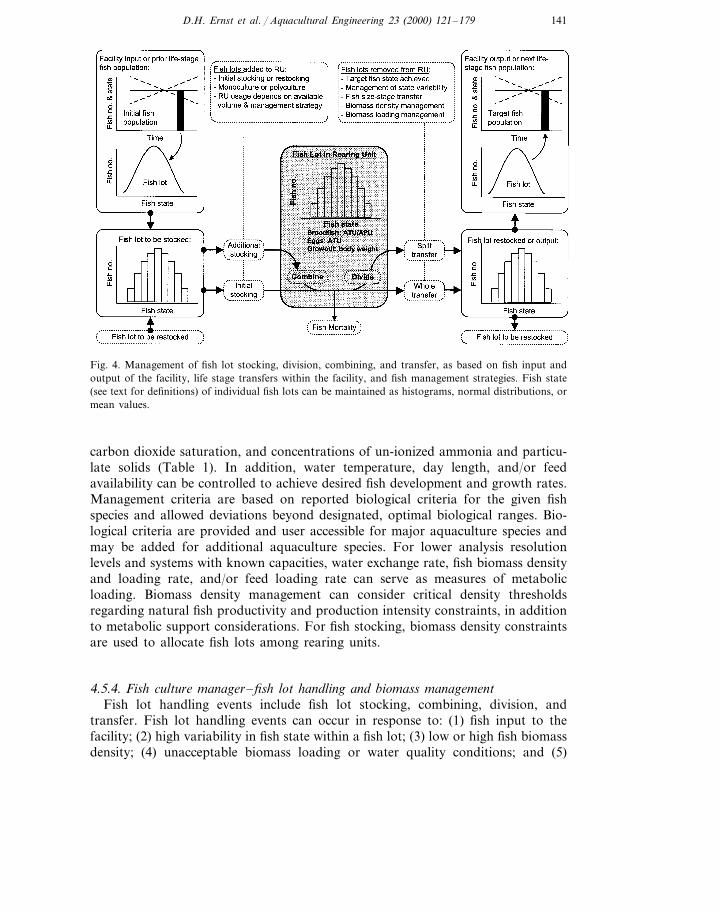
Fig. 4. Management of fish lot stocking, division, combining, and transfer, as based on fish input andoutput of the facility, life stage transfers within the facility, and fish management strategies. Fish state(see text for definitions) of individual fish lots can be maintained as histograms, normal distributions, ormean values.
carbon dioxide saturation, and concentrations of un-ionized ammonia and particu-late solids (Table 1). In addition, water temperature, day length, and/or feedavailability can be controlled to achieve desired fish development and growth rates.Management criteria are based on reported biological criteria for the given fishspecies and allowed deviations beyond designated, optimal biological ranges. Bio-logical criteria are provided and user accessible for major aquaculture species andmay be added for additional aquaculture species. For lower analysis resolutionlevels and systems with known capacities, water exchange rate, fish biomass densityand loading rate, and/or feed loading rate can serve as measures of metabolicloading. Biomass density management can consider critical density thresholdsregarding natural fish productivity and production intensity constraints, in additionto metabolic support considerations. For fish stocking, biomass density constraintsare used to allocate fish lots among rearing units.
4.5.4. Fish culture manager–fish lot handling and biomass managementFish lot handling events include fish lot stocking, combining, division, and
transfer. Fish lot handling events can occur in response to: (1) fish input to thefacility; (2) high variability in fish state within a fish lot; (3) low or high fish biomassdensity; (4) unacceptable biomass loading or water quality conditions; and (5)
142 D.H. Ernst et al. / Aquacultural Engineering 23 (2000) 121–179
achievement of threshold fish size stages, life stage transfers, and release or harvesttarget fish states (Fig. 4). Fish handling and biomass management responsibilitiesare defined by the following options.1. The use of rearing units is prioritized such that minimum overall fish densities
are maintained and either (a) fish lots are never combined or (b) lots arecombined only as required to stock all lots. Alternatively, the use of rearingunits is prioritized such that maximum overall fish densities are maintainedand either (c) lots are combined as required to stock all lots or (d) lots arecombined whenever possible to minimize use of rearing units and maximizefish densities.
2. If a facility holds multiple fish stocks, then either (a) different stocks aremaintained in separate rearing units (multi-species facilities) or (b) designatedstocks are combined within rearing units (polyculture facilities).
3. Fish lots are divided at stocking events to multiple rearing units as required byfish density constraints (yes/no). During culture, fish lots are transferred tosmaller rearing units if fish densities are too low (yes/no), and/or fish lots aretransferred whole or divided to larger rearing units if fish density is too high(yes/no).
4. Based on specified fish biomass loading and water quality criteria, (a) rearingunit water flow rates are adjusted and/or (b) fish lots are transferred whole ordivided to additional rearing units (adjustment of active process rates of fishrearing units is based directly on given set-point levels).
5. Growout fish lots are graded and divided during culture to reduce excessivevariability in fish weight (yes/no) and/or remove culls (yes/no). Growout fishlots are high graded and divided at transfer events to leave low grades forfurther culture (yes/no) and/or remove culls (yes/no).
4.5.5. Fish culture manager–management intensity and riskManagement intensity and risk levels are established through multiple specifica-
tions, including the type of facility, fish production objectives, fish lot handlingstrategies, fish biomass loading relative to maximum capacities, and degree ofproduction staging and maximization of cumulative production. Based on thesespecifications, management intensity can range from simple batch stocking andharvest practices to staged, continuous culture, high grade harvesting and restock-ing practices (Watten, 1992; Summerfelt et al., 1993). Management intensity is alsodefined by the size of the management time step, allowed variability in growout fishweights, minimum adjustment increments of process rates, and allowed tolerancesfor environmental variables to exceed optimal biological ranges. Management riskis quantified as a failure response time (FRT, hours) for fish rearing units. FRT isthe predicted time between failure of biomass support processes (e.g. water flow orin-pond aeration) and occurrence of fish mortality. Management risk is controlledby establishing a minimum allowed FRT for the facility. If rearing unit FRT valuesfall below this minimum, then fish biomass density is reduced, using the given fishlot handling rules.
143D.H. Ernst et al. / Aquacultural Engineering 23 (2000) 121–179
4.5.6. Fish culture manager–broodfish maturation and egg incubationBroodfish maturation is defined by accumulated temperature and/or photo-
period units. Spawning occurs when required levels of these units are achieved, asdefined by species-specific parameters maintained by the fish biologist. Watertemperature and day length can be controlled to achieve desired maturation ratesand spawning dates. Fish population number and spawning calculations accountfor female-male sex ratios, egg production per female, and fish spawning charac-teristics (i.e. once per year, repeat spawn, or death after spawning).
Egg development is defined by accumulated temperature units. Achievement ofdevelopment stages (eyed egg, hatched larvae, and first-feeding fry) is based ontemperature unit requirements of each stage, as defined by species-specificparameters maintained by the fish biologist. Egg handling can be restricted dur-ing sensitive development stages. Water temperature can be controlled to achievedesired development rates and first-feeding dates.
4.5.7. Fish culture manager — fish growoutFeeding strategies for fish growout can be based on: (1) endogenous (natural)
food resources only; (2) natural foods plus supplemental prepared feeds; or (3)prepared feeds only. Natural food resources can be managed indirectly by con-trol of fish densities and maintenance of nutrient levels for primary productivity.Prepared feeds are defined by their proximate composition and pellet size, andspecific feed types can be assigned to specific fish size stages. Prepared feeds areapplied as necessary to achieve target growth rates, based on initial and targetfish weights and dates and considering any contributions from natural foods. Fordaily simulations, prepared feed is applied once per day. For diurnal simulations,feed is applied according to the specified number of feedings per day and lengthof the daily feeding period, which can be specific to fish size stage. In addition,the impact of feed allocation strategies and application rates on food conversionefficiency and fish growth variability due to competition for limited food re-sources can be considered.
5. Facility and management simulation
5.1. Simulation processing
Following the establishment of facility and management specifications, facilityunits and fish lots are integrated and facility managers, fish populations, andresource units are updated over a series of time steps that total the simulationperiod. Facility components and managers are classified as simulation objectsat their highest level of hierarchical abstraction in the object oriented pro-gramming architecture. The simulation of these objects is administered by thesimulation manager. The simulation manager (1) maintains a simulation timeclock; (2) sends update commands to simulation objects based on their time
144 D.H. Ernst et al. / Aquacultural Engineering 23 (2000) 121–179
steps; and (3) for purposes of numerical integration, maintains arrays of statevariables and finite difference terms for the differential equations of facility unitsand fish lots. The simulation manager processes simulation objects in a genericmanner and has no need to be concerned with specific details of individualobjects, e.g. differential equations used to calculate difference terms or the man-agement protocols used by facility managers.
Manual procedures of the physical plant and fish culture managers are discon-tinuous, discrete events. Managers respond to update commands over a series ofmanagement time steps by reviewing their assigned responsibilities, responding asfacility resources allow, and logging management problems and completed tasksto management logs. In contrast, facility units and fish lots consist of continuousprocesses, represented by sets of simultaneous differential equations. Facilityunits and fish lots are simulated by solving state equations, updating statevariables, and logging state variable and process rate data over a series ofsimulation time steps. The state variables and equations used for facility unitsand fish lots depend on the analysis resolution level, fish performance methods,and passive and active unit processes under consideration. At each simulationstep, domain experts are used to calculate property, equilibrium, and processrate terms used in differential equations and management tasks.
5.2. Deterministic simulation
Simulations performed by AquaFarm are deterministic, in which identicalresults are predicted given the same set of input parameters and variable values,and all parameters and variables are expressed as mean values. Deterministicsimulations can be based on worst, best, and mean case scenarios, however,as controlled by the use of worst, best, and mean expected values for inputparameters and variables. Stochastic simulations are not currently supported byAquaFarm and their potential utility to AquaFarm users is under review.Stochastic simulations require multiple simulation runs (e.g. 30–100) to generateprobability distributions of predicted state variables, in which selected parametersand input variables vary stochastically within and between simulations (e.g.Griffin et al., 1981; Straskraba and Gnauck, 1985; Cuenco, 1989; Lu andPiedrahita, 1998). For aquaculture systems characterized by stochastic pro-cesses, the use of deterministic simulations represents a major analytical simplifi-cation. For example, solar-algae ponds are subject to stochastic climate variables(solar radiation, cloud cover, and wind speed) and similarly managed pondsoften show high variability between ponds in primary productivity and re-lated variables. However, the additional complexity of accomplishing and in-terpreting stochastic simulations is considerable and prolonged computer pro-cessing times are required. As in most aquacultural modeling studies, it isassumed that deterministic simulations are useful for facility design and shortand long term management decisions, even when significant stochastic behaviorexists.
145D.H. Ernst et al. / Aquacultural Engineering 23 (2000) 121–179
5.3. Numerical integration
Facility unit and fish lot differential equations can be solved by numerical oranalytical methods. Under numerical integration, differential equations are used asfinite difference equations to calculate finite difference terms (unit mass or energyper time). Related simulation objects are processed as a group, as determined by theexistence of shared variables and simultaneous processes. State variables and finitedifference terms of related simulation objects are collected into arrays at eachsimulation step and solved by the simulation manager using simultaneous, fourth-order Runge–Kutta integration (RK4; Elliot, 1984). RK4 integration is a powerfulnumerical integration method, capable of solving complex sets of simultaneousdifferential equations. However, RK4 integration may require small time steps, onthe order of minutes to hours, when high rates of energy or mass transfercharacterized by first-order kinetics exist in facility units (e.g. high rates of waterflow, active gas transfer, or fixed-film bacterial processes). In addition, RK4integration requires four iterations per time step for the calculation of differenceterms and update of state variables. Together, these requirements may result inexcessively long simulation execution times (e.g. 3 min, real time), depending on thenumber of simulation objects, length of the simulation period, and computerprocessing capacity.
5.4. Analytical integration
Analytical integration methods can accommodate high rate, first-order processesat large time steps (e.g. 1 day) and can be used to minimize required calculationsand simulation execution times. However, aquaculture facilities are typically char-acterized by simultaneous processes within and among facility units, and achieve-ment of analytical solutions normally requires the use of simplifying assumptions.To explore tradeoffs between mathematical rigor and simulation processing times,combined numerical-analytical and simplified analytical integration methods weredeveloped. For combined numerical-analytical integration, difference terms for eachof the four cycles of RK4 integration are calculated using analytical integration.For simplified analytical integration, differential equations are simplified to a levelwhere analytical solutions can be attained (Elliot, 1984). By this simplification,some simultaneous processes are unlinked, and thus simulation objects and thevariables they contain are updated in order of their increasing dependence on otherobjects and variables. The simulation order used is facility climate, up to downstream facility units, and finally fish lots. In addition, variables within a facility unitare updated in order of increasing dependence on other variables, beginning withwater temperature.
5.5. Management and simulation time steps
The size of the management time step is based on the desired managementintensity, i.e. the time interval between successive, periodic tasks of the facility and
146 D.H. Ernst et al. / Aquacultural Engineering 23 (2000) 121–179
fish culture managers. The size of the simulation time step is based on the natureof the aquaculture system and temporal resolution required to adequately capturesystem dynamics. Daily simulations (e.g. 1-day time step), for which diurnalvariables and processes are expressed and used as daily means, always representsome level of simplification at a degree depending on the type of facility andanalysis resolution level. For example, all fish culture systems are at least character-ized by diurnal fish process, resulting from day-versus-night activity levels andfeeding rates of fish. However, diurnal simulations (e.g. 1-h time step) are requiredonly when the variability of process rates and state variables within a day period,and associated management responses, must be considered to adequately representthe system. For example, diurnal simulations may be used for solar-algae ponds forhigh-resolution modeling of heat transfer and primary productivity, and they maybe used for intensive systems for high-resolution modeling of fish feeding andmetabolism. Any consideration of process management within a 24-h periodrequires diurnal simulations, e.g. pre-dawn aeration for pond-based systems ordiurnal control of oxygen injection rates for intensive systems. For RK4 integra-tion, daily simulations may require time steps of less than one day, but variablesand processes are still used as daily means.
6. AquaFarm testing, calibration, and validation
The program code modules comprising AquaFarm were tested, debugged, andverified to perform according to the previously reported or newly developedmethods from which they were developed. Testing alone was sufficient to validatedata input and output, management, and display tasks, integration procedures fordifferential equations, and simulation of facility management. Similarly, the validityof actively managed processes was largely dependent on given process specifications(e.g. water treatment efficiencies) and confirmed by direct testing. Finally, Aqua-Farm was verified to provide full ranges of expected results (dependent variables)for all types of extensive and intensive aquaculture systems, solely by adjustment ofinput parameters and independent variables over their reasonable ranges. In sum,this testing verified the internal and external consistency of AquaFarm (Cuenco,1989) and indicated sufficient development of the collected parameters, variables,and unit processes considered and their combined expression as differential equa-tions and integrated functions.
Requirements for calibration and validation of the component models (Cuenco,1989) used in AquaFarm was variable, depending on the nature of these modelsand their level of development in the supporting literature. Calibration is theprocess of determining values for model parameters (equation coefficients andexponents) through regression procedures using empirical datasets. Due to the wideuse of mechanistic models in AquaFarm, most parameters have inherent meaningwith respect to the processes they represent and can be directly estimated usingreported values. Validation is the process of testing how much confidence can beplaced on simulation results. Calibration and validation accomplishments to date
147D.H. Ernst et al. / Aquacultural Engineering 23 (2000) 121–179
are given in Appendix A. For some component models, these accomplishments arepreliminary and/or rely on parameter values from the supporting literature. Com-pletion of calibration and validation procedures for selected, unit process models isongoing, as described in the conclusion to this paper.
7. AquaFarm application
Application of AquaFarm to various aquaculture systems and analyses is demon-strated in the following examples. For each exercise, site-specific facility variables,management strategies, and model parameters were entered into AquaFarm. Addi-tional parameters of unit process models were based on default values provided byAquaFarm. Simulations were then performed to generate fish culture schedules,chronologies of facility state variables and processes, and required resources toachieve fish production objectives. Finally, predicted performance data were com-pared to empirical data from representative studies in the literature.
Reporting of the specifications and results of these simulation exercises is limitedto overviews, with a focus on core issues of fish performance and dominant facilityprocesses. The specifications and results presented are not necessarily meant torepresent critical variables, but rather to illustrate the range of detail and analyticalcapacities available in AquaFarm. The design procedure presented earlier is notdemonstrated, rather the results of a single simulation are presented for each systemtype. Enterprise budgets are not presented, for which unit costs are highly specificto location and budget formats have already been described. While not shown,however, any of these examples could use a series of simulations to considerresource use, management intensity, and budgetary requirements over a range offish production levels and alternative design and management strategies.
For all of these exercises, it is emphasized that the accuracy of simulation resultsrelative to empirically determined results was highly dependent on the accuracy ofsite-specific variables and parameters. When simulation results are said to be‘comparable’ to the referenced studies, it is meant that simulation results werewithin the range of reported results and showed similar cause-and-effect behaviorfor independent and dependent variables. Conclusions for these exercises includethe caveat that fully comprehensive reporting of methods and results were notavailable in the studies used, as is typical in technical papers, requiring theestimation of some design and management variables.
In these simulation exercises, results showed close agreement between simplifiedanalytical integration and rigorous numerical (RK4) integration for a variety ofsystem types, using time steps of 1 day for daily simulations and 1 h for diurnalsimulations. For daily simulations especially, in which state variables (as dailymeans) normally change relatively slowly over time, simplifications used to uncou-ple simultaneous processes so that analytical solutions could be achieved wereclearly supported. Combined analytical-numerical integration was successful inachieving considerably larger time steps than allowed by purely numericalintegration.
148 D.H. Ernst et al. / Aquacultural Engineering 23 (2000) 121–179
7.1. Tilapia production in ponds
AquaFarm was applied to the production of Nile tilapia (Oreochromis niloticus)in tropical (10° latitude) solar-algae ponds. Specifications and results of this exerciseare provided in Table 6 and Figs, 5, 6, and 7. Diurnal simulations were used andwater stratification was considered. Agriculture limestone (calcium carbonate) andfertilizer were applied to maintain DIC (in terms of alkalinity), DIN, and DIPnutrient levels for primary productivity. Fertilized ponds received lime and fertilizeronly. Fertilized-fed ponds received lime and fertilizer by the same managementcriteria as fertilized ponds, with additional application of pelletized feed as requiredto achieve target fish growth rates. Fertilizer consisted of combined chicken manureand ammonium nitrate, with the latter added to achieve a nitrogen-phosphorous ratioof 5.0, based on the manure nitrogen and phosphorous contents (Lin et al., 1997).
Predicted water quality regimes and fertilizer and feed requirements were com-parable to reported values for tilapia production under similar site and managementconditions. As expected, total lime application rates were in the low range of reportedrates (Boyd, 1990; Boyd and Bowman, 1997), for which pond source water had lowalkalinity but soils were assumed to already be neutralized with respect to exchangeacidity (base unsaturation). The nitrogen and phosphorous application rates usedwere within reported ranges for tilapia production in fertilized ponds, which range2.0–4.0 kg N ha−1 day−1 at N:P ratios that range 1:1–8:1 (Lin et al., 1997). Forfertilized and fertilized-fed ponds, simulated fish growth rates and total productionper hectare, fish density level at the onset of feeding, and required feed applicationrates were comparable to reported results (Diana et al., 1996; Diana, 1997; Linet al., 1997). Fish production and application of fertilizer and feed were adequatelyestimated using a daily time step with no consideration of water stratification.However, as generally found for solar-algae ponds, diurnal simulations and con-sideration of stratification were required to estimate extremes in water qualityregimes. Typical diurnal profiles of temperature and dissolved oxygen, as shown inFig. 7 for mid summer, were comparable to reported profiles for stratified tropicalponds (Losordo and Piedrahita, 1991; Piedrahita et al., 1993; Culberson andPiedrahita, 1994). The maximum divergence in water quality between the top andbottom layers was controlled by the specified regime of daily-minimum layer mixingrates.
7.2. Catfish production in ponds
AquaFarm was applied to production of channel catfish (Ictaluras punctatus) intemperate (30° latitude) solar-algae ponds. Specifications and results of this exerciseare provided in Table 7 and Figs. 8, 9, and 10. Diurnal simulations were used andwater stratification was considered. Single fish stocking and harvest events were usedto simplify this example, rather than the periodic high-grade harvesting and partialre-stocking methods typically employed for catfish production. Target fish numbersand weights were specified such that feed application rate increased to a maximumof 110 kg ha−1 day−1, in order to emulate conditions used in Cole and Boyd
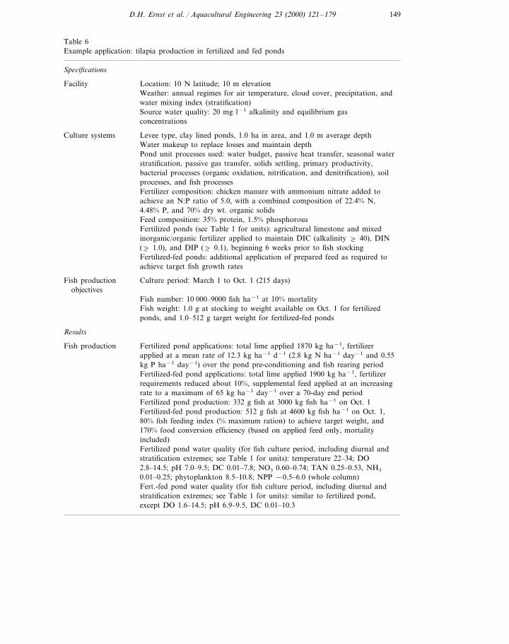
149D.H. Ernst et al. / Aquacultural Engineering 23 (2000) 121–179
Table 6Example application: tilapia production in fertilized and fed ponds
Specifications
Facility Location: 10 N latitude; 10 m elevationWeather: annual regimes for air temperature, cloud cover, precipitation, andwater mixing index (stratification)Source water quality: 20 mg l−1 alkalinity and equilibrium gasconcentrations
Levee type, clay lined ponds, 1.0 ha in area, and 1.0 m average depthCulture systemsWater makeup to replace losses and maintain depthPond unit processes used: water budget, passive heat transfer, seasonal waterstratification, passive gas transfer, solids settling, primary productivity,bacterial processes (organic oxidation, nitrification, and denitrification), soilprocesses, and fish processesFertilizer composition: chicken manure with ammonium nitrate added toachieve an N:P ratio of 5.0, with a combined composition of 22.4% N,4.48% P, and 70% dry wt. organic solidsFeed composition: 35% protein, 1.5% phosphorousFertilized ponds (see Table 1 for units): agricultural limestone and mixedinorganic/organic fertilizer applied to maintain DIC (alkalinity \6 40), DIN(\6 1.0), and DIP (\6 0.1), beginning 6 weeks prior to fish stockingFertilized-fed ponds: additional application of prepared feed as required toachieve target fish growth rates
Culture period: March 1 to Oct. 1 (215 days)Fish productionobjectives
Fish number: 10 000–9000 fish ha−1 at 10% mortalityFish weight: 1.0 g at stocking to weight available on Oct. 1 for fertilizedponds, and 1.0–512 g target weight for fertilized-fed ponds
Results
Fertilized pond applications: total lime applied 1870 kg ha−1, fertilizerFish productionapplied at a mean rate of 12.3 kg ha−1 d−1 (2.8 kg N ha−1 day−1 and 0.55kg P ha−1 day−1) over the pond pre-conditioning and fish rearing periodFertilized-fed pond applications: total lime applied 1900 kg ha−1, fertilizerrequirements reduced about 10%, supplemental feed applied at an increasingrate to a maximum of 65 kg ha−1 day−1 over a 70-day end periodFertilized pond production: 332 g fish at 3000 kg fish ha−1 on Oct. 1Fertilized-fed pond production: 512 g fish at 4600 kg fish ha−1 on Oct. 1,80% fish feeding index (% maximum ration) to achieve target weight, and170% food conversion efficiency (based on applied feed only, mortalityincluded)Fertilized pond water quality (for fish culture period, including diurnal andstratification extremes; see Table 1 for units): temperature 22–34; DO2.8–14.5; pH 7.0–9.5; DC 0.01–7.8; NO3 0.60–0.74; TAN 0.25–0.53, NH3
0.01–0.25; phytoplankton 8.5–10.8; NPP −0.5–6.0 (whole column)Fert.-fed pond water quality (for fish culture period, including diurnal andstratification extremes; see Table 1 for units): similar to fertilized pond,except DO 1.6–14.5; pH 6.9–9.5, DC 0.01–10.3
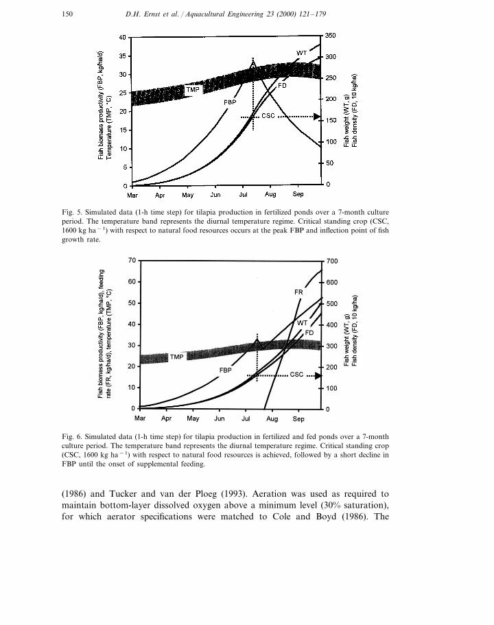
150 D.H. Ernst et al. / Aquacultural Engineering 23 (2000) 121–179
Fig. 5. Simulated data (1-h time step) for tilapia production in fertilized ponds over a 7-month cultureperiod. The temperature band represents the diurnal temperature regime. Critical standing crop (CSC,1600 kg ha−1) with respect to natural food resources occurs at the peak FBP and inflection point of fishgrowth rate.
Fig. 6. Simulated data (1-h time step) for tilapia production in fertilized and fed ponds over a 7-monthculture period. The temperature band represents the diurnal temperature regime. Critical standing crop(CSC, 1600 kg ha−1) with respect to natural food resources is achieved, followed by a short decline inFBP until the onset of supplemental feeding.
(1986) and Tucker and van der Ploeg (1993). Aeration was used as required tomaintain bottom-layer dissolved oxygen above a minimum level (30% saturation),for which aerator specifications were matched to Cole and Boyd (1986). The
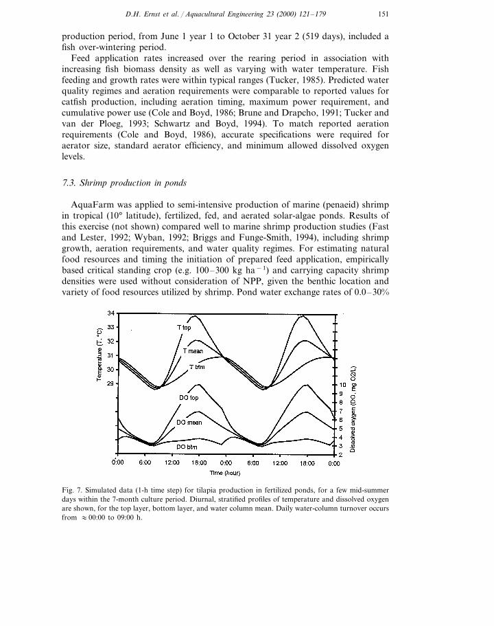
151D.H. Ernst et al. / Aquacultural Engineering 23 (2000) 121–179
production period, from June 1 year 1 to October 31 year 2 (519 days), included afish over-wintering period.
Feed application rates increased over the rearing period in association withincreasing fish biomass density as well as varying with water temperature. Fishfeeding and growth rates were within typical ranges (Tucker, 1985). Predicted waterquality regimes and aeration requirements were comparable to reported values forcatfish production, including aeration timing, maximum power requirement, andcumulative power use (Cole and Boyd, 1986; Brune and Drapcho, 1991; Tucker andvan der Ploeg, 1993; Schwartz and Boyd, 1994). To match reported aerationrequirements (Cole and Boyd, 1986), accurate specifications were required foraerator size, standard aerator efficiency, and minimum allowed dissolved oxygenlevels.
7.3. Shrimp production in ponds
AquaFarm was applied to semi-intensive production of marine (penaeid) shrimpin tropical (10° latitude), fertilized, fed, and aerated solar-algae ponds. Results ofthis exercise (not shown) compared well to marine shrimp production studies (Fastand Lester, 1992; Wyban, 1992; Briggs and Funge-Smith, 1994), including shrimpgrowth, aeration requirements, and water quality regimes. For estimating naturalfood resources and timing the initiation of prepared feed application, empiricallybased critical standing crop (e.g. 100–300 kg ha−1) and carrying capacity shrimpdensities were used without consideration of NPP, given the benthic location andvariety of food resources utilized by shrimp. Pond water exchange rates of 0.0–30%
Fig. 7. Simulated data (1-h time step) for tilapia production in fertilized ponds, for a few mid-summerdays within the 7-month culture period. Diurnal, stratified profiles of temperature and dissolved oxygenare shown, for the top layer, bottom layer, and water column mean. Daily water-column turnover occursfrom :00:00 to 09:00 h.
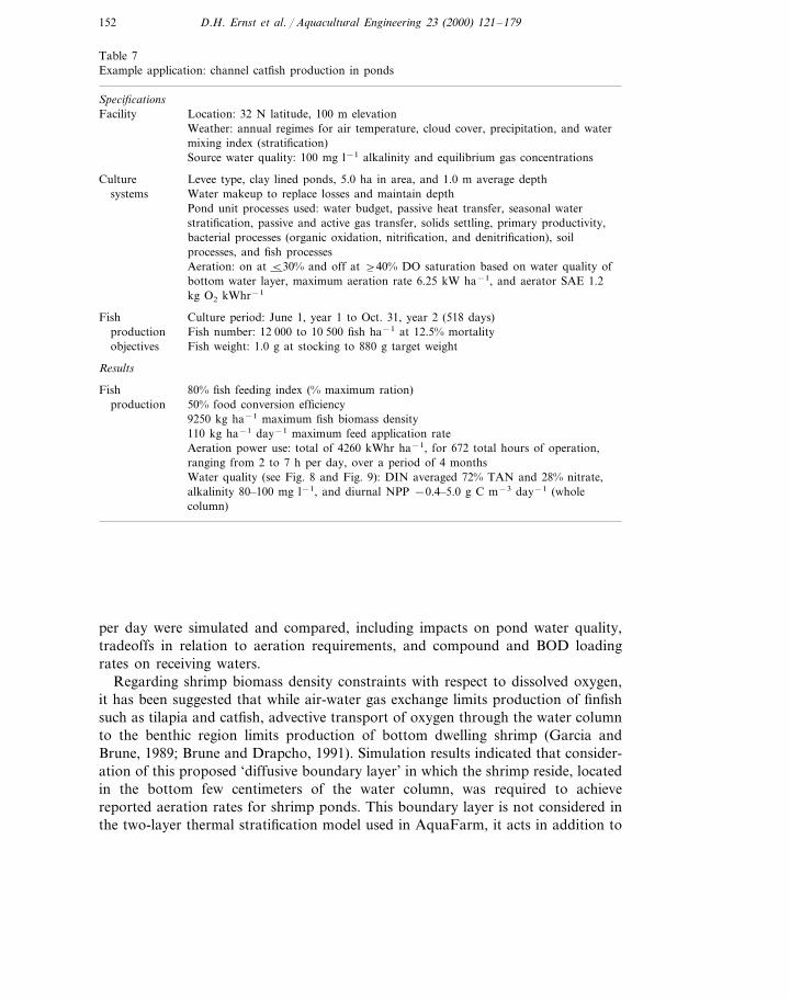
152 D.H. Ernst et al. / Aquacultural Engineering 23 (2000) 121–179
Table 7Example application: channel catfish production in ponds
SpecificationsLocation: 32 N latitude, 100 m elevationFacilityWeather: annual regimes for air temperature, cloud cover, precipitation, and watermixing index (stratification)Source water quality: 100 mg l−1 alkalinity and equilibrium gas concentrations
Culture Levee type, clay lined ponds, 5.0 ha in area, and 1.0 m average depthWater makeup to replace losses and maintain depthsystemsPond unit processes used: water budget, passive heat transfer, seasonal waterstratification, passive and active gas transfer, solids settling, primary productivity,bacterial processes (organic oxidation, nitrification, and denitrification), soilprocesses, and fish processesAeration: on at B30% and off at \6 40% DO saturation based on water quality ofbottom water layer, maximum aeration rate 6.25 kW ha−1, and aerator SAE 1.2kg O2 kWhr−1
Fish Culture period: June 1, year 1 to Oct. 31, year 2 (518 days)production Fish number: 12 000 to 10 500 fish ha−1 at 12.5% mortality
Fish weight: 1.0 g at stocking to 880 g target weightobjectives
Results
80% fish feeding index (% maximum ration)Fishproduction 50% food conversion efficiency
9250 kg ha−1 maximum fish biomass density110 kg ha−1 day−1 maximum feed application rateAeration power use: total of 4260 kWhr ha−1, for 672 total hours of operation,ranging from 2 to 7 h per day, over a period of 4 monthsWater quality (see Fig. 8 and Fig. 9): DIN averaged 72% TAN and 28% nitrate,alkalinity 80–100 mg l−1, and diurnal NPP −0.4–5.0 g C m−3 day−1 (wholecolumn)
per day were simulated and compared, including impacts on pond water quality,tradeoffs in relation to aeration requirements, and compound and BOD loadingrates on receiving waters.
Regarding shrimp biomass density constraints with respect to dissolved oxygen,it has been suggested that while air-water gas exchange limits production of finfishsuch as tilapia and catfish, advective transport of oxygen through the water columnto the benthic region limits production of bottom dwelling shrimp (Garcia andBrune, 1989; Brune and Drapcho, 1991). Simulation results indicated that consider-ation of this proposed ‘diffusive boundary layer’ in which the shrimp reside, locatedin the bottom few centimeters of the water column, was required to achievereported aeration rates for shrimp ponds. This boundary layer is not considered inthe two-layer thermal stratification model used in AquaFarm, it acts in addition to
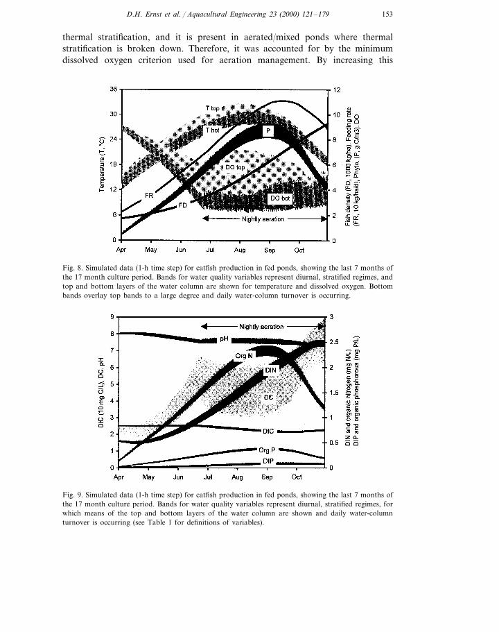
153D.H. Ernst et al. / Aquacultural Engineering 23 (2000) 121–179
thermal stratification, and it is present in aerated/mixed ponds where thermalstratification is broken down. Therefore, it was accounted for by the minimumdissolved oxygen criterion used for aeration management. By increasing this
Fig. 8. Simulated data (1-h time step) for catfish production in fed ponds, showing the last 7 months ofthe 17 month culture period. Bands for water quality variables represent diurnal, stratified regimes, andtop and bottom layers of the water column are shown for temperature and dissolved oxygen. Bottombands overlay top bands to a large degree and daily water-column turnover is occurring.
Fig. 9. Simulated data (1-h time step) for catfish production in fed ponds, showing the last 7 months ofthe 17 month culture period. Bands for water quality variables represent diurnal, stratified regimes, forwhich means of the top and bottom layers of the water column are shown and daily water-columnturnover is occurring (see Table 1 for definitions of variables).
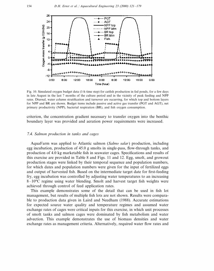
154 D.H. Ernst et al. / Aquacultural Engineering 23 (2000) 121–179
Fig. 10. Simulated oxygen budget data (1-h time step) for catfish production in fed ponds, for a few daysin late August in the last 7 months of the culture period and in the vicinity of peak feeding and NPPrates. Diurnal, water column stratification and turnover are occurring, for which top and bottom layersfor NPP and BR are shown. Budget items include passive and active gas transfer (PGT and AGT), netprimary productivity (NPP), bacterial respiration (BR), and fish oxygen consumption.
criterion, the concentration gradient necessary to transfer oxygen into the benthicboundary layer was provided and aeration power requirements were increased.
7.4. Salmon production in tanks and cages
AquaFarm was applied to Atlantic salmon (Salmo salar) production, includingegg incubation, production of 45.0 g smolts in single-pass, flow-through tanks, andproduction of 4.0 kg marketable fish in seawater cages. Specifications and results ofthis exercise are provided in Table 8 and Figs. 11 and 12. Egg, smolt, and growoutproduction stages were linked by their temporal sequence and population numbers,for which dates and population numbers were given for the input of fertilized eggsand output of harvested fish. Based on the intermediate target date for first-feedingfry, egg incubation was controlled by adjusting water temperatures to an increasing8–10°C regime using water blending. Smolt and harvest target fish weights wereachieved through control of feed application rates.
This example demonstrates some of the detail that can be used in fish lotmanagement, but results of multiple fish lots are not shown. Results were compara-ble to production data given in Laird and Needham (1988). Accurate estimationsfor expected source water quality and temperature regimes and assumed waterexchange rates of cages were critical inputs for this exercise, in which unit processesof smolt tanks and salmon cages were dominated by fish metabolism and wateradvection. This example demonstrates the use of biomass densities and waterexchange rates as management criteria. Alternatively, required water flow rates and
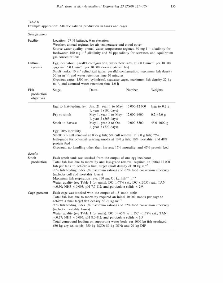
155D.H. Ernst et al. / Aquacultural Engineering 23 (2000) 121–179
Table 8Example application: Atlantic salmon production in tanks and cages
Specifications
Facility Location: 57 N latitude, 0 m elevationWeather: annual regimes for air temperature and cloud coverSource water quality: annual water temperature regimes, 50 mg l−1 alkalinity forfreshwater, 100 mg l−1 alkalinity and 35 ppt salinity for seawater, and equilibriumgas concentrations
Culture Egg incubators: parallel configuration, water flow rates at 2.0 l min−1 per 10 000eggs and 5.0 l min−1 per 10 000 alevin (hatched fry)systemsSmolt tanks: 10 m3 cylindrical tanks, parallel configuration, maximum fish density30 kg m−3, and water retention time 30 minutesGrowout cages: 1500 m3, cylindrical, seawater cages, maximum fish density 22 kgm−3, and assumed water retention time 1.0 h
Number WeightsStage DatesFishproductionobjectives
15 000–12 000 Egg to 0.2 gJan. 21, year 1 to MayEgg to first-feeding fry1, year 1 (100 days)
Fry to smolt 12 000–6600 0.2–45.0 gMay 1, year 1 to May1, year 2 (365 days)
45.0–4000 gMay 1, year 2 to Oct. 10 000–8500Smolt to harvest1, year 3 (520 days)
Egg: 20% mortalitySmolt: 5% cull removal at 0.75 g fish; 5% cull removal at 2.0 g fish; 75%high-grade for potential yearling smolts at 10.0 g fish; 10% mortality, and 48%protein feedGrowout: no handling other than harvest; 15% mortality, and 45% protein feed
ResultsEach smolt tank was stocked from the output of one egg incubatorSmolt
production Total fish loss due to mortality and low-grade removal required an initial 12 000fish per tank to achieve a final target smolt density of 30 kg m−3
70% fish feeding index (% maximum ration) and 67% food conversion efficiency(includes cull and mortality losses)Maximum fish respiration rate: 170 mg O2 kg fish−1 h−1
Water quality (see Table 1 for units): DO ]77% sat.; DC 5355% sat.; TAN50.30; NH3 50.003; pH 7.7–8.2; and particulate solids 52.9
Each cage was stocked with the output of 1.5 smolt tanksCage growoutTotal fish loss due to mortality required an initial 10 000 smolts per cage toachieve a final target fish density of 22 kg m−3
90% fish feeding index (% maximum ration) and 52% food conversion efficiency(includes mortality losses)Water quality (see Table 1 for units): DO \6 65% sat.; DC B178% sat.; TANB0.37; NH3 B0.005; pH 8.0–8.2; and particulate solids B3.5Total compound loading on supporting water body per 1000 kg fish produced:680 kg dry wt. solids; 750 kg BOD; 80 kg DIN; and 20 kg DIP
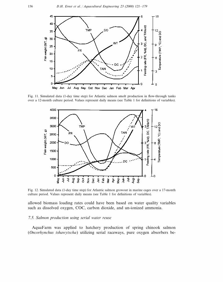
156 D.H. Ernst et al. / Aquacultural Engineering 23 (2000) 121–179
Fig. 11. Simulated data (1-day time step) for Atlantic salmon smolt production in flow-through tanksover a 12-month culture period. Values represent daily means (see Table 1 for definitions of variables).
Fig. 12. Simulated data (1-day time step) for Atlantic salmon growout in marine cages over a 17-monthculture period. Values represent daily means (see Table 1 for definitions of variables).
allowed biomass loading rates could have been based on water quality variablessuch as dissolved oxygen, COC, carbon dioxide, and un-ionized ammonia.
7.5. Salmon production using serial water reuse
AquaFarm was applied to hatchery production of spring chinook salmon(Oncorhynchus tshawytscha) utilizing serial raceways, pure oxygen absorbers be-
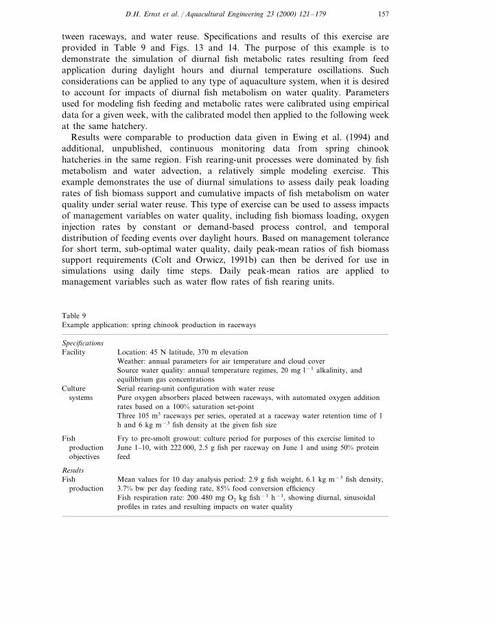
157D.H. Ernst et al. / Aquacultural Engineering 23 (2000) 121–179
tween raceways, and water reuse. Specifications and results of this exercise areprovided in Table 9 and Figs. 13 and 14. The purpose of this example is todemonstrate the simulation of diurnal fish metabolic rates resulting from feedapplication during daylight hours and diurnal temperature oscillations. Suchconsiderations can be applied to any type of aquaculture system, when it is desiredto account for impacts of diurnal fish metabolism on water quality. Parametersused for modeling fish feeding and metabolic rates were calibrated using empiricaldata for a given week, with the calibrated model then applied to the following weekat the same hatchery.
Results were comparable to production data given in Ewing et al. (1994) andadditional, unpublished, continuous monitoring data from spring chinookhatcheries in the same region. Fish rearing-unit processes were dominated by fishmetabolism and water advection, a relatively simple modeling exercise. Thisexample demonstrates the use of diurnal simulations to assess daily peak loadingrates of fish biomass support and cumulative impacts of fish metabolism on waterquality under serial water reuse. This type of exercise can be used to assess impactsof management variables on water quality, including fish biomass loading, oxygeninjection rates by constant or demand-based process control, and temporaldistribution of feeding events over daylight hours. Based on management tolerancefor short term, sub-optimal water quality, daily peak-mean ratios of fish biomasssupport requirements (Colt and Orwicz, 1991b) can then be derived for use insimulations using daily time steps. Daily peak-mean ratios are applied tomanagement variables such as water flow rates of fish rearing units.
Table 9Example application: spring chinook production in raceways
SpecificationsLocation: 45 N latitude, 370 m elevationFacilityWeather: annual parameters for air temperature and cloud coverSource water quality: annual temperature regimes, 20 mg l−1 alkalinity, andequilibrium gas concentrations
Culture Serial rearing-unit configuration with water reusesystems Pure oxygen absorbers placed between raceways, with automated oxygen addition
rates based on a 100% saturation set-pointThree 105 m3 raceways per series, operated at a raceway water retention time of 1h and 6 kg m−3 fish density at the given fish size
Fish Fry to pre-smolt growout: culture period for purposes of this exercise limited toproduction June 1–10, with 222 000, 2.5 g fish per raceway on June 1 and using 50% proteinobjectives feed
ResultsMean values for 10 day analysis period: 2.9 g fish weight, 6.1 kg m−3 fish density,Fish3.7% bw per day feeding rate, 85% food conversion efficiencyproductionFish respiration rate: 200–480 mg O2 kg fish−1 h−1, showing diurnal, sinusoidalprofiles in rates and resulting impacts on water quality
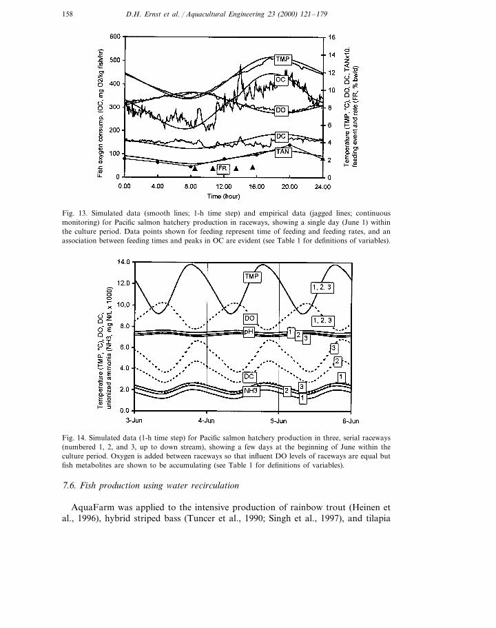
158 D.H. Ernst et al. / Aquacultural Engineering 23 (2000) 121–179
Fig. 13. Simulated data (smooth lines; 1-h time step) and empirical data (jagged lines; continuousmonitoring) for Pacific salmon hatchery production in raceways, showing a single day (June 1) withinthe culture period. Data points shown for feeding represent time of feeding and feeding rates, and anassociation between feeding times and peaks in OC are evident (see Table 1 for definitions of variables).
Fig. 14. Simulated data (1-h time step) for Pacific salmon hatchery production in three, serial raceways(numbered 1, 2, and 3, up to down stream), showing a few days at the beginning of June within theculture period. Oxygen is added between raceways so that influent DO levels of raceways are equal butfish metabolites are shown to be accumulating (see Table 1 for definitions of variables).
7.6. Fish production using water recirculation
AquaFarm was applied to the intensive production of rainbow trout (Heinen etal., 1996), hybrid striped bass (Tuncer et al., 1990; Singh et al., 1997), and tilapia
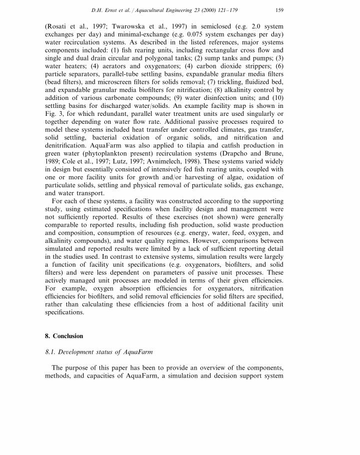
159D.H. Ernst et al. / Aquacultural Engineering 23 (2000) 121–179
(Rosati et al., 1997; Twarowska et al., 1997) in semiclosed (e.g. 2.0 systemexchanges per day) and minimal-exchange (e.g. 0.075 system exchanges per day)water recirculation systems. As described in the listed references, major systemscomponents included: (1) fish rearing units, including rectangular cross flow andsingle and dual drain circular and polygonal tanks; (2) sump tanks and pumps; (3)water heaters; (4) aerators and oxygenators; (4) carbon dioxide strippers; (6)particle separators, parallel-tube settling basins, expandable granular media filters(bead filters), and microscreen filters for solids removal; (7) trickling, fluidized bed,and expandable granular media biofilters for nitrification; (8) alkalinity control byaddition of various carbonate compounds; (9) water disinfection units; and (10)settling basins for discharged water/solids. An example facility map is shown inFig. 3, for which redundant, parallel water treatment units are used singularly ortogether depending on water flow rate. Additional passive processes required tomodel these systems included heat transfer under controlled climates, gas transfer,solid settling, bacterial oxidation of organic solids, and nitrification anddenitrification. AquaFarm was also applied to tilapia and catfish production ingreen water (phytoplankton present) recirculation systems (Drapcho and Brune,1989; Cole et al., 1997; Lutz, 1997; Avnimelech, 1998). These systems varied widelyin design but essentially consisted of intensively fed fish rearing units, coupled withone or more facility units for growth and/or harvesting of algae, oxidation ofparticulate solids, settling and physical removal of particulate solids, gas exchange,and water transport.
For each of these systems, a facility was constructed according to the supportingstudy, using estimated specifications when facility design and management werenot sufficiently reported. Results of these exercises (not shown) were generallycomparable to reported results, including fish production, solid waste productionand composition, consumption of resources (e.g. energy, water, feed, oxygen, andalkalinity compounds), and water quality regimes. However, comparisons betweensimulated and reported results were limited by a lack of sufficient reporting detailin the studies used. In contrast to extensive systems, simulation results were largelya function of facility unit specifications (e.g. oxygenators, biofilters, and solidfilters) and were less dependent on parameters of passive unit processes. Theseactively managed unit processes are modeled in terms of their given efficiencies.For example, oxygen absorption efficiencies for oxygenators, nitrificationefficiencies for biofilters, and solid removal efficiencies for solid filters are specified,rather than calculating these efficiencies from a host of additional facility unitspecifications.
8. Conclusion
8.1. De6elopment status of AquaFarm
The purpose of this paper has been to provide an overview of the components,methods, and capacities of AquaFarm, a simulation and decision support system
160 D.H. Ernst et al. / Aquacultural Engineering 23 (2000) 121–179
for aquaculture design and management planning. A comprehensive descriptionof the methods and application of AquaFarm is available in Ernst (2000b).Decision support is accomplished through the provision of expertise in a varietyof disciplines and the processing of computationally intensive analyses, astypically encountered in system-level aquacultural engineering. Due to theconsiderable level of work required in the development of AquaFarm, a stageddevelopment approach is being used. The first stage of this development, asdescribed in this paper, consists of the partitioning of aquaculture systems intofunctional components and the flexible recombination of these components intosystem-level simulation models and design procedures. Additional developmentstages currently in progress consist of ongoing validation concerns, user testing,and incorporation of user feedback.
The methods and results presented indicate that AquaFarm provides usefuland sufficiently accurate decision support functionality. This conclusion is basedon: (1) the use of published, generally accepted modeling and simulationprocedures; (2) full user access to input parameters and variables and an assumedlevel of user responsibility for input data; and (3) the successful completion ofextensive testing and a wide range of simulation exercises. Because AquaFarmwas primarily developed from the existing literature, it is assumed reasonablethat some burden of proof can be placed on this literature. At the least,AquaFarm supports many of the engineering analyses that would otherwise beused, with the benefit of computerization of these tasks. However, AquaFarmwill not be widely released until completion of additional validation and usertesting.
8.2. Continued de6elopment of AquaFarm
A number of development tasks are in progress to quantify the degree ofconfidence that can be placed on predicted facility performance variables and toalleviate or assist user responsibilities where possible. Prioritized objectives of thesetasks are to:1. Complete sensitivity studies and validation procedures for selected component
models and combined models (facility models).2. Provide pre-designed, exemplary facilities, for a range of aquaculture system
types, that can be used as a starting point for new projects or tutorials fornew users.
3. Establish a base of selected users from aquaculture education, development,and production. Based on their feedback, assess and improve the capacity ofAquaFarm to address user needs, present reasonable levels of user responsibil-ity, and provide a navigable interface.
4. Provide interface navigation aids to help guide users through project specifica-tion, simulation, and evaluation procedures.
5. Provide capabilities within AquaFarm to derive parameters for fish perfor-mance models from user supplied datasets.
161D.H. Ernst et al. / Aquacultural Engineering 23 (2000) 121–179
As discussed earlier, the simplifying assumptions and aggregated processes usedin aquaculture modelling make it difficult to derive a single set of parameter valuesthat provides sufficient simulation accuracy for all culture conditions of a givenaquaculture species. This problem can be addressed by providing capabilities toutilize user-supplied datasets (e.g. historical fish production and water quality) forthe derivation of site-specific model parameters. Initially, this effort will concentrateon fish performance, due to its central role in facility design, management, andresource and enterprise budgets. In addition, AquaFarm is being used to performsensitivity studies in order to rank input parameters and variables with respect totheir level of impact on simulation results. This will show where calibration andvalidation procedures should be concentrated and where user responsibilities foraccurate input data are most pronounced.
Given the scope and resolution of AquaFarm, required levels of work andsupporting data for calibration and validation procedures are considerable andpresent an ultimate constraint to this endeavor. Ideally, these datasets should includecomplete descriptions of environmental conditions, system components, manage-ment protocols, and resulting fish and facility performance variables. Practically,however, such datasets are not readily available. For intensive, water reuse andrecirculating aquaculture systems, most available research has been conducted onindividual unit processes or system components and calibration and validationefforts must often proceed at this level. System level studies are available in theliterature, mainly as technical papers, but generally lack sufficient reporting ofmethods and results for detailed calibration and validation procedures. In contrast,for extensive and semi-intensive, pond based aquaculture, publicly available data-bases are available and their usefulness in the development of pond simulationmodels and decision support systems has been demonstrated (e.g. Froese and Pauly,1996; Piedrahita et al., 1997; Ernst et al., 1997; Ernst and Bolte, 1999; Nath et al.,2000). In addition, many technical papers available for pond based aquaculturecontain fairly comprehensive reporting of methods and results, given that their scopecan normally be limited to ponds with no need to consider water transport andtreatment systems. However, results from pond studies can also be more difficult tointerpret, given the stochastic nature of these systems, the difficulty of isolatingindividual unit processes (e.g. components of oxygen mass balances), and thedifficulty of monitoring site-specific conditions and processes such as pond micro-cli-mates, soil processes, sediment accumulation, and water seepage.The authorsgratefully acknowledge the support provided by Sea Grant (National Oceanic andAtomspheric Administration, US Dept of Commerce; project no. R/Aq-42) and theBonneville Pwer Adminstration (US Dept. of Energy; project no. DE-FC79-89BP03024) and indirect support providedby the Pond Dynamics/Aquaculture Collaborative Research Support Program (USAgency for International Development).
Appendix A. Domain expert methods
A.1. Aquatic chemist: methods, application, and 6alidation
162 D.H. Ernst et al. / Aquacultural Engineering 23 (2000) 121–179
A.1.1. Physical Properties of Water
A.1.1.1. Methods. Water density and specific weight (Millero and Poisson, 1981),heat capacity (Millero et al., 1973), vapor pressure (Green and Carritt, 1967),dynamic and kinematic viscosity (Millero, 1974), and latent heat of vaporization(Brooker, 1967) are calculated as function of water temperature and salinity.
A.1.1.2. Application. Properties are used in physical process models.
A.1.1.3. Validation. Calculated property values were equivalent to values in thelisted references for temperatures of 0–40°C and salinities of 0–40 ppt.
A.1.2. Dissol6ed gas equilibria
A.1.2.1. Methods. Equilibria concentrations of nitrogen, oxygen, and carbon diox-ide gases are a function of water temperature and salinity and gas-phase composi-tion and total pressure (Colt, 1984). Gas saturation levels are based on equilibriaand existing gas concentrations.
A.1.2.2. Application. Equilibria concentrations are used in gas mass balances. Gassaturation levels are used for interpreting and reporting water quality.
A.1.2.3. Validation. Calculated equilibria values were equivalent to values in Colt(1984) for temperatures of 0–40°C, salinities of 0–40 ppt, air and pure-oxygen gasphases, and full ranges in elevation, barometric pressure, water depth, and hydro-static pressure.
A.1.3. Acid-base and precipitation-dissolution chemistry
A.1.3.1. Methods. Equilibrium pH and compound specie concentrations are afunction of total compound concentrations, water temperature, and water salinity(Snoeyink and Jenkins, 1980; Stumm and Morgan, 1981; Butler, 1982; Fritz, 1985).Solutions for equilibrium conditions are based on equilibrium, mass balance, andcharge balance equations and presence of a carbon dioxide gas phase and/orcalcium carbonate solid phase, solved by numerical methods. Derivations of thesefunctions are used to calculate required quantities of acid-base compounds foralkalinity and pH adjustment. Compounds participating in acid-base and precipita-tion-dissolution chemistry are listed in Table 1.
A.1.3.2. Application. Equilibria values are used for water quality interpretation andreporting, ionization fraction terms in mass balance equations, and determinationof pH levels after addition and removal of acid-base compounds and carbondioxide. Alkalinity and pH adjustment to specified levels can be used for static orflowing water.
163D.H. Ernst et al. / Aquacultural Engineering 23 (2000) 121–179
A.1.3.3. Validation. Calculated equilibria values were equivalent to values in thelisted references for temperatures of 0–40°C, salinities of 0–40 ppt, full ranges ofcompound concentrations, and presence of carbon dioxide and calcium carbonatephases. Alkalinity and pH adjustments using a variety of compounds were ver-ified. Example problems in the listed references were successfully completed.
A.2. Aquacultural engineer: methods, application, and 6alidation
A.2.1. Facility climate
A.2.1.1. Methods. Climate variables include daily mean solar radiation, air tem-perature, precipitation, wind speed, relative humidity, cloud cover, time of sun-rise and sunset, day length, and diurnal regimes of solar radiation and airtemperature. Predicted annual and diurnal regimes of climate variables are: (1)interpolated from user-supplied historical datasets; (2) defined by controlled cli-mates; or (3) calculated as a function of facility latitude and altitude, seasonalparameters, and time of year and day (Card et al., 1976; Fritz et al., 1980;Kreider and Kreith, 1981; Straskraba and Gnauck, 1985; Hsieh, 1986; Nath,1996).
A.2.1.2. Application. Climate variables are used for heat and gas transfer, waterstratification, water budgets, primary productivity, and fish culture day length.
A.2.1.3. Validation. Generation of historically based and controlled climates wasvalidated by testing. For calculated climates: (1) times of sunrise, sunset, and daylengths were equivalent to values in the listed references; (2) solar radiation valuesapproximated values in the listed references given that sufficiently accurate cloudcover values were used; and (3) remaining variables corresponded to specifiedseasonal parameters.
A.2.2. Passi6e and acti6e heat transfer
A.2.2.1. Methods. Heat energy transfer modes include solar and long wave radia-tion, water evaporation and flow, and heat convection-conduction at air-water,air-wall-water, and heater/chiller-water interfaces. Heat transfer with soil is notconsidered. Heat transfer rates are a function of climate variables and facility unit(1) water volume and flow rate; (2) air-water and air-wall-water surface areas; (3)wall dimensions and materials; and (4) heat transfer rates of heaters and chillers(Henderson and Perry, 1976; Welty et al., 1976; Fritz et al., 1980; Heisler, 1984;Midwest Plan Service, 1987; Creswell, 1993; Nath, 1996).
A.2.2.2. Application. Heat transfer rates are used in heat balances for predictionof water temperatures and calculation of energy requirements for heaters and chillers.
164 D.H. Ernst et al. / Aquacultural Engineering 23 (2000) 121–179
Heat transfer rates of each mode are individually quantified and available to theuser as heat transfer budgets.
A.2.2.3. Validation. Example problems for tanks and pipes given in the supportingreferences were successfully completed (e.g. Henderson and Perry, 1976; Welty etal., 1976). Applications to outdoor fish ponds in tropical regions showed good fitto empirical water temperature data given the use of empirical climate data forthe same period (Nath, 1996). Trial applications to outdoor fish ponds usingcalculated climate variables and water stratification showed reasonable agreementwith reported annual temperature regimes.
A.2.3. Water thermal stratification
A.2.3.1. Methods. Water stratification is modeled using two (top and bottom)horizontal water layers of equal depth, in which mass and energy transfer pro-cesses are separately maintained for each layer and occur between layers (e.g. heatand gas transfer). Daily minimum layer mixing rates (% day−1; water mixingindex, WMI) are interpolated from given annual regimes of monthly mean values.Minimum mixing rates are increased as a function of layer water temperatureswhich result from passive heat transfer, and thus daily and seasonal water columnturnover is considered.
A.2.3.2. Application. If water stratification is present, then facility units are mod-eled as two, inter-mixing water bodies with distinct state variables and unitprocesses.
A.2.3.3. Validation. Trial applications to outdoor fish ponds using calcu-lated climate variables and WMI values of 1.0 (highly stratified) to 24.0 (un-stratified) showed results comparable to reported temperature and dissolved oxy-gen depth-time profiles, including profile amplitude, shape, and seasonal changes(Losordo and Piedrahita, 1991; Piedrahita et al., 1993; Culberson and Piedrahita,1994).
A.2.4. Water flow mechanics
A.2.4.1. Methods. Gravity and pressurized flow capacities for facility units andpump power requirements for pressurized systems are based on facility unitelevations (slope), dimensions, materials, pump and motor efficiencies, and serial/parallel configurations (Mott, 1979; Jensen, 1983). Water and air flow rates forairlift pumps are based on pump depth, lift, and diameter (Castro and Zielinski,1980; Loyless and Malone, 1998). Facility units can have specific head lossconsiderations (e.g. media filters) and/or hydraulic loading constraints (e.g. bi-ofilters and sedimentation basins).
165D.H. Ernst et al. / Aquacultural Engineering 23 (2000) 121–179
A.2.4.2. Application. Water flow rate capacities and total dynamic head, net positivesuction head, and energy (or compressed air) requirements of water pumping areused for water flow modeling, flow rate management, and water pump resourcerequirements.
A.2.4.3. Validation. Example problems given in the supporting references weresuccessfully completed.
A.2.5. Water budgets
A.2.5.1. Methods. Facility unit water budgets (water mass balances) include influentand effluent flow rates, seepage infiltration and loss, precipitation and watershedrunoff, and evaporation. Influent flow rate is a management variable, seepage isuser specified, precipitation and evaporation are based on climate variables, andeffluent flow rate is calculated from other water budget terms.
A.2.5.2. Application. Water budgets are used to manage influent flow rates, asrequired to maintain water depth (makeup) or overflow rate (exchange), and toquantify water resource requirements. The various water transfer routes listedabove are considered in heat and compound transfer.
A.2.5.3. Validation. Applications to outdoor fish ponds in tropical regions showedgood fit to empirical water budget data given the use of empirical climate data forthe same period and sufficiently accurate seepage estimates (Nath and Bolte, 1998).For indoor systems, water budget terms in addition to influent and effluent flow cannormally be ignored.
A.2.6. Passi6e and acti6e gas transfer
A.2.6.1. Methods. Oxygen transfer coefficients for passive diffusion (gas-liquidphase diffusion) are a function of water depth, water velocity, and wind speed(Banks and Herrera, 1977; Rathbun, 1977; Tchobanoglous and Burton, 1991; Boydand Teichert-Coddington, 1992). Oxygen transfer coefficients for active diffusion ofair-contact units are a function of energy application rate, standard aerationefficiency (kg O2 kWh−1), and application conditions (Boyd and Watten, 1989;Colt and Orwicz, 1991a; Watten, 1994). Transfer coefficients for other gases (listedin Table 5) are calculated from oxygen coefficients by gas diffusivity transforma-tions, consideration of air-film versus liquid-film diffusion constraints, and consid-eration of de/hydration rates for carbon dioxide (Thibodeaux, 1979; Stumm andMorgan, 1981; Grace and Piedrahita, 1994). For pure oxygen absorbers, gastransfer rates are based on oxygen absorption efficiency (%), oxygen transferefficiency (kg O2 kWh−1), and gas stripping efficiencies for nitrogen and carbondioxide (Watten et al., 1991; Watten, 1994).
166 D.H. Ernst et al. / Aquacultural Engineering 23 (2000) 121–179
A.2.6.2. Application. Gas transfer coefficients and rates are used in gas massbalances and to calculate power, compressed air, and oxygen requirements of gasexchangers.
A.2.6.3. Validation. For passive gas transfer, trial applications to exposed waterbodies gave results comparable to reported dissolved oxygen and carbon dioxideregimes. For active transfer, method validity is largely dependent on given specifi-cations of air-contact units and oxygen absorbers.
A.2.7. Solids settling (sedimentation)
A.2.7.1. Methods. Settling of particulate solids is based on water overflow rates (mday−1) and velocities (cm s−1) and particle settling velocities (m day−1) andscouring velocities (cm s−1) (James, 1984b; Tchobanoglous and Schroeder, 1985;Chen et al., 1994). A weighted-mean particle settling velocity is used according tocontributing solid sources. Use of open media (e.g. biofilters and parallel tube/plate clarifiers), flow baffles, and dual-drain effluent configurations (Timmons etal., 1998) for solids management is accounted for in the specifications of individ-ual facility units.
A.2.7.2. Application. Solid settling rates are used in solid mass balances and toquantify accumulation of settled solids in facility units, required solids removalfrom facility units, and facility solid waste production.
A.2.7.3. Validation. Method validity depends mainly on the accuracy of particlesettling rates, for which the use of reported values gave reasonable results.
A.2.8. Solids filtration and fractionation
A.2.8.1. Methods. Filtration and fractionation of particulate solids by varioustypes of mechanical filters are based on specified solid removal efficiencies (%)(Tchobanoglous and Schroeder, 1985; Chen et al., 1994; Timmons, 1994). Solidsaccumulating in filters are periodically removed, according to solid holding capac-ities and allowable pressure loss. Airflow rate requirements of fractionators arebased on specified gas-liquid flow rate ratios.
A.2.8.2. Application. Solids filtration and fractionation rates are used in solid massbalances and to quantify accumulation of filtered solids, required solids removalfrom filters, and facility solid waste production.
A.2.8.3. Validation. Method validity depends on the accuracy of given solidremoval efficiencies, which are highly specific to filter design and operation.
167D.H. Ernst et al. / Aquacultural Engineering 23 (2000) 121–179
A.2.9. Chemical filtration
A.2.9.1. Methods. Removal of ammonium by ion-exchange and chlorine byadsorption is based on specified compound removal efficiencies (%) (Liao andLin, 1981; Tchobanoglous and Schroeder, 1985). Filter media is periodicallyregenerated according to media compound capacity and any accumulation ofsolids.
A.2.9.2. Application. Compound filtration rates are used in compound mass balancesand to quantify accumulation of filtered compounds and media regenerationrequirements.
A.2.9.3. Validation. Method validity depends on the accuracy of given compoundremoval efficiencies, which are highly specific to filter design and operation.
A.2.10. Compound addition
A.2.10.1. Methods. Compound addition rates are based on set-point concentrations,compound purity (%) and solubility (%), and water flow rate (may be static water).
A.2.10.2. Application. Compound addition rates are used in compound massbalances and to calculate required compound quantities.
A.2.10.3. Validation. Method validity was confirmed by achievement of specifiedset-point concentrations for a variety of compounds, water quality conditions, andstatic and flowing water.
A.3. Aquatic biologist: methods, application, and 6alidation
A.3.1. Soil processes
A.3.1.1. Methods. Soil processes consist of the combined physical, chemical, andbiological uptake and release of compounds (listed in Table 5) across the soil-waterinterface (Boyd and Musig, 1981; Boyd, 1982, 1990; Eppes et al., 1989; Berthelson,1993; Boyd and Bowman, 1997; Szabo and Olah, 1998; Steeby, 1998). Daily meancompound uptake (% day−1) and release (g m−2 day−1) rates are interpolated fromgiven annual regimes of monthly mean values. Compound transfer due to waterseepage is considered separately.
A.3.1.2. Application. Soil process rates are used in compound mass balances.
A.3.1.3. Validation. Method validity depends on the accuracy of given compounduptake and release rates, for which empirically based values are available in thelisted references.
168 D.H. Ernst et al. / Aquacultural Engineering 23 (2000) 121–179
A.3.2. Bacterial processes
A.3.2.1. Methods. Bacterial processes include heterotrophic oxidation of organicsolids, nitrification of ammonia and nitrite, and denitrification of nitrate (Fritz etal., 1979; Brune and Gunther, 1981; James, 1984a,d; Fritz, 1985; Tchobanoglousand Burton, 1991; Malone et al., 1993; Chen et al., 1993; Lu and Piedrahita, 1993;Wheaton et al., 1994a,b). Bacterial processes can occur in the water column, insettled solids, and on water-containment and filter-media surfaces. Consumptionrates of primary substrates are a function of temperature, pH, and standard specificrates (day−1 generally, and g TAN m−2 day−1 or g TAN m−2 day−1 ppm TAN–1
for biofilters), using multiple substrate Michaelis–Menten kinetics. Consumptionand excretion rates of additional compounds are based on metabolic stoichiometry.Heterotrophic bacteria are assumed to always be at non-limiting biomass densities.For de/nitrifying bacteria, bacterial response times to changes in substrate loadingrates are considered. Nitrogen fixing blue-green algae (Cyanobacteria) are consid-ered under phytoplankton processes.
A.3.2.2. Application. Bacterial process rates are used in mass balances for particu-late and settled organic solids and related metabolic compounds.
A.3.2.3. Validation. Trial applications under various water quality conditions gaveresults comparable to reported water quality regimes and reported decay rates ofparticulate and settled solids.
A.3.3. Phytoplankton processes
A.3.3.1. Methods. Phytoplankton is modeled as a single functional group ofcombined species (e.g. diatoms, green algae, and blue-green algae). Gross primaryproductivity (GPP; g C m−3 day−1) is a function of: (1) phytoplankton density (gC m−3); (2) maximum specific growth rate (d−1); (3) light intensity penetrating thewater surface and column; (4) water temperature and pH; and (5) DIC, DIN, andDIP using multiple substrate Michaelis–Menten kinetics. Net primary productivity(NPP; g C m−3 day−1) is a function of GPP and phytoplankton respiration.Consumption and excretion rates of additional compounds are based on metabolicstoichiometry, for which DN fixation by blue-green algae (Cyanobacteria) can beconsidered. Grazing by zooplankton is not considered and can be accounted for inthe phytoplankton death rate term. (References used include: Steele, 1962; Eppleyet al., 1969; Toetz et al., 1973; Almazan and Boyd, 1978a; Fritz et al., 1979; ElSamra and Olah, 1979; McCarthy, 1981; Stumm and Morgan, 1981; Field andEffler, 1982; Svirezhev et al., 1984; James, 1984c; Fritz, 1985; Straskraba andGnauck, 1985; Lin et al., 1989; Piedrahita, 1990; Piedrahita et al., 1993; Giovanniniand Piedrahita, 1994; Nath, 1996).
A.3.3.2. Application. Phytoplankton process rates are used in mass balances forphytoplankton, related metabolic compounds, and organic solids (dead phyto-plankton contribute directly to particulate organic solids).
169D.H. Ernst et al. / Aquacultural Engineering 23 (2000) 121–179
A.3.3.3. Validation. Trial applications under various climate and water qualityconditions gave results comparable to phytoplankton density and NPP regimesreported in the literature.
A.4. Fish biologist: methods, application, and 6alidation
A.4.1. Fish water quality criteria and performance scalars
A.4.1.1. Methods. Fish water quality criteria consist of specie specific, minimum andmaximum values for tolerance and optimum ranges of water quality variables (Fry,1947, 1971; Warren and Davis, 1967; Warren, 1971; Brett, 1979; Brett and Groves,1979; Svirezhev et al., 1984; Cuenco et al., 1985b; Ernst, 2000b). Fish performancescalars vary from 0 to 100% as water quality variables vary from tolerance extremesto the optimum region. Scalars are calculated for each variable, using linear,exponential, and/or polynomial functions, and combined based on their product(interactive variables) and/or minimum (non-interactive variables). Fish perfor-mance scalars are applied to broodfish maturation rate, egg development rate, andfish feeding and growth rates. Benthic culture species (e.g. shrimp) in stratifiedrearing units are subject to benthic water quality, otherwise water column meanvalues are used.
A.4.1.2. Application. Fish performance scaling is used to account for the impact ofwater quality on fish development and growth rates.
A.4.1.3. Validation. Method validity depends on the accuracy of given water qualitycriteria and is limited by the simplifying assumptions used.
A.4.2. Fish mortality
A.4.2.1. Methods. Fish lot mortality is a function of time and a given dailymortality rate (% day−1), assuming exponential decay, for which the mortality rateis calculated from the expected total mortality for the culture period. For growoutfish, mortality rates can be specific to fish size-stages. Total fish lot mortality occurswhen one or more water quality variables exceed their tolerance range for a periodof 1 day or more.
A.4.2.2. Application. Mortality rates are used to estimate fish population numbersover the culture period based on initial fish numbers. Fish population numbers arerequired to determine fish biomass levels from mean fish weights.
A.4.2.3. Validation. Method validity depends on the accuracy of given mortalityrates.
170 D.H. Ernst et al. / Aquacultural Engineering 23 (2000) 121–179
A.4.3. Fish maturation and spawning
A.4.3.1. Methods. Fish sexual maturation is based on accumulated temperatureunits (ATU, degree-days) and/or photoperiod units (APU, hour-days) required toachieve spawning condition, for fish above a minimum size and within requiredtemperature and day length ranges (Blaxter, 1969; Hoar, 1969; Piper et al., 1986).A specified female-male sex ratio is used for spawning and egg production perfemale is a function of fish size (length or weight). Depending on fish species, fishcan spawn once per year, repeat spawn, or die after spawning.
A.4.3.2. Application. Fish maturation rates are used to schedule broodfish matura-tion periods and spawning events. Broodfish egg production is used to generate eggpopulation numbers from broodfish population numbers.
A.4.3.3. Validation. Method validity depends on the accuracy of given maturationand fecundity parameters.
A.4.4. Egg incubation
A.4.4.1. Methods. Egg and larvae development is based on accumulated tempera-ture units (ATU, degree-days) required to achieve major development stages: eyedegg, hatched larvae, and first-feeding fry (Blaxter, 1969; Piper et al., 1986).
A.4.4.2. Application. Egg development rates are used to schedule egg incubationperiods and handling events.
A.4.4.3. Validation. Method validity depends on the accuracy of given temperatureunit requirements.
A.4.5. Fish growth
A.4.5.1. Methods. Maximum fish growth rates at maximum feeding rates (at or nearsatiation) are a function of fish size, water temperature, water quality (optional),and feed quality (optional) (Ernst, 2000a). Maximum growth rates are adjusted totarget growth rates by control of feeding rates. Alternative growth models includethe: (1) length growth rate function (Haskell, 1959; Ricker, 1975, 1979; Piper et al.,1986; Soderberg, 1990, 1992); (2) double-logarithmic specific growth rate function(Parker and Larkin, 1959; Iwama and Tautz, 1981; Jobling, 1983; Allen et al., 1984;Jensen, 1985; Weatherley and Gill, 1987; Hepher, 1988); (3) von Bertalanffy growthfunction (Ricker, 1975; Hopkins et al., 1988; Hopkins, 1992; Prein et al., 1993;Froese and Pauly, 1996); and (4) anabolic-catabolic bioenergetic growth function(Ursin, 1967, 1979; Brett and Groves, 1979; Liu and Chang, 1992; Nath 1996).
A.4.5.2. Application. Fish growth rates are used to generate fish weight schedules.Weight schedules are combined with population schedules to generate fish biomassschedules.
171D.H. Ernst et al. / Aquacultural Engineering 23 (2000) 121–179
A.4.5.3. Validation. The listed methods have been calibrated and validated forvarious fish species and calibration procedures have been described (see references).Reported and newly derived parameters used in trial applications with various fishspecies gave results comparable to reported fish weight schedules.
A.4.6. Natural fish producti6ity
A.4.6.1. Methods. Natural (endogenous) fish productivity (NFP; kg fish ha−1
day−1) is determined by empirically based estimates of NFP as a function ofprimary productivity and/or fish biomass density (kg fish ha−1), the latter utilizing‘critical standing crop’ and ‘carrying capacity’ density parameters (McConnell etal., 1977; Almazan and Boyd, 1978b; Colman and Edwards, 1987; Hepher, 1988;Schroeder et al., 1990; Knud-Hansen et al., 1991; Diana, 1997; Ernst, 2000a). Theprocedure accounts for trends in NFP over a fish culture period, in whichendogenous food resources may be initially high or unlimiting and subsequentlyexhausted, as a function of increasing fish density and food consumption inassociation with fish growth.
A.4.6.2. Application. NFP is applied to fish feeding and growth rates and can beused alone or in conjunction with supplemental, prepared feeds. Fish consumptionrates of phytoplankton and organic solids are included in their respective massbalances.
A.4.6.3. Validation. Method validity is largely dependent on the given, empiricallybased parameters used to relate primary productivity, fish density, and NFP. Trialapplications to pond based tilapia production gave characteristic profiles of fishproductivity over time that were comparable to productivity regimes reported in theliterature.
A.4.7. Fish feeding (prepared feeds)
A.4.7.1. Methods. Maximum fish feeding rates (at or near satiation) are a functionof fish size, water temperature, water quality (optional), and feed quality (optional).Maximum feeding rates are adjusted to actual feed application rates based on targetfish growth rates. The response of food conversion efficiency to feeding rate (Brett,1979; Corey and English, 1985), fish competition for limited food resources, andcontributions from endogenous food resources can be considered. Alternative feedmodels include: (1) feed rate tables (feed manufacturers and aquaculture literature);(2) food conversion efficiency functions or tables used in conjunction with fishgrowth rates; (3) double-log specific feeding rate function (Balarin and Haller, 1982;Ernst et al., 1989); and (4) bioenergetic feeding function (Nath 1996).
A.4.7.2. Application. Fish feeding rates are used to generate feed applicationschedules and to compile total feed quantities. Fish feeding rates are used in fishmetabolic modeling.
172 D.H. Ernst et al. / Aquacultural Engineering 23 (2000) 121–179
A.4.7.3. Validation. The listed methods have been calibrated and validated forvarious fish species and calibration procedures have been described (see listedreferences). Reported and newly derived parameters used in trial applications withvarious fish species gave results comparable to reported feed application rateschedules.
A.4.8. Fish metabolism
A.4.8.1. Methods. Fish oxygen consumption, metabolite excretion, and fecal eges-tion rates (g-compound kg-fish−1 day−1) are a function of fish feeding rate,digestion and conversion efficiencies, feed composition and stoichiometry of feedcatabolism, fish composition (optional), water quality (optional), and baselinestandard metabolism (optional) (Speece, 1973; Brett and Zala, 1975; Huisman,1976; Brett, 1979; Brett and Groves, 1979; Hepher, 1988; Meyer-Burgdorff et al.,1989; Colt and Orwicz, 1991b; Jobling, 1994; Ernst, 2000a). For eggs, metabolicrates are a function of water temperature. Daily simulations use daily meanmetabolic rates. Diurnal simulations can be used to consider daily profiles of fishmetabolism based on diurnal water temperatures and fish feeding times andamounts.
A.4.8.2. Application. Fish oxygen consumption and metabolite/fecal excretion ratesare used in their respective mass balances.
A.4.8.3. Validation. Method validity depends on the accuracy of given metabolicparameters (see listed references) and calculated efficiencies of food digestion andconversion. Reported and newly derived parameters and methods used in trialapplications with various fish species gave results comparable to reported metabolicrates.
References
Allen, P.G., Botsford, L.W., Schuur, A.M., Johnston, W.E., 1984. Bioecon. Aquac. Elsevier, New York,p. 315.
Almazan, G., Boyd, C.E., 1978a. An evaluation of secchi disk visibility for estimating plankton densityin ponds. Hydrobiologia 61, 205–208.
Almazan, G., Boyd, C.E., 1978b. Plankton production and tilapia yield in ponds. Aquaculture 15,75–77.
Avnimelech, Y., 1998. Minimal discharge from intensive fish ponds. World Aquac. 29, 32–37.Balarin, J.D., Haller, R.D., 1982. The intensive culture of tilapia in tanks, raceways, and cages. In: Muir,
J.F., Roberts, R.J. (Eds.), Recent Advances in Aquaculture. Westview Press, Boulder, CO, pp.267–355.
Banks, R.B., Herrera, H., 1977. Effect of wind and rain on surface reaeration. J. Environ. Eng. Div. Am.Soc. Agric. Eng. ASAE 103, 489–504.
Bernard, D.R., 1983. A survey of mathematical models pertinent to fish production and tropical pondaquaculture. In: Lannan, J.E., Smitherman, R.O., Tchobanoglous, G. (Eds.), Principles and Practicesof Pond Aquaculture. Oregon State University, Corvallis OR, pp. 225–235.
173D.H. Ernst et al. / Aquacultural Engineering 23 (2000) 121–179
Berthelson, C.R., 1993. In situ respirometry for determining sediment oxygen in the catfish aquacultureponds of the Mississippi delta region M.S. Thesis, Mississippi State University, Mississippi
Blaxter, J.H.S., 1969. Development: eggs and larvae. In: Hoar, W.S., Randall, D.J., Brett, J.R. (Eds.),Fish Physiology. In: Reproduction and Growth, vol. 3. Academic Press, New York, pp. 177–252.
Bourke, G., Stagnitti, F., Mitchell, B., 1993. A decision support system for aquaculture research andmanagement. Aquac. Eng. 12, 111–123.
Boyd, C.E., 1982. Water quality management for pond fish culture. In: Developments in Aquacultureand Fishery Science, vol. 9. Elsevier, Amsterdam, p. 318.
Boyd, C.E., 1990. Water Quality in Ponds for Aquaculture. Birmingham Publishing, Alabama.Boyd, C.E., Bowman, J.R., 1997. Pond bottom soils. In: Egna, H.S., Boyd, C.E. (Eds.), Dynamics of
Pond Aquaculture. CRC Press, Boca Raton FL, pp. 135–162.Boyd, C.E., Musig, Y., 1981. Orthophosphate uptake by phytoplankton and sediment. Aquaculture 22,
165–173.Boyd, C.E., Teichert-Coddington, D., 1992. Relationship between wind speed and reaeration in small
aquaculture ponds. Aquac. Eng. 11, 121–131.Boyd, C.E., Watten, B.J., 1989. Aeration systems in aquaculture. CRC Crit. Rev. Aquat. Sci. 3 (1),
425–472.Brett, J.R., 1979. Environmental Factors and Growth. In: Hoar, W.S., Randall, D.J., Brett, J.R. (Eds.),
Bioenergetics and Growth. In: Fish Physiology, vol. 8. Academic Press, New York, pp. 599–675.Brett, J.R., Groves, T.D.D., 1979. Physiological Energetics. In: Hoar, W.S., Randall, D.J., Brett, J.R.
(Eds.), Fish Physiology. In: Bioenergetics and Growth, vol. 8. Academic Press, New York, pp.279–352.
Brett, J.R., Zala, C.A., 1975. Daily pattern of nitrogen excretion and oxygen consumption of sockeyesalmon (Oncorhynchus nerka) under controlled conditions. J. Fish. Res. Board Can. 32, 2479–2486.
Brooker, D.B., 1967. Mathematical model of psychometric chart. Trans. Am. Soc. Ag. Eng. 10,558–560, 563.
Briggs, M.R.P., Funge-Smith, S.J., 1994. A nutrient budget of some intensive marine shrimp ponds inThailand. Aquac. Fish. Manag. 25, 789–811.
Brune, D.E., Drapcho, C.M., 1991. Fed pond aquaculture. In: Aquaculture Systems Engineering.American Society of Agriculture Engineers, ASAE Publication, pp. 15–28.
Brune, D.E., Gunther, D.C., 1981. The design of a new high rate nitrification filter for aquaculture waterreuse. J. World Maric. Soc. 12, 20–31.
Brune, D.E., Tomasso, J.R., 1991. Aquaculture and Water Quality. In: Advances in World Aquaculture,vol. 3. The World Aquaculture Society, Baton Rouge, LA, p. 606.
Budd, T., 1991. Object-Oriented Programming. Addison-Wesley, Reading, MA, p. 399.Butler, J.N., 1982. Carbon Dioxide Equilibria and their Applications. Addison-Wesley, p, Reading, MA,
p. 259.Card, W.H., Drucker, E.E., Ucar, M., LaGraff, J.E., 1976. Generalized weather functions for computer
analysis of solar-assisted HVAC systems. American Society of Mechanical Engineers, Winter AnnualMeeting, New York, NY, December 5th, 1976, p. 12.
Castro, W.E., Zielinski, P.B., 1980. Pumping characteristics of small airlift pumps. Proceedings of theWorld Mariculture Society 11, 163–174.
Chen, C.W., Orlob, G.T., 1975. Ecological simulation for aquatic environments. In: Patten, B.C. (Ed.),Systems Analysis and Simulation in Ecology. Academic Press, New York, pp. 475–588.
Chen, S., Coffin, D.E., Malone, R.F., 1993. Production, characteristics, and modeling of aquaculturesludge from a recirculating aquacultural system using a granular media biofilter. In: Wang, J.K.(Ed.), Techniques for Modern Aquaculture. Proceedings American Society of Agriculture Engineers,St. Joseph, MI, pp. 16–25.
Chen, S., Stechey, D., Malone, R.F., 1994. Suspended solids control in recirculating aquaculturalsystems. In: Timmons, M.B., Losordo, T.M. (Eds.), Aquaculture Water Reuse Systems: EngineeringDesign and Management. In: Developments in Aquaculture and Fishery Science, vol. 27. Elsevier,Amsterdam, pp. 61–100.
Cole, B.A., Boyd, C.E., 1986. Feeding rate, water quality, and channel catfish production in ponds. TheProgressive Fish-Culturist 48, 25–29.
174 D.H. Ernst et al. / Aquacultural Engineering 23 (2000) 121–179
Cole, W.M., Rakocy, J.E., Shultz, K.A., Bailey, D.S., 1997. Effects of solids removal on tilapiaproduction and water quality in continuously aerated, outdoor tanks. In: Fitzsimmons K. (Ed.),Tilapia Aquaculture. Proceedings from the Fourth International Symposium on Tilapia in Aquacul-ture, NRAES-106, pp. 373–384
Colman, J.A., Edwards, P., 1987. Feeding pathways and environmental constraints in waste-fedaquaculture: balance and optimization. In: Moriarty D.J.W., Pullin R.S.V. (Eds.), Detritus andMicrobial Ecology in Aquaculture. ICLARM Conference Proceedings 14, Manila, Philippines. pp.240–281
Colt, J., 1984. Computation of dissolved gas concentrations in water as functions of temperature,salinity, and pressure, American Fisheries Society, Publication No. 14, Bethesda, MD., p. 154.
Colt, J., Orwicz, K., 1991a. Aeration in intensive aquaculture. In: Brune, D.E., Tomasso, J.R. (Eds.),Aquaculture and Water Quality, Advances in World Aquaculture, vol. 3. The World AquacultureSociety, Baton Rouge, LA, pp. 198–271.
Colt, J., Orwicz, K., 1991b. Modeling production capacity of aquatic culture systems under freshwaterconditions. Aquac. Eng. 10, 1–29.
Corey, P.D., English, M.J., 1985. Optimization of feeding schedules in salmon hatcheries. Simulation 44,81–93.
Creswell, R.L., 1993. Aquaculture Desk Reference. AVI, Van Nostrand Reinhold, New York, p. 206.Cuenco, M.L., 1989. aquaculture systems modeling: an introduction with emphasis on warmwater
aquaculture. ICLARM 549, 46.Cuenco, M.L., Stickney, R.R., Grant, W.E., 1985a. Fish bioenergetics and growth in aquaculture ponds.
I. Individual fish model development. Ecol. Model. 27, 169–190.Cuenco, M.L., Stickney, R.R., Grant, W.E., 1985b. Fish bioenergetics and growth in aquaculture ponds.
II. Effects of interactions among size, temperature, dissolved oxygen, unionized ammonia and foodon growth of individual fish. Ecol. Model. 27, 191–206.
Cuenco, M.L., Stickney, R.R., Grant, W.E., 1985c. Fish bioenergetics and growth in aquaculture ponds.III. Effects of intraspecific competition, stocking rate, stocking size and feeding rate on fishproductivity. Ecol. Model. 28, 73–95.
Culberson, S.D., Piedrahita, R.H., 1994. Simulation of water quality in stratified CRSP ponds: dissolvedoxygen concentration. In: Eleventh Annual Technical Report. Pond Dynamics/Aquaculture CRSP,Oregon State University, Corvallis OR, pp. 124–135.
Diana, J.S., 1997. Feeding strategies. In: Egna, H.S., Boyd, C.E. (Eds.), Dynamics of Pond Aquaculture.CRC Press, Boca Raton, FL, pp. 245–262.
Diana, J.S., Lin, C.K., Yi, Y., 1996. Timing of supplemental feeding for tilapia production. J. WorldAquac. Soc. 27, 410–419.
Drapcho, C.M., Brune, D.E., 1989. Design of a partitioned aquaculture system. ASAE paper no.89–7527, Winter 1989 international meeting of the American Society of Agricultural Engineers, NewOrleans, LA.
El Samra, M.I., Olah, J., 1979. Significance of nitrogen fixation in ponds. Aquaculture 18, 367–372.Elliot, D.J., 1984. Introduction to numerical methods. In: James, A. (Ed.), An Introduction to Water
Quality Modelling. Wiley Interscience, New York, pp. 26–49.Engle, C.R., Balakrishnan, R., Hanson, T.R., Molnar, J.J., 1997. Economic considerations. In: Egna,
H.S., Boyd, C.E. (Eds.), Dynamics of Pond Aquaculture. CRC Press, Boca Raton, FL, pp. 53–71.Eppes, D.P., Pote, J.W., Cathcart, T.P., 1989. Sediment oxygen demand in intensive aquaculture ponds.
ASAE/CSAE paper no. 89–7015, American Society of Agricultural Engineers, St. Joseph, MI.Eppley, R.W., Rogers, J.N., McCarthy, J.J., 1969. Half-saturation constants for uptake of nitrate and
ammonium by marine phytoplankton. Limnology Oceanography 14, 912–920.Ernst, D.H., 2000a. Performance engineering. In: Stickney, R.E. (Ed.), Encyclopedia of Aquaculture.
John Wiley and Sons, New York, NY, pp. 629–645.Ernst, D.H., 2000. AquaFarm: Simulation and decision support for aquaculture facility design and
management planning. Ph.D. Dissertation, Oregon State University, Corvallis, OR, 378 p.Ernst, D.H., 1998. A listing of computer software for aquaculture. Internet URL: http://
biosys.bre.orst.edu/aquacult/aquasoft.htm
175D.H. Ernst et al. / Aquacultural Engineering 23 (2000) 121–179
Ernst, D.H., Bolte, J.P., 1999. Central Database for the Pond Dynamics/Aquaculture CollaborativeResearch Support Program, Oregon State University, Corvallis, OR. Internet URL: http://biosys.bre.orst.edu/crspDB/
Ernst, D.H., Bolte, J.P., Lowes, D., 1997. PD/A CRSP central database: an information resource forpond-based aquaculture. In: Fitzsimmons, K. (ed.), Tilapia Aquaculture, Proceedings from theFourth International Symposium on Tilapia in Aquaculture NRAES-106 (2), 683–700
Ernst, D.H., Ellingson, L.J., Olla, B.L., Wicklund, R.I., Watanabe, W.O., Grover, J.J., 1989. Productionof Florida red tilapia in seawater pools: nursery rearing with chicken manure and growout withprepared feed. Aquaculture 80, 247–260.
Ewing, R.D., Ewing, S.K., Sheahan, J.E., 1994. Willamette hatchery oxygen supplementation studies.Annual progress report, US Deptartment of Energy. Bonneville Power Adminstartion, Portland,OR.
Fast, A.W., Lester, L.J., 1992. Marine shrimp culture: principles and practices. Elsevier Science,Amsterdam.
Field, S.D., Effler, S.W., 1982. Photosynthesis-light mathematical formulations. Proc. Am. Soc. CivilEng. J. Environ. Eng. Div. 8, 199–203.
Fritz, J.J., 1985. Mathematical models for waste stabilization ponds. In: Jorgenson, S.E., Gromiec, M.J.(Eds.), Mathematical Models in Biological Waste Water Treatment. Elsevier, Amsterdam, pp.169–241.
Fritz, J.J., Meredith, D.D., Middleton, A.C., 1980. Non-steady state bulk temperature determination forstabilization ponds. Water Res. 14, 413–420.
Fritz, J.J., Middleton, A.C., Meredith, D.D., 1979. Dynamic process modeling for wastewater stabiliza-tion ponds. J. Water Poll. Control Fed. 51, 2724–2743.
Froese, R., Pauly, D., 1996. FishBase 96: Concepts, Design, and Data Sources. ICLARM, Manila,Philippines, p. 179.
Fry, F.E.J., 1947. Effects of the environment on animal activity. Univ. Toronto Study Biol. Sr. 55, 1–62.Fry, F.E.J., 1971. The effect of environmental factors on the physiology of fish. In: Hoar, W.S., Randall,
D.J. (Eds.), Fish Physiology. In: Environmental Relations and Behavior, vol. 6. Academic Press,New York, pp. 1–98.
Garcia, A., Brune, D.E., 1989. Oxygen transport in shrimp culture ponds. ASAE paper no. 89–7532,International meeting of the American Society of Agricultural Engineers, New Orleans, LA
Giovannini, P., Piedrahita, R.H., 1994. Modeling photosynthetic production optimization for aquacul-ture ponds. Aquac. Eng. 13, 83–100.
Grace, G.R., Piedrahita, R.H., 1994. Carbon dioxide control. In: Timmons, M.B., Losordo, T.M. (Eds.),Aquaculture Water Reuse Systems: Engineering Design and Management. In: Development inAquaculture and Fishery Science, vol. 27. Elsevier, Amsterdam, pp. 209–234.
Green, E.J., Carritt, D.E., 1967. New tables for oxygen saturation of seawater. J. Marine Res. 25,140–147.
Griffin, W.L., Hanson, J.S., Brock, R.W., Johns, M.A., 1981. Bioeconomic modeling with stochasticelements in shrimp culture. J. World Maric. Soc. 12, 94–103.
Haskell, D.C., 1959. Trout growth in hatcheries. NY Fish Game J. 6, 204–237.Heinen, J.M., Hankins, J.A., Weber, A.L., Watten, B.J., 1996. A semiclosed recirculating-water system
for high density culture of rainbow trout. Progress. Fish Cultur. 58, 11–22.Heisler, S.I., 1984. The Wiley Engineer’s Desk Reference. John Wiley and Sons, New York, pp.
355–385.Henderson, S.M., Perry, R.L., 1976. Agricultural processes engineering, third ed. AVI Publicationp,
Westport, Connecticut, p. 442.Hepher, B., 1988. Nutrition of Pond Fishes. Cambridge University Press, Cambridge, p. 388.Hoar, W.S., 1969. Reproduction. In: Hoar, W.S., Randall, D.J., Brett, J.R. (Eds.), Fish Physiology,
Reproduction and Growth, vol. 3. Academic Press, New York, pp. 1–72.Hopgood, A.A., 1991. Knowledge-Based Systems for Engineers and Scientists. CRC Press, Boca Raton,
FL, p. 387.Hopkins, K.D., 1992. Reporting fish growth: a review of the basics. J. World Aquac. Soc. 23, 173–179.
176 D.H. Ernst et al. / Aquacultural Engineering 23 (2000) 121–179
Hopkins, K.D., Hopkins, M.L., Pauly, D., 1988. A multivariate model of tilapia growth, applied toseawater tilapia culture in Kuwait. In: Pullin, R.S.V., Bhukaswan, T., Tonguthai, K., Maclean, J.L.(Eds.), The Second International Symposium on Tilapia in Aquaculture. ICLARM ConferenceProceedings, pp. 29–39.
Hsieh, J.S., 1986. Solar Energy Engineering. Prentice-Hall, New Jersey.Huisman, E.A., 1976. Food conversion efficiencies at maintenance and production levels for carp,
Cyprinus carpio L., and rainbow trout, Salmo gairdneri Richardson. Aquaculture 9, 259–273.Iwama, G.K., Tautz, A.F., 1981. A simple growth model for salmonids in hatcheries. Can. J. Fish.
Aquac. Sci. 38, 649–656.James, A., 1984. An Introduction to Water Quality Modelling. Wiley Interscience, New York, p. 234.James, A., 1984a. Modelling of kinetics. In: James, A. (Ed.), An Introduction to Water Quality
Modelling. Wiley Interscience, New York, pp. 50–73.James, A., 1984b. Modelling of sedimentation. In: James, A. (Ed.), An Introduction to Water Quality
Modelling. Wiley Interscience, New York, pp. 169–181.James, A., 1984c. Lake and reservoir modelling. In: James, A. (Ed.), An Introduction to Water Quality
Modelling. Wiley Interscience, New York, pp. 129–149.James, A., 1984d. Modelling of fixed film reactors. In: James, A. (Ed.), An Introduction to Water
Quality Modelling. Wiley Interscience, New York, pp. 197–209.James, A., 1984e. The modelling of overall treatment. In: James, A. (Ed.), An Introduction to Water
Quality Modelling. Wiley Interscience, New York, pp. 221–230.Jensen, J.W., 1985. The potential growth of salmonids. Aquaculture 48, 223–231.Jensen, M.E. (ed.), 1983. Design and operation of farm irrigation systems, ASAE Monograph No. 3,
revised printing, American Society of Agriculture Engineers, St. Joseph MI. p. 829.Jobling, M., 1983. Influence of body weight and temperature on growth rates of Arctic charr, Sal6elinus
alpinus (L.). J. Fish Biol. 22, 471–475.Jobling, M., 1994. Fish Bioenergetics. In: Fish and Fisheries Series. Chapman and Hall, London, p. 309.Knud-Hansen, C.F., Batterson, T.R., McNabb, C.D., Harahat, I.S., Sumantadinata, K., Eidman, H.M.,
1991. Nitrogen input, primary productivity and fish yield in fertilized fish ponds in Indonesia.Aquaculture 94, 49–63.
Kreider, J.F., Kreith, F., 1981. Solar Energy Handbook. McGraw-Hill, New York.Laird, L.M., Needham, T., 1988. Salmon and Trout Farming. John Wiley and Sons, New York, p. 271.Lannan, J.E., 1993. Users guide to PONDCLASS©: Guidelines for fertilizing aquaculture ponds. Pond
Dynamics/Aquaculture CRSP. Oregon State University, Corvallis OR, p. 60.Leung, P., El-Gayar, O.F., 1997. The role of modeling in the managing and planning of sustainable
aquaculture. In: Bardach, J.E. (Ed.), Sustainable Aquaculture. John Wiley and Sons, New York, pp.149–175.
Liao, P.B., Lin, S.S., 1981. Ion exchange systems for water recirculation. J. World Maric. Soc. 12,32–39.
Lin, C.K., Teichert-Coddington, D.R., Green, B.W., Veverica, K.L., 1997. Fertilization regimes. In:Egna, H.S., Boyd, C.E. (Eds.), Dynamics of Pond Aquaculture. CRC Press, Boca Raton, FL, pp.73–107.
Lin, C.K., Tansakul, V., Apinhapath, C., 1989. Biological nitrogen fixation as a source of nitrogen inputin fishponds, CRSP Research Reports 89-20, Pond Dynamics/Aquaculture CRSP, Oregon StateUniversity
Liu, K.M., Chang, W.Y.B., 1992. Bioenergetic modelling of effects of fertilization, stocking density, andspawning on growth of Nile tilapia, Oreochromis niloticus. Aquac. Fish. Manag. 23, 291–301.
Losordo, T.M., Piedrahita, R.H., 1991. Modeling temperature variation and thermal stratification inshallow aquaculture ponds. Ecol. Model. 54, 189–226.
Loyless, J.C., Malone, R.F., 1998. Evaluation of air-lift pump capabilities for water delivery, aeration,and degasification for application to recirculating aquaculture systems. Aquac. Eng. 18, 117–133.
Lu, Z., Piedrahita, R., 1993. Nitrifying characteristics of a high rate packed column. In: Wang, J.K.(Ed.), Techniques for Modern Aquaculture. Proceedings American Society of Agriculture Engineers,St. Joseph, MI, pp. 345–351.
177D.H. Ernst et al. / Aquacultural Engineering 23 (2000) 121–179
Lu, Z., Piedrahita, R.H, 1998. Modeling of temperature, dissolved oxygen, and fish growth rate instratified ponds using stochastic input variables. Pond Dynamics/Aquaculture CRSP, 16th AnnualTechnical Report, Oregon State University
Lutz, C.G., 1997. Greenhouse tilapia production in Louisiana. Aquaculture Magazine, Nov./Dec. issueMalone, R.F., Chitta, B.S., Drennan, D.G., 1993. Optimizing nitrification in bead filters for warmwater
recirculation systems. In: Wang, J.K. (Ed.), Techniques for Modern Aquaculture. ProceedingsAmerican Society of Agriculture Engineers, St. Joseph MI, pp. 315–325.
McCarthy, J.J., 1981. The kinetics of nutrient utilization. In: Platt, T. (Ed.), Physiological Bases ofPhytoplankton Ecology. Department of Fisheries and Oceans, Ottawa, Canada, pp. 211–233.
McConnell, W.J., Lewis, S., Olson, J.E., 1977. Gross photosynthesis as an estimator of potential fishproduction. Trans. Am. Fish. Soc. 106, 417–423.
McLean, W.E., Jensen, J.O.T., Rombough, P.J., Microcomputer models for salmonid hatcheries. In:Colt, J., White, R.J. (eds.), Fish. Bioeng. Symp.. Am. Fish. Soc. Symp.10, 516–528
Meade, J.W., 1989. Aquaculture Management. AVI, Van Nostrand Reinhold, New York, p. 175.Meyer-Burgdorff, K.-H., Osman, M.F., Gunther, K.D., 1989. Energy metabolism in Oreochromis
niloticus. Aquaculture 79, 283–291.Midwest Plan Service, 1987. Structures and Environment Handbook, 11th ed. Midwest Plan Service,
Iowa State University, Ames, Iowa.Millero, F.J., Perron, G., Desnoyers, J.E., 1973. Heat capacity of seawater solutions from 5 to 35 C and
0.5 to 22% chlorinity. J. Geophys. Res. 78, 4499–4507.Millero, F.J., 1974. Seawater as a multicomponent electrolyte solution. In: Goldberg, E.D. (Ed.), The
Sea, vol. 5. Wiley Interscience, New York.Millero, F.J., Poisson, A., 1981. International one-atmosphere equation of state of seawater. Deep-Sea
Res. 28A, 625–629.Mott, R.L., 1979. Applied Fluid Mechanics. Merril Publication, Columbus, Ohio.Muir, J.F., 1982. Recirculated water systems in aquaculture. In: Muir, J.F., Roberts, R.J. (Eds.), Recent
Advances in Aquaculture. Westview Press, Boulder, CO, pp. 359–447.Nath, S.S., 1996. Development of a decision support system for pond aquaculture, Ph.D dissertation,
Oregon State University, Corvallis, OR. p. 273.Nath, S.S., Bolte, J.B., 1998. A water budget model for pond aquaculture. Aquac. Eng. 18, 175–188.Nath, S.S., Bolte, J.P., Ernst, D.E., 1999. Development of decision support tools for aquaculture: the
POND experience. Aquac. Eng. 23 (1–3), 103–119.Parker, R.R., Larkin, P.A., 1959. A concept of growth on fishes. J. Fish. Res. Bd. Can. 16, 721–745.Piedrahita, R.H., Nath, S.S., Bolte, J., Culberson, S.D., Giovannini, P., Ernst, D.H., 1997. Computer
applications in pond aquaculture — modeling and decision support systems. In: Egna, H.S., Boyd,C.E. (Eds.), Dynamics of Pond Aquaculture. CRC Press, Boca Raton, FL, pp. 289–323.
Piedrahita, R.H., 1990. Calibration and validation of TAP, an aquaculture pond water quality model.Aquac. Eng. 9, 75–96.
Piedrahita, R.H., 1991. Modeling water quality in aquaculture ecosystems. In: Brune, D.E., Tomasso,J.R. (Eds.), Aquaculture and Water Quality, Advances in World Aquaculture, vol. 3. The WorldAquaculture Society, Baton Rouge LA, pp. 322–362.
Piedrahita, R.H., Culberson, S., Giovannini, P., 1993. Analysis and modeling of water quality in ponds.In: Tenth annual administrative report, Pond Dynamics/Aquaculture CRSP. Oregon State Univer-sity, Corvallis OR, pp. 72–103.
Piper, R.G., McElwain, I.B., Orme, L.E., McCraren, J.P., Fowler, L.G., Leonard, J.R., 1986. FishHatchery Management. US Dept. of Interior, Fish and Wildlife Service, Washington DC, p. 517.
Prein, M., Hulata, G., Pauly, D., 1993. Multivariate methods in aquaculture research: case studies oftilapias in experimental and commercial systems Std. Rev. 20. ICLARM, Manila, Philippines, p. 221.
Rathbun, R.E., 1977. Reaeration coefficients of streams: state of the art. Journal of the HydraulicsDivision, Proc. Am. Soc. Civil Eng. 103, No. HY4, 409–424.
Ricker, W.E., 1975. Computation and Interpretation of Biological Statistics of Fish Populations. Bull.Fish. Res. Bd. Can. 191, 382.
Ricker, W.E., 1979. Growth rates and models. In: Hoar, W.S., Randall, D.J., Brett, J.R. (Eds.), FishPhysiology Bioenergetics and Growth, vol. 8. Academic Press, New York, pp. 677–743.
178 D.H. Ernst et al. / Aquacultural Engineering 23 (2000) 121–179
Rosati, R., O’Rourke, P.D., Foley, P., Tudor, K., 1997. Operation of a prototype commercial-scalerecirculating growout system for Oreochromis niloticus. In: Fitzsimmons, K. (Ed.), Tilapia Aquacul-ture. Proceedings from the Fourth International Symposium on Tilapia in Aquaculture. NRAES, pp.330–347.
Schroeder, G.L., Wohlfarth, G., Alkon, A., Halevy, A., Krueger, H., 1990. The dominance ofalgal-based foodwebs in fish ponds receiving chemical fertilizers plus organic manures. Aquaculture86, 216–229.
Schulstad, G., 1997. Design of a computerized decision support system for hatchery productionmanagement. Aquac. Eng. 16, 7–25.
Schwartz, M.F., Boyd, C.E., 1994. Channel catfish pond effluents. Progress. Fish Cultur. 56, 273–281.Shang, Y.C., 1981. Aquaculture Economics: Basic Concepts and Methods of Analysis. Westview Press,
Boulder, CO, p. 153.Singh, S., Wheaton, F., Ebeling, J., Krumins, V., McMillan, J., 1997. Organic waste characterization for
four different configurations of recirculating aquacultural systems. In: Timmons, M.B., Losordo, T.Jr (Eds.), Advances in Aquacultural Engineering, Aquacultural Engineering Society Proceedings III.NRAES, pp. 19–28.
Snoeyink, V.L., Jenkins, D., 1980. Water Chemistry. John Wiley and Sons, New York, p. 463.Soderberg, R.W., 1990. Temperature effects on the growth of blue tilapia in intensive aquaculture.
Progress. Fish Cultur. 52, 155–157.Soderberg, R.W., 1992. Linear fish growth models for intensive aquaculture. Progress. Fish Cultur. 54,
255–258.Speece, R.E., 1973. Trout metabolism characteristics and the rational design of nitrification facilities for
water reuse in hatcheries. Trans. Am. Fish. Soc., No. 2Sprague, R.H. Jr, Watson, H.J., 1986. Decision Support Systems. Prentice-Hall, New Jersey, p. 289.Stagnitti, F., Austin, C., 1998. DESTA: a software tool for selecting sites for new aquaculture facilities.
Aquac. Eng. 18, 79–93.Steele, J.H., 1962. Environmental control of photosynthesis in the sea. Limnol. Oceanogr. 7, 137–150.Steeby, J., 1998. Factors affecting respiration of pond soils. In: 1998 Annual Meeting, Book of
Abstracts. World Aquaculture Society, p. 517.Straskraba, M., Gnauck, A.H., 1985. Freshwater Ecosystems: Modelling and Simulation. In: Develop-
ments in Environmental Modelling, vol. 8. Elsevier, Amsterdam, p. 309.Stumm, W., Morgan, J.J., 1981. Aquatic Chemistry, 2nd edn. Wiley-Interscience, New York, p. 780.Summerfelt, S.T., Hankins, J.A., Summerfelt, S.R., Heinen, J.M., 1993. Modeling continuous culture
with periodic stocking and selective harvesting to measure the effect on productivity and biomasscapacity of fish culture systems. In: Wang, J.K. (Ed.), Techniques for Modern Aquaculture.Proceedings American Society of Agriculture Engineers, St. Joseph MI, pp. 581–595.
Svirezhev, Y.M., Krysanova, V.P., Voinov, A.A., 1984. Mathematical modelling of a fish pondecosystem. Ecol. Model. 21, 315–337.
Szabo, P., Olah, J., 1998. Estimation of diffusion fluxes of nutrients at the sediment/water interface infish ponds. In: 1998 Annual Meeting, Book of Abstracts. World Aquaculture Society, p. 530.
Tchobanoglous, G., Burton, F.L., 1991. Wastewater Engineering. Mc-Graw-Hill, New York, p. 1334.Tchobanoglous, G., Schroeder, E.D., 1985. Water Quality: Characteristics, Modeling, Modification.
Addisin-Wesley, p, Reading MA, p. 768.Thibodeaux, L.J., 1979. Chemodynamics, Environmental Movement of Chemicals in Air, Water, and
Soil. Wiley-Interscience, p. 501.Timmons, M.B., 1994. Use of foam fractionators in aquaculture. In: Timmons, M.B., Losordo, T.M.
(Eds.), Aquaculture Water Reuse Systems: Engineering Design and Management. In: Developmentin Aquaculture and Fishery Science, vol. 27. Elsevier, Amsterdam, pp. 247–279.
Timmons, M.B., Losordo, T.M., 1994. Aquaculture water reuse systems: engineering, design, andmanagement. In: Developments in Aquacuture and Fishery Science, vol. 27. Elsevier, Amsterdam, p.333.
Timmons, M.B., Summerfelt, S.T., Vinci, B.J., 1998. Review of circular tank technology and manage-ment. Aquac. Eng. 18, 51–69.
179D.H. Ernst et al. / Aquacultural Engineering 23 (2000) 121–179
Toetz, D.W., Varga, L.P., Loughran, E.D., 1973. Half-saturation constants for uptake of nitrate andammonia by reservoir plankton. Ecology 54, 903–908.
Tucker, C.S., 1985. Channel Catfish Culture. Elsevier Science Publication, Amsterdam.Tucker, C.S., van der Ploeg, M., 1993. Seasonal changes in water quality in commercial channel catfish
ponds in Mississippi. J. World Aquac. Soc. 24, 473–481.Tuncer, H., Harrell, R.M., Houde, E.D., 1990. Comparative energetics of striped bass (Morone saxatilis)
and hybrid (M. saxatilis x M. chrysops) juveniles. Aquaculture 86, 387–400.Twarowska, J.G., Westerman, P.W., Losordo, T.M., 1997. Water treatment and waste characterization
evaluation of an intensive fish production system. Aquac. Eng. 16, 133–147.Ursin, E., 1967. A mathematical model of some aspects of fish growth, respiration, and mortality. J.
Fish. Res. Bd. Can. 24, 2355–2453.Ursin, E., 1979. Principles of growth in fishes. Symp. Zool. Soc. Lond. 44, 63–87.Warren, C.E., Davis, G.E., 1967. Laboratory studies on the feeding, bioenergetics, and growth of fish.
In: Gerking, S.D. (Ed.), The Biological Basis of Freshwater Fish Production. Blackwell Scientific,Oxford, pp. 175–241.
Warren, C.E., 1971. Biology and Water Pollution Control. Saunders, Philadelphia, Pennsylvania, p. 425.Watten, B.J., 1992. Modeling the effects of sequential rearing on the potential production of controlled
environment fish-culture systems. Aquac. Eng. 11, 33–46.Watten, B.J., 1994. Aeration and oxygenation. In: Timmons, M.B., Losordo, T.M. (Eds.), Aquaculture
Water Reuse Systems: Engineering Design and Management. In: Development in Aquaculture andFishery Science, vol. 27. Elsevier, Amsterdam, pp. 173–208.
Watten, B.J., Colt, J., Boyd, C.E., 1991. Modeling the effect of dissolved nitrogen and carbon dioxideon the performance of pure oxygen absorption systems. In: Colt, J., White, R.J. (Eds.), FisheriesBioengineering Symposium. American Fisheries Society Symposium, pp. 474–481.
Weatherley, A.H., Gill, H.S., 1987. The Biology of Fish Growth. Academic Press, New York, p. 433.Weatherly, L.R., Hill, R.G., Macmillan, K.J., 1993. Process modeling of an intensive aquaculture
system. Aquac. Eng. 12, 215–230.Welty, J.R., Wicks, C.E., Wilson, R.E., 1976. Fundamentals of Momentum, Heat, and Mass Transfer.
John Wiley and Sons, New York, p. 798.Wheaton, F.W., Hochheimer, J.N., Kaiser, G.E., Krones, M.J., Libey, G.S., Easter, C.C., 1994a.
Nitrification filter principles. In: Timmons, M.B., Losordo, T.M. (Eds.), Aquaculture Water ReuseSystems: Engineering Design and Management. In: Developments in Aquaculture and FisheryScience, vol. 27. Elsevier, Amsterdam, pp. 101–126.
Wheaton, F.W., Hochheimer, J.N., Malone, R.F., et al., 1994b. Nitrification filter design methods. In:Timmons, M.B., Losordo, T.M. (Eds.), Aquaculture Water Reuse Systems: Engineering Design andManagement. In: Developments in Aquaculture and Fishery Science, vol. 27. Elsevier, Amsterdam,pp. 127–171.
Wilton, S.J., Susanto, T., Daley, W., 1997. Economics of partial recycle. In: M.B. Timmons, T. Losordo,‘‘Advances in Aquacultural Engineering, Aquacultural Engineering Society Proceedings III. NRAES,pp. 245–260.
Wood, L.G., Watten, B.J., Haugh, C.G., Libey, G.S., Dillaha, T.A., 1996. Modeling gas transfer andbiological respiration in a recirculating aquaculture system. Aquac. Eng. 15, 359–379.
Wyban, J., 1992. Proceedings of the special session on shrimp farming. World Aquaculture Society,Baton Rouge, LA.
.