approximation methods in reinforcement...

Approximation Methods in Reinforcement Learning

Weinan ZhangShanghai Jiao Tong University

http://wnzhang.net

2018 CS420, Machine Learning, Lecture 12

http://wnzhang.net/teaching/cs420/index.html

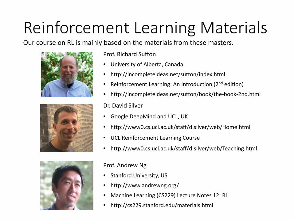
Reinforcement Learning MaterialsProf. Richard Sutton• University of Alberta, Canada• http://incompleteideas.net/sutton/index.html• Reinforcement Learning: An Introduction (2nd edition)• http://incompleteideas.net/sutton/book/the-book-2nd.html

Dr. David Silver• Google DeepMind and UCL, UK

• http://www0.cs.ucl.ac.uk/staff/d.silver/web/Home.html

• UCL Reinforcement Learning Course

• http://www0.cs.ucl.ac.uk/staff/d.silver/web/Teaching.html

Our course on RL is mainly based on the materials from these masters.

Prof. Andrew Ng• Stanford University, US• http://www.andrewng.org/• Machine Learning (CS229) Lecture Notes 12: RL• http://cs229.stanford.edu/materials.html

Last Lecture• Model-based dynamic programming

• Value iteration V (s) = R(s) + maxa2A

°Xs02S

Psa(s0)V (s0)V (s) = R(s) + max

a2A°

Xs02S

Psa(s0)V (s0)

¼(s) = arg maxa2A

Xs02S

Psa(s0)V (s0)¼(s) = arg max

a2A

Xs02S

Psa(s0)V (s0)• Policy iteration

• Model-free reinforcement learning• On-policy MC V (st) Ã V (st) + ®(Gt ¡ V (st))V (st) Ã V (st) + ®(Gt ¡ V (st))

• On-policy TD V (st) Ã V (st) + ®(rt+1 + °V (st+1)¡ V (st))V (st) Ã V (st) + ®(rt+1 + °V (st+1)¡ V (st))

• On-policy TD SARSAQ(st; at) Ã Q(st; at) + ®(rt+1 + °Q(st+1; at+1)¡Q(st; at))Q(st; at) Ã Q(st; at) + ®(rt+1 + °Q(st+1; at+1)¡Q(st; at))

• Off-policy TD Q-learningQ(st; at) Ã Q(st; at) + ®(rt+1 + ° max

a0 Q(st+1; at+1)¡Q(st; at))Q(st; at) Ã Q(st; at) + ®(rt+1 + ° maxa0 Q(st+1; at+1)¡Q(st; at))

Key Problem to Solve in This Lecture

• In all previous models, we have created a lookup table to maintain a variable V(s) for each state or Q(s,a) for each state-action

• What if we have a large MDP, i.e. • the state or state-action space is too large • or the state or action space is continuousto maintain V(s) for each state or Q(s,a) for each state-action? • For example

• Game of Go (10170 states)• Helicopter, autonomous car (continuous state space)

Content• Solutions for large MDPs

• Discretize or bucketize states/actions• Build parametric value function approximation

• Policy gradient

• Deep reinforcement learning and multi-agent RL

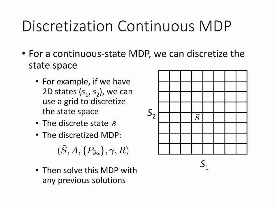
Discretization Continuous MDP• For a continuous-state MDP, we can discretize the

state space• For example, if we have

2D states (s1, s2), we can use a grid to discretize the state space

• The discrete state• The discretized MDP:

S1

S2¹s¹s

¹s¹s

( ¹S; A; fP¹sag; °; R)( ¹S; A; fP¹sag; °; R)

• Then solve this MDP with any previous solutions

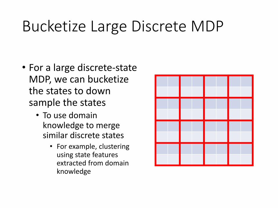
Bucketize Large Discrete MDP

• For a large discrete-state MDP, we can bucketize the states to down sample the states• To use domain

knowledge to merge similar discrete states• For example, clustering

using state features extracted from domain knowledge

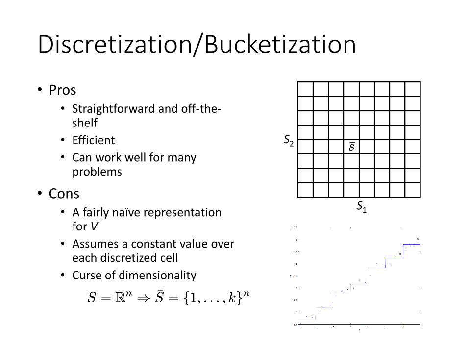
Discretization/Bucketization• Pros

• Straightforward and off-the-shelf

• Efficient• Can work well for many

problems

• Cons• A fairly naïve representation

for V• Assumes a constant value over

each discretized cell• Curse of dimensionality

S1

S2 ¹s¹s

S = Rn ) ¹S = f1; : : : ; kgnS = Rn ) ¹S = f1; : : : ; kgn

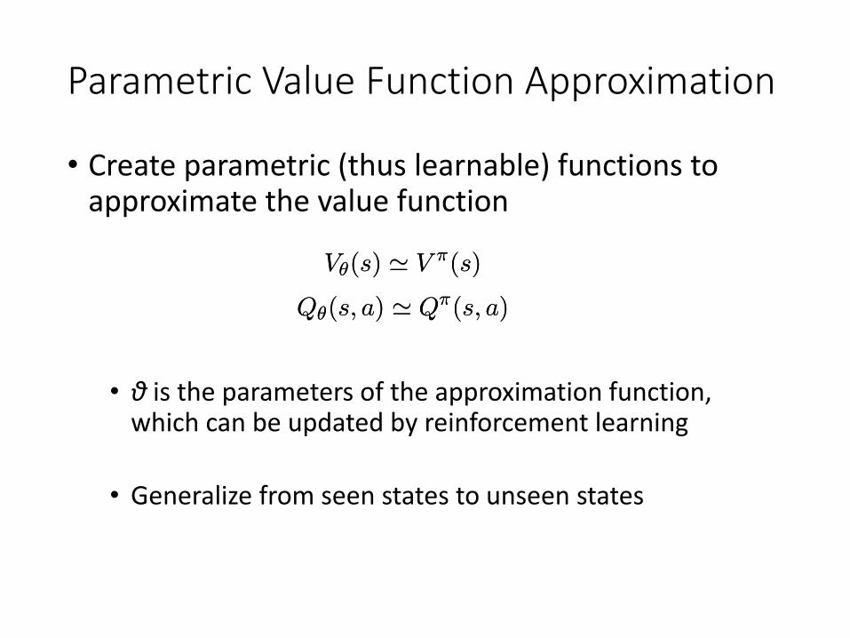
Parametric Value Function Approximation

• Create parametric (thus learnable) functions to approximate the value function

Vμ(s) ' V ¼(s)Vμ(s) ' V ¼(s)

Qμ(s; a) ' Q¼(s; a)Qμ(s; a) ' Q¼(s; a)

• θ is the parameters of the approximation function, which can be updated by reinforcement learning

• Generalize from seen states to unseen states

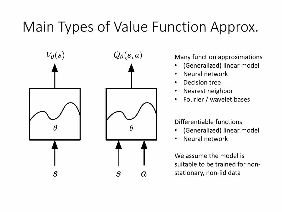
Main Types of Value Function Approx.

Vμ(s)Vμ(s) Qμ(s; a)Qμ(s; a)

ss ss aa

μμ μμ

Many function approximations• (Generalized) linear model• Neural network• Decision tree• Nearest neighbor• Fourier / wavelet bases

Differentiable functions• (Generalized) linear model• Neural network

We assume the model is suitable to be trained for non-stationary, non-iid data

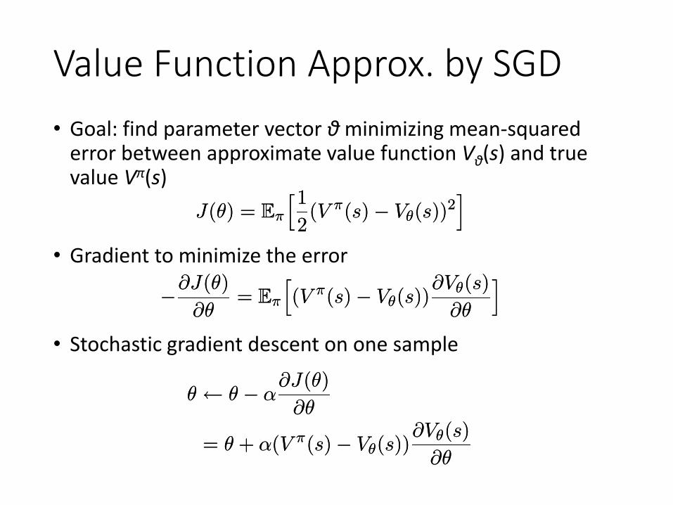
Value Function Approx. by SGD• Goal: find parameter vector θ minimizing mean-squared

error between approximate value function Vθ(s) and true value Vπ(s)

J(μ) = E¼

h1

2(V ¼(s)¡ Vμ(s))

2i

J(μ) = E¼

h1

2(V ¼(s)¡ Vμ(s))

2i

• Gradient to minimize the error

¡@J(μ)

@μ= E¼

h(V ¼(s)¡ Vμ(s))

@Vμ(s)

@μ

i¡@J(μ)

@μ= E¼

h(V ¼(s)¡ Vμ(s))

@Vμ(s)

@μ

i• Stochastic gradient descent on one sample

μ Ã μ ¡ ®@J(μ)

@μ

= μ + ®(V ¼(s)¡ Vμ(s))@Vμ(s)

@μ

μ Ã μ ¡ ®@J(μ)

@μ

= μ + ®(V ¼(s)¡ Vμ(s))@Vμ(s)

@μ

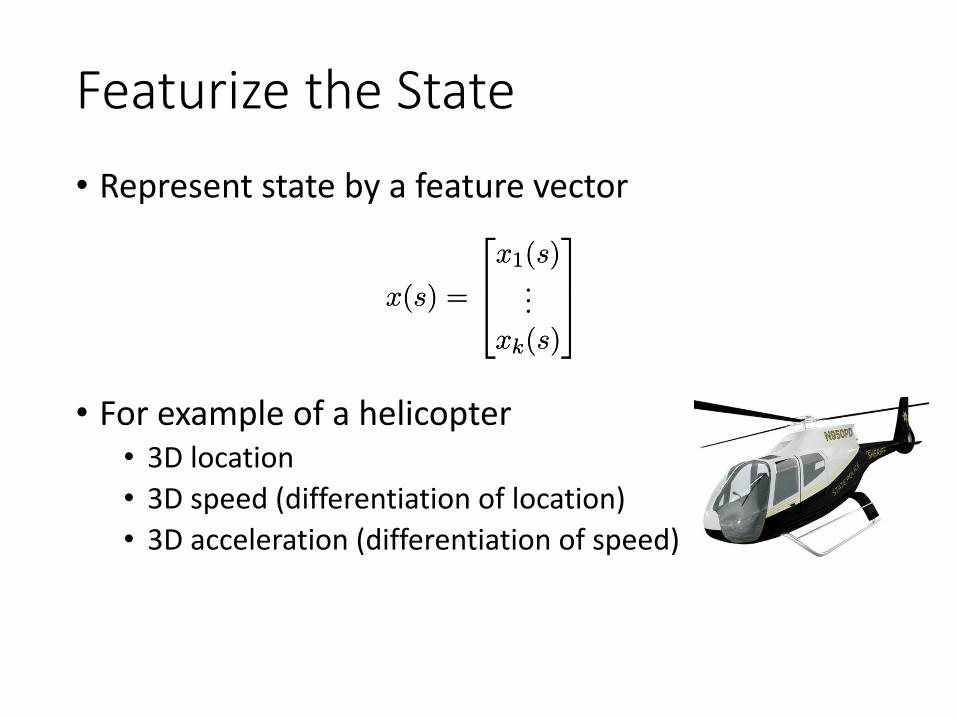
Featurize the State• Represent state by a feature vector

x(s) =

264x1(s)...

xk(s)

375x(s) =

264x1(s)...

xk(s)

375• For example of a helicopter

• 3D location• 3D speed (differentiation of location)• 3D acceleration (differentiation of speed)

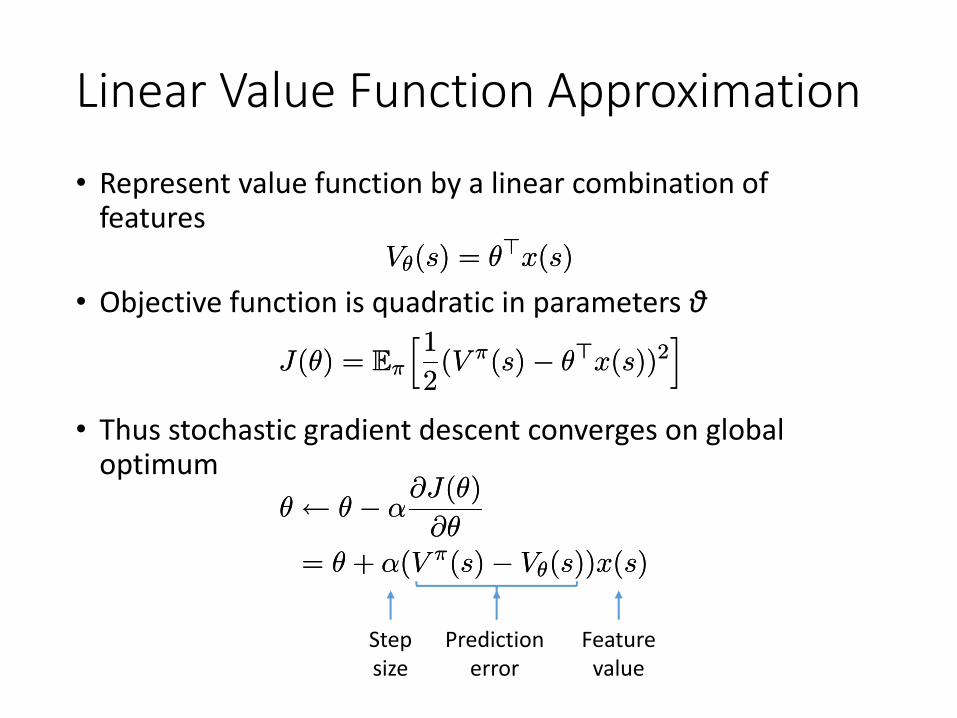
Linear Value Function Approximation

• Represent value function by a linear combination of features

Vμ(s) = μ>x(s)Vμ(s) = μ>x(s)

• Objective function is quadratic in parameters θ

J(μ) = E¼

h1

2(V ¼(s)¡ μ>x(s))2

iJ(μ) = E¼

h1

2(V ¼(s)¡ μ>x(s))2

i• Thus stochastic gradient descent converges on global

optimumμ Ã μ ¡ ®

@J(μ)

@μ= μ + ®(V ¼(s)¡ Vμ(s))x(s)

μ Ã μ ¡ ®@J(μ)

@μ= μ + ®(V ¼(s)¡ Vμ(s))x(s)

Stepsize

Predictionerror

Featurevalue

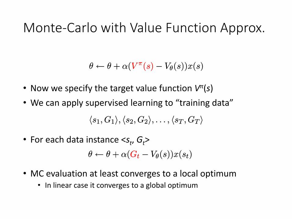
Monte-Carlo with Value Function Approx.

• Now we specify the target value function Vπ(s)• We can apply supervised learning to “training data”

μ Ã μ + ®(V ¼(s)¡ Vμ(s))x(s)μ Ã μ + ®(V ¼(s)¡ Vμ(s))x(s)

hs1; G1i; hs2; G2i; : : : ; hsT ; GT ihs1; G1i; hs2; G2i; : : : ; hsT ; GT i

μ Ã μ + ®(Gt ¡ Vμ(s))x(st)μ Ã μ + ®(Gt ¡ Vμ(s))x(st)

• For each data instance <st, Gt>

• MC evaluation at least converges to a local optimum• In linear case it converges to a global optimum

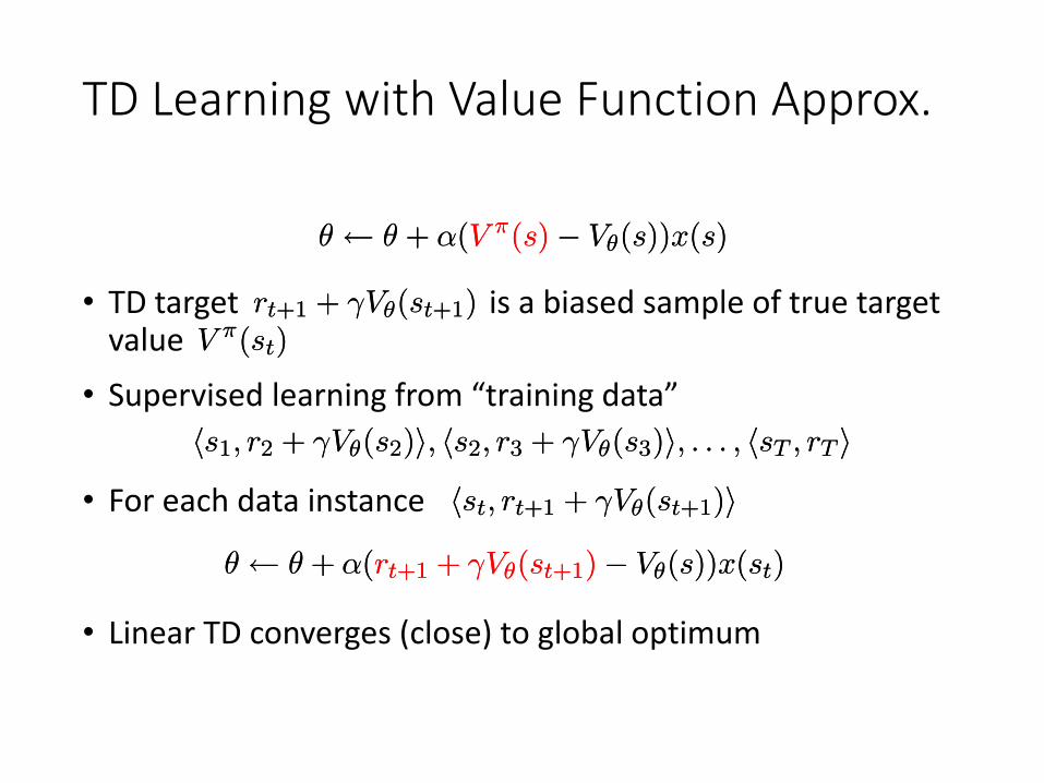
TD Learning with Value Function Approx.

• TD target is a biased sample of true target value

μ Ã μ + ®(V ¼(s)¡ Vμ(s))x(s)μ Ã μ + ®(V ¼(s)¡ Vμ(s))x(s)

rt+1 + °Vμ(st+1)rt+1 + °Vμ(st+1)V ¼(st)V ¼(st)

• Supervised learning from “training data”hs1; r2 + °Vμ(s2)i; hs2; r3 + °Vμ(s3)i; : : : ; hsT ; rT ihs1; r2 + °Vμ(s2)i; hs2; r3 + °Vμ(s3)i; : : : ; hsT ; rT i

• For each data instance hst; rt+1 + °Vμ(st+1)ihst; rt+1 + °Vμ(st+1)iμÃ μ + ®(rt+1 + °Vμ(st+1)¡ Vμ(s))x(st)μÃ μ + ®(rt+1 + °Vμ(st+1)¡ Vμ(s))x(st)

• Linear TD converges (close) to global optimum

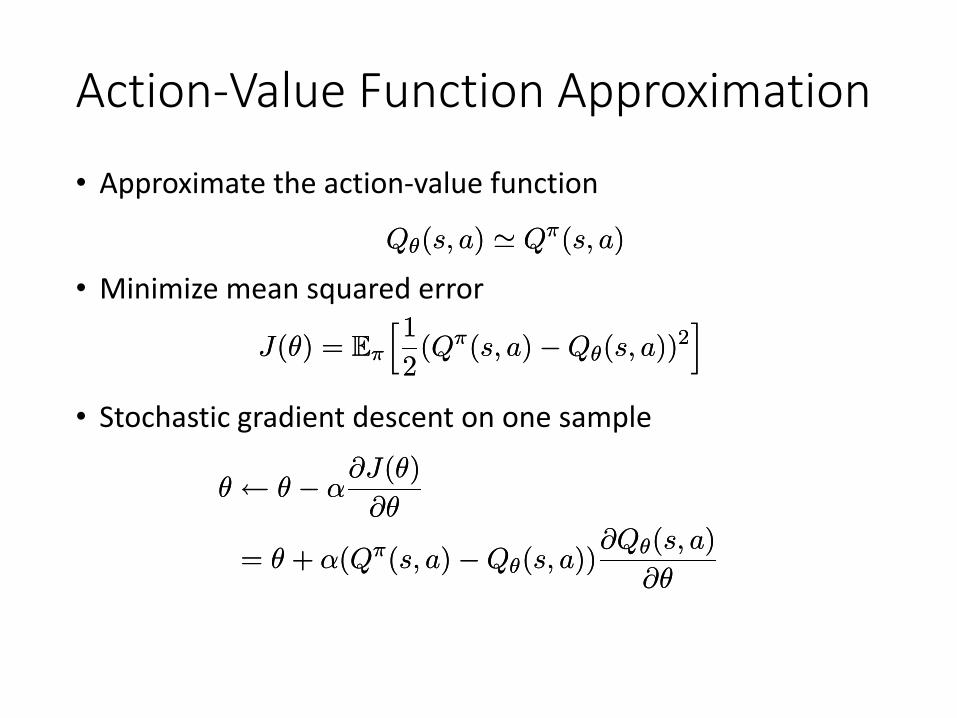
Action-Value Function Approximation

• Approximate the action-value function

Qμ(s; a) ' Q¼(s; a)Qμ(s; a) ' Q¼(s; a)

• Minimize mean squared error

J(μ) = E¼

h1

2(Q¼(s; a)¡Qμ(s; a))2

iJ(μ) = E¼

h1

2(Q¼(s; a)¡Qμ(s; a))2

i• Stochastic gradient descent on one sample

μ Ã μ ¡ ®@J(μ)

@μ

= μ + ®(Q¼(s; a)¡Qμ(s; a))@Qμ(s; a)

@μ

μ Ã μ ¡ ®@J(μ)

@μ

= μ + ®(Q¼(s; a)¡Qμ(s; a))@Qμ(s; a)

@μ

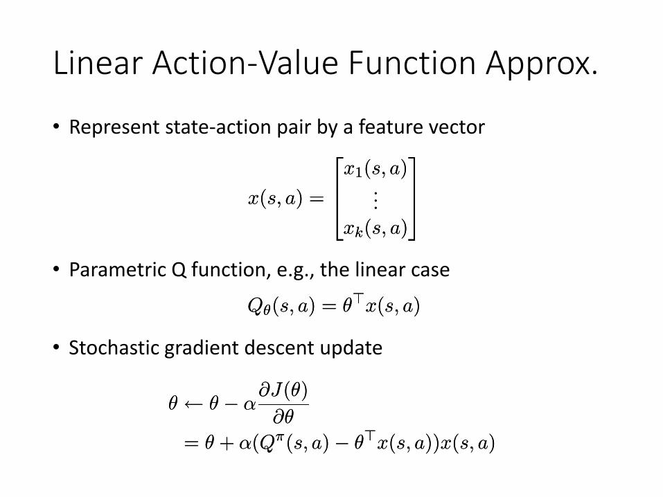
Linear Action-Value Function Approx.

• Represent state-action pair by a feature vector

x(s; a) =

264x1(s; a)...

xk(s; a)

375x(s; a) =

264x1(s; a)...

xk(s; a)

375• Parametric Q function, e.g., the linear case

Qμ(s; a) = μ>x(s; a)Qμ(s; a) = μ>x(s; a)

• Stochastic gradient descent update

μ Ã μ ¡ ®@J(μ)

@μ

= μ + ®(Q¼(s; a)¡ μ>x(s; a))x(s; a)

μ Ã μ ¡ ®@J(μ)

@μ

= μ + ®(Q¼(s; a)¡ μ>x(s; a))x(s; a)

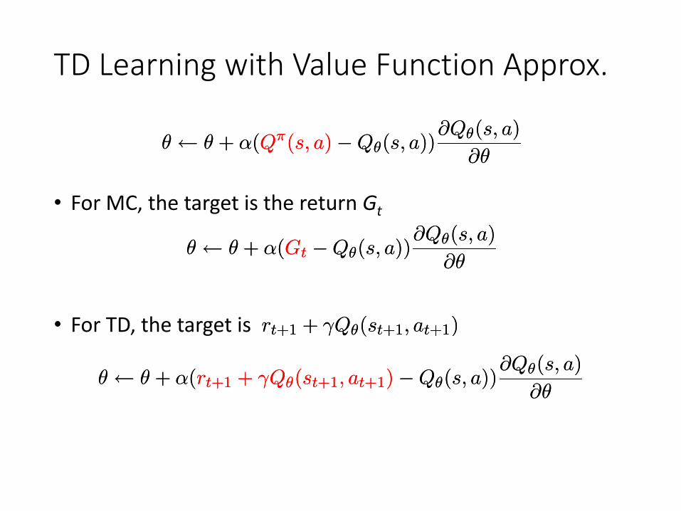
TD Learning with Value Function Approx.

• For MC, the target is the return Gt

rt+1 + °Qμ(st+1; at+1)rt+1 + °Qμ(st+1; at+1)• For TD, the target is

μ Ã μ + ®(Q¼(s; a)¡Qμ(s; a))@Qμ(s; a)

@μμ Ã μ + ®(Q¼(s; a)¡Qμ(s; a))

@Qμ(s; a)

@μ

μ Ã μ + ®(Gt ¡Qμ(s; a))@Qμ(s; a)

@μμ Ã μ + ®(Gt ¡Qμ(s; a))

@Qμ(s; a)

@μ

μ Ã μ + ®(rt+1 + °Qμ(st+1; at+1)¡Qμ(s; a))@Qμ(s; a)

@μμ Ã μ + ®(rt+1 + °Qμ(st+1; at+1)¡Qμ(s; a))

@Qμ(s; a)

@μ

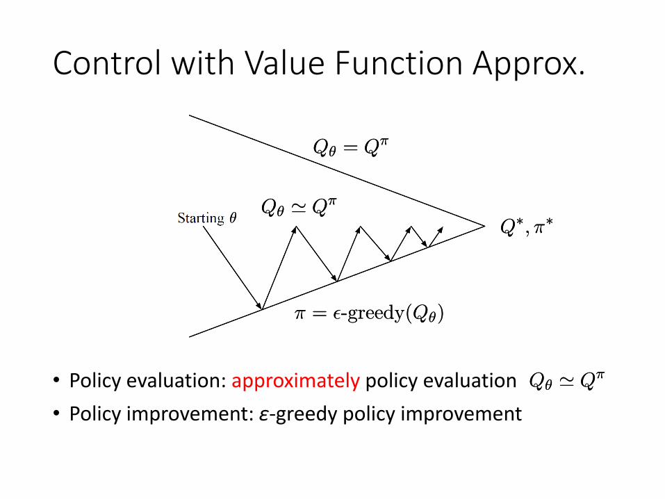
Control with Value Function Approx.

Qμ = Q¼Qμ = Q¼

¼ = ²-greedy(Qμ)¼ = ²-greedy(Qμ)

μμQ¤; ¼¤Q¤; ¼¤

• Policy evaluation: approximately policy evaluation• Policy improvement: ɛ-greedy policy improvement

Qμ ' Q¼Qμ ' Q¼

Qμ ' Q¼Qμ ' Q¼

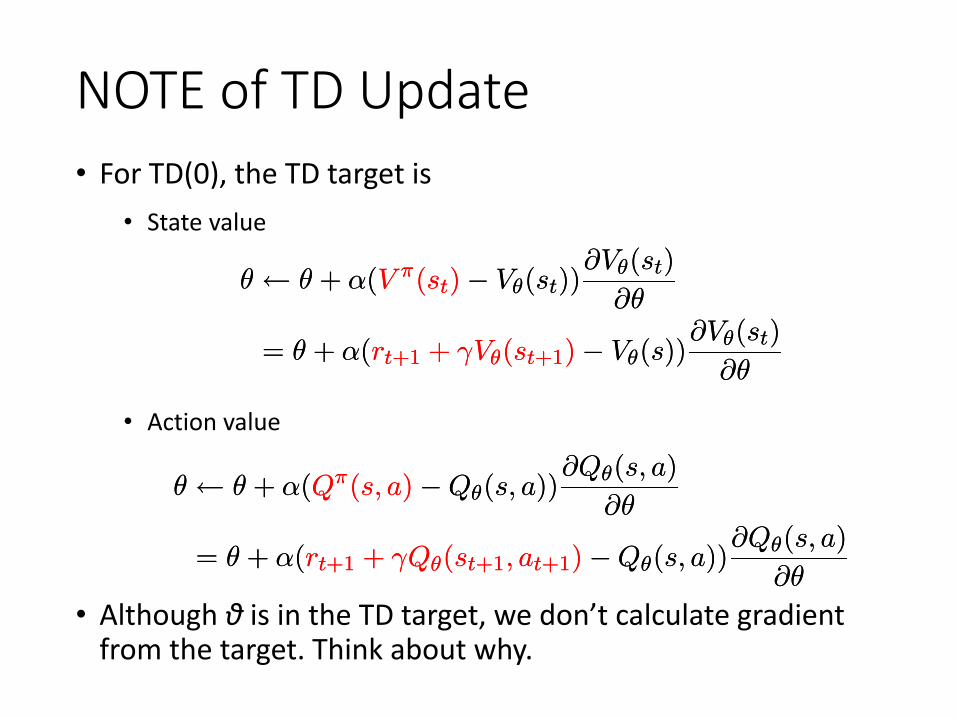
NOTE of TD Update• For TD(0), the TD target is

μ Ã μ + ®(V ¼(st)¡ Vμ(st))@Vμ(st)

@μ

= μ + ®(rt+1 + °Vμ(st+1)¡ Vμ(s))@Vμ(st)

@μ

μ Ã μ + ®(V ¼(st)¡ Vμ(st))@Vμ(st)

@μ

= μ + ®(rt+1 + °Vμ(st+1)¡ Vμ(s))@Vμ(st)

@μ

• State value

• Action value

μ Ã μ + ®(Q¼(s; a)¡Qμ(s; a))@Qμ(s; a)

@μ

= μ + ®(rt+1 + °Qμ(st+1; at+1)¡Qμ(s; a))@Qμ(s; a)

@μ

μ Ã μ + ®(Q¼(s; a)¡Qμ(s; a))@Qμ(s; a)

@μ

= μ + ®(rt+1 + °Qμ(st+1; at+1)¡Qμ(s; a))@Qμ(s; a)

@μ

• Although θ is in the TD target, we don’t calculate gradient from the target. Think about why.

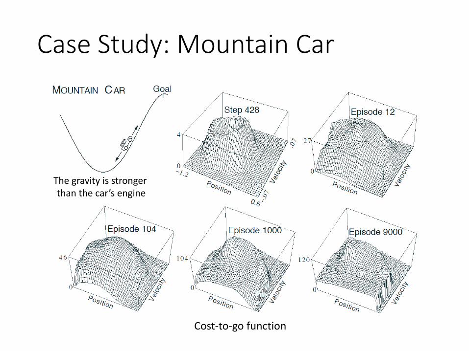
Case Study: Mountain Car

The gravity is stronger than the car’s engine

Cost-to-go function

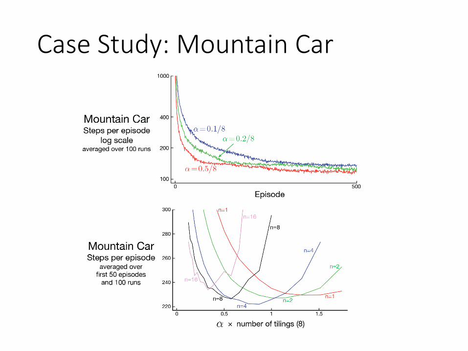
Case Study: Mountain Car

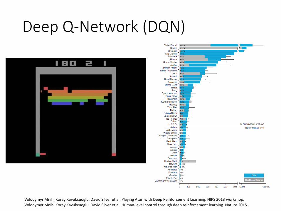
Deep Q-Network (DQN)

Volodymyr Mnih, Koray Kavukcuoglu, David Silver et al. Human-level control through deep reinforcement learning. Nature 2015.Volodymyr Mnih, Koray Kavukcuoglu, David Silver et al. Playing Atari with Deep Reinforcement Learning. NIPS 2013 workshop.

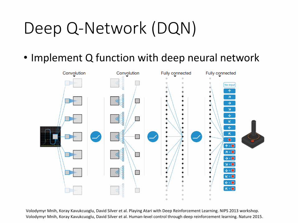
Deep Q-Network (DQN)• Implement Q function with deep neural network

Volodymyr Mnih, Koray Kavukcuoglu, David Silver et al. Human-level control through deep reinforcement learning. Nature 2015.Volodymyr Mnih, Koray Kavukcuoglu, David Silver et al. Playing Atari with Deep Reinforcement Learning. NIPS 2013 workshop.

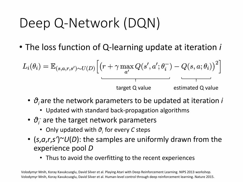
Deep Q-Network (DQN)• The loss function of Q-learning update at iteration i

Volodymyr Mnih, Koray Kavukcuoglu, David Silver et al. Human-level control through deep reinforcement learning. Nature 2015.

Li(μi) = E(s;a;r;s0)»U(D)

h¡r + ° max

a0 Q(s0; a0; μ¡i )¡Q(s; a; μi)¢2

iLi(μi) = E(s;a;r;s0)»U(D)

h¡r + ° max

a0 Q(s0; a0; μ¡i )¡Q(s; a; μi)¢2

i

• θi are the network parameters to be updated at iteration i• Updated with standard back-propagation algorithms

• θi- are the target network parameters• Only updated with θi for every C steps

• (s,a,r,s’)~U(D): the samples are uniformly drawn from the experience pool D• Thus to avoid the overfitting to the recent experiences

target Q value estimated Q value

Volodymyr Mnih, Koray Kavukcuoglu, David Silver et al. Playing Atari with Deep Reinforcement Learning. NIPS 2013 workshop.



• Policy gradient

• Deep reinforcement learning and multi-agent RL

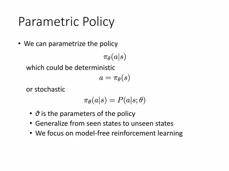
Parametric Policy• We can parametrize the policy

• θ is the parameters of the policy• Generalize from seen states to unseen states• We focus on model-free reinforcement learning

¼μ(ajs)¼μ(ajs)which could be deterministic

a = ¼μ(s)a = ¼μ(s)

or stochastic¼μ(ajs) = P (ajs; μ)¼μ(ajs) = P (ajs; μ)

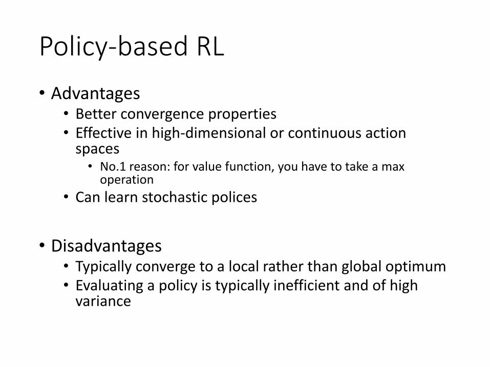
Policy-based RL• Advantages

• Better convergence properties• Effective in high-dimensional or continuous action

spaces• No.1 reason: for value function, you have to take a max

operation• Can learn stochastic polices

• Disadvantages• Typically converge to a local rather than global optimum• Evaluating a policy is typically inefficient and of high

variance

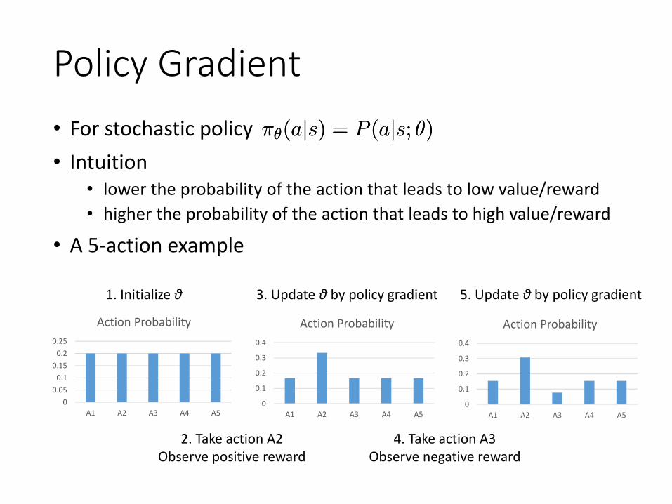
Policy Gradient• For stochastic policy• Intuition

• lower the probability of the action that leads to low value/reward• higher the probability of the action that leads to high value/reward

• A 5-action example

¼μ(ajs) = P (ajs; μ)¼μ(ajs) = P (ajs; μ)

00.05

0.10.15

0.20.25

A1 A2 A3 A4 A5

Action Probability

0

0.1

0.2

0.3

0.4

A1 A2 A3 A4 A5

Action Probability

0

0.1

0.2

0.3

0.4

A1 A2 A3 A4 A5

Action Probability

2. Take action A2Observe positive reward

4. Take action A3Observe negative reward

1. Initialize θ 3. Update θ by policy gradient 5. Update θ by policy gradient

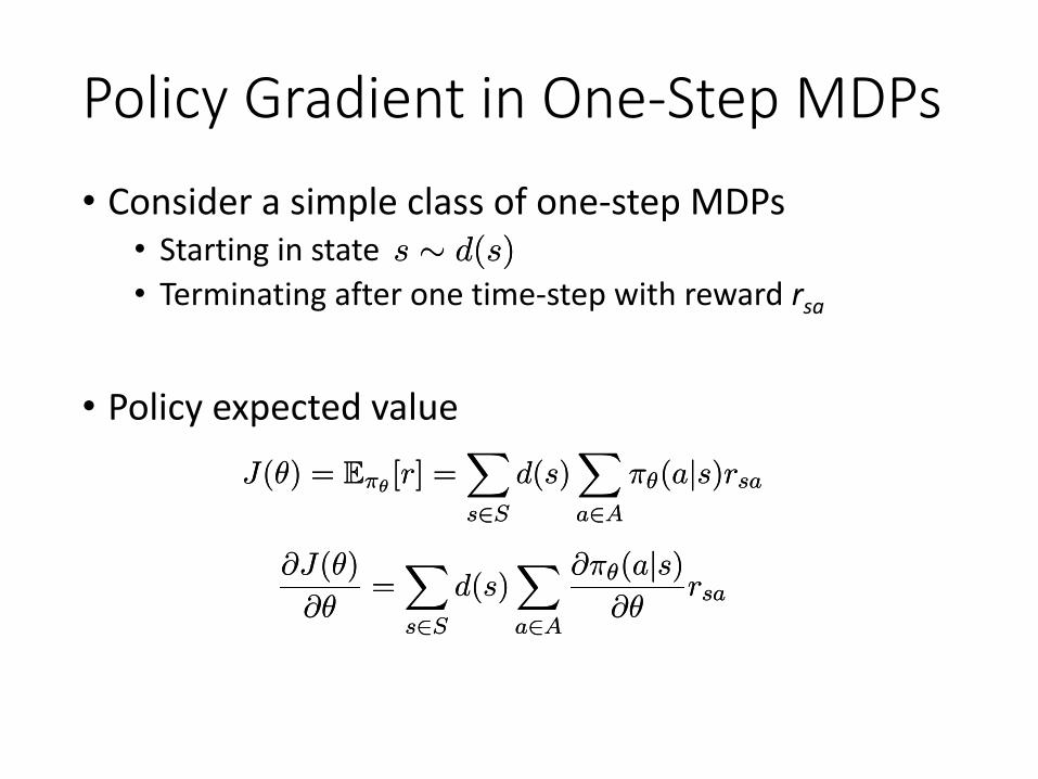
Policy Gradient in One-Step MDPs• Consider a simple class of one-step MDPs

• Starting in state• Terminating after one time-step with reward rsa

• Policy expected value

s » d(s)s » d(s)

J(μ) = E¼μ [r] =Xs2S

d(s)Xa2A

¼μ(ajs)rsaJ(μ) = E¼μ [r] =Xs2S

d(s)Xa2A

¼μ(ajs)rsa

@J(μ)

@μ=

Xs2S

d(s)Xa2A

@¼μ(ajs)@μ

rsa@J(μ)

@μ=

Xs2S

d(s)Xa2A

@¼μ(ajs)@μ

rsa

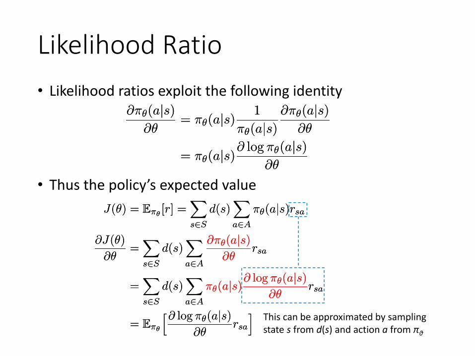
Likelihood Ratio• Likelihood ratios exploit the following identity

@¼μ(ajs)@μ

= ¼μ(ajs) 1

¼μ(ajs)@¼μ(ajs)

@μ

= ¼μ(ajs)@ log ¼μ(ajs)@μ

@¼μ(ajs)@μ

= ¼μ(ajs) 1

¼μ(ajs)@¼μ(ajs)

@μ

= ¼μ(ajs)@ log ¼μ(ajs)@μ

• Thus the policy’s expected valueJ(μ) = E¼μ [r] =

Xs2S

d(s)Xa2A

¼μ(ajs)rsaJ(μ) = E¼μ [r] =Xs2S

d(s)Xa2A

¼μ(ajs)rsa

@J(μ)

@μ=

Xs2S

d(s)Xa2A

@¼μ(ajs)@μ

rsa

=Xs2S

d(s)Xa2A

¼μ(ajs)@ log ¼μ(ajs)@μ

rsa

= E¼μ

h@ log ¼μ(ajs)@μ

rsa

i

@J(μ)

@μ=

Xs2S

d(s)Xa2A

@¼μ(ajs)@μ

rsa

=Xs2S

d(s)Xa2A

¼μ(ajs)@ log ¼μ(ajs)@μ

rsa

= E¼μ

h@ log ¼μ(ajs)@μ

rsa

i This can be approximated by sampling state s from d(s) and action a from πθ

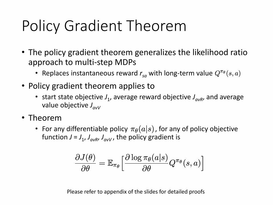
Policy Gradient Theorem• The policy gradient theorem generalizes the likelihood ratio

approach to multi-step MDPs• Replaces instantaneous reward rsa with long-term value

• Policy gradient theorem applies to • start state objective J1, average reward objective JavR, and average

value objective JavV• Theorem

• For any differentiable policy , for any of policy objective function J = J1, JavR, JavV , the policy gradient is

Q¼μ(s; a)Q¼μ(s; a)

¼μ(ajs)¼μ(ajs)

@J(μ)

@μ= E¼μ

h@ log ¼μ(ajs)@μ

Q¼μ(s; a)i@J(μ)

@μ= E¼μ

h@ log ¼μ(ajs)@μ

Q¼μ(s; a)i

Please refer to appendix of the slides for detailed proofs

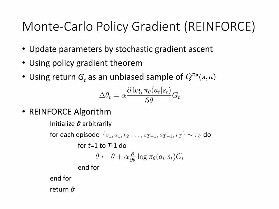
Monte-Carlo Policy Gradient (REINFORCE)• Update parameters by stochastic gradient ascent• Using policy gradient theorem• Using return Gt as an unbiased sample of Q¼μ(s; a)Q¼μ(s; a)

¢μt = ®@ log ¼μ(atjst)

@μGt

• REINFORCE AlgorithmInitialize θ arbitrarilyfor each episode do

for t=1 to T-1 do

end forend forreturn θ

fs1; a1; r2; : : : ; sT¡1; aT¡1; rTg » ¼μ

μ Ã μ + ® @@μ

log ¼μ(atjst)Gt

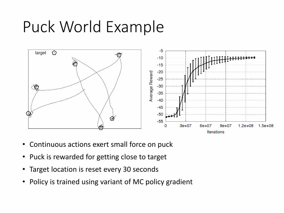
Puck World Example

• Continuous actions exert small force on puck• Puck is rewarded for getting close to target• Target location is reset every 30 seconds• Policy is trained using variant of MC policy gradient

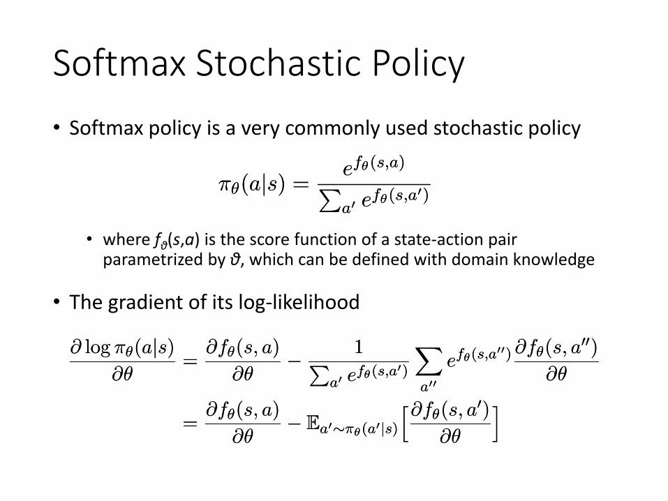
Softmax Stochastic Policy• Softmax policy is a very commonly used stochastic policy

¼μ(ajs) =efμ(s;a)Pa0 efμ(s;a0)¼μ(ajs) =efμ(s;a)Pa0 efμ(s;a0)

• where fθ(s,a) is the score function of a state-action pair parametrized by θ, which can be defined with domain knowledge

@ log ¼μ(ajs)@μ

=@fμ(s; a)

@μ¡ 1P

a0 efμ(s;a0)

Xa00

efμ(s;a00) @fμ(s; a

00)@μ

=@fμ(s; a)

@μ¡ Ea0»¼μ(a0js)

h@fμ(s; a0)

@μ

i@ log ¼μ(ajs)

@μ=

@fμ(s; a)

@μ¡ 1P

a0 efμ(s;a0)

Xa00

efμ(s;a00) @fμ(s; a

00)@μ

=@fμ(s; a)


h@fμ(s; a0)

@μ

i

• The gradient of its log-likelihood

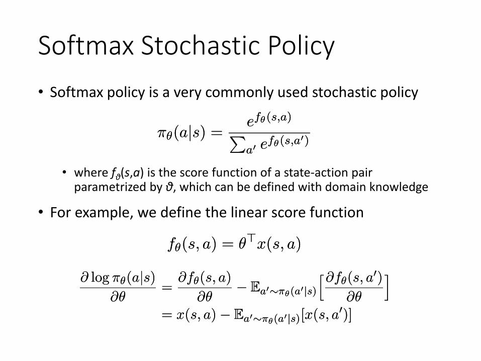
Softmax Stochastic Policy• Softmax policy is a very commonly used stochastic policy

¼μ(ajs) =efμ(s;a)Pa0 efμ(s;a0)¼μ(ajs) =efμ(s;a)Pa0 efμ(s;a0)

• where fθ(s,a) is the score function of a state-action pair parametrized by θ, which can be defined with domain knowledge

• For example, we define the linear score function

fμ(s; a) = μ>x(s; a)fμ(s; a) = μ>x(s; a)

@ log ¼μ(ajs)@μ

=@fμ(s; a)


h@fμ(s; a0)

@μ

i= x(s; a)¡ Ea0»¼μ(a0js)[x(s; a0)]

@ log ¼μ(ajs)@μ

=@fμ(s; a)


h@fμ(s; a0)

@μ

i= x(s; a)¡ Ea0»¼μ(a0js)[x(s; a0)]

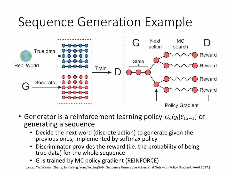
Sequence Generation Example

• Generator is a reinforcement learning policy of generating a sequence• Decide the next word (discrete action) to generate given the

previous ones, implemented by softmax policy• Discriminator provides the reward (i.e. the probability of being

true data) for the whole sequence• G is trained by MC policy gradient (REINFORCE)

Gμ(ytjY1:t¡1)Gμ(ytjY1:t¡1)

[Lantao Yu, Weinan Zhang, Jun Wang, Yong Yu. SeqGAN: Sequence Generative Adversarial Nets with Policy Gradient. AAAI 2017.]

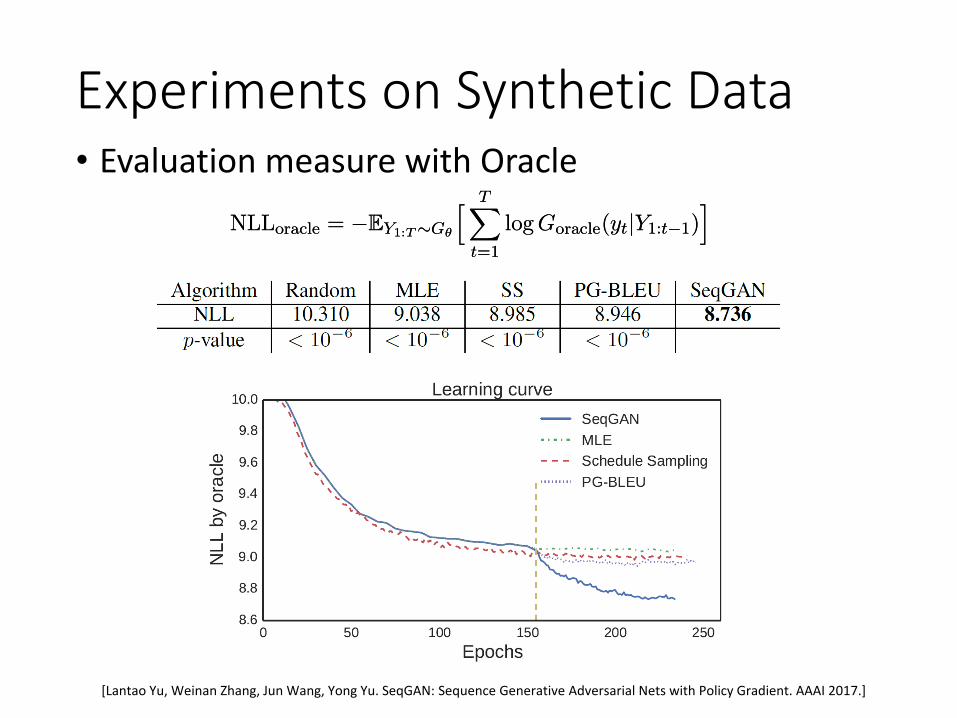
Experiments on Synthetic Data• Evaluation measure with Oracle

NLLoracle = ¡EY1:T»Gμ

h TXt=1

log Goracle(ytjY1:t¡1)i

NLLoracle = ¡EY1:T»Gμ

h TXt=1

log Goracle(ytjY1:t¡1)i

[Lantao Yu, Weinan Zhang, Jun Wang, Yong Yu. SeqGAN: Sequence Generative Adversarial Nets with Policy Gradient. AAAI 2017.]



• Policy gradient

• Deep reinforcement learning and multi-agent RL• By our invited speakers Yuhuai Wu, Shixiang Gu and Ying

Wen

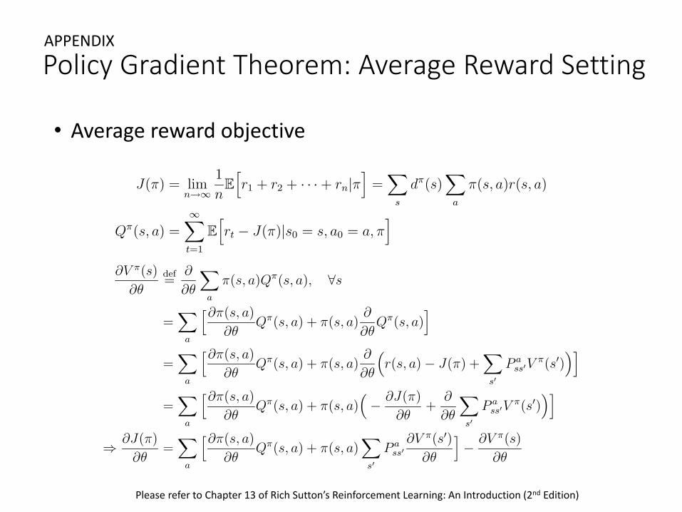
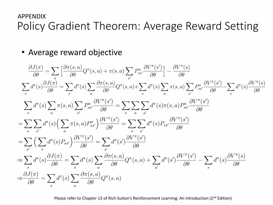
Policy Gradient Theorem: Average Reward Setting

J(¼) = limn!1

1

nE

hr1 + r2 + ¢ ¢ ¢+ rnj¼

i=

Xs

d¼(s)X

a

¼(s; a)r(s; a)

Q¼(s; a) =

1Xt=1

Ehrt ¡ J(¼)js0 = s; a0 = a; ¼

i@V ¼(s)

@μ

def=

@

@μ

Xa

¼(s; a)Q¼(s; a); 8s

=X

a

h@¼(s; a)

@μQ¼(s; a) + ¼(s; a)

@

@μQ¼(s; a)

i=

Xa

h@¼(s; a)

@μQ¼(s; a) + ¼(s; a)

@

@μ

³r(s; a)¡ J(¼) +

Xs0

P ass0V ¼(s0)

´i=

Xa

h@¼(s; a)

@μQ¼(s; a) + ¼(s; a)

³¡ @J(¼)

@μ+

@

@μ

Xs0

P ass0V ¼(s0)

´i) @J(¼)

@μ=

Xa

h@¼(s; a)

@μQ¼(s; a) + ¼(s; a)

Xs0

P ass0

@V ¼(s0)@μ

i¡ @V ¼(s)

@μ

• Average reward objective

APPENDIX

Please refer to Chapter 13 of Rich Sutton’s Reinforcement Learning: An Introduction (2nd Edition)

@J(¼)

@μ=

Xa

h@¼(s; a)

@μQ¼(s; a) + ¼(s; a)

Xs0

P ass0

@V ¼(s0)@μ

i¡ @V ¼(s)

@μXs

d¼(s)@J(¼)

@μ=

Xs

d¼(s)X

a

@¼(s; a)

@μQ¼(s; a)+

Xs

d¼(s)X

a

¼(s; a)X

s0P a

ss0@V ¼(s0)

@μ¡

Xs

d¼(s)@V ¼(s)

@μXs

d¼(s)X

a

¼(s; a)Xs0

P ass0

@V ¼(s0)@μ

=X

s

Xa

Xs0

d¼(s)¼(s; a)P ass0

@V ¼(s0)@μ

=X

s

Xs0

d¼(s)³ X

a

¼(s; a)P ass0

´@V ¼(s0)@μ

=X

s

Xs0

d¼(s)Pss0@V ¼(s0)

@μ

=Xs0

³Xs

d¼(s)Pss0´@V ¼(s0)

@μ=

Xs0

d¼(s0)@V ¼(s0)

@μ

)X

s

d¼(s)@J(¼)

@μ=

Xs

d¼(s)X

a

@¼(s; a)

@μQ¼(s; a) +

Xs0

d¼(s0)@V ¼(s0)

@μ¡

Xs

d¼(s)@V ¼(s)

@μ

)@J(¼)

@μ=

Xs

d¼(s)X

a

@¼(s; a)

@μQ¼(s; a)

Policy Gradient Theorem: Average Reward Setting

• Average reward objective

APPENDIX


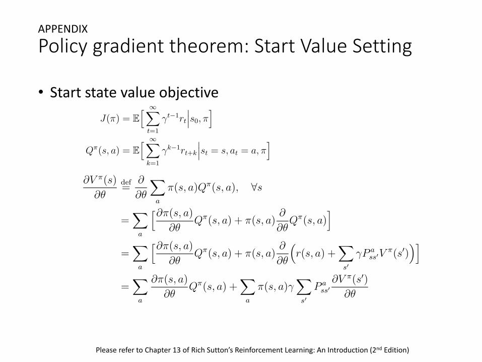
Policy gradient theorem: Start Value Setting

J(¼) = Eh 1X

t=1

°t¡1rt

¯̄̄s0; ¼

iQ¼(s; a) = E

h 1Xk=1

°k¡1rt+k

¯̄̄st = s; at = a; ¼

i@V ¼(s)

@μdef=

@

@μ

Xa

¼(s; a)Q¼(s; a); 8s

=X

a

h@¼(s; a)

@μQ¼(s; a) + ¼(s; a)

@

@μQ¼(s; a)

i=

Xa

h@¼(s; a)

@μQ¼(s; a) + ¼(s; a)

@

@μ

³r(s; a) +

Xs0

°P ass0V ¼(s0)

´i=

Xa

@¼(s; a)

@μQ¼(s; a) +

Xa

¼(s; a)°Xs0

P ass0

@V ¼(s0)@μ

APPENDIX

• Start state value objective


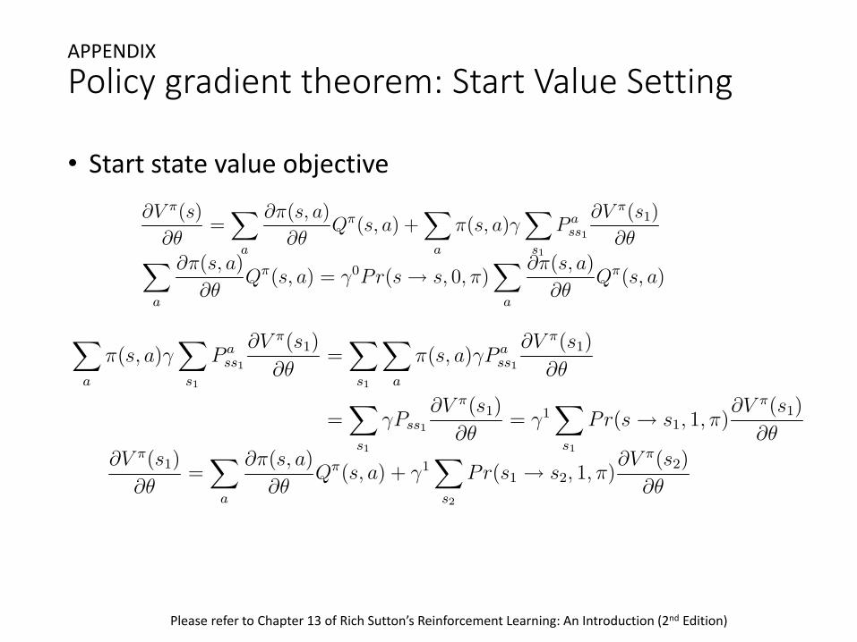
Policy gradient theorem: Start Value SettingAPPENDIX

• Start state value objective@V ¼(s)

@μ=

Xa

@¼(s; a)

@μQ¼(s; a) +

Xa

¼(s; a)°Xs1

P ass1

@V ¼(s1)

@μXa

@¼(s; a)

@μQ¼(s; a) = °0Pr(s ! s; 0; ¼)

Xa

@¼(s; a)

@μQ¼(s; a)

Xa

¼(s; a)°Xs1

P ass1

@V ¼(s1)

@μ=

Xs1

Xa

¼(s; a)°P ass1

@V ¼(s1)

@μ

=Xs1

°Pss1

@V ¼(s1)

@μ= °1

Xs1

Pr(s ! s1; 1; ¼)@V ¼(s1)

@μ@V ¼(s1)

@μ=

Xa

@¼(s; a)

@μQ¼(s; a) + °1

Xs2

Pr(s1 ! s2; 1; ¼)@V ¼(s2)

@μ


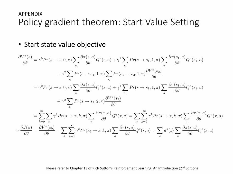
Policy gradient theorem: Start Value SettingAPPENDIX

• Start state value objective@V ¼(s)

@μ= °0Pr(s ! s; 0; ¼)

Xa

@¼(s; a)

@μQ¼(s; a) + °1

Xs1

Pr(s ! s1; 1; ¼)X

a

@¼(s1; a)

@μQ¼(s1; a)

+ °2Xs1

Pr(s ! s1; 1; ¼)Xs2

Pr(s1 ! s2; 1; ¼)@V ¼(s2)

@μ

= °0Pr(s ! s; 0; ¼)X

a

@¼(s; a)

@μQ¼(s; a) + °1

Xs1

Pr(s ! s1; 1; ¼)X

a

@¼(s1; a)

@μQ¼(s1; a)

+ °2Xs2

Pr(s ! s2; 2; ¼)@V ¼(s2)

@μ

=1X

k=0

Xx

°kPr(s ! x; k; ¼)X

a

@¼(x; a)

@μQ¼(x; a) =

Xx

1Xk=0

°kPr(s ! x; k; ¼)X

a

@¼(x; a)

@μQ¼(x; a)

) @J(¼)

@μ=

@V ¼(s0)

@μ=

Xs

1Xk=0

°kPr(s0 ! s; k; ¼)X

a

@¼(s; a)

@μQ¼(s; a) =

Xs

d¼(s)X

a

@¼(s; a)

@μQ¼(s; a)


approximation methods in reinforcement...

Documents