approximation methods for the dynamics in deparametrized lqg
TRANSCRIPT

Mehdi Assanioussi
Faculty of Physics, University of Warsaw
work in collaboration with J. Lewandowski & I. Mäkinen
[arXiv:1702.01688]
Fifth Tux workshop on QG
Tux, Feb 2017
Approximation methods for the
dynamics in Deparametrized LQG

Plan of the talk
I. LQG deparametrized models
II. Physical Hamiltonian operators
III. Approximation methods for the dynamics
i. Expansion: Hamiltonian op. / Evolution op.
ii. Examples
IV. Summary & outlook

LQG deparametrized models

LQG deparametrized models
Motivation
1
• Test-ground for LQG quantization methods
• Insights on the continuum limit of LQG
• Insights on the dynamics of Matter fields in presence of QG

LQG deparametrized models
• Complete quantum gravity models:
* Physical Hilbert space
* Admissible Hamiltonian operator
• Computable dynamics (time evolution)
Motivation
1
• Test-ground for LQG quantization methods
• Insights on the continuum limit of LQG
• Insights on the dynamics of Matter fields in presence of QG
First steps…

LQG deparametrized models
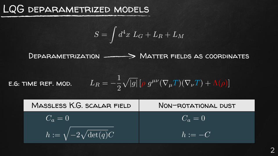
Deparametrization Matter fields as coordinates
2
LQG deparametrized models
Massless K.G. scalar field Non-rotational dust
Deparametrization Matter fields as coordinates
e.g: time ref. mod.
2

Deparametrization
LQG deparametrized models
Time ref. models
Spacetime ref.
models
3

Deparametrization
LQG deparametrized models
Time ref. models
Spacetime ref.
models
Successful
Unsuccessful
3
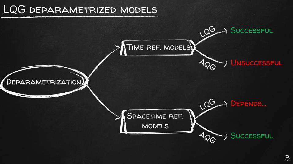
Deparametrization
LQG deparametrized models
Time ref. models
Spacetime ref.
models
Successful
Unsuccessful
Depends…
Successful
3

Deparametrization
LQG deparametrized models
Time ref. models
Spacetime ref.
models
Successful
Unsuccessful
Depends…
Successful
3

LQG deparametrized models
Massless K.G. scalar field Non-rotational dust
e.g: time ref. mod.
4

LQG deparametrized models
Massless K.G. scalar field Non-rotational dust
e.g: time ref. mod.
4
Physical Hilbert space:

LQG deparametrized models
Massless K.G. scalar field Non-rotational dust
e.g: time ref. mod.
4
Proper implementation of the functional C
* Self-adjoint Hamiltonian operator
* Spatial diffeomorphism invariant
* Computable dynamics
Physical Hilbert space:

Physical Hamiltonian operators

Physical Hamiltonian operators
Scalar constraint functional
5
Immirzi-Barbero
parameter

Physical Hamiltonian operators
Scalar constraint functional
Lorentzian part
(Curvature operator)
Euclidean part
(Euclidean operator)
5
Immirzi-Barbero
parameter

Physical Hamiltonian operators
Scalar constraint functional
Lorentzian part
(Curvature operator)
Euclidean part
(Euclidean operator)
Constructing the operator on
5
Immirzi-Barbero
parameter

Physical Hamiltonian operators
Curvature operator
(Regge calculus)
6

Physical Hamiltonian operators
Curvature operator
(Regge calculus)
6

Physical Hamiltonian operators
Euclidean operator
7

Physical Hamiltonian operators
Euclidean operator
Regularization
7

Physical Hamiltonian operators
Euclidean operator
Regularization
Moving to :
7

Physical Hamiltonian operators
8

Physical Hamiltonian operators
Properties
• The curvature op. preserves the graphs;
• The Euclidean op. removes loops from the graphs;
• SU(2) gauge inv. & spatial diff. covariant ;
• Anomaly-free;
8

Physical Hamiltonian operators
Properties
• The curvature op. preserves the graphs;
• The Euclidean op. removes loops from the graphs;
• SU(2) gauge inv. & spatial diff. covariant ;
• Anomaly-free;
8

Physical Hamiltonian operators
Properties
• The curvature op. preserves the graphs;
• The Euclidean op. removes loops from the graphs;
• SU(2) gauge inv. & spatial diff. covariant ;
• Anomaly-free;
• Existence of symmetric extensions (self-adjoint?);
• Domain decomposes into stable separable sub-spaces;
8

Approximation methods for the dynamics

Approximation methods for the dynamics
Dynamics
9

Approximation methods for the dynamics
Dynamics
• Transition amplitudes:
• Quantum observables:
9

Approximation methods for the dynamics
Dynamics
• Transition amplitudes:
• Quantum observables:
• Expansion of the evolution operator:
9

Approximation methods for the dynamics
10
Dynamics

Approximation methods for the dynamics
• Perturbation theory for the Hamiltonian op.:
10
Dynamics

Approximation methods for the dynamics
• Perturbation theory for the Hamiltonian op.:
10
Dynamics Self-adjointSymmetric

Approximation methods for the dynamics
• Perturbation theory for the Hamiltonian op.:
10
Dynamics Self-adjointSymmetric

Approximation methods for the dynamics
Concretely? For what range of β?
11

Approximation methods for the dynamics
Concretely? For what range of β?
Examples:
11
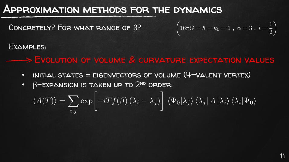
Evolution of volume & curvature expectation values

Approximation methods for the dynamics
Concretely? For what range of β?
Examples:
11
• initial states = eigenvectors of volume (4-valent vertex)
Evolution of volume & curvature expectation values
Approximation methods for the dynamics
Concretely? For what range of β?
Examples:
11
• initial states = eigenvectors of volume (4-valent vertex)
• β-expansion is taken up to 2nd
order:
Evolution of volume & curvature expectation values

Approximation methods for the dynamics
Concretely? For what range of β?
Examples:
11
• initial states = eigenvectors of volume (4-valent vertex)
• β-expansion is taken up to 2nd
order:
• time-expansion is taken up to 4th
order:
Evolution of volume & curvature expectation values

Approximation methods for the dynamics
Scalar field model in examples
12
j=2 j=10

Approximation methods for the dynamics
Scalar field model in examples
12
Periodic evolution at 0th
order
j=2 j=10

Approximation methods for the dynamics
Dust field model in examples
13
j=10j=10
Approximation methods for the dynamics
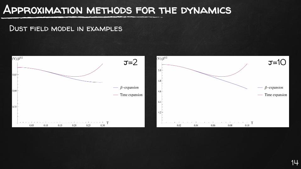
Dust field model in examples
14
j=10j=2

Summary & outlook

Summary & outlook
Deparametrized models:
Symmetric Hamiltonian operators
Approximation method (pert. th.) for the Hamiltonian op.:
* treatment of the square root in the SF model
* explicit computation of dynamics
Self-adjointness proofs
Identification & interpretation of relevant physical states
Include Standard Model