Approximation algorithms via randomized rounding: asurvey

Aravind Srinivasan∗

Abstract

Approximation algorithms provide a natural way to approach computationally hardproblems. There are currently many known paradigms in this area, including greedy al-gorithms, primal-dual methods, methods based on mathematical programming (linearand semidefinite programming in particular), local improvement, and “low distortion”embeddings of general metric spaces into special families of metric spaces. Random-ization is a useful ingredient in many of these approaches, and particularly so in theform of randomized rounding of a suitable relaxation of a given problem. We surveythis technique here, with a focus on correlation inequalities and their applications.

1 Introduction

It is well-known that several basic problems of discrete optimization are computationallyintractable (NP-hard or worse). However, such problems do need to be solved, and a veryuseful practical approach is to design a heuristic tailor-made for a particular application. An-other approach is to develop and implement approximation algorithms for the given problem,which come with proven guarantees. Study of the approximability of various classes of hard(combinatorial) optimization problems has greatly bloomed in the last two decades. In thissurvey, we study one important tool in this area, that of randomized rounding. We have notattempted to be encyclopaedic here, and sometimes do not present the best-known results;our goal is to present some of the underlying principles of randomized rounding withoutnecessarily going into full detail.

For our purposes here, we shall consider an algorithm to be efficient if it runs in polyno-mial time (time that is bounded by a fixed polynomial of the length of the input). We willnot explicitly present the running times of our algorithms; it will mostly be clear from thecontext that they are polynomial-time. However, we remark that most of our algorithms areindeed reasonably efficient; for instance, most of them involve network flows and other spe-cial cases of linear programming, for which efficient algorithms and codes are available. Our

∗Bell Laboratories, Lucent Technologies, Murray Hill, NJ 07974-0636, USA. This article was written whenthe author was with the School of Computing, National University of Singapore, Singapore 119260. Researchsupported in part by National University of Singapore Academic Research Fund Grant RP970607.

1

focus throughout will be on the quality of approximation guaranteed by our approximationalgorithms; we now recall the notion of an approximation algorithm.

Given an optimization problem P and an instance I of P , let OPT (I) denote the op-timal objective-function value for I; each feasible solution for I will have a non-negativeobjective-function value, for all problems P studied here. If P is a maximization problem,an approximation algorithmA for P is an efficient algorithm that, for some λ ≥ 1, produces afeasible solution of value at least OPT (I)/λ for all instances I. A is called a λ-approximationalgorithm for P ; λ is the approximation guarantee or approximation bound of A. To maintainthe convention that λ ≥ 1 for minimization problems also, we define an algorithm A to be aλ-approximation algorithm for a minimization problem P , if A produces a feasible solutionof value at most OPT (I) · λ for all instances I of P . For all problems considered, the goalwill be to to develop polynomial-time algorithms with improved (smaller) approximationguarantees.

Thus, the two key phrases in approximation algorithms are efficiency and proven approx-imation guarantees. As mentioned in the abstract, various paradigms have been developedin designing approximation algorithms; furthermore, beautiful connections between error-correcting codes, interactive proof systems, complexity classes and approximability havebeen established, showing that some basic problems (such as finding a maximum indepen-dent set in a given graph) are hard to approximate within any “reasonable” factor. From theviewpoint of computational complexity, an interesting observation that has resulted from thestudy of approximation algorithms is that though NP-complete problems are “equivalent”in the sense of exact solvability, their (“natural”) optimization versions turn out to lie ina wide spectrum in terms of approximability. The reader is referred to Hochbaum [32] fora comprehensive collection of articles discussing positive and negative results on approxi-mation algorithms; the chapter in it by Motwani, Naor & Raghavan discusses randomizedapproximation algorithms [55]. Also, the survey by Shmoys [65] is a good source for workon approximation algorithms via linear programming.

This survey will focus on one useful approach in designing approximation algorithms:randomized rounding. Recall the classical notion of a relaxation of an optimization problemP : given an instance I of P , we enlarge the set of feasible solutions for I in such a way thatthe objective function can be efficiently optimized over the enlarged set. Let x∗ denote an(efficiently computed) optimal solution over the enlarged set. Randomized rounding refersto the use of randomization to map x∗ back to a solution that is indeed feasible for I. Let y∗

denote the optimal objective function value on the enlarged set; i.e., the objective functionvalue at x∗. It is easily seen that y∗ ≥ OPT (I) (resp., y∗ ≤ OPT (I)) for maximization (resp.,minimization) problems P . Thus, suppose P is a maximization problem, say, and that wecan analyze our randomized rounding process to show that it results in a feasible solutionwith objective function value at least y∗/λ (in expectation or with high probability); thus,since y∗ ≥ OPT (I), the result is a λ-approximation (in expectation or with high probability).The situation is similar for minimization problems. Why the term “rounding”? One reasonis that the relaxation often involves relaxing integrality constraints on variables (such as“xi ∈ 0, 1”) to their real analogs (“xi ∈ [0, 1]”). Thus, potentially non-integral values will

2

have to be rounded to appropriate integers, by the randomized algorithm.Let us dive in by presenting two elegant examples of randomized rounding. Though these

do not lead to the currently best-known results, they demonstrate the power and elegance ofthe method. In the sequel, E[X] will denote the expected value of a random variable X, andPr[A] will denote the probability of event A. To appreciate our two examples, let us recall:(i) that if X is a random variable taking values in 0, 1, then E[X] = Pr[X = 1], (ii) thatthe uniform distribution on a finite set S places equal probability (1/|S|) on each element ofS; the uniform distribution on a finite real interval [a, b) has density function 1/(b− a), and(iii) linearity of expectation: for any finite number of arbitrary random variables X1, X2, . . .,E[∑iXi] =

∑i E[Xi].

(a) s− t cuts in graphs. This result is from Teo [73]. For some classical integer program-ming problems, it is known that they are well-characterized by a natural linear programmingformulation, i.e., that the linear and integral optima are the same. One famous example isthe following min-cut problem. Given an undirected graph G = (V,E) with a cost ci,j oneach edge i, j and two different distinguished vertices s and t, the problem is to remove aminimum-cost set of edges from G such that s gets disconnected from t. In other words, wewant a minimum-cost “cut” (partition of V into two sets) separating s and t.

Let us formulate the problem in a natural way as an integer linear program (ILP). Givena cut that separates s and t, let xi = 0 for all vertices i that are reachable from s, and xi = 1for all other vertices. (Thus, xs = 0 and xt = 1.) Let zi,j be the indicator variable for edgei, j crossing the cut; so zi,j = |xi − xj|. Thus, we have an integer program

minimize∑i,j∈E

ci,jzi,j subject to

∀i, j ∈ E, zi,j ≥ (xi − xj) and zi,j ≥ (xj − xi);xs = 0 and xt = 1; (1)

∀i ∀j, xi, zi,j ∈ 0, 1. (2)

It is easy to check that in any optimal solution to this integer program, we will have zi,j =|xi−xj|; hence, this is indeed a valid formulation. Now, suppose we relax (2) to ∀i∀j, xi, zi,j ∈[0, 1]. Thus, we get a linear program (LP) and as seen above, its optimal value y∗ is a lowerbound on the optimal objective function value OPT of the above integer program.

Now, it is well-known that in fact we have y∗ = OPT ; we now give a quick proof viarandomized rounding. Let

x∗i , z∗i,j ∈ [0, 1] : i, j ∈ V, i, j ∈ E

denote an optimal solution to the LP relaxation; once again, z∗i,j = |x∗i − x∗j | holds for alli, j ∈ E. Pick a u ∈ [0, 1) using the uniform distribution; for each i ∈ V , define xi := 0if x∗i ≤ u, and xi := 1 otherwise. This is our “randomized rounding” process here. Notethat constraint (1) is indeed satisfied by this method. What is the quality (cost) of the cut

3

produced? Fix any i, j ∈ E. This edge will cross the cut iff u ∈ [minx∗i , x∗j,maxx∗i , x∗j);this happens with probability |x∗j − x∗i |, i.e., z∗i,j. Thus, E[zi,j] = z∗i,j and hence by linearityof expectation,

E[∑i,j∈E

ci,jzi,j] =∑i,j∈E

ci,jE[zi,j] =∑i,j∈E

ci,jz∗i,j = y∗. (3)

The random variable∑i,j∈E ci,jzi,j is piecewise continuous as a function of u (with only

finitely many break-points). So, by (3), there must be some value of u that leads to anintegral solution of cost no more than y∗! Thus y∗ = OPT . See Teo & Sethuraman [74] forapplications of more sophisticated versions of this idea to the stable matching problem.

(b) Maximum satisfiability (MAX-SAT). This is a natural optimization version ofthe satisfiability problem. Given a Boolean formula F in conjunctive normal form and anon-negative weight wi associated with each clause Ci, the objective is to find a Booleanassignment to the variables that maximizes the total weight of the satisfied clauses. Thisproblem is clearly NP-hard. An approximation algorithm that always produces a solutionof weight at least 3/4th of the optimal weight OPT , had been proposed by Yannakakis [77];we now describe a simpler algorithm of Goemans & Williamson that matches this [27].

The idea is to consider two different randomized schemes for constructing the Booleanassignment, and observe that they have complementary strengths in terms of their approx-imation guarantees. The first works well when each clause has “several” literals, while thesecond will be good if each clause has “few” literals. Thus, we could run both and take thebetter solution; in particular, we could choose one of the two schemes uniformly at random,and the resulting solution’s objective function value will be the arithmetic mean of the re-spective solutions of the two schemes. Let us now present these simple schemes and analyzethem.

The first scheme is to set each variable uniformly at random to True or False, independentof the other variables. Let |Ci| denote the length of (i.e., number of literals in) clause Ci. Itis easy to check that

pi,1 = Pr[Ci satisfied] = 1− 2−|Ci|; (4)

hence, this scheme works well if all clauses are “long”.However, it is intuitively clear that such an approach may not work well for all CNF

formulae: those with most clauses being short, in particular. Our second scheme is to startwith a (fairly obvious) integer programming formulation. For each clause Ci, let P (i) denotethe set of unnegated variables appearing in it, and N(i) be the set of negated variables init. For each variable j, let xj = 1 if this variable is set to True, and xj = 0 if the variable isset to False. Letting zi ∈ 0, 1 be the indicator for clause Ci getting satisfied, we have theconstraint

∀i, zi ≤ (∑

j∈P (i)

xj) + (∑

j∈N(i)

(1− xj)). (5)

Subject to these constraints, the objective is to maximize∑iwizi. It is easy to check that

this is a correct formulation for the problem on hand.

4

As above, suppose we take the LP relaxation obtained by relaxing each xj and zi to bea real in [0, 1], subject to (5). Then, y∗ is an upper bound on OPT . Let x∗j , z∗i be thevalues of the variables in an optimal solution to the LP. The key is to interpret each x∗j asa probability [58]. Thus, our randomized rounding process will be, independently for each j,to set xj := 1 (i.e., make variable j True) with probability x∗j and xj := 0 (make variable jFalse) with probability 1 − x∗j . One intuitive justification for this is that if x∗j were “high”,i.e., close to 1, it may be taken as an indication by the LP that it is better to set variable jto True; similarly for the case where xj is close to 0. This is our second rounding scheme;since we are using information provided by the LP optimum implicitly, the hope is that wemay be using the given formula’s structure better in comparison with our first scheme.

Let us lower-bound the probability of clause Ci getting satisfied. We can assume withoutloss of generality that all variables appear unnegated in Ci. Thus, by (5), we will have

z∗i = min∑

j∈P (i)

x∗j , 1.

Given this, it is not hard to check that Pr[Ci satisfied] = 1 − ∏j∈P (i)(1 − x∗j) is minimizedwhen each x∗j equals z∗i /|Ci|. Thus,

pi,2 = Pr[Ci satisfied] ≥ 1− (1− z∗i /|Ci|)|Ci|. (6)

For a fixed value of z∗i , the term 1−(1−z∗i /|Ci|)|Ci| decreases monotonically as |Ci| increases.This is the sense in which our two schemes are complementary.

So, as mentioned above, suppose we choose one of the two schemes uniformly at random,in order to balance their strengths. Then,

Pr[Ci satisfied] = (pi,1 + pi,2)/2

≥ 1− (2−|Ci| + (1− z∗i /|Ci|)|Ci|)/2≥ (3/4)z∗i ,

via elementary calculus and the fact that z∗i ∈ [0, 1]. (For any fixed positive integer `,f(`, x) = 1− (2−` + (1− x/`)`)/2− 3x/4 has a non-positive derivative for x ∈ [0, 1]. Thus,it suffices to show that f(`, 1) ≥ 0 for all positive integers `. We have f(1, 1) = f(2, 1) = 0.For ` ≥ 3, 2−` ≤ 1/8 and (1 − 1/`)` ≤ 1/e; so f(`, 1) ≥ 0 for ` ≥ 3.) So by linearity ofexpectation, the expected weight of the final Boolean assignment is at least

∑i(3/4)wiz

∗i =

(3/4)y∗ ≥ (3/4)OPT . Thus, at least in expectation, the assignment produced has a goodapproximation ratio; this randomized algorithm can be “derandomized” (turned into anefficient deterministic algorithm) as shown in [27].

Can this analysis be improved? No; we cannot guarantee any bound larger than (3/4)y∗.To see this, consider, e.g., the situation where we have two variables x1 and x2, all 4 clausesthat can be formed using both variables, and with all the wi being 1. It is easy to see thaty∗ = 4 and OPT = 3 here. Thus, there are indeed situations where OPT = (3/4)y∗. Thisalso shows a simple approach to decide if a certain relaxation-based method is best possible

5

using that particular relaxation: to show that there are situations where the gap betweenthe relaxed optimum and the optimum is (essentially) as high as the approximation boundguaranteed for that method. The worst-case ratio between the fractional and integral optimais called the integrality gap: clearly, a straightforward LP-based method cannot guaranteean approximation ratio better than the integrality gap.

In the s−t cut example, we saw an instance of dependent randomized rounding: no two xiare independent. In contrast, the underlying random choices were made independently in theMAX-SAT example; this is the basic approach we will focus on for most of this survey. Thegeneral situation here is that for some “large” N , we must choose, for i = 1, 2, . . . , N , xi froma finite set Si (in order to optimize some function of the xi, subject to some constraints on thechoices). The randomized rounding approach will be to choose each xi independently fromSi, according to some distribution Di. This approach can be broadly classified as follows.First, as in our first scheme in the MAX-SAT example, we could take the arguably simplestapproach–in this context–of letting each Di be the uniform distribution on Si; we call thisuniform randomized rounding. This approach, while most natural for some problems, is ingeneral inferior to choosing all the Di through linear programming (as in the second schemeabove in the MAX-SAT example), which we term LP-based randomized rounding.

The rest of this survey is organized as follows. We begin with some preliminaries inSection 2. In Section 3, we study approximation algorithms for packet-routing and job-shopscheduling that use uniform randomized rounding. Sections 4, 5 and 6 then consider LP-based randomized rounding. In Section 4, we show how a useful correlation inequality, theFKG inequality, can be applied to derive improved approximation algorithms for a class ofrouting, packing and covering problems. Section 5 considers a family of situations wherecorrelations complementary to those handled by the FKG inequality arise. In Section 6, westudy applications of a recent extension of the Lovasz Local Lemma. Section 7 sketches howmany such rounding problems are instances of questions in discrepancy theory, and brieflydescribes some seminal work of Beck & Fiala, Beck, Spencer and Banaszczyk in this area. Abrief sketch of some other relaxation methods and open questions are presented in Section8, which concludes.

Due to the immense current interest in communication networks and routing algorithms,many optimization problems we consider will be based on routing and scheduling. Two otherbasic themes of much of this survey are: (a) the use of various correlation inequalities inanalyzing randomized rounding processes, and (b) their applications for ILPs with column-sparse coefficient matrices in particular. (Roughly speaking, a matrix A is column-sparse ifwe can bound the maximum number of nonzero entries in, or the L1 norm of, any columnof A by an appropriate parameter.)

2 Preliminaries

Let “r.v.” denote the phrase “random variable”; we will be concerned only with discrete-valued r.v.s here. Given a non-negative integer k, [k] will denote the set 1, 2, . . . , k; loga-rithms are to the base two unless specified otherwise. Let Z+ denote the set of non-negative

6

integers. Given an event E , its indicator random variable χ(E) is defined to be 1 if E holds,and 0 otherwise. Note that E[χ(E)] = Pr[E ].

Informally, a randomized algorithm is an algorithm equipped with a random numbergenerator that can output any desired number of unbiased (fair) and, more importantly,independent random bits. The algorithm requests any number of random bits needed forits computation, from the source; we may charge, e.g., unit time to get one random bit.As seen in the introduction, it is also convenient to be able to draw an r.v. that is uni-formly distributed over some finite real interval [a, b) or some finite set; we shall assume thatour random source has such features also, when necessary. The “random bits” model cantypically approximate these requirements with sufficient accuracy in the context of efficientrandomized algorithms.

There are several advantages offered by randomness to computation. See the books ofAlon, Spencer & Erdos [4] and Motwani & Raghavan [56] for various aspects and applicationsof randomized computation.

2.1 Large deviation bounds

We now present a basic class of results which are often needed in randomized computation.These are (upper) bounds on the probability of certain types of r.v.s deviating significantlyfrom their mean, and hence are known as large deviation or tail probability bounds. We shallpresent just a few of these results here that are relevant to randomized algorithms.

For the rest of this subsection, we let µ denote E[X] for a random variable X. One ofthe most basic tail inequalities is Markov’s inequality, whose proof is left as an exercise.

Lemma 2.1 (Markov’s inequality) If an r.v. X takes on only non-negative values, thenfor any a > 0, Pr[X ≥ a] ≤ µ/a.

Markov’s inequality is best-possible if no further information is given about the r.v. X.However, it is often too weak, e.g., when we wish to upper bound the lower tail probability,or probability of staying much below the mean, of an r.v. X, even if we know good upper andlower bounds on the extent of its support. More information about the r.v. X of interest canlead to substantially stronger bounds, as we shall soon see. Nevertheless, Markov’s inequalitystill underlies the approach behind many of these bounds. A well-known such strengtheningof Markov’s inequality is Chebyshev’s inequality, which can be applied if we can upper boundthe variance of X, E[(X − µ)2], well. Recall that the positive square root of the variance ofX is known as the standard deviation of X.

Lemma 2.2 (Chebyshev’s inequality) For any r.v. X and any a > 0, Pr[|X−µ| ≥ a] ≤σ2/a2, where σ denotes the standard deviation of X.

If X is a sum of independent r.v.s, each of which lies in [0, 1], then it is not hard to verifythat E[(X − µ)2] ≤ E[X]. Thus we get

Corollary 2.1 Let X be a sum of independent r.v.s, each of which lies in [0, 1]. Then, forany a > 0, Pr[|X − µ| ≥ a] ≤ µ/a2.

7

Hence, r.v.s X with a small standard deviation have good tail behavior. But this can bestrengthened much more, for a class of r.v.s X that occur often in randomized computation:sums of independent r.v.s Xi, where each Xi ∈ [0, 1]. The idea here is to observe that

Pr[X ≥ a] = Pr[etX ≥ eta] ≤ E[etX ]/eta

for any t > 0, where the last step follows from Markov’s inequality. We may then (ap-proximately) minimize the last ratio over t > 0, to get strong bounds. Note also that thisapproach holds for any r.v. X, not just for sums of independent random variables. Similarly,for a < µ, we can upper bound Pr[X ≤ a] by mint>0 E[e−tX ]/e−ta.

Let X1, X2, . . . Xn be independent r.v.s that take on values in [0, 1], with E[Xi] = pi,1 ≤ i ≤ n. Let X

.=∑ni=1 Xi, and µ

.= E[X] =

∑ni=1 pi. We want good upper bounds on

Pr[X ≥ µ(1 + δ)], for δ > 0; we recall some such bounds now, as presented in [61]. Chernoff[18] showed that for identically distributed 0, 1 r.v.s X1, X2, . . . , Xn and for a > µ,

mint

E[etX ]

eat≤ Λ(n, µ, a) = (

µ

a)a(

n− µn− a

)n−a.

Hoeffding [33] extended this by showing that Λ(n, µ, a) is an upper bound for the aboveminimum even if the Xi’s are not identically distributed and range between 0 and 1. Re-placing a with µ(1 + δ) in the Hoeffding estimate Λ(·, ·, ·) gives, for δ ≥ 0,

Pr[X ≥ µ(1 + δ)] ≤ F (n, µ, δ).=

(1 + µδ(n−µ(1+δ))

)n−µ(1+δ)

(1 + δ)µ(1+δ). (7)

For δ ∈ [0, 1], Hoeffding’s approach also gives

Pr[X ≤ µ(1− δ)] = Pr[n−X ≥ n− µ(1− δ)] ≤ F (n, µ,−δ) .=

(1− µδ(n−µ(1−δ)))

n−µ(1−δ)

(1− δ)µ(1−δ) . (8)

The following related results are useful (see, e.g., [33, 5, 4, 56]).

If δ ≥ 0, Pr[X ≥ µ(1 + δ)] ≤∏i∈[n] E[(1 + δ)Xi ]

(1 + δ)µ(1+δ)≤ G(µ, δ)

.=

(eδ

(1 + δ)(1+δ)

)µ; (9)

If δ ∈ [0, 1], Pr[X ≤ µ(1− δ)] ≤∏i∈[n] E[(1− δ)Xi ](1− δ)µ(1−δ) ≤ H(µ, δ)

.= e−µδ

2/2. (10)

It can be checked that for δ ≤ 1, G(µ, δ) ≤ e−δ2µ/3; for δ > 1, G(µ, δ) ≤ e−(1+δ) ln(1+δ)µ/4.

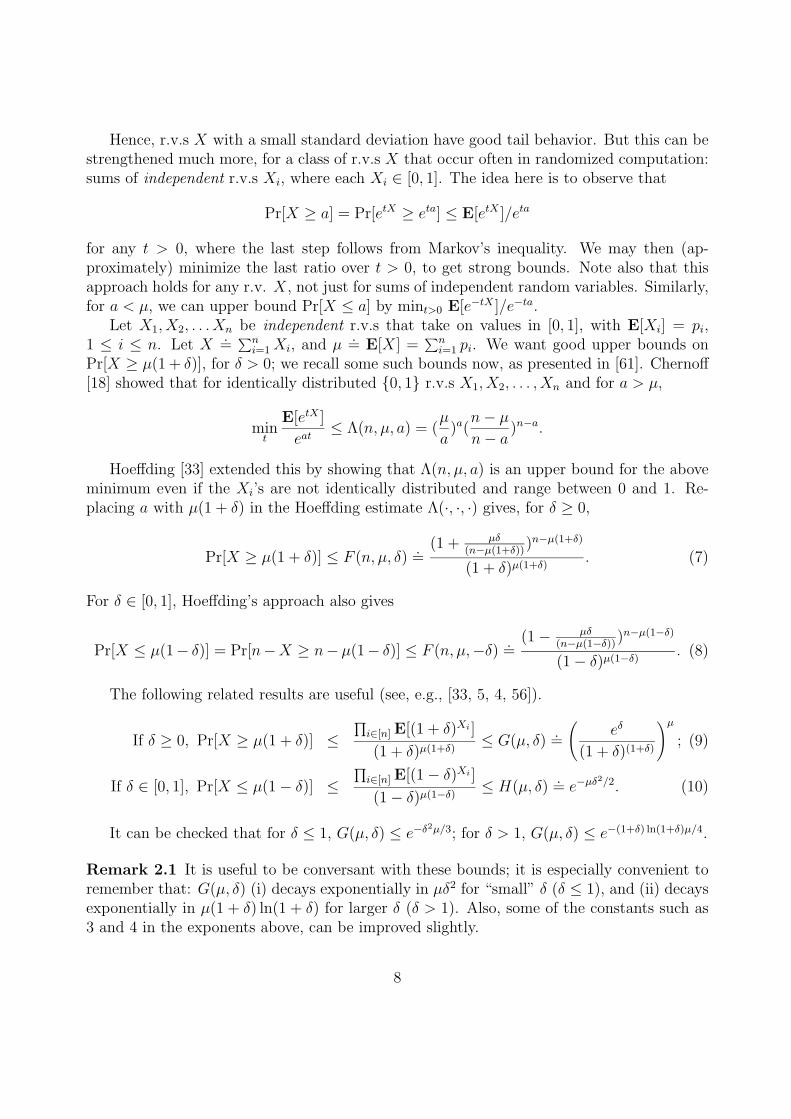
Remark 2.1 It is useful to be conversant with these bounds; it is especially convenient toremember that: G(µ, δ) (i) decays exponentially in µδ2 for “small” δ (δ ≤ 1), and (ii) decaysexponentially in µ(1 + δ) ln(1 + δ) for larger δ (δ > 1). Also, some of the constants such as3 and 4 in the exponents above, can be improved slightly.

8

We next present a useful result from [61], which offers a new look at the Chernoff-

Hoeffding (CH) bounds. For real x and any positive integer r, let(xr

) .= x(x−1)···(x−r+1)

r!as

usual, with(x0

) .= 1. Define, for z = (z1, z2, . . . , zn) ∈ <n, a family of symmetric polynomials

ψj(z), j = 0, 1, . . . , n, where ψ0(z) ≡ 1, and for 1 ≤ j ≤ n,

ψj(z).=

∑1≤i1<i2···<ij≤n

zi1zi2 · · · zij .

A small extension of a result of [61] is:

Theorem 2.1 ([61]) Given r.v.s X1, . . . , Xn ∈ [0, 1], let X =∑ni=1 Xi and µ = E[X]. (a)

For any δ > 0, any nonempty event Z and any k ≤ µ(1 + δ), Pr[X ≥ µ(1 + δ)|Z] ≤ E[Yk|Z],

where Yk = ψk(X1, . . . , Xn)/(µ(1+δ)k

). (b) If the Xis are independent and k = dµδe, then

Pr[X ≥ µ(1 + δ)] ≤ E[Yk] ≤ G(µ, δ).

Proof: Suppose b1, b2, . . . bn ∈ [0, 1] satisfy∑ni=1 bi ≥ a. It is not hard to show that for

any non-negative integer k ≤ a, ψk(b1, b2, . . . , bn) ≥(ak

). (This is immediate if each bi lies in

0, 1, and takes a little more work if bi ∈ [0, 1].) Now this holds even conditional on anypositive probability event Z. Hence,

Pr[X ≥ µ(1 + δ)|Z] ≤ Pr[Yk ≥ 1|Z] ≤ E[Yk|Z],

where the second inequality follows from Markov’s inequality. See [61] for a proof of (b).

3 Uniform randomized rounding

We start our discussion in Section 3.1 with a basic random process that is related to manysituations in uniform randomized rounding. More sophisticated versions of this process arethen used in Section 3.2 to present approximation algorithms for job-shop scheduling, andin Section 3.4 for a version of packet routing (which is an important special case of job-shopscheduling).

3.1 Simple balls-and-bins processes

Consider the situation where each of n given balls is thrown uniformly at random, indepen-dently, into one of n bins. (We can view this as throwing darts at random.) Let X denotethe maximum number of balls in any bin. It is often useful to know facts about (or boundson) various statistics of X. For instance, it is known that E[X] = (1 + o(1)) lnn/ ln lnn,where the o(1) term goes to 0 as n → ∞. Here, we content ourselves with showing that Xis not much above this expectation, with high probability.

Let Yi,j be the indicator random variable for ball i being thrown into bin j. Then, therandom variable Xj that denotes the number of balls in bin j, equals

∑i Yi,j. (We have

9

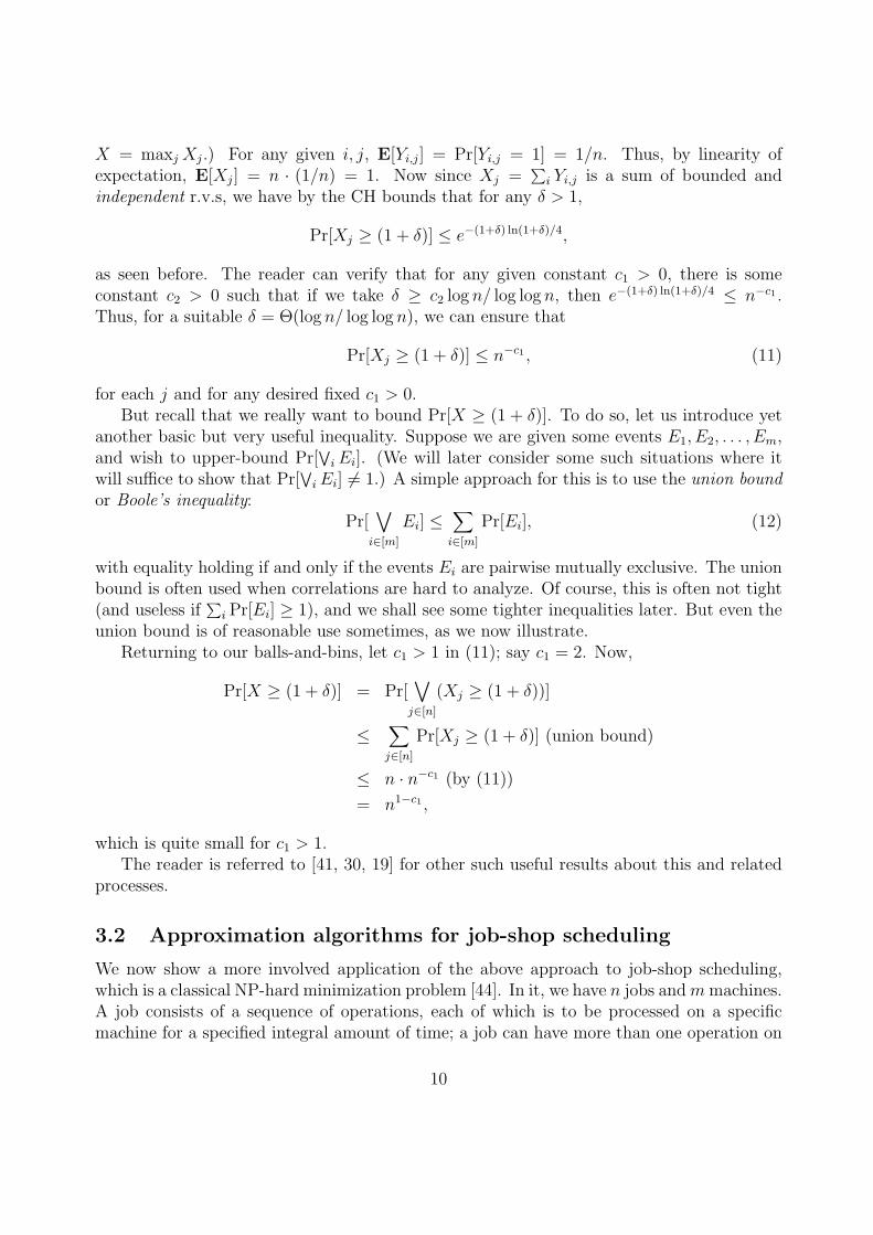
X = maxj Xj.) For any given i, j, E[Yi,j] = Pr[Yi,j = 1] = 1/n. Thus, by linearity ofexpectation, E[Xj] = n · (1/n) = 1. Now since Xj =

∑i Yi,j is a sum of bounded and

independent r.v.s, we have by the CH bounds that for any δ > 1,

Pr[Xj ≥ (1 + δ)] ≤ e−(1+δ) ln(1+δ)/4,

as seen before. The reader can verify that for any given constant c1 > 0, there is someconstant c2 > 0 such that if we take δ ≥ c2 log n/ log log n, then e−(1+δ) ln(1+δ)/4 ≤ n−c1 .Thus, for a suitable δ = Θ(log n/ log log n), we can ensure that

Pr[Xj ≥ (1 + δ)] ≤ n−c1 , (11)

for each j and for any desired fixed c1 > 0.But recall that we really want to bound Pr[X ≥ (1 + δ)]. To do so, let us introduce yet

another basic but very useful inequality. Suppose we are given some events E1, E2, . . . , Em,and wish to upper-bound Pr[

∨iEi]. (We will later consider some such situations where it

will suffice to show that Pr[∨iEi] 6= 1.) A simple approach for this is to use the union bound

or Boole’s inequality:Pr[

∨i∈[m]

Ei] ≤∑i∈[m]

Pr[Ei], (12)

with equality holding if and only if the events Ei are pairwise mutually exclusive. The unionbound is often used when correlations are hard to analyze. Of course, this is often not tight(and useless if

∑i Pr[Ei] ≥ 1), and we shall see some tighter inequalities later. But even the

union bound is of reasonable use sometimes, as we now illustrate.Returning to our balls-and-bins, let c1 > 1 in (11); say c1 = 2. Now,

Pr[X ≥ (1 + δ)] = Pr[∨j∈[n]

(Xj ≥ (1 + δ))]

≤∑j∈[n]

Pr[Xj ≥ (1 + δ)] (union bound)

≤ n · n−c1 (by (11))

= n1−c1 ,

which is quite small for c1 > 1.The reader is referred to [41, 30, 19] for other such useful results about this and related

processes.

3.2 Approximation algorithms for job-shop scheduling

We now show a more involved application of the above approach to job-shop scheduling,which is a classical NP-hard minimization problem [44]. In it, we have n jobs andmmachines.A job consists of a sequence of operations, each of which is to be processed on a specificmachine for a specified integral amount of time; a job can have more than one operation on

10

a given machine. The operations of a job must be processed in the given sequence, and amachine can process at most one operation at any given time. The problem is to schedulethe jobs so that the makespan, the time when all jobs have been completed, is minimized.An important special case is preemptive scheduling, wherein machines can suspend work onoperations, switch to other operations, and later resume the suspended operations; this isoften reasonable, for instance, in scheduling jobs in operating systems. Note that in thepreemptive setting, all operation lengths may be taken to be one. If pre-emption is notallowed, we have the hard non-preemptive case, which we study here.

More formally, a job-shop scheduling instance consists of jobs J1, J2, . . . , Jn, machinesM1,M2, . . . , Mm, and for each job Jj, a sequence of `j operations (Mj,1, tj,1), (Mj,2, tj,2), . . . ,(Mj,`j , tj,`j). Each operation is a (machine, processing time) pair: each Mj,k represents somemachine Mi, and the pair (Mj,i, tj,i) signifies that the corresponding operation of job Jj mustbe processed on machine Mj,i for an uninterrupted integral amount of time tj,i. A machinecan process at most one operation at any time, and the operations of each job must beprocessed in the given order.

Even some very restricted special cases of job-shop scheduling are NP-hard. Furthermore,while the theory of NP-completeness shows all NP-complete problems to be “equivalent”in a sense, NP-optimization problems display a wide range of difficulty in terms of exactsolvability in practice; some of the hardest such problems come from job-shop scheduling.Define a job-shop instance to be acyclic if no job has two or more operations that need torun on any given machine. A single instance of acyclic job-shop scheduling with 10 jobs,10 machines and 100 operations resisted attempts at exact solution for 22 years until itsresolution [17]. See also Applegate & Cook [6]. We will show here that good approximationalgorithms do exist for job-shop scheduling.

There are two natural lower bounds on the makespan of any job-shop instance: Pmax, themaximum total processing time needed for any job, and Πmax, the maximum total amountof time for which any machine has to process operations. For the NP-hard special case ofacyclic job-shop scheduling wherein all operations have unit length, the amazing result thata schedule of makespan O(Pmax + Πmax) always exists, was shown in [46]. (We shall sketchthe approach of [46] in Section 3.4.) Such a schedule can also be computed in polynomialtime [47]. Can such good bounds hold if we drop any one of the two assumptions of acyclicityand unit operation lengths? See [23] for some recent advances on questions such as this.

Returning to general job-shop scheduling, let µ = maxj `j denote the maximum numberof operations per job, and let pmax be the maximum processing time of any operation. Byinvoking ideas from [46, 62, 63] and by introducing some new techniques, good approximationalgorithms were developed in [66]; their deterministic approximation bounds were slightlyimproved in [61]. (Recall that an approximation algorithm is an efficient algorithm thatalways produces a feasible solution that is to within a certain guaranteed factor of optimal.)

Theorem 3.1 ([66, 61]) There is a deterministic polynomial-time algorithm that delivers

a schedule of makespan O((Pmax +Πmax) · log(mµ)log log(mµ)

· log(minmµ, pmax)) for general job-shopscheduling.

11

This has been improved further in [29]; we just discuss some of the main ideas behindTheorem 3.1 now. A key ingredient here is a “random delays” technique due to [46], andits intuition is as follows. To have a tractable analysis, suppose we imagine for now thateach job Jj is run continuously after an initial wait of dj steps: we wish to pick a suitabledelay dj from Sj = 0, 1, . . . , B − 1 for an appropriate B, in such a way that the resulting“contentions” on machines is kept hopefully low. It seems a reasonable idea to conductuniform randomized rounding, i.e., to pick each dj uniformly and independently at randomfrom 0, 1, . . . , B − 1. In a manner similar to our dart-throwing analysis, we will thenargue that, with high probability, not too many jobs contend for any given machine at thesame time. We then resolve contentions by “expanding” the above “schedule”; the “lowcontention” property is invoked to argue that a small amount of such expansion suffices.

Let us proceed more formally now. A delayed schedule of a job-shop instance is con-structed as follows. Each job Jj is assigned a delay dj in 0, 1, . . . ,Πmax − 1. In theresulting “schedule”, the operations of Jj are scheduled consecutively, starting at time dj.Recall that all operation lengths are integral. For a delayed schedule S, the contentionC(Mi, t) is defined to be the number of operations scheduled on machine Mi in the timeinterval [t, t+ 1). A randomly delayed schedule is a delayed schedule wherein the delays arechosen independently and uniformly at random from 0, 1, . . . ,Πmax − 1.

Remark 3.1 Recall that pmax denotes the maximum processing time of any operation. Itis shown in [66] that, in deterministic polynomial time, we can reduce the general shop-scheduling problem to the case where (i) pmax ≤ nµ, and where (ii) n ≤ poly(m,µ), whileincurring an additive O(Pmax + Πmax) term in the makespan of the schedule produced. Byconducting these reductions, we assume from now on that pmax and n are bounded bypoly(m,µ).

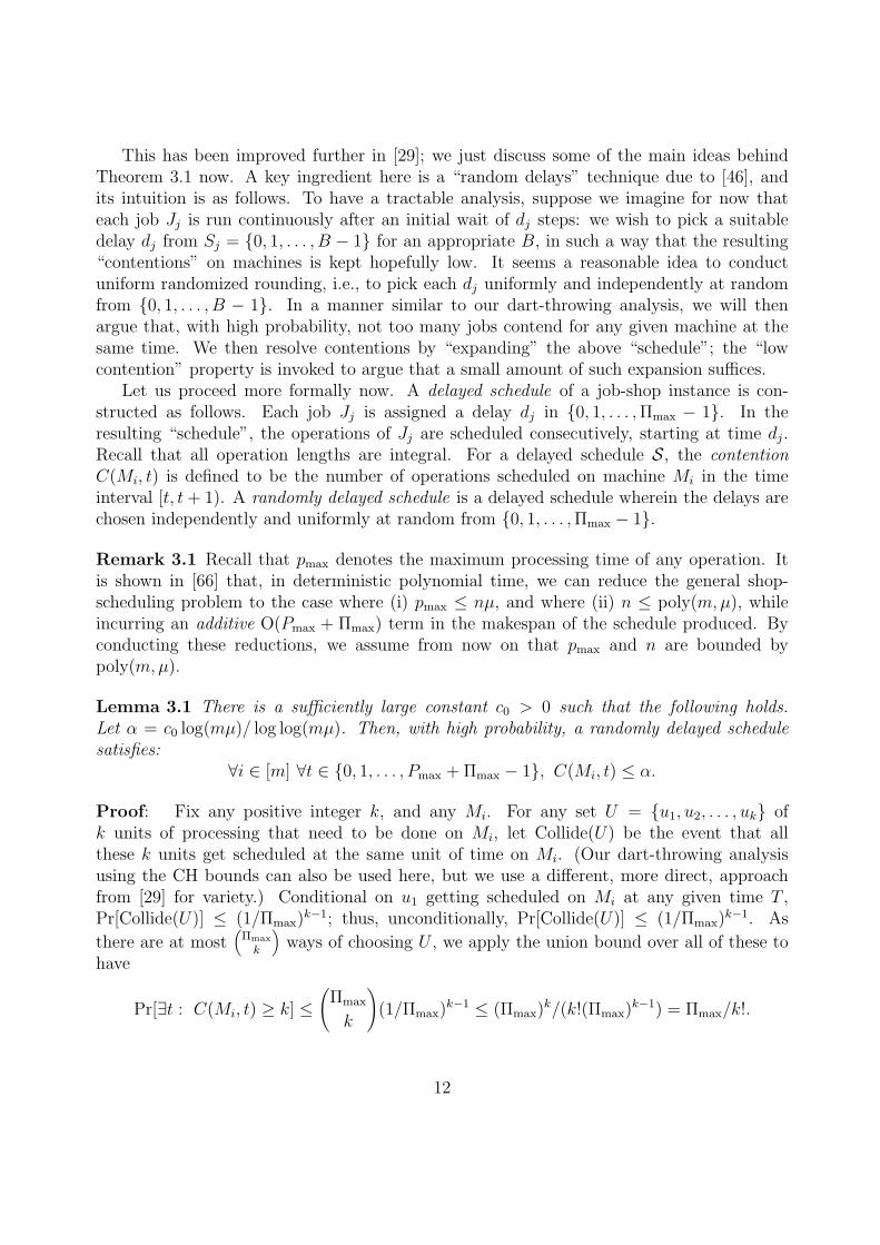
Lemma 3.1 There is a sufficiently large constant c0 > 0 such that the following holds.Let α = c0 log(mµ)/ log log(mµ). Then, with high probability, a randomly delayed schedulesatisfies:

∀i ∈ [m] ∀t ∈ 0, 1, . . . , Pmax + Πmax − 1, C(Mi, t) ≤ α.

Proof: Fix any positive integer k, and any Mi. For any set U = u1, u2, . . . , uk ofk units of processing that need to be done on Mi, let Collide(U) be the event that allthese k units get scheduled at the same unit of time on Mi. (Our dart-throwing analysisusing the CH bounds can also be used here, but we use a different, more direct, approachfrom [29] for variety.) Conditional on u1 getting scheduled on Mi at any given time T ,Pr[Collide(U)] ≤ (1/Πmax)k−1; thus, unconditionally, Pr[Collide(U)] ≤ (1/Πmax)k−1. As

there are at most(

Πmax

k

)ways of choosing U , we apply the union bound over all of these to

have

Pr[∃t : C(Mi, t) ≥ k] ≤(

Πmax

k

)(1/Πmax)k−1 ≤ (Πmax)k/(k!(Πmax)k−1) = Πmax/k!.

12

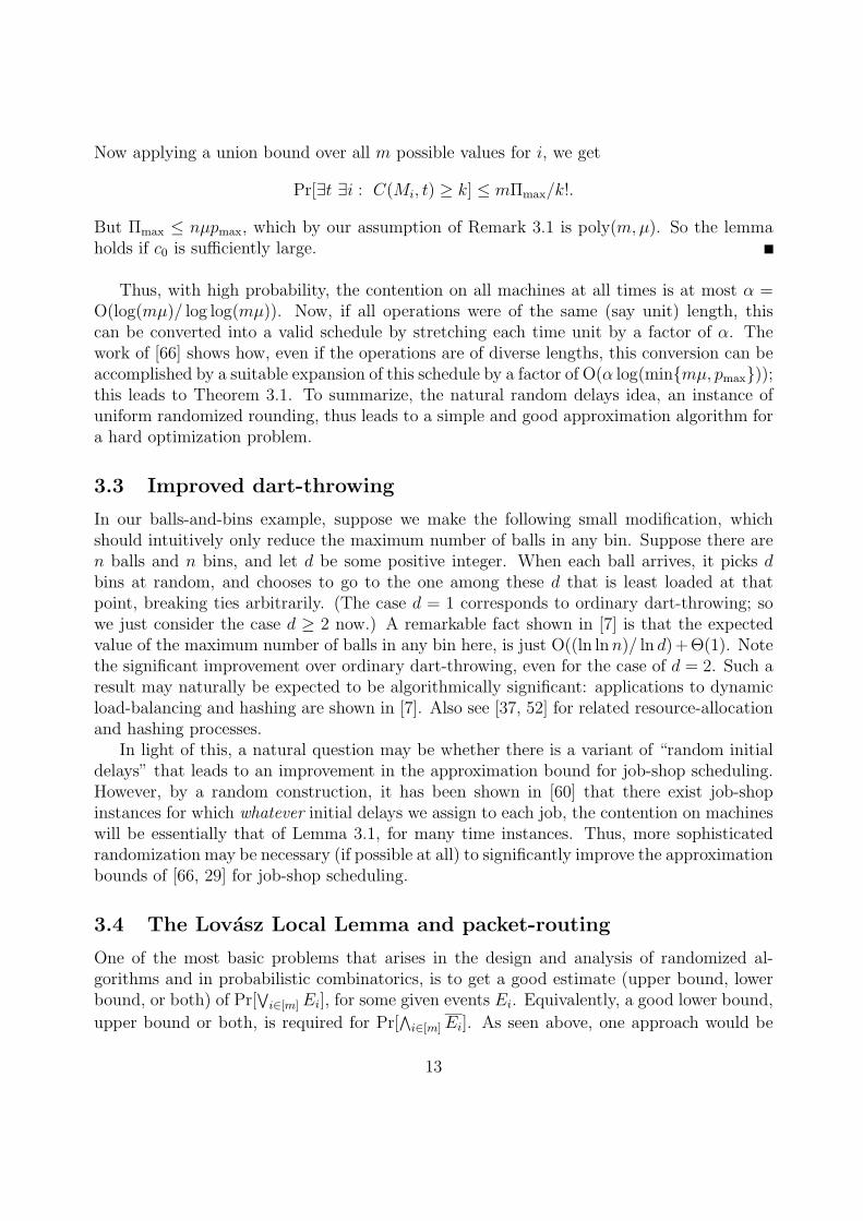
Now applying a union bound over all m possible values for i, we get

Pr[∃t ∃i : C(Mi, t) ≥ k] ≤ mΠmax/k!.

But Πmax ≤ nµpmax, which by our assumption of Remark 3.1 is poly(m,µ). So the lemmaholds if c0 is sufficiently large.

Thus, with high probability, the contention on all machines at all times is at most α =O(log(mµ)/ log log(mµ)). Now, if all operations were of the same (say unit) length, thiscan be converted into a valid schedule by stretching each time unit by a factor of α. Thework of [66] shows how, even if the operations are of diverse lengths, this conversion can beaccomplished by a suitable expansion of this schedule by a factor of O(α log(minmµ, pmax));this leads to Theorem 3.1. To summarize, the natural random delays idea, an instance ofuniform randomized rounding, thus leads to a simple and good approximation algorithm fora hard optimization problem.

3.3 Improved dart-throwing

In our balls-and-bins example, suppose we make the following small modification, whichshould intuitively only reduce the maximum number of balls in any bin. Suppose there aren balls and n bins, and let d be some positive integer. When each ball arrives, it picks dbins at random, and chooses to go to the one among these d that is least loaded at thatpoint, breaking ties arbitrarily. (The case d = 1 corresponds to ordinary dart-throwing; sowe just consider the case d ≥ 2 now.) A remarkable fact shown in [7] is that the expectedvalue of the maximum number of balls in any bin here, is just O((ln lnn)/ ln d) + Θ(1). Notethe significant improvement over ordinary dart-throwing, even for the case of d = 2. Such aresult may naturally be expected to be algorithmically significant: applications to dynamicload-balancing and hashing are shown in [7]. Also see [37, 52] for related resource-allocationand hashing processes.

In light of this, a natural question may be whether there is a variant of “random initialdelays” that leads to an improvement in the approximation bound for job-shop scheduling.However, by a random construction, it has been shown in [60] that there exist job-shopinstances for which whatever initial delays we assign to each job, the contention on machineswill be essentially that of Lemma 3.1, for many time instances. Thus, more sophisticatedrandomization may be necessary (if possible at all) to significantly improve the approximationbounds of [66, 29] for job-shop scheduling.

3.4 The Lovasz Local Lemma and packet-routing

One of the most basic problems that arises in the design and analysis of randomized al-gorithms and in probabilistic combinatorics, is to get a good estimate (upper bound, lowerbound, or both) of Pr[

∨i∈[m] Ei], for some given events Ei. Equivalently, a good lower bound,

upper bound or both, is required for Pr[∧i∈[m] Ei]. As seen above, one approach would be

13

to use the union bound (12) which is unfortunately quite weak in general. Another obviousapproach, which works when the events Ei are independent, is to use

Pr[∧i∈[m]

Ei] =∏i∈[m]

Pr[Ei],

the “independence sieve”.A common situation where we have to look for such bounds is when the events Ei are

“bad” events, all of which we wish to avoid simultaneously. The minimal requirement forthis is that Pr[

∧i∈[m] Ei] > 0; however, even to prove this, the independence sieve will often

not apply and the counting sieve could be quite weak. However, the independence sievedoes suggest something: can we say something interesting if each Ei is independent of mostother Ej? Let e denote the base of natural logarithms as usual. The powerful Lovasz LocalLemma (LLL) due to Erdos and Lovasz ([20]) is often very useful in such cases; see Chapter5 of [4] for many such applications. The LLL (symmetric case) shows that all of a set ofevents Ei can be avoided under some conditions:

Lemma 3.2 ([20]) Let E1, E2, . . . , Em be any events with Pr[Ei] ≤ p ∀i. If each Ei ismutually independent of all but at most d of the other events Ej and if ep(d+ 1) ≤ 1, then

Pr[m∧i=1

Ei] ≥ (1− ep)m > 0.

Why is the LLL considered such a powerful tool? For the union bound to be useful, wesee from (12) that Pr[Ei], averaged over all i, must be less than 1/m, which can be quitesmall if m is “large”. In contrast, the LLL shows that even maxi Pr[Ei] can be as high as(e(d + 1))−1, which is substantially bigger than 1/m if d m (say, if d = O(polylog(m))).Thus, under the “locality” assumption that d m, we can get away with maxi Pr[Ei] beingmuch bigger than 1/m. There is also a generalized (“asymmetric”) form of the LLL. See [4]for this and related points.

We now present a portion of a surprising result on routing due to Leighton, Maggs & Rao,which makes involved use of the LLL in conjunction with uniform randomized rounding [46].Suppose we have a routing problem on a graph, where the paths also have been specified foreach of the packets. Concretely, we are given an undirected graph G, a set of pairs of vertices(si, ti), and a path Pi in G that connects si with ti, for each i. Initially, we have one packetresiding at each si; this packet has to be routed to ti using the path Pi. We assume thata packet takes unit time to traverse each edge, and the main constraint as usual is that anedge can carry at most one packet per (synchronous) time step. Subject to these restrictions,we want to minimize the maximum time taken by any packet to reach its destination. (Ifwe view each edge as a machine and each packet as a job, this is just a special case of thejob-shop scheduling problem considered in Section 3.2. We may further assume that thepaths Pi are all edge-simple, i.e., do not repeat any edge; thus, we have an acyclic job-shopproblem, in the notation of Section 3.2. Our objective here also is to keep the makespansmall.) Since we are also given the paths Pi, the only question is the queuing discipline we

14

need to provide at the vertices (what a node must do if several packets that are currentlyresident at it, want to traverse the same edge on their next hop).

One motivation for assuming such a model (wherein the paths Pi are prespecified) isthat many routing strategies can be divided into two phases: (a) choosing an intermediatedestination for each packet (e.g., the paradigm of choosing the intermediate destination ran-domly and independently for each packet [75, 76]) and taking each packet on some canonicalpath to the intermediate destination, and (b) routing each packet on a canonical path fromthe intermediate destination to the final destination ti. Such a strategy can thus use twoinvocations of the above “prespecified paths” model. Section 7 contains a brief descriptionof recent work of [72] concerning situations where the paths Pi are not prespecified.

Let us study the objective function, i.e., the maximum time taken by any packet to reachits destination. Two relevant parameters are the congestion c, the maximum number of pathsPi that use any given edge in G, and the dilation d, the length of a longest path among thePi. It is immediate that each of c and d is a lower bound on the objective function. (Thecongestion and dilation are the respective analogs of Πmax and Pmax here.) In terms of upperbounds, the simple greedy algorithm that never lets an edge go idle if it can carry a packetat a given time step, terminates within cd steps; this is because any packet can be delayedby at most c− 1 other packets at any edge in the network.

Can we do better than cd? Recall our assumption that the paths Pi are all edge-simple.Under this assumption, the work of [46] shows the amazing result that there exists a scheduleof length O(c+d) with bounded queue-sizes at each edge, independent of the topology of thenetwork or of the paths, and the total number of packets! The proof makes heavy use of theLLL, and we just show a portion of this beautiful result here.

Henceforth, we assume without loss of generality that c = d, to simplify notationalcluttering such as O(c + d). (However, we also use both c and d in places where such adistinction would make the discussion clear.) As in Section 3.2, imagine giving each packeta random initial delay, an integer chosen uniformly at random and independently from1, 2, . . . , ac for a suitable absolute constant a > 1. We think of each packet waiting out itsinitial delay period, and then traversing its path Pi without interruption to reach its delay.Of course this “schedule” is likely to be infeasible, since it may result in an edge having tocarry more than one packet at a time step. Nevertheless, the LLL can be used to show thatsome such “schedules” exist with certain very useful properties, as we shall see now.

The above (infeasible) schedule clearly has a length of at most ac + d. Let us partitionthis period into frames, contiguous time intervals starting at time 1, with each frame havinga length (number of time steps) of b ln c each, for a suitably large absolute constant b. Ourbasic idea is as follows. We shall prove, using the LLL, that every edge has a congestion of atmost b ln c in each such frame, with positive probability. Suppose indeed that this is true; fixsuch a choice for the initial delays. Then, we would have essentially broken up the probleminto at most (ac + d)/(b ln c) subproblems, one corresponding to each frame, wherein thecongestion and the dilation are at most b ln c in each subproblem. Furthermore, we can solveeach subproblem recursively and independently, and “paste together” the resulting schedulesin an obvious way. Finally, the facts that:

15

• the congestion and dilation go from d to O(ln d), and

• a problem with constant congestion and dilation can be scheduled in constant time(e.g., by the above-seen greedy protocol),

will guarantee a schedule of length (c+d)·2O(log∗(c+d)) for us. (Let log(k) denote the logarithmiterated k times, i.e., log(1) x = log x, log(2) x = log log x, etc. Recall that for x > 0, log∗ x isthe very slowly growing function that equals the smallest k for which log(k) x is non-positive.Note that log∗ x ≤ 6 for all practical purposes.)

We now use the LLL to prove that every edge has a congestion of at most b ln c ineach frame, with positive probability. For any given edge f , let Ef denote the event thatthere is some frame in which it has a congestion of more than b ln c. We want to showthat Pr[

∧f Ef ] > 0. For any given edge f and any given frame F , let E ′(f, F ) denote the

event that the congestion of f in F is more than b ln c. It is easy to see that the expectedcongestion on any given edge at any given time instant, is at most c/ac = 1/a, in ourrandomized schedule. Thus, the expectation of the congestion C(f, F ) of f in F is at mostb(ln c)/a. Now, crucially, using our assumption that the paths Pi are edge-simple, it canbe deduced that C(f, F ) is a sum of independent indicator random variables. Thus, by theChernoff-Hoeffding bounds, we see that Pr[E ′(f, F )] ≤ c−b ln(a/e). Hence,

Pr[Ef ] ≤∑F

Pr[E ′(f, F )] ≤ O(c+ d)c−b ln(a/e),

i.e., a term that can be made the reciprocal of an arbitrarily large polynomial in c, by justincreasing the constants a and b appropriately. To apply the LLL, we also need to upper-bound the “dependency” among the Ef , which is easy: Ef “depends” only on those Eg wherethe edges f and g have a common packet that traverses both of them. By our definitions ofc and d, we see that each Ef “depends” on at most cd = c2 other events Eg; combined withour above upper-bound on each Pr[Ef ], the LLL completes the result for us (by choosing aand b to be suitably large positive constants). Sophisticated use of similar ideas leads to themain result of [46]–the existence of a schedule of length O(c+d) with constant-sized queues.

An interesting point is that the LLL usually only guarantees an extremely small (thoughpositive) probability for the event being shown to exist. In the notation of Lemma 3.2,p 1/m in many applications, and hence the probability upper bound of (1− ep)m is tiny,though positive. (For instance, in the applications of the LLL in the above routing result,p could be (c + d)−Θ(1) while m could be Ω(N), where N is the total number of packets;note that c and d could be very small compared to N .) In fact, it can be proven in manyapplications of the LLL, that the actual probability of the desired structure occurring is verysmall. Thus, the LLL is often viewed as proving the existence of a needle in a haystack;this is in contrast to the much weaker union bound, which, when applicable, usually alsogives a good probability of existence for the desired structure (thus leading to an efficientrandomized or even deterministic algorithm to produce the structure). Breakthrough workof Beck [11] showed polynomial-time algorithms to produce several structures guaranteed toexist by the LLL; these results have been generalized by Alon [3] and Molloy & Reed [54].

16

While these techniques have been used to constructivize many known applications of theLLL, some applications still remain elusive (non-constructive).

For the above specific problem of routing using prespecified paths, polynomial-time algo-rithms have been presented in [47]. However, routing problems often need to be solved in adistributed fashion where each packet knows its source and destination and where there is noglobal controller who can guide the routing; significant progress toward such a distributedalgorithmic analog of the above result of [46], has been made in [59]. Another interest-ing question is to remove the assumption on the paths Pi being edge-simple. While theedge-simplicity assumption seems natural for routing, it is not necessarily so if this routingproblem is interpreted in the manner seen above as a job-shop scheduling problem.

4 Analyses based on the FKG inequality

We now move to approximation algorithms via LP-based randomized rounding. Section 4.1presents some some classical work on LP-based randomized rounding for lattice approxima-tion and packing problems [14, 58, 57]. Section 4.2 and its Theorem 4.3 in particular, thenshow a somewhat general setting under which certain “bad” events can all be simultane-ously avoided; the well-known FKG inequality is one basic motivation behind Theorem 4.3.Theorem 4.3 is one of the main tools that we apply in Sections 4.3 and 4.4. In Section 4.3,we sketch improved approximation algorithms for certain families of NP-hard ILPs (packingand covering integer programs) due to [69]; these improve on the packing results shown inSection 4.1. Section 4.4 briefly discusses the work of [71, 42, 9] on disjoint paths and relatedpacking and low-congestion routing problems.

4.1 Lattice approximation and packing integer programs

For a matrix A and vector v, let (Av)i denote the ith entry (row) of the vector Av. Givenan m× n matrix A ∈ [0, 1]m×n and a vector p ∈ [0, 1]n, the lattice approximation problem isto efficiently come up with a lattice point q ∈ 0, 1n such that ‖Ap−Aq‖∞ is “small” [57].When A ∈ 0, 1m×n, this is also called the linear discrepancy problem (Lovasz, Spencer &Vesztergombi [50]). What we want in this problem is a lattice point q which is “close” to p inthe sense of |Ap−Aq|i being small for every row i of A. If A ∈ 0, 1m×n, this problem hasinteresting connections to the discrepancy properties of the hypergraph represented by A [50];we will present some elements of discrepancy theory in Section 7. Furthermore, the latticeapproximation problem is closely related to the problem of deriving good approximationalgorithms for classes of ILPs. If we interpret one row of A as the objective function, andthe remaining rows as defining the constraint matrix of an ILP, then this and related problemsarise in the “linear relaxation” approach to ILPs:(i) Solve the linear relaxation of the ILP efficiently using some good algorithm for linearprogramming;(ii) View the process of “rounding” the resultant fractional solution to a good integral solutionas a lattice approximation problem and solve it.

17

An efficient algorithm for the lattice approximation problem with a good approximationguarantee, translates to a good approximation algorithms for some classes of ILPs.

Let Ap = b. The LP-based randomized rounding approach to solve lattice approximationproblems and their relatives, was proposed in [58, 57]: view each pj as a probability, andthus round it to 0 or 1 with the appropriate probability, independently for each j. Thus,our output vector q is an r.v., with all of its entries being independent; for each j, Pr[qj =1] = pj and Pr[qj = 0] = 1 − pj. It is immediate that E[qj] = pj and hence, by linearityof expectation, we have E[(Aq)i] = bi for each i. Furthermore since each (Aq)i is a sumof independent r.v.s each taking values in [0, 1], we see from the CH bounds that (Aq)i isquite likely to stay “close” to its mean bi. However, the problem, of course, is that some(Aq)i could stray a lot from bi, and we now proceed to bound the maximum extent of suchdeviations (with high probability).

Recall the function F (·, ·, ·) from the bounds (7) and (8). Let δi > 0 : i ∈ [m] and0 < ε < 1 be such that

F (n, bi, δi) ≤ ε/(2m) and F (n, bi,−δi) ≤ ε/(2m), for each i ∈ [m];

it is clear that such a property should hold if we make each δi sufficiently large. For eachi ∈ [m], let Ei be the “bad” event “|(Aq)i − bi| ≥ biδi”. Thus by the CH bounds and by thedefinition of F (·, ·, ·), we have

Pr[Ei] = Pr[(Aq)i − bi ≥ biδi] + Pr[(Aq)i − bi ≤ −biδi] ≤ ε/(2m) + ε/(2m) = ε/m, (13)

for each i ∈ [m].Note that we really want to upper-bound Pr[

∨i∈[m] Ei]. However, it looks hard to analyze

the correlations among the Ei. Thus, using the union bound (12) with (13), we see thatPr[∨i∈[m] Ei] ≤ m · (ε/m) = ε and hence, our output q satisfies

‖q − b‖∞ ≤ d.= maxi∈[m] biδi,

with probability at least 1 − ε. To get a handle on d, let ε be a constant, say 1/4, lying in(0, 1). One can show, using the observations of Remark 2.1, that for each i,

biδi ≤ O(√bi lnm) if bi ≥ lnm, and biδi ≤ O(lnm/ ln((2 lnm)/bi)), otherwise. (14)

Thus, in particular if bi ≥ logm for each i, our approximation is very good. The boundof (14) can also be achieved in deterministic polynomial time by closely mimicking theabove analysis [57]. A generalized version of this derandomization approach is presented byTheorem 4.3.

For the lattice approximation problem presented in this generality, bound (14) is essen-tially the best approximation possible. Better (non-constructive) bounds are known in somespecial cases: e.g., if m = n, A ∈ 0, 1n×n and if pj = 1/2 for all j, then there existsq ∈ 0, 1n such that ‖Ap− Aq‖∞ ≤ O(

√n) [67].

Two main ideas above where: (i) LP-based randomized rounding and (ii) identifyinga set of bad events Ei, and applying the union bound in conjunction with large-deviation

18

inequalities to show that all the bad events are avoided with high probability. These ideascan be extended as follows to the setting of packing integer programs [57].

Packing integer programs. In a packing integer program (henceforth PIP), the variablesare x1, x2, . . . , xN ; the objective is to maximize

∑j wjxj where all the wj are non-negative,

subject to: (i) a system of m linear constraints Ax ≤ b where A ∈ [0, 1]m×N , and (ii)integrality constraints xj ∈ 0, 1, . . . , dj for each j (some of the given integers dj couldequal infinity). Furthermore, by suitable scaling, we can assume without loss of generalitythat: (a) all the wj’s lie in [0, 1], with maxj wj = 1; (b) if all entries of A lie in 0, 1, theneach bi is an integer; and (c) maxi,j Ai,j = 1 and B

.= mini bi ≥ 1. The parameter B will

play a key role in the approximation bounds to be described.PIPs model several NP-hard problems in combinatorial optimization. Consider, e.g., the

NP-hard B-matching problem on hypergraphs. Given:

• a hypergraph (V,E) where E = f1, f2, . . . , fN with each fj being a subset of V ;

• a positive integer B, and

• a non-negative weight wj for each fj (scaled w.l.o.g. so that maxj wj = 1),

the problem is to choose a maximum-weight collection of the fj so that each element of Vis contained in at most B of the chosen fj. A well-known PIP formulation with the |V | ×Ncoefficient matrix A having entries zero and one, is as follows. Let xj ∈ 0, 1 denote theindicator for picking fj. Then, we wish to maximize

∑j wjxj subject to∑

j: i∈fjxj ≤ B, i = 1, 2, . . . , |V |.

Returning to general PIPs, we now present the approach of [57] for approximating agiven PIP. (We have not attempted to optimize the constants here.) We show this result aspresented in the full version of [69]. Solve the PIP’s LP relaxation, in which each xj is allowedto lie in [0, 1]. Let x∗1, x∗2, . . . , x∗N be the obtained optimal solution, with y∗ =

∑j wjx

∗j .

Recall that B = mini bi ≥ 1; here is an O(m1/B)-approximation algorithm. We first handlean easy case. If y∗ ≤ 3e(5m)1/B, we just choose any j such that wj = 1; set xj = 1 andxk = 0 for all k 6= j. This is clearly an O(m1/B)-approximation algorithm.

We next move to the more interesting case where y∗ > 3e(5m)1/B. A first idea, follow-ing the lattice approximation algorithm, may be to directly conduct LP-based randomizedrounding on the x∗j . However, we do need to satisfy the constraints Ax ≤ b here, and suchdirect randomized rounding could violate some of these constraints with probability veryclose to 1. Recall that all entries of the matrix A are non-negative; furthermore, all theconstraints are “≤” constraints. Thus, in order to have a reasonable probability of satisfyingAx ≤ b, the idea is to first scale down each x∗j appropriately, and then conduct randomizedrounding. More precisely, we choose an appropriate γ > 1 and set x′j = x∗j/γ for each j;then, independently for each j, we set xj := dx′je with probability 1 − (dx′je − x′j), and setxj := bx′jc with probability dx′je − x′j.

19

Let us analyze the performance of this scheme. As in the lattice approximation analysis,we define an appropriate set of bad events and upper-bound the probability of at least oneof them occurring via the union bound. Define m+ 1 bad events

Ei ≡ ((Ax)i > bi), i = 1, 2, . . . ,m; Em+1 ≡ (∑j

wjxj < y∗/(3γ)). (15)

If we avoid all these (m+1) events, we would have a feasible solution with objective functionvalue at least y∗/(3γ). So, we wish to choose γ just large enough in order to show thatPr[∨i∈[m+1] Ei] ≤ 1−Ω(1), say. As in the analysis of the lattice approximation problem, the

plan will be to use the union bound to show that∑i∈[m+1] Pr[Ei] ≤ (1− Ω(1)).

Chooseγ = e(5m)1/B. (16)

We can view each xj as a sum of dx′je–many independent 0, 1 r.v.s, where the first dx′je−1are 1 with probability 1, and the last is 1 with probability 1− (dx′je− x′j). For each i ∈ [m],(Ax)i is a sum of independent r.v.s each of which takes on values in [0, 1]; also,

E[(Ax)i] = (Ax∗)i/γ ≤ bi/γ.

For each i ∈ [m], Pr[Ei] = Pr[(Ax)i > bi] can be upper-bounded by a CH bound (thefunction G of (9)):

Pr[(Ax)i > bi] ≤ (e/γ)bi = (5m)−bi/B ≤ 1/(5m), (17)

since bi ≥ B. Similarly, Pr[Em+1] can be upper-bounded by a lower tail bound. For ourpurposes here, even Chebyshev’s inequality will suffice. Since y∗ > 3e(5m)1/B now by as-sumption, we have µ

.= E[

∑j wjxj] = y∗/γ ≥ 3. So

Pr[∑j

wjxj < µ/3] ≤ Pr[|∑j

wjxj − µ| > 2µ/3] ≤ 9/(4µ) ≤ 3/4, (18)

the last inequality following from Corollary 2.1. Thus, (17) and (18) show that∑i∈[m+1]

Pr[Ei] ≤ 1/5 + 3/4 = 0.95.

As usual, the probability of failure can be reduced by repeating the algorithm. Thus we havea randomized approximation algorithm with approximation guarantee O(γ) = O(m1/B) forgeneral PIPs.

Theorem 4.1 ([57]) For any given PIP, a feasible solution with objective function valueΩ(y∗/m1/B) can be efficiently computed.

Is there a way to improve the analysis above? One possible source of slack above is in theapplication of the union bound: could we exploit the special structure of packing problems(all data is non-negative, all constraints are of the “≤” type) to improve the analysis? Theanswer is in the affirmative; we now present the work of [69, 9] in a general context to providethe answer. Our main goal for now is to prove Theorem 4.3, which shows a useful sufficientcondition for efficiently avoiding certain collections of “bad” events E1, E2, . . . , Et.

20

4.2 The FKG inequality and well-behaved estimators

For all of Section 4.2, we will take X1, X2, . . . , X` to be independent r.v.s, each taking valuesin 0, 1. We will let ~X

.= (X1, X2, . . . , X`), and all events and r.v.s considered in this

subsection are assumed to be completely determined by the value of ~X.The powerful FKG inequality originated in statistical physics [24], and a special case of

it can be summarized as follows for our purposes. Given ~a = (a1, a2, . . . , a`) ∈ 0, 1` and~b = (b1, b2, . . . , b`) ∈ 0, 1`, let us say that ~a ~b iff ai ≤ bi for all i. Define an event Ato be increasing iff: for all ~a ∈ 0, 1` such that A holds when ~X = ~a, A also holds when~X = ~b, for any ~b such that ~a ~b. Analogously, event A is said to be decreasing iff: for all~a ∈ 0, 1` such that A holds when ~X = ~a, A also holds when ~X = ~b, for any ~b ~a.

To motivate the FKG inequality, consider, for instance, the increasing events U ≡ (X1 +X5 + X7 ≥ 2) and V ≡ (X7X8 + X9 ≥ 1). It seems intuitively plausible that these eventsare positively correlated with each other, i.e., that Pr[U |V ] ≥ Pr[U ]. One can make similarother guesses about possible correlations among certain types of events. The FKG inequalityproves a class of such intuitively plausible ideas. It shows that any set of increasing events arepositively correlated with each other; analogously for any set of decreasing events. Similarly,any increasing event is negatively correlated with any set of decreasing events; any decreasingevent is negatively correlated with any set of increasing events.

Theorem 4.2 (FKG inequality) Let I1, I2, . . . , It be any sequence of increasing events andD1, D2, . . . , Dt be any sequence of decreasing events (each Ii and Di completely determined

by ~X). Then for any i ∈ [t] and any S ⊆ [t],(i) Pr[Ii|

∧j∈S Ij] ≥ Pr[Ii] and Pr[Di|

∧j∈S Dj] ≥ Pr[Di];

(ii) Pr[Ii|∧j∈S Dj] ≤ Pr[Ii] and Pr[Di|

∧j∈S Ij] ≤ Pr[Di].

See [26, 4] for further discussion about this and related correlation inequalities.

Well-behaved and proper estimators. Suppose E is some event (determined completely

by ~X, as assumed above). A random variable g = g( ~X) is said to be a well-behaved estimator

for E (w.r.t. ~X) iff it satisfies the following properties (P1), (P2), (P3) and (P4), ∀t ≤`, ∀T = i1, i2, . . . , it ⊆ [`], ∀b1, b2, . . . , bt ∈ 0, 1; for notational convenience, we let Bdenote “

∧ts=1(Xis = bs)”.

(P1) E[g|B] is efficiently computable;

(P2) Pr[E|B] ≤ E[g|B];

(P3) if E is increasing, then ∀it+1 ∈ ([`]− T ), E[g|(Xit+1 = 0) ∧ B] ≤ E[g|(Xit+1 = 1) ∧ B];and

(P4) if E is decreasing, then ∀it+1 ∈ ([`]− T ), E[g|(Xit+1 = 1) ∧ B] ≤ E[g|(Xit+1 = 0) ∧ B].

Taking g to be the indicator variable for E will satisfy (P2), (P3) and (P4), but not necessarily(P1). So the idea is that we want to approximate quantities such as Pr[E|B] “well” (in thesense of (P2), (P3) and (P4)) by an efficiently computable value (E[g|B]).

21

If g satisfies (P1) and (P2) (but not necessarily (P3) and (P4)), we call it a proper

estimator for E w.r.t ~X.

For any r.v. X and event A, let E’[X] and E’[X|A] respectively denote minE[X], 1and minE[X|A], 1. Let us say that a collection of events is of the same type if they are allincreasing or are all decreasing. We start with a useful lemma from [69]:

Lemma 4.1 Suppose ~X = (X1, X2, . . . , X`) is a sequence of independent r.v.s Xi, withXi ∈ 0, 1 and Pr[Xi = 1] = pi for each i. Let E1, E2, . . . , Ek be events of the same type

with respective well-behaved estimators h1, h2, . . . , hk w.r.t. ~X (all the Ai and hi completely

determined by ~X). Then for any non-negative integer t ≤ `−1 and any ~b = (b1, b2, . . . , bt) ∈0, 1t,

k∏i=1

(1− E’[hi|t∧

j=1

(Xj = bj)]) ≤ (1− pt+1) ·k∏i=1

(1− E’[hi|((Xt+1 = 0) ∧t∧

j=1

(Xj = bj))]) +

pt+1 ·k∏i=1

(1− E’[hi|((Xt+1 = 1) ∧t∧

j=1

(Xj = bj))]).

Proof: We only prove the lemma for the case where all the Ei are increasing; the proof issimilar if all the Ei are decreasing.

For notational convenience, define, for all i ∈ [k],

ui = E[hi|t∧

j=1

(Xj = bj)]); u′i = minui, 1;

vi = E[hi|((Xt+1 = 0) ∧t∧

j=1

(Xj = bj))]; v′i = minvi, 1;

wi = E[hi|((Xt+1 = 1) ∧t∧

j=1

(Xj = bj))]; w′i = minwi, 1.

We start by showing that for all i ∈ [k],

u′i ≥ (1− pt+1) · v′i + pt+1 · w′i. (19)

To see this, note first that for all i,

0 ≤ vi ≤ wi (properties (P2) and (P3)), and (20)

ui = (1− pt+1) · vi + pt+1 · wi. (21)

If ui < 1 and wi ≤ 1, then vi < 1 by (21) and hence (19) follows from (21), with equality.If ui < 1 and wi > 1, note again that vi < 1 and furthermore, that wi > w′i = 1; thus, (19)follows from (21). Finally if ui ≥ 1, then u′i = 1, w′i = 1 and v′i ≤ 1, implying (19) again.

22

Note that u′i ≤ 1 for all i. Thus, inequality (19) shows that to prove the lemma, it sufficesto show that

k∏i=1

(1− (1− pt+1)v′i − pt+1w′i) ≤ (1− pt+1)

k∏i=1

(1− v′i) + pt+1

k∏i=1

(1− w′i), (22)

which we now prove by induction on k.Equality holds in (22) for the base case k = 1. We now prove (22) by assuming its analog

for k − 1; i.e., we show that

((1− pt+1)k−1∏i=1

(1− v′i) + pt+1

k−1∏i=1

(1− w′i)) · (1− (1− pt+1)v′k − pt+1w′k)

is at most

(1− pt+1)k∏i=1

(1− v′i) + pt+1

k∏i=1

(1− w′i).

Simplifying, we need to show that

pt+1(1− pt+1)(w′k − v′k)(k−1∏i=1

(1− v′i)−k−1∏i=1

(1− w′i))≥ 0, (23)

which is validated by (20).

As seen in many situations by now, suppose E1, E2, . . . , Et are all “bad” events: we wouldlike to find an assignment for ~X that avoids all of the Ei. We now present an approach of[69, 9] based on the method of conditional probabilities [21, 68, 57] that shows a sufficientcondition for this.

Theorem 4.3 Suppose ~X = (X1, X2, . . . , X`) is a sequence of independent r.v.s Xi, withXi ∈ 0, 1 for each i. Let E1, E2, . . . , Et be events and r, s be non-negative integers withr + s ≤ t such that:

• E1, E2, . . . , Er are all increasing, with respective well-behaved estimators g1, g2, . . . , grw.r.t. ~X;

• Er+1, . . . , Er+s are all decreasing, with respective well-behaved estimators gr+1, . . . , gr+sw.r.t. ~X;

• Er+s+1, . . . , Et are arbitrary events, with respective proper estimators gr+s+1, . . . , gt,and

• all the Ei and gi are completely determined by ~X.

23

Then if

1− (r∏i=1

(1− E’[gi])) + 1− (r+s∏i=r+1

(1− E’[gi])) +t∑

i=r+s+1

E[gi] < 1 (24)

holds, we can efficiently construct a deterministic assignment for ~X under which none ofE1, E2, . . . , Et hold. (As usual, empty products are taken to be 1; e.g., if s = 0, then∏r+si=r+1(1− E’[gi]) ≡ 1.)

Proof: Though we will not require it, let us first show that Pr[∃i ∈ [t] : Ei] < 1. This willserve as a warm-up and is also meant to provide some motivation about the expression inthe left-hand-side of (24).

We can upper-bound Pr[∃i ∈ [r] : Ei] = 1− Pr[∧ri=1 Ei] as

1− Pr[r∧i=1

Ei] ≤ 1−r∏i=1

Pr[Ei] (FKG inequality: E1, . . . , Er are all decreasing)

= 1−r∏i=1

(1− Pr[Ei])

≤ 1−r∏i=1

(1− E’[gi]);

the last inequality is a consequence of (P2). Similarly,

Pr[r+s∨i=r+1

Ei] ≤ 1−r+s∏i=r+1

(1− E’[gi]).

Also, for all i, Pr[Ei] ≤ E[gi] by (P2). Thus,

Pr[∃i ∈ [t] : Ei] ≤ Pr[r∨i=1

Ei] + Pr[r+s∨i=r+1

Ei] +t∑

i=r+s+1

Pr[Ei]

≤ 1− (r∏i=1

(1− E’[gi])) + 1− (r+s∏i=r+1

(1− E’[gi])) +t∑

i=r+s+1

E[gi]

< 1,

by (24). Thus, there exists a value of ~X that avoids all of E1, E2, . . . , Et.

How can we efficiently find such a value for ~X? Let pi = Pr[Xi = 1]. For any u ≤ ` and

any ~b = (b1, b2, . . . , bu) ∈ 0, 1u, define a “potential function” h(u,~b) to be

2−(r∏i=1

(1−E’[gi|u∧j=1

(Xj = bj)]))−(r+s∏i=r+1

(1−E’[gi|u∧j=1

(Xj = bj)]))+t∑

i=r+s+1

E[gi|u∧j=1

(Xj = bj)].

Note that for u ≤ `− 1 and for each i, E[gi|∧uj=1(Xj = bj)] equals

(1− pu+1) · E[gi|((Xu+1 = 0) ∧u∧j=1

(Xj = bj))] + pu+1E[gi|((Xu+1 = 1) ∧u∧j=1

(Xj = bj))].

24

Combining this with Lemma 4.1, we see that if u ≤ `− 1, then

h(u,~b) ≥ (1− pu+1) · h(u+ 1, (b1, b2, . . . , bu, 0)) + pu+1 · h(u+ 1, (b1, b2, . . . , bu, 1)).

Thus,minv∈0,1

h(u+ 1, (b1, b2, . . . , bu, v)) ≤ h(u,~b). (25)

Consider the following algorithm, which starts with ~b initialized to ⊥ (the empty list):

for i := 1 to ` do:bi := argminv∈0,1 h(i, (b1, b2, . . . , bi−1, v));~b := (b1, b2, . . . , bi).

Starting with the initial condition h(0,⊥) < 1 (see (24)) and using (25), it is easily seen by

induction on i that we maintain the property h(i,~b) < 1. Setting i = `, we can check using

(P2) that all of the Ei are avoided when ~X = (b1, b2, . . . , b`).

Note that Theorem 4.3 works even if Pr[∧ti=1 Ei] is very small. We also remark that in

many of our applications of Theorem 4.3, one of r and s will be 0, the other equaling t− 1.

4.3 Correlations in packing and covering integer programs

We now employ the idea of positive correlation and Theorem 4.3 in particular, to sketchthe approximation algorithms for PIPs and for covering integer programs (which will beintroduced at the end of this subsection) due to [69]. Positive correlation has been used fornetwork reliability problems by Esary & Proschan [22]; see, e.g., Chapter 4.1 in Shier [64].It has also been used for the set cover problem, an important example of covering integerprograms, by Bertsimas & Vohra [15].

Given any sequence ~X = (X1, X2, . . . , X`) of r.v.s, we will say that an event Z is an

assignment event w.r.t. ~X, iff Z is of the form “∧i∈S(Xi = bi)”, for any S ⊆ [`] and any

sequence of values bi. Suppose the Xi’s are all independent. Then, as mentioned in [71, 9],even conditional on any assignment event Z, we can still view the Xi’s as independent: itis simply that for all i ∈ S, Xi = bi with probability 1. This simple idea, which is calledthe “independence view” in [71, 9], will be very useful. For instance, suppose we need to

show for some r.v. g = g( ~X) that for any assignment event A w.r.t. X, we can efficiently

compute E[g( ~X) | A]. In all such situations for us here, g will be a sum of r.v.s of theform

∏vi=1 fui(Xui), where all the indices ui are distinct. Thus, even conditional on A, the

independence view lets us compute the expectation of this term as∏vi=1 E[fui(Xui)]; the

understanding in this computation is that for all i such that ui ∈ S, E[fui(Xui)] = fui(bui).So it will suffice if each term E[fui(Xui)] is efficiently computable, which will always be thecase in our applications.

Let us now return to the problem of approximating a general PIP. As before, we do the“scaling down by γ followed by LP-based randomized rounding” for a suitable γ > 1; the

25

key point now is that Theorem 4.3 will let us choose a γ that is significantly smaller thanthe Θ(m1/B) of Section 4.1. Once again, the situation where y∗ ≤ 3γ, say, can be handledeasily: we can easily construct a feasible solution of objective function value 1, thus resultingin an O(γ) approximation (whatever the value of γ we choose is).

So we assume that y∗ > 3γ; let the bad events E1, E2, . . . , Em+1 be as in (15). Our planis to efficiently avoid all of these via Theorem 4.3, while getting away with a γ that is muchsmaller than Θ(m1/B). Let us start with some notation. For i ∈ [m], define µi = E[(Ax)i]and define δi ≥ 0 to be bi/µi − 1; let µm+1 = E[

∑j wjxj] = y∗/γ and δm+1 = 2/3. Then, by

(9) and (10),

Pr[Ei] ≤∏j E[(1 + δi)

Ai,jxj ]

(1 + δi)µi(1+δi)≤ G(µi, δi), i = 1, 2, . . . ,m; (26)

Pr[Em+1] ≤∏j E[(1− δm+1)wjxj ]

(1− δm+1)µm+1(1−δm+1)≤ H(µm+1, δm+1). (27)

We now make the useful observation that E1, E2, . . . , Em are all increasing as a functionof ~x = (x1, x2, . . . , xn). (Also, Em+1 is decreasing, but this will not be very useful for usright now.) By (26) and from the above discussion regarding the “independence view” wecan check that for each i ∈ [m],

gi.=

∏j(1 + δi)

Ai,jxj

(1 + δi)µi(1+δi)

is a well-behaved estimator for Ei (w.r.t. ~x). Also, as in (17), we have

E[gi] ≤ (e/γ)B, i = 1, 2, . . . ,m. (28)

We can also check using (27) and the independence view that

gm+1 =

∏j(1− δm+1)wjxj

(1− δm+1)µm+1(1−δm+1)

is a proper estimator for Em+1, with

E[gm+1] ≤ e−2y∗/9.

Setting r = m, s = 0 and t = m+ 1 in Theorem 4.3, we get

(1−min(e/γ)B, 1)m > e−2y∗/9

to be a sufficient condition for efficiently avoiding all of E1, E2, . . . , Em+1. We can check thatfor a suitably large constant c′1 > 0, γ = (c′1m/y

∗)1/(B−1) suffices to satisfy this sufficientcondition. Thus, we can efficiently construct a feasible solution of value

Ω(y∗/γ) = Ω((c1y∗/m1/B)B/(B−1),

26

where c1 > 0 is an absolute constant. Note that for B bounded away (and of course greaterthan) 1, this is a good improvement on the Ω(y∗/m1/B) of Theorem 4.1.

An improvement can be made above in the special (but important) case where all entriesof A lie in 0, 1; this is the case, e.g., for the B-matching problem on hypergraphs. If allentries of A lie in 0, 1, the bad event “(Ax)i > bi” is equivalent to “(Ax)i ≥ bi + 1”. So,(28) can be improved to E[gi] ≤ (e/γ)B+1: hence we can choose γ to be Θ((m/y∗)1/B) here,leading to an efficiently computable feasible solution of value

Ω((y∗/m1/(B+1))(B+1)/B).

Thus we have

Theorem 4.4 ([69]) There is an absolute constant c1 > 0 such that for any given PIP, afeasible solution with objective function value Ω((c1y

∗/m1/B)B/(B−1) can be efficiently com-puted. If all entries in the coefficient matrix A of the PIP lie in 0, 1, we can improve thisto objective function value Ω((y∗/m1/(B+1))(B+1)/B).

In particular, if OPT denotes the optimal objective function value for a given B-matchingproblem on a hypergraph (V,E), a solution of value Ω((OPT/|V |1/(B+1))(B+1)/B) can beefficiently computed. For the special case where all the wj are 1 and B = 1, this bound ofΩ(OPT 2/|V |) had been obtained earlier in [1].

Thus, rather than use the union bound to upper-bound Pr[∃i ∈ [m + 1] : Ei] as inSection 4.1, exploitation of the (desirable) correlations involved has led to the improvedapproximations of Theorem 4.4. As shown in [69], similar observations can be made for theNP-hard family of covering integer programs, which are in a sense dual to PIPs. In a coveringinteger program, we seek to minimize a linear objective function

∑j wjxj, subject to Ax ≥ b

and integrality constraints on the xj. Once again, all the data (Ai,j, bi, cj) is non-negative;also, as in PIPs, note that all the constraints “point” in the same direction. The basicidea here is to solve the LP relaxation, scale up all the fractional values given by the LP(to boost the probability of satisfying Ax ≥ b), and then to conduct randomized rounding.Once again, the bad events E1, E2, . . . , Em corresponding to the constraints getting violatedare of the same type: it is just that they are all decreasing now. Thus, Theorem 4.3 can beappropriately applied here also, leading to some improved approximation bounds; the readeris referred to [69] for further details.

4.4 Low-congestion routing and related problems

As mentioned before, much algorithmic attention has been paid recently to various typesof routing problems, due to the growth of high-speed integrated networks. One broad typeof routing paradigm that we studied in Section 3.4 is packet switching or packet routing,where atomic packets move through the network, getting queued occasionally. Another mainrouting paradigm is circuit switching, where a connection path from source to destination isestablished for an appropriate duration of time, for each routing request that is admitted.Motivated by our discussion on algorithms for packing problems via Theorem 4.3, we now

27

present some of the LP-based approximation algorithms of [71, 9] for a family of NP-hardcircuit-switching problems. Similar problems model some routing issues in ATM networks.

Given an undirected graph G = (V,E), we will let n = |V | and m = |E|. The diameterof G (the maximum length of a shortest path between any pair of vertices in G) will bedenoted diam(G). Suppose we are given G and a (multi-)set T = (si, ti) : 1 ≤ i ≤ kof pairs of vertices of G. T ′ ⊆ T is said to be realizable iff the pairs of vertices in T ′can be connected in G by mutually edge-disjoint paths. The classical maximum disjointpaths problem (henceforth mdp) is to find a realizable sub-(multi-)set of T of maximumcardinality. This is one of the most basic circuit-switching problems and is NP-hard. Thereader is referred to [43] for much combinatorial work on disjoint paths and related problems.

A natural generalization of the mdp can be considered for situations where each connec-tion request comes with a different demand (bandwidth request), and where link capacitiesmay not be uniform across the network. Thus, we allow each pair (si, ti) to have a demandρi > 0, and each edge f of G to have a capacity cf > 0 [38]. T ′ ⊆ T is called realizablehere iff each pair of vertices in T ′ can be connected by one path in G, such that the totaldemand using any edge f does not exceed cf . The unsplittable flow problem (ufp) is to finda realizable T ′ ⊆ T that maximizes

∑i:(si,ti)∈T ′ ρi [38]. (The word “unsplittable” emphasizes

the requirement that if we choose to connect si to ti, then a single path must be used forthe connection: the flow from si to ti should not be split across multiple (si, ti)-paths.) Asin [38], we assume that ∀i ∀f, ρi ≤ cf . If all capacities cf are the same, we call the problemuniform-capacity ufp (ucufp); by scaling all the capacities and demands uniformly, we willtake the common edge capacity to be 1 for the ucufp. Note that the mdp is a special caseof the ucufp.

Prior to the work of [71], the best approximation guarantee for the mdp on arbitrarygraphs G was O(max

√m, diam(G)) [38]. Also, an O(max

√m, diam(G) · (mini ρ

−1i ))-

approximation bound was known for the ucufp [38]. However, for some important specialclasses of graphs, recent breakthrough results have led to good approximations: see [40, 38]and the references therein.

Let us in fact work with the general weighted case of the ufp, where each (si, ti) hasa weight wi > 0, with the objective being to find a realizable T ′ ⊆ T that maximizes∑i:(si,ti)∈T ′ wi. (As we did for PIPs, we assume without loss of generality that maxiwi = 1.)

Approximation guarantees for the ufp are presented in [9]; for simplicity, we shall onlypresent approximations for the ucufp here, following [71, 9]. Let OPT denote the optimalobjective function value for a given ucufp instance. Theorem 4.5 presents an efficientalgorithm to construct a feasible path selection of value Ω(maxOPT 2/m,OPT/

√m). Even

for the mdp, this is better than the above-seen Ω(OPT/max√m, diam(G)) bound.

The approach, as for PIPs, will be to start with an appropriate LP relaxation, do a“scaling down by γ”, consider a suitable randomized rounding scheme, and then invokeTheorem 4.3. However, the details of the randomized rounding will differ somewhat fromour approach for PIPs.

We start a simple lemma presented without proof. For part (iii) of the lemma, pleaserecall the functions ψi of Section 2.1; for a (multi-)set S = a1, a2, . . . , aN, we let ψi(S)

28

denote ψi(a1, a2, . . . , aN).

Lemma 4.2 (i) If µ1(1 + δ1) = µ2(1 + δ2) where µ1 ≤ µ2 and µ1, µ2, δ1, δ2 ≥ 0, thenG(µ1, δ1) ≤ G(µ2, δ2). (ii) If µ1 ≥ µ2 ≥ 0 and δ1, δ2 ∈ [0, 1] are such that µ1(1 − δ1) =µ2(1 − δ2), then H(µ1, δ1) ≤ H(µ2, δ2). (iii) Suppose a1, a2, . . . , aN are non-negative realssumming to at most b. Then, ψ2(a1, a2, . . . , aN) < b2/2.

There is a natural ILP formulation for a given weighted instance (G, T ) of the ucufp.Define variables xi ∈ 0, 1 : i ∈ [k], where xi will be 1 iff we connect si to ti by a path.Also define variables yi,f ∈ 0, 1 : i ∈ [k], f ∈ E, where yi,f is 1 iff the path chosen(if any) for (si, ti), passes through f . For each f ∈ E, we have the capacity constraint∑i ρiyi,f ≤ 1. Linear equalities relating the xi’s and yi,f ’s model, in an obvious way, the fact

that xi is the indicator for choosing an (si, ti)-path. Subject to the above constraints, theobjective is to maximize

∑iwixi. Relaxing each xi and yi,f to be a real lying in [0, 1], we get

a natural LP relaxation.Henceforth, let x∗i , y∗i,f ∈ [0, 1] : i ∈ [k], f ∈ E denote an optimal solution to the LP

relaxation, with objective function value y∗ =∑iwix

∗i . As a first step, we transform this in

polynomial time into a set of flow-paths, using the standard “flow decomposition” technique[2]. This results in a set Pi,1, Pi,2, . . . , Pi,`i of (si, ti)-paths for each i, where `i ≤ m. Eachpath Pi,j carries a non-negative amount ρiz

∗i,j of flow from si to ti, where x∗i =

∑j z∗i,j. The

capacity constraints imply that for all edges f ,∑(i,j): f∈Pi,j

ρiz∗i,j ≤ 1. (29)

The main result now is Theorem 4.5, showing that an appropriate LP-based randomizedrounding approach works well. The rounding process is related to our approach for PIPs.For an appropriate γ > 1, construct, independently for all i, j, a 0, 1 r.v. zi,j with Pr[zi,j =1] = z∗i,j/γ. For each pair (si, ti), we will do the following. If at least one of the zi,j’s is 1, weshall arbitrarily choose one of them, say zi,k, and connect si to ti by path Pi,k; otherwise ifall the zi,j’s are 0, we do not connect si to ti. Let us analyze this process.

For any f ∈ E, the total demand requested of it is at most

Df.=

∑(i,j): f∈Pi,j

ρizi,j. (30)

Df is an upper bound on the total demand finally using f , since even if some zi,j gets roundedto one, the path Pi,j may not be selected if some other zi,k was also one. We have by (29)that

E[Df ] =∑

(i,j): f∈Pi,j

ρiz∗i,j/γ ≤ 1/γ. (31)

For any f ∈ E, let Ef denote the bad event that Df > 1. We will show that by choosing γjudiciously, we can avoid all the bad events and keep the objective function reasonably high.Let R = zi,j : i ∈ [k], j ∈ [`i] denote the underlying collection of r.v.s. We plan to employ

29

Theorem 4.3; to this end, we start by constructing well-behaved and proper estimators (w.r.t.R) for the events that concern us.

We start by constructing well-behaved estimators for the events Ef . It will often help totreat the “small” and “large” demands separately. First suppose ρi ≤ 1/2 for all i. Considerany edge f ∈ E. Define ρ′i = 2ρi and D′f

.=∑

(i,j): f∈Pi,j ρ′izi,j. Since ρ′i ∈ [0, 1] for all i, D′f

is a sum of independent r.v.s, each taking values in [0, 1]. Also, µ.= E[D′f ] ≤ 2/γ, by (31).

Let δ = 2/µ− 1, and

uf.=

∏(i,j): f∈Pi,j(1 + δ)ρ

′izi,j

(1 + δ)2.

Note that Ef ≡ (D′f > 2). Using (9), part (i) of Lemma 4.2 and the independence view, wesee that uf is a well-behaved estimator for Ef (w.r.t. R), with

E[uf ] ≤ G(2/γ, γ − 1). (32)

We next consider the case where ρi ≥ 1/2 for all i. Here, even if we condition on anyassignment event w.r.t. R, Df > 1 holds only if

∑(i,j): f∈Pi,j zi,j ≥ 2. Thus, defining vf

.=

ψ2(zi,j : f ∈ Pi,j), the independence view can be used to show that vf is a well-behavedestimator for Ef w.r.t. R. Also, as ρi ≥ 1/2 for all i, (31) implies that

∑(i,j): f∈Pi,j E[zi,j] ≤

2/γ. This, along with part (iii) of Lemma 4.2, shows that

E[vf ] ≤ 2/γ2. (33)

Our next step is to construct a proper estimator for the bad event that the objectivefunction value is too small. Since the objective function for us is slightly more complicatedthan that of the PIPs of Section 4.3, we will need a little more work. We start with someuseful notation. For each i ∈ [k], let Zi be the r.v. that is 1 if at least one of the zi,j’sis 1, and let Zi be 0 if all the zi,j’s are 0. For any T ⊆ [k], define y∗T

.=∑i∈T wix

∗i and

Z(T ).=∑i∈T wiZi.

Consider any T ⊆ [k]. We now construct a proper estimator pT for the (bad) event“Z(T ) < y∗T (1− 1/e)/(2γ)” (w.r.t. R). Noting that Z(T ) =

∑i∈T wiZi, we see that Z(T ) is

a sum of independent random variables, each lying in [0, 1]. Since

E[Z(T )] =∑i∈T

wiE[Zi], (34)

µ1.= E[Z(T )] is efficiently computable. Let us lower-bound µ1 first. For each i ∈ T ,

Pr[Zi = 1] = 1−∏j

(1− z∗i,j/γ) ≥ 1− e−(∑

jz∗i,j)/γ = 1− e−x∗i /γ ≥ x∗i (1− 1/e)/γ;

the last inequality follows from the fact that for all y ∈ [0, 1], 1 − e−y ≥ y(1 − 1/e). Thus,by (34), µ1 ≥

∑i∈T wix

∗i (1− 1/e)/γ = y∗T (1− 1/e)/γ.

In order to construct our proper estimator pT , we next define δ1 ∈ (0, 1) by µ1(1− δ1) =y∗T (1− 1/e)/(2γ). Thus, if we define

pT =

∏i∈T (1− δ1)wiZi

(1− δ1)(1−δ1)µ1,

30

we see from (10), part (ii) of Lemma 4.2 and the independence view that pT is indeed aproper estimator as desired. Also, since µ1 ≥ y∗T (1− 1/e)/γ, (10) shows that

E[pT ] ≤ H(y∗T (1− 1/e)/γ, 1/2). (35)

As mentioned above, we will treat the “small” and “large” demands separately. Wepartition [k] into

S0 = i ∈ [k] : ρi ≤ 1/2 and S1 = i ∈ [k] : ρi > 1/2.

Theorem 4.5 For any weighted instance of the ucufp, we can efficiently construct a fea-sible path-selection with objective function value Ω(max(y∗)2/m, y∗/

√m).

Proof: We first show an Ω((y∗)2/m) bound, and then show how it easily implies anΩ(y∗/

√m) bound.

Define S = S0 if y∗S0≥ y∗S1

, and S = S1 otherwise; thus, y∗S ≥ y∗/2. Theorem 4.3 and thewell-behaved and proper estimators that we constructed above, will now help us show howto do a feasible path selection for S with objective function value Ω((y∗S)2/m) = Ω((y∗)2/m).

First suppose S = S0. By (32), E[uf ] ≤ e2/γ2 holds for all f ∈ E; also, (35) shows thatE[pS] ≤ H(y∗S(1− 1/e)/γ, 1/2) ≤ H(y∗(1− 1/e)/(2γ), 1/2), since y∗S ≥ y∗/2. For a suitablylarge constant c2, γ = c2m/y

∗ satisfies (1 − e2/γ2)m > H(y∗(1 − 1/e)/(2γ), 1/2); thus wehave

1− (∏f∈E

(1− E’[uf ])) + E[pS] < 1. (36)

As seen above, uf and pS are well-behaved and proper estimators for the events Ef and“Z(S) < y∗S(1 − 1/e)/(2γ)” respectively. Also, all the events Ef are increasing. Thus, (36)and Theorem 4.3 show that if S = S0, we can efficiently do a feasible path selection for Swith objective function value Ω((y∗)2/m).

The case S = S1 is similar. Recall that E[vf ] ≤ 2/γ2, by (33). The desired analog of (36)now is

1− (∏f∈E

(1− E’[sf ])) + E[pS] < 1.

Thus, it suffices if (1− 2/γ2)m > H(y∗(1− 1/e)/(2γ), 1/2), which is again ensured by takingγ = c2m/y

∗.We have shown an Ω((y∗)2/m) bound; let us now show an Ω(y∗/

√m) bound. If y∗ ≥

√m,

it immediately follows from the Ω((y∗)2/m) bound. If y∗ <√m, we simply choose a j such

that wj = 1 and connect sj to tj. (We assume without loss of generality that there is an(si, ti)-path for each i.)

Thus we see an application of the framework of Theorem 4.3 to a family of hard low-congestion routing problems.

31

5 Analyses via the Janson- Luczak-Rucinski inequality

A major breakthrough concerning random graphs was made in the work of [34]. A key pointfrom there of relevance in our context is the handling of results in a direction opposite to thatof the FKG inequality. For instance, for certain types of decreasing events E1, E2, . . . , Ek, theprobability of all the Ei occurring is upper-bounded well in [34] (a reasonable lower bound isimmediate via FKG). We refer the reader to [34] and to Chapter 8 of [4] for more details. Aresult related to these has been given a very simple and elegant proof by Boppana & Spencer[16]; their proof approach is one of the main motivations for some of the work of this section.

The reader is referred to Section 4.4 for notation and results related to low-congestionrouting. We borrow all notation from Section 4.4, with the exception that we now letx∗i , y∗i,f ∈ [0, 1] : i ∈ [k], f ∈ E be any feasible (not necessarily optimal) solution to the LPrelaxation, with y∗ =

∑iwix

∗i as before. We shall now sketch some further work of [71, 9] on

approximating the ucufp; though the same results have been obtained for the more generalufp in [9], we just handle the ucufp with all capacities being at most half, for simplicity.Let d denote the maximum length (i.e., number of edges) of the flow-paths Pi,j obtainedfrom flow-decomposition as in Section 4.4; this parameter will be crucial for this section.Our main approximation algorithm here, Theorem 5.1, is parametrized by d; some reasonsfor d being an interesting parameter are sketched following the proof of Theorem 5.1. Thework described in this section is essentially from [71, 9]. We briefly sketch some relatedinteresting results of [42] at the end of this section.

We now work toward Theorem 5.1; as mentioned above, one of the key issues will be thehandling of inequalities that go in a direction opposite to that of the FKG inequality. Onefurther interesting aspect that will be revealed in the proof of Theorem 5.1 is as follows. Inthe proof of Theorem 4.3, we could round the underlying variables in any order. In the proofof Theorem 5.1, however, we will need to tackle situations where we may need to re-orderthe underlying variables on the fly.

We start by presenting a useful idea from [16]. Suppose we wish to estimate a probabilityof the form

Pr[E | (∧r∈[t]

Ur) ∧ (∧r′∈[`]

U ′r)], (37)

where E is independent of any Boolean combination of the events U ′1, U′2, . . . , U

′`. Suppose

t is “small” or, more generally, suppose the events U1, U2, . . . , Ut do not have “too muchinfluence” on E . We may then expect that by imposing some further (hopefully not veryrestrictive) conditions, the above probability will be approximately equal to the unconditionalprobability, Pr[E ]. Indeed, this is one of the key ideas behind the Lovasz Local Lemma, insituations where we need to upper bound probabilities such as (37). We will see more of thisin Section 6.

What if we require a lower bound on (37)? An idea from [16] is to proceed as follows.Note the inequality Pr[A | (B ∧ C)] ≥ Pr[(A ∧B) | C]. Thus we have

Pr[E | (∧r∈[t]

Ur) ∧ (∧r′∈[`]

U ′r)] ≥ Pr[(E ∧ (∧r∈[t]

Ur)) |∧r′∈[`]

U ′r]

32

≥ Pr[E |∧r′∈[`]

U ′r]−∑r∈[t]

Pr[(E ∧ Ur) |∧r′∈[`]

U ′r]

= Pr[E ]−∑r∈[t]

Pr[(E ∧ Ur) |∧r′∈[`]

U ′r]. (38)

Thus, in particular, if t is “small”, then (37) may not be much smaller than Pr[E ].Once again, the reader is asked to review the notation of Section 4.4. To place (38) in our

context, suppose E is an event of the form “zi,j = 1”. Suppose E ′ ≡ ((∧r∈[t] Ur)∧ (

∧r′∈[`] U

′r))

is that none of the capacity constraints are violated; i.e., E ′ ≡ (∧f∈E Ef ). Informally, in

attempting to show that we can simultaneously satisfy all capacity constraints and still keepthe objective function “high”, we would like to lower-bound probabilities such as Pr[E | E ′].Unfortunately, by the FKG inequality, “negative correlation” implies an upper bound: Pr[E |E ′] ≤ Pr[E ].

Let us see why bounds such as (38) help in such situations. Recall that zi,j is the indicatorvariable for path Pi,j being chosen, and that Pi,j has at most d edges by definition of d. Thinkof d as “small”. Now, E ′ is a conjunction of m events, one each for the capacity constraintof each edge f ∈ E. Since all the flow-paths are rounded independently, our event E isindependent of all but at most d of the events that constitute E ′. As seen above, this is atype of situation where (38) could be a good lower-bound on (37). The proof of Lemma 5.1expands on this intuition in our ucufp setting.

We return to the ucufp. Recall that by scaling, we can assume that all capacities are 1.Also, as mentioned above, we only work with the case where all demands ρi are at most ahalf, here; the reader is referred to [71, 9] for the general case. Our main result now will beTheorem 5.1, which shows how to do a feasible path selection with objective function valueΩ(y∗/d).

Define, for all (f, i, j) such that f ∈ Pi,j,

Df (i, j).= Df − ρizi,j =

∑(r,s) 6=(i,j): f∈Pr,s

ρrzr,s. (39)

Recall that k denotes the number of connection requests (si, ti). Also, as before, for eachi ∈ [k], Zi is the indicator r.v. for the event “(∃j : zi,j = 1)”; Z([k]) is the random variabledenoting the objective function value.

Lemma 5.1 For any set X of pairs (i, j) and any set of 0, 1 values bi,j ∈ 0, 1 : (i, j) ∈X, let A denote the assignment event that “∀(i, j) ∈ X, zi,j = bi,j”. Suppose Pr[

∧f∈E Ef |

A] > 0. Then:

(a) For any i, E[Zi | (A ∧ (∧f∈E Ef ))] is at least

(∑j

Pr[zi,j = 1 | A](1−∑f∈Pi,j

Pr[Df (i, j) > (1− ρi) | A]))−∑j<j′

Pr[(zi,j = zi,j′ = 1) | A].

(b) In particular, suppose γ ≥ 2 and that ∀i ∀j ∀f ∈ Pi,j, Pr[Df (i, j) > (1− ρi)] ≤ 1/(2d).Then,

Pr[∧f∈E

Ef | A] > 0 and E[Z([k]) |∧f∈E

Ef ] ≥ y∗/(4γ).

33

Proof: (a) Fix i. Define, for each j,

g(j).= Pr[zi,j = 1 | (A∧(

∧f ′ 6∈Pi,j

Ef ′))]−∑f∈Pi,j

Pr[(zi,j = 1)∧(Df > 1) | (A∧(∧

f ′ 6∈Pi,jEf ′))]. (40)

As before, even conditional on A, the “independence view” lets us take all the zi,j’s asindependent. Now, (Zi = 1) ≡ (∃j : zi,j = 1). We have

E[Zi | (A ∧ (∧f∈E

Ef ))] ≥∑j

Pr[zi,j = 1 | (A ∧ (∧

f ′ 6∈Pi,jEf ′))]−

∑j<j′

Pr[zi,j = zi,j′ = 1 | (A ∧ (∧f ′∈E

Ef ′))]

≥ (∑j

g(j))−∑j<j′

Pr[zi,j = zi,j′ = 1 | (A ∧ (∧f ′∈E

Ef ′))]. (41)

The first bound is a consequence of inclusion-exclusion; the reader is invited to check that (41)follows from the independence view and the discussion above about (38) and its applications.

We now lower-bound the expression in (41). Fix j. By the independence view, we cancheck that

Pr[zi,j = 1 | (A ∧ (∧

f ′ 6∈Pi,jEf ′))] = Pr[zi,j = 1 | A]. (42)

All remaining applications of the FKG inequality will be favorable to us. Consider anyf ∈ Pi,j. By the independence view, even conditional on A: (i) all the underlying randomvariables are still independent, and (ii) the event “(zi,j = 1) ∧ (Df > 1)” is increasing as afunction of the underlying random variables, while “

∧f ′ 6∈Pi,j Ef ′” is decreasing. Thus, by the

FKG inequality,

Pr[(zi,j = 1) ∧ (Df > 1) | (A ∧ (∧

f ′ 6∈Pi,jEf ′))] ≤ Pr[(zi,j = 1) ∧ (Df > 1) | A]

= Pr[(zi,j = 1) ∧Df (i, j) > 1− ρi | A].(43)

Since Df (i, j) involves only variables other than zi,j, the independence view yields

Pr[(zi,j = 1) ∧ (Df (i, j) > (1− ρi)) | A] = Pr[zi,j = 1 | A] · Pr[Df (i, j) > (1− ρi) | A]. (44)

Next, as above, the independence view and the FKG inequality combine to show, forj 6= j′, that

Pr[zi,j = zi,j′ = 1 | (A ∧ (∧f ′∈E

Ef ′))] ≤ Pr[zi,j = zi,j′ = 1 | A]. (45)

Substituting (40), (42), (43), (44) and (45) into (41) completes the proof of part (a).

(b) First, since γ > 1, there is a nonzero probability that all the zi,j are 0. So Pr[∧f∈E Ef ] > 0.

Recall next that ∀i, ∑j Pr[zi,j = 1] = x∗i /γ. Thus, by part (iii) of Lemma 4.2,∑j<j′

Pr[zi,j = zi,j′ = 1] ≤ (x∗i /γ)2/2 ≤ x∗i /(4γ),

34

the last inequality following since x∗i ∈ [0, 1] and γ ≥ 2. Also, since each Pi,j has at most dedges, we see, by setting X = ∅ and A to be the tautology in part (a), that for all i,

E[Zi |∧f∈E

Ef ] ≥ (∑j

Pr[zi,j = 1](1− d/(2d)))− x∗i /(4γ) = x∗i /(2γ)− x∗i /(4γ) = x∗i /(4γ).

Thus, E[Z([k]) | ∧f∈E Ef ] ≥ (∑iwix

∗i )/(4γ).

Recall our approximation algorithm of Section 4.4, which was motivated in part by themethods of Section 4.3. One key point about this approach is that the objective functionis treated separately from the constraints, by applying a union bound. However, we nowhave Lemma 5.1, which shows lower bounds on the expected objective function value evenconditional on, e.g., the event that all capacity constraints are obeyed. This will let ushandle the capacity constraints and objective function together, which is a key driver of ourapproximation guarantee that is parametrized by d. We demonstrate this through our nextmain theorem:

Theorem 5.1 ([71, 9]) Suppose all the demands are at most 1/2 and all capacities are 1 ina given ucufp instance. We can round the zi,j’s in deterministic polynomial time to producea feasible path selection that has objective function value Ω(y∗/d).

Proof: Choose γ = 4d. For any f, i, j,

Pr[Df (i, j) > (1− ρi)] ≤ Pr[Df (i, j) > 1/2]

≤ 2 ·∑

(r,s) 6=(i,j): f∈Pr,s

ρr Pr[zr,s = 1] (Markov’s inequality) (46)

≤ 2 · E[Df ] ≤ 2/γ = 1/(2d). (47)

Thus, by part (b) of Lemma 5.1, there exists a rounding that does a feasible path selectionwith objective function value Ω(y∗/d). We now show how to turn this into an efficientalgorithm, by rounding the zi,j’s one-by-one.

Assume inductively, for some set X of pairs (i, j) and some set Y = bi,j ∈ 0, 1 :(i, j) ∈ X, that we have already rounded zi,j to bi,j, ∀(i, j) ∈ X. Let A denote the eventthat “∀(i, j) ∈ X, zi,j = bi,j”. (X = Y = ∅ when we start our algorithm.) As in the proofof Lemma 5.1, even conditional on A, we can take the independence view that all the zi,j’sare independent. Suppose we define a potential function Φ(A) to be∑i

wi((∑j

Pr[zi,j = 1](1−2∑f∈Pi,j

∑(r,s) 6=(i,j): f∈Pr,s

ρr Pr[zr,s = 1]))−∑j<j′

Pr[zi,j = 1]·Pr[zi,j′ = 1]),

(48)with the convention that “∀(i, j) ∈ X, Pr[zi,j = bi,j] = 1”. Note that (46) holds even whenthe probabilities in its l.h.s. and r.h.s. are computed conditional on A. Thus, Lemma 5.1(a)and our independence view show that

E[Z([k]) | (A ∧ (∧f∈E

Ef ))] ≥ Φ(A). (49)

35

Our inductive requirements on X and A are: (Q1) Pr[∧f∈E Ef | A] > 0, and (Q2)

Φ(A) ≥ y∗/(4γ). By (46), (47) and part (b) of Lemma 5.1, (Q1) and (Q2) are satisfiedinitially, when X = ∅. Given that some A satisfies (Q1) and (Q2), we now show how to addone or more new elements to X and update A appropriately, to maintain (Q1) and (Q2). Ifwe have rounded all the zi,j’s and still maintain (Q1) and (Q2), we see by (49) that we havemade a feasible path selection of value at least y∗/(4γ).

Let (i, j) 6∈ X be arbitrary. We wish to decide which way to round zi,j. Define A0 to be“A ∧ (zi,j = 0)”, and A1 to be “A ∧ (zi,j = 1)”. For each f ∈ E, define

cdA(f) =∑

(r,s)∈X: f∈Pr,s

ρrbr,s;

since we have rounded zr,s to br,s for each (r, s) ∈ X, this is the demand that we have so farcommitted on f . Now, if there is an edge f belonging to Pi,j such that cdA(f) > 1−ρi, thenrounding zi,j to 1 will violate the capacity constraint on f :

Pr[∧f∈E

Ef | A1] = 0. (50)

Otherwise, suppose that ∀f ∈ Pi,j, cdA(f) ≤ 1 − ρi. Since γ < 1, there is a nonzeroprobability that all the yet-unrounded variables get rounded to 0; so,

Pr[∧f∈E

Ef | A0] > 0, and Pr[∧f∈E

Ef | A1] > 0. (51)

Our algorithm is thus as follows. There are two possibilities:

(C1): ∃(i, j) 6∈ X : ∀f ∈ Pi,j, cdA(f) ≤ 1− ρi, and

(C2): ∀(i, j) 6∈ X : ∃f ∈ Pi,j, cdA(f) > 1− ρi.

Suppose (C1) holds. We have

Φ(A) = E[(∑u

wu∑v

zu,v(1− 2∑

f∈Pu,v

∑(r,s) 6=(u,v): f∈Pr,s

ρrzr,s))−∑u

wu∑v<v′

zu,v · zu,v′ ] (52)

by the independence view. Thus, Φ(A) is a convex combination of Φ(A0) and Φ(A1): sothere exists a b ∈ 0, 1 such that Φ(Ab) ≥ Φ(A). Furthermore, Pr[

∧f∈E Ef | Ab] > 0, from

(51). Importantly, b can be computed efficiently since the potential function is efficientlycomputable. Thus, adding (i, j) to X and rounding zi,j to b (i.e., setting A := Ab), willmaintain (Q1) and (Q2).

On the other hand, suppose (C2) is true. Then, by (50), rounding any yet-unrounded(i, j) to 1 will make Ef true for some f ∈ E. But, we are assured by (49), (Q1) and (Q2)that there exists a rounding of the yet-unrounded variables, such that Ef holds for all f ∈ Eand such that Z([k]) ≥ y∗/(4γ). Thus, the only possible valid rounding for all remainingvariables is to set them to 0, and this is guaranteed to be a feasible path selection (Ef holdsfor all f ∈ E) with objective function value at least y∗/(4γ).

36

Thus, in both cases (C1) and (C2), we can successfully keep rounding the variables. Sowe have a deterministic polynomial-time algorithm that outputs a feasible path selection ofvalue Ω(y∗/d).

As mentioned before, one other way in which the above approach differs from the previoussuch approaches, is that the underlying variables cannot be rounded in any arbitrary pre-imposed order, but may have to be re-ordered dynamically.

We now sketch some applications of Theorem 5.1. Recall a classical graph invariant, the(edge-)expansion. Given an undirected graph G = (V,E) and any S ⊆ V , let δ(S) denotethe set of edges of G that have precisely one end-point in S. The edge-expansion of G,β = β(G), is defined to be

minS⊆V :|S|≤n/2

|δ(S)|/|S|.

Expansion is well-known to be of much importance in routing. For instance, graphs with a“high” value of β have provably good routability and fault-tolerance properties; the readeris referred to [45]. Let ∆ = ∆(G) denote the maximum degree of the vertices of G.

Given an instance (G, T ) of the ucufp, let α∗(T ) denote the optimum value of the LPrelaxation studied above. Then, a nice result of [39] shows the following: for any constantε > 0, there exists a feasible solution to the LP relaxation with:

• objective function value at least α∗(T )/(1 + ε), and such that

• all flow-paths have length at most d0 = O(∆2β−2 log3 n).

We can easily add the linear constraints that “all flow paths are of length at most d0”to our LP relaxation; thus, by Theorem 5.1, we have an O(∆2β−2 log3 n)-approximationalgorithm for the ucufp. The case of “small” (say, constant) ∆ and “reasonably large”(say, Ω(1/polylog(n))) β is a typical property of well-known interconnection networks suchas the butterfly. Thus, for such graphs in particular, we get good approximations for theucufp. Furthermore, the flow-paths are sometimes required to be “short”; in such cases, ifd is bounded by a constant, Theorem 5.1 shows a constant-factor approximation algorithmfor the ucufp.

In recent interesting work, Kolliopoulos & Stein [42] have matched the result of Theorem5.1 and nearly (i.e., to within a small polylogarithmic factor) matched Theorem 4.5 forweighted instances of the ufp. In work done independently of [42], the bounds of Theorems4.5 and 5.1 have been generalized in [9] to weighted instances of the ufp.

Also, a class of integer programs (column-restricted packing integer programs) related toPIPs and to the ufp have been proposed and analyzed in [42]. See [42, 9] for approximationalgorithms for this class, and applications to certain families of packing integer programs.

Finally, we mention that in recent work on approximating the group Steiner tree problem[25], a “correlations opposite to FKG” situation has been handled via an inequality relatedto [34].

37

6 Applications of an extension of the Lovasz Local

Lemma

The main theme of most of Sections 4 and 5 has been the use of appropriate correlationinequalities to present improved analyses of LP-based randomized rounding in various con-texts. We continue this thread here. We present an extension of the Lovasz Local Lemmaand some of its applications, following [70]. Also, the parametrization of the ucufp by din Section 5 can basically be seen as a column sparsity condition on the corresponding ILP:all columns have at most d nonzero entries. We also follow Section 5 in this sense: theprimary results of this section will be improved analyses of LP-based randomized roundingfor a family of column-sparse ILPs.

To motivate the combinatorial optimization problems considered, let us return to themdp. In the mdp, we attempt to route a maximum-weight sub-collection of the given(multi-)set of requests T = (si, ti) : i ∈ [k], subject to the capacity constraints. But whatif we indeed need to route all the pairs (si, ti)? One natural question here is how to do therouting to minimize congestion–the maximum number of chosen paths that use any givenedge. This NP-hard problem has also been studied earlier in the context of global routingin VLSI gate arrays [58]. This problem is a member of a class of integer programs that weintroduce in Section 6.1 using the name minimax integer programs. Section 6.1 presents theunion-bound based analysis of LP-based randomized rounding for MIPs, due to [58]. Wethen present the extended LLL in Section 6.2 and sketch how it can be employed to analyzethe same randomized rounding scheme better.

6.1 Minimax integer programs and union-bound based analysis

We start by defining the minimax integer programs (MIPs) as in [70].

Definition 6.1 An MIP has variables W and xi,j : i ∈ [n], j ∈ [`i], for some integers `i.Let N =

∑i∈[n] `i and let x denote the N-dimensional vector of the variables xi,j (arranged

in any fixed order). An MIP seeks to minimize a real W , subject to:

(i) Equality constraints: ∀i ∈ [n]∑j∈[`i] xi,j = 1;

(ii) a system of linear inequalities Ax ≤ ~W , where A ∈ [0, 1]m×N and ~W is the m-dimensional vector with the variable W in each component, and

(iii) Integrality constraints: xi,j ∈ 0, 1 ∀i, j.

To see what problems MIPs model, note, from constraints (i) and (iii), that for all i, anyfeasible solution will make the set xi,j : j ∈ [`i] have precisely one 1, with all other elementsbeing 0. Thus, MIPs model many “choice” scenarios. For instance, consider the “congestionminimization” version of the edge-disjoint paths problem. We have an undirected graph Gand a (multi-)set of vertex-pairs T = (si, ti) : i ∈ [k]. We wish to find one (si, ti)-path inG for each i, such that the maximum congestion on any edge f in G (the number of paths

38

using f) is minimized. Consider the “natural” LP relaxation of this problem, which is closelyrelated to the one studied for the mdp and ucufp: we want to ship one unit of flow from sito ti (using potentially several paths), such that the maximum flow on any edge is minimized.Start with an optimal solution to this LP relaxation and do a flow-decomposition as donefor the ucufp. This leads to a set of flow-paths Pi,j for each (si, ti), and the problem ofpicking exactly one of them for each i in order to minimize congestion, is readily seen to bean instance of MIPs. (Variable xi,j is the indicator for choosing path Pi,j, and there is oneconstraint for each edge.) An application of MIPs to a hypergraph-partitioning problem willbe considered in Section 6.2.

A natural LP relaxation for a given MIP is to allow the entries of x to be non-negativereals subject to the family of constraints (i) and (ii). Let x∗ and y∗ denote, resp., an optimalsolution to, and the optimum value of, this LP relaxation. Thus, letting OPT denote theoptimum objective function value for a given MIP, we have y∗ ≤ OPT .

A natural randomized rounding approach, keeping in mind the set (i) of constraints ofMIPs, is as follows: independently for each i, randomly round exactly one xi,j to 1, guidedby the “probabilities” x∗i,j. We will now present an analysis of this scheme due to [58]. Animproved analysis will be shown in Section 6.2.

Recall the CH bound function G(µ, δ) of (9). We start with a simple lemma to quantifythe approximation results that we shall present for MIPs.

Lemma 6.1 a. ∀µ > 0 ∀p ∈ (0, 1) ∃δ = D(µ, p) > 0 such that: (i) G(µ, δ) ≤ p, and (ii)

D(µ, p) = Θ( log(p−1)µ log(log(p−1)/µ)

) if µ ≤ log(p−1)/2, and is Θ(

√log(p−1)

µ) otherwise.

b. ∀µ > 0 ∀p ∈ (0, 1), ∃δ = L(µ, p) > 0 such that: (i) dµδe · G(µ, δ) ≤ p, and (ii)

L(µ, p) = Θ( log(p−1)µ log(log(p−1)/µ)

) if µ ≤ log(p−1)/2, and is Θ(

√log(µ+p−1)

µ) otherwise.

c. If 0 < µ1 ≤ µ2, then for any δ > 0, G(µ1, µ2δ/µ1) ≤ G(µ2, δ).

Proof: Parts (a) and (b) can be derived using Remark 2.1. For part (c), we need to showthat

(1 + δ)(1+δ)µ2 ≤(

1 +µ2δ

µ1

)(1+µ2δ

µ1)µ1

,

i.e., that h(v) = (1 + vδ) ln(1 + vδ)− v(1 + δ) ln(1 + δ) ≥ 0 for all v ≥ 1. Note that h(1) = 0and that h′(v) = δ + δ ln(1 + vδ) − (1 + δ) ln(1 + δ). For v ≥ 1, h′(v) ≥ δ − ln(1 + δ) ≥ 0,completing the proof.

Theorem 6.1 ([58]) Given an MIP conforming to Definition 6.1, randomized roundingproduces a feasible solution of value at most y∗ + miny∗,m ·D(miny∗,m, 1/(2m)), withprobability at least 1/2.

Proof: We may assume that x∗i,j is a basic feasible solution to the LP relaxation. Hence,at most m of the x∗i,j will be neither zero nor one, and only these variables will participate

39

in the rounding. Thus, since all the entries of A are in [0, 1], we assume w.l.o.g. henceforththat y∗ ≤ m (and that maxi∈[n]`i ≤ m); this explains the miny∗,m term in the statementof Theorem 6.1.

Conduct randomized rounding. If z ∈ 0, 1N denotes the randomly rounded vector,then E[(Az)i] ≤ y∗ for each i, by linearity of expectation. Let bi = E[(Az)i]. Definek = y∗D(miny∗,m, 1/(2m)) and define events E1, E2, . . . , Em by Ei ≡ “(Az)i ≥ bi + k”.We now show that for each i, Pr[Ei] ≤ 1/(2m); as in our approach for lattice approximation,a union bound over all i will then complete the proof.

For each i ∈ [m], rewrite the ith constraint of the MIP as∑r∈[n]

Xi,r ≤ W, where Xi,r =∑s∈[`r]

Ai,(r,s)xr,s; (53)

in using the notation Ai,(r,s), we are assuming that the pairs (r, s) : r ∈ [n], s ∈ [`r] havebeen mapped bijectively to [N ], in some fixed way. Defining the r.v.

Zi,r =∑s∈[`r]

Ai,(r,s)zr,s, (54)

we note that for each i, the r.v.s Zi,r : r ∈ [n] lie in [0, 1] and are independent. Also,Ei ≡ “

∑r∈[n] Zi,r ≥ bi + k”. For any i ∈ [m], let δi = k/bi. Since bi ≤ y∗, we have, for each

i ∈ [m],Pr[Ei] ≤ G(bi, δi) ≤ G(y∗, k/y∗) = G(y∗, D(y∗, 1/(2m))) ≤ 1/(2m),

where the second inequality follows from part (c) of Lemma 6.1 and the final inequality holdsby the definition of D. As mentioned above, a union bound over all i ∈ [m] now completesthe proof.

So suppose, e.g., that for a given congestion minimization problem, y∗ ≤ 1. Thus, thecongestion produced is O(logm/ log logm) with high probability.

There seem to be some avenues for improvement in the above proof; for instance, if wejust want Pr[

∧i∈[m] Ei] > 0, can we exploit the particular structure of MIPs in conjunction

with some correlation inequalities to show that a smaller value of k will suffice? Recall fromSection 5 that ucufp instances where all flow-paths Pi,j are short can be approximatedwell. Now, in the above-seen modeling of the congestion minimization problem by an MIP,the length of a longest Pi,j will correspond to the largest number of nonzero entries in anycolumn of A. Motivated by this, we can ask: if the coefficient matrix of a given MIP iscolumn-sparse, can it be approximated well? To make this more concrete, let us define

Definition 6.2 For a given MIP, let a denote the maximum number of non-zero entries inany column of its coefficient matrix A. Also define g ≤ a to be the maximum column-sum ofA, i.e., maxj

∑iAi,j.

So, a natural question is to derive approximations (or at least integrality gaps) for MIPsparametrized by a or g. One such example is Theorem 7.2, which uses a key rounding

40

theorem of [36] to efficiently construct an integral solution of value at most y∗ + g. Whilevery useful if g is “small”, this may not be so useful if g is somewhat large compared to y∗.Theorem 6.3 shows how Theorem 6.2 can help, for sparse MIPs. We will then bootstrapTheorem 6.3 to get the further improved Theorem 6.4.

6.2 The extended LLL and some of its applications

The work described in Section 6.2 is from [70]. We start with an extension of the LLL,Theorem 6.2. The main application of this extension here will be to Theorem 6.4.

Recall that for any event E , its indicator r.v. is denoted by χ(E). Suppose we havebad events E1, . . . , Em with a “dependency” d′ (in the sense of Lemma 3.2) that is “large”.Theorem 6.2 shows some conditions under which d′ can effectively be replaced by a potentiallymuch smaller d. It generalizes Lemma 3.2 (define one r.v., Ci,1 = χ(Ei), for each i, to getLemma 3.2), and its proof is very similar to the classical proof of Lemma 3.2. The mainmotivation for Theorem 6.2 is that it leads to an improved analysis of randomized roundingfor column-sparse MIPs via Theorems 6.3 and 6.4.

Theorem 6.2 Given events E1, . . . , Em and any I ⊆ [m], let Z(I).=∧i∈I Ei. Suppose

that for some positive integer d, we can define, for each i ∈ [m], a finite number of r.v.sCi,1, Ci,2, . . . each taking on only non-negative values such that:

(i) any Ci,j is mutually independent of all but at most d of the events Ek, k 6= i, and

(ii) ∀I ⊆ ([m]− i), Pr[Ei | Z(I)] ≤ ∑j E[Ci,j | Z(I)].

Let pi denote∑j E[Ci,j]; clearly, Pr[Ei] ≤ pi (set I = ∅ in (ii)). Suppose that for all i ∈ [m]

we have epi(d+ 1) ≤ 1. Then Pr[∧iEi] ≥ (d/(d+ 1))m > 0.

Proof: We prove by induction on |I| that if i 6∈ I then Pr[Ei | Z(I)] ≤ epi, which sufficesto prove the theorem since

Pr[∧i

Ei] =∏i∈[m]

(1− Pr[Ei | Z([i− 1])]).

For the base case I = ∅, Pr[Ei | Z(I)] = Pr[Ei] ≤ pi. For the inductive step, let Si,j,I.=

k ∈ I | Ci,j depends on Ek, and S ′i,j,I = I − Si,j,I ; note that |Si,j,I | ≤ d. If Si,j,I = ∅, thenE[Ci,j | Z(I)] = E[Ci,j]. Otherwise, letting Si,j,I = `1, . . . , `r,

E[Ci,j | Z(I)] =E[Ci,j · χ(Z(Si,j,I)) | Z(S ′i,j,I)]

Pr[Z(Si,j,I) | Z(S ′i,j,I)]≤

E[Ci,j | Z(S ′i,j,I)]

Pr[Z(Si,j,I) | Z(S ′i,j,I)], (55)

since Ci,j is non-negative. The numerator of the last term is E[Ci,j] by the definition of S ′i,j,I .The denominator is∏

s∈[r]

(1− Pr[E`s | Z(`1, `2, . . . , `s−1 ∪ S ′i,j,I)]) ≥∏s∈[r]

(1− ep`s) (induction hypothesis)

41

≥ (1− 1/(d+ 1))r

≥ (d/(d+ 1))d

> 1/e.

So by (55), E[Ci,j | Z(I)] ≤ eE[Ci,j] and hence,

Pr[Ei | Z(I)] ≤∑j

E[Ci,j | Z(I)] ≤ epi ≤ 1/(d+ 1).

This establishes the inductive step.

Note that Ci,j and Ci,j′ can “depend” on different subsets of Ek|k 6= i; the onlyrestriction is that these subsets be of size at most d. Moreover, the dependency amongthe r.v.s Ci,j could be much higher than d: all we upper-bound is the number of Ek that anyCi,j depends on.

Thus, the crucial point is that the events Ei could have a large dependency d′ amongthemselves, in the sense of the classical Lemma 3.2; but Theorem 6.2 essentially reduces thisdependency to just d (epi(d + 1) ≤ 1 suffices). So, the main utility of Theorem 6.2 is insituations where we can “decompose” each Ei into r.v.s Ci,j that satisfy the conditions ofthe theorem. This is indeed what we now set about to show for MIPs.

The tools behind the MIP application are Theorems 6.2 and 2.1. Suppose we are givenan MIP conforming to Definition 6.1. Let t

.= maxi∈[n]NZi, where NZi is the number of

rows of A which have a non-zero coefficient corresponding to at least one variable amongxi,j : j ∈ [`i]. Note from Definition 6.2 that

g ≤ a ≤ t ≤ minm, a ·maxi∈[n] `i. (56)

Our first approximation for MIPs is given by

Theorem 6.3 Given an MIP conforming to Definition 6.1, randomized rounding producesa feasible solution of value at most y∗ + miny∗,m · L(miny∗,m, 1/(et)), with non-zeroprobability.

Proof: Conduct randomized rounding. As in the proof of Theorem 6.1, we

• can assume w.l.o.g. that y∗ ≤ m and that maxi∈[n]`i ≤ m;

• let z ∈ 0, 1N denote the randomly rounded vector;

• have for each i ∈ [m] that bi.= E[(Az)i] ≤ y∗; and

• rewrite each of the constraints as in (53) and define the r.v.s Zi,r as in (54).

42

As before, for each i the r.v.s Zi,r : r ∈ [n] lie in [0, 1] and are independent. Definek = dy∗·L(y∗, 1/(et))e. The bad events E1, E2, . . . , Em now are given by Ei ≡ ((Az)i ≥ bi+k).Hence, Ei ≡ (

∑r∈[n] Zi,r ≥ bi + k). We now show that Pr[

∧i∈[m] Ei] > 0 using Theorem 6.2.

Theorem 2.1 suggests a suitable choice for the crucial r.v.s Ci,j in order to apply Theo-

rem 6.2. Let u =(nk

); we now define the r.v.s Ci,j : i ∈ [m], j ∈ [u] as follows. Fix any

i ∈ [m]. Identify each j ∈ [u] with some distinct k-element subset S(j) of [n], and let

Ci,j.=

∏v∈S(j) Zi,v(bi+kk

) .

(Note that some of the “random variables” Zi,v are actually identically zero. If, for somegiven (i, j), there is such a Zi,v for some v ∈ S(j), then of course Ci,j is also identically zero.)

We will now show that the r.v.s Ci,j satisfy the conditions of Theorem 6.2. For anyi ∈ [m], let δi = k/bi. Since bi ≤ y∗, we have, for each i ∈ [m],

G(bi, δi) ≤ G(y∗, k/y∗) (Lemma 6.1, part (c))

≤ G(y∗, L(y∗, 1/(et))) (definition of k)

≤ 1/(ekt) (definition of L).

Now by Theorem 2.1, we get

Proposition 6.1 For all i ∈ [m] and for all nonempty events Z, Pr[Ei | Z] ≤ ∑j∈[u] E[Ci,j |Z]. Also, pi

.=∑j∈[u] E[Ci,j] ≤ G(bi, δi) ≤ 1/(ekt).

Crucially, every Ci,j involves (a product of) k terms, each of which “depends” on at most(t− 1) of the events Ev : v ∈ ([m]− i) by definition of t. So we get

Proposition 6.2 ∀i ∈ [m] ∀j ∈ [u], Ci,j ∈ [0, 1] and Ci,j “depends” on at most d = k(t− 1)of the set of events Ev : v ∈ ([m]− i).

From Propositions 6.1 and 6.2 and by noting that epi(d + 1) ≤ e(kt− k + 1)/(ekt) ≤ 1, weinvoke Theorem 6.2 to see that Pr[

∧i∈[m] Ei] > 0.

As shown in [70], an idea suggested by Eva Tardos can help bootstrap Theorem 6.3 togive

Theorem 6.4 ([70]) For MIPs, there is an integral solution of value at most y∗+O(miny∗,m·L(miny∗,m, 1/a)) + O(1).

The reader is referred to [70] for a proof of Theorem 6.4. Theorem 6.4 is a good improve-ment over Theorem 6.1 if a m. Consider, e.g., the congestion-minimization problem andits MIP formulation, sketched above; m here is the number of edges in G, and a is the max-imum length of any of the flow-paths Pi,j. (This a was denoted d in Section 5.) To focus ona specific interesting case, suppose y∗, the fractional congestion, is at most one. Then while

43

the above-cited results (Theorems 6.1 and 7.2, resp.) give bounds of O(logm/ log logm)and O(a) on an integral solution, we get the improved bound of O(log a/ log log a). Similarimprovements are easily seen for other ranges of y∗ also.

Thus, routing along short paths is very beneficial in keeping the congestion low. In-deed, specific useful classes of graphs such as expanders have been shown to be rich inthe structure of such short paths [48, 39]. Recalling the graph-theoretic parameters suchas ∆ and β from Section 5, the work of [39] can essentially be used to ensure that a =O(∆2β−2 log3 n). So if, for instance, ∆ and β−1 are O(polylog(n)), then a also can bebounded by O(polylog(n)). Hence, if y∗ ≤ 1, there exists an integral solution of congestion atmost O(log log n/ log log log n) in such cases, a good improvement over the O(log n/ log log n)bound guaranteed by Theorem 6.1. See [70] for some further applications.

An outstanding open question in low-congestion routing is whether the integral optimumis always O(1) if y∗ ≤ 1. See [38] for references and discussion related to this. As seenabove, the integral optimum is O(log a/ log log a), which is O(log n/ log log n) in the worstcase. Any improvement here will be very interesting.

7 A very short tour of discrepancy theory

Much of our discussion on LP-based randomized rounding has involved problems and resultson “approximating” a given real vector x by a “rounded” (lattice) vector y, w.r.t. a linearsystem (matrix) A. Discrepancy theory studies general questions of this type. The survey[13] is an excellent presentation of discrepancy theory; we very briefly touch upon this vastarea here.

For an m× n matrix A, its discrepancy is defined to be

disc(A).= min‖Aχ‖∞ : χ ∈ −1, 1n.

It has a close relationship to the lattice approximation problem [50]. Discrepancy theoryis useful, in particular, in devising divide-and-conquer algorithms and for approximatingNP-hard integer programs as discussed for the lattice approximation problem.

Recall that Sections 5 and 6 basically dealt with such rounding issues in the context ofcolumn-sparse integer programs. We continue the study of column-sparse integer programshere in the general context of discrepancy theory. A fundamental result of Beck & Fialais that if each column of A has L1 norm at most t, then disc(A) < 2t independent of mand n [12]. This is an elegant constructive result based on linear algebra. A related famousconjecture of [12] is that if A ∈ 0, 1m×n has at most t nonzero entries in each column, thendisc(A) = O(

√t); this, if true, would be best-possible.

A theorem closely related to, but incomparable with, the above Beck-Fiala theorem is

Theorem 7.1 ([36]) Let A be a real valued r × s matrix, and y be a real-valued s-vector.Let b be a real valued vector such that Ay = b, and t be a positive real number such that inevery column of A, (i) the sum of all the positive entries is ≤ t, and (ii) the sum of all

44

the negative entries is ≥ −t. Then we can compute an integral vector y such that for every i,either yi = byic or yi = dyie, and Ay = b where bi−bi < t for all i. Furthermore, if y containsd distinct components, the integral approximation can be obtained in time O(r3 log(1+s/r)+r3 + d2r + sr).

Recall the parameters a and g of MIPs from Definition 6.2. Let us now see a simpleapplication of Theorem 7.1 to MIPs:

Theorem 7.2 Suppose a given feasible solution x∗ to a given MIP’s LP relaxation has ob-jective function value some y∗. Then we can efficiently construct an integral solution to theMIP with objective function value less than y∗ + g.

Proof: The vector x∗ satisfies:

(i) ∀i ∈ [n]∑j x∗i,j = 1, and

(ii) (Ax∗)i ≤ y∗ for all i ∈ [m].

Also, x∗i,j ∈ [0, 1] for all i, j. Rewrite (i) as “∀i ∈ [n] (−g∑j x∗i,j) = −g”. Consider the

linear system given by this rewritten set of inequalities and (ii). It can be verified that theparameter t of Theorem 7.1 can be taken to be g here. Thus, by Theorem 7.1, we canefficiently round each x∗i,j to xi,j ∈ 0, 1 in such a way that:

(a) ∀i ∈ [n] (−g∑j xi,j) < −g + g, and

(b) (Ax)i < y∗ + g for all i ∈ [m].

But since xi,j ∈ 0, 1 for all i, j, (a) implies that for each i,∑j xi,j ≥ 1. This, in conjunction

with (b), completes the proof.

Recall that for the packet-routing problem studied in Section 3.4, the routing paths wereprespecified. But what if they are not, as is often the case? This issue has been handledrecently in an approximation algorithm of [72]. Our proof of Theorem 7.2 is based on someof the ideas used there.

Returning to the Beck-Fiala conjecture, beautiful work of Beck and Spencer based on uni-form randomized rounding, entropy and the pigeonhole principle has led to a non-constructivebound of O(

√t log n log t); the reader is referred to [10, 53] and to the second edition of [68]

for a description of this nice method. In a recent breakthrough, the O(√t log n log t) bound

has been improved to O(√t log n) by Banaszczyk [8].

8 Conclusion

We have seen a family of applications of randomized rounding to approximation algorithms:a central theme has been the use of correlation inequalities in the analysis and design of suchalgorithms.

45

In our view, one aspect of the results of Sections 4.3, 4.4 and 5 is noteworthy. It is nothard to show that for many of the underlying randomized rounding algorithms there, theirprobability of constructing a feasible solution of the desired quality is exponentially small inthe worst-case. So, in themselves, they do not imply efficient (randomized) algorithms. How-ever, the nature of the arguments involved helped us construct suitable potential functionsthat led to constructive versions. Recall that a similar situation exists for many applicationsof the LLL [11, 3, 54]. Thus, “probabilistic thinking” can lead to the only known efficientdeterministic algorithms for many classes of problems. Another well-known point [48, 39]reiterated by our discussion of routing algorithms is the rich structure of multi-commodityflow on short paths for various classes of graphs. We expect continuing impetus to the generalarea studied here through the further development of, e.g., correlation inequalities.

Relaxations such as semidefinite relaxations that are more powerful than linear relax-ations, have been used to obtain breakthrough approximation algorithms for some importantproblems; see, e.g., [28, 35]. We have not discussed these here. Also, rounding of linear andother relaxations is a vast area, many nice examples of which are out of our scope or havebeen left untouched here. In the context of scheduling, let us just mention one recent break-through result that has not been discussed here: the work of [31] and related recent paperson scheduling to minimize average job completion time under various scheduling models.

We conclude by presenting some open problems:

1. Resolve the approximation complexity of job-shop scheduling. In particular, is there aconstant-factor approximation algorithm for this problem?

2. As asked in the last paragraph of Section 6, is the integral optimum OPT always O(1)in low-congestion routing if the fractional optimum y∗ is at most 1? Simple examples showthat OPT can sometimes be 2 even if y∗ = 1, but nothing better is known. Even a family ofexamples in which y∗ ≤ 1 and OPT is at least 3, will be a good start.

3. As presented, Theorem 6.4 is non-constructive: it does not imply efficient randomized ordeterministic algorithms. While constructive versions have been obtained for some importantspecial cases (Leighton, Rao & Srinivasan [49], Lu [51]), the general problem remains open.

4. The classical Beck-Fiala conjecture is an outstanding problem to resolve: even a o(t)discrepancy bound there would be a good start. In fact, even a discrepancy bound of (2−ε)tfor some fixed ε > 0 that holds for all sufficiently large t, may be a useful first step in thisdirection. The algorithmic question of efficiently constructing low-discrepancy lattice pointsfor column-sparse matrices, is also of much interest.

Acknowledgements. I am grateful to Micha l Karonski and Hans Jurgen Promel for theirkind invitation to give a short course in the Summer School on Randomized Algorithms,Antonin, Poland, 1997, and for their helpful comments on an earlier version. I would like tothank Andrzej Rucinski and Edyta Szymanska for their hospitality, and the participants atthe summer school for their comments and suggestions. My gratitude also to David Grableand Alessandro Panconesi for their enthusiastic help on matters related to the summer school.

46

References

[1] R. Aharoni, P. Erdos, and N. Linial. Optima of dual integer linear programs. Combi-natorica, 8:13–20, 1988.

[2] R. K. Ahuja, T. L. Magnanti, and J. B. Orlin. Network flows: theory, algorithms, andapplications. Prentice Hall, Englewood Cliffs, New Jersey, 1993.

[3] N. Alon. A parallel algorithmic version of the Local Lemma. Random Structures &Algorithms, 2:367–378, 1991.

[4] N. Alon, J. H. Spencer, and P. Erdos. The Probabilistic Method. Wiley–InterscienceSeries, John Wiley & Sons, Inc., New York, 1992.

[5] D. Angluin and L.G. Valiant. Fast probabilistic algorithms for Hamiltonian circuits andmatchings. Journal of Computer and System Sciences, 18:155–193, 1979.

[6] D. Applegate and W. Cook. A computational study of the job-shop scheduling problem.ORSA Journal of Computing, 3:149–156, 1991.

[7] Y. Azar, A. Broder, A. Karlin, and E. Upfal. Balanced allocations. In Proc. ACMSymposium on Theory of Computing, pages 593–602, 1994.

[8] W. Banaszczyk. Balancing vectors and Gaussian measures of n-dimensional convex bod-ies. Random Structures & Algorithms, 12:351–360, 1998.

[9] A. Baveja and A. Srinivasan. Approximation algorithms for disjoint paths and relatedrouting and packing problems. Available in two parts as Technical Reports TRA1/98and TRB1/98, Dept. of Information Systems & Computer Science, National Universityof Singapore, January 1998.

[10] J. Beck. Roth’s estimate on the discrepancy of integer sequences is nearly sharp. Com-binatorica, 1:319–325, 1981.

[11] J. Beck. An algorithmic approach to the Lovasz Local Lemma. Random Structures &Algorithms, 2:343–365, 1991.

[12] J. Beck and T. Fiala. “Integer-making” theorems. Discrete Applied Mathematics, 3:1–8,1981.

[13] J. Beck and V. T. Sos. Discrepancy theory. In Handbook of combinatorics, Volume II,chapter 26, pages 1405–1446. Elsevier Science B.V. and the MIT Press, 1995.

[14] J. Beck and J. H. Spencer. Integral approximation sequences. Mathematical Program-ming, 30:88–98, 1984.

47

[15] D. Bertsimas and R. Vohra. Rounding algorithms for covering problems. MathematicalProgramming, 80:63–89, 1998.

[16] R. B. Boppana and J. H. Spencer. A useful elementary correlation inequality. Journalof Combinatorial Theory, Series A, 50:305–307, 1989.

[17] J. Carlier and E. Pinson. An algorithm for solving the job-shop problem. ManagementScience, 35:164–176, 1989.

[18] H. Chernoff. A measure of asymptotic efficiency for tests of a hypothesis based on thesum of observations. Annals of Mathematical Statistics, 23:493–509, 1952.

[19] D. Dubhashi and D. Ranjan. Balls and bins: a study in negative dependence. RandomStructures & Algorithms, 13:99–124, 1998.

[20] P. Erdos and L. Lovasz. Problems and results on 3-chromatic hypergraphs and somerelated questions. In Infinite and Finite Sets, A. Hajnal et. al., editors, Colloq. Math.Soc. J. Bolyai 11, North Holland, Amsterdam, pages 609–627, 1975.

[21] P. Erdos and J. L. Selfridge. On a combinatorial game. Journal of CombinatorialTheory, Series A, 14:298–301, 1973.

[22] J. D. Esary and F. Proschan. Coherent structures of non-identical components. Tech-nometrics, 5:191–209, 1963.

[23] U. Feige and C. Scheideler. Improved bounds for acyclic job shop scheduling. In Proc.ACM Symposium on Theory of Computing, pages 624–633, 1998.

[24] C. M. Fortuin, J. Ginibre, and P. N. Kasteleyn. Correlational inequalities for partiallyordered sets. Communications of Mathematical Physics, 22:89–103, 1971.

[25] N. Garg, G. Konjevod and R. Ravi. A polylogarithmic approximation algorithm for theGroup Steiner Tree problem. In Proc. ACM-SIAM Symposium on Discrete Algorithms,pages 253–259, 1998.

[26] R. L. Graham. Application of the FKG inequality and its relatives. In A. Bachem,M. Grotschel and B. Korte Ed., Mathematical Programming: The State of the Art,Springer–Verlag, 1983.

[27] M. X. Goemans and D. P. Williamson. New 3/4-approximation algorithms for the max-imum satisfiability problem. SIAM Journal on Discrete Mathematics, 7:656–666, 1994.

[28] M. X. Goemans and D. P. Williamson. Improved approximation algorithms for max-imum cut and satisfiability problems using semidefinite programming. Journal of theACM, 42:1115–1145, 1995.

48

[29] L. A. Goldberg, M. S. Paterson, A. Srinivasan, and E. Sweedyk. Better approxima-tion guarantees for job-shop scheduling. In Proc. ACM-SIAM Symposium on DiscreteAlgorithms, pages 599–608, 1997.

[30] G. H. Gonnet. Expected length of the longest probe sequence in hash code searching.Journal of the ACM, 28:289–304, 1981.

[31] L. A. Hall, A. S. Schulz, D. B. Shmoys, and J. Wein. Scheduling to minimize aver-age completion time: off-line and on-line approximation algorithms. Mathematics ofOperations Research, 22:513–544, 1997.

[32] D. S. Hochbaum, Editor. Approximation algorithms for NP-hard problems. PWS Press,1997.

[33] W. Hoeffding. Probability inequalities for sums of bounded random variables. AmericanStatistical Association Journal, 58:13–30, 1963.

[34] S. Janson, T. Luczak and A. Rucinski. An exponential bound for the probability ofnonexistence of a specified subgraph in a random graph. In Random Graphs ’87 (M.Karonski, J. Jaworski and A. Rucinski, eds.), John Wiley & Sons, Chichester, pages73–87, 1990.

[35] D. Karger, R. Motwani, and M. Sudan. Approximate graph coloring by semidefiniteprogramming. Journal of the ACM, 45:246–265, 1998.

[36] R. M. Karp, F. T. Leighton, R. L. Rivest, C. D. Thompson, U. V. Vazirani, and V. V.Vazirani. Global wire routing in two-dimensional arrays. Algorithmica, 2:113–129, 1987.

[37] R. M. Karp, M. Luby, and F. Meyer auf der Heide. Efficient PRAM simulation on adistributed memory machine. In Proc. ACM Symposium on Theory of Computing, pages318–326, 1992.

[38] J. Kleinberg. Approximation algorithms for disjoint paths problems. PhD Thesis, De-partment of EECS, MIT, 1996.

[39] J. Kleinberg and R. Rubinfeld. Short paths in expander graphs. In Proc. IEEE Sympo-sium on Foundations of Computer Science, pages 86–95, 1996.

[40] J. Kleinberg and E. Tardos. Disjoint paths in densely embedded networks. In Proc.IEEE Symposium on Foundations of Computer Science, pages 52–61, 1995.

[41] V. F. Kolchin, B. A. Sevastyanov, and V. P. Chistyakov. Random Allocations. JohnWiley & Sons, 1978.

49

[42] S. G. Kolliopoulos and C. Stein. Approximating disjoint-path problems using greedy al-gorithms and packing integer programs. In Proc. MPS Conference on Integer Program-ming and Combinatorial Optimization, pages 153–168, 1998. Lecture Notes in ComputerScience 1412, Springer-Verlag.

[43] B. Korte, L. Lovasz, H. J. Promel, and A. Schrijver, Editors. Paths, Flows, and VLSI-Layout. Springer-Verlag, Berlin, 1990.

[44] E. L. Lawler, J. K. Lenstra, A. H. G. Rinnooy Kan, and D. B. Shmoys. Sequencingand scheduling: algorithms and complexity. In Handbooks in Operations Research andManagement Science, Volume 4: Logistics of Production and Inventory, S. C. Graveset al., editors, Elsevier, pages 445–522, 1993.

[45] F. T. Leighton, Introduction to Parallel Algorithms and Architectures: Arrays • Trees• Hypercubes, Morgan Kaufmann, San Mateo, California, 1992.

[46] F. T. Leighton, B. M. Maggs, and S. B. Rao. Packet routing and jobshop scheduling inO(congestion + dilation) steps. Combinatorica, 14:167–186, 1994.

[47] F. T. Leighton, B. M. Maggs, and A. Richa. Fast algorithms for finding O(congestion +dilation) packet routing schedules. Technical Report CMU-CS-96-152, School of Com-puter Science, Carnegie-Mellon University, 1996. To appear in Combinatorica.

[48] F. T. Leighton and S. B. Rao. An approximate max-flow min-cut theorem for uniformmulticommodity flow problems with applications to approximation algorithms. In Proc.IEEE Symposium on Foundations of Computer Science, pages 422–431, 1988.

[49] F. T. Leighton, S. B. Rao, and A. Srinivasan. New algorithmic aspects of the LocalLemma with applications to routing and partitioning. In Proc. ACM-SIAM Symposiumon Discrete Algorithms, 1999.

[50] L. Lovasz, J. H. Spencer, and K. Vesztergombi. Discrepancy of set systems and matrices.European Journal of Combinatorics, 7:151–160, 1986.

[51] C.-J. Lu. A deterministic approximation algorithm for a minmax integer programmingproblem. In Proc. ACM-SIAM Symposium on Discrete Algorithms, 1999.

[52] P. D. MacKenzie, C. G. Plaxton, and R. Rajaraman. On contention resolution protocolsand associated probabilistic phenomena. Journal of the ACM, 45:324–378, 1998.

[53] J. Matousek and J. H. Spencer. Discrepancy in arithmetic progressions. Journal of theAmerican Mathematical Society, 9:195–204, 1996.

[54] M. Molloy and B. Reed. Further algorithmic aspects of the Local Lemma. In Proc. ACMSymposium on Theory of Computing, pages 524–529, 1998.

50

[55] R. Motwani, J. Naor, and P. Raghavan. Randomized approximation algorithms in com-binatorial optimization. In Approximation Algorithms for NP-Hard Problems, D. S.Hochbaum, editor, PWS Press, 1997.

[56] R. Motwani and P. Raghavan. Randomized Algorithms. Cambridge University Press,1995.

[57] P. Raghavan. Probabilistic construction of deterministic algorithms: approximatingpacking integer programs. Journal of Computer and System Sciences, 37:130–143, 1988.

[58] P. Raghavan and C. D. Thompson. Randomized rounding: a technique for provablygood algorithms and algorithmic proofs. Combinatorica, 7:365–374, 1987.

[59] R. Ostrovsky and Y. Rabani. Universal O(congestion + dilation + log1+εN) localcontrol packet switching algorithms. In Proc. ACM Symposium on the Theory of Com-puting, pages 644–653, 1997.

[60] G. Rayzman. Approximation techniques for job-shop scheduling problems. MSc Thesis,Department of Applied Mathematics and Computer Science, The Weizmann Instituteof Science, Israel, July 1996.

[61] J. P. Schmidt, A. Siegel, and A. Srinivasan. Chernoff-Hoeffding bounds for applicationswith limited independence. SIAM J. Discrete Math., 8:223–250, 1995.

[62] S. V. Sevast’yanov. Efficient construction of schedules close to optimal for the cases ofarbitrary and alternative routes of parts. Soviet Math. Dokl., 29:447–450, 1984.

[63] S. V. Sevast’yanov. Bounding algorithm for the routing problem with arbitrary pathsand alternative servers. Kibernetika 22:74–79, 1986 (translation in Cybernetics 22, pages773–780).

[64] D. R. Shier. Network Reliability and Algebraic Structures. Oxford Science Publications,Oxford University Press, 1991.

[65] D. B. Shmoys. Computing near-optimal solutions to combinatorial optimization prob-lems. In Combinatorial Optimization (W. Cook, L. Lovasz and P. D. Seymour, eds.),American Mathematical Society, pages 355–397, 1995.

[66] D. B. Shmoys, C. Stein, and J. Wein. Improved approximation algorithms for shopscheduling problems. SIAM J. Comput., 23:617–632, 1994.

[67] J. H. Spencer. Six standard deviations suffice. Transactions of the American Mathe-matical Society, 289:679–706, 1985.

[68] J. H. Spencer. Ten Lectures on the Probabilistic Method. SIAM, Philadelphia, 1987.(Second edition published in 1994.)

51

[69] A. Srinivasan. Improved approximations of packing and covering problems. In Proc.ACM Symposium on Theory of Computing, pages 268–276, 1995. Full version to appearin SIAM J. Comput., as “Improved approximation guarantees for packing and coveringinteger programs”.

[70] A. Srinivasan. An extension of the Lovasz Local Lemma, and its applications to integerprogramming. In Proc. ACM-SIAM Symposium on Discrete Algorithms, pages 6–15,1996.

[71] A. Srinivasan. Improved approximations for edge-disjoint paths, unsplittable flow, andrelated routing problems. In Proc. IEEE Symposium on Foundations of Computer Sci-ence, pages 416–425, 1997.

[72] A. Srinivasan and C.-P. Teo. A constant-factor approximation algorithm for packetrouting, and balancing local vs. global criteria. In Proc. ACM Symposium on Theory ofComputing, pages 636–643, 1997.

[73] C.-P. Teo. Constructing approximation algorithms via linear programming relaxations:primal dual and randomized rounding techniques. Ph.D. Thesis, Sloan School of Man-agement, MIT, September 1996.

[74] C.-P. Teo and J. Sethuraman. LP based approach to optimal stable matchings. In Proc.ACM-SIAM Symposium on Discrete Algorithms, pages 710–719, 1997.

[75] L. G. Valiant. A scheme for fast parallel communication. SIAM Journal on Computing,11:350–361, 1982.

[76] L. G. Valiant and G. J. Brebner. Universal schemes for parallel communication. In Proc.ACM Symposium on the Theory of Computing, pages 263–277, 1981.

[77] M. Yannakakis. On the approximation of maximum satisfiability. Journal of Algorithms,17:475–502, 1994.

52