approximating blocking rates in umts radio networks
TRANSCRIPT

Approximating Blocking Ratesin UMTS Radio Networks
Diplomarbeit
vorgelegt von Franziska Ryll
Matrikel-Nr.: 19 88 98
bei Prof. Dr. Martin Grotschel
Technische Universitat Berlin
Fakultat II: Mathematik und NaturwissenschaftenInstitut fur Mathematik
Studiengang Wirtschaftsmathematik
April 2006


Die selbstandige und eigenhandige Anfertigung versichere ich an Eides statt.
Berlin, den 06.04.2006


Acknowledgements
I am deeply grateful to Hans-Florian Geerdes for the productive supportthroughout my whole time at ZIB. Moreover, I thank Dr. Andreas Eisenblatterfor his constructive advices. Both were good reviewers and gave helpful sug-gestions. I acknowledge the great working conditions at ZIB. In this connec-tion, I am indebted to Prof. Dr. Martin Grotschel giving me the opportunityto develop my diploma thesis in such a professional surrounding. I thankHolger van Bargen for supporting me in topics concerning the Central LimitTheorem. Furthermore, I am grateful to my family and Soren for their en-couragement and support.


Contents
1 Introduction 1
2 Preliminaries 5
2.1 Basics of Wireless Communications . . . . . . . . . . . . . . . 52.2 Cellular Mobile Radio Networks . . . . . . . . . . . . . . . . . 62.3 Radio Network Planning . . . . . . . . . . . . . . . . . . . . . 72.4 Specifics of UMTS . . . . . . . . . . . . . . . . . . . . . . . . 8
2.4.1 CDMA . . . . . . . . . . . . . . . . . . . . . . . . . . . 82.4.2 Interference in CDMA Systems . . . . . . . . . . . . . 122.4.3 Blocking in UMTS . . . . . . . . . . . . . . . . . . . . 14
2.5 General Mathematical Model . . . . . . . . . . . . . . . . . . 152.5.1 Static View . . . . . . . . . . . . . . . . . . . . . . . . 152.5.2 Input Data and Assumptions . . . . . . . . . . . . . . 162.5.3 CIR Constraints and Blocking . . . . . . . . . . . . . . 18
3 Existing Methods 21
3.1 System of Equations . . . . . . . . . . . . . . . . . . . . . . . 213.1.1 Snapshot Based Derivation . . . . . . . . . . . . . . . . 223.1.2 Expected Coupling . . . . . . . . . . . . . . . . . . . . 243.1.3 Approximating Blocking . . . . . . . . . . . . . . . . . 25
3.2 Monte Carlo Simulation . . . . . . . . . . . . . . . . . . . . . 273.3 Shortcomings . . . . . . . . . . . . . . . . . . . . . . . . . . . 28
4 The Blocking Rate as Expected Value 31
4.1 Constant User Load . . . . . . . . . . . . . . . . . . . . . . . . 324.1.1 Preliminaries . . . . . . . . . . . . . . . . . . . . . . . 324.1.2 Uplink . . . . . . . . . . . . . . . . . . . . . . . . . . . 344.1.3 Downlink . . . . . . . . . . . . . . . . . . . . . . . . . 354.1.4 Extension . . . . . . . . . . . . . . . . . . . . . . . . . 38
4.2 Variable User Load . . . . . . . . . . . . . . . . . . . . . . . . 404.2.1 Preliminaries . . . . . . . . . . . . . . . . . . . . . . . 40

viii Contents
4.2.2 Uplink . . . . . . . . . . . . . . . . . . . . . . . . . . . 404.2.3 Downlink . . . . . . . . . . . . . . . . . . . . . . . . . 42
4.3 The Effect of Coupling . . . . . . . . . . . . . . . . . . . . . . 444.4 The Assumption of a Normal Distribution . . . . . . . . . . . 45
4.4.1 The Central Limit Theorem . . . . . . . . . . . . . . . 454.4.2 Transformation . . . . . . . . . . . . . . . . . . . . . . 464.4.3 Proof . . . . . . . . . . . . . . . . . . . . . . . . . . . . 484.4.4 Discussion . . . . . . . . . . . . . . . . . . . . . . . . . 53
5 Power Knapsack 55
5.1 Snapshot Based Derivation . . . . . . . . . . . . . . . . . . . . 565.1.1 Downlink . . . . . . . . . . . . . . . . . . . . . . . . . 565.1.2 Uplink . . . . . . . . . . . . . . . . . . . . . . . . . . . 58
5.2 The Expected Power Knapsack . . . . . . . . . . . . . . . . . 605.2.1 Downlink . . . . . . . . . . . . . . . . . . . . . . . . . 615.2.2 Uplink . . . . . . . . . . . . . . . . . . . . . . . . . . . 62
6 Comparison of both Methods 65
6.1 Uplink . . . . . . . . . . . . . . . . . . . . . . . . . . . . . . . 656.2 Downlink . . . . . . . . . . . . . . . . . . . . . . . . . . . . . 66
7 Computational Results 69
7.1 Implementation . . . . . . . . . . . . . . . . . . . . . . . . . . 697.2 Test Cases . . . . . . . . . . . . . . . . . . . . . . . . . . . . . 707.3 Validation . . . . . . . . . . . . . . . . . . . . . . . . . . . . . 71
7.3.1 One Cell . . . . . . . . . . . . . . . . . . . . . . . . . . 717.3.2 Two Cells . . . . . . . . . . . . . . . . . . . . . . . . . 73
7.4 Results . . . . . . . . . . . . . . . . . . . . . . . . . . . . . . . 767.4.1 Running Time . . . . . . . . . . . . . . . . . . . . . . . 80
7.5 Conclusions . . . . . . . . . . . . . . . . . . . . . . . . . . . . 82
8 Summary and Outlook 85
A Notation 87
B Further Results 91
C Zusammenfassung 111
List of Figures 115
Bibliography 118

1 Introduction
The first nationwide mobile telecommunications system was installed in Ger-many in 1958. Until then, regional systems covered only small areas, likecities or communities, and a customer could not use his mobile radio unit inanother region than his serving one [5]. Still in the beginning of the 1980s,mobile communications were not widespread because the fees and prices forterminal equipment were too high for many people. With the liberalizationof the telecommunications market and the introduction of a unified standardfor digital cellular mobile radio systems in 1992 [2], mobile communicationsdeveloped to a mass market in the 1990s [22]. This introduced standard iscalled the Global System for Mobile Communications (GSM). GSM is saidto belong to the second generation of mobile phone technology following thefirst generation of analog radio networks [5].
Although the transmission of data is possible in GSM besides speech tele-phony, the system is inadequate for various applications that require higherbit rates [22]. This is one reason why the Universal Mobile Telecommunica-tions System (UMTS) was developed. UMTS is a third generation cellularmobile phone technology, which is deployed commercially in Germany since2004 [24]. With UMTS, it is possible to transmit at variable data rates ofup to 384 kbit/s [2]. This is 40 times faster than the connection speed GSMoffers [23]. Therefore, a variety of new services is available like multimediaapplications or video transmissions. Furthermore, UMTS systems are moreresistant against failure than second generation radio networks. For example,connections break off less often when a mobile user moves.
The providers of mobile communications want to offer a system that co-vers a large area with high quality services and acceptable prices to theircustomers. For this reason, it is important to design efficient radio networks.One fundamental topic in radio network planning is the capacity of a radionetwork. Ideally, a sufficient amount of radio resources has to be providedfor all users to establish a connection. However, in practice this is not alwayspossible. Due to the limitation of radio resources a mobile user might not beserved. The rejection of a customer who wants to establish a new connection

2 1 Introduction
to the radio network is called blocking. One of the goals when designing aradio network is that the ratio of rejected mobiles – called the blocking rate– does not exceed a certain threshold.
In UMTS, the multi user access scheme Code Division Multiple Access(CDMA) is employed in the radio interface, the interface between the userand the radio network. Because of this technology, the capacity of the radionetwork is not fixed and therefore not known exactly during the planningphase. The capacity depends on the current interference situation in the radionetwork which in turn depends among others on the number and position ofsimultaneous mobiles and the kinds of services they use. For this reason, inthe case of UMTS, we speak of “soft capacity” [5]. This special characteristicof UMTS systems makes it difficult to determine the maximum number ofusers the radio network is able to carry. Consequently, it turns out to becomplicated to predict the average blocking rate of the radio network reliably.
Various methods have been proposed to assess the consumption of re-sources in a UMTS radio network, which must be known in order to deter-mine the blocking rate of the system. There is a trade-off between accuracyand efficiency in all of these models. Their inadequacies led to the necessityof an improved method for the calculation of the blocking rate of a UMTSradio network. One such method is introduced in this diploma thesis.
The thesis develops and analyzes a model to efficiently approximate theaverage blocking rate of a UMTS radio network. In doing so, we consider amoment during the periods, when the average expected amount of traffic ishighest. One such period is called the busy hour. The presented method isbased on a stochastical estimation of the average interference in the system.With this model, it is possible to predict the average blocking rate of aconfigured radio network quickly during the planning phase. Shortcomingsin the radio network design can thus be detected easily.
Outline
Chapter 2 presents a short survey of UMTS and its radio technology. Amongothers, cellular radio networks are introduced, as well as the multi user ac-cess technique CDMA. Furthermore, blocking is discussed in more detail andthe difficulties of assessing the blocking rate of UMTS radio networks aredescribed. A common mathematical model is given that represents a UMTSradio network in a static way. All these topics are summarized from compre-hensive literature studies.
In Chapter 3, established methods to determine the average blockingrate of a UMTS radio network are introduced. In one approach, a system ofequations is set up to compute the average blocking rate. This approach can

1 Introduction 3
be used in two ways. One way of using this method is very time consumingwhile the other one leads to unacceptable estimation errors. The extensiveversion is a numerical method known as Monte Carlo simulation. The basicprinciple of this popular method is explained briefly. The inadequacies ofthese approaches are the motivation to propose another model that reducestheir shortcomings.
The next three chapters cover a new method to approximate the block-ing rate of a UMTS radio network. This method is based on the expectedcoupling approach presented in the preceding chapter. The new model isintroduced in two different ways in Chapter 4 and in Chapter 5. In bothcases, the expected value of the average blocking rate is computed. In doingso, the interference of other radio cells is estimated by constant values whilethe interference of the own radio cell is modeled stochastically. Chapter 6shows analytically that the results of both approaches are equal.
The results of extensive computational tests are presented and analyzed inChapter 7. These results are compared to outputs of Monte Carlo simulation.Finally, in Chapter 8, a summary of the entire thesis and an outlook are given.

4 1 Introduction

2 Preliminaries
This chapter introduces necessary preliminaries for this thesis brought to-gether from several literary sources. A short overview of the technical basicsof general cellular radio networks is given as well as the specifics of the UMTStechnology. Moreover, a common mathematical model for the explained fea-tures is shown.
The chapter is organized as follows. First, some basics of wireless com-munications are mentioned. Then, characteristics of cellular radio networksare pointed out. At the same time, basic notation is introduced. Afterwards,the tasks and purposes of radio network planning are highlighted. In thenext section, the particularities of UMTS are discussed. We deal with theaccess scheme CDMA and the consequences for the system caused by thistechnology. Furthermore, the resulting difficulties for the computation of theblocking rate are revealed. Finally, a static mathematical model which is thebasis for the considerations in this thesis is given. Whenever we use the term“network” throughout this thesis, a radio network is actually meant.
2.1 Basics of Wireless Communications
A communications system conveys messages. These messages originate in aninformation source and are transmitted to a destination. Basically, there arethree components in the communications pipe: the transmitter, the channeland the receiver [12], as shown in Figure 2.1. The transmitter and thereceiver are distant of each other. The physical manifestation of a messageis a signal [14].
The transmitter adapts the signal of the information source such that itcan be transmitted over the channel. In wireless communications systems,the transmission medium delivering the signal from the transmitter to thereceiver is a radio channel. During transmission in space, the channel isimpaired by interference and noise. Interference originates from other sourcesoccupying the same frequency band. Noise is generated by electronic devices
5

6 2 Preliminaries
SourceInformation Transmitter Channel Receiver Information
Sink
Figure 2.1: Block diagram of a communications system, based on [12, p. 4]
at the receiver. Finally, the receiver creates an estimate of the original signalout of the received information-bearing signal. An exact reproduction is notpossible because of the mentioned influences on the radio channel (cf. [12]).
The frequency range occupied by the energy of a signal is denoted by thebandwidth of the signal. The bandwidth of the communications system is thefrequency range the radio channel is able to transmit. The power spectrumof a signal describes the distribution of the signal’s power along the digitalfrequency range [14]. The power spectrum can be understood as a function offrequency. Then the integral over the entire bandwidth represents the averagepower of the signal [12]. The power of narrowband signals is concentratedon a relative small bandwidth. In contrast, wideband signals have a widebandwidth.
2.2 Cellular Mobile Radio Networks
A cellular radio network consists of a set of base stations which are set up inthe terrain. At each base station, one or more antennas are installed. Theelectromagnetic signals they emit are conveyed in space and are attenuatedon their way to the receiver. The complete attenuation on the radio channelis called path loss. The higher the distance from the transmitter is, theweaker is the power of the receiving signal at a specific position. However,this power has to be sufficiently high in order to establish a connection to theradio network. Because the maximum power of an antenna is restricted thisleads to a regional confinement of the radio signal range. The complete areais divided into so-called cells or sectors (cf. [2]). Users (mobile stations) inone sector are served by a certain base station antenna. This is usually theone that provides the strongest signal in this region. This antenna is calledthe best server. Mostly, cells are coherent areas which overlap partly [22]. InFigure 2.2, the cellular structure of a UMTS radio network is shown. Besidesthe cells, the figure depicts the locations where the antennas could be set up(red points) and the installed antennas (black arrows).
Cellular systems for mobile telecommunications are organized centrally.

2.3 Radio Network Planning 7
Figure 2.2: Cells in a UMTS radio network
That is, users are not linked directly to each other but to central radiostations [5]. These connections can be seen as point-to-point connections [12].Links of a base station antenna to exactly one mobile are denoted by dedicatedchannels. In contrast, common channels are used by all mobiles of one cell [2].There are two directions of communication in radio networks. In the downlinkdirection, the base station antenna transmits signals to the mobile station.The reverse direction is called uplink (cf. [23]).
The capacity of a cell denotes the maximum number of users the asso-ciated antenna can serve without excessing its available resources. If thecapacity of an antenna is exhausted, users trying to establish a new connec-tion are left unserved. They are blocked.
2.3 Radio Network Planning
The purpose of radio network planning is to create a radio network withgood performance for the expected demand at low costs. There are variousindicators to estimate the performance of a configured radio network. Onesuch indicator is the quality of a service. Another important criterion is thesize of the coverage area. This is the area where the signal can be receivedwith sufficient strength to establish a connection. The blocking rate of anetwork also represents a measure for the performance of a network design.Usually, this value should lie below 2% in an acceptable radio network [23]such that high availability of good quality service is ensured (cf. [16]).
8 2 Preliminaries
The problem of radio network planning occurs in different forms. In theso-called “Green Field Planning”, a complete radio network shall be designedfrom scratch. Nowadays, this is not relevant practically since base stationsand antennas are already installed in large regions. More interesting are theproblems of Site Selection and Network Tuning. In the first one, a subsetof existing sites is chosen where UMTS antennas are set up. In the secondtask, the quality of an existing radio network shall be improved by changingthe configuration of the antennas, e. g. their height, their azimuth angle inthe horizontal plane or their tilt angle in the vertical plane.
As much users as possible shall be provided with high quality services.At the same time, the arising expenses for the deployment and maintenanceof the network shall be as low as possible. That is, with a minimum amountof radio resources the network design which handles the expected traffic bestin terms of the given requirements shall be conceived. In order to solvethis problem several optimization models are proposed. In [6] for example,an approach for optimizing antenna tilts is introduced. With the methodpresented in this thesis for quickly assessing the blocking rate of a UMTSradio network, it is possible to refine such models. One could, e. g. insert anadditional constraint concerning the maximum allowed blocking rate of thecells in order to improve the quality of the results.
2.4 Specifics of UMTS
This section describes the specific particularities of UMTS radio networks.Due to its new access scheme, called CDMA, interference plays a major rolein the design of UMTS radio networks. This in turn leads to problems whenassessing the blocking rates of the cells in the network. These topics arehandled successively in the following.
2.4.1 CDMA
In mobile communications systems, all mobiles in a sector use a commonphysical resource to transmit and receive signals. This transmitting mediumis a frequency band in the radio spectrum [16]. The simultaneous access ofall users to it (multi-user access) has to be controlled in order to avoid a lossof information [5].
In the technology GSM, users are separated by Frequency Division Multi-ple Access (FDMA) and Time Division Multiple Access (TDMA). In FDMAsystems, the available spectrum is subdivided into several frequency bandswhich are used simultaneously. Each band can be interpreted as a physical

2.4 Specifics of UMTS 9
channel which is assigned to exactly one user. TDMA means that a frequencychannel is split up into disjoint time slots. In doing so, every mobile conveyssignals in different periods of time (cf. [22]).
The access technique used in UMTS is Code Division Multiple Access(CDMA). In contrast to FDMA and TDMA, the complete frequency band isavailable for the total duration of the connection to every mobile. Due to thesimultaneous use of the radio spectrum by all mobiles, various signals arriveat the receiver. From those, it has to separate the desired one. This is doneby assigning a unique code sequence to each link (cf. [22, 23]). Figure 2.3visualizes the operating mode of this access technique.
Signal 1
Code 1
Signal n
Code n
Noise
Code 1
Code n
Signal n
Signal 1
x
x
++
x Filter 1
Filter n
TransmitterRadio
Channel
. . .
Receiver
. . .
. . .
. . .
. . .. .
.
. . .
x
Figure 2.3: Operating mode of Code Division Multiplex
Besides separation between the links, the code sequences are used tospread the narrowband radio signals to wideband signals for the transmissionacross the wireless channel. That is, the energy which was concentrated ona narrow frequency range is then spread to a wider bandwidth. For thisreason, CDMA systems are commonly called spread spectrum systems. Thespread spectrum technique deployed in UMTS is Direct Sequence-CDMA(DS-CDMA). That is, the user data stream is multiplied by a specific codesequence whose bit rate is by a multiple higher than the user bit rate. Indoing so, the resulting bit sequence has a higher bandwidth and a lowerpower spectrum than the original stream. The signal is said to be spread.Figure 2.4 illustrates the spreading operation.
At the receiver, the arriving data stream contains additionally spread bitsequences from other users and other interfering signals. This stream is mul-tiplied with exactly the same code sequence used in the spreading operation.This despreading process restores the lower bandwidth and the higher power

10 2 Preliminaries
1
−1
Time
Code Sequence
1
−1
Time
Resulting Sequence
Frequency
Resulting Sequence
Pow
er S
pect
rum
Frequency
Code Sequence
Pow
er S
pect
rum
Frequency
User Data Stream
Behavior in Time Behavior in Power Spectrum
Pow
er S
pect
rum
User Data Stream
−1
1
Time
Figure 2.4: Wideband spreading, based on [5, p. 221]
spectrum of the original user bit stream. At the same time, the power spec-trum of interfering narrowband signals, such as thermal noise, is decreasedbecause they are spread now. Narrowband means that the bandwidth is sig-nificantly smaller than that of the spread user signal. The wideband signalsfrom other users remain wideband, and thus their power spectrum remainslow. Hence, the power spectrum of the desired signal is increased relativeto the power spectrum of the interfering signals. Afterwards, the resultingproduct is filtered with a filter adapted to the current signal [2]. The wholeoperation at the receiver in case of narrowband interference is depicted inFigure 2.5.
The property of CDMA to reduce interferences, especially those origina-ting from other simultaneously proceeding calls, is fundamental in order toreuse the available frequencies over geographically close distances. Ideally,the codes of the different users are perfectly orthogonal such that they areindependent and the different physical channels do not disturb each other.A more detailed description of code spreading can be found in [5, 23, 13].

2.4 Specifics of UMTS 11
Filtering
Interference
After Despreading
Information
Spread Interference
After Filtering
Improved CIRBefore Despreading
Information
Despreading
Pow
er S
pect
rum
Pow
er S
pect
rum
Pow
er S
pect
rum
Frequency
Frequency
Frequency
Figure 2.5: Interference attenuation in CDMA, based on [5, p. 222]
WCDMA
The most widely adopted radio interface for third generation systems isWCDMA (Wideband-DS-CDMA). This radio interface is used in UMTS inEurope and Asia. In WCDMA, the bandwidth is around 5 MHz (cf. [13]).In the uplink direction, the spreading codes of different mobiles are quasi-orthogonal. That is, the disturbances from other physical channels do notdisappear but are very small. In the downlink, the code sequences that a basestation antenna uses to convey messages to its associated mobiles are per-fectly orthogonal if the sequences belong to the same code family. However,this property is partly lost due to reflection and scattering of the radio waveson their way to the receiver. The codes of different cells are quasi-orthogonal(cf. [23]).
In UMTS radio networks, each base station antenna emits a special signalwith constant power, called pilot signal. A mobile station connects to thatantenna from which it receives the strongest pilot signal [6]. Since severalbase stations are using the same frequency band in WCDMA systems, itis possible that one mobile is connected to up to three serving antennasat a time if the received radio signals offer a comparable strength. Thereceived information from each physical channel are combined appropriately.This usually happens when the user is located at the border or overlappingarea between some cells. Then besides the connection to the best server, aconnection to one or more neighboring base station antennas is established.The mobile is said to be in soft handover in this moment. If this feature was

12 2 Preliminaries
not available, the mobile station at the cell border would have to transmitand receive at high power because of the large distance to the base station.This would cause a high amount of interference to the associated cell as wellas to the neighboring ones. Thus, the link quality in these sectors would bedowngraded (cf. Section 2.4.2). Due to the additional link(s), the transmitpowers of both, the mobile and the best server, can be decreased. Hence, thearising interference is weakened. Moreover, the probability of the connectionbeing interrupted when the user moves between the cells is almost eliminated(cf. [23, 5]).
2.4.2 Interference in CDMA Systems
Interference is received power from other transmitters than the desired onethat radiate energy in the same frequency band. That is, interference is anunmeant contribution to the received power that complicates the detectionof the desired signal (cf. [23]). The higher the amount of interference is, themore difficult is it to filter out the desired radio signal properly.
In CDMA systems, all mobiles in one cell use the same frequency spec-trum simultaneously as described in Section 2.4.1. Hence, they cause inter-ference, denoted by intra-cell interference. Furthermore, the same frequencychannels are available to several base station antennas in the network [5].Therefore, all mobiles from those cells use the same frequency band at thesame time, too. These impairments originating from other sectors are calledinter-cell interference. Consequently, there is a high amount of interferencein radio networks using the CDMA technology. In the uplink direction, thesignals from other mobile stations overlay the own radio waves. In the down-link, interference is produced by other base stations [23]. Both directionsdo not interfere because either two different frequency bands are used (FDD:Frequency Division Duplex ) or receiving and transmitting happen at differentmoments in time (TDD: Time Division Duplex ) [22].
The strength of the interfering signals depends among others on the dis-tance between receiver and disturbing transmitter due to the propagationcharacteristics of radio waves. That is, the spatial constellation between theusers influences the amount of interference each link receives. Typically, theinterferers in the own cell are located much closer than those of other sec-tors. For this reason, the power of the intra-cell interference is usually higherthan that of the inter-cell interference. Another influence on the strength ofthe interfering signal is the power with which the disturber transmits data(cf. [23]).
Every kind of interference causes a modification of the radio signal du-ring propagation. Possibly, this could lead to an incorrect detection at the

2.4 Specifics of UMTS 13
receiver. The stronger the wanted signal C (carrier) and the smaller theinterference power I, the lower is the error rate. Therefore, the Carrier toInterference Ratio (CIR) C/I must exceed a specific threshold, called theCIR target. The following inequality must hold:
Strength of Desired Signal∑
Strength of Interfering Signals + Noise≥ CIR target. (2.1)
Besides the interference caused by the system, there are natural impairmentslike the thermal noise at the receiver, which is always present (cf. [23]). Alsoemissions of other external sources like radars or industrial equipment haveto be considered [16]. The influence of such factors is included in the term“Noise” in the inequality.
For the required CIR target to be maintained in spite of the high amountof disturbance, interference control is crucial in UMTS radio networks. Areceiver is able to tolerate a specific maximum level of interference power towhich each user contributes [2]. If this level is exceeded the desired signalis buried among the interfering signals after despreading. For this reason, acomplex power control is applied to dedicated links in UMTS radio networks.The power control minimizes the interference in the system by adjusting thetransmission powers as low as possible. On the other hand, it ensures anadequate signal quality at the receiver according to the CIR target (cf. [16]).If the interference situation in the network changes the CIR target has to beadapted to the actual circumstances by the power control mechanisms [5].Furthermore, the power control equalizes signal variation due to dynamicalphenomena called shadowing and fading.
In UMTS systems, many users share the same frequency spectrum simul-taneously. Therefore, the value of the CIR at the receiver is smaller thanone since the power of the desired signal is usually weaker than the sum ofthe powers of the other signals [23]. The CIR target is also much smallerthan one. Due to the ability of CDMA systems to appreciably reduce theinterference power proportional to the power of the desired signal (cf. Sec-tion 2.4.1), the required power density is higher than the interference powerdensity after despreading. In UMTS radio networks, the signal power canthus be lower than the power of the interference and the receiver can stilldetect the desired signal.
The CIR target depends mainly on the requested service. A higher thresh-old has to be achieved when it is transmitted at a higher data rate [23].Moreover, the user’s velocity influences the CIR target. The faster he movesthe faster changes the fading situation of its link. For high speeds, the vari-ances are too fast to be made up by power control. In order to guarantee thequality of a connection even in this case, the CIR target to meet is higher.

14 2 Preliminaries
Since uplink and downlink are usually asymmetrically loaded [16], the targetvalues for uplink and downlink differ.
2.4.3 Blocking in UMTS
If all channels in the radio network are occupied it is impossible to establish aconnection. In this situation, a new arriving call would be refused or blocked.In UMTS radio networks, the admission control handles all new incomingtraffic. This control admits a new request to the system only if this wouldnot overload the network and if the necessary resources are available. Theadmission control belongs to a variety of functions which ensure that the radiointerface load does not exceed predefined thresholds. They are grouped underthe so-called congestion control which in turn belongs to the Radio ResourceManagement. Besides admission control, the congestion control contains theload control which is responsible to bring the system into a feasible situationwhen it is overloaded. The Radio Resource Management includes amongothers the power control as well as the handover control (cf. [16]).
The capacity of a CDMA cell mainly depends on the orthogonality andnumber of the used spreading codes. When having perfectly orthogonal codesequences the different dedicated channels do not influence each other. Inthis case, the capacity of a sector is determined by the number of orthogonalcodes. However, as pointed out in Section 2.4.1, the codes are not perfectlyorthogonal in UMTS radio networks. For this reason, interference is thefactor determining the capacity of a UMTS cell. UMTS networks are saidto be interference limited (cf. [23]). Every new accepted link – in the wholenetwork as well as in one arbitrary cell – causes a degradation of the qualityof all other existent connections in the same frequency band since each CIRdecreases. In the case that one CIR drops below the according CIR target,power control triggers the appropriate transmitter to raise its emitted energy.This in turn increases the interference power on all other connections inthe frequency band which possibly causes other transmitters to emit withmore power and so on (cf. [5]). The transmission and reception powers ofthe base station antennas are limited due to the installed hardware. If theavailable radio resources are exhausted, no more users can be served. Thennew requests are rejected.
When a user tries to establish a completely new connection to the radionetwork and is refused by a base station antenna due to the explained reasons,he is blocked. A similar situation appears if an active mobile moves from onecell to another one having no radio resources available. Then it may happenthat the connection is broken off. We speak of a dropped call. Since oftenusers estimate such an experience more negative than a blocked request some

2.5 General Mathematical Model 15
channels are reserved especially for handover by the radio network operators(cf. [23]). Therefore, we will not consider dropped calls in this diploma thesis.
Besides rejecting new arrivals it is possible that the link quality for somemobiles of circuit-switched services is downgraded. Circuit-switched servicesare real-time traffic services like speech telephony or video transmissions.In contrast, packet-switched services are services which can be carried outdelayed such as sending e-mails. Furthermore, it may happen that a desiredlink is blocked even though there are radio resources available in order toguarantee the quality of the entire system [5]. In this diploma thesis, weaddress blocking only in the case of exceeded cell powers leading to a rejecteduser request.
In second generation mobile communications systems like GSM, the ca-pacity of a cell can be specified during the planning phase. The common useof the frequency band is controlled by assigning a specific frequency chan-nel and time slot to each user (cf. Section 2.4.1). To every base stationantenna, a certain number of channels and slots is associated. From that,the maximum number of simultaneous links can be derived. If a new arrivalfinds them all occupied, then it is blocked (cf. [5]). In UMTS radio networks,the number of simultaneous users is restricted by their mutual interferenceat the receiver [22]. In contrast to second generation cellular systems, eachcell has a varying capacity which mainly depends on the current interferencesituation. Therefore, it is called soft capacity [5]. The difficulty is that it isnot known exactly beforehand but can only be estimated. Thus, the capacityin CDMA systems is not deterministic but a stochastic value.
2.5 General Mathematical Model
In the current section, we set up a mathematical model of a UMTS radionetwork. The presented approach is the basis for the further considerationsin this thesis. First, we briefly explain the essential simplifications of the ge-nerated model compared to a UMTS radio network in reality. Afterwards, theinput data is explained as well as the central assumptions. Finally, formulasfor the CIR targets and powers of the antennas are derived.
2.5.1 Static View
The proposed model is an abstraction of the real processes in a UMTS radionetwork. That is, the properties of the modeled system are covered which areessential for our purpose while other features are ignored. In this manner,the complexity of the original system is reduced in order to be able to better

16 2 Preliminaries
understand and analyze it. Nevertheless, the represented properties have tobe modeled as precise as necessary to obtain reasonable study results whichcan be applied to the original system. Hence, a trade-off between accuracyand simplicity has to be found.
Actually, a UMTS radio network is a dynamic system. That is, the stateof the network changes steadily. Due to moving mobiles and successivelyincoming service requests the interference situation varies in the completenetwork. The power control effects the transmit powers to change accordingto the new CIR targets, which can be updated every 10ms [2]. Other dy-namic features are, e. g. the handovers of the existent links from one cell toanother [16] or blocking as explained in Section 2.4.3.
However, we consider this dynamic radio network in a static way. Thatis, users are located at fixed positions instead of moving in the area. Thedifferent arriving times of the requests are not taken into account, ratherthe whole traffic demand is present at once. Furthermore, the changing CIRtargets at a receiver are modeled each by one constant, average value. Thesame applies to the interference in the radio network and the transmission andreception powers. Consequently, we just consider the UMTS radio networkat one instance in time. Moreover, we ignore the possibility of soft handoverand assume, that each mobile station is linked to exactly one antenna, namelythe one with the strongest pilot signal.
2.5.2 Input Data and Assumptions
We consider a planning area A 6= ∅. This region is embedded into the twodimensional plane for a fixed height or into the three dimensional space withvariable heights for each point. The dimension of the area is denoted byd ∈ {2, 3}. In order to discretize the planning region, it is subdivided intoa finite set of pixels. Each pixel marks a d-dimensional location in the area.In the planning area A, a UMTS radio network with a set N of antennas isinstalled. The best server area of an antenna i ∈ N is denoted by Ai ⊂ A.The users in the network are represented by a set M of mobile stations. Theset Mi ⊂ M denotes the users served by antenna i ∈ N . Furthermore,a set S of available services is considered. All these sets are finite. Theircardinality is a natural number, that is, |A| ∈ N, |N | ∈ N, |M| ∈ N and|S| ∈ N.
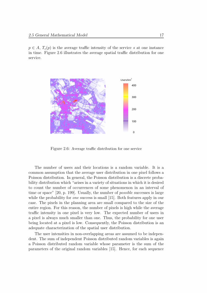
The mobile users M are given by a traffic snapshot. This is a staticrealization of the average user demand obtained on basis of spatial averagetraffic load distributions. A traffic snapshot gives detailed information onthe position, mobility, and service of each user. The average spatial trafficdistribution of a service s ∈ S is denoted by Ts : A → R+. For a position
2.5 General Mathematical Model 17
p ∈ A, Ts(p) is the average traffic intensity of the service s at one instancein time. Figure 2.6 illustrates the average spatial traffic distribution for oneservice.
Figure 2.6: Average traffic distribution for one service
The number of users and their locations is a random variable. It is acommon assumption that the average user distribution in one pixel follows aPoisson distribution. In general, the Poisson distribution is a discrete proba-bility distribution which “arises in a variety of situations in which it is desiredto count the number of occurrences of some phenomenon in an interval oftime or space” [20, p. 199]. Usually, the number of possible successes is largewhile the probability for one success is small [15]. Both features apply in ourcase. The pixels in the planning area are small compared to the size of theentire region. For this reason, the number of pixels is high while the averagetraffic intensity in one pixel is very low. The expected number of users ina pixel is always much smaller than one. Thus, the probability for one userbeing located at a pixel is low. Consequently, the Poisson distribution is anadequate characterization of the spatial user distribution.
The user intensities in non-overlapping areas are assumed to be indepen-dent. The sum of independent Poisson distributed random variables is againa Poisson distributed random variable whose parameter is the sum of theparameters of the original random variables [15]. Hence, for each sequence
18 2 Preliminaries
(An)n∈N, An ⊂ A, of pairwise disjoint sets following equation applies:
Ts
(
⋃
n
An
)
=∑
n
Ts(An). (2.2)
Furthermore, Ts(∅) = 0 holds. These properties show that Ts is a measure onA [9]. Actually, it is a counting measure which maps to a region the expectednumber of users in it. This measure is finite, that is, Ts(A) < ∞ since weonly consider situations in which the traffic intensity in the entire planningarea is finite.
We assume that the number of users for each service s ∈ S in a certainregion A ⊆ A is proportional to the size of the region λd(A). The measure λd
is the d-dimensional Lebesgue-Measure. We assume that there exists a userdensity fs : A → R+ for each service s ∈ S. The expected number of usersof service s in area A is thus expressed by
Ts(A) =
∫
p∈A
fs(p) dp. (2.3)
2.5.3 CIR Constraints and Blocking
At first, we derive the complete CIR constraints for the uplink and downlinkdirection. The average CIR targets for a mobile station m ∈ M are denotedby µ↑
m for uplink and µ↓m for downlink. Furthermore, there are transmit ac-
tivity factors α↑m and α↓
m for every mobile indicating the average ratio of timeit is transmitting data on the radio channel. In speech conversations, for ex-ample, every user speaks on average 50% of the time. The CIR inequalityhas to be satisfied in active periods only. At other instances in time, thereis no data transmission. For this reason, we assign a transmit activity factorof one to the desired mobile. We do not know if the signals of other usersare currently in an active period or not. Therefore, we apply the transmitactivity factors to the other signals in (2.1) in order to consider the averageinterference power. Finally, γ↑
mi in uplink and γ↓im in downlink are the atten-
uation factors for mobile station m ∈ M and base station antenna i ∈ N .Apart from the path loss between the mobile and the antenna, additionallosses and gains are included dependent on the cabling, hardware, and userequipment.
In the uplink direction, the transmission power of a mobile m ∈ Mis denoted by p↑m. Then the strength of the desired signal at base stationantenna i ∈ N is γ↑
mi p↑m. The received background noise at antenna i is
marked by ηi. With these conventions, the basic CIR target inequality (2.1)

2.5 General Mathematical Model 19
for the uplink transmission from mobile m to antenna i reads as:
γ↑mi p
↑m
∑
n 6=m γ↑ni α
↑n p↑n + ηi
≥ µ↑m. (2.4)
Several base stations use the same frequency band (cf. Section 2.4.1). In thismodel, we assume that all base stations use the same frequency spectrum.Hence, all users in the area convey information in the same frequency bandat the same time. All these transmissions are received with varying strengthby each base station antenna. For mobile stations using another frequencyband in reality, the attenuation factor is appropriately low. The average totalreception power at antenna i ∈ N is thus given by
p↑i :=∑
m∈M
γ↑mi α
↑m p↑m + ηi. (2.5)
As mentioned previously, it is not known for a link whether it is active ornot. For this reason, we take the transmit activity factors of the mobilesinto account and obtain the average power. Using the last equation, (2.4)simplifies to
γ↑mi p
↑m
p↑i − γ↑mi α
↑m p↑m
≥ µ↑m. (2.6)
In the downlink direction, the pilot and common channels are included,whose power we denote by p
(c)i at base station antenna i ∈ N . This value
is assumed to be constant. Furthermore, p↓im is the strength of the signalfrom antenna i to mobile m and ωm ∈ [0, 1] is an environment dependentorthogonality factor. The signals an antenna transmits to its associated mo-biles partly lose their orthogonality due to multipath propagation (cf. Sec-tion 2.4.1). If ωm = 0 holds, the signals are perfectly orthogonal and ωm = 1means no orthogonality. The average total transmission power of antenna iis defined by
p↓i :=∑
m∈Mi
α↓m p↓im + p
(c)i . (2.7)
We denote by ηm the noise at mobile m. Then the CIR constraint in downlinksatisfies following inequality:
γ↓im p↓im
γ↓im ωm
(
p↓i − α↓m p↓im
)
+∑
j 6=i γ↓jm p↓j + ηm
≥ µ↓m. (2.8)
The transmission power of a base station antenna is restricted. Typically,a UMTS antenna cannot emit more than 20W. In addition, there are limits
20 2 Preliminaries
on the average load of a cell. These load limits lie significantly below 100%since it is important to have a buffer to compensate for dynamic effects. Thedownlink load is defined as the ratio of the current transmission power to themaximum possible output power. Usually, the limit of the downlink load liesat 70%. The uplink load is given by 1 − 1
noise rise. The noise rise is the ratio
of the total received power at a base station antenna to the noise power. Theuplink load should not rise above 50%. We denote by Πmax↓
i the maximumpossible transmission power and by pmax↑
i and pmax↓i the maximum allowed
reception and transmission power of a base station antenna i ∈ N . Thelatter can be derived by resolving
1 −ηi
pmax↑i
= load limit↑ andpmax↓
i
Πmax↓i
= load limit↓.
Throughout this thesis, we mean with “maximum total power” the maximumallowed total power pmax↑
i and pmax↓i , respectively.
The following inequalities express that on average all users in cell i areserved and thus no blocking occurs:
p↑i ≤ pmax↑i and p↓i ≤ pmax↓
i . (2.9)
Using equations (2.5) and (2.7), this can be transformed into
∑
m∈M
γ↑mi α
↑m p↑m ≤ pmax↑
i − ηi and∑
m∈Mi
α↓m p↓im ≤ pmax↓
i − p(c)i . (2.10)

3 Existing Methods
In this chapter, we discuss established methods to assess the average blockingrate of a base station antenna in a UMTS radio network. First, we introducean approach to approximate the blocking rate based on a system of equations.This system can be set up for one traffic snapshot as described in the first partof the following section. In order to obtain statistically reliable results, suchequation systems have to be solved for a large number of snapshots. Sincethe computational complexity of this procedure is too high to be applicablein some situations, the basic idea of this approach is generalized on the basisof average traffic load distributions. This idea is explained afterwards. Thismethod speeds up calculation radically. In exchange, it causes a significantunderestimation of the blocking rate of a cell in a region under around 5%. Inthe next section, the so-called Monte Carlo simulation on traffic snapshotsis described briefly. This is a popular method but this approach is veryextensive and time consuming. The snapshot based system of equations isalso a Monte Carlo simulation. The last section summarizes the shortcomingsof the formerly presented methods.
The notation can be found in Appendix A. Throughout this thesis, weassume perfect power control on dedicated channels. That is, the CIR tar-gets are met at equality. Moreover, no user is in soft handover, and effects ofshadow fading are neglected. Uplink and downlink are considered indepen-dently.
3.1 System of Equations
In this section, the ideas from [6] are introduced briefly. A system of equa-tions is set up for uplink and downlink respectively describing the averagetransmission and reception powers of the antennas in the radio network.These results are then used to assess the blocking rate of each cell.
First, the equations are derived based on a traffic snapshot and thengeneralized on the basis of stochastical average load. Afterwards, we point
21

22 3 Existing Methods
out how the blocking rate is calculated in both cases. This model is thebasic principle of the method we develop in the next chapters. Throughoutthis thesis, the indices i and j will be used for base station antennas. Thesubscript i denotes the cell whose blocking rate we wish to determine. Avector with elements vj is denoted in bold font v. Moreover, diag (v) marksa diagonal matrix having the same dimension as v and the components of v
on the main diagonal.
3.1.1 Snapshot Based Derivation
We consider a set M of mobile stations given by a traffic snapshot. Followingassumptions are made in this model for the time being:
(i) limitations of transmission powers and noise rise are neglected and
(ii) all users are served.
These restrictions are important for the derivation of the equations. Later,they will be abolished when blocking is modeled.
Uplink
In the uplink direction, we start from equation (2.5), which describes theaverage reception power of antenna i, written as
p↑i =∑
m∈Mi
γ↑mi α
↑m p↑m +
∑
j 6=i
∑
m∈Mj
γ↑mi α
↑m p↑m + ηi. (3.1)
In this way, it can be recognized that the total reception power at an antennaconsists of three parts: one portion for the interference from the own andfrom the other cells respectively and the noise exterior to the system. Forthe uplink CIR target to be maintained by transmission from mobile stationm ∈ M to antenna i ∈ N , inequality (2.6) must hold. As stated in thebeginning, we assume that equality applies. When converting this equationproperly and defining the uplink user load of a mobile m as
l↑m :=α↑
m µ↑m
1 + α↑m µ↑
m
, (3.2)
the uplink coupling factors result in
C↑ij :=
∑
m∈Mj
γ↑mi
γ↑mj
l↑m. (3.3)

3.1 System of Equations 23
Consequently, with (3.1) and (3.3), the uplink transmission power of basestation antenna i reads as
p↑i = C↑ii p
↑i +
∑
j 6=i
C↑ij p↑j + ηi. (3.4)
We call the matrixC↑ :=
(
C↑ij
)
1≤i,j≤|N |
the uplink cell load coupling matrix (uplink coupling matrix). The compo-nents of C↑ can be interpreted in following way. The diagonal entry C↑
ii
measures the contribution from the intra-cell interference to the total re-ceived power. The value C↑
ij scales the inter-cell interference contributionfrom antenna j 6= i. The desired system of equations arises from (3.4):
p↑ = C↑ p↑ + η↑. (3.5)
The solution of this system is the vector with the uplink reception powers ateach base station antenna.
Downlink
The same approach is applied in the downlink case. The total average outputpower of base station antenna i ∈ N is defined by (2.7). The CIR constraintis given by (2.8). Again, the assumption of perfect power control holds andthe constraint is an equation. The downlink user load reads as
l↓m :=α↓
m µ↓m
1 + ωm α↓m µ↓
m
. (3.6)
We use it to introduce the downlink coupling factors
C↓ii :=
∑
m∈Mi
ωm l↓m and C↓ij :=
∑
m∈Mi
γ↓jm
γ↓im
l↓m (j 6= i) (3.7)
for antennas i and j, as well as the traffic noise power of sector i
p(η)i :=
∑
m∈Mi
ηm
γ↓im
l↓m. (3.8)
The meaning of the coupling factors C↓ij is the following. The diagonal entry
C↓ii represents the contribution from the intra-cell interference to the total
transmission power. The value C↓ij specifies the portion of transmission power

24 3 Existing Methods
allocated on overcoming the inter-cell interference from antenna j 6= i. Theitem p
(η)i expresses the fraction of transmission power spent on overcoming
the noise at the mobiles if there was no intra-system interference. For thetransmission power at antenna i we obtain
p↓i = C↓ii p
↓i +
∑
j 6=i
C↓ij p↓j + p
(η)i + p
(c)i . (3.9)
The matrix
C↓ :=(
C↓ij
)
1≤i,j≤|N |
is called the downlink cell load coupling matrix (downlink coupling matrix).Equation (3.9) for each base station antenna yields the following system ofequations
p↓ = C↓p↓ + p(η) + p(c). (3.10)
The solution of this system is the downlink transmission power for every cell.
3.1.2 Expected Coupling
The coupling matrices C↑ and C↓ are stochastical. They depend on the posi-tions and services of the active mobiles. We assume the user distribution inthe planning area to be known (cf. Section 2.5.2). The matrix entries definedin (3.3) and (3.7) are linear compositions. For this reasons, it is possible todetermine the expected values of the load coupling matrices, denoted by C↑
and C↓. Then, the equation systems (3.5) and (3.10) can be set up withthese expected values.
For a clearer presentation, it is implied, that we have representative CIRtargets µ↑
s, µ↓s and transmit activity factors α↑
s, α↓s in both directions for each
service s ∈ S. Furthermore, ηp is the noise and ωp the orthogonality factorat a mobile in position p. The attenuation factors between a base stationantenna i and a user located in p are denoted by γ↑
pi in uplink and γ↓ip in
downlink.
The definitions of the user load (3.2) and (3.6) are substituted by
l↑p :=∑
s∈S
α↑s µ↑
s
1 + α↑s µ↑
s
Ts(p) and l↓p :=∑
s∈S
α↓s µ↓
s
1 + ωp α↓s µ↓
s
Ts(p). (3.11)
Remember, that Ts(p) is the expected value of the traffic intensity for service sat location p. The other factors in the above definitions are constants. Thus,l↑p and l↓p are the expected values of l↑m and l↓m at location p. We derive the

3.1 System of Equations 25
entries of the expected uplink coupling matrix by
C↑ii :=
∫
p∈Ai
l↑p dp , C↑ij :=
∫
p∈Aj
γ↑ip
γ↑jp
l↑p dp. (3.12)
The components of the expected downlink coupling matrix and traffic noisepower read as
C↓ii :=
∫
p∈Ai
ωp l↓p dp , C↓ij :=
∫
p∈Ai
γ↓jp
γ↓ip
l↓p dp , p(η)i :=
∫
p∈Ai
ηp
γ↓ip
l↓p dp. (3.13)
3.1.3 Approximating Blocking
Until now, the system of linear equations introduced in the former sectionsignores the effects due to load control which is triggered if the power of acell would excess its limit (cf. Section 2.4.3). To mimic load control, theapproach from [7] is adopted to reduce the load in saturated cells. In thisproposed model, it is not necessary to distinguish whether a user is rejectedor whether the service quality of other users is downgraded. Following twoproperties characterize a proper load control:
(i) Admissibility : After load control has been applied, all antenna powervalues are feasible, that is, (2.10) holds.
(ii) Greediness: Users are only rejected by a cell if it cannot serve themwithout rising above its own capacity. That is, an antenna does notreject users to ease the situation of its neighboring cell.
Furthermore, we assume that a base station antenna is able to serve all itsusers up to a certain fraction of their resource demands. This is realized byscaling the relative user load ( (3.2) and (3.6) or (3.11) ) in the according cellby a value λ between 0 and 1. In doing so, only as little load as necessary iswithdrawn. The blocking rate is then 1−λ. However, in realistic settings, theassumption of compressible user demand is not valid. The obtained scalingvectors can be used as a guideline for determining how many mobiles needto be refused.
A complementarity condition has to hold for the resulting power andscaling vectors in order to achieve the above two properties. In general,in a complementarity condition one or several subgroups of inequalities arecomprised. In each group at least one of these inequalities should be met atequality [4]. In our case, it claims that if user demand in a cell is reduced,then the cell power is equal to its maximum allowed value.

26 3 Existing Methods
The in the following described procedure can be applied to both kinds ofequation system: the one derived by snapshot analysis and the one obtainedon the basis of stochastical average load. For this reason, we simply use thenotation we introduced in Section 3.1.1 for the traffic noise power vector aswell as for the coupling matrices. The power vector obtained by this scalingprocedure is denoted by p↑ and p↓, respectively. The approach using theexpected coupling matrices yields an approximation of the expected blockingrate. We explain the method for the downlink direction first since this is theeasier one. The approach in uplink is more complex because scaling is appliedto columns instead of rows.
Downlink
In the downlink direction, the rows of the load coupling matrix have to bescaled, that is,
p↓ = diag(
λ↓)
· C↓ · p↓ + diag(
λ↓)
· p(η) + p(c). (3.14a)
Due to the linear definitions of the matrix entries and the entries of thetraffic noise power vector, scaling the user load is equal to scaling the loadcoupling matrix and the traffic noise power. The complementarity conditionis expressed by
λ↓i < 1 =⇒ p↓i = pmax↓
i . (3.14b)
The scaling vector λ and the corresponding transmit power estimates areobtained by following recursion formula provided that 0 < p
(c)i ≤ pmax↓
i and∑
j C↓ij > 0 for all i:
With the initial settingsλ0
i = 1
p0i = p
(c)i ,
the update step is given by
λt+1i = min
{
λti,
pmax↓i − p
(c)i
C↓ii p
max↓i +
∑
j 6=i C↓ij pt
j + p(η)i
}
pt+1i =
1
1 − λt+1i C↓
ii
[
p(c)i + λt+1
i
(
∑
j 6=i
C↓ij p
tj + p
(η)i
)]
.
(3.15)
The resulting sequences have the properties
1 = λ0i ≥ λ1
i ≥ λ2i ≥ . . . ≥ 0,
p(c)i = p0
i ≤ p1i ≤ p2
i ≤ . . . ≤ pmax↓i ,
3.2 Monte Carlo Simulation 27
andλt
i < 1 =⇒ pti = pmax↓
i .
The sequences (λsi )s≥0 and (ps
i )s≥0 converge since they are component-wisemonotonous and bounded. Their limiting values represent a complemen-tary solution to (3.14), that is, a feasible solution to (3.14a) that fulfills thecomplementarity condition (3.14b). This solution is unique.
Uplink
In the uplink case, the columns of the load coupling matrix are scaled:
p↑ = C↑ · diag(
λ↑)
· p↑ + η↑. (3.16a)
The complementarity condition looks as follows
0 < λ↑i < 1 =⇒ p↑i = pmax↑
i
p↑i > pmax↑i =⇒ λ↑
i = 0.(3.16b)
One method to determine a complementary solution to (3.16) is to ex-press the problem as a so-called extended linear complementarity problem.Essentially, this is a linear feasibility problem where in addition at least onecomplementarity condition is given [4]. The purpose of this thesis is not todescribe the technique to solve this problem. Therefore, the interested readeris referred to [7]. The important point is that the problem is solvable. Incontrast to the downlink direction, the solutions to (3.16) are not unique.
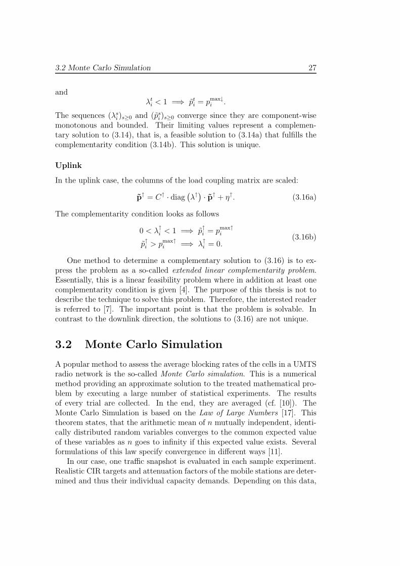
3.2 Monte Carlo Simulation
A popular method to assess the average blocking rates of the cells in a UMTSradio network is the so-called Monte Carlo simulation. This is a numericalmethod providing an approximate solution to the treated mathematical pro-blem by executing a large number of statistical experiments. The resultsof every trial are collected. In the end, they are averaged (cf. [10]). TheMonte Carlo Simulation is based on the Law of Large Numbers [17]. Thistheorem states, that the arithmetic mean of n mutually independent, identi-cally distributed random variables converges to the common expected valueof these variables as n goes to infinity if this expected value exists. Severalformulations of this law specify convergence in different ways [11].
In our case, one traffic snapshot is evaluated in each sample experiment.Realistic CIR targets and attenuation factors of the mobile stations are deter-mined and thus their individual capacity demands. Depending on this data,
28 3 Existing Methods
the power levels of all active connections in the system are calculated. Theinput and output powers are assigned to every antenna in the radio networkaccording to (2.5) and (2.7). If these powers exceed the maximum valuesone or more connections are dropped until the capacity constraints (2.10)are fulfilled. In this way, the blocking rate of every cell can be assessed.There are various methods to evaluate the radio network performance basedon one traffic snapshot. Besides static or dynamic simulations of the system(cf. [21]) a snapshot based set of equations can be solved as described in theSections 3.1.1 and 3.1.3.
The results of several independent snapshot analysises are combined toobtain statistically significant results. In this connection, we want to knowhow precise the estimated solution is for a certain number of trials, calledthe sample size. For this reason, the confidence interval is determined. Thisis a numerical interval covering the true value of the wanted unknown witha specified probability. That is, we find a value δ > 0 such that
P(x ∈ [x − δ, x + δ]) = 1 − α (3.17)
for a given confidence level 1− α. The value x denotes the true value of theblocking rate and x is the solution obtained by the Monte Carlo simulation.For techniques to assess the interval [x − δ, x + δ] refer to [17, 10].
Usually, the sample size is very large if one wants to ensure statisticalaccuracy. Hundreds or even thousands of snapshots have to be analyzed toachieve statistically significant results [6]. For this reason, this method is verytime-consuming and extensive. This procedural problem gets even worse if anevaluation of the network load shall be used within a local search procedurewhere it has to be executed several times. Consequently, the Monte Carlosimulation achieves accurate results at the expense of a high complexity thatlimits the applicability of this method.
3.3 Shortcomings
The problem of the snapshot based model was already highlighted in Sec-tion 3.2. The computational effort of this method is just too high for somepurposes. In order to reduce this complexity, the approach using the expectedcell load coupling matrix is applied. This is much less time consuming. How-ever, this method produces estimation errors in the power values and theblocking rate. These errors are particularly significant for the blocking ratesince the tolerable values are very small. We aim at designing radio networkswith blocking rates lower than 2%. Due to this low limit of tolerance, theexpected coupling approach should be improved for our purpose.

3.3 Shortcomings 29
Figure 3.1 illustrates this effect schematically in case of a network with asingle base station antenna for the downlink direction. Figure 3.1(a) showsthe blocking rate of the cell and Figure 3.1(b) the power of the antennadepending on the average number of users in the cell. The green curve ineach picture represents the results of the expected coupling approach fromSection 3.1.2. The red one shows the exact values which can be describedanalytically for this simple case. The exact values can be understood as theexpected values of the power and the blocking rate, respectively. That is,the power or blocking rate of all possible snapshot situations is weighted bythe probability for the according traffic snapshot to occur and summed up.
0,05
0,25
0,2
0,0
75
Blo
ckin
g R
ate
0,3
0,15
0,1
Average Number of Users
25 10050
Expected Coupling
Exact
(a) Blocking rate
Pow
er [W
]
Average Number of Users
75
10,0
25 50
5,0
100
7,5
2,5
Expected Coupling
Exact
(b) Power
Figure 3.1: Power and blocking rate in downlink for an isolated cell
In Figure 3.1(a), it is remarkable that the blocking rate obtained by theexpected coupling approach is zero upto a certain point. Then the curve hasan abrupt, steep rise. At this inflection point, the scaling factor computedaccording to (3.15) is smaller than one for the first time. By contrast, theexact blocking rate rises much earlier. This value is already greater than zeroif in one traffic snapshot situation blocking occurs in the cell. Such effectsof randomness are ignored by using average traffic load distributions. Thisstatistical data specifies the expected amount of traffic in the radio network.Possible variations from this expected value are not taken into account.
Figure 3.1(b) depicts that the expected coupling method tends to under-estimate the power in the low region under around 9W. The reason is thatthe power is a convex, monotonically increasing function of the average userintensity. Snapshot situations with more users than expected increase the
30 3 Existing Methods
power of a base station antenna above average. In the concerned region ofaverage user density, the number of users is distributed almost symmetricallyaround its expected value. That is, traffic situations with more users than ex-pected are as possible as those with less users than expected. Therefore, theexpected power value of all possible traffic snapshots is higher than that ob-tained by the expected coupling method. In the higher region from shortlybelow the maximum power, the expected coupling approach overestimatesthe power. This is due to the fact that the maximum power is not exactlymet in reality. If there is more than one antenna in the radio network thisoverestimation of the other antennas’ powers leads to an overestimation ofthe blocking rate in the considered cell in this high region.
In conclusion, there are methods to determine the average blocking ratealmost exactly with high computational effort on the one hand. On the otherhand, we have a model that has an acceptable complexity but whose resultsneed to be improved for our purpose. Such improvements are developed andanalyzed in the rest of this thesis.

4 The Blocking Rate
as Expected Value
The goal of this diploma thesis is to develop a mathematical model to effi-ciently approximate the blocking rates of the cells in a UMTS radio network.Efficiently in this case means that the new method shall have about the speedof the expected coupling approach of the former chapter and about the ac-curacy of Monte Carlo simulation. In this chapter, we propose a new modelto solve this task.
The basis for the following considerations is the expected coupling ap-proach introduced in Section 3.1.2 and the computation of the blocking rategiven in Section 3.1.3. We aim at reducing the inaccuracies of this methodwith regard to the blocking rate (cf. Section 3.3). These inaccuracies are dueto the fact that the expected coupling approach neglects effects of random-ness. These effects can be taken into account by approximating the blockingrate of a cell by its expected value. This is the idea of the model presentedin this chapter. We determine the expected value of the average blockingrate depending on the intra-cell interference. In this model, we make twoessential simplifications:
(1) The mobile stations in the own cell are modeled independently of theirlocations, that is, we consider average users within the own sector.
(2) We use constant estimates for the inter-cell interference.
For didactical reasons, we first address the case that all users in a sectorhave constant load l↑m and l↓m, respectively. In this case, the average blockingrate of an antenna can be expressed depending on the number of users inthe cell. In the next step, we examine the situation in which the user loadwithin the sector varies. In this case, the discrete approach is not suitable.Instead, we compute the expected value of the blocking rate depending onthe main-diagonal entry of the load coupling matrix. We assume that thisrandom variable follows a normal distribution. Afterwards, an enhancement
31

32 4 The Blocking Rate as Expected Value
of the model is proposed, which possibly improves the estimates of the inter-cell interference. Finally, we discuss the assumption that the main-diagonalmatrix entry is normally distributed.
4.1 Constant User Load
The sketch of modeling the intra-cell interference stochastically is descriptivein the case that all users in the cell have equal load l↑m, l↓m. We are able tomodel the intra-cell interference depending on the number of users in thesector. Thus, it is possible to specify the capacity of a cell explicitly and tocompute the expected value of the average blocking rate depending on thiscapacity. In reality, the case of constant user load could be achieved if allmobile stations in the cell request the same service, have the same velocity,user equipment, and orthogonality factor. Of course, such a setting is notrealistic. However, it serves to introduce the model in an easy way.
This section is organized as follows. First, we give the basic formula of theexpected value of the average blocking rate. Moreover, we define the basicvariables capacity and average blocking rate of a sector. Then, the capacityof a cell is computed in uplink and downlink. In the downlink direction, arefinement is shown since the inter-cell interference power also depends onthe number of users in the own sector. Afterwards, we extend the model tothe case that the user load within a cell is not constant but its variation issmall. In the following, we denote the constant user load in cell i by l↑i andl↓i , respectively. The number of users in sector i is expressed by n ∈ N.
4.1.1 Preliminaries
The average blocking rate at base station antenna i is denoted by b↑i in uplinkand b↓i in the downlink direction. The common formulas for the expectedvalue of the average blocking rate of the sector depending on the user numbern are given by
E[b↑i ] =∞
∑
n=0
b↑i (n) P(n) and E[b↓i ] =∞
∑
n=0
b↓i (n) P(n). (4.1)
Here, P(n) denotes the probability of exactly n mobiles being located in cell i.We assume that the traffic intensity for one service in a cell is a random vari-able that follows a Poisson distribution with parameter Ti (cf. Section 2.5.2).Knowing the average traffic intensity Tp of the available service in location p
4.1 Constant User Load 33
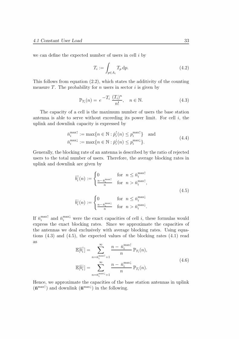
we can define the expected number of users in cell i by
Ti :=
∫
p∈Ai
Tp dp. (4.2)
This follows from equation (2.2), which states the additivity of the countingmeasure T . The probability for n users in sector i is given by
PTi(n) = e
−Ti (Ti)n
n!, n ∈ N. (4.3)
The capacity of a cell is the maximum number of users the base stationantenna is able to serve without exceeding its power limit. For cell i, theuplink and downlink capacity is expressed by
nmax↑i := max{n ∈ N : p↑i (n) ≤ pmax↑
i } and
nmax↓i := max{n ∈ N : p↓i (n) ≤ pmax↓
i }.(4.4)
Generally, the blocking rate of an antenna is described by the ratio of rejectedusers to the total number of users. Therefore, the average blocking rates inuplink and downlink are given by
b↑i (n) :=
{
0 for n ≤ nmax↑i
n− nmax↑i
nfor n > nmax↑
i ,
b↓i (n) :=
{
0 for n ≤ nmax↓i
n− nmax↓i
nfor n > nmax↓
i .
(4.5)
If nmax↑i and nmax↓
i were the exact capacities of cell i, these formulas wouldexpress the exact blocking rates. Since we approximate the capacities ofthe antennas we deal exclusively with average blocking rates. Using equa-tions (4.3) and (4.5), the expected values of the blocking rates (4.1) readas
E[b↑i ] =
∞∑
n=nmax↑i
+1
n − nmax↑i
nPTi
(n),
E[b↓i ] =
∞∑
n=nmax↓i +1
n − nmax↓i
nPTi
(n).
(4.6)
Hence, we approximate the capacities of the base station antennas in uplink(nmax↑) and downlink (nmax↓) in the following.

34 4 The Blocking Rate as Expected Value
4.1.2 Uplink
Due to assumption (1), the main diagonal entry of the load coupling matrixdepends merely on the number of users in the sector. That is,
C↑ii(n) = n l↑i . (4.7)
Because the number of users in the cell is Poisson distributed, C↑ii follows a
scaled Poisson distribution with scaling factor l↑i . Since C↑ii depends on the
user intensity n, the power p↑i depends on n, too. Substituting C↑ii according
to (4.7), the equation for the reception power at base station antenna i readsas
p↑i (n) = n l↑i p↑i (n) +∑
j 6=i
C↑ij p↑j + ηi. (4.8)
The power values C↑ij for j 6= i are defined by
C↑ij := C↑
ij λ↑j .
The values p↑j are the solutions of the equation system (3.16) using the ex-pected coupling matrix. According to assumption (2), we estimate the inter-cell interference by average values. In doing so, we use C↑
ij instead of C↑ij in
order to express the realistic behavior of antenna j. Cell j only serves thefraction of users that does not exceed its available radio resources. The otherportion is blocked. We assume that
∑
j 6=i
C↑ij p↑j + ηi > 0.
For this reason, with (4.8) it holds that
p↑i (n) > n l↑i p↑i (n).
This is equivalent to1 − n l↑i > 0. (4.9)
In cell i, blocking happens if more than nmax↑i active users are in the
sector. Then, the surplus will not be served. In this case, the total receivedpower of the antenna is p↑i (n
max↑i ) ≤ pmax↑
i . Transforming (4.8), the averageuplink power for n mobile stations in the cell satisfies the expression
p↑i (n) =
P
j 6=i C↑ij p
↑j+ηi
1 − n l↑i
for n ≤ nmax↑i
p↑i (nmax↑i ) for n > nmax↑
i .(4.10)

4.1 Constant User Load 35
Due to (4.9), this formula is well defined. In order to assess the capacity ofthe cell we use the above equation in definition (4.4) of nmax↑
i . This resultsin
nmax↑i = max
{
n ∈ N :
∑
j 6=i C↑ij p↑j + ηi
1 − n l↑i≤ pmax↑
i
}
.
From the above equation, nmax↑i can be derived as
nmax↑i =
⌊
pmax↑i −
∑
j 6=i C↑ij p↑j − ηi
pmax↑i l↑i
⌋
. (4.11)
We round down the received value since the number of users in a cell isintegral.
4.1.3 Downlink
Now, we follow the same considerations in downlink. In contrast to the uplinkdirection, the traffic noise power p
(η)i has to be taken into account, but this
issue is ignored for the time being. In addition to the constant user load l↓i ,we also assume a constant orthogonality factor in the whole cell area. Wedenote this unique orthogonality factor by ωi. The main diagonal entry ofthe downlink coupling matrix in case of n users in sector i is given by
C↓ii(n) = n ωi l
↓i . (4.12)
Therefore, the average transmission power of antenna i depending on theuser intensity n in the cell reads as
p↓i (n) = n ωi l↓i p↓i (n) +
∑
j 6=j
C↓ij p↓j + p
(c)i . (4.13)
The scaled off-diagonal entries of the coupling matrix are defined as
C↓ij := λ↑
i C↓ij.
The value p↓j is the solution of the scaled, expected value based equation
system (3.14). The values C↓ij estimate the fraction of the average total
power at antenna i that is necessary to overcome the received power of otherantennas at the mobiles in sector i. If some of them are blocked, theseestimates are lower. We involve the scaling in order to take the blockingbehavior of our own cell into account. Following expression is satisfied dueto p
(c)i > 0:
∑
j 6=i
C↓ij p↓j + p
(c)i > 0.

36 4 The Blocking Rate as Expected Value
Therefore, it holds that
p↓i (n) > n ωi l↓i p↓i (n).
This can be transformed into
1 − n ωi l↓i > 0. (4.14)
If there are more users in the cell than nmax↓i , blocking happens such
that the total transmission power does not exceed its limit. For this reason,equation (4.13) can be written as
p↓i (n) =
P
j 6=i C↓ij p
↓j +p
(c)i
1 − n ωi l↓i
for n ≤ nmax↓i
p↓i (nmax↓i ) for n > nmax↓
i .
Because of (4.14), this expression is well defined. Using the above formulationin the definition (4.4) of nmax↓
i , we obtain
nmax↓i = max
{
n ∈ N :
∑
j 6=i C↓ij p↓j + p
(c)i
1 − n ωi l↑i
≤ pmax↑i
}
.
This can be transformed into
nmax↓i =
⌊
pmax↓i −
∑
j 6=i C↓ij p↓j − p
(c)i
pmax↓i ωi l
↓i
⌋
.
With this closed-form expression, we are able to calculate the quantity nmax↓i
as well as the desired expected value of the average blocking rate accordingto (4.6).
Refined Downlink
In the above approach, the contributions of other antennas to the interferencein the own cell are not modeled stochastically. We use constant expectedvalues. However, in downlink, it is possible to additionally vary the off-diagonal entries of the load coupling matrix C↓ in order to obtain moreprecise results.
The coupling factors C↓ij describe the fraction of total transmission power
of antenna i spent on overcoming the interference originating in sector j.Each new request in cell i causes the transmission power of the antenna toits associated mobiles to increase. At the same time, this new user is affectedby interference from other base station antennas. That is, the interference

4.1 Constant User Load 37
power in sector i increases and the antenna has to raise the power to overcomethis interference. Actually, the strength of the interference power dependson the location of the affected mobile. Users at the cell border are muchmore exposed to inter-cell interference than mobiles in the center of thesector. We do not consider the positions of the mobile stations in our owncell (condition (1)). Instead, we assume average users in the sector. Sincethe off-diagonal entries C↓
ij depend on the number of users in cell i we assume
a proportional correlation between C↓ij and the average number of users in
sector i. In uplink, a similar approach is not possible because the inter-cellinterference depends on the number of mobiles in the other cells, which wedo not model stochastically.
Instead of (4.13), the total transmission power of antenna i is calculatedas
p↓i (n) = n ωi l↓i p↓i (ni) + n∑
j 6=i
C↓ij
Ti
p↓j + p(c)i
with Ti as defined in (4.2). The value C↓ij is an entry of the expected load
coupling matrix. We assume the inter-cell interference to be uniformly dis-tributed to all mobiles in sector i. Therefore, in place of being scaled, theoff-diagonal entries of C↓are normalized by the average user intensity in cell i.As in (4.13), p↓j is the total transmission power of antenna j received by sol-ving the equation system with the scaled, expected coupling matrix. Theapproximated transmission power of base station antenna i is thus:
p↓i (n) =
n 1Ti
P
j 6=i C↓ij p
↓j + p
(c)i
1 − n ωi l↓i
for n ≤ nmax↓i
p↓i (nmax↓i ) for n > nmax↓
i .
Then the approximated capacity of cell i is determined according to
nmax↓i =
⌊
pmax↓i − p
(c)i
pmax↓i ωi l↓i + 1
Ti
∑
j 6=i C↓ij p↓j
⌋
.
The Traffic Noise Power
The traffic noise power in downlink in cell i is modeled in analogy to theexpected coupling approach. We estimate it by the expected value
p(η)i :=
∫
p∈Ai
ηp
γ↓ip
l↓p dp.
The traffic noise power of an antenna depends on the number of mobiles inits best server area. The reason is the same as for the dependence of the

38 4 The Blocking Rate as Expected Value
off-diagonal coupling matrix entries on the number of mobiles. The moreusers an antenna serves, the more power it has to spent on overcoming thenoise at these mobiles. Therefore, we normalize the average noise power bythe average user intensity in the cell and multiply this value with the usernumber n. Finally, the approximated total transmission power of antenna ifor n mobiles in the cell results in
p↓i (n) = n ωi l↓i p↓i (n) + ni
1
Ti
(
∑
j 6=i
C↓ij p↓j + p
(η)i
)
+ p(c)i .
This can be transformed into
p↓i (n) =
n 1Ti
(
P
j 6=i C↓ij p
↓j +p
(η)i
)
+ p(c)i
1 − n ωi l↓i
for n ≤ nmax↓i
p↓i (nmax↓i ) for n > nmax↓
i .(4.15)
In analogy to the previous sections, the capacity of cell i is derived as
nmax↓i =
⌊
pmax↓i − p
(c)i
pmax↓i ωi l
↓i + 1
Ti
(∑
j 6=i C↓ij p↓j + p
(η)i
)
⌋
. (4.16)
4.1.4 Extension
The proposed discrete approach is valid in cases in which the variation of theuser load l↑m and l↓m, respectively, within the sector is small such that it canbe represented by its average value without being too unprecise. In reality,this situation could occur if all mobile stations in the cell request the sameservice but have each a different velocity, user equipment or orthogonalityfactor. We determine the average user load over all positions in the sectorand assume it to be constant for every mobile station. That is, we transformthis situation into the case with constant user load.
In mathematical models, it is common to classify the user mobility coarselyinstead of considering speed as a continuous variable. One possible classifica-tion is to group the different mobility types according to the average velocity.E.g. the mobility type pedestrian has the speed 1 m/s. In the following, Mdenotes the set of mobility types.
Uplink
For every position p ∈ Ai, we compute the expected value of the user load.This yields
l↑p =∑
m∈M
l↑m Tp Pp(m).

4.1 Constant User Load 39
In this formula, Tp is the average traffic intensity in point p. The value Pp(m)is the probability for the presence of a user having mobility type m at thislocation and l↑m is the uplink user load for mobility type m. This user loadis given by
l↑m =α↑
m µ↑m
1 + α↑m µ↑
m
,
which is the same definition as (3.2) for the user load of a mobile station.The average uplink user load for a mobile in cell i reads as
l↑i :=1
Ti
∫
p∈Ai
l↑p dp. (4.17)
In fact, this is the main-diagonal entry of the expected cell load couplingmatrix C↑ normalized by the average number of users in the according sector.The constant user load l↑i is used in the equations (4.10) and (4.11) in orderto derive a formula for the uplink capacity of cell i.
Downlink
In analogy to the uplink, the expected value of the downlink user load inposition p ∈ Ai is given by
l↓p =∑
m∈M
l↓m(p) Tp Pp(m)
with Tp and Pp(m) as explained before. The downlink user load for a userwith mobility type m at location p reads as
l↓m(p) =α↓
m µ↓m
1 + ωp α↓m µ↓
m
.
Besides the mobility type m, the user load depends on the point p becauseof the location-specific orthogonality factors ωp. The average downlink userload for a mobile station served by base station antenna i is given by
l↓i :=1
Ti
∫
p∈Ai
ωp l↓p dp. (4.18)
Again, this is the main-diagonal entry of the expected cell load couplingmatrix C↓, normalized by the average traffic intensity in cell i. We use l↓i inthe equations (4.15) and (4.16) to obtain the average capacity of the cell.

40 4 The Blocking Rate as Expected Value
4.2 Variable User Load
In this section, we enhance the presented approach. In reality, the user loadvaries strongly due to different services, velocity, and so on. For this reason,computing the expected blocking rate according to (4.6) yields too unpreciseresults for our purpose. The assumption of the intra-cell interference beingscaled Poisson distributed does not hold. Instead, we assume the main-diagonal entry of the coupling matrix to follow a normal distribution sincethis value is the sum of a large number of independent random variables. Adetailed discussion of this assumption can be found in Section 4.4. As in theprevious section, we first give the common formula for the expected valueof the average blocking rate. Afterwards, the needed quantities are derivedfor the uplink and downlink direction. In the downlink, an enhancement isgiven in analogy to the case of constant user load.
4.2.1 Preliminaries
The underlying random variable is the main-diagonal entry of the cell loadcoupling matrix. This variable is continuous. For this reason, we computethe expected value of the average blocking rate according to
E[b↑i ] =
∫ ∞
0
b↑i (x) f ↑i (x) dx and E[b↓i ] =
∫ ∞
0
b↓i (x) f ↓i (x) dx. (4.19)
The functions f ↑i and f ↓
i denote the probability density functions of C↑ii and
C↓ii, respectively. In this continuous case, it makes no sense to count the
users in a cell and determine the average capacity as we did in the previoussection. Each single user contribution is much too different to be representedreasonably by an average value. In order to compute the expected valueaccording to (4.19), we derive formulas for the probability density functionsf ↑
i and f ↓i as well as for the average blocking rates b↑i and b↓i in the rest of
this section.
4.2.2 Uplink
According to (3.3), the main-diagonal entry of the uplink cell load couplingmatrix for antenna i is defined as
C↑ii =
∑
m∈Mi
l↑m.
We assume it to be normally distributed. Generally, it is reasonable toapproximate the sum of many independent random variables with unknown

4.2 Variable User Load 41
distribution by a normal distribution. As in the expected coupling approach,the expected value of C↑
ii can be calculated according to
E[C↑ii] =
∫
p∈Ai
∑
s∈S
α↑s µ↑
s
1 + α↑s µ↑
s
Ts(p) dp. (4.20)
Here, Ts(p) is the traffic intensity of service s in pixel p. The variance of theuser intensity is equal to its expected value Ts(p) because the traffic intensityis assumed to be Poisson distributed. For the variance of C↑
ii thus holds
V[C↑ii] =
∫
p∈Ai
∑
s∈S
(
α↑s µ↑
s
1 + α↑s µ↑
s
)2
Ts(p) dp. (4.21)
No covariances have to be included because of the independence of the usernumbers in each pixel and for each service. Knowing the expected value andvariance of a normally distributed random variable allows for assessing itsprobability density function f ↑
i .The blocking rate b↑i in sector i can be determined by
b↑i (x) = 1 − λ↑i (x). (4.22)
The vector λ↑ consists of the load scaling factors for each cell introduced inSection 3.1.3. In order to compute the whole vector and the according recep-tion powers an extended linear complementarity problem has to be solved. Incontrast, we now estimate the average load scaling factors and reception po-wers of the other antennas. Therefore, we simply have to solve the followingequation for λ↑
i (cf. (3.16)):
pmax↑i = C↑
ii λ↑i pmax↑
i +∑
j 6=i
C↑ij p↑j + ηi.
Due to possible blocking in other cells, the scaled off-diagonal matrix entriesC↑
ij are taken. Moreover, the average total reception power at antenna i is
estimated by its maximum because otherwise λ↑i = 1 applies (cf. (3.16b)).
In doing so, we simplify p↑i (nmax↑i ) to pmax↑
i . In conclusion, we obtain
λ↑i (x) = min
{
1,pmax↑
i −∑
j 6=i C↑ij p↑j − ηi
x pmax↑i
}
(4.23)
for x ∈ (0,∞). Furthermore, we define λ↑i (0) := 1.

42 4 The Blocking Rate as Expected Value
4.2.3 Downlink
The main diagonal entry of the downlink cell load coupling matrix for anantenna i is given by
C↓ii :=
∑
m∈Mi
ωm l↓m.
We assume this random variable to follow a normal distribution. In analogyto the expected coupling approach, the expected value of C↓
ii is
E[C↓ii] =
∫
p∈Ai
∑
s∈S
ωp α↓s µ↓
s
1 + ωp α↓s µ↓
s
Ts(p) dp.
Its variance satisfies
V[C↓ii] =
∫
p∈Ai
∑
s∈S
(
ωp α↓s µ↓
s
1 + ωp α↓s µ↓
s
)2
Ts(p) dp
due to the independence of the traffic intensities in distinct locations and fordifferent services. As in the uplink direction, the expected value and varianceof C↓
ii are finite. With these values we can determine the probability densityfunction f ↓
i of C↓ii.
The blocking rate at antenna i is expressed by
b↓i (x) = 1 − λ↓i (x) (4.24)
with λ↓ being the downlink load scaling vector from Section 3.1.3. We esti-mate the average scaling factors and transmission powers of the other cellsin the network. Furthermore, if λ↓
i < 1, then the transmission power at an-tenna i is assumed to meet pmax↓
i (cf. (3.14b)). For this reason, the followingexpression holds for λ↓
i < 1:
pmax↓i = λ↓
i
(
C↓ii p
max↓i +
∑
j 6=i
C↓ij p↓j + p
(η)i
)
+ p(c)i .
This yields
λ↓i (x) = min
{
1,pmax↓
i − p(c)i
x pmax↓i +
∑
j 6=i C↓ij p↓j + p
(η)i
}
for x ∈ (0,∞)\{
− 1
pmax↓i
(
∑
j 6=i C↓ij p↓j + p
(η)i
)}
. For
x ∈
{
0,−1
pmax↓i
(
∑
j 6=i
C↓ij p↓j + p
(η)i
)}
,

4.2 Variable User Load 43
we set λ↓i (x) := 1.
In this approach, the random variable we actually consider is the userload l↓m in each position of the own cell. Besides the main diagonal entries ofthe coupling matrix, it is also involved in the computation of the off-diagonalentries and the noise power. For this reason, we are able to refine the aboveapproach similar to the case of constant user load by introducing the randomvariable
C↓i := C↓
ii pmax↓i +
∑
j 6=i
C↓ij p↓j + p
(η)i . (4.25)
It is convenient to define
c↓im := ωm pmax↓i +
∑
j 6=i
γ↓jm
γ↓im
p↓j +ηm
γ↓im
for a mobile station m. Then C↓i can be written as
C↓i =
∑
m∈Mi
c↓im l↓m.
We assume this random variable to be normally distributed as sum of manyindependent random variables. Its expected value and variance are
E[C↓i ] = C↓
ii pmax↓i +
∑
j 6=i
C↓ij p↓j + p
(η)i ,
V[C↓i ] =
∫
p∈Ai
(c↓ip)2∑
s∈S
(
α↓s µ↓
s
1 + ωp α↓s µ↓
s
)2
Ts(p) dp.(4.26)
Here, c↓ip is defined as
c↓ip := ωp pmax↓i +
∑
j 6=i
γ↓jp
γ↓ip
p↓j +ηp
γ↓ip
(4.27)
for a position p. The probability density function of C↓i is denoted by f ↓
i .Again, the expected blocking rate is determined according to (4.19) with b↓igiven by (4.24). However, we compute λ↓
i by
λ↓i (x) = min
{
1,pmax↓
i − p(c)i
x
}
(4.28)
for x ∈ (0,∞). We define λ↓i (0) := 1.

44 4 The Blocking Rate as Expected Value
4.3 The Effect of Coupling
In this section, we introduce an approach which possibly improves the esti-mates for the powers of the other base station antennas and thus the aver-age blocking rate. We obtain these estimates by solving the equation sys-tem (3.14) and (3.16), respectively. By computing the expected value of theaverage blocking rate according to (4.1) or (4.19), only those situations are in-cluded in which the blocking rate of the cell is greater than zero. In the basicmathematical model, we equate this situation with the case that the powerof the antenna in question is at its maximum (cf. (3.14b) and (3.16b)). InUMTS radio networks, the cells are coupled with each other (cf. Section 2.4).For this reason, setting the power of one base station antenna to its maxi-mum causes other antennas to raise their power, too. So far, the estimates ofthe other antennas’ powers are computed for the average situation in whichthe power of our antenna is eventually lower than its maximum. That is, theeffect of coupling is not taken into account. Therefore, these estimates maybe too low and thus the average blocking rate of our sector.
One possibility to consider the effect of coupling is to solve a modifiedequation system. In (3.14) and (3.16), respectively, we set the power of theown antenna to its maximum value. In this manner, we get an equationsystem with one variable less than before. In the uplink direction, it looksas follows:
p↑k = pmax↑k for k = i,
p↑k =∑
j∈N
C↑kj p↑k + ηk for k 6= i. (4.29)
For the downlink, we set up
p↓k = pmax↓k for k = i,
p↓k =∑
j∈N
C↓kj p↓k + p
(η)k + p
(c)k for k 6= i. (4.30)
Solving these equation systems results in powers for the other base stationantennas, which are higher than before if they were not at their maximumand if the power of antenna i was not at its maximum. In fact, the assumptionthat p↑i (n
max↑i ) = pmax↑
i and p↓i (nmax↓i ) = pmax↓
i , respectively, does not applyin general (cf. Section 3.3). However, this estimation error may possibly besmall in contrast to the estimation error we make if we do not consider theeffect of coupling. This question is analyzed in Chapter 7.

4.4 The Assumption of a Normal Distribution 45
4.4 The Assumption
of a Normal Distribution
This section addresses the assumption of Section 4.2 that the random vari-ables C↑
ii and C↓i are normally distributed. Since each of them is the sum
of a large number of independent random variables we could suppose thatthe Central Limit Theorem applies. This theorem states that the sum ofm independent random variables tends to be normally distributed for suffi-ciently large m if the contribution of each single variable to the total varianceis negligible. However, this section shows, that the Central Limit Theoremdoes not apply in our case. That is, the limiting distributions of our randomvariables are no normal distributions.
First, we give a formulation of the Central Limit Theorem with the Lin-deberg condition as well as the Feller Theorem according to [3]. The FellerTheorem implies the necessity of the Lindeberg condition. Afterwards, wetransform our case to the conditions of these theorems. Then, we prove thatthe Feller Theorem applies. Thus, the Lindeberg condition is necessary. Weshow that this condition is not fulfilled. Finally, we give some reasons whythe assumption of a normal distribution is justified anyway.
4.4.1 The Central Limit Theorem
We introduce briefly the needed theorems based on [3]. In the following, weconsider sequences of random variables defined on the same probability space
X11 X12 . . . X1n1
X21 X22 . . . . . . X2n2
......
. . .
(4.31)
Usually, it holds that n1 < n2 < . . . . For this reason, the above array iscalled a triangular array. Throughout this section, k ∈ N denotes a rowindex of this array. The column index p ranges from 1 to nk ∈ N. We define
µkp := E[Xkp], σ2kp := V[Xkp], and Xk :=
nk∑
p=1
Xkp. (4.32)
Theorem 4.1 Let the sequence {Xkp} be independent with µkp = 0 for all pand k and the variance sequence {σ2
kp} satisfying
E[X2k ] =
nk∑
p=1
σ2kp = 1. (4.33)

46 4 The Blocking Rate as Expected Value
Then the limiting distribution of Xk is the standard normal distribution if
limk→∞
nk∑
p=1
∫
{|Xkp|>ǫ}
X2kp dP = 0, for all ǫ > 0. (4.34)
Condition (4.34) is called the Lindeberg condition. It states that for arbitra-rily small ǫ > 0, the contribution to the accumulated row variance from thoseterms with absolute value greater than ǫ becomes negligible as the row indexapproaches infinity.
Generally, the Lindeberg condition is merely sufficient. The Feller The-orem characterizes the situation in which the Lindeberg condition is alsonecessary.
Theorem 4.2 Let the sequence {Xkp} be independent with µkp = 0 for all pand k and with variance sequence {σ2
kp}. If the limiting distribution of Xk isthe standard normal distribution and
limk→∞
max1≤p≤nk
P(|Xkp| > ǫ) = 0, for all ǫ > 0, (4.35)
then the Lindeberg condition holds.
In the following, we prove that condition (4.35) is satisfied but condition (4.34)is not fulfilled for our random variables. For this reason, they do not convergeto a normal distribution when the number of summands approaches infinity.
4.4.2 Transformation
We transform the random variables C↑ii and C↓
i to random variables meetingthe assumptions of Theorem 4.1. That is, each random variable has an ex-pected value of zero and the sum of the variances is one. This transformationas well as the application of the theorems hold for C↑
ii and C↓i likewise.
We have a random variable for each pixel in the best server area of basestation antenna i. For p ∈ Ai, it reads as
Yp :=∑
s∈S
ls(p) ms(p). (4.36)
The variable ms(p) ∈ N denotes the number of mobiles of service s in posi-tion p. The value ls(p) > 0 is constant for each s ∈ S. We restrict ourselvesto considering merely those services with an activity factor and CIR target
4.4 The Assumption of a Normal Distribution 47
greater than zero. That is, in the uplink direction, S does not include the ser-vice “File Download”, for example. The values ls(p) are given in the uplinkdirection by
ls(p) =α↑
s µ↑s
1 + α↑s µ↑
s
.
In the downlink, we have
ls(p) = c↓ipα↓
s µ↓s
1 + ωp α↓s µ↓
s
.
The value c↓ip is defined by (4.27). The random variables Yp are summed upover all pixels in the best server area of base station antenna i. That is,
Yi :=∑
p∈Ai
Yp. (4.37)
Each row of the triangular array corresponds to a partition of the cellarea Ai into pixels p. That is, A
(k)i = {1, . . . , nk} in the kth row. This di-
vision gets finer in each step or row. Throughout this section, we considera partition that is constructed in following way. The value d ∈ {2, 3} de-notes the dimension of the given planning area. In step k, divide each pixelp = 1, . . . , nk into 2d sub-pixels of equal size and distribute Ts(p) uniformlyto each sub-pixel for all s ∈ S. In doing so, p ranges from 1 to nk+1 = 2d nk
in row k + 1. It holds thatnk = 2dk. (4.38)
As the row index k goes to infinity, the number of pixels also goes to infinitywhile the average number of users in each pixel approaches zero.
This problem can be transformed by normalizing the random variablesYp, such that Theorem 4.1 is applicable. We set
µp := E[Yp], σ2p := V[Yp], and s2
k :=
nk∑
p=1
σ2p. (4.39)
The traffic intensities in position p are mutually independent for differentservices. For this reason, we obtain
µp =∑
s∈S
ls(p) Ts(p) and σ2p =
∑
s∈S
ls(p)2 Ts(p). (4.40)
We define
Xkp :=Yp − µp
sk
. (4.41)

48 4 The Blocking Rate as Expected Value
These random variables are mutually independent. As stated in Section 2.5.2,the traffic intensities in pairwise distinct locations are independent randomvariables. The weighted summation of such variables does not change thischaracteristic. Hence, the random variables Yp defined in (4.36) are inde-pendent. This property is not affected by the division and subtraction of aconstant as done in (4.39). For the expected value of Xkp, we obtain
µkp =1
sk
E[Yp − µp] = 0.
Furthermore, equation (4.33) is met because the variables Yp are mutuallyindependent. It holds:
E[X2k ] = V[Xk] =
1
s2k
E
[
(
nk∑
p=1
(Yp − µp))2
]
=1
s2k
E
[
(
nk∑
p=1
Yp −nk∑
p=1
µp
)2]
=1
s2k
E
[
(
nk∑
p=1
Yp − E
[
nk∑
p=1
Yp
])2]
=1
s2k
V
[ nk∑
p=1
Yp
]
=1
s2k
nk∑
p=1
V[Yp] =
nk∑
p=1
1
s2k
σ2p =
nk∑
p=1
σ2kp = 1.
Consequently, the conditions of Theorem 4.1 are fulfilled with this transfor-mation.
4.4.3 Proof
Now, we prove that condition (4.35) is met for the transformed random vari-ables but (4.34) does not hold. Hence follows, that the limiting distributionof the transformed random variables Xk is not the standard normal distri-bution. In order to prove this, we first need the following:
Proposition 4.1 For each row index k of the triangular array (4.31), thevalue s2
k defined in (4.39) is bounded above and below by constants within theopen interval (0,∞), which are independent of k.
Proof. The expected traffic intensity in the entire region A(k)i is constant in
every step k. That is, for all k holds
Ti :=∑
p∈A(k)i
∑
s∈S
Ts(p) ∈ (0,∞). (4.42)

4.4 The Assumption of a Normal Distribution 49
The values ls(p) are bounded by constants for all partitions of the cell area,that is, for all steps k. We denote by li the upper bound and by li the lowerbound of ls(p) in cell i. Hence,
li ≤ ls(p) and li ≥ ls(p) ∀ p ∈ A(k)i , k ∈ N, s ∈ S.
In the uplink direction, such bounds are given by
li =1
2mins∈S
α↑s µ↑
s and li = 1,
for example, since 0 < α↑s µ↑
s ≤ 1 for all s ∈ S. In the downlink, we can setthe lower bound to
li =1
2ωi p
max↓i min
s∈Sα↓
s µ↓s.
The value ωi denotes the lower bound of ωp for all partitions. This constantexists because for sufficiently large k, the sub-pixels in which we refine a pixelhave the same orthogonality factor as the original pixel. The sub-pixels arethat small that the propagation characteristics of the radiowaves are equalin each sub-pixel and thus the orthogonality factors. It holds that ωi > 0since we do not have perfect orthogonality in the whole area. Moreover,0 < α↓
s µ↓s ≤ 1 applies for all s ∈ S. An upper bound in downlink is given by
li = pmax↓i +
∑
j 6=i
pmax↓j +
ηi
γ↓i
.
Here, γ↓i denotes the lower bound of γ↓
ip for all partitions of Ai. The bestserver area of antenna i does not contain pixels that are not covered. For apixel to be covered, the received power from the antenna has to be sufficientlyhigh (cf. Section 2.2). Therefore, γ↓
i exists and it holds that γ↓i > 0. The
value ηi is the upper bound of ηp for all k. It is clear that the noise in the cellarea does not rise infinitely by refining the partition of the region. It applies
that ηp
γ↓ip
≤ ηi
γ↓i
for every division of Ai. Because ofγ↓jp
γ↓ip
≤ 1, an upper bound
ofγ↓jp
γ↓ip
p↓j is given by pmax↓j for all j 6= i. Furthermore, ωp ∈ (0, 1] for all p.
Hence, we obtain ωp pmax↓i ≤ pmax↓
i and α↓s µ
↓s
1+ωp α↓s µ
↓s
≤ α↓s µ↓
s ≤ 1 for all s ∈ S.
It holds that
0 < li ≤ li < ∞ for all k ∈ N. (4.43)

50 4 The Blocking Rate as Expected Value
The following expression is satisfied for all k:
s2k =
nk∑
p=1
∑
s∈S
ls(p)2 Ts(p)
≤ l2i
nk∑
p=1
∑
s∈S
Ts(p) = l2i Ti.
The same can be applied in the reverse direction with li. Consequently, weobtain
l2i Ti ≤ s2k ≤ l2i Ti.
�
Next, we prove the following proposition:
Proposition 4.2 The random variables Xkp defined by (4.41) satisfy condi-tion (4.35).
Proof. According to the way we refine the pixel grid, the user intensityin each position approaches zero for every service as the number of pixelsnk = |A(k)
i | goes to infinity. That is,
k → ∞ ⇒ Ts(p) → 0 ∀ p ∈ A(k)i , s ∈ S. (4.44)
From equation (4.44) we obtain for all τ > 0:
P(
ms(p) > τ)
= 1 − P(
ms(p) ≤ τ)
≤ 1 − P(
ms(p) = 0)
= 1 − e−Ts(p) (Ts(p))0
0!
= 1 − e−Ts(p)
−→k→∞
1 − 1 = 0 ∀ p ∈ A(k)i , s ∈ S.
Because of P(
ms(p) > τ)
≥ 0, above formulation expresses that
limk→∞
P(
ms(p) > τ)
= 0 ∀ p ∈ A(k)i , s ∈ S, τ > 0. (4.45)
For all p = 1, . . . , nk and ǫ > 0 we consider:
P(|Xkp| > ǫ) = P
(
∣
∣
∑
s∈S ls(p)[ms(p) − Ts(p)]∣
∣
sk
> ǫ
)

4.4 The Assumption of a Normal Distribution 51
We define δ := ǫ sk. Due to Proposition 4.1, δ ∈ (0,∞) holds. It applies
P
(
∣
∣
∑
s∈S ls(p) [ms(p) − Ts(p)]∣
∣
sk
> ǫ
)
= P
(∣
∣
∣
∑
s∈S
ls(p) [ms(p) − Ts(p)]∣
∣
∣> δ
)
≤ P
(
∑
s∈S
ls(p) |ms(p) − Ts(p)| > δ)
≤ P(
|S| li maxs∈S
|ms(p) − Ts(p)| > δ)
.
We set τ := δ
|S| li. Because of |S|, li ∈ (0,∞) (cf. (4.43)), it holds that
τ ∈ (0,∞). For ease of notation, we denote by 1 the index s ∈ S for whichthe maximum value of |ms(p) − Ts(p)| is attained. We obtain
P(
|S| li maxs∈S
|ms(p) − Ts(p)| > δ)
= P(
|m1(p) − T1(p)| > τ)
.
Because of (4.44) and (4.45), it holds for all τ > 0 that
limk→∞
P(
|m1(p) − T1(p)| > τ)
= limk→∞
P(
m1(p) > τ)
= 0.
In conclusion, for all p = 1, . . . , nk it applies that
limk→∞
P(|Xkp| > ǫ) = 0 for all ǫ > 0.
Therefore, the above expression holds for the maximum value of Xkp over allp = 1, . . . , nk. �
Due to Theorem 4.2, the Lindeberg condition (4.34) is necessary for therandom variables Xk to converge against the standard normal distribution.That is, if the condition is not fulfilled the variables Xk do not approach thestandard normal distribution as k goes to infinity. The non-fulfillment of theLindeberg condition by the random variables is shown in the next step:
Proposition 4.3 The random variables Xkp defined by (4.41) do not satisfythe Lindeberg condition (4.34).
Proof. We substitute Xkp by its definition (4.41) in the Lindeberg condition.This yields the following expression to prove:
limk→∞
nk∑
p=1
1
s2k
∫
{|Yp−µp|>ǫ sk}
(Yp − µp)2 dP 6= 0, for any ǫ > 0.
Because of Proposition 4.1, we just need to show that
limk→∞
nk∑
p=1
∫
{|Yp−µp|>ǫ sk}
(Yp − µp)2 dP 6= 0, for any ǫ > 0.

52 4 The Blocking Rate as Expected Value
Due to the boundedness of sk and ls(p) by constants within (0,∞) (cf. Propo-sition 4.1 and (4.43)), above expression is equivalent to:
limk→∞
nk∑
p=1
∑
s∈S
∫
{|ms(p)−Ts(p)|>δ}
ls(p)2(
ms(p) − Ts(p))2
dP 6= 0, for any δ > 0.
Since Ti > 0 applies, there exist at least one pixel p ∈ A(k)i and one
service s ∈ S with Ts(p) > 0. In the case that Ts(p) = 0 for any tuple (p, s),it holds that ms(p) = 0 with probability one. Hence, such tuples (p, s) arenot taken into account in the above integral. Without loss of generality, wethus assume that
Ts(p) > 0 ∀ p ∈ A(k)i , k ∈ N, s ∈ S. (4.46)
Following formulation applies for all δ > 0 because of the special refinementwe use (cf. (4.38)):
nk∑
p=1
∑
s∈S
∫
{|ms(p)−Ts(p)|>δ}
ls(p)2(
ms(p) − Ts(p))2
dP
≥ 2dk |S| l2i minp∈A
(k)i , s∈S
∫
{|ms(p)−Ts(p)|>δ}
(
ms(p) − Ts(p))2
dP.
Without loss of generality, let 1 be the index in S and p⋆ be the pixel inA
(k)i for which the minimum value in the above expression is attained. For
sufficiently large k, it holds that T1(p⋆) < 1
2due to (4.44). Thus, we obtain
for δ ≤ 12
2dk |S| l2i
∫
{|m1(p⋆)−T1(p⋆)|>δ}
(
m1(p⋆) − T1(p
⋆))2
dP
= 2dk |S| l2i
∫
{m1(p⋆)≥1}
(
m1(p⋆) − T1(p
⋆))2
dP
≥ 2dk |S| l2i
∫
{m1(p⋆)=1}
(
m1(p⋆) − T1(p
⋆))2
dP
= 2dk |S| l2i(
1 − T1(p⋆)
)2e−T1(p
⋆)T1(p
⋆).
In (2.3), we expressed the expected number of users for one service in a regionof the planning area by using a user density. With this equation, we receive
2dk |S| l2i(
1 − T1(p⋆)
)2e−T1(p
⋆)T1(p
⋆)
= 2dk |S| l2i(
1 − T1(p⋆)
)2e−T1(p
⋆)∫
p⋆
f1(p) dp.

4.4 The Assumption of a Normal Distribution 53
We definec := f1(p
⋆).
Due to (4.46), it holds that c > 0. The following expression is satisfied:
∫
p⋆
f1(p) dp = f1(p⋆) λd(p⋆) = c λd(Ai) 2−dk > 0.
For this reason, we obtain
2dk |S| l2i(
1 − T1(p⋆)
)2e−T1(p
⋆)∫
p⋆
f1(x) dx
= 2dk |S| l2i(
1 − T1(p⋆)
)2e−T1(p
⋆)c λd(Ai) 2−dk
= |S| l2i(
1 − T1(p⋆)
)2e−T1(p
⋆)c λd(Ai).
Because of (4.44), it holds that
limk→∞
(
1 − T1(p⋆)
)2= 1 and lim
k→∞e−T1(p
⋆)= 1.
Hence follows
limk→∞
|S| l2i(
1 − T1(p⋆)
)2e−T1(p
⋆)c λd(Ai) = |S| l2i c λd(Ai) > 0.
�
We proved that the random variables C↑ii and C↓
i , respectively, do notconverge against a normal distribution with expected value E[C↑
ii] and E[C↓i ],
respectively, and variance V[C↑ii] and V[C↓
i ], respectively.
4.4.4 Discussion
We know that the assumption of C↑ii and C↓
i being normally distributeddoes not hold. However, it is reasonable to approximate the distribution ofthese random variables by a normal distribution. Their exact distributionis a sum of weighted Poisson distributions. This is difficult to handle. Aprobability for each possible value in the range of the particular randomvariable has to be computed. This is considerably more complex than usingthe known quantiles of the normal distribution. Hence, we would have thesame problem as with Monte Carlo simulation. The method would be precisebut too computationally expensive for some purposes. For this reason, wehave to make a compromise and take systematical estimation errors.
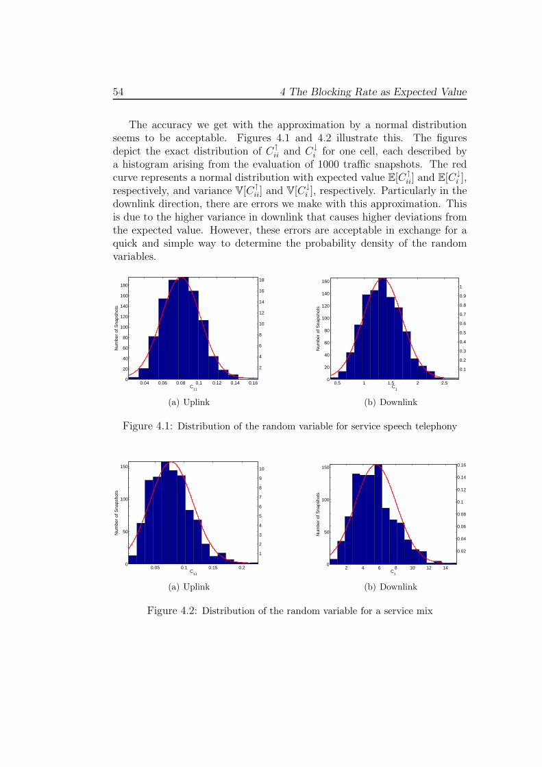
54 4 The Blocking Rate as Expected Value
The accuracy we get with the approximation by a normal distributionseems to be acceptable. Figures 4.1 and 4.2 illustrate this. The figuresdepict the exact distribution of C↑
ii and C↓i for one cell, each described by
a histogram arising from the evaluation of 1000 traffic snapshots. The redcurve represents a normal distribution with expected value E[C↑
ii] and E[C↓i ],
respectively, and variance V[C↑ii] and V[C↓
i ], respectively. Particularly in thedownlink direction, there are errors we make with this approximation. Thisis due to the higher variance in downlink that causes higher deviations fromthe expected value. However, these errors are acceptable in exchange for aquick and simple way to determine the probability density of the randomvariables.
0.04 0.06 0.08 0.1 0.12 0.14 0.160
20
40
60
80
100
120
140
160
180
C11
Num
ber
of S
naps
hots
2
4
6
8
10
12
14
16
18
(a) Uplink
0.5 1 1.5 2 2.50
20
40
60
80
100
120
140
160
C1
Num
ber
of S
naps
hots
0.1
0.2
0.3
0.4
0.5
0.6
0.7
0.8
0.9
1
(b) Downlink
Figure 4.1: Distribution of the random variable for service speech telephony
0.05 0.1 0.15 0.20
50
100
150
C11
Num
ber
of S
naps
hots
1
2
3
4
5
6
7
8
9
10
(a) Uplink
2 4 6 8 10 12 140
50
100
150
C1
Num
ber
of S
naps
hots
0.02
0.04
0.06
0.08
0.1
0.12
0.14
0.16
(b) Downlink
Figure 4.2: Distribution of the random variable for a service mix

5 Power Knapsack
An alternative approach of approximating the blocking rates of the cells ina UMTS radio network is discussed in this chapter. We understand thegiven task as a Knapsack problem. In such a problem, we are given a set ofelements, each with a certain weight and value. The task is to find a subsetout of the given set in a way that its total weight does not exceed a certainbound and that its accumulated value is at maximum.
In our case, we have a kind of fractional power knapsack. We make twocentral assumptions in this model:
(1) The power of the own antenna is at its maximum.
(2) We use constant estimates for the powers of the other antennas.
With these conditions, we are able to assign a specified weight to each mobilein our sector. This weight represents the power that would be received fromor consumed by the user if it was served under the above assumptions. Thebound in our Knapsack problem is the maximum power the antenna is able toreceive from or transmit on the dedicated channels. Due to the assumptionof compressible user demand (cf. Section 3.1.3) it is possible to “fill” ourpower knapsack until the bound is met exactly. The surplus is not served.Hence, the ratio of unserved user weight to the total weight of all mobilesin the sector represents the blocking rate. In our basic model, we assumethe power level of the considered antenna to be at its maximum if blockingoccurs. From this point of view, condition (1) is reasonable. We use theexpected coupling approach from Section 3.1.2 to assess the powers of theother base station antennas.
First, the method is introduced at a set of mobile stations given by a trafficsnapshot. Afterwards, we consider the distribution of the accumulated weightof all mobiles in the cell. This random variable is assumed to be normallydistributed as sum of many independent random variables. We determine theexpected value of the average blocking rate depending on the total weight ofall users in the cell.
55
56 5 Power Knapsack
5.1 Snapshot Based Derivation
This section derives the approach for a traffic snapshot. The basic idea can befound in [1], where it was introduced merely for the downlink direction. Thisthesis also covers the uplink afterwards and enhances the proposed model.
5.1.1 Downlink
For a base station antenna i ∈ N , the size of the power knapsack κ↓i is defined
as
κ↓i := pmax↓
i − p(c)i . (5.1)
This value represents the mentioned upper bound of our cell. We assume,that the present mobiles in cell i consume exactly this power. The totalaverage transmission power of antenna i allocated to the traffic on dedicatedchannels if all mobile stations in its sector are served reads as
∑
m∈Miα↓
m p↓im.
The value p↓im is the transmission power from antenna i to mobile m underthe condition that the antenna transmits at its maximum power level pmax↓
i
(assumption (1)). The power p↓im can be determined using the CIR targetequality introduced in (2.8). Due to assumptions (1) and (2), we obtain
µ↓m =
γ↓im p↓im
γ↓im ωm
(
pmax↓i − α↓
m p↓im
)
+∑
j 6=i γ↓jm p↓j + ηm
.
The powers p↓j for all j 6= i are the solutions of the system of equations (3.14)
using the expected coupling matrix. Solving the above equation for p↓imresults in
p↓im =l↓m
α↓m
(
ωm pmax↓i +
∑
j 6=i
γ↓jm
γ↓im
p↓j +ηm
γ↓im
)
. (5.2)
The downlink user load l↓m for mobile station m is defined by (3.6).In Section 2.5.3, we derived the condition for no blocking to occur in
cell i. With the definition (5.1) of κ↓i , the downlink inequality of (2.10) can
be transformed into∑
m∈Mi
α↓m p↓im ≤ κ↓
i . (5.3)
It is convenient to write this as
1
κ↓i
∑
m∈Mi
α↓m p↓im ≤ 1. (5.4)

5.1 Snapshot Based Derivation 57
The values α↓m p↓im are the weights of our Knapsack problem for each mobile
in the sector. We define the left hand side of inequality (5.4) as K↓i , that is,
K↓i :=
1
κ↓i
∑
m∈Mi
α↓m p↓im. (5.5)
This can be understood as the content that shall fit into the power knapsack.The variable K↓
i depends on the set of served mobile stations Mi since p↓immight be different for different users. The value K↓
i approximates the frac-tion of total available transmission power of antenna i spent on the trafficon dedicated channels. Inequality (5.4) states that blocking occurs if thisfraction is greater than one. That means, we “fill” our power knapsack withmobile weights α↓
m p↓im until the bound of one is reached exactly. In doingso, some of these weights might be taken fractionally. The (fractions of) userweights contributing to the excess are rejected. Therefore, the average down-link blocking rate b↓i of base station antenna i for the considered snapshot isgiven by
b↓i =
0 for K↓i ≤ 1
K↓i −1
K↓i
for K↓i > 1.
(5.6)
We verify this formula by showing that
b↓i = 1 − λ↓i .
The scaling factor λ↓i – introduced in Section 3.1.3 – is defined by:
λ↓i = min
{
1,pmax↓
i − p(c)i
C↓ii p
max↓i +
∑
j 6=i C↓ij p↓j + p
(η)i
}
. (5.7)
This formulation can be derived from (3.14) since we estimate the otherantennas’ powers p↓j , j 6= i (assumption (2)).
(i) In the case that K↓i ≤ 1, equation (5.3) holds. Substituting p↓im accor-
ding to (5.2) yields
∑
m∈Mi
l↓m
(
ωm pmax↓i +
∑
j 6=i
γ↓jm
γ↓im
p↓j +ηm
γ↓im
)
≤ κ↓i .
This is equivalent to
C↓ii p
max↓i +
∑
j 6=i
C↓ij p↓j + p
(η)i ≤ pmax↓
i − p(c)i .
Hence follows, that λ↓i = 1 and thus b↓i = 1 − λ↓
i .

58 5 Power Knapsack
(ii) In the case that K↓i > 1, it holds that
C↓ii p
max↓i +
∑
j 6=i
C↓ij p↓j + p
(η)i > pmax↓
i − p(c)i .
Therefore, λ↓i is assessed by
λ↓i =
pmax↓i − p
(c)i
C↓ii p
max↓i +
∑
j 6=i C↓ij p↓j + p
(η)i
.
For b↓i , we obtain
b↓i =K↓
i − 1
K↓i
= 1 −1
1
κ↓i
∑
m∈Miα↓
m p↓im
= 1 −κ↓
i
∑
m∈Mil↓m
(
ωm pmax↓i +
∑
j 6=i
γ↓jm
γ↓im
p↓j + ηm
γ↓im
)
= 1 −pmax↓
i − p(c)i
C↓ii p
max↓i +
∑
j 6=i C↓ij p↓j + p
(η)i
= 1 − λ↓i .
�
5.1.2 Uplink
In the uplink direction, a base station antenna does not only receive signalsfrom the mobile stations in the own sector. Instead, the reception powerof an antenna is composed of the received powers of all users in the entireplanning area. Depending on the attenuation factor from a mobile stationto the considered antenna, the strength of the incoming power varies. Weassume that the contributions of the other cells j 6= i are constant at theirexpected average values. That is,
∑
j 6=i
C↑ij p↑j = constant.
The matrix C↑ is the scaled, expected cell load coupling matrix. The scalingdescribes the blocking behavior of a cell. An antenna rejects users exceedingits power limits. In order to represent this functionality, the scaling has tobe involved. The maximum power antenna i can receive from the mobiles inthe own cell reads as
κ↑i = pmax↑
i −∑
j 6=i
C↑ij p↑j − ηi. (5.8)

5.1 Snapshot Based Derivation 59
This is the upper bound or size of our power knapsack.The total average reception power arising from all present users in the cell
if none of them is blocked is given by∑
m∈Miγ↑
mi α↑m p↑m. With condition (1),
we obtain from the CIR target equality (2.6):
p↑m =l↑m
γ↑mi α
↑m
pmax↑i . (5.9)
The situation that there is enough capacity to serve all users in cell i inuplink is characterized by
∑
m∈Mi
γ↑mi α
↑m p↑m ≤ κ↑
i . (5.10)
We transform this inequality into
1
κ↑i
∑
m∈Mi
γ↑mi α
↑m p↑m ≤ 1. (5.11)
The weights of our knapsack are the values γ↑mi α
↑m p↑m for each mobile station
in cell i. We define the fraction of total possible reception power at antenna istemming from the traffic on dedicated channels of the own cell by
K↑i :=
1
κ↑i
∑
m∈Mi
γ↑mi α
↑m p↑m. (5.12)
Due to inequality (5.11), we can “put” mobile powers into the power knapsackuntil we meet the upper bound of one exactly. That part of the total offeredmobile reception power K↑
i greater than one is rejected. Thus, for the averageblocking rate b↑i at base station antenna i in the given traffic snapshot holds:
b↑i =
0 for K↑i ≤ 1
K↑i −1
K↑i
for K↑i > 1.
(5.13)
We prove this formula by deriving that
b↑i = 1 − λ↑i .
If blocking occurs in cell i, that is, λ↑i < 1, it holds that
pmax↑i = C↑
ii λ↑i pmax↑
i +∑
j 6=i
C↑ij p↑j + ηi
due to (3.16). Hence, the scaling factor λ↑i is given by
λ↑i = min
{
1,pmax↑
i −∑
j 6=i C↑ij p↑j − ηi
C↑ii p
max↑i
}
. (5.14)
60 5 Power Knapsack
(i) Let K↑i ≤ 1 hold. That is, inequality (5.10) is satisfied. If we replace
p↑m according to (5.9), this results in
∑
m∈Mi
l↑m pmax↑i ≤ κ↑
i .
This can be written as
C↑ii p
max↑i ≤ pmax↑
i −∑
j 6=i
C↑ij p↑j − ηi.
Therefore, λ↑i = 1 and b↑i = 1 − λ↑
i .
(ii) In the case that K↑i > 1, it holds that
C↑ii p
max↑i > pmax↑
i −∑
j 6=i
C↑ij p↑j − ηi.
Hence follows, that
λ↑i =
pmax↑i −
∑
j 6=i C↑ij p↑j − ηi
C↑ii p
max↑i
.
For the average blocking rate b↑i , we receive
b↑i =K↑
i − 1
K↑i
= 1 −1
1
κ↑i
∑
m∈Miγ↑
mi α↑m p↑m
= 1 −κ↑
i∑
m∈Mil↑m pmax↑
i
= 1 −pmax↑
i −∑
j 6=i C↑ij p↑j − ηi
C↑ii p
max↑i
= 1 − λ↑i .
�
5.2 The Expected Power Knapsack
In this section, we understand the variables K↓i and K↑
i as realizations ofrandom variables. In this way, the proposed method can be generalized onthe basis of average traffic load distributions. The random variables aresupposed to follow a normal distribution because they are the sum of many

5.2 The Expected Power Knapsack 61
independent random variables. We determine the expected value of the ave-rage blocking rate depending on the scaled, accumulated user weight K↑
i
and K↓i , respectively. As in former chapters, we assume representative CIR
targets µ↓s, µ↑
s and transmit activity factors α↓s, α↑
s for every service s ∈ S.Moreover, the orthogonality factors ωp and noise ηp in downlink are location-
specific as well as the attenuation factors γ↓ip and γ↑
pi.
5.2.1 Downlink
We substitute p↓im according to (5.2) in the definition (5.5) of K↓i . This results
in
K↓i =
1
κ↓i
∑
m∈Mi
(
ωm pmax↓i +
∑
j 6=i
γ↓jm
γ↓im
p↓j +ηm
γ↓im
)
l↓m.
According to (5.4), there is no blocking in downlink at antenna i if
K↓i ≤ 1
holds. For K↓i > 1, the average blocking rate is determined by (5.6). Thus,
the expected value of the average blocking rate in cell i can be obtained by
E[b↓i ] =
∫ ∞
1
x − 1
xf ↓
i (x) dx. (5.15)
Here, f ↓i denotes the probability density function of K↓
i .
The random variable K↓i can be assumed to follow a normal distribution.
In fact, the limiting distribution as the number of pixels in the cell area |Ai|goes to infinity is not a normal distribution. The proof is the same as givenin Section 4.4.3 with
ls(p) =1
κ↓i
(
ωp pmax↓i +
∑
j 6=i
γ↓jp
γ↓ip
p↓j +ηp
γ↓ip
)
α↓s µ↓
s
1 + ωp α↓s µ↓
s
.
Nevertheless, the assumption is sensible for the same reasons as discussed inSection 4.4.4. In order to assess the probability density function f ↓
i of K↓i we
need to compute the expected value and variance of this random variable.The expected value of K↓
i is determined by
E[K↓i ] =
1
κ↓i
∫
p∈Ai
(
ωp pmax↓i +
∑
j 6=i
γ↓jp
γ↓ip
p↓j +ηp
γ↓ip
)
l↓p dp. (5.16)

62 5 Power Knapsack
Remember, that l↓p defined in (3.11) is the expected value of l↓m in position p.
The variance of K↓i satisfies
V[K↓i ] =
1
(κ↓i )
2
∫
p∈Ai
(
ωp pmax↓i +
∑
j 6=i
γ↓jp
γ↓ip
p↓j +ηp
γ↓ip
)2
V[l↓m(p)] dp. (5.17)
The user densities in each pixel follow a Poisson distribution and are inde-pendent (cf. Section 2.5.2). Therefore, the variance of the user number isequal to its expected value. The variance of l↓m at location p is given by
V[l↓m(p)] =∑
s∈S
(
α↓s µ↓
s
1 + ωp α↓s µ↓
s
)2
Ts(p). (5.18)
The effect of coupling can be included as described in Section 4.3 in orderto improve the estimates of the other antennas’ powers and thus to obtainmore accurate results.
5.2.2 Uplink
In the uplink direction, the realization of the random variable K↑i for a traffic
snapshot reads as
K↑i =
1
κ↑i
∑
m∈Mi
l↑m pmax↑i .
There are all users served in cell i if
K↑i ≤ 1
holds (cf. (5.11)). The expected value of the uplink blocking rate can begoverned by
E[b↑i ] =
∫ ∞
1
x − 1
xf ↑
i (x) dx (5.19)
in which f ↑i denotes the probability density function of K↑
i .
The random variable K↑i is assumed to be normally distributed. As in
the previous chapter, the Central Limit Theorem does not apply. This canbe proved in analogy to Section 4.4.3 with
ls(p) =pmax↑
i
κ↑i
α↑s µ↑
s
1 + α↑s µ↑
s
.

5.2 The Expected Power Knapsack 63
However, a justification for this assumption can be found in Section 4.4.4.The expected value of K↑
i satisfies the expression
E[K↑i ] =
pmax↑i
κ↑i
∫
p∈Ai
l↑p dp. (5.20)
The variance of this random variable is determined by
V[K↑i ] =
(pmax↑i )2
(κ↑i )
2
∫
p∈Ai
V [l↑m(p)] dp. (5.21)
Here, the variance of l↑m at location p is given by
V[l↑m(p)] =∑
s∈S
(
α↑s µ↑
s
1 + α↑s µ↑
s
)2
Ts(p). (5.22)
With E[K↑i ] and V[K↑
i ], the probability density function f ↑i of K↑
i is uniquelydetermined. For the uplink direction, the effect of coupling can be taken intoaccount as pointed out in Section 4.3.

64 5 Power Knapsack

6 Comparison of both Methods
A central question now is how both approaches are related with each other.In this chapter, we prove that the results of the introduced methods fromthe last two chapters are equal. The model from Chapter 4 is considered forthe general case of varying user load. As in the past chapters, the subscripti marks the cell whose blocking rate shall be assessed. The index j denotesother base station antennas.
6.1 Uplink
The first approach deals with the random variable
C↑ii :=
∑
m∈Mi
l↑m.
The expected average blocking rate is determined according to
E[b↑i ] =
∫ ∞
0
[1 − λ↑i (x)] f ↑
i (x) dx (6.1)
with λ↑i given by
λ↑i (x) =
min{
1,pmax↑i −
P
j 6=i C↑ij p
↑j−ηi
x pmax↑i
}
for x > 0
1 for x = 0.
The second model covers the random variable
K↑i :=
pmax↑i
κ↑i
∑
m∈Mi
l↑m.
The expected average blocking rate reads as
E[b↑i ] =
∫ ∞
1
x − 1
xf ↑
i (x) dx. (6.2)
65

66 6 Comparison of both Methods
When comparing both random variables, it is easy to see that
K↑i =
pmax↑i
κ↑i
C↑ii (6.3)
holds. For this reason, following equality is satisfied for all x ∈ R:
f ↑i (x) = f ↑
i
(
pmax↑i
κ↑i
x
)
. (6.4)
The average blocking rate b↑i (x) = 1−λ↑i (x) is zero for λ↑
i (x) = 1, that is, for
x ≤pmax↑
i −∑
j 6=i C↑ij p↑j − ηi
pmax↑i
=κ↑
i
pmax↑i
.
Therefore, (6.1) is equal to
E[b↑i ] =
∫ ∞
κ↑i
pmax↑i
[
1 −pmax↑
i −∑
j 6=i C↑ij p↑j − ηi
x pmax↑i
]
f ↑i (x) dx. (6.5)
We apply (6.4) to (6.5) and define y :=pmax↑i
κ↑i
x. This yields
E[b↑i ] =
∫ ∞
κ↑i
pmax↑i
[
1 −κ↑
i
x pmax↑i
]
f ↑i
(
pmax↑i
κ↑i
x
)
dx
=
∫ ∞
1
[
1 −1
y
]
f ↑i (y) dy = E[b↑i ].
6.2 Downlink
In the downlink direction, the first model considers the random variable
C↓i :=
∑
m∈Mi
(
ωm pmax↓i +
∑
j 6=i
γ↓jm
γ↓im
p↓j +ηm
γ↓im
)
l↓m
The average blocking rate is approximated by its expected value in followingway:
E[b↓i ] =
∫ ∞
0
[1 − λ↓i (x)] f ↓
i (x) dx. (6.6)

6.2 Downlink 67
The scaling factor λ↓i is assessed by
λ↓i (x) =
min{
1,pmax↓i −p
(c)i
x
}
for x > 0
1 for x = 0.
In the second approach, we define the random variable
K↓i :=
1
κ↓i
∑
m∈Mi
(
ωm pmax↓i +
∑
j 6=i
γ↓jm
γ↓im
p↓j +ηm
γ↓im
)
l↓m.
The expected average blocking rate is given by
E[b↓i ] =
∫ ∞
1
x − 1
xf ↓
i (x) dx. (6.7)
From the above representation of K↓i we derive
K↓i =
1
κ↓i
C↓i . (6.8)
Due to this, it holds that
f ↓i (x) = f ↓
i
(
x
κ↑i
)
(6.9)
for all x ∈ R. Because λ↓i (x) = 1 for
x ≤ pmax↓i − p
(c)i = κ↓
i ,
E[b↓i ] can be written as
E[b↓i ] =
∫ ∞
κ↓i
[
1 −pmax↓
i − p(c)i
x
]
f ↓i (x) dx. (6.10)
With (6.9) and y := x
κ↑i
, this can be transformed in following way:
E[b↓i ] =
∫ ∞
κ↓i
[
1 −κ↓
i
x
]
f ↓i
( x
κ↑i
)
dx
=
∫ ∞
1
[
1 −1
y
]
f ↓i (y) dy = E[b↓i ].
�

68 6 Comparison of both Methods
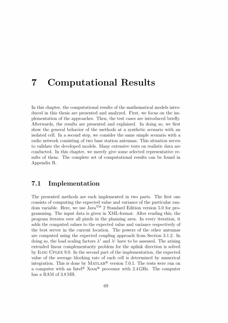
7 Computational Results
In this chapter, the computational results of the mathematical models intro-duced in this thesis are presented and analyzed. First, we focus on the im-plementation of the approaches. Then, the test cases are introduced briefly.Afterwards, the results are presented and explained. In doing so, we firstshow the general behavior of the methods at a synthetic scenario with anisolated cell. In a second step, we consider the same simple scenario with aradio network consisting of two base station antennas. This situation servesto validate the developed models. Many extensive tests on realistic data areconducted. In this chapter, we merely give some selected representative re-sults of them. The complete set of computational results can be found inAppendix B.
7.1 Implementation
The presented methods are each implemented in two parts. The first oneconsists of computing the expected value and variance of the particular ran-dom variable. Here, we use JavaTM 2 Standard Edition version 5.0 for pro-gramming. The input data is given in XML-format. After reading this, theprogram iterates over all pixels in the planning area. In every iteration, itadds the computed values to the expected value and variance respectively ofthe best server in the current location. The powers of the other antennasare computed using the expected coupling approach from Section 3.1.2. Indoing so, the load scaling factors λ↑ and λ↓ have to be assessed. The arisingextended linear complementarity problem for the uplink direction is solvedby Ilog Cplex 9.0. In the second part of the implementation, the expectedvalue of the average blocking rate of each cell is determined by numericalintegration. This is done by Matlab
R© version 7.0.1. The tests were run ona computer with an IntelR© XeonR© processor with 2.4GHz. The computerhas a RAM of 3.8MB.
69

70 7 Computational Results
7.2 Test Cases
In order to get a notion of how the methods work, the first test case is a syn-thetic scenario. We consider very simple network configurations. The firstradio network is an isolated cell. The second one consists of two base stationantennas. Besides those simple cases, the tests are conducted on realisticdatasets from the Momentum project [8, 18]. These scenarios comprise thedowntown regions of The Hague, Berlin and Lisbon. Complex propagationdata is given as well as non-homogeneous traffic distributions for differentservices. On each scenario, two different network designs are investigated.The smallest scenario is The Hague with 12 sites. This scenario covers anarea of 16 km2. The treated network configurations have 19 and 36 cells,respectively. The Berlin scenario extends over 56 km2 and has 65 sites. Thenetwork designs have each 122 sectors. The region covered by the Lisbonscenario is 21 km2 large. The scenario has 60 sites. One of the networks has128 cells, the other one 164. Moreover, the realistic Turin scenario developedwithin the Cost 273 Morans activity [19] is one of our test cases. Thecomplexity and scope of the data is equal to that of the data from the Mo-
mentum project. The network considered on the Turin scenario has 34 sitesand 103 cells.
In all covered radio networks, the maximum transmission power of abase station antenna is 20W. The downlink load limit is 70%. In the uplinkdirection, a maximum noise rise of around 3 dB is assumed. This correspondsto a load limit of 50%. We scale the traffic intensity with different factors(traffic scaling factors) in order to vary the amount of traffic. In doing so,we produce some overload. The considered service mixes vary, too. We testthe single-service case as well as service mixes. In the multi-service case,we conduct tests when merely circuit-switched (cs) services are included inthe scenarios like speech telephony and video telephony. Furthermore, amix of circuit- and packet-switched services is tested for all scenarios. Theessential average parameters for every service class are listed in Table 7.1 forthe downlink direction. The abbreviation R denotes the average bit rate ofthe service, α is its transmit activity factor and µ its average CIR target.
Service R [Kbps] α µ [dB]
Speech telephony 12.2 0.5 −15.90Video telephony 64.0 1.0 −11.56Data transmission 64.0 0.9 −10.95
Table 7.1: Average service parameters in downlink

7.3 Validation 71
We test two versions of each model. One takes the effect of coupling intoaccount according to (4.29) and (4.30), respectively (refined version), and onedoes not (simple version). The results are compared to those of Monte Carlosimulation on traffic snapshots introduced in Section 3.1.1. In [7] it is shownthat these results are a good approximation of results obtained by MonteCarlo simulation including a more extensive load analysis in each trial. Theerrorbars around the points belonging to these results represent the confi-dence intervals for a confidence level of 95% (cf. Section 3.2). Furthermore,the results of the approach using the expected coupling matrix from Sec-tion 3.1.2 are given. This model is the basis of the developed methods. Inthis way, the achieved improvement is revealed.
7.3 Validation
The synthetic scenario serves to validate the models introduced in this the-sis. For this reason, the complete curves of the blocking rate are plotteddepending on the different traffic scaling factors. This is done for every cellin logarithmic scale. The synthetic scenario is denoted by “Synth.” in thepictures. We additionally plot two dashed, magenta-colored lines in eachillustration marking the region of the blocking rate between 1 and 5%. Thisinterval is the most important for us. Blocking rates lower than 1% arenegligible. Those higher than 5% are not probable to occur in the networkdesigns we consider.
7.3.1 One Cell
In the case of an isolated cell there is no difference between the simple andthe refined version since there are no other antennas whose powers couldbe estimated. Figure 7.1 depicts the results for the isolated antenna of thesynthetic scenario in the case of the single service speech telephony in uplinkand downlink, respectively. We recognize, that all obtained values lie insidethe confidence intervals. Figure 7.2 illustrates the outcomes for the servicemix including merely the circuit-switched services. Figure 7.3 shows theresults for a general service mix. In both cases, almost all values lie insidethe confidence intervals. That is, the presented approaches deliver reasonableoutcomes for our purpose. Furthermore, the strong improvement comparedto the expected coupling method is noticeable. For low blocking rates, theresults of this method are zero and hence not depicted due to the logarithmicscale. Only in ranges over 5% the results of the expected coupling methodapproach the exact blocking rates.
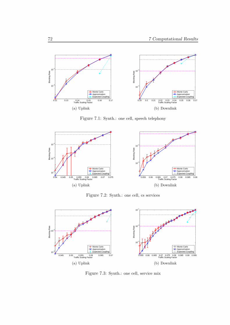
72 7 Computational Results
0.12 0.13 0.14 0.15 0.16 0.17
10−3
10−2
Traffic Scaling Factor
Blo
ckin
g R
ate
Monte CarloApproximationExpected Coupling
(a) Uplink
0.19 0.2 0.21 0.22 0.23 0.24 0.25 0.26 0.27
10−3
10−2
Traffic Scaling Factor
Blo
ckin
g R
ate
Monte CarloApproximationExpected Coupling
(b) Downlink
Figure 7.1: Synth.: one cell, speech telephony
0.04 0.045 0.05 0.055 0.06 0.065 0.07 0.075
10−4
10−3
10−2
Traffic Scaling Factor
Blo
ckin
g R
ate
Monte CarloApproximationExpected Coupling
(a) Uplink
0.055 0.06 0.065 0.07 0.075 0.08 0.085 0.09
10−3
10−2
Traffic Scaling Factor
Blo
ckin
g R
ate
Monte CarloApproximationExpected Coupling
(b) Downlink
Figure 7.2: Synth.: one cell, cs services
0.045 0.05 0.055 0.06 0.065 0.07
10−3
10−2
Traffic Scaling Factor
Blo
ckin
g R
ate
Monte CarloApproximationExpected Coupling
(a) Uplink
0.055 0.06 0.065 0.07 0.075 0.08 0.085 0.09 0.095
10−3
10−2
10−1
Traffic Scaling Factor
Blo
ckin
g R
ate
Monte CarloApproximationExpected Coupling
(b) Downlink
Figure 7.3: Synth.: one cell, service mix

7.3 Validation 73
7.3.2 Two Cells
For 100% speech telephony users, the results are shown in Figure 7.4 forboth cells in the uplink direction. The downlink is depicted in Figure 7.5. Ofcourse, the outcomes of the approaches are not as precise as for an isolatedantenna since more sources of estimation errors are involved, now. The Fi-gures 7.6–7.9 depict the results for different service mixes. All figures revealthat the blocking rate is systematically underestimated in low ranges under2–4%. We note that this underestimation is stronger in the simple version.The curve of the blocking rate of the simple variant approaches the curve ofthe exact blocking rate later than that of the refined alternative. Particularlyin the downlink direction, the results of the precise version are better. Thepowers of the other base station antennas are estimated higher in this variantand thus the blocking rate. In the uplink, the differences are very small andthus hardly to recognize in the diagrams. In general, the transmission powerof a cell is considerably higher than its reception power because the mobilestation antennas are much less powerful than the base station antennas.Therefore, the differences between the simple and the refined alternative arehigher in downlink.
This systematical estimation error is probably due to the fact that weestimate the powers of the other base station antennas by using the expectedcoupling model. As pointed out in Section 3.3, this approach tends to un-derestimate the average power of an antenna in low ranges. If the powers ofother antennas are estimated too low, the inter-cell interference in our sec-tor is underestimated. Thus, the blocking rate is underestimated, too. Thiscannot be compensated for completely by considering the effect of couplingin the refined versions of our methods. This enhancement determines anestimate for the average powers of the other antennas under the assumptionthat the power level of our antenna is at its maximum. However, the othercells’ powers are still underestimated compared to the exact powers condi-tioned to the situation when the power of our antenna is at its maximum.The reasons are the same as given in Section 3.3. Traffic snapshots withmore users than expected contribute above average to the exact power andblocking rate. These snapshots are as probable to occur in reality as trafficsnapshots with less users than expected. These effects of randomness areignored in the expected coupling approach. Furthermore, the assumption ofthe random variables of our methods being normally distributed is not valid(cf. Section 4.4). Hence, this approximation causes errors, too.

74 7 Computational Results
0.15 0.16 0.17 0.18 0.19 0.210
−4
10−3
10−2
Traffic Scaling Factor
Blo
ckin
g R
ate
Monte CarloSimple VersionRefined VersionExpected Coupling
(a) Cell 1
0.15 0.16 0.17 0.18 0.19
10−4
10−3
10−2
Traffic Scaling Factor
Blo
ckin
g R
ate
Monte CarloSimple VersionRefined VersionExpected Coupling
(b) Cell 2
Figure 7.4: Synth.: two cells, speech telephony, uplink
0.2 0.21 0.22 0.23 0.24 0.25 0.26 0.27
10−4
10−3
10−2
Traffic Scaling Factor
Blo
ckin
g R
ate
Monte CarloSimple VersionRefined VersionExpected Coupling
(a) Cell 1
0.22 0.23 0.24 0.25 0.26 0.27 0.28 0.29 0.3
10−3
10−2
Traffic Scaling Factor
Blo
ckin
g R
ate
Monte CarloSimple VersionRefined VersionExpected Coupling
(b) Cell 2
Figure 7.5: Synth.: two cells, speech telephony, downlink
0.05 0.055 0.06 0.065 0.07 0.075 0.08 0.085 0.09
10−4
10−3
10−2
Traffic Scaling Factor
Blo
ckin
g R
ate
Monte CarloSimple VersionRefined VersionExpected Coupling
(a) Cell 1
0.05 0.055 0.06 0.065 0.07 0.075 0.08 0.085
10−4
10−3
10−2
Traffic Scaling Factor
Blo
ckin
g R
ate
Monte CarloSimple VersionRefined VersionExpected Coupling
(b) Cell 2
Figure 7.6: Synth.: two cells, cs services, uplink

7.3 Validation 75
0.055 0.06 0.065 0.07 0.075 0.08 0.085 0.09
10−4
10−3
10−2
Traffic Scaling Factor
Blo
ckin
g R
ate
Monte CarloSimple VersionRefined VersionExpected Coupling
(a) Cell 1
0.06 0.065 0.07 0.075 0.08 0.085 0.09 0.095 0.110
−4
10−3
10−2
Traffic Scaling Factor
Blo
ckin
g R
ate
Monte CarloSimple VersionRefined VersionExpected Coupling
(b) Cell 2
Figure 7.7: Synth.: two cells, cs services, downlink
0.05 0.055 0.06 0.065 0.07 0.075 0.08
10−3
10−2
10−1
Traffic Scaling Factor
Blo
ckin
g R
ate
Monte CarloSimple VersionRefined VersionExpected Coupling
(a) Cell 1
0.05 0.055 0.06 0.065 0.07 0.075 0.08
10−3
10−2
10−1
Traffic Scaling Factor
Blo
ckin
g R
ate
Monte CarloSimple VersionRefined VersionExpected Coupling
(b) Cell 2
Figure 7.8: Synth.: two cells, service mix, uplink
0.06 0.065 0.07 0.075 0.08 0.085 0.09 0.095
10−4
10−3
10−2
10−1
Traffic Scaling Factor
Blo
ckin
g R
ate
Monte CarloSimple VersionRefined VersionExpected Coupling
(a) Cell 1
0.065 0.07 0.075 0.08 0.085 0.09 0.095 0.110
−4
10−3
10−2
10−1
Traffic Scaling Factor
Blo
ckin
g R
ate
Monte CarloSimple VersionRefined VersionExpected Coupling
(b) Cell 2
Figure 7.9: Synth.: two cells, service mix, downlink
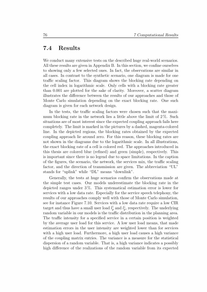
76 7 Computational Results
7.4 Results
We conduct many extensive tests on the described huge real-world scenarios.All these results are given in Appendix B. In this section, we confine ourselvesto showing only a few selected ones. In fact, the observations are similar inall cases. In contrast to the synthetic scenario, one diagram is made for onetraffic scaling factor. This diagram shows the blocking rate depending onthe cell index in logarithmic scale. Only cells with a blocking rate greaterthan 0.001 are plotted for the sake of clarity. Moreover, a scatter diagramillustrates the difference between the results of our approaches and those ofMonte Carlo simulation depending on the exact blocking rate. One suchdiagram is given for each network design.
In the tests, the traffic scaling factors were chosen such that the maxi-mum blocking rate in the network lies a little above the limit of 2%. Suchsituations are of most interest since the expected coupling approach fails herecompletely. The limit is marked in the pictures by a dashed, magenta-coloredline. In the depicted regions, the blocking rates obtained by the expectedcoupling approach lie around zero. For this reason, these blocking rates arenot shown in the diagrams due to the logarithmic scale. In all illustrations,the exact blocking rate of a cell is colored red. The approaches introduced inthis thesis are colored blue (refined) and green (simple), respectively. Thisis important since there is no legend due to space limitations. In the captionof the figures, the scenario, the network, the services mix, the traffic scalingfactor, and the direction of transmission are given. The abbreviation “UL”stands for “uplink” while “DL” means “downlink”.
Generally, the tests at huge scenarios confirm the observations made atthe simple test cases. Our models underestimate the blocking rate in thedepicted ranges under 3%. This systematical estimation error is lower forservices with a low data rate. Especially for the service speech telephony, theresults of our approaches comply well with those of Monte Carlo simulation,see for instance Figure 7.10. Services with a low data rate require a low CIRtarget and thus have a small user load l↑p and l↓p, respectively. The underlyingrandom variable in our models is the traffic distribution in the planning area.The traffic intensity for a specified service in a certain position is weightedby the average user load for this service. A low user load means, that madeestimation errors in the user intensity are weighted lower than for serviceswith a high user load. Furthermore, a high user load causes a high varianceof the coupling matrix entries. The variance is a measure for the statisticaldispersion of a random variable. That is, a high variance indicates a possiblyhigh difference of the realizations of the random variable from its expected
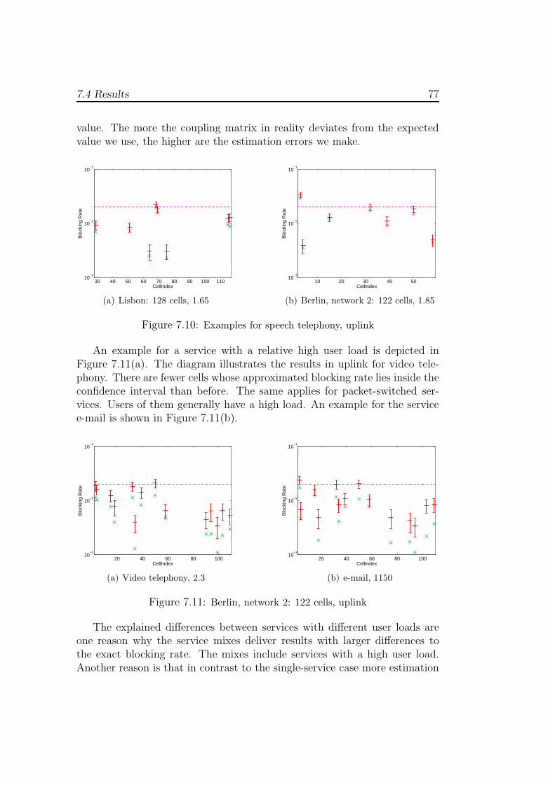
7.4 Results 77
value. The more the coupling matrix in reality deviates from the expectedvalue we use, the higher are the estimation errors we make.
30 40 50 60 70 80 90 100 11010
−3
10−2
10−1
CellIndex
Blo
ckin
g R
ate
(a) Lisbon: 128 cells, 1.65
10 20 30 40 5010
−3
10−2
10−1
CellIndexB
lock
ing
Rat
e
(b) Berlin, network 2: 122 cells, 1.85
Figure 7.10: Examples for speech telephony, uplink
An example for a service with a relative high user load is depicted inFigure 7.11(a). The diagram illustrates the results in uplink for video tele-phony. There are fewer cells whose approximated blocking rate lies inside theconfidence interval than before. The same applies for packet-switched ser-vices. Users of them generally have a high load. An example for the servicee-mail is shown in Figure 7.11(b).
20 40 60 80 10010
−3
10−2
10−1
CellIndex
Blo
ckin
g R
ate
(a) Video telephony, 2.3
20 40 60 80 10010
−3
10−2
10−1
CellIndex
Blo
ckin
g R
ate
(b) e-mail, 1150
Figure 7.11: Berlin, network 2: 122 cells, uplink
The explained differences between services with different user loads areone reason why the service mixes deliver results with larger differences tothe exact blocking rate. The mixes include services with a high user load.Another reason is that in contrast to the single-service case more estimation

78 7 Computational Results
errors are involved for several services. The errors made for each serviceare accumulated in this case. Examples are depicted in Figure 7.12. In allpresented figures, we see the difference between the simple and the refinedversion of our approaches. As in the synthetic scenario, the differences indownlink are much higher than in the uplink direction. In the uplink, theresults of both versions are roughly equal.
20 40 60 80 10010
−3
10−2
10−1
Cell Index
Blo
ckin
g R
ate
(a) Network 1, cs services, 0.58
20 40 60 80 100 12010
−3
10−2
10−1
Cell Index
Blo
ckin
g R
ate
(b) Network 2, service mix, 0.5
Figure 7.12: Berlin: 122 cells, different service mixes, downlink
Figure 7.13 depicts the scatter diagram for one network of the Berlinscenario in uplink. Figure 7.13(a) shows the entire diagram for all testedtraffic scaling factors. Figure 7.13(b) illustrates the extract marked by theblack rectangle in Figure 7.13(a). These diagrams visualize the differencebetween our refined methods and Monte Carlo simulation depending on theexact blocking rate. The values of all cells are plotted for all used trafficscaling factors and services. Each service is marked by a different color.The legend is merely given in Figure 7.13(a) due to space limitations inFigure 7.13(b). The different traffic scaling factors used explain the differentheights of the exact blocking rate for different service mixes.
These scatter diagrams show again that our approaches underestimate theblocking rate of most cells in low regions under around 5%. In higher rangesover approximately 10%, they usually overestimate the exact blocking rate.The reason is the same as for the underestimation explained in Section 7.3.2.We miscalculate the powers of the other antennas. The other cells’ powerstend to be overestimated by the expected coupling approach in high regions(cf. Section 3.3). Therefore, the inter-cell interference is overestimated andthus the blocking rate in our sector. The described estimation error has moreeffect on cells with high coupling to their neighbors.
Figure 7.14 shows the scatter diagram for the same network in downlink.We recognize that the blocking rate of most cells is underestimated under
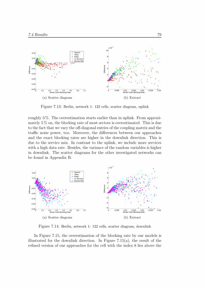
7.4 Results 79
0 0.1 0.2 0.3 0.4 0.5 0.6 0.7−0.05
−0.04
−0.03
−0.02
−0.01
0
0.01
0.02
Monte Carlo Blocking Rate
Diff
eren
ce
SpeechVideoEMailcs ServicesService Mix
(a) Scatter diagram
0 0.005 0.01 0.015 0.02 0.025 0.03
−2
0
2
4
6
8
10x 10
−3
Monte Carlo Blocking Rate
Diff
eren
ce
(b) Extract
Figure 7.13: Berlin, network 1: 122 cells, scatter diagram, uplink
roughly 3%. The overestimation starts earlier than in uplink. From approxi-mately 5% on, the blocking rate of most sectors is overestimated. This is dueto the fact that we vary the off-diagonal entries of the coupling matrix and thetraffic noise power, too. Moreover, the differences between our approachesand the exact blocking rates are higher in the downlink direction. This isdue to the service mix. In contrast to the uplink, we include more serviceswith a high data rate. Besides, the variance of the random variables is higherin downlink. The scatter diagrams for the other investigated networks canbe found in Appendix B.
0 0.1 0.2 0.3 0.4 0.5 0.6 0.7−0.05
−0.04
−0.03
−0.02
−0.01
0
0.01
0.02
Monte Carlo Blocking Rate
Diff
eren
ce
SpeechVideoEMailcs ServicesService Mix
(a) Scatter diagram
0 0.005 0.01 0.015 0.02 0.025 0.03−6
−4
−2
0
2
4
6
8
x 10−3
Monte Carlo Blocking Rate
Diff
eren
ce
(b) Extract
Figure 7.14: Berlin, network 1: 122 cells, scatter diagram, downlink
In Figure 7.15, the overestimation of the blocking rate by our models isillustrated for the downlink direction. In Figure 7.15(a), the result of therefined version of our approaches for the cell with the index 8 lies above the

80 7 Computational Results
confidence interval. Actually, such a strong overestimation in these low re-gions is exceptional. This is the only case of all conducted tests in which theblocking rate lies above the confidence interval for a cell with an exact block-ing rate under 2%. In other cases of overestimation in these low regions, theapproximation lies inside the confidence interval as shown in Figure 7.15(b)for the cell with the index 90.
4 5 6 7 8 9 10 1110
−3
10−2
10−1
Cell Index
Blo
ckin
g R
ate
(a) The Hague: 19 cells, speech tele-phony, 6
20 40 60 80 10010
−3
10−2
10−1
Cell Index
Blo
ckin
g R
ate
(b) Berlin, network 1: 122 cells, videotelephony, 3.5
Figure 7.15: Examples for overestimation, downlink
7.4.1 Running Time
The average running times for the simple versions of our methods are listedin Table 7.2. Those of the refined variants are given in Table 7.3. The totalrunning time is broken down into the two parts of implementation describedin Section 7.1. The entries in the column “Part I” specify the time needed tocompute the expected value and variance of the random variables includingthe time for solving the modified equation systems (4.29) and (4.30) in therefined version. The column “Intg” shows the running time for numericalintegration in the second part. All the times are given in seconds. Thecolumns with title “I” each refer to the first model introduced in Chapter 4.The heading “II” stands for the second method given in Chapter 5.
The first approach is a few seconds quicker in the first part of the imple-mentation. The reason is the computational complexity of calculating theknapsack size κ↑
i in uplink in the second model. For assessing this value forevery cell, the entries of the coupling matrix are summed up for each row.This causes additional computational effort of quadratic size in the numberof cells. However, the first approach takes on average more time for the nu-merical integration in the second part of the implementation. The reason is

7.4 Results 81
Number Part I Intg TotalScenario
of Cells I [s] II [s] I [s] II [s] I [s] II [s]
19 34.00 37.46 1.61 0.50 35.16 37.96The Hague
36 32.92 34.26 1.64 0.43 34.56 34.69Turin 103 53.93 64.90 5.71 1.34 59.64 66.24Berlin, network 1 122 41.11 47.21 8.27 2.34 49.38 49.55Berlin, network 2 122 39.79 51.97 7.57 2.08 47.36 54.05
128 67.73 72.65 7.59 2.11 75.32 74.76Lisbon
164 61.15 65.16 6.94 1.66 68.09 66.82
Table 7.2: Average running times of the simple versions
that the computation of λ↑i in the first model is more complex than calcu-
lating x−1x
in the second method. Again, the entries of the uplink couplingmatrix are summed up for every row. The relative differences between themodels are smaller in the first part of the implementation. This is probablydue to the use of a different program for each part. Altogether, the averagetotal running time of both approaches is about the same.
Number Part I Intg TotalScenario
of Cells I [s] II [s] I [s] II [s] I [s] II [s]
19 35.50 39.05 1.60 0.48 37.10 39.53The Hague
36 38.53 43.04 1.63 0.41 40.16 43.45Turin 103 71.10 78.35 5.76 1.35 76.86 79.70Berlin, network 1 122 73.07 75.92 8.31 2.31 81.38 78.23Berlin, network 2 122 72.81 80.12 7.42 2.10 80.23 82.22
128 102.79 107.87 7.64 2.10 110.43 109.97Lisbon
164 156.58 158.44 6.91 1.72 163.49 160.16
Table 7.3: Average running times of the refined versions
For small scenarios, like The Hague, the difference between the simpleand the refined versions of our approaches is negligible. By contrast, inlarger scenarios solving the modified equation system takes approximatelyjust as long as computing the expected value and variance of the randomvariables. The time for numerical integration is only a few seconds even formany cells. This time is equal in both versions.
In Table 7.4, the average running times of the refined version of theapproach from Chapter 5 are compared to those of Monte Carlo simulation.

82 7 Computational Results
The times are given in seconds. During Monte Carlo simulation, we evaluate1000 traffic snapshots for each scenario by using the method introduced inSection 3.1.1. This analysis is implemented in JavaTM 2 Standard Editionversion 5.0, too. The extended linear complementarity problem arising bythe computation of the load scaling factors λ↑ in uplink is again solved byIlog Cplex 9.0. Besides the given time for computing the blocking rates,the time for creating the traffic snapshots has to be taken into account. Thisissue is not considered here.
Number Monte Model IIScenario
of Cells Carlo [s] [s]
19 612 40The Hague
36 765 44Turin 103 4864 80Berlin, network 1 122 3680 78Berlin, network 2 122 3680 82
128 4843 110Lisbon
164 9914 160
Table 7.4: Comparison of the average running times
7.5 Conclusions
In order to find a compromise between accuracy and complexity, we do notconsider the complete underlying system in full detail. The powers of theother antennas in the radio network are estimated by average values. More-over, we assume the random variables to be normally distributed. Thesesimplifications cause systematical estimation errors.
In general, these errors are similar to those of the basic expected couplingapproach but they are considerably lower. In low regions under approxi-mately 3–5%, the developed approaches underestimate the blocking rate. Inhigher ranges over roughly 5–10%, our methods tend to overestimate theblocking rate. However, these estimation errors lie in an acceptable range.Moreover, the average running times of the developed models are very short.Depending on the frequency of utilization during optimization we can preferthe more precise variant or the simple alternative which is about twice asquick. In the uplink, the results of both versions differ hardly from eachother. In the downlink, the refined version yields better results. The totalaverage running times of both proposed approaches are approximately equal.

7.5 Conclusions 83
Altogether, we recognize that the developed models approximate theblocking rates in a UMTS radio network very well. The presented compu-tational results confirm this statement. They reveal that we have advancedthe basic approach immensely. A further success is that our approaches arevery quick compared to the complexity of Monte Carlo simulation. That is,we found a trade-off between accuracy and computational effort. In conclu-sion, the methods introduced in this thesis are very efficient. We reached thegoal to develop a model having about the complexity of the expected coup-ling approach on the one hand and being about as precise as Monte Carlosimulation on the other hand.

84 7 Computational Results

8 Summary and Outlook
The goal of this thesis was to develop a mathematical model to efficientlyapproximate the blocking rates of the cells in a UMTS radio network. Theblocking rate denotes the fraction of unserved users due to limited radioresources at a base station antenna. This rate is an important criterion toevaluate the quality of a radio network design. So far, no adequate methodwas known, however, that is able to predict the average blocking rate quicklyand reliably. The difficulty is that the capacity of a UMTS radio cell varies.
In this thesis, two approaches were proposed to approximate the block-ing rates in UMTS radio networks. These methods are based on an existingmodel. In the first method, the inaccuracies of this existing approach were re-duced by computing the expected value of the average blocking rate depend-ing on the interference of the own cell. In the second method, the problemwas understood as a kind of fractional Knapsack problem. We considered thedistribution of the total weight of all users in the radio cell. Depending onthis accumulated weight, we determined the expected value of the averageblocking rate. In both approaches, the interference of the other radio cellswas estimated by average values. These estimates were stated more precisely,however, at the cost of complexity. Moreover, we derived analytically thatthe results of both models are equal.
Extensive computational tests revealed that we found a very good com-promise between accuracy and complexity with the developed methods. Thecharacteristics of the basic model are still weakly present. That is, in lowranges the blocking rate is a little underestimated and in higher regionslightly overestimated. However, in contrast to the situation before these sys-tematical estimation errors lie inside acceptable bounds. The computationalcomplexity of both introduced approaches is equal. In contrast to existingmethods with comparable accuracy, the average running times are extremelyshort.
The small estimation errors could be reduced by finding more precise es-timates of the other base station antennas’ powers. So far, we estimatedthem by average values, which produce little errors. Another simplification
85
86 8 Summary and Outlook
we made in our methods is that we assumed the considered random vari-ables to be normally distributed. We proved that this assumption does nothold. A more accurate characterization of the distribution of the randomvariables with low computational effort could improve our results. Further-more, the proposed model could be enhanced by including soft handover andby combining the uplink and the downlink direction instead of treating themindependently.

A Notation
Symbol Meaning
A Planning areaAi Cell area (best server area) of base station antenna ip Location in the planning aread Dimension of the planning area
N Set of base station antennas (cells) in the radio networki, j Base station antennas
M Set of mobilesMi Set of mobiles served by base station antenna im Mobile
S Set of servicess Service
Ts Average spatial traffic distribution of service sTs(p) Average traffic intensity of service s at location pλd d-dimensional Lebesgue-Measurefs User density of service s
p↑m Uplink transmission power from mobile m
p↓im Downlink transmission power from antenna i to mobile m
p(c)i Constant power of base station antenna i
p↑i Total average reception power at base station antenna i
p↓i Total average transmission power of base station antenna i
pmax↑i Maximum total reception power at base station antenna i
pmax↓i Maximum total transmission power of base station antenna i
87

88 A Notation
γ↑mi Uplink attenuation factor between mobile m and antenna i
γ↓im Downlink attenuation factor between antenna i and mobile m
α↑m, α↓
m Uplink/downlink transmit activity factor of mobile mµ↑
m, µ↓m Uplink/downlink CIR target of mobile m
ηi, ηm Noise at base station antenna i/mobile mωm Orthogonality factor of mobile ml↑m, l↓m Uplink/downlink user load of mobile m
γ↑pi Uplink attenuation factor between location p and antenna i
γ↓ip Downlink attenuation factor between antenna i and location p
α↑s, α↓
s Uplink/downlink transmit activity factor of service sµ↑
s, µ↓s Uplink/downlink CIR target of service s
ηp Noise at location pωp Orthogonality factor in location pl↑p, l
↓p Expected uplink/downlink user load in location p
C↑, C↓ Uplink/downlink cell load coupling matrixC↑, C↓ Expected uplink/downlink cell load coupling matrix
C↑, C↓ Scaled uplink/downlink cell load coupling matrix
p(η)i Traffic noise power at base station antenna i
p(η)i Expected traffic noise power at base station antenna i
p(η)i Scaled traffic noise power at base station antenna i
λ↑i , λ↓
i Scaling factor in uplink/downlink for cell i
p↑i Total average reception power at base station antenna i(solution of the scaled uplink equation system)
p↓i Total average transmission power of base station antenna i(solution of the scaled downlink equation system)
P(A) Probability of event AE[X] Expected value of random variable XV[X] Variance of random variable X
Tp Average traffic intensity at location p (single service case)Ti Average traffic intensity in cell iPTi
(n) Probability for n users in cell i
b↑i , b↓i Average uplink/downlink blocking rate of cell i (according toChapter 4)

89
nmax↑i Capacity of cell i in uplink
nmax↓i Capacity of cell i in downlink
l↑i , l↓i Average uplink/downlink load for a user in cell iM Set of mobility typesPp(m) Probability of mobility type m at location p
C↓i Random variable related to cell i in downlink
c↓im/c↓ip Constant factor for mobile m/pixel p in cell i in downlink
f ↑i , f ↓
i Probability density function of C↑ii/C
↓ii or C↓
i
Xkp Random variable for step k ∈ N and pixel p given by a tri-angular array {Xkp, p = 1, . . . , nk : nk ∈ N}
k Row index in the triangular arraynk Number of random variables Xkp in the kth row of the triangu-
lar arrayµkp Expected value of the random variable Xkp
σ2kp Variance of the random variable Xkp
Xk Sum of the random variables Xkp, p = 1, . . . , nk in the kth step
A(k)i Set of pixels in the cell area of base station antenna i in the kth
step
ls(p) Constant factor for service s in position pms(p) Number of mobile stations of service s in position pYp Random variable in pixel pYi Sum of the random variables Yp over all p ∈ Ai
µp Expected value of the random variable Yp
σ2p Variance of the random variable Yp
s2k Sum of the variances σ2
p over all p = 1, . . . , nk
li Upper bound of ls(p) in cell i
li Lower bound of ls(p) in cell iωi Lower bound of ωp in cell i
γ↓i Lower bound of γ↓
ip
ηi Upper bound of ηp in cell ip⋆ Pixel in the cell area of antenna i
κ↑i , κ↓
i Size of the uplink/downlink power knapsack of cell i
b↑i , b↓i Average uplink/downlink blocking rate of cell i (according toChapter 5)

90 A Notation
K↑i , K↓
i Random variable representing the offer for the power knapsackof cell i in uplink/downlink
f ↑i , f ↓
i Probability density function of K↑i /K↓
i
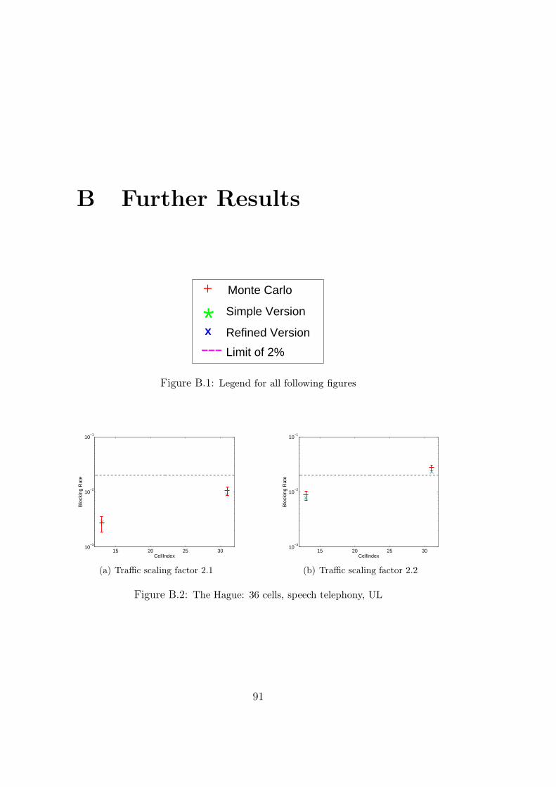
B Further Results
* Simple Version
Refined Versionx
+ Monte Carlo
Limit of 2%−−−
Figure B.1: Legend for all following figures
15 20 25 3010
−3
10−2
10−1
CellIndex
Blo
ckin
g R
ate
(a) Traffic scaling factor 2.1
15 20 25 3010
−3
10−2
10−1
CellIndex
Blo
ckin
g R
ate
(b) Traffic scaling factor 2.2
Figure B.2: The Hague: 36 cells, speech telephony, UL
91

92 B Further Results
12 13 14 15 16 17 18 1910
−3
10−2
10−1
Cell Index
Blo
ckin
g R
ate
(a) Traffic scaling factor 4.4
12 13 14 15 16 17 18 1910
−3
10−2
10−1
Cell Index
Blo
ckin
g R
ate
(b) Traffic scaling factor 4.6
Figure B.3: The Hague: 36 cells, speech telephony, DL
15 20 25 3010
−3
10−2
10−1
CellIndex
Blo
ckin
g R
ate
(a) Traffic scaling factor 1.2, UL
12 13 14 15 16 17 18 19 20 2110
−3
10−2
10−1
Cell Index
Blo
ckin
g R
ate
(b) Traffic scaling factor 0.8, DL
Figure B.4: The Hague: 36 cells, cs services
0 2 4 6 8 10 12 14 1610
−3
10−2
10−1
CellIndex
Blo
ckin
g R
ate
(a) Traffic scaling factor 2.55
0 2 4 6 8 10 12 14 1610
−3
10−2
10−1
CellIndex
Blo
ckin
g R
ate
(b) Traffic scaling factor 2.65
Figure B.5: The Hague: 19 cells, speech telephony, UL

93
4 5 6 7 8 9 10 1110
−3
10−2
10−1
Cell Index
Blo
ckin
g R
ate
Figure B.6: The Hague: 19 cells, speech telephony, traffic scaling 5.8, DL
0 2 4 6 8 10 12 14 1610
−3
10−2
10−1
CellIndex
Blo
ckin
g R
ate
(a) Traffic scaling factor 1.4
0 5 10 1510
−3
10−2
10−1
CellIndex
Blo
ckin
g R
ate
(b) Traffic scaling factor 1.5
Figure B.7: The Hague: 19 cells, cs services, UL
4 5 6 7 8 9 10 1110
−3
10−2
10−1
Cell Index
Blo
ckin
g R
ate
(a) Traffic scaling factor 0.9
2 4 6 8 1010
−3
10−2
10−1
Cell Index
Blo
ckin
g R
ate
(b) Traffic scaling factor 1.0
Figure B.8: The Hague: 19 cells, cs services, DL

94 B Further Results
10 20 30 40 5010
−3
10−2
10−1
CellIndex
Blo
ckin
g R
ate
(a) Traffic scaling factor 1.8
10 20 30 40 5010
−3
10−2
10−1
CellIndex
Blo
ckin
g R
ate
(b) Traffic scaling factor 1.85
Figure B.9: Berlin, network 1: 122 cells, speech telephony, UL
10 20 30 40 50 60 70 80 9010
−3
10−2
10−1
Cell Index
Blo
ckin
g R
ate
(a) Traffic scaling factor 3.3
10 20 30 40 50 60 70 80 9010
−3
10−2
10−1
Cell Index
Blo
ckin
g R
ate
(b) Traffic scaling factor 3.4
Figure B.10: Berlin, network 1: 122 cells speech telephony, DL
10 20 30 40 50 60 70 80 9010
−3
10−2
10−1
CellIndex
Blo
ckin
g R
ate
(a) Traffic scaling factor 2.2
20 40 60 80 10010
−3
10−2
10−1
CellIndex
Blo
ckin
g R
ate
(b) Traffic scaling factor 2.4
Figure B.11: Berlin, network 1: 122 cells, video telephony, UL
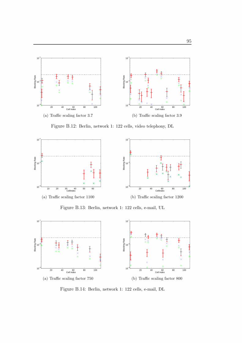
95
20 40 60 80 10010
−3
10−2
10−1
Cell Index
Blo
ckin
g R
ate
(a) Traffic scaling factor 3.7
20 40 60 80 10010
−3
10−2
10−1
Cell Index
Blo
ckin
g R
ate
(b) Traffic scaling factor 3.9
Figure B.12: Berlin, network 1: 122 cells, video telephony, DL
10 20 30 40 50 6010
−3
10−2
10−1
CellIndex
Blo
ckin
g R
ate
(a) Traffic scaling factor 1100
20 40 60 80 10010
−3
10−2
10−1
CellIndex
Blo
ckin
g R
ate
(b) Traffic scaling factor 1200
Figure B.13: Berlin, network 1: 122 cells, e-mail, UL
20 40 60 80 10010
−3
10−2
10−1
Cell Index
Blo
ckin
g R
ate
(a) Traffic scaling factor 750
20 40 60 80 10010
−3
10−2
10−1
Cell Index
Blo
ckin
g R
ate
(b) Traffic scaling factor 800
Figure B.14: Berlin, network 1: 122 cells, e-mail, DL

96 B Further Results
10 20 30 40 50 60 70 80 9010
−3
10−2
10−1
CellIndex
Blo
ckin
g R
ate
(a) Traffic scaling factor 1.0
10 20 30 40 50 60 70 80 9010
−3
10−2
10−1
CellIndex
Blo
ckin
g R
ate
(b) Traffic scaling factor 1.05
Figure B.15: Berlin, network 1: 122 cells, cs services, UL
20 40 60 80 10010
−3
10−2
10−1
Cell Index
Blo
ckin
g R
ate
Figure B.16: Berlin, network 1: 122 cells, cs services, 0.56, DL
10 20 30 40 50 60 70 80 9010
−3
10−2
10−1
CellIndex
Blo
ckin
g R
ate
(a) Traffic scaling factor 1.0
10 20 30 40 50 60 70 80 9010
−3
10−2
10−1
CellIndex
Blo
ckin
g R
ate
(b) Traffic scaling factor 1.05
Figure B.17: Berlin, network 1: 122 cells, service mix, UL

97
20 40 60 80 10010
−3
10−2
10−1
Cell Index
Blo
ckin
g R
ate
(a) Traffic scaling factor 0.52
20 40 60 80 10010
−3
10−2
10−1
Cell Index
Blo
ckin
g R
ate
(b) Traffic scaling factor 0.54
Figure B.18: Berlin, network 1: 122 cells, service mix, DL
10 20 30 40 5010
−3
10−2
10−1
CellIndex
Blo
ckin
g R
ate
Figure B.19: Berlin, network 2: 122 cells, speech telephony, 1.8, UL
10 20 30 40 5010
−3
10−2
10−1
Cell Index
Blo
ckin
g R
ate
(a) Traffic scaling factor 3.0
10 20 30 40 5010
−3
10−2
10−1
Cell Index
Blo
ckin
g R
ate
(b) Traffic scaling factor 3.05
Figure B.20: Berlin, network 2: 122 cells, speech telephony, DL
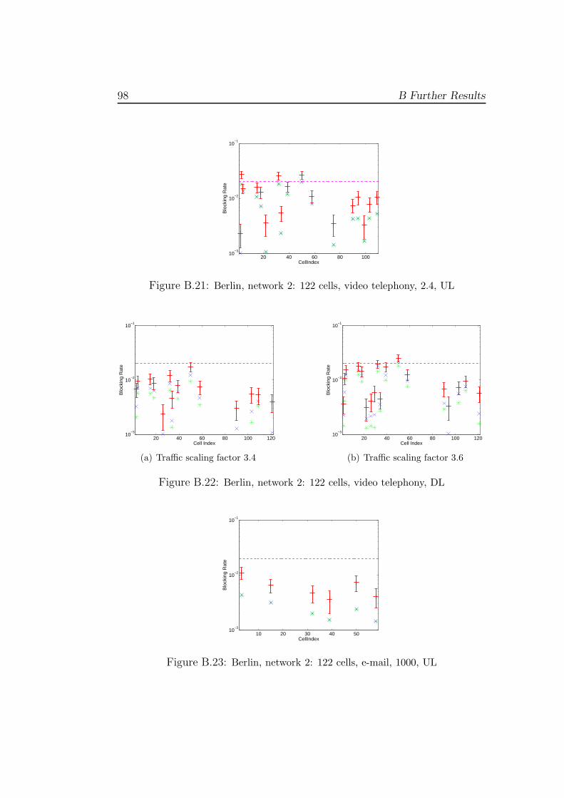
98 B Further Results
20 40 60 80 10010
−3
10−2
10−1
CellIndex
Blo
ckin
g R
ate
Figure B.21: Berlin, network 2: 122 cells, video telephony, 2.4, UL
20 40 60 80 100 12010
−3
10−2
10−1
Cell Index
Blo
ckin
g R
ate
(a) Traffic scaling factor 3.4
20 40 60 80 100 12010
−3
10−2
10−1
Cell Index
Blo
ckin
g R
ate
(b) Traffic scaling factor 3.6
Figure B.22: Berlin, network 2: 122 cells, video telephony, DL
10 20 30 40 5010
−3
10−2
10−1
CellIndex
Blo
ckin
g R
ate
Figure B.23: Berlin, network 2: 122 cells, e-mail, 1000, UL

99
20 40 60 80 10010
−3
10−2
10−1
Cell Index
Blo
ckin
g R
ate
(a) Traffic scaling factor 650
20 40 60 80 10010
−3
10−2
10−1
Cell Index
Blo
ckin
g R
ate
(b) Traffic scaling factor 700
Figure B.24: Berlin, network 2: 122 cells, e-mail, DL
20 40 60 80 10010
−3
10−2
10−1
CellIndex
Blo
ckin
g R
ate
(a) Traffic scaling factor 1.0
20 40 60 80 10010
−3
10−2
10−1
CellIndex
Blo
ckin
g R
ate
(b) Traffic scaling factor 1.05
Figure B.25: Berlin, network 2: 122 cells, cs services, UL
20 40 60 80 100 12010
−3
10−2
10−1
Cell Index
Blo
ckin
g R
ate
(a) Traffic scaling factor 0.52
20 40 60 80 100 12010
−3
10−2
10−1
Cell Index
Blo
ckin
g R
ate
(b) Traffic scaling factor 0.54
Figure B.26: Berlin, network 2: 122 cells, cs services, DL

100 B Further Results
10 20 30 40 5010
−3
10−2
10−1
CellIndex
Blo
ckin
g R
ate
(a) Traffic scaling factor 0.95
20 40 60 80 10010
−3
10−2
10−1
CellIndex
Blo
ckin
g R
ate
(b) Traffic scaling factor 1.0
Figure B.27: Berlin, network 2: 122 cells, service mix, UL
20 40 60 80 100 12010
−3
10−2
10−1
Cell Index
Blo
ckin
g R
ate
Figure B.28: Berlin, network 2: 122 cells, service mix, 0.48, DL
80 90 100 110 120 130 140 15010
−3
10−2
10−1
CellIndex
Blo
ckin
g R
ate
(a) Traffic scaling factor 1.35, UL
80 90 100 110 120 130 140 15010
−3
10−2
10−1
Cell Index
Blo
ckin
g R
ate
(b) Traffic scaling factor 2.05, DL
Figure B.29: Lisbon: 164 cells, speech telephony

101
80 90 100 110 120 130 140 15010
−3
10−2
10−1
CellIndex
Blo
ckin
g R
ate
(a) Traffic scaling factor 750
80 90 100 110 120 130 140 15010
−3
10−2
10−1
CellIndex
Blo
ckin
g R
ate
(b) Traffic scaling factor 850
Figure B.30: Lisbon: 164 cells, e-mail, UL
20 40 60 80 100 120 14010
−3
10−2
10−1
Cell Index
Blo
ckin
g R
ate
(a) Traffic scaling factor 475
20 40 60 80 100 120 14010
−3
10−2
10−1
Cell Index
Blo
ckin
g R
ate
(b) Traffic scaling factor 500
Figure B.31: Lisbon: 164 cells, e-mail, DL
80 90 100 110 120 130 140 15010
−3
10−2
10−1
CellIndex
Blo
ckin
g R
ate
(a) Traffic scaling factor 0.72
80 90 100 110 120 130 140 15010
−3
10−2
10−1
CellIndex
Blo
ckin
g R
ate
(b) Traffic scaling factor 0.74
Figure B.32: Lisbon: 164 cells, cs services, UL

102 B Further Results
20 40 60 80 100 120 14010
−3
10−2
10−1
Cell Index
Blo
ckin
g R
ate
(a) Traffic scaling factor 0.34
20 40 60 80 100 120 14010
−3
10−2
10−1
Cell Index
Blo
ckin
g R
ate
(b) Traffic scaling factor 0.36
Figure B.33: Lisbon: 164 cells, cs services, DL
80 90 100 110 120 130 140 15010
−3
10−2
10−1
CellIndex
Blo
ckin
g R
ate
(a) Traffic scaling factor 0.68
80 90 100 110 120 130 140 15010
−3
10−2
10−1
CellIndex
Blo
ckin
g R
ate
(b) Traffic scaling factor 0.74
Figure B.34: Lisbon: 164 cells, service mix, UL
20 40 60 80 100 120 14010
−3
10−2
10−1
Cell Index
Blo
ckin
g R
ate
(a) Traffic scaling factor 0.3
20 40 60 80 100 120 14010
−3
10−2
10−1
Cell Index
Blo
ckin
g R
ate
(b) Traffic scaling factor 0.32
Figure B.35: Lisbon: 164 cells, service mix, DL

103
30 40 50 60 70 80 90 100 11010
−3
10−2
10−1
CellIndex
Blo
ckin
g R
ate
Figure B.36: Lisbon: 128 cells, speech telephony, 1.6, UL
50 60 70 80 90 100 11010
−3
10−2
10−1
Cell Index
Blo
ckin
g R
ate
(a) Traffic scaling factor 2.5
30 40 50 60 70 80 90 100 11010
−3
10−2
10−1
Cell Index
Blo
ckin
g R
ate
(b) Traffic scaling factor 2.6
Figure B.37: Lisbon: 128 cells, speech telephony, DL
30 40 50 60 70 80 90 100 11010
−3
10−2
10−1
Cell Index
Blo
ckin
g R
ate
(a) Traffic scaling factor 575
30 40 50 60 70 80 90 100 11010
−3
10−2
10−1
Cell Index
Blo
ckin
g R
ate
(b) Traffic scaling factor 600
Figure B.38: Lisbon: 128 cells, e-mail, DL

104 B Further Results
30 40 50 60 70 80 90 100 11010
−3
10−2
10−1
CellIndex
Blo
ckin
g R
ate
(a) Traffic scaling factor 0.85
30 40 50 60 70 80 90 100 11010
−3
10−2
10−1
CellIndex
Blo
ckin
g R
ate
(b) Traffic scaling factor 0.9
Figure B.39: Lisbon: 128 cells, cs services, UL
30 40 50 60 70 80 90 100 11010
−3
10−2
10−1
Cell Index
Blo
ckin
g R
ate
(a) Traffic scaling factor 0.42
30 40 50 60 70 80 90 100 11010
−3
10−2
10−1
Cell Index
Blo
ckin
g R
ate
(b) Traffic scaling factor 0.43
Figure B.40: Lisbon: 128 cells, cs services, DL
30 40 50 60 70 80 90 100 11010
−3
10−2
10−1
CellIndex
Blo
ckin
g R
ate
(a) Traffic scaling factor 0.88
30 40 50 60 70 80 90 100 11010
−3
10−2
10−1
CellIndex
Blo
ckin
g R
ate
(b) Traffic scaling factor 0.9
Figure B.41: Lisbon: 128 cells, service mix, UL

105
30 40 50 60 70 80 90 100 11010
−3
10−2
10−1
Cell Index
Blo
ckin
g R
ate
(a) Traffic scaling factor 0.4
20 40 60 80 10010
−3
10−2
10−1
Cell Index
Blo
ckin
g R
ate
(b) Traffic scaling factor 0.42
Figure B.42: Lisbon: 128 cells, service mix, DL
20 30 40 50 60 70 80 90 10010
−3
10−2
10−1
CellIndex
Blo
ckin
g R
ate
(a) Traffic scaling factor 3.2
20 30 40 50 60 70 80 90 10010
−3
10−2
10−1
CellIndex
Blo
ckin
g R
ate
(b) Traffic scaling factor 3.3
Figure B.43: Turin: 103 cells, service mix, UL
20 30 40 50 60 70 80 90 10010
−3
10−2
10−1
Cell Index
Blo
ckin
g R
ate
(a) Traffic scaling factor 4.4
20 30 40 50 60 70 80 90 10010
−3
10−2
10−1
Cell Index
Blo
ckin
g R
ate
(b) Traffic scaling factor 4.5
Figure B.44: Turin: 103 cells, service mix, DL

106 B Further Results
0 0.1 0.2 0.3 0.4 0.5 0.6 0.7−0.05
−0.04
−0.03
−0.02
−0.01
0
0.01
0.02
Monte Carlo Blocking Rate
Diff
eren
ce
cs ServicesSpeech
(a) Scatter diagram
0 0.005 0.01 0.015 0.02 0.025 0.03
0
1
2
3
4
5
6
7x 10
−3
Monte Carlo Blocking Rate
Diff
eren
ce
(b) Extract
Figure B.45: The Hague: 36 cells, scatter diagram, UL
0 0.1 0.2 0.3 0.4 0.5 0.6 0.7−0.05
−0.04
−0.03
−0.02
−0.01
0
0.01
0.02
Monte Carlo Blocking Rate
Diff
eren
ce
cs ServicesSpeech
(a) Scatter diagram
0 0.005 0.01 0.015 0.02 0.025 0.030
0.5
1
1.5
2
2.5
3
3.5
4
x 10−3
Monte Carlo Blocking Rate
Diff
eren
ce
(b) Extract
Figure B.46: The Hague: 19 cells, scatter diagram, UL
0 0.1 0.2 0.3 0.4 0.5 0.6 0.7−0.05
−0.04
−0.03
−0.02
−0.01
0
0.01
0.02
Monte Carlo Blocking Rate
Diff
eren
ce
SpeechVideoEMailcs ServicesService Mix
(a) Scatter diagram
0 0.005 0.01 0.015 0.02 0.025 0.03−2
0
2
4
6
8
x 10−3
Monte Carlo Blocking Rate
Diff
eren
ce
(b) Extract
Figure B.47: Berlin, network 2: 122 cells, scatter diagram, UL
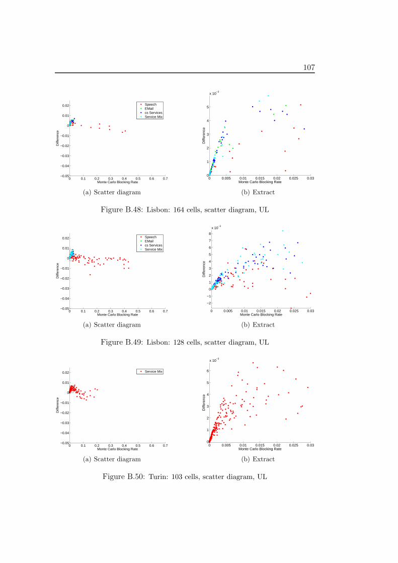
107
0 0.1 0.2 0.3 0.4 0.5 0.6 0.7−0.05
−0.04
−0.03
−0.02
−0.01
0
0.01
0.02
Monte Carlo Blocking Rate
Diff
eren
ce
SpeechEMailcs ServicesService Mix
(a) Scatter diagram
0 0.005 0.01 0.015 0.02 0.025 0.030
1
2
3
4
5
x 10−3
Monte Carlo Blocking Rate
Diff
eren
ce
(b) Extract
Figure B.48: Lisbon: 164 cells, scatter diagram, UL
0 0.1 0.2 0.3 0.4 0.5 0.6 0.7−0.05
−0.04
−0.03
−0.02
−0.01
0
0.01
0.02
Monte Carlo Blocking Rate
Diff
eren
ce
SpeechEMailcs ServicesService Mix
(a) Scatter diagram
0 0.005 0.01 0.015 0.02 0.025 0.03
−2
−1
0
1
2
3
4
5
6
7
8
x 10−3
Monte Carlo Blocking Rate
Diff
eren
ce
(b) Extract
Figure B.49: Lisbon: 128 cells, scatter diagram, UL
0 0.1 0.2 0.3 0.4 0.5 0.6 0.7−0.05
−0.04
−0.03
−0.02
−0.01
0
0.01
0.02
Monte Carlo Blocking Rate
Diff
eren
ce
Service Mix
(a) Scatter diagram
0 0.005 0.01 0.015 0.02 0.025 0.030
1
2
3
4
5
6
x 10−3
Monte Carlo Blocking Rate
Diff
eren
ce
(b) Extract
Figure B.50: Turin: 103 cells, scatter diagram, UL
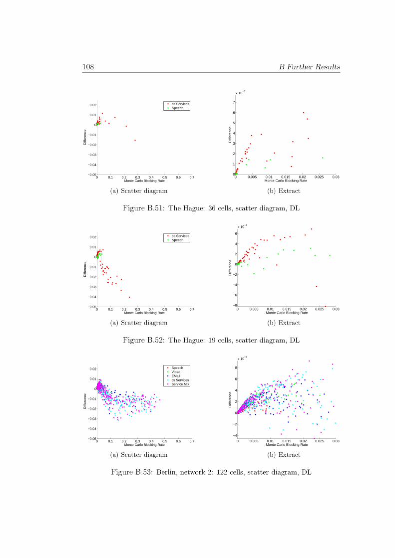
108 B Further Results
0 0.1 0.2 0.3 0.4 0.5 0.6 0.7−0.05
−0.04
−0.03
−0.02
−0.01
0
0.01
0.02
Monte Carlo Blocking Rate
Diff
eren
ce
cs ServicesSpeech
(a) Scatter diagram
0 0.005 0.01 0.015 0.02 0.025 0.030
1
2
3
4
5
6
7
x 10−3
Monte Carlo Blocking Rate
Diff
eren
ce
(b) Extract
Figure B.51: The Hague: 36 cells, scatter diagram, DL
0 0.1 0.2 0.3 0.4 0.5 0.6 0.7−0.05
−0.04
−0.03
−0.02
−0.01
0
0.01
0.02
Monte Carlo Blocking Rate
Diff
eren
ce
cs ServicesSpeech
(a) Scatter diagram
0 0.005 0.01 0.015 0.02 0.025 0.03−8
−6
−4
−2
0
2
4
6
x 10−3
Monte Carlo Blocking Rate
Diff
eren
ce
(b) Extract
Figure B.52: The Hague: 19 cells, scatter diagram, DL
0 0.1 0.2 0.3 0.4 0.5 0.6 0.7−0.05
−0.04
−0.03
−0.02
−0.01
0
0.01
0.02
Monte Carlo Blocking Rate
Diff
eren
ce
SpeechVideoEMailcs ServicesService Mix
(a) Scatter diagram
0 0.005 0.01 0.015 0.02 0.025 0.03
−4
−2
0
2
4
6
8
x 10−3
Monte Carlo Blocking Rate
Diff
eren
ce
(b) Extract
Figure B.53: Berlin, network 2: 122 cells, scatter diagram, DL

109
0 0.1 0.2 0.3 0.4 0.5 0.6 0.7−0.05
−0.04
−0.03
−0.02
−0.01
0
0.01
0.02
Monte Carlo Blocking Rate
Diff
eren
ce
SpeechEMailcs ServicesService Mix
(a) Scatter diagram
0 0.005 0.01 0.015 0.02 0.025 0.03
−4
−2
0
2
4
6
8
x 10−3
Monte Carlo Blocking Rate
Diff
eren
ce
(b) Extract
Figure B.54: Lisbon: 164 cells, scatter diagram, DL
0 0.1 0.2 0.3 0.4 0.5 0.6 0.7−0.05
−0.04
−0.03
−0.02
−0.01
0
0.01
0.02
Monte Carlo Blocking Rate
Diff
eren
ce
SpeechEMailcs ServicesService Mix
(a) Scatter diagram
0 0.005 0.01 0.015 0.02 0.025 0.03−6
−4
−2
0
2
4
6
8
10
12x 10
−3
Monte Carlo Blocking Rate
Diff
eren
ce
(b) Extract
Figure B.55: Lisbon: 128 cells, scatter diagram, DL
0 0.1 0.2 0.3 0.4 0.5 0.6 0.7−0.05
−0.04
−0.03
−0.02
−0.01
0
0.01
0.02
Monte Carlo Blocking Rate
Diff
eren
ce
Service Mix
(a) Scatter diagram
0 0.005 0.01 0.015 0.02 0.025 0.030
0.5
1
1.5
2
2.5
3
x 10−3
Monte Carlo Blocking Rate
Diff
eren
ce
(b) Extract
Figure B.56: Turin: 103 cells, scatter diagram, DL

110 B Further Results

C Zusammenfassung
Das Ziel der vorliegenden Arbeit ist es, ein mathematisches Modell zu ent-wickeln, das die Blockier Raten der Zellen in einem UMTS Funknetz effizientapproximiert. Die Blockier Rate bezeichnet den Anteil an Teilnehmern, deraufgrund der beschrankten Funkressourcen einer Antenne nicht bedient wer-den kann. Sie stellt ein wichtiges Kriterium fur die Qualitatsbewertung einesFunknetzdesigns dar. Jedoch ist bisher kein Modell bekannt, das die durch-schnittliche Blockier Rate schnell und verlasslich vorhersagen kann. DieSchwierigkeit dabei besteht darin, dass die Kapazitat einer UMTS Funkzelleschwankt.
In dieser Arbeit werden zwei Ansatze vorgestellt, um die Blockier Ratenin UMTS Funknetzen zu approximieren. Diese Methoden basieren auf einembereits vorhandenen Modell. In der ersten Methode werden dessen Un-genauigkeiten reduziert, indem der Erwartungswert der durchschnittlichenBlockier Rate in Abhangigkeit von der Interferenz aus der eigenen Zelleberechnet wird. In der zweiten Methode wird das vorliegende Problem alseine Art gebrochenes Rucksack Problem aufgefasst. Wir betrachten dabeidie Verteilung des Gesamtgewichts aller Nutzer in einer Funkzelle. Abhangigvon diesem akkumulierten Gewicht bestimmen wir den Erwartungswert derdurchschnittlichen Blockier Rate. In beiden Ansatzen wird die Interferenzaus anderen Funkzellen durch Durchschnittswerte abgeschatzt. Diese Schat-zungen werden mit zusatzlichem Aufwand prazisiert. Außerdem leiten wiranalytisch her, dass die Ergebnisse beider Modelle gleich sind.
Umfangreiche Tests belegen, dass wir mit den entwickelten Methodeneinen sehr guten Kompromiss zwischen Genauigkeit und Komplexitat gefun-den haben. Die Eigenschaften des Basismodells sind in Grundzugen nochvorhanden. D. h., in niedrigen Bereichen wird die Blockier Rate etwas un-terschatzt und in hoheren leicht uberschatzt. Doch im Gegensatz zu vorherliegen diese systematischen Schatzfehler in einem durchaus akzeptablen Be-reich. Die Komplexitat der beiden vorgestellten Ansatze ist gleich. ImGegensatz zu existierenden Methoden mit vergleichbarer Genauigkeit sinddie durchschnittlichen Laufzeiten extrem kurz.
111

112 C Zusammenfassung

List of Figures
2.1 Block diagram of a communications system . . . . . . . . . . . 62.2 Cells in a UMTS radio network . . . . . . . . . . . . . . . . . . 72.3 Operating mode of Code Division Multiplex . . . . . . . . . . . . 92.4 Wideband spreading . . . . . . . . . . . . . . . . . . . . . . . 102.5 Interference attenuation in CDMA . . . . . . . . . . . . . . . 112.6 Average traffic distribution for one service . . . . . . . . . . . . . 17
3.1 Power and blocking rate in downlink for an isolated cell . . . . . . 29
4.1 Distribution of the random variable for service speech telephony . 544.2 Distribution of the random variable for a service mix . . . . . . . 54
7.1 Synth.: one cell, speech telephony . . . . . . . . . . . . . . . . . 727.2 Synth.: one cell, cs services . . . . . . . . . . . . . . . . . . . . . 727.3 Synth.: one cell, service mix . . . . . . . . . . . . . . . . . . . . 727.4 Synth.: two cells, speech telephony, uplink . . . . . . . . . . . . . 747.5 Synth.: two cells, speech telephony, downlink . . . . . . . . . . . 747.6 Synth.: two cells, cs services, uplink . . . . . . . . . . . . . . . . 747.7 Synth.: two cells, cs services, downlink . . . . . . . . . . . . . . . 757.8 Synth.: two cells, service mix, uplink . . . . . . . . . . . . . . . . 757.9 Synth.: two cells, service mix, downlink . . . . . . . . . . . . . . 757.10 Examples for speech telephony, uplink . . . . . . . . . . . . . . . 777.11 Berlin, network 2: 122 cells, uplink . . . . . . . . . . . . . . . . . 777.12 Berlin: 122 cells, different service mixes, downlink . . . . . . . . . 787.13 Berlin, network 1: 122 cells, scatter diagram, uplink . . . . . . . . 797.14 Berlin, network 1: 122 cells, scatter diagram, downlink . . . . . . 797.15 Examples for overestimation, downlink . . . . . . . . . . . . . . . 80
B.1 Legend for all following figures . . . . . . . . . . . . . . . . . . . 91B.2 The Hague: 36 cells, speech telephony, UL . . . . . . . . . . . . . 91B.3 The Hague: 36 cells, speech telephony, DL . . . . . . . . . . . . . 92B.4 The Hague: 36 cells, cs services . . . . . . . . . . . . . . . . . . 92
113

114 List of Figures
B.5 The Hague: 19 cells, speech telephony, UL . . . . . . . . . . . . . 92B.6 The Hague: 19 cells, speech telephony, traffic scaling 5.8, DL . . . 93B.7 The Hague: 19 cells, cs services, UL . . . . . . . . . . . . . . . . 93B.8 The Hague: 19 cells, cs services, DL . . . . . . . . . . . . . . . . 93B.9 Berlin, network 1: 122 cells, speech telephony, UL . . . . . . . . . 94B.10 Berlin, network 1: 122 cells speech telephony, DL . . . . . . . . . 94B.11 Berlin, network 1: 122 cells, video telephony, UL . . . . . . . . . 94B.12 Berlin, network 1: 122 cells, video telephony, DL . . . . . . . . . 95B.13 Berlin, network 1: 122 cells, e-mail, UL . . . . . . . . . . . . . . 95B.14 Berlin, network 1: 122 cells, e-mail, DL . . . . . . . . . . . . . . 95B.15 Berlin, network 1: 122 cells, cs services, UL . . . . . . . . . . . . 96B.16 Berlin, network 1: 122 cells, cs services, 0.56, DL . . . . . . . . . 96B.17 Berlin, network 1: 122 cells, service mix, UL . . . . . . . . . . . . 96B.18 Berlin, network 1: 122 cells, service mix, DL . . . . . . . . . . . . 97B.19 Berlin, network 2: 122 cells, speech telephony, 1.8, UL . . . . . . . 97B.20 Berlin, network 2: 122 cells, speech telephony, DL . . . . . . . . . 97B.21 Berlin, network 2: 122 cells, video telephony, 2.4, UL . . . . . . . 98B.22 Berlin, network 2: 122 cells, video telephony, DL . . . . . . . . . 98B.23 Berlin, network 2: 122 cells, e-mail, 1000, UL . . . . . . . . . . . 98B.24 Berlin, network 2: 122 cells, e-mail, DL . . . . . . . . . . . . . . 99B.25 Berlin, network 2: 122 cells, cs services, UL . . . . . . . . . . . . 99B.26 Berlin, network 2: 122 cells, cs services, DL . . . . . . . . . . . . 99B.27 Berlin, network 2: 122 cells, service mix, UL . . . . . . . . . . . . 100B.28 Berlin, network 2: 122 cells, service mix, 0.48, DL . . . . . . . . . 100B.29 Lisbon: 164 cells, speech telephony . . . . . . . . . . . . . . . . . 100B.30 Lisbon: 164 cells, e-mail, UL . . . . . . . . . . . . . . . . . . . . 101B.31 Lisbon: 164 cells, e-mail, DL . . . . . . . . . . . . . . . . . . . . 101B.32 Lisbon: 164 cells, cs services, UL . . . . . . . . . . . . . . . . . . 101B.33 Lisbon: 164 cells, cs services, DL . . . . . . . . . . . . . . . . . . 102B.34 Lisbon: 164 cells, service mix, UL . . . . . . . . . . . . . . . . . 102B.35 Lisbon: 164 cells, service mix, DL . . . . . . . . . . . . . . . . . 102B.36 Lisbon: 128 cells, speech telephony, 1.6, UL . . . . . . . . . . . . 103B.37 Lisbon: 128 cells, speech telephony, DL . . . . . . . . . . . . . . 103B.38 Lisbon: 128 cells, e-mail, DL . . . . . . . . . . . . . . . . . . . . 103B.39 Lisbon: 128 cells, cs services, UL . . . . . . . . . . . . . . . . . . 104B.40 Lisbon: 128 cells, cs services, DL . . . . . . . . . . . . . . . . . . 104B.41 Lisbon: 128 cells, service mix, UL . . . . . . . . . . . . . . . . . 104B.42 Lisbon: 128 cells, service mix, DL . . . . . . . . . . . . . . . . . 105B.43 Turin: 103 cells, service mix, UL . . . . . . . . . . . . . . . . . . 105B.44 Turin: 103 cells, service mix, DL . . . . . . . . . . . . . . . . . . 105B.45 The Hague: 36 cells, scatter diagram, UL . . . . . . . . . . . . . 106

List of Figures 115
B.46 The Hague: 19 cells, scatter diagram, UL . . . . . . . . . . . . . 106B.47 Berlin, network 2: 122 cells, scatter diagram, UL . . . . . . . . . 106B.48 Lisbon: 164 cells, scatter diagram, UL . . . . . . . . . . . . . . . 107B.49 Lisbon: 128 cells, scatter diagram, UL . . . . . . . . . . . . . . . 107B.50 Turin: 103 cells, scatter diagram, UL . . . . . . . . . . . . . . . 107B.51 The Hague: 36 cells, scatter diagram, DL . . . . . . . . . . . . . 108B.52 The Hague: 19 cells, scatter diagram, DL . . . . . . . . . . . . . 108B.53 Berlin, network 2: 122 cells, scatter diagram, DL . . . . . . . . . 108B.54 Lisbon: 164 cells, scatter diagram, DL . . . . . . . . . . . . . . . 109B.55 Lisbon: 128 cells, scatter diagram, DL . . . . . . . . . . . . . . . 109B.56 Turin: 103 cells, scatter diagram, DL . . . . . . . . . . . . . . . 109

116 List of Figures

Bibliography
[1] C. Balzanelli, A. Munna, and R. Verdone. WCDMA downlink capacity:part 1. In Proc. of IEEE PIMRC’2003, Beijing, China, Sept. 2003.
[2] T. Benkner and C. Stepping. UMTS: Universal Mobile Telecommunica-tions System. J. Schlembach Fachverlag, Weil der Stadt, 2002.
[3] J. Davidson. Stochastic Limit Theory. Oxford University Press, 1994.
[4] B. De Schutter and B. De Moor. The extended linear complementarityproblem. Math. Programming, 71(3):289–325, Dec. 1995.
[5] M. Duque-Anton. Mobilfunknetze: Grundlagen, Dienste und Protokolle.Vieweg Verlag, Braunschweig/Wiesbaden, 1st edition, May 2002.
[6] A. Eisenblatter, H.-F. Geerdes, T. Koch, A. Martin, and R. Wessaly.UMTS radio network evaluation and optimization beyond snapshots.Math. Meth. Oper. Res., 63(1), 2006.
[7] A. Eisenblatter, H.-F. Geerdes, and N. Rochau. Analytical approximateload control in W-CDMA radio networks. In Proceedings of VTC-2005Fall, Dallas, TX, Sept. 2005. IEEE.
[8] A. Eisenblatter, H.-F. Geerdes, and U. Turke. Public UMTS radio net-work evaluation and planning scenarios. Internat. J. on Mobile NetworkDesign and Innovation, 2005.
[9] J. Elstrodt. Maß- und Integrationstheorie. Springer-Verlag, 2nd edition,1999.
[10] G. S. Fishman. Monte Carlo: Concepts, Algorithms and Applications.Springer Series in Operations Research. Springer Verlag, New York,USA, 1996.
[11] H.-O. Georgii. Stochastik: Einfuhrung in die Wahrscheinlichkeitstheorieund Statistik. de Gruyter, Berlin, Germany, 2nd edition, 2004.
117

118 Bibliography
[12] S. Haykin and M. Moher. Modern Wireless Communications. PearsonEducation, Inc., 2005.
[13] H. Holma and A. Toskala, editors. WCDMA for UMTS. John Wiley &Sons, Ltd., revised edition, 2001.
[14] K.-D. Kammeyer. Nachrichtenubertragung. B.G. Teubner Verlag, 3rdedition, 2004.
[15] U. Krengel. Einfuhrung in die Wahrscheinlichkeitstheorie und Statis-tik. vieweg studium – Aufbaukurs Mathematik. Vieweg Verlag, Braun-schweig/Wiesbaden, 6th edition, Feb. 2002.
[16] J. Laiho, A. Wacker, and T. Novosad, editors. Radio Network Planningand Optimisation for UMTS. John Wiley & Sons, Ltd, 2002.
[17] N. Madras. Lectures on Monte Carlo Methods. American MathematicalSociety, Providence, Rhode Island, 2002.
[18] Momentum Project, IST-2000-28088. Momentum pub-lic UMTS planning scenarios. Avaliable online athttp://momentum.zib.de/data.php, 2003.
[19] Cost 273: Mobile Radio Access Network Reference Scenarios(morans). http://www.cost273.org/morans/, 2004.
[20] P. E. Pfeiffer and D. A. Schum. Introduction to Applied Probability.Academic Press, New York, 1973.
[21] U. Turke, T. Winter, R. Perera, E. Lamers, E. Meijerink, E. R. Fled-derus, and A. Serrador. Comparison of different simulation approachesfor cell performance evaluation. Technical Report D2.2, IST-2000-28088Momentum, 2002.
[22] B. Walke. Mobilfunknetze und ihre Protokolle, volume 1. B. G. TeubnerVerlag, Stuttgart, 1998.
[23] B. Walke, M. P. Althoff, and P. Seidenberg. UMTS–Ein Kurs. J. Schlem-bach Fachverlag, Weil der Stadt, 2nd edition, 2002.
[24] Wikipedia. Universal Mobile Telecommunications System – Wikipedia,Die freie Enzyklopadie. http://de.wikipedia.org/wiki/UMTS, 2005.[Online; accessed 09.11.2005].