Approximate Frequency Counts over Data Streams

Gurmeet Singh Manku (Standford) Rajeev Motwani

(Standford)Presented by Michal Spivak

November, 2003

The Problem…

Stream

Identify all elements whose current frequency exceeds support threshold s = 0.1%.

Related problem…

Stream

Identify all subsets of items whose current frequency exceeds s=0.1%

Purpose of this paperPresent an algorithm for computing frequency counts exceeding a user-specified threshold over data streams with the following advantages:

Simple Low memory footprint Output is approximate but guaranteed not to

exceed a user specified error parameter. Can be deployed for streams of singleton items

and handle streams of variable sized sets of items.

Overview

Introduction Frequency counting applications Problem definition Algorithm for Frequent Items Algorithm for Frequent Sets of Items Experimental results Summary

Introduction

Motivating examples Iceberg Query

Perform an aggregate function over an attribute and eliminate those below some threshold.

Association RulesRequire computation of frequent itemsets.

Iceberg DatacubesGroup by’s of a CUBE operator whose aggregate frequency exceeds threshold

Traffic measurement Require identification of flows that exceed a certain fraction of total traffic

What’s out there today… Algorithms that compute exact results Attempt to minimize number of data

passes (best algorithms take two passes).

Problems when adapted to streams: Only one pass is allowed. Results are expected to be available with

short response time. Fail to provide any a-priori guarantee on

the quality of their output.

Why Streams?Streams vs. Stored data

Volume of a stream over its lifetime can be huge

Queries for streams require timely answers, response times need to be small

As a result it is not possible to store the stream as an entirety.

Frequency counting applications

Existing applications for the following problems Iceberg Query

Perform an aggregate function over an attribute and eliminate those below some threshold.

Association RulesRequire computation of frequent itemsets.

Iceberg DatacubesGroup by’s of a CUBE operator whose aggregate frequency exceeds threshold

Traffic measurement Require identification of flows that exceed a certain fraction of total traffic

Iceberg QueriesIdentify aggregates that exceed a user-specified threshold r

One of the published algorithms to compute iceberg queries efficiently uses repeated hashing over multiple passes.*

Basic Idea: In the first pass a set of counters is maintained Each incoming item is hashed to one of the counters

which is incremented These counters are then compressed to a bitmap, with a 1

denoting large counter value In the second pass exact frequencies are maintained for

only those elements that hash to a counter whose bitmap value is 1

This algorithm is difficult to adapt for streams because it requires two passes

* M. FANG, N. SHIVAKUMAR, H. GARCIA-MOLINA,R. MOTWANI, AND J. ULLMAN. Computing icebergqueries efficiently. In Proc. of 24th Intl. Conf. on Very Large Data Bases, pages 299–310, 1998.

Association RulesDefinitions Transaction – subset of items drawn from I, the

universe of all Items. Itemset X I has support s if X occurs as a

subset at least a fraction - s of all transactions Associations rules over a set of transactions

are of the form X=>Y, where X and Y are subsets of I such that X∩Y = 0 and XUY has support exceeding a user specified threshold s.

Confidence of a rule X => Y is the value support(XUY) / support(X)

U|

Example - Market basket analysis

Transaction Id Purchased Items 1 {1, 2, 3}2 {1, 4}3 {1, 3}4 {2, 5, 6}

For support = 50%, confidence = 50%, we have the following rules1 => 3 with 50% support and 66% confidence3 => 1 with 50% support and 100% confidence

Reduce to computing frequent itemsets

TID Items1 {1, 2, 3}2 {1, 3}3 {1, 4}4 {2, 5, 6}

Frequent Itemset Support{1} 75%{2} 50%{3} 50%{1, 3} 50%

For the rule 1 => 3:•Support = Support({1, 3}) = 50%•Confidence = Support({1,3})/Support({1}) = 66%

For support = 50%, confidence = 50%

Toivonen’s algorithm

Based on sampling of the data stream. Basically, in the first pass, frequencies are

computed for samples of the stream, and in the second pass these the validity of these items is determined.

Can be adapted for data stream Problems:

- false negatives occur because the error in frequency counts is two sided- for small values of , the number of samples is enormous ~ 1/ (100 million samples)

Network flow identification Flow – sequence of transport layer packets that

share the same source+destination addresses Estan and Verghese proposed an algorithm for

this identifying flows that exceed a certain threshold.The algorithm is a combination of repeated hashing and sampling, similar to those for iceberg queries.

Algorithm presented in this paper is directly applicable to the problem of network flow identification. It beats the algorithm in terms of space and requirements.

Problem definition

Problem Definition Algorithm accepts two user-specified

parameters- support threshold s E (0,1)- error parameter ε E (0,1)- ε << s

N – length of stream (i.e no. of tuples seen so far)

Itemset – set of items Denote item(set) to be item or itemset At any point of time, the algorithm can be asked

to produce a list of item(set)s along with their estimated frequency.

Approximation guarantees

All item(set)s whose true frequency exceeds sN are output. There are no false negatives.

No item(set)s whose true frequency is less than (s- ε(N is output.

Estimated frequencies are less than true frequencies by at most εN

Input Example S = 0.1% ε as a rule of thumb, should be set to one-tenth or one-

twentieth of s. ε = 0.01%

As per property 1, ALL elements with frequency exceeding 0.1% will be output.

As per property 2, NO element with frequency below 0.09% will be output

Elements between 0.09% and 0.1% may or may not be output. Those that “make their way” are false positives

As per property 3, all individual frequencies are less than their true frequencies by at most 0.01%

Problem Definition cont…

An algorithm maintains an ε-deficient synopsis if its output satisifies the aforementioned properties

Goal: to devise algorithms to support ε-deficient synopsis using as little main memory as possible

The Algorithms for frequent Items

Sticky Sampling Lossy Counting

Sticky Sampling Algorithm

Stream

Create counters by sampling

341530

283141233519

Notations…

Data structure S - set of entries of the form (e,f)

f – estimates the frequency of an element e.

r – sampling rate. Sampling an element with rate = r means we select the element with probablity = 1/r

Sticky Sampling cont… Initially – S is empty, r = 1. For each incoming element e

if (e exists in S) increment corresponding f

else {sample element with rate r

if (sampled)add entry (e,1) to S

elseignore

}

The sampling rate

Let t = 1/ ε log(s-1 -1) ( = probability of failure)

First 2t elements are sampled at rate=1

The next 2t elements at rate=2 The next 4t elements at rate=4 and so on…

Sticky Sampling cont…

Whenever the sampling rate r changes: for each entry (e,f) in S repeat {

toss an unbiased coinif (toss is not successful)

diminsh f by oneif (f == 0) {

delete entry from Sbreak

}} until toss is successful

Sticky Sampling cont…

The number of unsuccessful coin tosses folows a geometric distribution.

Effectively, after each rate change S is transformed to exactly the state it would have been in, if the new rate had been used from the beginning.

When a user requests a list of items with threshold s, the output are those entries in S where f ≥ (s – ε)N

Theorem 1

Sticky Sampling computes an ε-deficient synopsis with probability at least 1 - using at most 2/ ε log(s-1 -1) expected number of entries.

Theorem 1 - proof First 2t elements find their way into S When r ≥ 2

N = rt + rt` ( t`E [1,t) ) => 1/r ≥ t/N Error in frequency corresponds to a sequence

of unsuccessful coin tosses during the first few occurrences of e.the probability that this length exceeds εN is at most (1 – 1/r)εN < (1 – t/N)-εN < e-εt

Number of elements with f > s is no more than 1/s => the probability that the estimate for any of them is deficient by εN is at most e-εt/s

Theorem 1 – proof cont…

Probability of failure should be at most . This yieldse-εt/s <

t ≥ 1/ ε log(s-1 -1)

since the space requirements are 2t, the space bound follows…

Sticky Sampling summary The algorithm name is called sticky sampling

because S sweeps over the stream like a magnet, attracting all elements which already have an entry in S

The space complexity is independent of N The idea of maintaining samples was first

presented by Gibbons and Matias who used it to solve the top-k problem.

This algorithm is different in that the sampling rate r increases logarithmically to produce ALL items with frequency > s, not just the top k

Lossy Counting

bucket 1 bucket 2 bucket 3

Divide the stream into bucketsKeep exact counters for items in the bucketsPrune entrys at bucket boundaries

Lossy Counting cont…

A deterministic algorithm that computes frequency counts over a stream of singleitem transactions, satisfying the guarantees outlined in Section 3 using at most 1/εlog(εN) space where N denotes the current length of the stream.

The user specifies two parameters:- support s- error ε

Definitions The incoming stream is conceptually

divided into buckets of width = ceil(1/ Buckets are labeled with bucket ids,

starting from 1 Denote the current bucket id by bcurrent

whose value is ceil(N/ Denote fe to be the true frequency of an

element e in the stream seen so far Data stucture D is a set of entries of the

form (e,f,)

The algorithm Initially D is empty Receive element e

if (e exists in D)increment its frequency (f) by 1

elsecreate a new entry (e, 1, bcurrent – 1)

If it bucket boundary prune D by the following the rule:(e,f,) is deleted if f + ≤ bcurrent

When the user requests a list of items with threshold s, output those entries in D where f ≥ (s – ε)N

Some algorithm facts For an entry (e,f,) f represents the

exact frequency count for e ever since it was inserted into D.

The value is the maximum number of times e could have occurred in the first bcurrent – 1 buckets ( this value is exactly bcurrent – 1)

Once a value is inserted into D its value is unchanged

Lossy counting in action

D is Empty

FrequencyCounts

At window boundary, remove entries that for them f+≤ bcurrent

+

First Bucket

Lossy counting in action cont

FrequencyCounts

Next Bucket

+

At window boundary, remove entries that for them f+≤ bcurrent

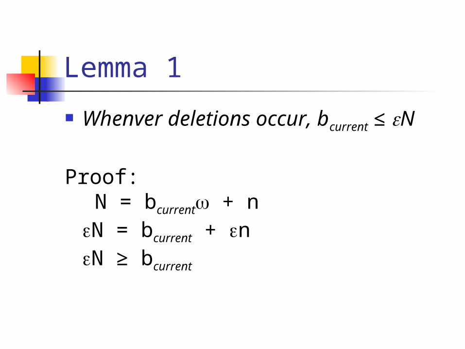
Lemma 1

Whenver deletions occur, bcurrent ≤ N

Proof: N = bcurrent + nN = bcurrent + nN ≥ bcurrent

Lemma 2 Whenever an entry (e,f,) gets deleted

fe ≤ bcurrent

Proof by induction Base case: bcurrent = 1

(e,f,) is deleted only if f = 1 Thus fe ≤ bcurrent (fe = f) Induction step:

- Consider (e,f,) that gets deleted for some bcurrent > 1. - This entry was inserted when bucket +1 was being processed. - It was deleted at late as the time as bucket became full. - By induction the true frequency for e was no more than . - f is the true frequency of e since it was inserted.- fe ≤ f+ combined with the deletion rule f+≤ bcurrent =>

fe ≤ bcurrent

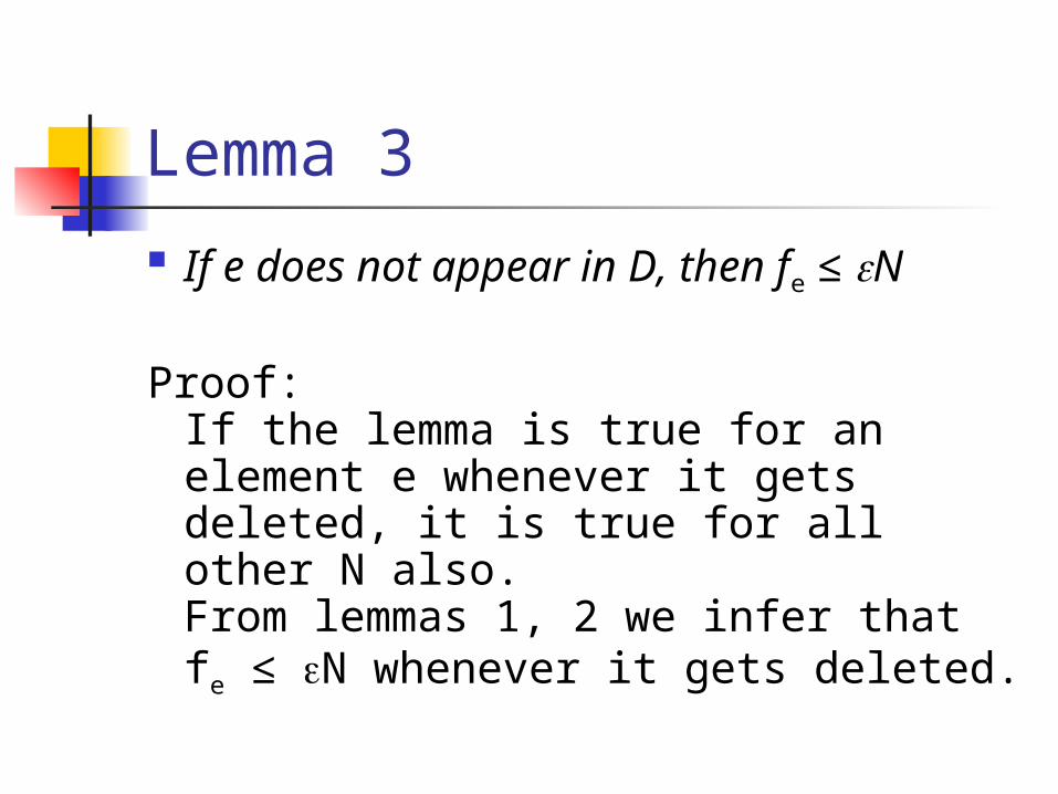
Lemma 3

If e does not appear in D, then fe ≤ N

Proof: If the lemma is true for an element e whenever it gets deleted, it is true for all other N also.From lemmas 1, 2 we infer that fe ≤ N whenever it gets deleted.

Lemma 4 If (e,f,) D, then f ≤ fe ≤ f + N

Proof:If =0, f=fe.Otherwise

e was possibly deleted in the first buckets.From lemma 2 fe ≤ f+≤ bcurrent – 1 ≤ N

Conclusion f ≤ fe ≤ f + N

Lossy Counting cont…

Lemma 3 shows that all elements whose true frequency exceed N have entries in D

Lemma 4 shows that the estimated frequency of all such elements are accurate to within N

=> D correctly maintains an -deficient synopsis

Theorem 2

Lossy counting computes an e-deficient synopsis using at most 1/log(N) entries

Theorem 2 - proof Let B = bcurrent

di – denote the number of entries in D whose bucket id is B - i + 1 (iE[1,B])

e corresponding to di must occur at least i times in buckets B-i+1 through B, otherwise it would have been deleted

We get the following constraint:(1) idi ≤ jfor j = 1,2,…B. i = 1..j

Theorem 2 – proof

The following inequality can be proved by induction:di ≤ i for j = 1,2,…B i = 1..j

|D| = di for i = 1..B From the above inequality

|D| ≤ i ≤ 1/logB = 1/log(N)

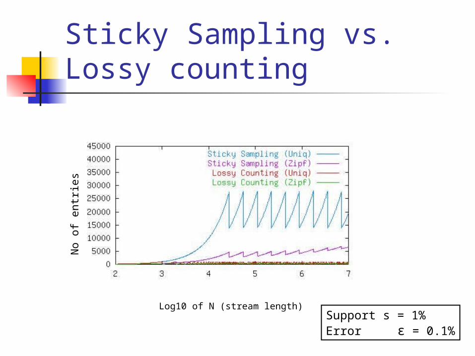
Sticky Sampling vs. Lossy counting

Support s = 1%Error ε = 0.1%

No o

f entr

ies

Log10 of N (stream length)

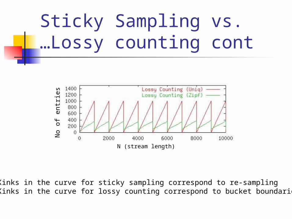
Sticky Sampling vs.Lossy counting cont…

N (stream length)

No o

f entr

ies

Kinks in the curve for sticky sampling correspond to re-samplingKinks in the curve for lossy counting correspond to bucket boundaries

Sticky Sampling vs. Lossy counting cont…

SS – Sticky Sampling LC – Lossy CountingZipf – zipfian distribution Uniq – stream with no duplicates

sSS

worstLC

worstSS

ZipfLC

ZipfSS

UniqLC

Uniq

0.1%1.0%27K9K6K41927K1K

0.05%0.5%58K17K11K70958K2K

0.01%0.1%322K69K37K2K322K10K

0.005%0.05%672K124K62K4K672K20K

Sticky Sampling vs. Lossy summary

Lossy counting is superior by a large factor

Sticky sampling performs worse because of its tendency to remember every unique element that gets sampled

Lossy counting is good at pruning low frequency elements quickly

Comparison with alternative approaches

Toivonen – sampling algorithm for association rules.

Sticky sampling beats the approach by roughly a factor of

Comparison with alternative approaches

cont… KPS02 – In the first path the algorithm

maintains 1/ elements with their frequencies. If a counter exists for an element it is increased, if there is a free counter it is inserted, otherwise all existing counters are reduced by one

Can be used to maintain -deficient synopsis with exactly 1/ space

If the input stream is ZipfianLossy Counting takes less than 1/ spacefor =0.01% roughly 2000 entries ~ 20% 1/

Frequent Sets of Items

From theory to Practice

Frequent Sets of Items

Stream

Identify all subsets of items whose current frequency exceeds s = 0.1%.

Frequent itemsets algorithm Input: stream of transactions, each

transaction is a set of items from I N: length of the stream User specifies two parameters:

support s, error Challenge:

- handling variable sized transactions- avoiding explicit enumeration of all subsets of any transaction

Notations Data structure D – set of entries of the form

(set, f, ) Transactions are divided into buckets = ceil(1/) – no. of transactions in each bucket bcurrent – current bucket id Transactions are not processed one by one.

Main memory is filled with as many transactions as possible. Processing is done on a batch of transactions. – no. of buckets in main memory in the current batch being processed.

Update D UPDATE_SET: for each entry (f,set,) E

D, update f by counting occurrences of set in the current batch. If the updated entry satisfies f+≤ bcurrent, we delete this entry

NEW_SET: if a set set has frequency f ≥ in the current batch and set does not occur in D, create a new entry (set,f,bcurrent – )

Algorithm facts If fset ≥ N it has an entry in D If (set,f,)ED then the true frequency of

fset satisfies the inequality f≤ fset ≤ f+ When a user requests a list of items with

threshold s, output those entries in D wheref ≥ (s-)N

B needs to be a large number. Any subset of I that occurs B+1 times or more contributes to D.

Three modules

BUFFER

TRIE

SUBSET-GEN

maintains the data structure D

operates on the current batch of transactions

repeatedly reads in a batch of transactionsinto available main memory

implement UPDATE_SET, NEW_SET

Module 1 - Buffer

bucket 1 bucket 2 bucket 3 bucket 4 bucket 5 bucket 6

In Main Memory

Read a batch of transactions Transactions are laid out one after the other in a big array A bitmap is used to remember transaction boundaries After reading in a batch, BUFFER sorts each transaction by its item-id’s

Module 2 - TRIE

50

40

30

31 29 32

45

42

50 40 30 31 29 45 32 42 Sets with frequency counts

Module 2 – TRIE cont… Nodes are labeled {item-id, f, , level} Children of any node are ordered by their item-

id’s Root nodes are also ordered by their item-id’s A node represents an itemset consisting of item-

id’s in that node and all its ancestors TRIE is maintained as an array of entries of the

form {item-id, f, , level} (pre-order of the trees). Equivalent to a lexicographic ordering of subsets it encodes.

No pointers, level’s compactly encode the underlying tree structure.

Module 3 - SetGen

BUFFER

3 3 3 4 2 2 1 2 1 3 1 1

Frequency countsof subsetsin lexicographic order

SetGen uses the following pruning rule:if a subset S does not make its way into TRIE after application of both UPDATE_SET and NEW_SET, then no supersets of S should be considered

Overall Algorithm

BUFFER

3 3 3 4 2 2 1 2 1 3 1 1 SUBSET-GEN

TRIE new TRIE

Efficient ImplementationsBuffer

If item-id’s are successive integers from 1 thru |I|, and I is small enough (less than 1 million) Maintain exact frequency counts for singleton sets. Prune away those item-id’s whose frequency is less than N and then sort the transactions

If |I| = 105, array size = 0.4 MB

Efficient ImplementationsTRIE Take advantage of the fact that the sets

produced by SetGen are lexicographic. Maintain TRIE as a set of fairly large-

sized chunks of memory instead of one huge array

Instead of modifying the original TRIE, create a new TRIE.

Chunks from the old TRIE are freed as soon as they are not required.

By the time SetGen finishes, the chunks of the original TRIE have been discarder.

Efficient ImplementationsSetGen

Employs a priority queue called Heap Initially contains pointers to smallest

item-id’s of all transactions in buffer Duplicate members are maintained

together and constitute a single item in the Heap. Chain all these pointers together.

Derive the space from BUFFER. Change item-id’s with pointers.

Efficient ImplementationsSetGen cont…

123145245613

12

Efficient ImplementationsSetGen cont…

Repeatedly process the smallest item-id in Heap to generate singleton sets.

If the singleton belongs to TRIE after UPDATE_SET and NEW_SET try to generate the next set by extending the current singleton set.

This is done by invoking SetGen recursively with a new Heap created out of successors of the pointers to item-id’s just processed and removed.

When the recursive call returns, the smallest entry in Heap is removed and all successors of the currently smallest item-id are added.

Efficient ImplementationsSetGen cont…

123125245613

12

2

3

System issues and optimizations Buffer scans the incoming stream by

memory mapping the input file. Use standard qsort to sort transactions Threading SetGen and Buffer does not

help because SetGen is significantly slower.

The rate at which tries are scanned is much smaller than the rate at which sequiential disk I/O can be done

Possible to maintain TRIE on disk without loss in performance

System issues and optimizationsTRIE on disk advantages

The size of TRIE is not limited by main memory – this algorithm can function with a low amount of main memory.

Since most available main memory can be devoted to BUFFER, this algorithm can handle smaller values of than other algorithms can handle.

Novel features of this technique

No candidate generation phase. Compact disk-based tries is novel Able to compute frequent itemsets

under low memory conditions. Able to handle smaller values of

support threshold than previously possible.

Experimental results

Experimental Results

IBM synthetic dataset T10.I4.1000K N = 1Million Avg Tran Size = 10 Input Size = 49MB

IBM synthetic dataset T15.I6.1000K N = 1Million Avg Tran Size = 15 Input Size = 69MB

Frequent word pairs in 100K web documents N = 100K Avg Tran Size = 134 Input Size = 54MB

Frequent word pairs in 806K Reuters newsreports N = 806K Avg Tran Size = 61 Input Size = 210MB

What is studied

Support threshold s Number of transactions N Size of BUFFER B Total time taken t

set = 0.1s

Varying buffer sizes and support s

Tim

e t

ake

n in s

eco

nds

Support threshold s

B = 4 MBB = 16 MBB = 28 MBB = 40 MB

Decreasing s leads to increases in running time

Tim

e in s

eco

nds

Support threshold s

B = 4 MB

B = 16 MBB = 28 MBB = 40 MB

IBM test dataset T10.I4.1000K. Reuters 806k docs.

Varying support s and buffer size B

BUFFER size in MB

S = 0.001S = 0.002S = 0.004S = 0.008T

ime t

ake

n in s

eco

nds

Kinks occur due to TRIE optimization on last batch

BUFFER size in MB Tim

e in s

eco

nds

S = 0.004S = 0.008S = 0.012S = 0.016S = 0.020

IBM test dataset T10.I4.1000K. Reuters 806k docs.

Varying length N and support s

Length of stream in Thousands

S = 0.001

S = 0.002

S = 0.004

Tim

e t

ake

n in s

eco

nds

Running time is linear proportional to the length of the streamThe curve flattens in the end as processing the last batch is faster

Length of stream in Thousands

S = 0.001

S = 0.002

S = 0.004

IBM test dataset T10.I4.1000K. Reuters 806k docs.

Comparison with Apriori

APrioriOur Algorithm with 4MB

Buffer

Our Algorithm with 44MB

BufferSupportTimeMemoryTimeMemoryTimeMemory

0.00199 s82 MB111 s12 MB27 s45 MB

0.00225 s53 MB94 s10 MB15 s45 MB

0.00414 s48 MB65 s7MB8 s45 MB

0.00613 s48 MB46 s6 MB6 s45 MB

0.00813 s48 MB34 s5 MB4 s45 MB

0.01014 s48 MB26 s5 MB4 s45 MB

Dataset: IBM T10.I4.1000K with 1M transactions, average size 10

Comparison with Iceberg Queries

[FSGM+98] multiple pass algorithm: 7000 seconds with 30 MB memory

Our single-pass algorithm: 4500 seconds with 26 MB memory

Query: Identify all word pairs in 100K web documents which co-occur in at least 0.5% of the documents.

Summary

A Novel Algorithm for computing approximate frequency counts over Data Streams

SummaryAdvantages of the algorithms presented

Require provably small main memory footprints

Each of the motivating examples can now be solved over streaming data

Handle smaller values of support threshold than previously possible

Remains practical in environments with moderate main memory

Summary cont…

Give an Apriori error guarantee Work for variable sized transactions. Optimized implementation for

frequent itemsets For the datasets tested, the algorithm

runs in one pass and produces exact results, beating previous algorithms in terms of time.

Questions?

More questions/comments can be sent to

michal.spivak@sun.com