approximate dynamic programming for high … dynamic programming for high-dimensional problems 2007...
TRANSCRIPT

© 2007 Warren B. Powell Slide 1
Approximate Dynamic Programming for High-Dimensional Problems
2007 IEEE Symposium on Approximate Dynamic Programmingand Reinforcement Learning
April, 2007
Warren PowellCASTLE LaboratoryPrinceton University
http://www.castlelab.princeton.edu
© 2007 Warren B. Powell, Princeton University
© 2007 Warren B. Powell Slide 2

© 2007 Warren B. Powell Slide 3

© 2007 Warren B. Powell Slide 4
The fractional jet ownership industry

© 2007 Warren B. Powell Slide 5NetJets Inc.

© 2007 Warren B. Powell Slide 6

© 2007 Warren B. Powell Slide 7


© 2007 Warren B. Powell Slide 9
Planning for a risky world
Weather• Robust design of emergency response networks.
• Design of financial instruments to hedge against weather emergencies to protect individuals, companies and municipalities.
• Design of sensor networks and communication systems to manage responses to major weather events.
Disease• Models of disease propagation for response planning.
• Management of medical personnel, equipment and vaccines to respond to a disease outbreak.
• Robust design of supply chains to mitigate the disruption of transportation systems.
© 2007 Warren B. Powell Slide 10
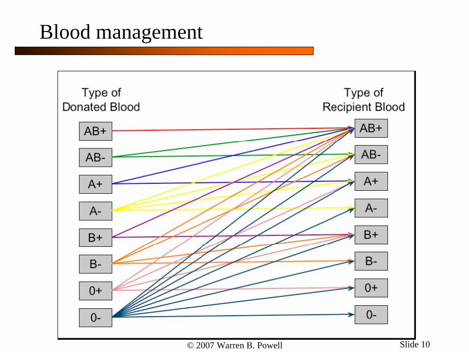
Blood management
© 2007 Warren B. Powell Slide 11
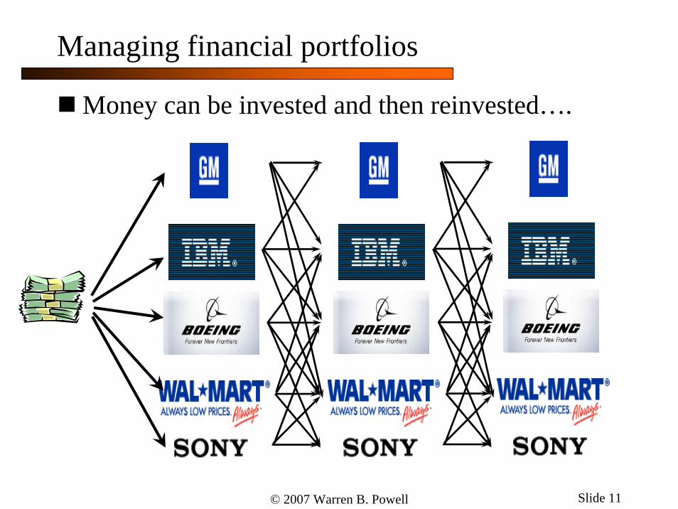
Managing financial portfolios
Money can be invested and then reinvested….

© 2007 Warren B. Powell Slide 12
Energy management
Applications• Jet fuel hedging – Designing strategies to hedge against
fluctuations in jet fuel (and other commodities).
• Valuing energy contracts
• Planning the use of future technologies
• R&D portfolio management
Research in ADP• Convergence proofs
• Rate of convergence research
• Design and evaluation of approximation strategies
• Design of advanced approximation strategies

© 2007 Warren B. Powell Slide 13
© 2007 Warren B. Powell Slide 14
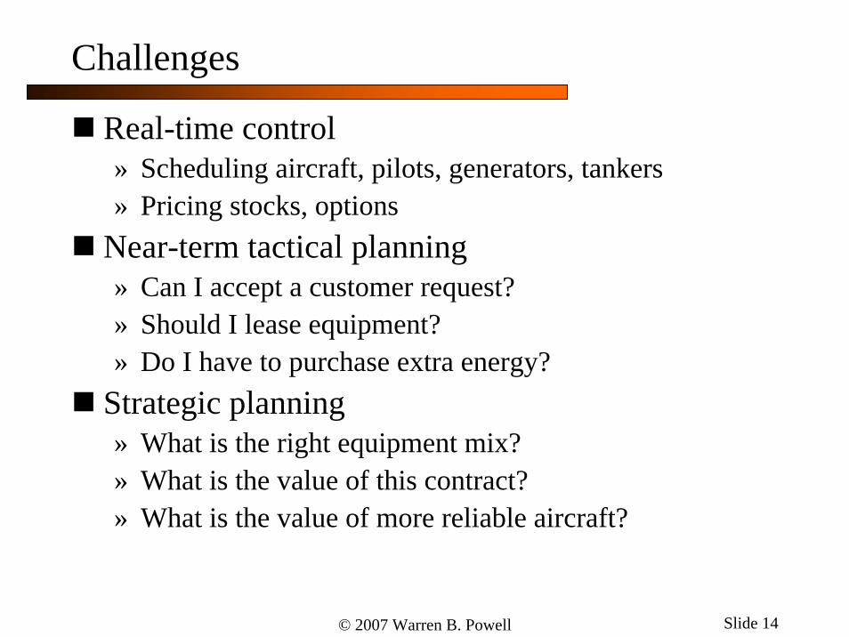
Challenges
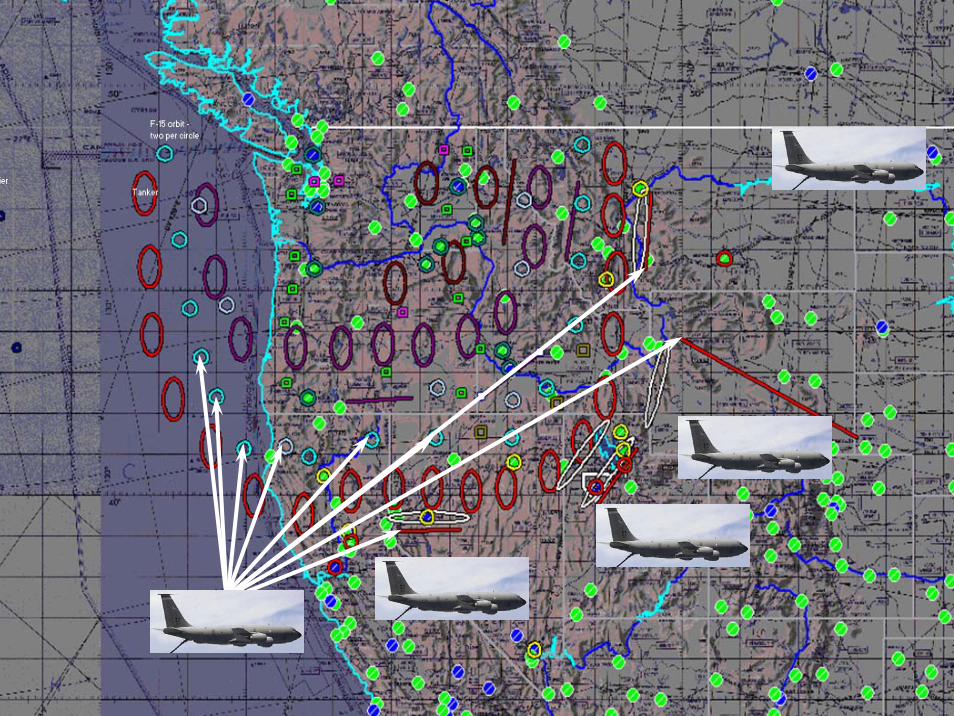
Real-time control» Scheduling aircraft, pilots, generators, tankers» Pricing stocks, options
Near-term tactical planning» Can I accept a customer request?» Should I lease equipment?» Do I have to purchase extra energy?
Strategic planning» What is the right equipment mix?» What is the value of this contract?» What is the value of more reliable aircraft?
© 2007 Warren B. Powell Slide 15
OutlineThe languages of dynamic programmingA resource allocation modelThe post-decision state variableExample: A discrete resource: the nomadic truckerThe states of our systemExample: A continuous resource: blood inventory managementApproximation methods» Lookup tables and aggregation» Basis functions
StepsizesExploration vs. exploitationApplications

© 2007 Warren B. Powell Slide 16
Languages
The languages of “optimization over time”
Engineering OR/AI/Probability OR/Math programming
DisciplineOptimal control
Markov decision processes
Stochastic programming
Decision (English) Control Action DecisionDecision (math) u a x"Value function" (English) Cost-to-go Value function Recourse function"Value function" (Math) J V QState variable x S Huh? (oh, "tenders")Optimality equations Hamilton-Jacobi Bellman Huh?
© 2007 Warren B. Powell Slide 17
Languages
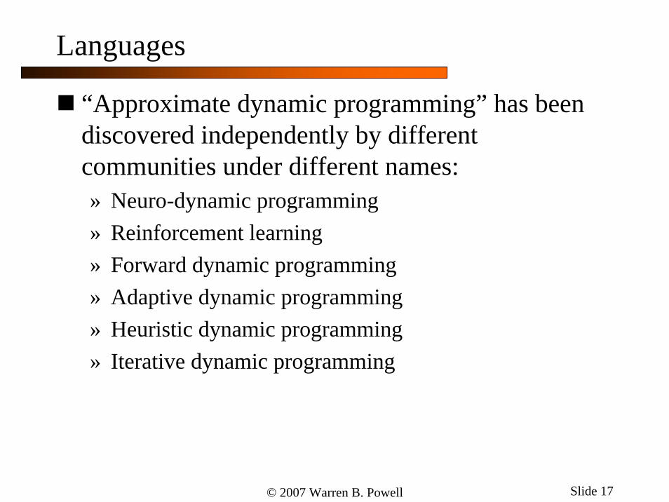
“Approximate dynamic programming” has been discovered independently by different communities under different names:» Neuro-dynamic programming» Reinforcement learning» Forward dynamic programming» Adaptive dynamic programming» Heuristic dynamic programming» Iterative dynamic programming

© 2007 Warren B. Powell Slide 18
Languages
How to land a plane:
» Control: angle, velocity, acceleration, pitch, yaw…» Noise: wind, measurement
( )( ) max ( , ) ( )V x C x u EV x= + 1 1t t u t t t t+ +

© 2007 Warren B. Powell Slide 19
Where to send a plane:
» Control: Where to send the plane to accomplish a goal.» Noise: demands on the system, equipment failures.
( )1 1( ) max ( , ) ( )t t a t t t tV S C S a EV S+ += +
Languages

© 2007 Warren B. Powell Slide 20
Languages
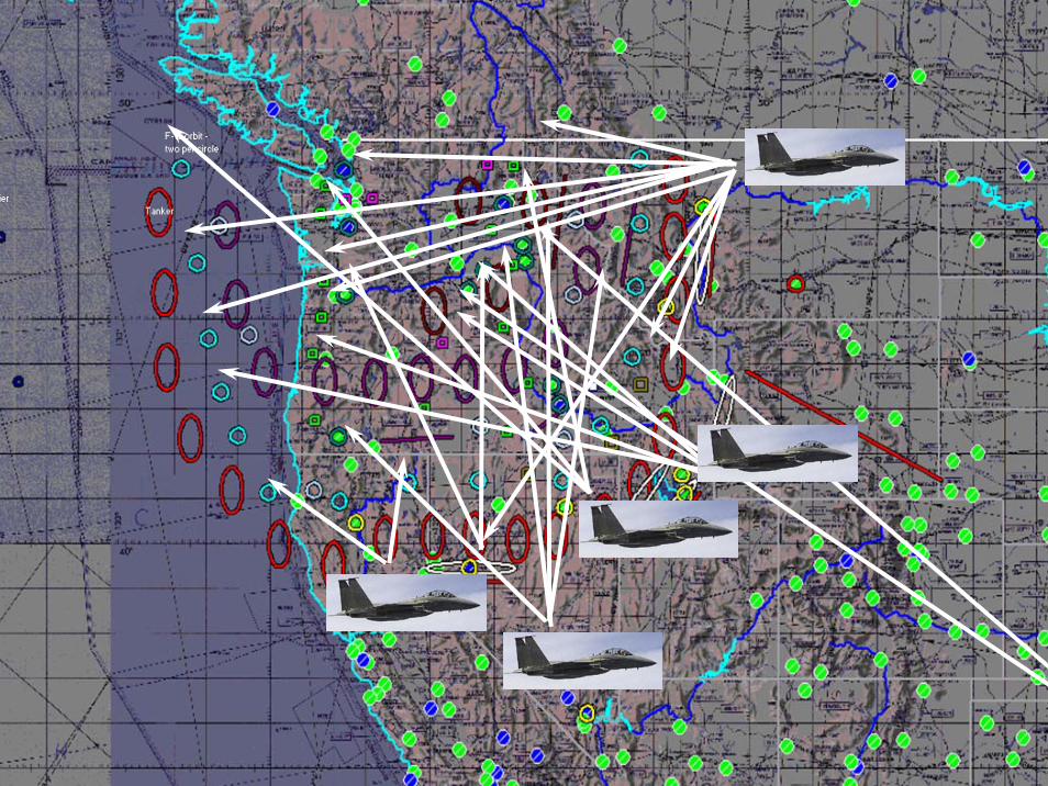
How to manage a fleet of aircraft:
» Control: Which plane to assign to each customer.» Noise: demands on the system, equipment failures.
( )1 1( ) max ( , ) ( )t t x t t t tV S C S x EV S+ += +

© 2007 Warren B. Powell Slide 21
A progression of models
Major problem classes
Simple attributes Complex attributes
Single entity Textbook Markov decision process
Classical AI applications
Multiple entities Classical OR applications
Opportunity for combining
AI/OR

© 2007 Warren B. Powell Slide 22
Sample applications
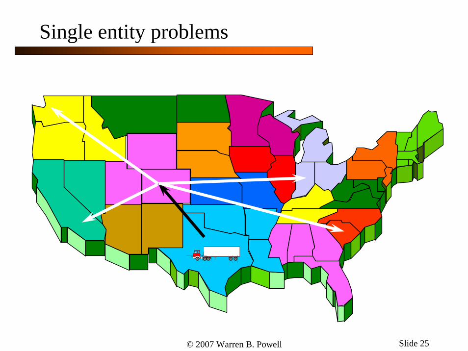
Single entity problems» Playing a board game» Routing a truck around the country» Planning a set of courses through college
Storage problems (single resource class)» Maintaining product inventories» Purchasing commodity futures (oil, orange juice, …)
Managing multiple resource classes» Blood inventories» Fleet management (with different equipment types)
Managing multiple, discrete resources» Locomotives, jets, people

© 2007 Warren B. Powell Slide 23
Single entity problems

© 2007 Warren B. Powell Slide 24
Single entity problems
© 2007 Warren B. Powell Slide 25
Single entity problems

© 2007 Warren B. Powell Slide 26
Single entity problems

© 2007 Warren B. Powell Slide 27
Single entity problems
© 2007 Warren B. Powell Slide 28
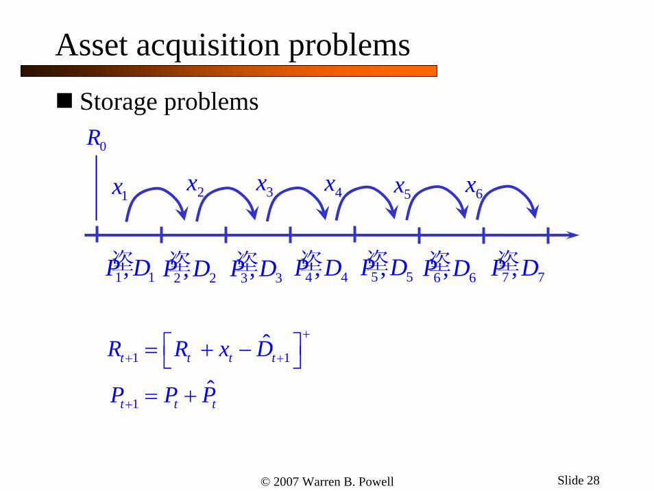
Asset acquisition problems
Storage problems
1 1垐,P D
1x
2 2垐,P D
2x 3x
3 3垐,P D
4x
4 4垐,P D
5x
5 5垐,P D
6x
6 6垐,P D 7 7
垐,P D
0R
1 1
1
ˆ
ˆt t t t
t t t
R R x D
P P P
+
+ +
+
⎡ ⎤= + −⎣ ⎦
= +
© 2007 Warren B. Powell Slide 29
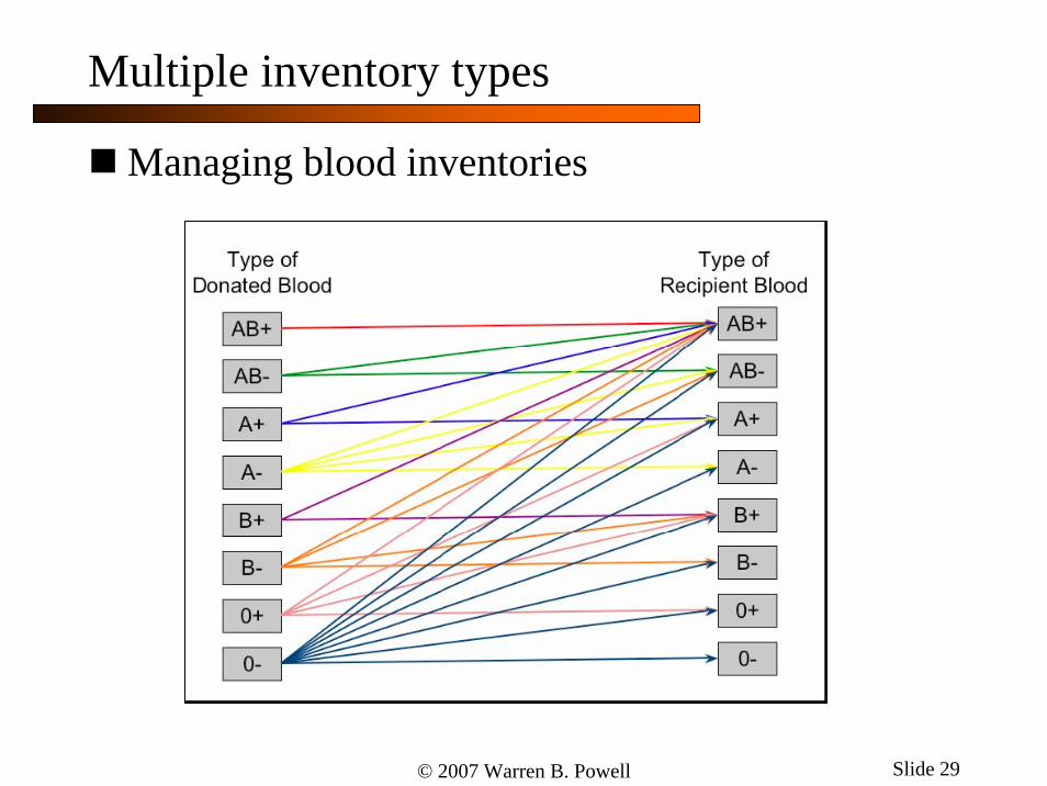
Multiple inventory types
Managing blood inventories

© 2007 Warren B. Powell Slide 30
Multiple inventory types
Managing blood inventories over time
Week 0 Week 1 Week 2

© 2007 Warren B. Powell Slide 31
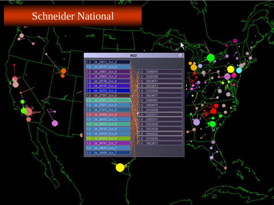
Schneider National
© 2007 Warren B. Powell Slide 32
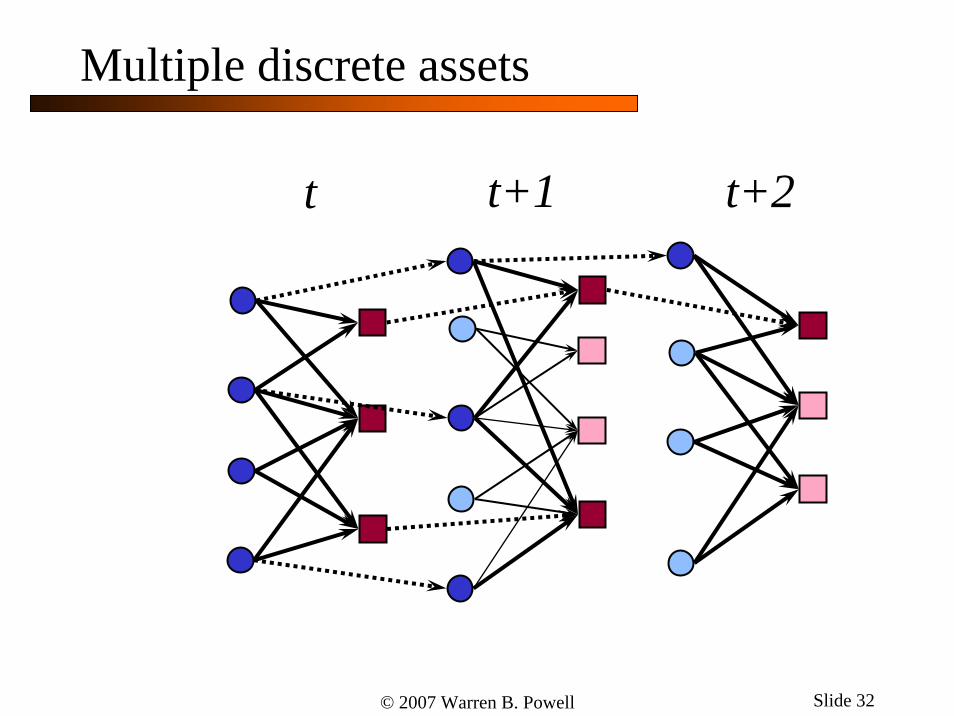
Multiple discrete assets
t t+1 t+2
© 2007 Warren B. Powell Slide 33
OutlineThe languages of dynamic programmingA resource allocation modelThe post-decision state variableExample: A discrete resource: the nomadic truckerThe states of our systemExample: A continuous resource: blood inventory managementApproximation methods» Lookup tables and aggregation» Basis functions
StepsizesExploration vs. exploitationApplications

© 2007 Warren B. Powell Slide 34
A resource allocation model
Modeling resources:» The state of a single resource:
» The state of multiple resources:
» The information process:
The attributes of a single resource The attribute space
aa=∈A
ˆ The change in the number of resources with attribute .
taRa
=
( )The number of resources with attribute
The resource state vectorta
t ta a
R a
R R∈
=
=A
© 2007 Warren B. Powell Slide 35
A resource allocation model
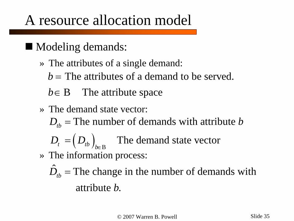
Modeling demands:» The attributes of a single demand:
» The demand state vector:
» The information process:
The attributes of a demand to be served. The attribute space
bb=∈B
( )The number of demands with attribute
The demand state vectortb
t tb b
D b
D D∈
=
=B
ˆ The change in the number of demands with attribute .
tbDb
=
© 2007 Warren B. Powell Slide 36
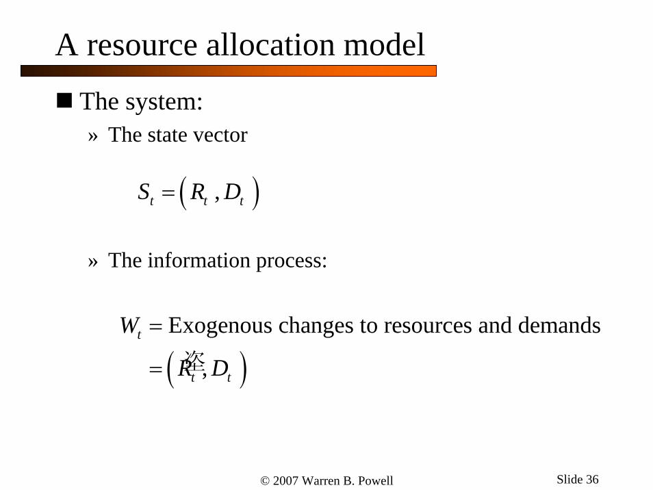
A resource allocation model
The system:» The state vector
» The information process:
( ),t t tS R D=
( )Exogenous changes to resources and demands垐,
t
t t
W
R D
=
=

© 2007 Warren B. Powell Slide 37
A resource allocation model
The three states of our system» The state of a single resource/entity
» The resource state vector
» The system state vector
1
2
3
t
t t
t
aa a
a
⎡ ⎤⎢ ⎥= ⎢ ⎥⎢ ⎥⎣ ⎦
1
2
3
ta
t ta
ta
R
R R
R
⎡ ⎤⎢ ⎥
= ⎢ ⎥⎢ ⎥⎣ ⎦
( ),t t tS R D=
© 2007 Warren B. Powell Slide 38
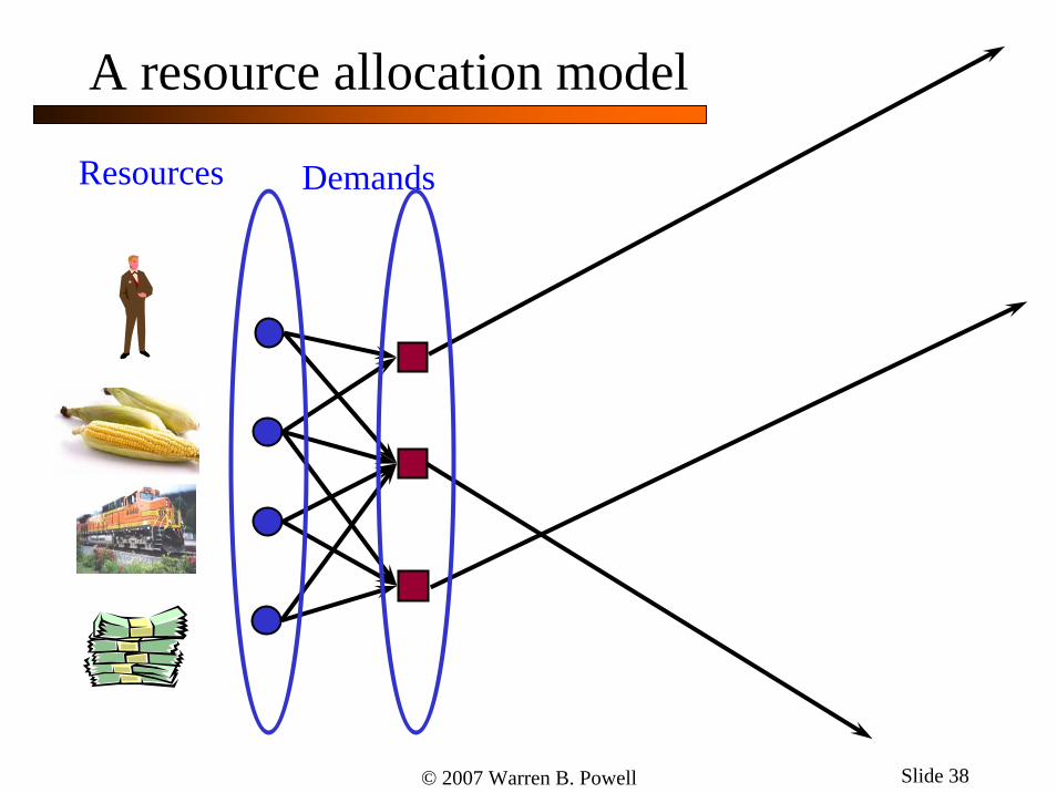
A resource allocation model
DemandsResources

© 2007 Warren B. Powell Slide 39
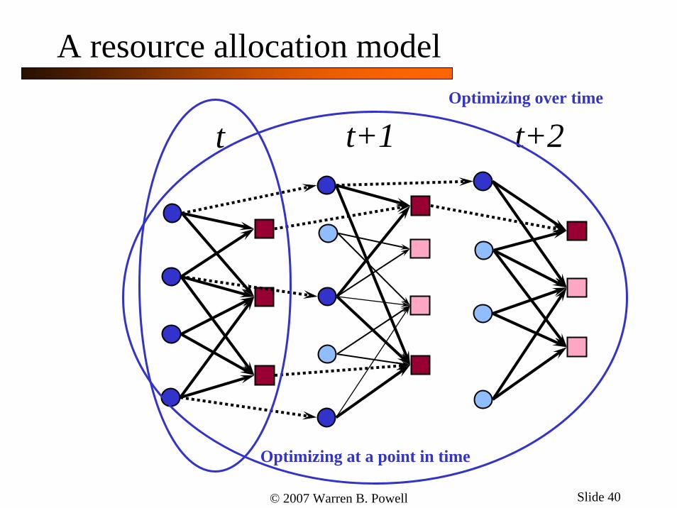
A resource allocation model
t t+1 t+2
© 2007 Warren B. Powell Slide 40
A resource allocation model
t t+1 t+2
Optimizing at a point in time
Optimizing over time
© 2007 Warren B. Powell Slide 41
OutlineThe languages of dynamic programmingA resource allocation modelThe post-decision state variableExample: A discrete resource: the nomadic truckerThe states of our systemExample: A continuous resource: blood inventory managementApproximation methods» Lookup tables and aggregation» Basis functions
StepsizesExploration vs. exploitationApplications
Do not use
weather report
Use w
eath
er re
port
Forecast sunny .6
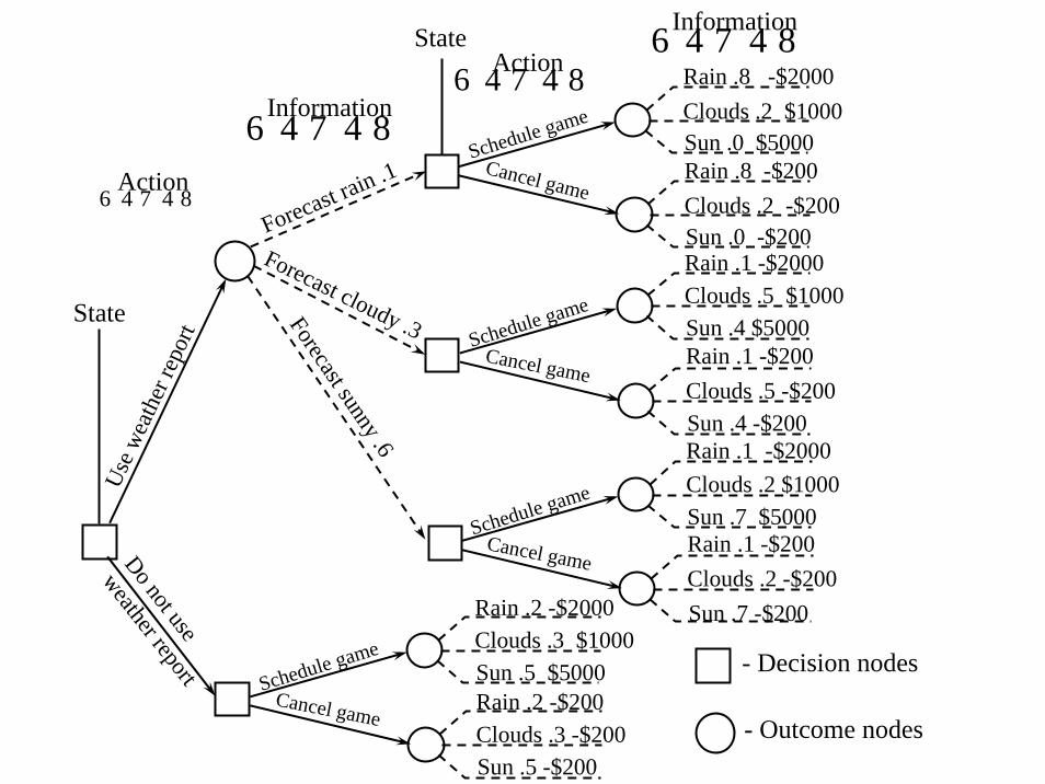
Rain .8 -$2000Clouds .2 $1000Sun .0 $5000Rain .8 -$200Clouds .2 -$200Sun .0 -$200
Schedule game
Cancel game
Rain .1 -$2000Clouds .5 $1000Sun .4 $5000Rain .1 -$200Clouds .5 -$200Sun .4 -$200
Schedule game
Cancel game
Rain .1 -$2000Clouds .2 $1000Sun .7 $5000Rain .1 -$200Clouds .2 -$200Sun .7 -$200
Schedule game
Cancel game
Rain .2 -$2000Clouds .3 $1000Sun .5 $5000Rain .2 -$200Clouds .3 -$200Sun .5 -$200
Schedule game
Cancel game
Forecast cloudy .3
Forecast rain .1
- Decision nodes
- Outcome nodes
Information6 4 7 4 8
Action6 4 7 4 8
Information6 4 7 4 8
Action6 4 7 4 8
State
State
© 2007 Warren B. Powell Slide 43
Laying the foundation
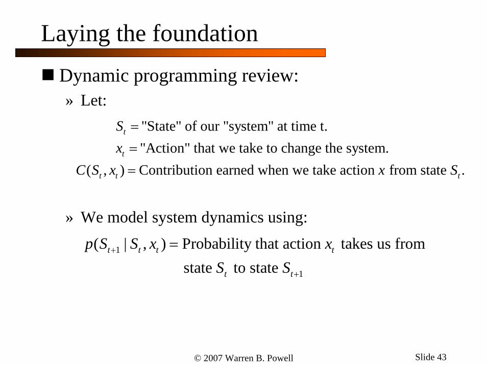
Dynamic programming review:» Let:
» We model system dynamics using:
"State" of our "system" at time t. "Action" that we take to change the system.
( , ) Contribution earned when we take action from state .
t
t
t t t
Sx
C S x x S
==
=
1
1
( | , ) Probability that action takes us from state to state
t t t t
t t
p S S x xS S
+
+
=

© 2007 Warren B. Powell Slide 44
Laying the foundation
Bellman’s equation:» Standard form:
» Expectation form:
1 1'
( ) max ( , ) ( ' | , ) ( ') t t x t t t t t t ts
V S C S x p s S x V S s+ +⎛ ⎞= + =⎜ ⎟⎝ ⎠
∑
( ){ }( )1 1( ) max ( , ) ( , ) | t t x t t t t t t t tV S C S x E V S S x S+ += +

Do not use
weather report
Use w
eath
er re
port
Forecast sunny .6
Rain .8 -$2000Clouds .2 $1000Sun .0 $5000Rain .8 -$200Clouds .2 -$200Sun .0 -$200
Schedule game
Cancel game
Rain .1 -$2000Clouds .5 $1000Sun .4 $5000Rain .1 -$200Clouds .5 -$200Sun .4 -$200
Schedule game
Cancel game
Rain .1 -$2000Clouds .2 $1000Sun .7 $5000Rain .1 -$200Clouds .2 -$200Sun .7 -$200
Schedule game
Cancel game
Rain .2 -$2000Clouds .3 $1000Sun .5 $5000Rain .2 -$200Clouds .3 -$200Sun .5 -$200
Schedule game
Cancel game
Forecast cloudy .3
Forecast rain .1
- Decision nodes
- Outcome nodes

Do not use
weather report
Use w
eath
er re
port
Forecast sunny .6
Schedule game
Cancel game
Schedule game
Cancel game
Schedule game
Cancel game
Schedule game
Cancel game
Forecast cloudy .3
Forecast rain .1
-$200
-$1400
-$200
$2300
-$200
$3500
$2400
-$200

Do not use
weather report
Use w
eath
er re
port
Forecast sunny .6Schedule game
Cancel game
Forecast cloudy .3
Forecast rain .1 -$200
$2300
$3500
$2400
-$200
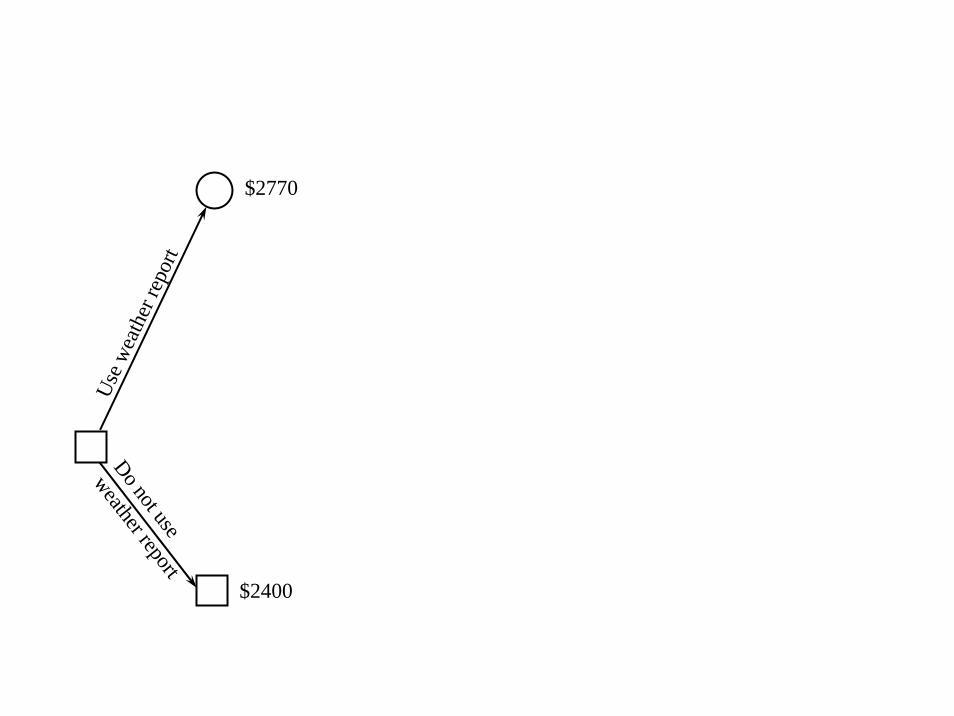
Do not use
weather report
Use w
eath
er re
port
$2770
$2400
© 2007 Warren B. Powell Slide 49
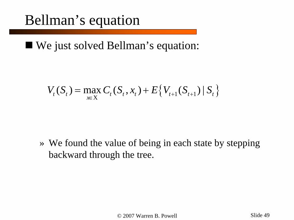
Bellman’s equation
We just solved Bellman’s equation:
» We found the value of being in each state by stepping backward through the tree.
{ }1 1( ) max ( , ) ( ) |t t t t t t t txV S C S x E V S S+ +∈
= +X

© 2007 Warren B. Powell Slide 50
Bellman’s equation
The challenge of dynamic programming:
Problem: Curse of dimensionality
{ }( )1 1( ) max ( , ) ( ) |t t t t t t t txV S C S x E V S S+ +∈
= +X

© 2007 Warren B. Powell Slide 51
The curses of dimensionality
What happens if we apply this idea to our blood problem?» State variable is:
• The supply of each type of blood, along with its age
– 8 blood types– 6 ages– = 48 “blood types”
• The demand for each type of blood– 8 blood types
» Decision variable is how much of 48 blood types to supply to 8 demand types.
• 216- dimensional decision vector» Random information
• Blood donations by week (8 types)• New demands for blood (8 types)

© 2007 Warren B. Powell Slide 52
The curses of dimensionality
The challenge of dynamic programming:
Problem: Curse of dimensionality
{ }( )1 1( ) max ( , ) ( ) |t t t t t t t txV S C S x E V S S+ +∈
= +X
Three curses
State spaceOutcome spaceAction space (feasible region)
© 2007 Warren B. Powell Slide 53
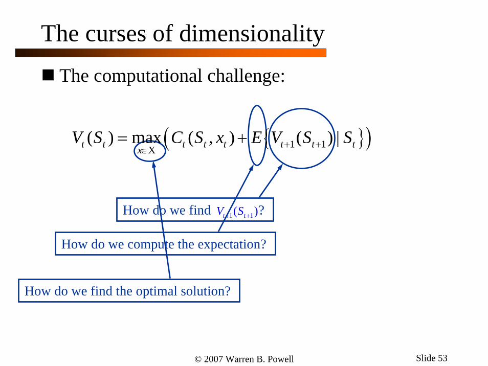
The curses of dimensionality
The computational challenge:
How do we find ? 1 1( )t tV S+ +
How do we compute the expectation?
How do we find the optimal solution?
{ }( )1 1( ) max ( , ) ( ) |t t t t t t t txV S C S x E V S S+ +∈
= +X

Do not
weath
Use w
eath
er re
port
Forecast sunny .6
Rain .8 -$2000Clouds .2 $1000Sun .0 $5000Rain .8 -$200Clouds .2 -$200Sun .0 -$200
Schedule game
Cancel game
Rain .1 -$2000Clouds .5 $1000Sun .4 $5000Rain .1 -$200Clouds .5 -$200Sun .4 -$200
Schedule game
Cancel game
Rain .1 -$2000Clouds .2 $1000Sun .7 $5000Rain .1 -$200Clouds .2 -$200S n 7 $200
Schedule game
Cancel game
Rain 2 -$2000
Forecast cloudy .3
Forecast rain .1
{ }( )1 1( ) max ( , ) ( ) |t t t t t t t txV S C S x E V S S+ +∈
= +X
tS
1tS +

Do not use
weather report
Use w
eath
er re
port
Forecast sunny .6
Rain .8 -$2000Clouds .2 $1000Sun .0 $5000Rain .8 -$200Clouds .2 -$200Sun .0 -$200
Schedule game
Cancel game
Rain .1 -$2000Clouds .5 $1000Sun .4 $5000Rain .1 -$200Clouds .5 -$200Sun .4 -$200
Schedule game
Cancel game
Rain .1 -$2000Clouds .2 $1000Sun .7 $5000Rain .1 -$200Clouds .2 -$200Sun .7 -$200
Schedule game
Cancel game
Rain .2 -$2000Clouds .3 $1000Sun .5 $5000Rain .2 -$200Clouds .3 -$200Sun .5 -$200
Schedule game
Cancel game
Forecast cloudy .3
Forecast rain .1
- Decision nodes
- Outcome nodes
© 2007 Warren B. Powell Slide 56
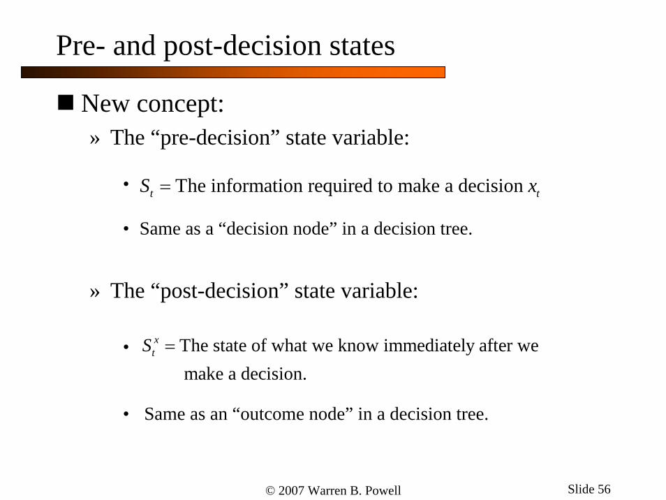
Pre- and post-decision states
New concept:» The “pre-decision” state variable:
•
• Same as a “decision node” in a decision tree.
» The “post-decision” state variable:
•
• Same as an “outcome node” in a decision tree.
The information required to make a decision t tS x=
The state of what we know immediately after we make a decision.
xtS =

© 2007 Warren B. Powell Slide 57
⎛⎜⎜⎜⎝
⎞⎟⎟⎟⎠
Pre- and post-decision states
Pre-decision, state-action, and post-decision
Pre-decision state State Action Post-decision state
93 states 93 9 state-action pairs× 93 states
© 2007 Warren B. Powell Slide 58
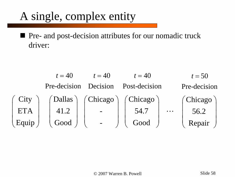
A single, complex entity
CityETAEquip
⎛ ⎞⎜ ⎟⎜ ⎟⎜ ⎟⎝ ⎠
Dallas41.2
Good
⎛ ⎞⎜ ⎟⎜ ⎟⎜ ⎟⎝ ⎠
40t =Pre-decision
Chicago54.7Good
⎛ ⎞⎜ ⎟⎜ ⎟⎜ ⎟⎝ ⎠
40t =Post-decision
Chicago56.2
Repair
⎛ ⎞⎜ ⎟⎜ ⎟⎜ ⎟⎝ ⎠
50t =Pre-decision
Pre- and post-decision attributes for our nomadic truck driver:
Chicago--
⎛ ⎞⎜ ⎟⎜ ⎟⎜ ⎟⎝ ⎠
Decision40t =
…
© 2007 Warren B. Powell Slide 59
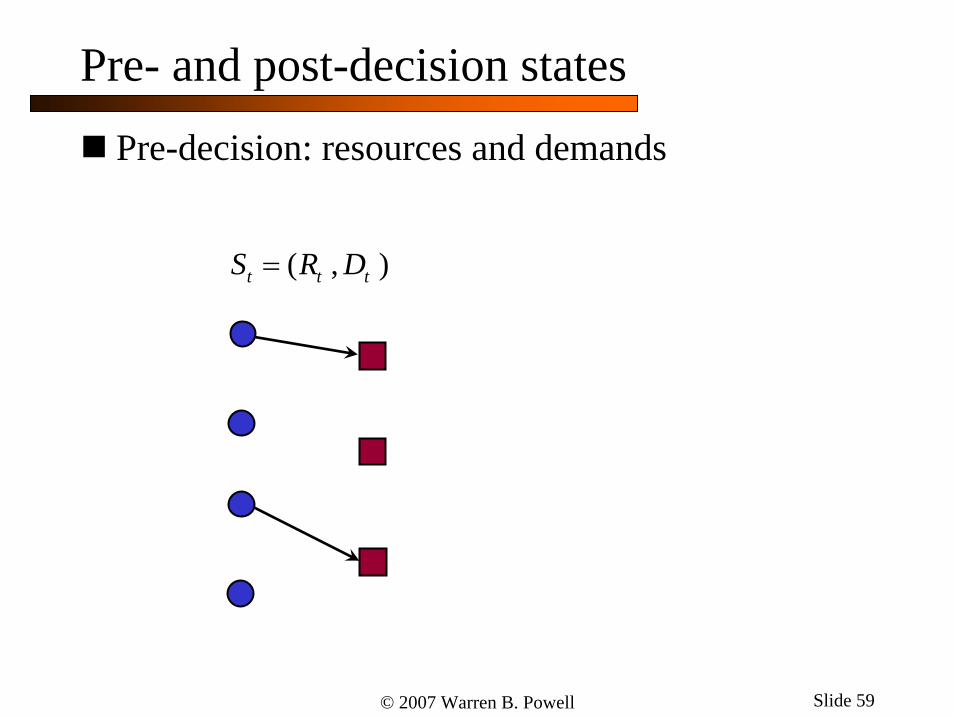
Pre- and post-decision states
( , )t t tS R D=
Pre-decision: resources and demands

© 2007 Warren B. Powell Slide 60
, ( , )x M xt t tS S S x=
Pre- and post-decision states

© 2007 Warren B. Powell Slide 61
Pre- and post-decision states
1 1 1垐( , )t t tW R D+ + +=
xtS ,
1 1( , )M W xt t tS S S W+ +=
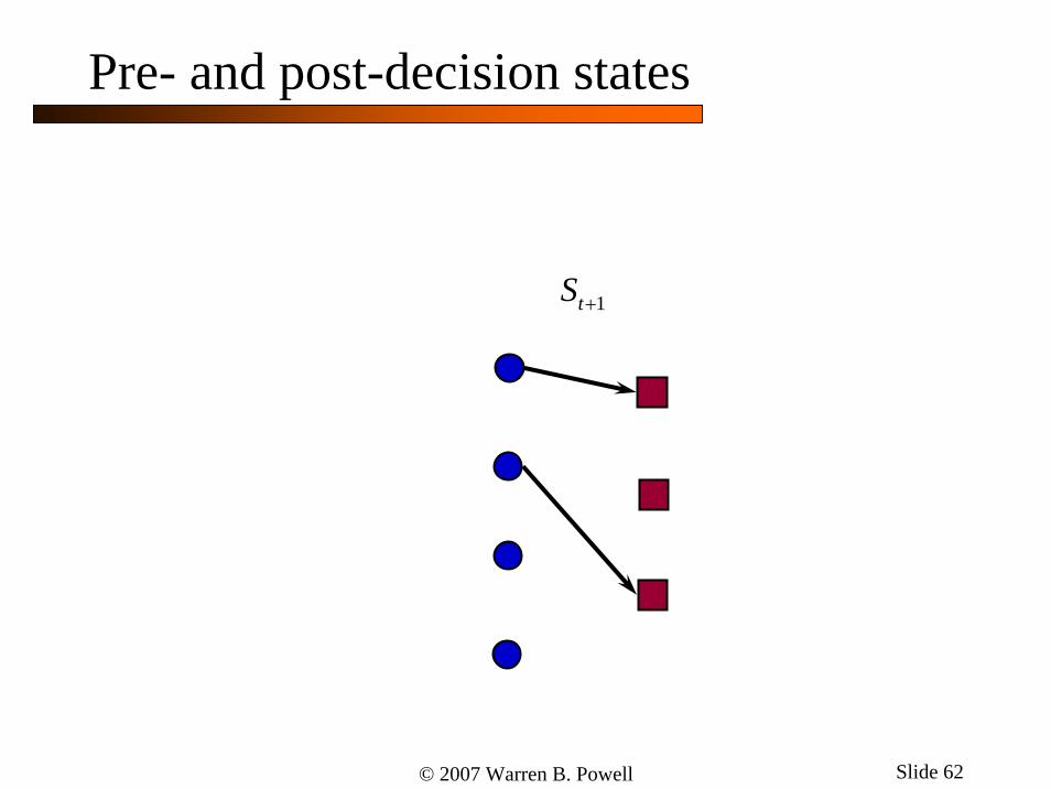
© 2007 Warren B. Powell Slide 62
Pre- and post-decision states
1tS +

© 2007 Warren B. Powell Slide 63
System dynamics
It is traditional to assume you are given the one-step transition matrix:
» Computing the transition matrix is impossible for the vast majority of problems.
We are going to assume that we are given a transition function:
» This is at the heart of any simulation model. » Often rule-based. Very easy to compute, even for large-scale
problems.
( )1 1, , Mt t t tS S S x W+ +=
1 1 ( | , ) Probability that action takes us from state to state t t t t t tp S S x x S S+ +=
© 2007 Warren B. Powell Slide 64
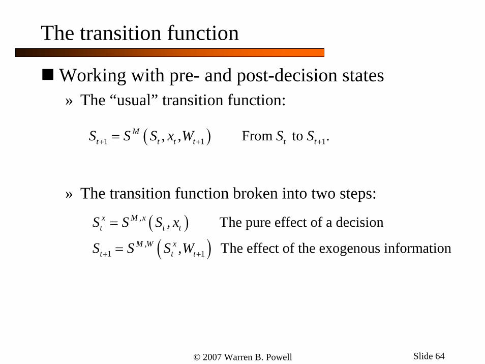
The transition function
Working with pre- and post-decision states» The “usual” transition function:
» The transition function broken into two steps:
( )( )
,
,1 1
, The pure effect of a decision
, The effect of the exogenous information
x M xt t t
M W xt t t
S S S x
S S S W+ +
=
=
( )1 1 1, , From to .Mt t t t t tS S S x W S S+ + +=

© 2007 Warren B. Powell Slide 65
The transition function
Actually, we have three transition functions:» The attribute transition function:
» The resource transition function
» The general transition function:
( )( )
,
,1 1
, The pure effect of a decision
, The effect of the exogenous information
x M xt t t
M W xt t t
a a a x
a a a W+ +
=
=
( )( )
,
,1 1
, The pure effect of a decision
, The effect of the exogenous information
x M xt t t
M W xt t t
S S S x
S S S W+ +
=
=
( )( )
,
,1 1
, The pure effect of a decision
, The effect of the exogenous information
x M xt t t
M W xt t t
R R R x
R R R W+ +
=
=

© 2007 Warren B. Powell Slide 66
Bellman’s equations with the post-decision state
Bellman’s equations broken into stages:
» Optimization problem (making the decision):
• Note: this problem is deterministic!
» Simulation problem (the effect of exogenous information):
( )( ),( ) max ( , ) ( , ) x M xt t x t t t t t t tV S C S x V S S x= +
{ },1 1( ) ( ( , )) |x x M W x x
t t t t t tV S E V S S W S+ +=
© 2007 Warren B. Powell Slide 67
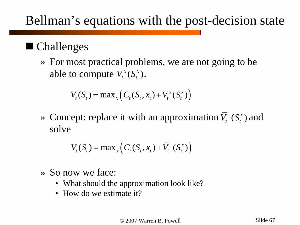
Bellman’s equations with the post-decision state
Challenges» For most practical problems, we are not going to be
able to compute .
» Concept: replace it with an approximation and solve
» So now we face:• What should the approximation look like?• How do we estimate it?
( )( ) max ( , ) ( ) x xt t x t t t t tV S C S x V S= +
( )x xt tV S
( )xt tV S
( )( ) max ( , ) ( ) xt t x t t t t tV S C S x V S= +
© 2007 Warren B. Powell Slide 68
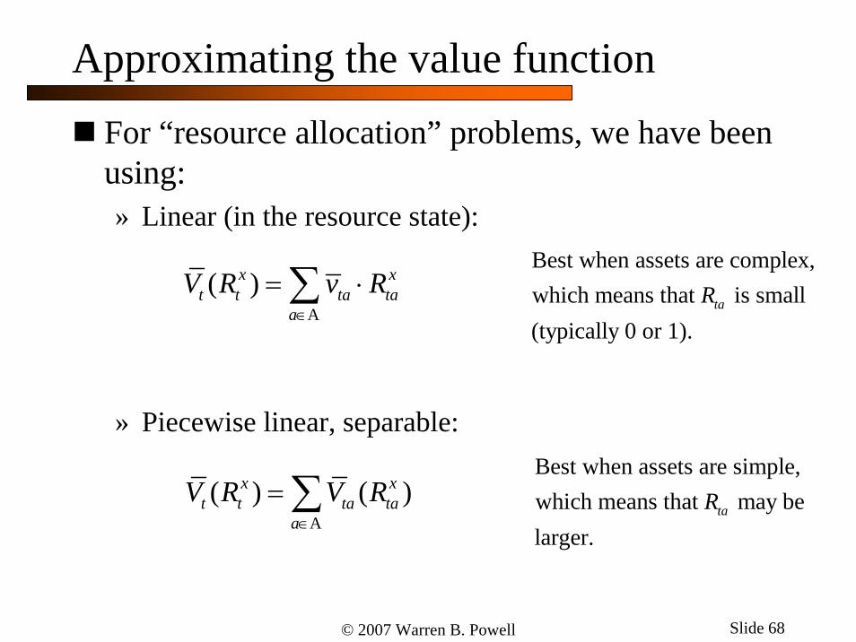
Approximating the value function
For “resource allocation” problems, we have been using:» Linear (in the resource state):
» Piecewise linear, separable:
( ) ( )x xt t ta ta
aV R V R
∈
= ∑A
Best when assets are complex,which means that is small(typically 0 or 1).
taR
Best when assets are simple,which means that may belarger.
taR
( )x xt t ta ta
aV R v R
∈
= ⋅∑A
© 2007 Warren B. Powell Slide 69
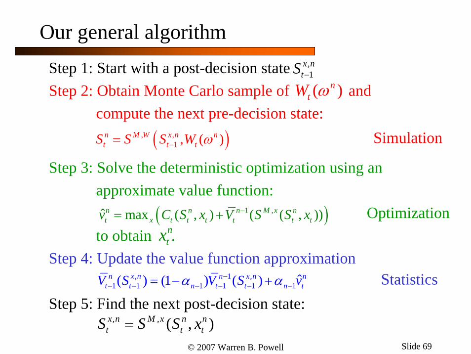
Our general algorithmStep 1: Start with a post-decision state Step 2: Obtain Monte Carlo sample of and
compute the next pre-decision state:
Step 3: Solve the deterministic optimization using anapproximate value function:
to obtain . Step 4: Update the value function approximation
Step 5: Find the next post-decision state:
, 1 ,1 1 1 1 1 1 ˆ( ) (1 ) ( )n x n n x n n
t t n t t n tV S V S vα α−− − − − − −= − +
( )1 ,ˆ max ( , ) ( ( , ) )n n n M x nt x t t t t t tv C S x V S S x−= +
ntx
( ), ,1 , ( )n M W x n n
t t tS S S W ω−=
,1
x ntS −
( )ntW ω
, , ( , )x n M x n nt t tS S S x=
Simulation
Optimization
Statistics

© 2007 Warren B. Powell Slide 70
Competing updating methods
Comparison to other methods:» Classical MDP (value iteration)
» Classical ADP (pre-decision state):
» Our method (update around post-decision state):
( ), 1 ,
, 1 ,1 1 1 1 1 1
ˆ max ( , ) ( ( , ))
ˆ( ) (1 ) ( )
n n x n M x nt x t t t t t t
n x n n x n nt t n t t n t
v C S x V S S x
V S V S vα α
−
−− − − − − −
= +
= − +
( )11( ) max ( , ) ( )n n
x tV S C S x EV S−+= +
( )11
'
11 1
ˆ max ( , ) ( ' | , ) '
ˆ( ) (1 ) ( )
n n n nt x t t t t t t
s
n n n n nt t n t t n t
v C S x p s S x V s
V S V S vα α
−+
−− −
⎛ ⎞= +⎜ ⎟⎝ ⎠
= − +
∑ˆ updates ( )t t tv V S
1 1ˆ updates ( )xt t tv V S− −
, 1x ntV −
© 2007 Warren B. Powell Slide 71
© 2007 Warren B. Powell Slide 72
OutlineThe languages of dynamic programmingA resource allocation modelThe post-decision state variableExample: A discrete resource: the nomadic truckerThe states of our systemExample: A continuous resource: blood inventory managementApproximation methods» Lookup tables and aggregation» Basis functions
StepsizesExploration vs. exploitationApplications

© 2007 Warren B. Powell Slide 73
The previous post-decision state: trucker in Texas
Nomadic trucker illustration
1 ( )=( )
xt
Location TXS
Time avail t−
⎛ ⎞ ⎛ ⎞= ⎜ ⎟ ⎜ ⎟⎝ ⎠ ⎝ ⎠

© 2007 Warren B. Powell Slide 74
Pre-decision state: we see the demands
$300
$150
$350
$450
Nomadic trucker illustration
ˆ( , )t t
TXS D
t⎛ ⎞
= ⎜ ⎟⎝ ⎠
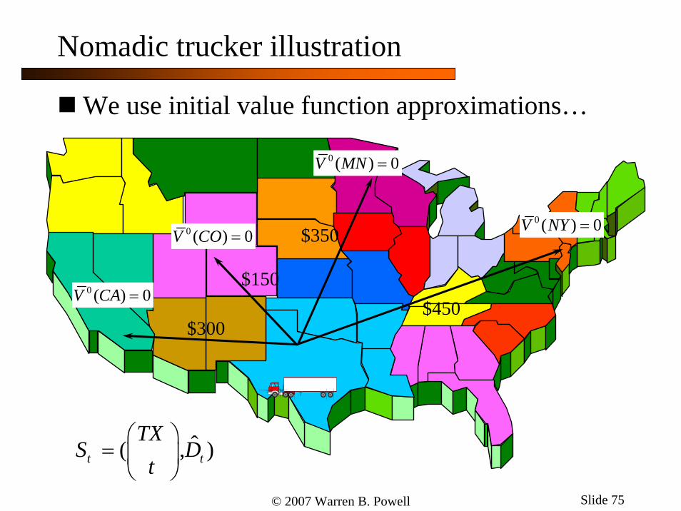
© 2007 Warren B. Powell Slide 75
We use initial value function approximations…
0 ( ) 0V CO =
0 ( ) 0V MN =
$300
$150
$350
$4500 ( ) 0V CA =
0 ( ) 0V NY =
Nomadic trucker illustration
ˆ( , )t t
TXS D
t⎛ ⎞
= ⎜ ⎟⎝ ⎠

© 2007 Warren B. Powell Slide 76
… and make our first choice:
$300
$150
$350
$450
0 ( ) 0V CO =
0 ( ) 0V CA =
0 ( ) 0V NY =
Nomadic trucker illustration1x
( )1
xt
NYS
t⎛ ⎞
= ⎜ ⎟+⎝ ⎠
0 ( ) 0V MN =

© 2007 Warren B. Powell Slide 77
Update the value of being in Texas.
1( ) 450V TX =
$300
$150
$350
$450
0 ( ) 0V CO =
0 ( ) 0V CA =
0 ( ) 0V NY =
Nomadic trucker illustration
( )1
xt
NYS
t⎛ ⎞
= ⎜ ⎟+⎝ ⎠
0 ( ) 0V MN =

© 2007 Warren B. Powell Slide 78
Now move to the next state, sample new demands and make a new decision
$600
$400
$180
$125
0 ( ) 0V CO =
0 ( ) 0V CA =
0 ( ) 0V NY =
1( ) 450V TX =
1 1ˆ( , )
1t t
NYS D
t
Nomadic trucker illustration
+ +
⎛ ⎞= ⎜ ⎟+⎝ ⎠
0 ( ) 0V MN =
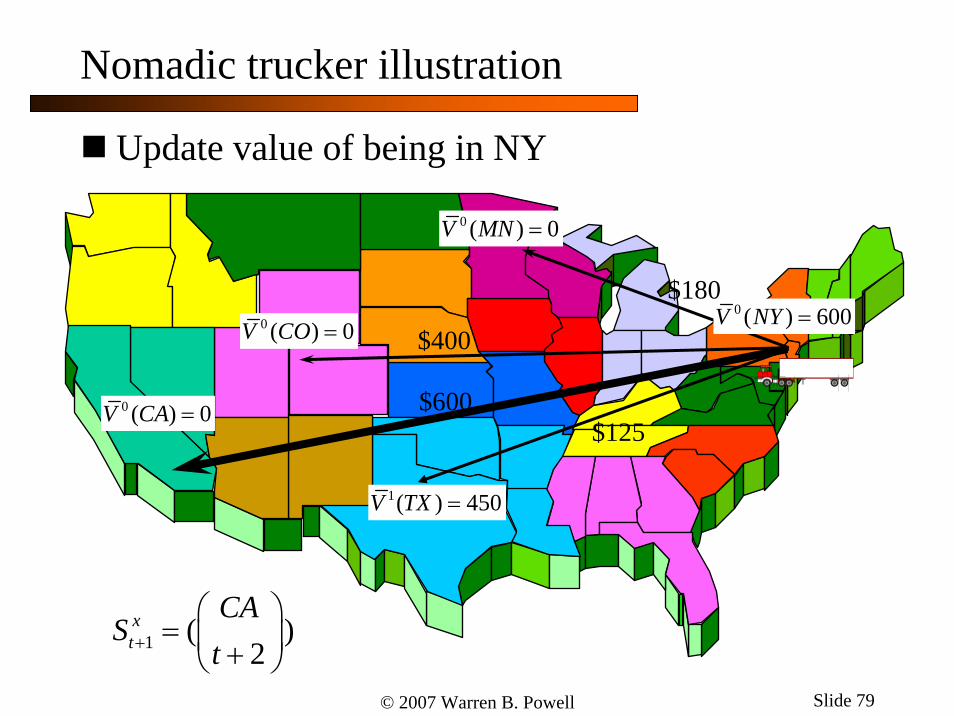
© 2007 Warren B. Powell Slide 79
Update value of being in NY
0 ( ) 600V NY =
$600
$400
$180
$125
0 ( ) 0V CO =
0 ( ) 0V CA =
1( ) 450V TX =
1 ( )2
xt
CAS
t+
⎛ ⎞= ⎜ ⎟+⎝ ⎠
Nomadic trucker illustration
0 ( ) 0V MN =
© 2007 Warren B. Powell Slide 80
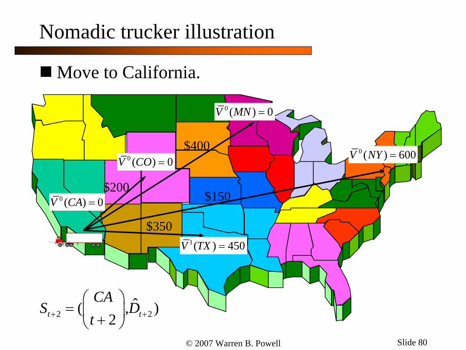
Move to California.
$150
$400
$200
$350
0 ( ) 0V CA =
0 ( ) 0V CO =
1( ) 450V TX =
Nomadic trucker illustration
0 ( ) 600V NY =
2 2ˆ( , )
2t t
CAS D
t+ +
⎛ ⎞= ⎜ ⎟+⎝ ⎠
0 ( ) 0V MN =
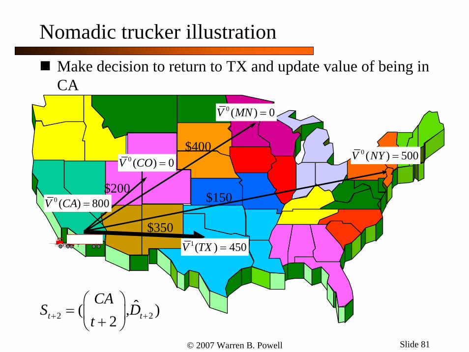
© 2007 Warren B. Powell Slide 81
Make decision to return to TX and update value of being in CA
$150
$400
$200
$350
0 ( ) 800V CA =
0 ( ) 0V CO =
1( ) 450V TX =
0 ( ) 500V NY =
2 2ˆ( , )
2t t
CAS D
t+ +
⎛ ⎞= ⎜ ⎟+⎝ ⎠
Nomadic trucker illustration
0 ( ) 0V MN =

© 2007 Warren B. Powell Slide 82
Back in TX, we repeat the process, observing a different set of demands.
1( ) 450V TX =
$275
$800
$385
$125
0 ( ) 0V CO =0 ( ) 500V NY =
Nomadic trucker illustration
0 ( ) 800V CA =
3 3ˆ( , )
3t t
TXS D
t+ +
⎛ ⎞= ⎜ ⎟+⎝ ⎠
0 ( ) 0V MN =

© 2007 Warren B. Powell Slide 83
We get a different decision and a new estimate of the value of being in TX
1( ) 450V TX =
0 ( ) 0V CO =
$275
$800
$385
$125
0 ( ) 500V NY =
Nomadic trucker illustration
0 ( ) 800V CA =
3 3ˆ( , )
3t t
TXS D
t+ +
⎛ ⎞= ⎜ ⎟+⎝ ⎠
0 ( ) 0V MN =

© 2007 Warren B. Powell Slide 84
Updating the value function:
1
2
2 1 2
Old value: ( ) $450
New estimate:ˆ ( ) $800
How do we merge old with new?ˆ ( ) (1 ) ( ) ( ) ( )
(0.90)$450+(0.10)$800 $485
V TX
v TX
V TX V TX v TXα α
=
=
= − +==
Nomadic trucker illustration

© 2007 Warren B. Powell Slide 85
An updated value of being in TX
1( ) 485V TX =
0 ( ) 0V CO =0 ( ) 600V NY =
$275
$800
$385
$125
Nomadic trucker illustration
0 ( ) 800V CA =
3 3ˆ( , )
3t t
TXS D
t+ +
⎛ ⎞= ⎜ ⎟+⎝ ⎠
0 ( ) 0V MN =

© 2007 Warren B. Powell Slide 86
OutlineThe languages of dynamic programmingA resource allocation modelThe post-decision state variableExample: A discrete resource: the nomadic truckerThe states of our systemExample: A continuous resource: blood inventory managementApproximation methods» Lookup tables and aggregation» Basis functions
StepsizesExploration vs. exploitationApplications

© 2007 Warren B. Powell Slide 87
The states of our system
Now let’s take a look at what we just did:
( )
Attribute of our nomadic trucker at time before the decision is made.
ˆ Vector of demands that are revealed at time .ˆ, Pre-decision state variable.
Attribute of our nomadic trucke
t
t
t t t
xt
a t
D t
S a D
a
=
=
=
= r at time after the decision is made.
Post-decision state variable.x xt t
t
S a=

© 2007 Warren B. Powell Slide 88
A single, complex entity
CityETAEquip
⎛ ⎞⎜ ⎟⎜ ⎟⎜ ⎟⎝ ⎠
Dallas41.2
Good
⎛ ⎞⎜ ⎟⎜ ⎟⎜ ⎟⎝ ⎠
40t =Pre-decision
Chicago54.7Good
⎛ ⎞⎜ ⎟⎜ ⎟⎜ ⎟⎝ ⎠
40t =Post-decision
Chicago56.2
Repair
⎛ ⎞⎜ ⎟⎜ ⎟⎜ ⎟⎝ ⎠
50t =Pre-decision
Pre- and post-decision attributes for our nomadic truck driver:
Chicago--
⎛ ⎞⎜ ⎟⎜ ⎟⎜ ⎟⎝ ⎠
Decision40t =
…

© 2007 Warren B. Powell Slide 89
Multiple, complex entities
Notation for multiple entities:» The truck state vector:
» The information process:
( )
The attributes of the truck The attribute space
The number of trucks with attribute
The truck state vector
truckta
truck truckt ta a
aa
R a
R R∈
=∈
=
=A
A
ˆ The change in the number of trucks with attribute .
trucktaR
a=

© 2007 Warren B. Powell Slide 90
Multiple, complex entities
Modeling the fleet management problem:» The load state vector:
» The information process:
( )
The attributes of a load to be moved. The attribute space
The number of tasks with attribute
The load state vector
loadtb
load loadt tb b
bb
R b
R R∈
=∈
=
=B
B
ˆ The change in the number of loads with attribute .
loadtbR
b=

© 2007 Warren B. Powell Slide 91
Multiple, complex entities
Modeling the fleet management problem:» The resource state vector (a.k.a. “physical state”)
» The information process:
( ),truck loadt t tR R R=
( )
ˆ The number of new arrivals (of drivers and loads) during time interval .
垐 ,
t
truck loadt t
t
Rt
R R
W
=
=
=

© 2007 Warren B. Powell Slide 92
The states of our system
The state of a single, simple entity:
a = [ ]Location
| | 100 10,000a∈ ≈ −A A |

© 2007 Warren B. Powell Slide 93
The states of our system
The state of a single, complex entity:
a =
TimeLocation
Equipment typeHome base
Operator attributesTime in serviceMaintenance status
⎡ ⎤⎢ ⎥⎢ ⎥⎢ ⎥⎢ ⎥⎢ ⎥⎢ ⎥⎢ ⎥⎢ ⎥⎢ ⎥⎣ ⎦
10 100 | | 10 10a∈ ≈ −A A |
The curse of dimensionality!
© 2007 Warren B. Powell Slide 94
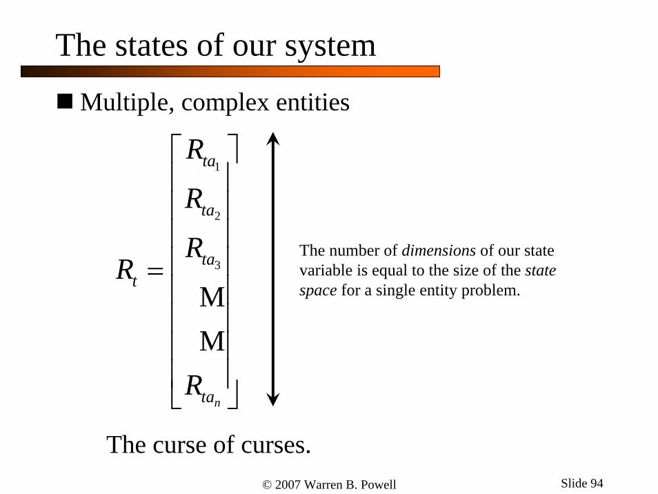
The states of our system
Multiple, complex entities
1
2
3
n
ta
ta
tat
ta
R
R
RR
R
⎡ ⎤⎢ ⎥⎢ ⎥⎢ ⎥⎢ ⎥=⎢ ⎥⎢ ⎥⎢ ⎥⎢ ⎥⎣ ⎦
MM
The number of dimensions of our state variable is equal to the size of the state space for a single entity problem.
The curse of curses.

© 2007 Warren B. Powell Slide 95
The states of our system
What is a state variable?
» A minimally dimensioned function of history that necessary and sufficient to compute the decision function, the transition function and the contribution function.

© 2007 Warren B. Powell Slide 96
The states of our system
The three states of our system» The state of a single resource/entity
» The state of all our resources
» The state of knowledge
1
2
3
t
t t
t
aa a
a
⎡ ⎤⎢ ⎥= ⎢ ⎥⎢ ⎥⎣ ⎦
1
2
3
ta
t ta
ta
R
R R
R
⎡ ⎤⎢ ⎥
= ⎢ ⎥⎢ ⎥⎣ ⎦
( ), Estimates of "other parameters"t t t tS R θ θ= =

© 2007 Warren B. Powell Slide 97
The states of our system
The state variable
( ), t t tS R θ=
The resource (physical) state
“Additional information”

© 2007 Warren B. Powell Slide 98
The states of our system
The state variable
( ), t t tS R θ=
The “state of knowledge”
© 2007 Warren B. Powell Slide 99
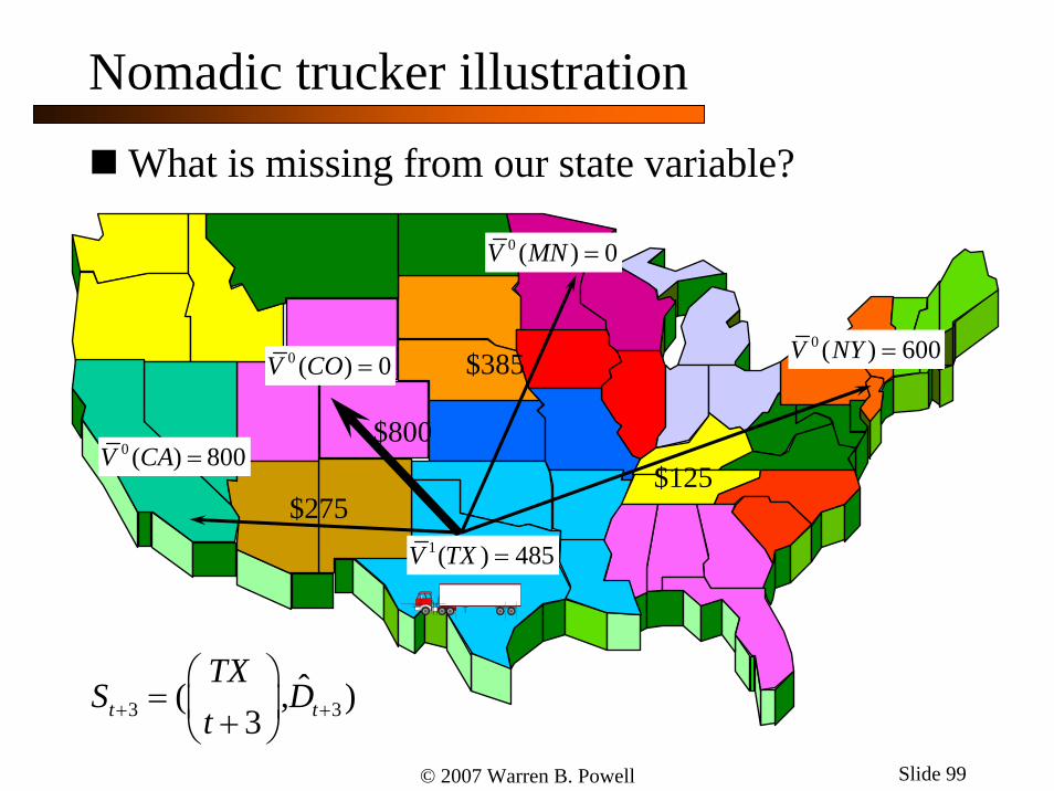
What is missing from our state variable?
1( ) 485V TX =
0 ( ) 0V CO =0 ( ) 600V NY =
$275
$800
$385
$125
Nomadic trucker illustration
0 ( ) 800V CA =
3 3ˆ( , )
3t t
TXS D
t+ +
⎛ ⎞= ⎜ ⎟+⎝ ⎠
0 ( ) 0V MN =
© 2007 Warren B. Powell Slide 100
OutlineThe languages of dynamic programmingA resource allocation modelThe post-decision state variableExample: A discrete resource: the nomadic truckerThe states of our systemExample: A continuous resource: blood inventory managementApproximation methods» Lookup tables and aggregation» Basis functions
StepsizesExploration vs. exploitationApplications

© 2007 Warren B. Powell Slide 101
Blood management
Managing blood inventories

© 2007 Warren B. Powell Slide 102
Blood management
Managing blood inventories over time
t=0
0S1 1垐,R D6 4 7 4 8
1S
Week 1
1x1xS
2 2垐,R D6 4 7 4 8
2S
Week 2
2x2xS
3 3垐,R D6 4 7 4 8
3S3x
Week 2
3xS
t=1 t=2 t=3

AB+,1
AB+,2
AB+,3
AB+,2
AB+,3
AB+,0
,ˆ
t ABD +
AB+,0
AB+,1
AB+,2
MAB-,0
AB-,1
AB-,2
M
M
,( ,0)t ABR +
,( ,1)t ABR +
,( ,2)t ABR +
,( ,0)t ABR −
,( ,1)t ABR −
,( ,2)t ABR −
,ˆ
t ABD −
,ˆ
t AD +
,ˆ
t ABD +
,ˆ
t ABD +
,ˆ
t ABD +
,ˆ
t ABD +
AB+
AB-
A+
A-
B+
B-
O+
O-
xtR
M
M
AB+,0
AB+,1
,ˆ
t ABD +
Satisfy a demand Hold
tS = ( )ˆ , t tR D

AB+,0
AB+,1
AB+,2
tR
MAB-,0
AB-,1
AB-,2
M
xtR
AB+,0
AB+,1
AB+,2
AB+,3
MAB+,0
AB+,1
AB+,2
AB+,3
Mˆ
tD
,( ,0)t ABR +
,( ,1)t ABR +
,( ,2)t ABR +
,( ,0)t ABR −
,( ,1)t ABR −
,( ,2)t ABR −

( )tF R
AB+,0
AB+,1
AB+,2
tR
MAB-,0
AB-,1
AB-,2
M
xtR
Mˆ
tD
,( ,0)t ABR +
,( ,1)t ABR +
,( ,2)t ABR +
,( ,0)t ABR −
,( ,1)t ABR −
,( ,2)t ABR −
Solve this as a linear program.
AB+,0
AB+,1
AB+,2
AB+,3
MAB+,0
AB+,1
AB+,2
AB+,3

( )tF R
AB+,0
AB+,1
AB+,2
tR
MAB-,0
AB-,1
AB-,2
M
xtR
Mˆ
tD
Duals
,( ,0)t̂ ABν +
,( ,1)t̂ ABν +
,( ,2)t̂ ABν +
,( ,0)t̂ ABν −
,( ,1)t̂ ABν −
,( ,2)t̂ ABν −
Dual variables give value additional unit of blood..
AB+,0
AB+,1
AB+,2
AB+,3
MAB+,0
AB+,1
AB+,2
AB+,3

© 2007 Warren B. Powell Slide 107
Updating the value function approximation
Estimate the gradient at
,( ,2)nt ABR +
,( ,2)ˆnt ABν +
ntR
( )tF R
© 2007 Warren B. Powell Slide 108
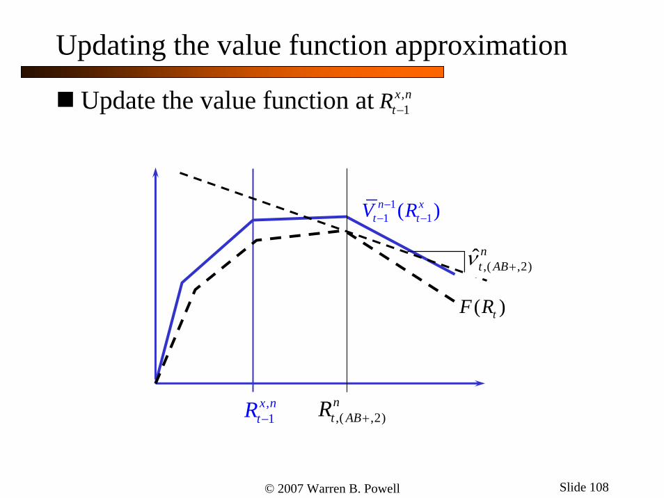
Updating the value function approximation
Update the value function at
,1
x ntR −
11 1( )n x
t tV R−− −
,1
x ntR −
,( ,2)ˆnt ABν +
( )tF R
,( ,2)nt ABR +

© 2007 Warren B. Powell Slide 109
Updating the value function approximation
Update the value function at ,1
x ntR −
,( ,2)ˆnt ABν +
,1
x ntR −
11 1( )n x
t tV R−− −

© 2007 Warren B. Powell Slide 110
Updating the value function approximation
Update the value function at ,1
x ntR −
,1
x ntR −
11 1( )n x
t tV R−− −
1 1( )n xt tV R− −
© 2007 Warren B. Powell Slide 111
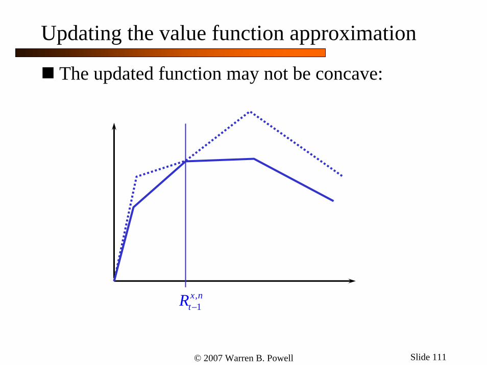
Updating the value function approximation
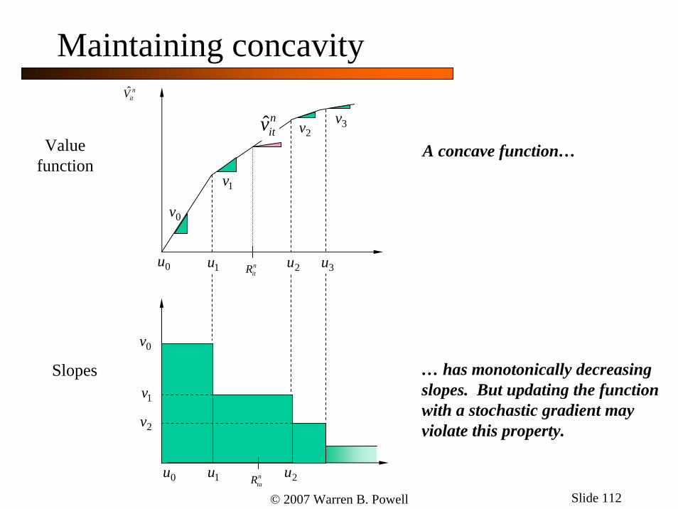
The updated function may not be concave:
,1
x ntR −
© 2007 Warren B. Powell Slide 112
0v
1v
ˆ nitV
2v 3v
Valuefunction
A concave function…
0v
1v
2v
0u 1u 2untaR
Slopes … has monotonically decreasing slopes. But updating the function with a stochastic gradient may violate this property.
0u 1u 2unitR 3u
Maintaining concavity
ˆnitv
© 2007 Warren B. Powell Slide 113
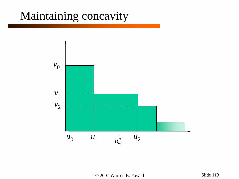
0v
1v
0u 1u 2untaR
2v
Maintaining concavity

© 2007 Warren B. Powell Slide 114
0v
1v
0u 1u 2untaR
ˆntav
2v
Maintaining concavity

© 2007 Warren B. Powell Slide 115
0v
1v
2v
0u 1u 2u
1 ˆ(1 )n n nta ta tav v vα α−= − +
ntaR
Maintaining concavity

© 2007 Warren B. Powell Slide 116
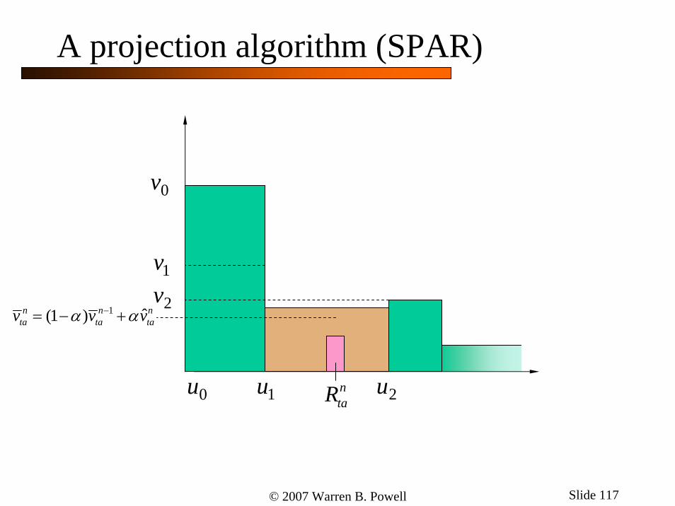
0v
1v
2v
0u 1u 2u
1 ˆ(1 )n n nta ta tav v vα α−= − +
ntaR
A projection algorithm (SPAR)
© 2007 Warren B. Powell Slide 117
0v
1v
2v
0u 1u 2u
1 ˆ(1 )n n nta ta tav v vα α−= − +
ntaR
A projection algorithm (SPAR)

© 2007 Warren B. Powell Slide 118
0v
1v
2v
0u 1u 2u
A projection algorithm (SPAR)
ntaR
1 ˆ(1 )n n nta ta tav v vα α−= − +
© 2007 Warren B. Powell Slide 119
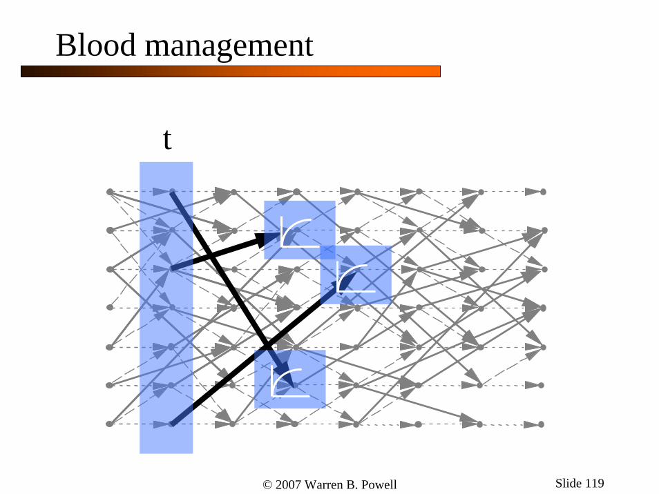
Blood management
t

© 2007 Warren B. Powell Slide 120
Blood management

© 2007 Warren B. Powell Slide 121
Blood management

© 2007 Warren B. Powell Slide 122
Blood management

© 2007 Warren B. Powell Slide 123
0
50
100
150
200
250
300
350
400
450
500
0 50 100 150 200
Iterations
Tota
l Sho
rtage
s (#
uni
ts)
Not UsingValueFunctions
Using ValueFunctions
Blood management

© 2007 Warren B. Powell Slide 124
OutlineThe languages of dynamic programmingA resource allocation modelThe post-decision state variableExample: A discrete resource: the nomadic truckerThe states of our systemExample: A continuous resource: blood inventory managementApproximation methods» Lookup tables and aggregation» Basis functions
StepsizesExploration vs. exploitationApplications

© 2007 Warren B. Powell Slide 125
Multiattribute resources
Assets can have a number of attributes:
LocationEquipment type
a
⎡ ⎤⎢ ⎥⎢ ⎥⎢ ⎥=⎢ ⎥⎢ ⎥⎢ ⎥⎣ ⎦
LocationETA
Equipment typeTrain priority
PoolDue for maint
Home shop
⎡ ⎤⎢ ⎥⎢ ⎥⎢ ⎥⎢ ⎥⎢ ⎥⎢ ⎥⎢ ⎥⎢ ⎥⎢ ⎥⎣ ⎦
LocationETA
A/C typeFuel level
Home shopCrewEqpt1
Eqpt100
⎡ ⎤⎢ ⎥⎢ ⎥⎢ ⎥⎢ ⎥⎢ ⎥⎢ ⎥⎢ ⎥⎢ ⎥⎢ ⎥⎢ ⎥⎢ ⎥⎢ ⎥⎢ ⎥⎣ ⎦
M
LocationETA
Bus. segmentSingle/team
DomicileDrive hoursDuty hours
8 day historyDays from home
⎡ ⎤⎢ ⎥⎢ ⎥⎢ ⎥⎢ ⎥⎢ ⎥⎢ ⎥⎢ ⎥⎢ ⎥⎢ ⎥⎢ ⎥⎢ ⎥⎢ ⎥⎣ ⎦
© 2007 Warren B. Powell Slide 126
Boxcars

© 2007 Warren B. Powell Slide 127
Multiattribute resources
The evolution of attributes:
≈A
TimeLocation
Boxcar typeTime to dest.
4,000
⎡ ⎤⎢ ⎥⎢ ⎥⎢ ⎥⎢ ⎥⎣ ⎦
1,680,000
a = TimeLocation⎡ ⎤⎢ ⎥⎣ ⎦
TimeLocation
Boxcar type
⎡ ⎤⎢ ⎥⎢ ⎥⎢ ⎥⎣ ⎦
40,000
TimeLocation
Boxcar typeTime to dest.Repair status
⎡ ⎤⎢ ⎥⎢ ⎥⎢ ⎥⎢ ⎥⎢ ⎥⎢ ⎥⎣ ⎦
5,040,000
TimeLocation
Boxcar typeTime to dest.Repair statusShipper pool
⎡ ⎤⎢ ⎥⎢ ⎥⎢ ⎥⎢ ⎥⎢ ⎥⎢ ⎥⎢ ⎥⎣ ⎦
50,400,000

© 2007 Warren B. Powell Slide 128
The states of our system
Multiple, complex entities
1
2
3
n
ta
ta
tat
ta
R
R
RR
R
⎡ ⎤⎢ ⎥⎢ ⎥⎢ ⎥⎢ ⎥=⎢ ⎥⎢ ⎥⎢ ⎥⎢ ⎥⎣ ⎦
MM
The number of dimensions of our state variable is equal to the size of the state space for a single entity problem.
The curse of curses.
© 2007 Warren B. Powell Slide 129
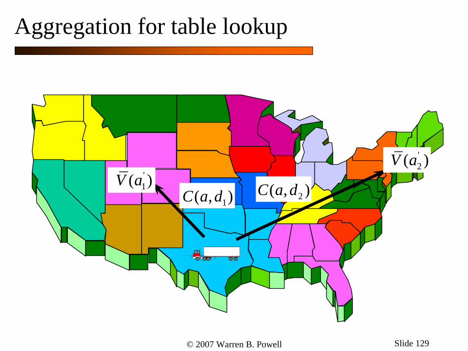
1( , )C a d 2( , )C a d'1( )V a
'2( )V a
Aggregation for table lookup

© 2007 Warren B. Powell Slide 130
NE regionPA
TX
?PAv =
NEv
PA NEv v≈
Aggregation for table lookup
© 2007 Warren B. Powell Slide 131
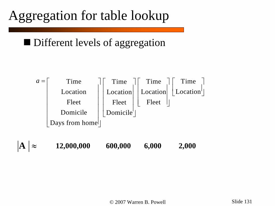
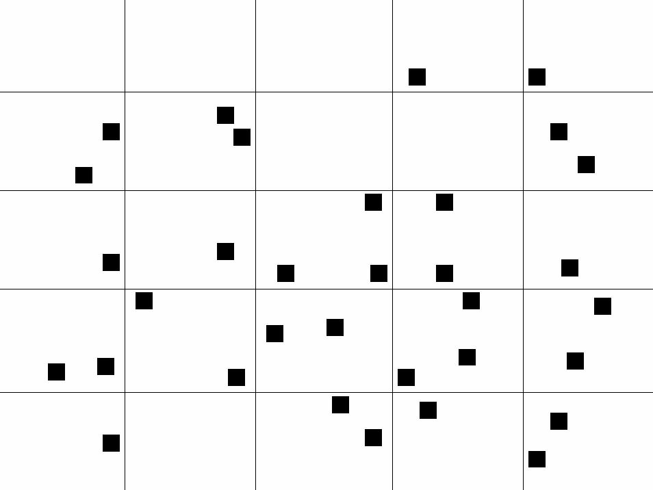
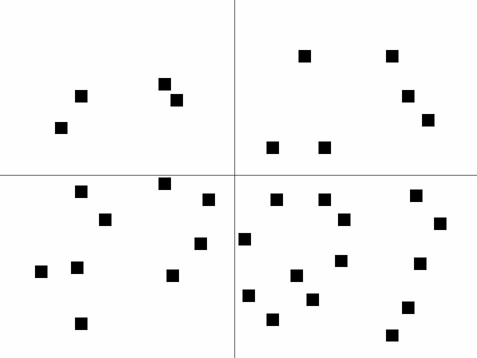
Different levels of aggregation
≈A
TimeLocation
FleetDomicile
⎡ ⎤⎢ ⎥⎢ ⎥⎢ ⎥⎢ ⎥⎣ ⎦
600,000
a =
2,000
TimeLocation⎡ ⎤⎢ ⎥⎣ ⎦
TimeLocation
Fleet
⎡ ⎤⎢ ⎥⎢ ⎥⎢ ⎥⎣ ⎦
6,000
TimeLocation
FleetDomicile
Days from home
⎡ ⎤⎢ ⎥⎢ ⎥⎢ ⎥⎢ ⎥⎢ ⎥⎢ ⎥⎣ ⎦
12,000,000
Aggregation for table lookup
© 2007 Warren B. Powell Slide 132
Aggregation
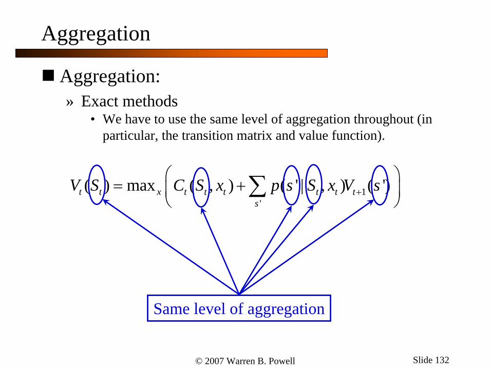
Aggregation:» Exact methods
• We have to use the same level of aggregation throughout (in particular, the transition matrix and value function).
1'
( ) max ( , ) ( ' | , ) ( ')t t x t t t t t ts
V S C S x p s S x V s+⎛ ⎞
= +⎜ ⎟⎝ ⎠
∑
Same level of aggregation

© 2007 Warren B. Powell Slide 133
Aggregation
Approximate DP» We only need to discretize the value function. We can
capture the full state variable in the transition function:• Decision function:
• Transition functions
( )arg max ( , ) ( ) xt x t t t t tx C S x V S= +
,1
,
( , ( ))
( , )
M W xt t tx M xt t t
S S S W
S S S x
ω−=
=
Value function using aggregated state
⎫⎪⎪⎬⎪⎪⎭
No aggregation

© 2007 Warren B. Powell Slide 134
Updating the value of a driver:
1 ˆ( ) (1 ) ( ) ( )n n
LocationLocation Location Fleet
v Fleet v Fleet v DomicileDomicile Domicile DOThrs
DaysFromHome
α α−
⎡ ⎤⎢ ⎥⎡ ⎤ ⎡ ⎤ ⎢ ⎥⎢ ⎥ ⎢ ⎥ ⎢ ⎥= − +⎢ ⎥ ⎢ ⎥ ⎢ ⎥⎢ ⎥ ⎢ ⎥⎣ ⎦ ⎣ ⎦ ⎢ ⎥⎢ ⎥⎣ ⎦
$2050 = $2000 $2500(1 0.10)− × + (0.10)
Value function Approximation may have fewer attributes than driver.
Drivers may have very detailed attributes
Aggregation for table lookup

© 2007 Warren B. Powell Slide 135
Estimating value functions» Most disaggregate level
1 ˆ( ) (1 ) ( ) ( )n n
LocationLocation Location Fleet
v Fleet v Fleet v DomicileDomicile Domicile DOThrs
DaysFromHome
α α−
⎡ ⎤⎢ ⎥⎡ ⎤ ⎡ ⎤ ⎢ ⎥⎢ ⎥ ⎢ ⎥ ⎢ ⎥= − +⎢ ⎥ ⎢ ⎥ ⎢ ⎥⎢ ⎥ ⎢ ⎥⎣ ⎦ ⎣ ⎦ ⎢ ⎥⎢ ⎥⎣ ⎦
Aggregation for table lookup

© 2007 Warren B. Powell Slide 136
Estimating value functions» Middle level of aggregation
1 ˆ( ) (1 ) ( ) ( )n n
LocationFleet
Location Locationv v v Domicile
Fleet FleetDOThrs
DaysFromHome
α α−
⎡ ⎤⎢ ⎥⎢ ⎥⎡ ⎤ ⎡ ⎤⎢ ⎥= − +⎢ ⎥ ⎢ ⎥⎢ ⎥⎣ ⎦ ⎣ ⎦⎢ ⎥⎢ ⎥⎣ ⎦
Aggregation for table lookup

© 2007 Warren B. Powell Slide 137
Estimating value functions» Most aggregate level
[ ] [ ]1 ˆ( ) (1 ) ( ) ( )n n
LocationFleet
v Location v Location v DomicileDOThrs
DaysFromHome
α α−
⎡ ⎤⎢ ⎥⎢ ⎥⎢ ⎥= − +⎢ ⎥⎢ ⎥⎢ ⎥⎣ ⎦
Aggregation for table lookup

© 2007 Warren B. Powell Slide 140
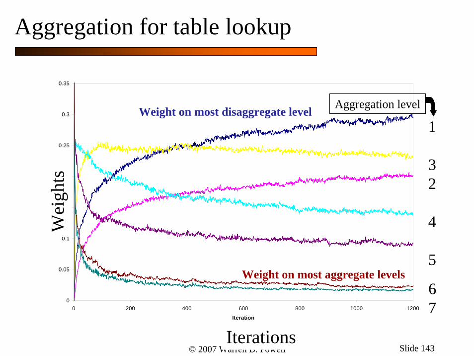
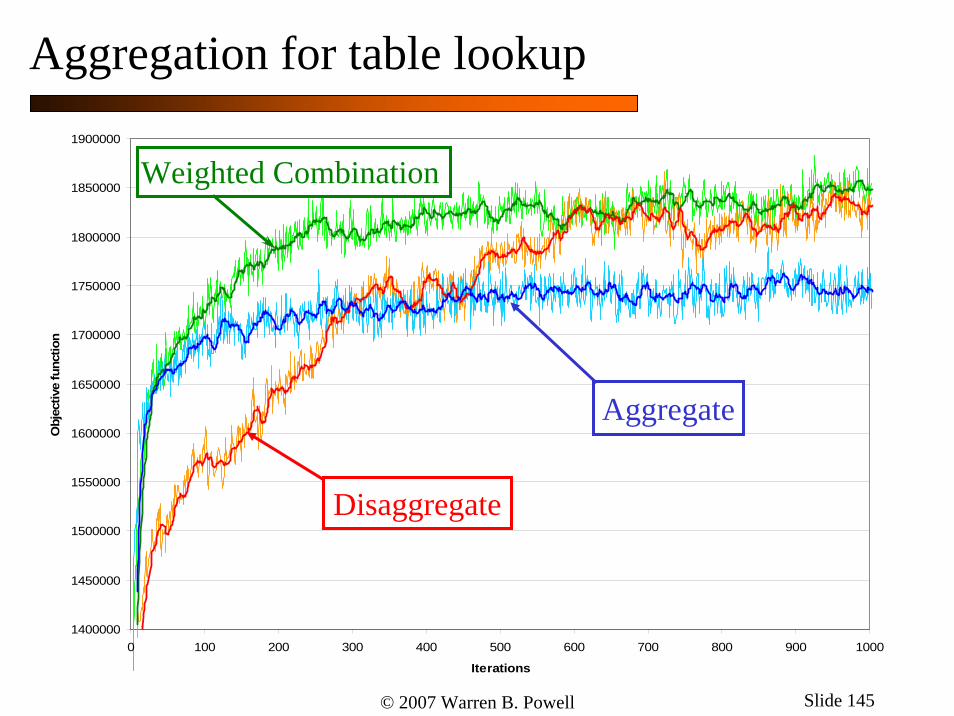
Using different levels of aggregation:» Pick the (single) level of aggregation that produces the best overall
results.» Pick the level of aggregation that produces the lowest variance for
each state.» Use a weighted sum of estimates at each level of aggregation
(weight depends only on the level of aggregation):
» Use a weighted sum, but where the weights depend on the state (attribute):
( , ) ( , )n g n g na a
gv w v=∑
( , ) ( , )n g n g na a a
gv w v=∑
Aggregation for table lookup


© 2007 Warren B. Powell Slide 142
State-dependent weighted aggregation:» There may be hundreds of thousands of weights, so
these have to be easy to compute.
( ) ( )( )
( ) ( ) ( )
12( ) ( ) ( )
1
where
g g ga a a a
g g
g g ga a a
v w v w
w Var v β−
= =
∝ +
∑ ∑
Estimate of variance Estimate of bias
Both can be computed using simple recursive formulas.
Aggregation for table lookup
© 2007 Warren B. Powell Slide 143
0
0.05
0.1
0.15
0.2
0.25
0.3
0.35
0 200 400 600 800 1000 1200
Iteration
Wei
ghts
Iterations
Wei
ghts
1
32
4
5
Aggregation level
67
Weight on most disaggregate level
Weight on most aggregate levels
Aggregation for table lookup
© 2007 Warren B. Powell Slide 144
1400000
1450000
1500000
1550000
1600000
1650000
1700000
1750000
1800000
1850000
1900000
0 100 200 300 400 500 600 700 800 900 1000
Iterations
Obj
ectiv
e fu
nctio
n
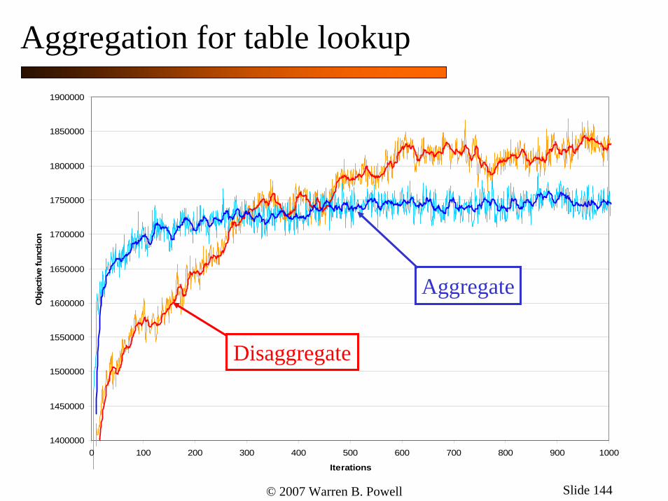
Aggregate
Disaggregate
Aggregation for table lookup
© 2007 Warren B. Powell Slide 145
1400000
1450000
1500000
1550000
1600000
1650000
1700000
1750000
1800000
1850000
1900000
0 100 200 300 400 500 600 700 800 900 1000
Iterations
Obj
ectiv
e fu
nctio
n
Weighted Combination
Aggregate
Disaggregate
Aggregation for table lookup
© 2007 Warren B. Powell Slide 146
OutlineThe languages of dynamic programmingA resource allocation modelThe post-decision state variableExample: A discrete resource: the nomadic truckerThe states of our systemExample: A continuous resource: blood inventory managementApproximation methods» Lookup tables and aggregation» Basis functions
StepsizesExploration vs. exploitationApplications

© 2007 Warren B. Powell Slide 147
Basis functions
Aggregation works well when we have a state (attribute) space with very little structure.But what if we have some structure? Consider our inventory problem:
1D̂
1x
2D̂
2x 3x
3D̂
4x
4D̂
5x
5D̂
6x
6D̂ 7D̂
( ) arg m ( )ax xn D Ot x t tt tx px Vcx R= − +
xtR

© 2007 Warren B. Powell Slide 148
Basis functions
Approximating the value function:» We have to exploit the structure of the value function
(e.g. concavity).» We might approximate the value function using a
simple polynomial
» .. or a complicated one:
» Sometimes, they get really messy:
20 1 2( | )t t t tV R R Rθ θ θ θ= + +
( )20 1 2 3 4( | ) ln sin( )t t t t t tV R R R R Rθ θ θ θ θ θ= + + + +

2 3(0) (1) (1)
, ' , ' , ' , '' '
(2) 2 (2) 2, ' , ' , ' , '
' '
2(3)
, , ''
21 1(4)
, ' , ' '' ' '
( | )
1
12
t t
t t st t st t wt t wts t t w t t
t wt t wt t st t stw t s t
ts t st t s ts s
t t
ts t st t s ts t t s t t
V R R R
R R
R RS
R RS
θ θ θ θ
θ θ
θ
θ
+ +
= =
+ +
= =
= + +
+ +
⎛ ⎞+ −⎜ ⎟
⎝ ⎠
⎛ ⎞⎛ ⎞+ −⎜ ⎟⎜ ⎟
⎝ ⎠⎝ ⎠
+
∑∑ ∑∑
∑∑ ∑∑
∑ ∑
∑ ∑ ∑∑22 2
(5), ' , ' '
' ' '
( ,1), , ,
2( ,2), , , '
'
3 2( ,3), , ' , '
' '
( ,4), , '
'
13
t t
ts t st t s ts t t s t t
wst ws t wt t st
w s
tws
t ws t wt t stw s t t
t tws
t ws t wt t stw s t t t t
wst ws t wt
t
R RS
R R
R R
R R
R
θ
θ
θ
θ
θ
+ +
= =
+
=
+ +
= =
⎛ ⎞⎛ ⎞−⎜ ⎟⎜ ⎟
⎝ ⎠⎝ ⎠
+
⎛ ⎞+ ⎜ ⎟
⎝ ⎠⎛ ⎞⎛ ⎞+ ⎜ ⎟⎜ ⎟⎝ ⎠⎝ ⎠
+
∑ ∑ ∑∑
∑∑
∑∑ ∑
∑∑ ∑ ∑2 2
, ''
( ,5), , , 2 , , , 2
t t
t stw s t t t
wst sw t s t t wt t w t
w s
R
R R Rθ
+ +
= =
+ +
⎛ ⎞⎛ ⎞⎜ ⎟⎜ ⎟⎝ ⎠⎝ ⎠
+
∑∑ ∑ ∑
∑∑
1,2,3 4,5,6,7
8-14
15
16
17
18
19
20
21
22

© 2007 Warren B. Powell Slide 150
Basis functions
We can write a model of the observed value of being in a state as:
This is often written as a generic regression model:
The ADP community refers to the independent variables as basis functions:
( )20 1 2 3 4ˆ ln sin( )t t t tv R R R Rθ θ θ θ θ ε= + + + + +
0 1 1 2 2 3 3 4 4 Y X X X Xθ θ θ θ θ= + + + +
0 0 1 1 2 2 3 3 4 4( ) ( ) ( ) ( ) ( )
= ( )f ff
Y R R R R R
R
θ ϕ θ ϕ θ ϕ θ ϕ θ ϕ
θ ϕ∈
= + + + +
∑F
( )f Rϕ are also known as features.
© 2007 Warren B. Powell Slide 151
Basis functions
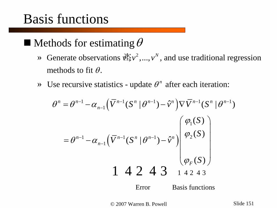
Methods for estimating»
»
θ1 2垐 �Generate observations , ,..., , and use traditional regression
methods to fit .
Nv v vθ
Use recursive statistics - update after each iteration:nθ
( )
( )
1 1 1 1 11
1
21 1 11
ˆ( | ) ( | )
( )( )
ˆ ( | )
( )
n n n n n n n n nn
n n n n nn
F
V S v V S
SS
V S v
S
θ θ α θ θ
ϕϕ
θ α θ
ϕ
− − − − −−
− − −−
= − − ∇
⎛ ⎞⎜ ⎟⎜ ⎟= − −⎜ ⎟⎜ ⎟⎝ ⎠
1 4 2 4 3Error
1 4 2 4 3
Basis functions

© 2007 Warren B. Powell Slide 152
Basis functions
Notes:» When using basis functions, we are basically drawing
on the entire field of statistics.» Designing basis functions (independent variables) is
mostly art.» In special cases, the resulting algorithm can produce
optimal solutions.» Most of the time, we are hoping for “good” solutions.» In some cases, it can work terribly.» As a general rule – you have to use problem structure.
Value function approximations have to capture the right structure. Blind use of polynomials will rarely be successful.
© 2007 Warren B. Powell Slide 153
OutlineThe languages of dynamic programmingA resource allocation modelThe post-decision state variableExample: A discrete resource: the nomadic truckerThe states of our systemExample: A continuous resource: blood inventory managementApproximation methods» Lookup tables and aggregation» Basis functions
StepsizesExploration vs. exploitationApplications

© 2007 Warren B. Powell Slide 154
Stepsizes
Stepsizes:» Fundamental to ADP is an updating equation that looks
like:
11 1 1 1 1 1 ˆ( ) (1 ) ( )n x n x n
t t n t t n tV S V S vα α−− − − − − −= − +
Old estimate New observationUpdated estimate
The stepsize“Learning rate”
“Smoothing factor”

© 2007 Warren B. Powell Slide 155
Stepsizes
Theory:» Many convergence results
require:
» For example:
Practice» 1/n “doesn’t work”» Constant stepsizes» Various stepsize rules
• Deterministic• Stochastic
( )
11
21
1
nn
nn
α
α
∞
−=
∞
−=
= ∞
< ∞
∑
∑
11
n nα − =

© 2007 Warren B. Powell Slide 156
Rate of convergence
Smoothed estimate using 1/n

© 2007 Warren B. Powell Slide 157
Rate of convergence
The challenge of stepsizes:» When have we converged?
1500000
1550000
1600000
1650000
1700000
1750000
1800000
1850000
1900000
1950000
2000000
0 100 200 300 400 500 600 700 800 900 1000
10001500000
1550000
1600000
1650000
1700000
1750000
1800000
1850000
1900000
1950000
2000000
0 10 20 30 40 50 60 70 80 90 100100
We need to improve our understanding of adaptive stepsizes.
100
© 2007 Warren B. Powell Slide 158
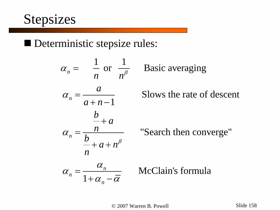
Stepsizes
Deterministic stepsize rules:1 1 or Basic averaging
Slows the rate of descent1
"Search then converge"
McClain's formula1
n
n
n
nn
n
n na
a nb an
b a nn
β
β
α
α
α
ααα α
=
=+ −
+=
+ +
=+ −
© 2007 Warren B. Powell Slide 159
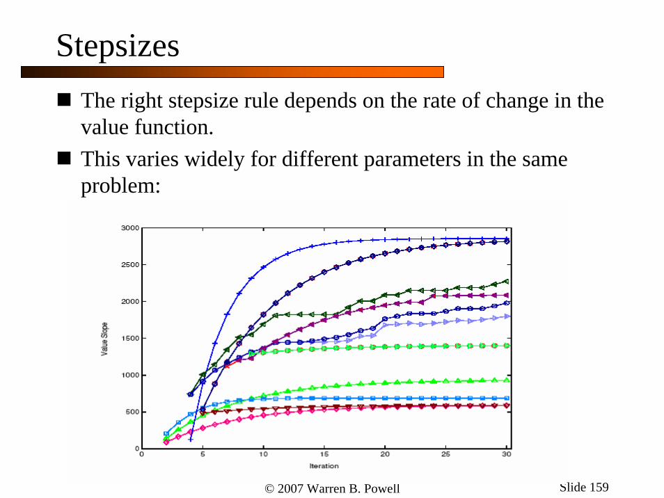
StepsizesThe right stepsize rule depends on the rate of change in the value function.This varies widely for different parameters in the same problem:

© 2007 Warren B. Powell Slide 160
StepsizesThe right stepsize rule depends on the rate of change in the value function.This varies widely for different parameters in the same problem:
Large stepsize

© 2007 Warren B. Powell Slide 161
StepsizesThe right stepsize rule depends on the rate of change in the value function.This varies widely for different parameters in the same problem:
Small stepsize
© 2007 Warren B. Powell Slide 162
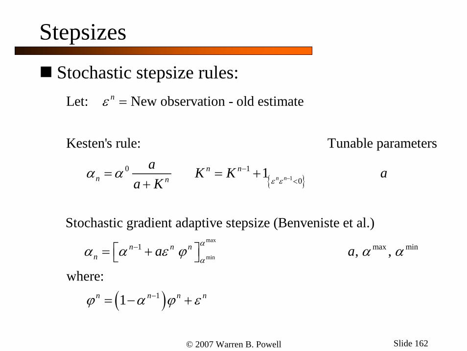
Stepsizes
Stochastic stepsize rules:
{ }1
max
min
0 10
1
Let: New observation - old estimate
Kesten's rule: Tunable parameters
1
Stochastic gradient adaptive stepsize (Benveniste et al.)
n n
n
n nn n
n n nn
a K K aa K
a
ε ε
α
α
ε
α α
α α ε ϕ
−−
<
−
=
= = ++
⎡ ⎤= +⎣ ⎦
( )
max min
1
, ,
where:
1n n n n
a α α
ϕ α ϕ ε−= − +

© 2007 Warren B. Powell Slide 163
Stepsizes
( ) ( )
( ) ( )
2
21 2
2 21
2
11
where:
1
As increases, stepsize decreasesAs increases, stepsize increases.
n n n
n nn n
n
σαλ σ β
λ α λ α
σ
β
−
−
= −+ +
= − +
Estimate of the variance
Estimate of the bias
Bias
Noise
Bias-adjusted Kalman filter
© 2007 Warren B. Powell Slide 164
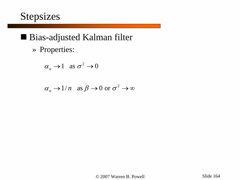
Stepsizes
Bias-adjusted Kalman filter» Properties:
2
2
1 as 0
1/ as 0 or
n
n n
α σ
α β σ
→ →
→ → →∞
© 2007 Warren B. Powell Slide 165
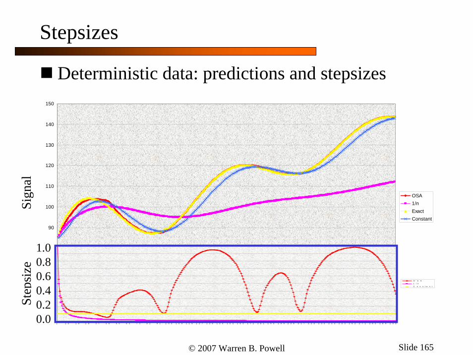
Stepsizes
Deterministic data: predictions and stepsizes
50
60
70
80
90
100
110
120
130
140
150
1 10 19 28 37 46 55 64 73 82 91 100 109 118 127 136 145 154 163 172 181 190 199 208 217 226 235 244 253 262 271 280 289 298
OSA1/nExactConstant
0
0 . 1
0 . 2
0 . 3
0 . 4
0 . 5
0 . 6
0 . 7
0 . 8
0 . 9
1
1 1 0 1 9 2 8 3 7 4 6 5 5 6 4 7 3 8 2 9 1 1 0 0 1 0 9 1 1 8 1 2 7 1 3 6 1 4 5 1 5 4 1 6 3 1 7 2 1 8 1 1 9 0 1 9 9 2 0 8 2 1 7 2 2 6 2 3 5 2 4 4 2 5 3 2 6 2 2 7 1 2 8 0 2 8 9 2 9 8
O S A1 / nC o n s t a n t
Step
size
Sign
al
1.00.80.60.40.20.0
© 2007 Warren B. Powell Slide 166
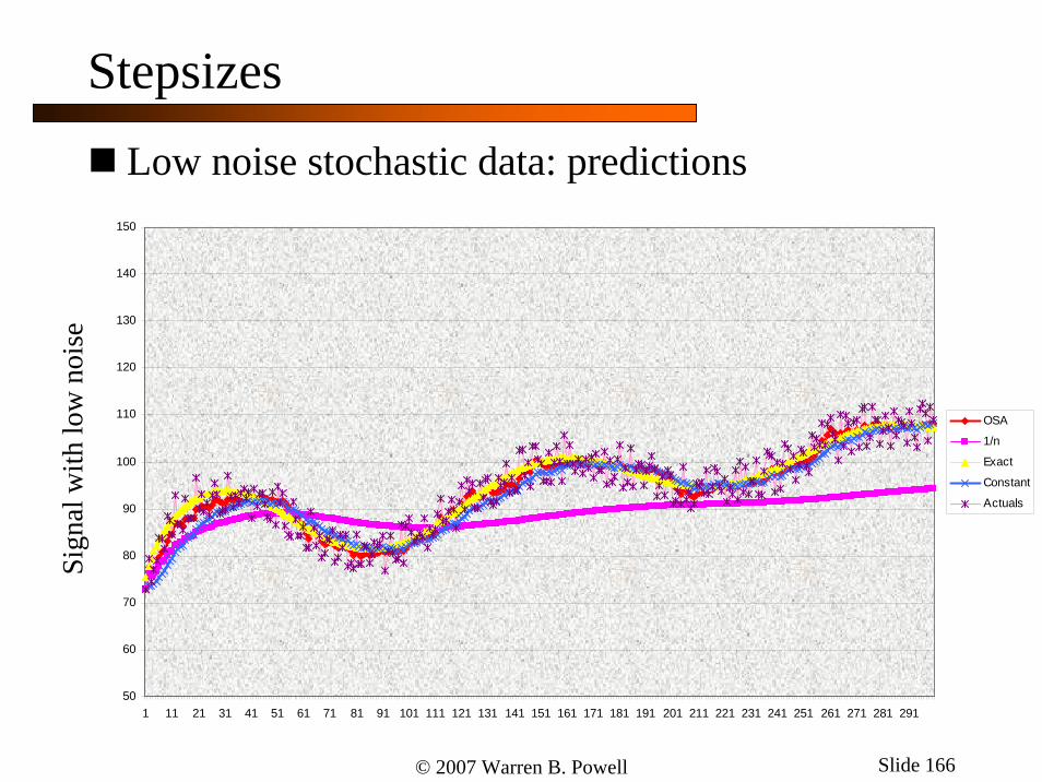
Stepsizes
Low noise stochastic data: predictions
50
60
70
80
90
100
110
120
130
140
150
1 11 21 31 41 51 61 71 81 91 101 111 121 131 141 151 161 171 181 191 201 211 221 231 241 251 261 271 281 291
OSA
1/n
Exact
Constant
Actuals
Sign
al w
ith lo
w n
oise
© 2007 Warren B. Powell Slide 167
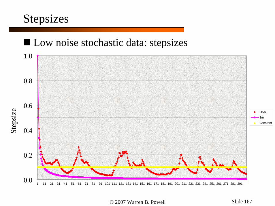
Stepsizes
Low noise stochastic data: stepsizes
0
0.1
0.2
0.3
0.4
0.5
0.6
0.7
0.8
0.9
1
1 11 21 31 41 51 61 71 81 91 101 111 121 131 141 151 161 171 181 191 201 211 221 231 241 251 261 271 281 291
OSA
1/n
Constant
Step
size
1.0
0.8
0.6
0.4
0.2
0.0

© 2007 Warren B. Powell Slide 168
Stepsizes
High noise stochastic data: predictions
50
60
70
80
90
100
110
120
130
140
150
1 10 19 28 37 46 55 64 73 82 91 100 109 118 127 136 145 154 163 172 181 190 199 208 217 226 235 244 253 262 271 280 289 298
OSA1/nExactConstantActuals
Sign
al w
ith h
igh
nois
e
© 2007 Warren B. Powell Slide 169
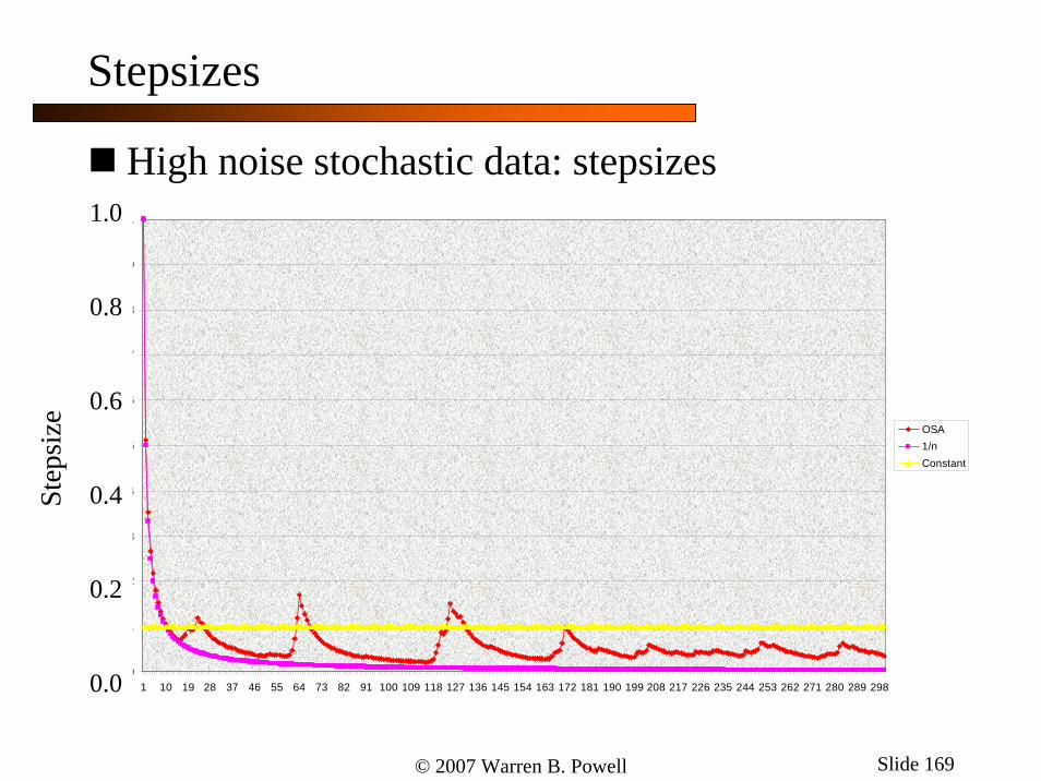
Stepsizes
High noise stochastic data: stepsizes
0
0.1
0.2
0.3
0.4
0.5
0.6
0.7
0.8
0.9
1
1 10 19 28 37 46 55 64 73 82 91 100 109 118 127 136 145 154 163 172 181 190 199 208 217 226 235 244 253 262 271 280 289 298
OSA1/nConstant
Step
size
1.0
0.8
0.6
0.4
0.2
0.0
© 2007 Warren B. Powell Slide 170
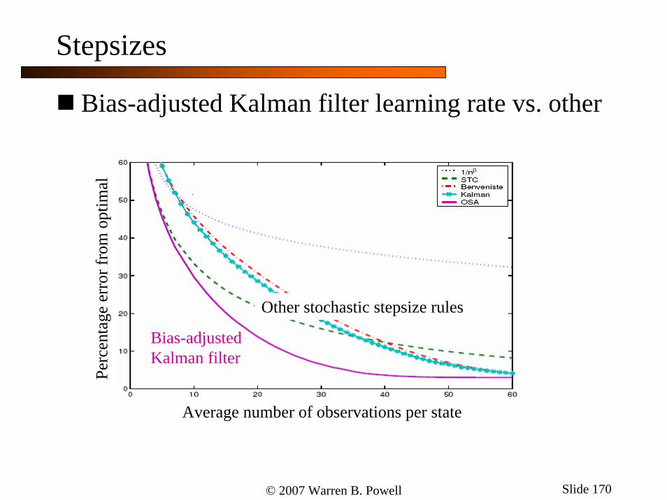
Stepsizes
Bias-adjusted Kalman filter learning rate vs. other stochastic stepsize rules
Perc
enta
ge e
rror
from
opt
imal
Average number of observations per state
Bias-adjustedKalman filter
Other stochastic stepsize rules

© 2007 Warren B. Powell Slide 171
OutlineThe languages of dynamic programmingA resource allocation modelThe post-decision state variableExample: A discrete resource: the nomadic truckerThe states of our systemExample: A continuous resource: blood inventory managementApproximation methods» Lookup tables and aggregation» Basis functions
StepsizesExploration vs. exploitationApplications
© 2007 Warren B. Powell Slide 172
1( , )C a d 2( , )C a d'1( )V a
'2( )V a
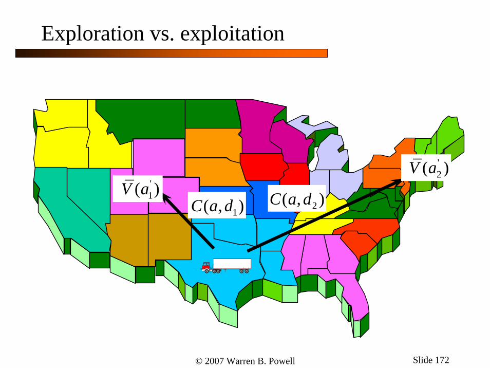
Exploration vs. exploitation

© 2007 Warren B. Powell Slide 173
What decision do we make?
» The one we think is best?
• Exploitation
» Or do we make a decision just to try something and learn more about the result?
• Exploration
Exploration vs. exploitation
© 2007 Warren B. Powell Slide 174
Exploration vs. exploitation with the nomadic trucker
» Pure exploitation
Exploration vs. exploitation
© 2007 Warren B. Powell Slide 175
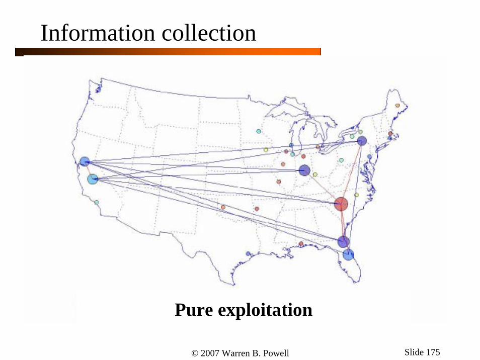
Information collection
Pure exploitation

© 2007 Warren B. Powell Slide 176
Exploration vs. exploitation
The state variable:
( )( )1 1, , n nt t t tS a V σ− −=
“Resource state” Knowledge state

© 2007 Warren B. Powell Slide 177
Resource allocation
1
2
n
aa
a
⎡ ⎤⎢ ⎥⎢ ⎥⎢ ⎥⎢ ⎥⎣ ⎦
M
( )11
110 0 1 1 2 211 12
1213
a a a
aa
w V a w V w V aa
a
⎛ ⎞⎛ ⎞ ⎜ ⎟+ +⎜ ⎟ ⎜ ⎟⎝ ⎠ ⎜ ⎟
⎝ ⎠

© 2007 Warren B. Powell Slide 178
Strategies for overcoming the exploitation trap
» Generalization:• Visit one state, learn something about other states• Exploitation with more general learning
» Gittins exploration
Exploration vs. exploitation
1 1 max ( , ) ( ( , )) ( ) ( ( , ))n n M n Mt d
x C a d V a a d n a a dσ− −= + + Γ
1Std. dev. of ( ( , ))n MV a a d−“Magical index”

© 2007 Warren B. Powell Slide 179
Information collection
Pure exploration

© 2007 Warren B. Powell Slide 180
OutlineThe languages of dynamic programmingA resource allocation modelThe post-decision state variableExample: A discrete resource: the nomadic truckerThe states of our systemExample: A continuous resource: blood inventory managementApproximation methods» Lookup tables and aggregation» Basis functions
StepsizesExploration vs. exploitationApplications

© 2007 Warren B. Powell Slide 181
Schneider National
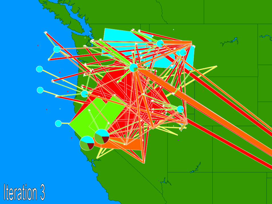
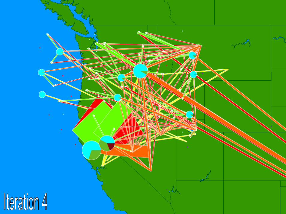
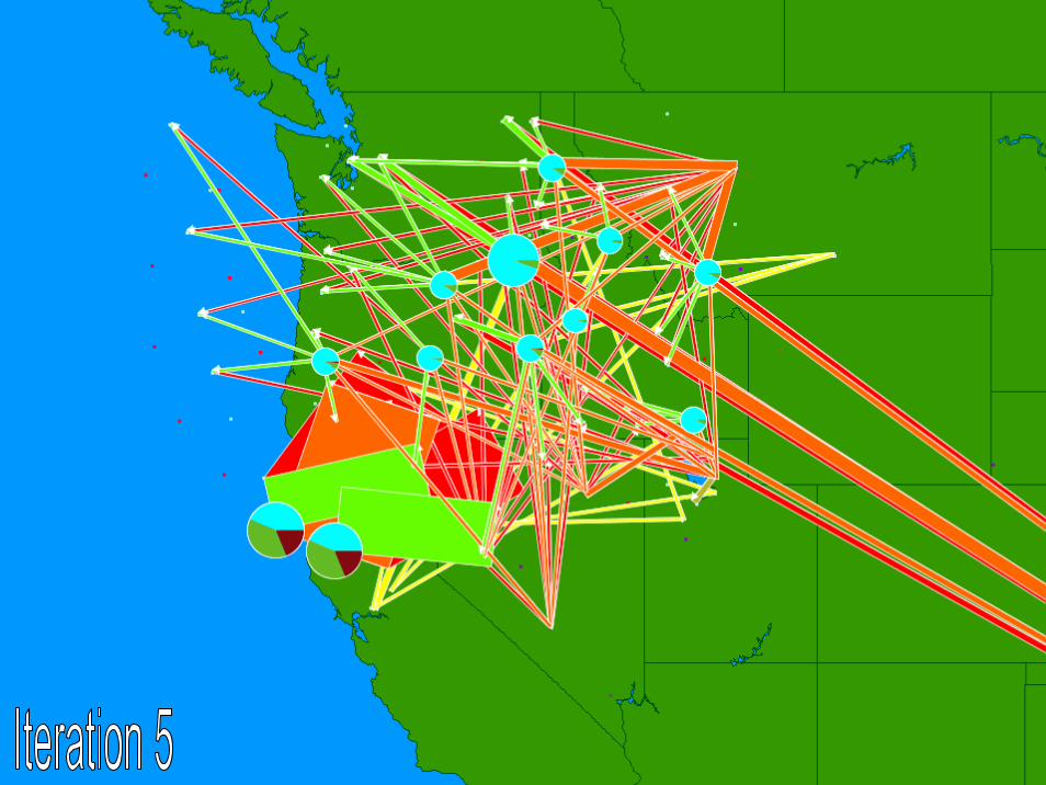
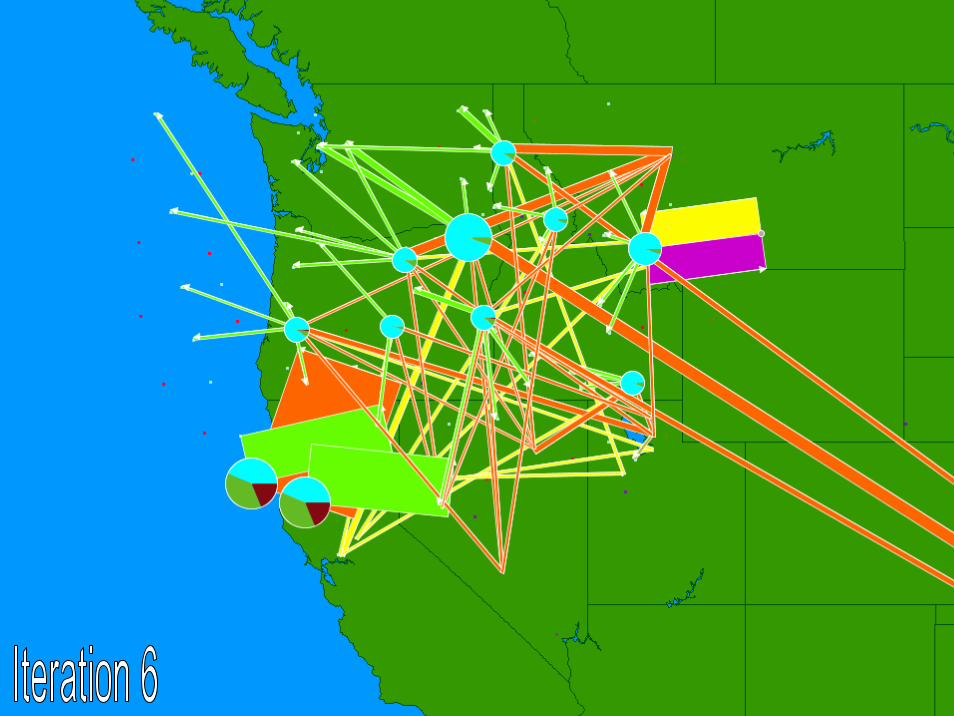
© 2007 Warren B. Powell Slide 182
Schneider National

© 2007 Warren B. Powell Slide 183
© 2007 Warren B. Powell Slide 184
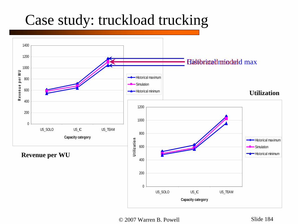
0
200
400
600
800
1000
1200
1400
US_SOLO US_IC US_TEAM
Capacity category
Rev
enue
per
WU
Historical maximum
Simulation
Historical minimum
0
200
400
600
800
1000
1200
US_SOLO US_IC US_TEAM
Capacity category
Util
izat
ion Historical maximum
Simulation
Historical minimumRevenue per WU
Utilization
Case study: truckload trucking
Historical min and maxCalibrated model

© 2007 Warren B. Powell Slide 185
Case study: truckload trucking
Average LOH for Solos
600
650
700
750
800
850
1 3 5 7 9 11 13 15 17 19 21 23 25 27 29 31 33 35 37 39 41 43 45 47 49
Iterations
LOH
(mile
s)
Both Patterns and VFA'sVFA's OnlyPatterns OnlyNo Patterns or VFA'sUBLB
Vanilla simulator
Using approximate dynamic programming
Acceptable region

© 2007 Warren B. Powell Slide 186
Case study: truckload trucking
simulation objective function
1800000
1810000
1820000
1830000
1840000
1850000
1860000
1870000
1880000
1890000
1900000
580 590 600 610 620 630 640 650
# of drivers w ith attribute a
s1
s2
s3
s4
s5
s6
s7
s8
s9
s10
avg
pred

© 2007 Warren B. Powell Slide 187
Case study: truckload trucking
simulation objective function
1800000
1810000
1820000
1830000
1840000
1850000
1860000
1870000
1880000
1890000
1900000
580 590 600 610 620 630 640 650
# of drivers w ith attribute a
s1
s2
s3
s4
s5
s6
s7
s8
s9
s10
avg
pred
av
© 2007 Warren B. Powell Slide 188
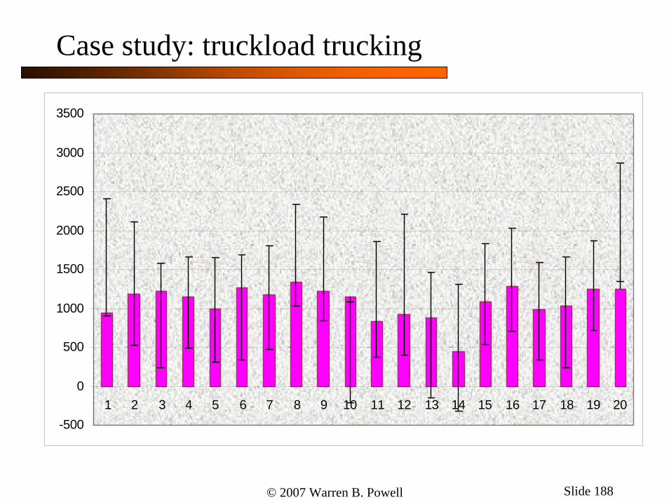
Case study: truckload trucking
-500
0
500
1000
1500
2000
2500
3000
3500
1 2 3 4 5 6 7 8 9 10 11 12 13 14 15 16 17 18 19 20

© 2007 Warren B. Powell Slide 189
Case study: truckload trucking
Iterations
16000000
16500000
17000000
17500000
18000000
18500000
19000000
0 100 200 300 400 500 600
Iteration
Har
d +
soft
$$ p
rofit
Obj
ectiv
e fu
nctio
n
Iterations
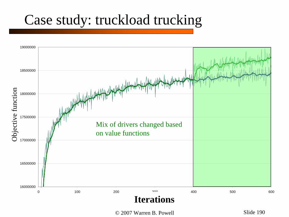
© 2007 Warren B. Powell Slide 190
Case study: truckload trucking
16000000
16500000
17000000
17500000
18000000
18500000
19000000
0 100 200 300 400 500 600
Iteration
Har
d +
soft
$$ p
rofit
Iterations
Obj
ectiv
e fu
nctio
n
Mix of drivers changed based on value functions
Iterations

© 2007 Warren B. Powell Slide 191
Case study: truckload trucking
0
2
4
6
8
10
12
14
16
18
0 100 200 300 400 500 600
Iteration
% D
river
s w
/o T
AH
US
_SO
LO
Iterations
Perc
ent o
f driv
ers n
ot g
ettin
g ho
me
Mix of drivers changed based on value functions

© 2007 Warren B. Powell Slide 192
Case study: truckload trucking

© 2007 Warren B. Powell Slide 193
Case study: truckload trucking
© 2007 Warren B. Powell Slide 194
© 2007 Warren B. Powell Slide 195

© 2007 Warren B. Powell Slide 196

© 2007 Warren B. Powell Slide 197

© 2007 Warren B. Powell Slide 198

© 2007 Warren B. Powell Slide 199
Implementation metricsResults from the real world:
2521
30 32
41
21
37.7
10.6 12
05
1015202530354045
Setouts Swaps Nonpreferredconsists
Underpowered Overpowered
Perc
ent
HistoryModel
© 2007 Warren B. Powell Slide 200
© 2007 Warren B. Powell Slide 201
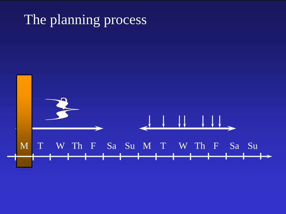
The planning process
M T W Th F Sa Su M T W Th F Sa Su
?

© 2007 Warren B. Powell Slide 202
The flow of information
In practice, there are a number of parallel information processes taking place:
Order is made
Empty transit time to shipper becomes known.
Customer inspects car and accepts or rejects.
Customer loads car (we learn the release time)
Time
Destination of order becomes known

© 2007 Warren B. Powell Slide 203
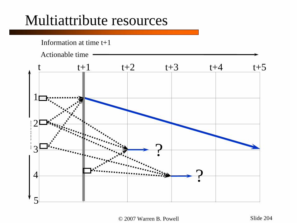
t+1t t+2
4
5
Actionable timeInformation at time t
1
2
3Loc
atio
ns
?
?
t+3 t+4 t+5
?
Multiattribute resources
© 2007 Warren B. Powell Slide 204
t+1t t+2Actionable time
Loca
tions
Information at time t+1
1
2
3
4
5
?
t+3 t+4 t+5
?
Multiattribute resources

© 2007 Warren B. Powell Slide 205
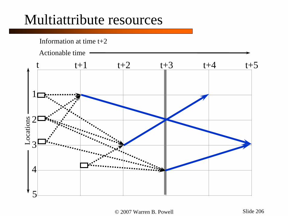
t+1t t+2Actionable timeInformation at time t+2
1
2
3
4
5
Loca
tions
t+3 t+4 t+5
Multiattribute resources
© 2007 Warren B. Powell Slide 206
t+1t t+2Actionable time
t+3 t+4 t+5
Information at time t+2
1
2
3
4
5
Loca
tions
Multiattribute resources
© 2007 Warren B. Powell Slide 207
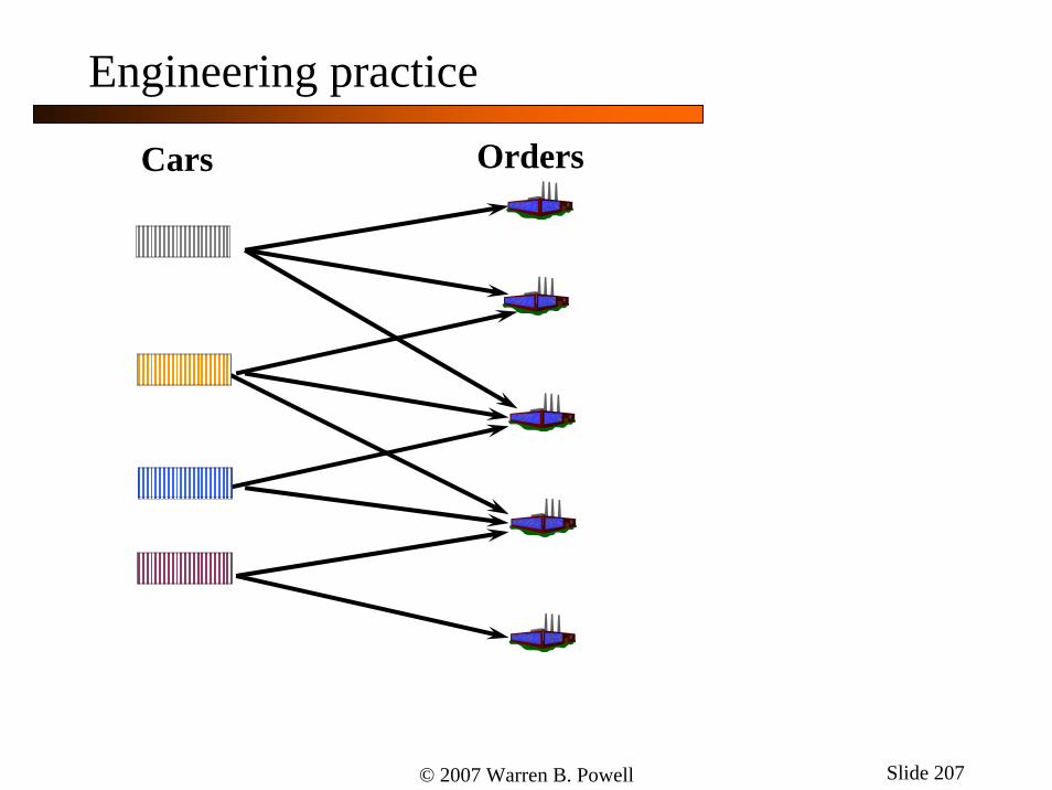
Cars Orders
Engineering practice

© 2007 Warren B. Powell Slide 208
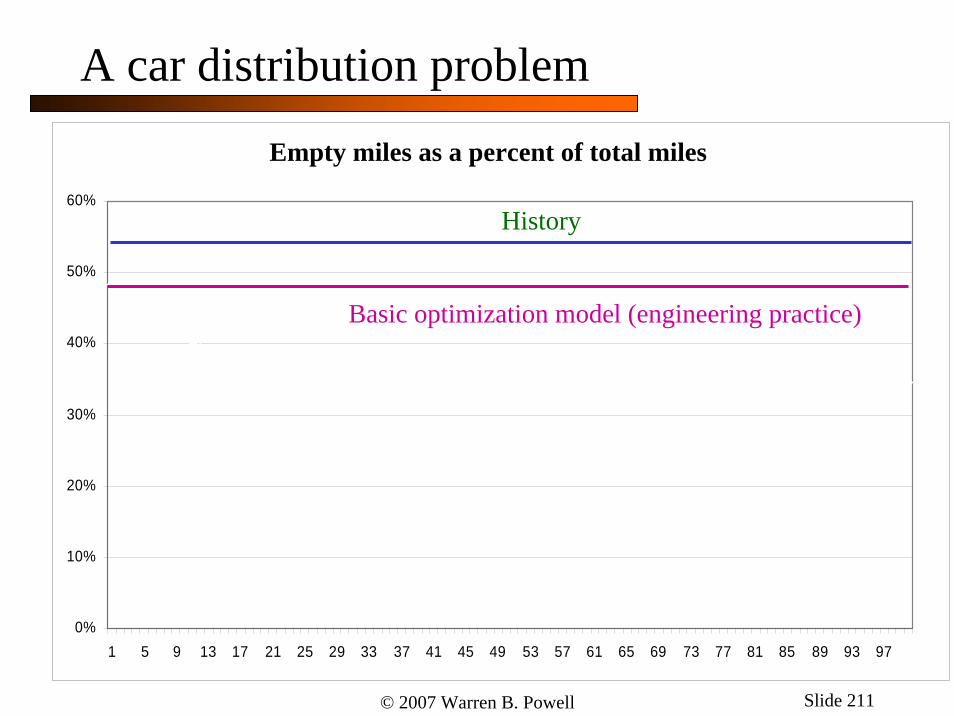
A car distribution problemRatio of Empty Miles to Total Miles Traveled
0%
10%
20%
30%
40%
50%
60%
1 5 9 13 17 21 25 29 33 37 41 45 49 53 57 61 65 69 73 77 81 85 89 93 97
Empty miles as a percent of total miles
History
Basic optimization model (engineering practice)

© 2007 Warren B. Powell Slide 209
Cars Orders
Engineering practice

© 2007 Warren B. Powell Slide 210
Cars Orders
Engineering practice
⎫⎪⎪⎬⎪⎪⎭
Assignments to booked orders.
⎫⎪⎪⎬⎪⎪⎭
Repositioning movements based on forecasts
© 2007 Warren B. Powell Slide 211
A car distribution problemRatio of Empty Miles to Total Miles Traveled
0%
10%
20%
30%
40%
50%
60%
1 5 9 13 17 21 25 29 33 37 41 45 49 53 57 61 65 69 73 77 81 85 89 93 97
Empty miles as a percent of total miles
History
Basic optimization model (engineering practice)

© 2007 Warren B. Powell Slide 212
A car distribution problemRatio of Empty Miles to Total Miles Traveled
0%
10%
20%
30%
40%
50%
60%
1 5 9 13 17 21 25 29 33 37 41 45 49 53 57 61 65 69 73 77 81 85 89 93 97
Empty miles as a percent of total miles
History
Basic optimization model (engineering practice)
“Optimized” with adaptive learning

© 2007 Warren B. Powell Slide 213
© 2007 Warren B. Powell Slide 214
© 2007 Warren B. Powell Slide 215
© 2007 Warren B. Powell Slide 216
© 2007 Warren B. Powell Slide 217

© 2007 Warren B. Powell Slide 218

© 2007 Warren B. Powell Slide 219

© 2007 Warren B. Powell Slide 220
© 2007 Warren B. Powell Slide 221
© 2007 Warren B. Powell Slide 222
© 2007 Warren B. Powell Slide 223
© 2007 Warren B. Powell Slide 224

© 2007 Warren B. Powell Slide 225

© 2007 Warren B. Powell Slide 226

© 2007 Warren B. Powell Slide 227

© 2007 Warren B. Powell Slide 228

© 2007 Warren B. Powell Slide 229

© 2007 Warren B. Powell Slide 230
© 2007 Warren B. Powell Slide 231

© 2007 Warren B. Powell Slide 232
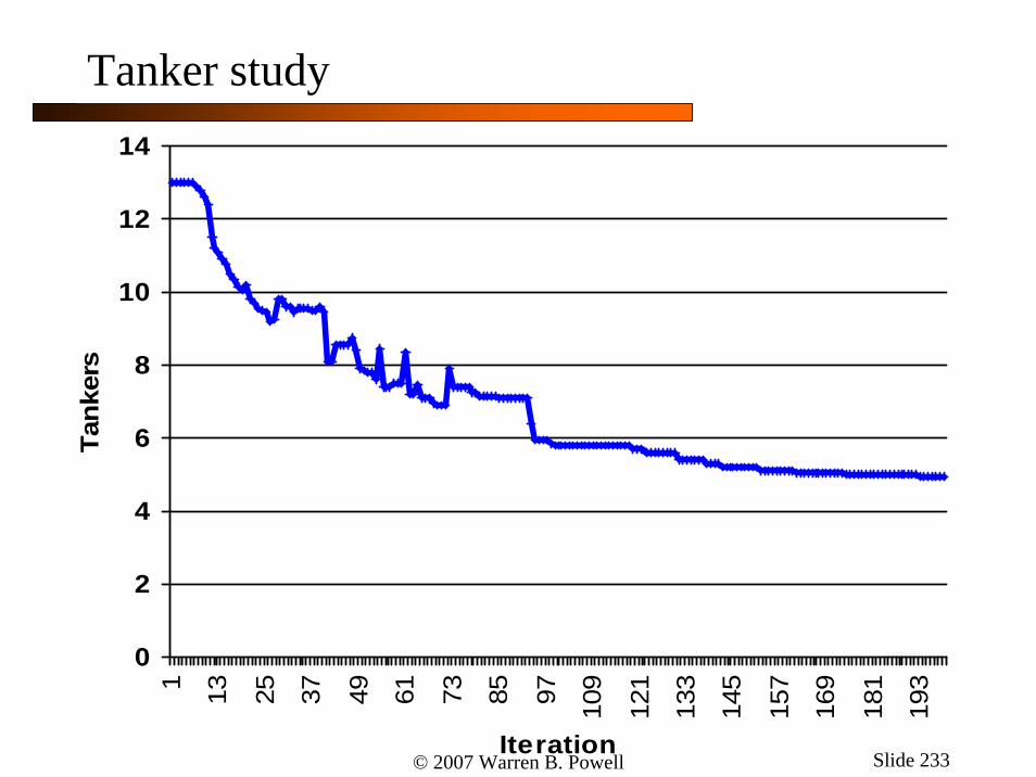
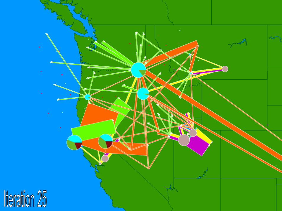
© 2007 Warren B. Powell Slide 233
Average Tankers In Flight per Period
0
2
4
6
8
10
12
141 13 25 37 49 61 73 85 97 109
121
133
145
157
169
181
193
Iteration
Tank
ers
Tanker study

© 2007 Warren B. Powell Slide 234